Local-Scale Groundwater Modeling of Surface–Groundwater Interaction in a Complex Hydrological Setting

Abstract

Sustainable management of hydrogeological systems that supply water and exhibit high hydrologic complexity can be studied through pragmatic numerical modeling supported by field-constrained conceptualization. This study develops a local-scale three-dimensional groundwater flow numerical model using FEFLOW for the Barranca Lebrija settlement in Aguachica town, where the Lebrija River, the Musanda floodplain lake, and groundwater system converge. The numerical model incorporates: (i) the three-dimensional distribution of geological units and lithology; (ii) water level observations from the Musanda floodplain lake; (iii) stage records from the Lebrija River; (iv) boundary conditions and flux estimates inherited from a previous regional groundwater model; and (v) hydraulic heads from two monitoring wells and five community wells. Steady-state and transient conditions were calibrated, and a sensitivity analysis was performed to identify the parameters that most strongly control surface water–groundwater exchange. The simulations reproduce seasonal groundwater level trends and demonstrate the exchange pathways among the river, floodplain lake, and groundwater system. Results indicate dual behavior: during wet periods, flooding of the Musanda floodplain lake driven by high river levels seeps into the underlying aquifer, whereas in dry periods the floodplain lake reverses its role and becomes a principal discharge boundary. This local-scale, boundary-driven approach provides a computationally tractable framework to quantify SW–GW exchange in data-scarce tropical floodplains and supports monitoring design and water-supply management.

1. Introduction

Characterizing river–aquifer systems and surface water–groundwater (SW–GW) exchange remains challenging due to (i) scale mismatches between hydrological forcing and subsurface response, and (ii) uncertainty in hydraulic properties. Riverbed and alluvial heterogeneity control exchange conductance, while river-stage variability can reverse hydraulic gradients and modify source–sink relationships. Moreover, hyporheic–aquifer coupling operates across multiple spatial and temporal scales, and transitions between connected and disconnected states introduce nonlinear and history-dependent responses in variably saturated media [1,2,3,4].

Physically based numerical models have become essential tools for analyzing SW–GW interactions, and their advantages and limitations are well documented in the literature [5,6,7]. These models are generally implemented either as (i) fully coupled surface–subsurface models that co-solve flow equations [8,9,10] or (ii) groundwater models in which surface water dynamics are prescribed as boundary conditions or fluxes [11,12,13,14,15]. While both approaches have advanced the understanding of exchange processes, their practical implementation often faces major constraints. Fully coupled models demand high computational cost and extensive parameterization, whereas boundary-driven groundwater models rely heavily on the availability and quality of hydraulic observations.

A persistent limitation across both strategies is data scarcity. Reliable implementation requires distributed records of river stages, groundwater heads, hydraulic properties, and recharge dynamics. However, datasets are frequently unavailable, particularly in tropical regions and developing countries where groundwater monitoring networks are sparse or non-existent. As a result, many SW–GW studies remain either conceptual or heavily parameterized with poorly constrained inputs.

Additionally, hydrological processes in humid tropical environments introduce further complexity because of greater energy inputs and faster rates of change [16,17]. High annual precipitation, pronounced seasonal variability, intense flood pulses, and strong evapotranspiration create dynamic conditions that can dominate groundwater responses. Large upstream catchments may impose hydraulic signals that propagate into local alluvial aquifers, imprinting seasonal flooding–recession cycles on groundwater levels. Floodplain lakes further complicate connectivity patterns by alternating between periods of surface inundation and partial hydraulic isolation [18,19]. Despite these dynamics, quantitative hydrogeological studies explicitly addressing SW–GW exchange in tropical floodplain systems remain limited.

Importantly, in many tropical settings, groundwater constitutes the primary source of potable water, even in riverine environments. Thus, understanding seasonal exchange reversals and connectivity thresholds is not only of scientific interest but also central to water security [20,21].

In this context, we investigate SW–GW interactions in the Barranca Lebrija area where the Lebrija River and the Musanda floodplain wetland converge within a heterogeneous alluvial aquifer. The regional hydrological system is characterized by (i) high seasonal precipitation (~1000 mm yr⁻¹); (ii) hydrological forcing from a ~9400 km² upstream catchment, which drives recurrent flood pulses; (iii) seasonal wetland inundation with intermittent surface connectivity; and (iv) reliance on groundwater for community water supply despite the riverine setting. However, how these regional controls are transmitted to the local aquifer system remains uncertain, particularly because of SW–GW exchange.

In this context, we established a local groundwater monitoring network comprising monitoring wells, community wells, river and wetland stage measurements, and meteorological observations. These field data were used to constrain a transient, physics-based, variably saturated groundwater model implemented in FEFLOW [22].

Rather than using a fully coupled surface–subsurface solver, we adopted a computationally efficient, boundary-driven modeling strategy in which observed river stages, wetland levels, and inundation extents are imposed as time-varying Dirichlet and Cauchy boundary conditions. This pragmatic framework aligns model complexity with field-measurable variables, enabling parameter constraint under limited-data conditions while capturing the observed seasonal reversals and magnitudes of exchange.

Our aim is to (i) resolve seasonal exchange pathways among the Lebrija River, the Musanda floodplain wetland, and the local aquifer over a complete hydrological year, and (ii) constrain the key hydraulic parameters governing these exchanges in a data-limited tropical setting. By integrating targeted field monitoring with a lean variably saturated modeling framework, this study contributes a transferable approach for SW–GW characterization in humid tropical regions where monitoring networks are scarce.

2. Materials and Methods

2.1. Study Site

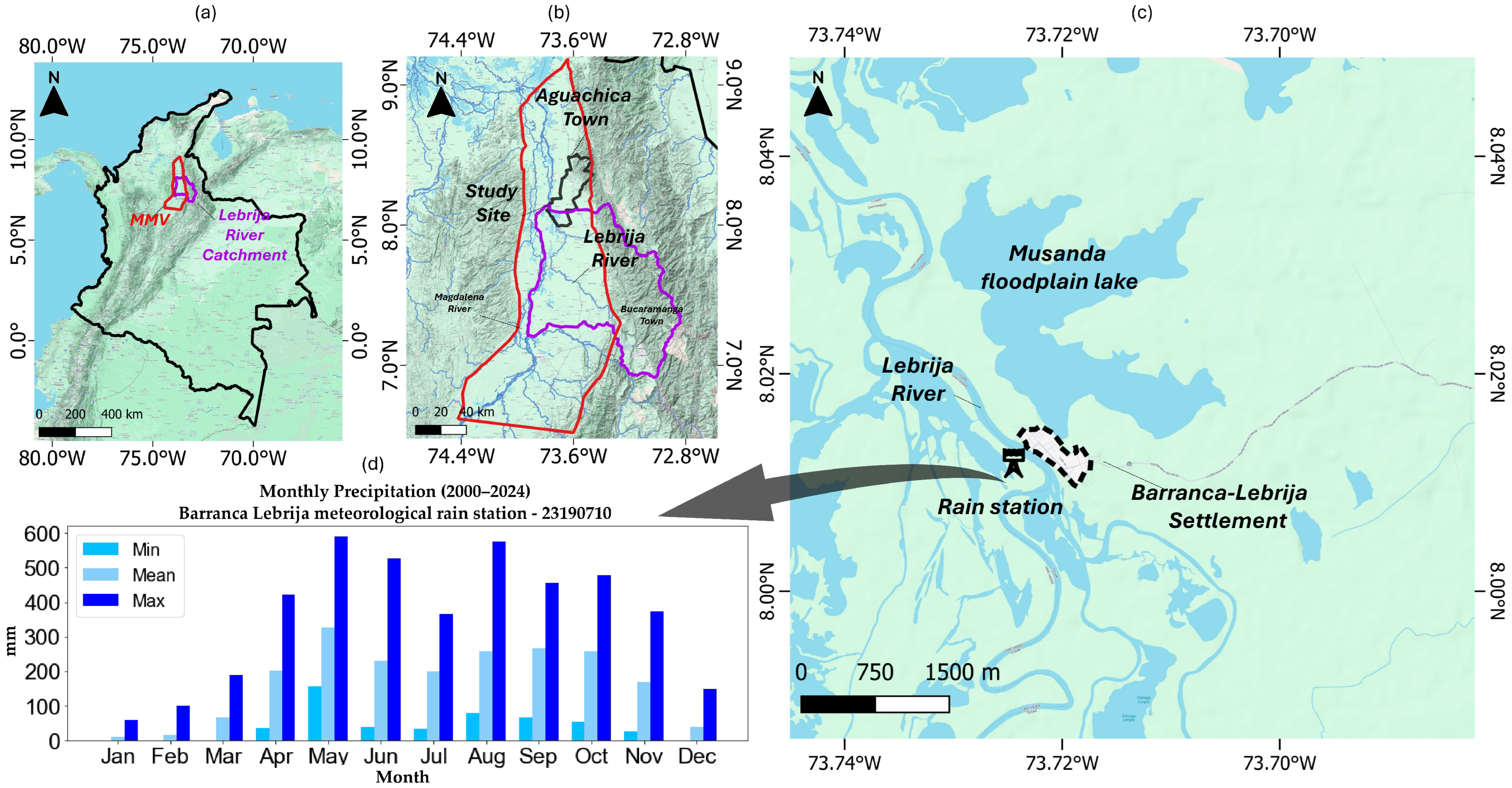
Barranca Lebrija is a small rural settlement of approximately ~2676 inhabitants in the town of Aguachica, Cesar Department, Colombia, within the MMV (Figure 1b). Drinking water is supplied mainly by a single community well that feeds the local aqueduct, with additional use of several shallow household wells scattered around the urban core.

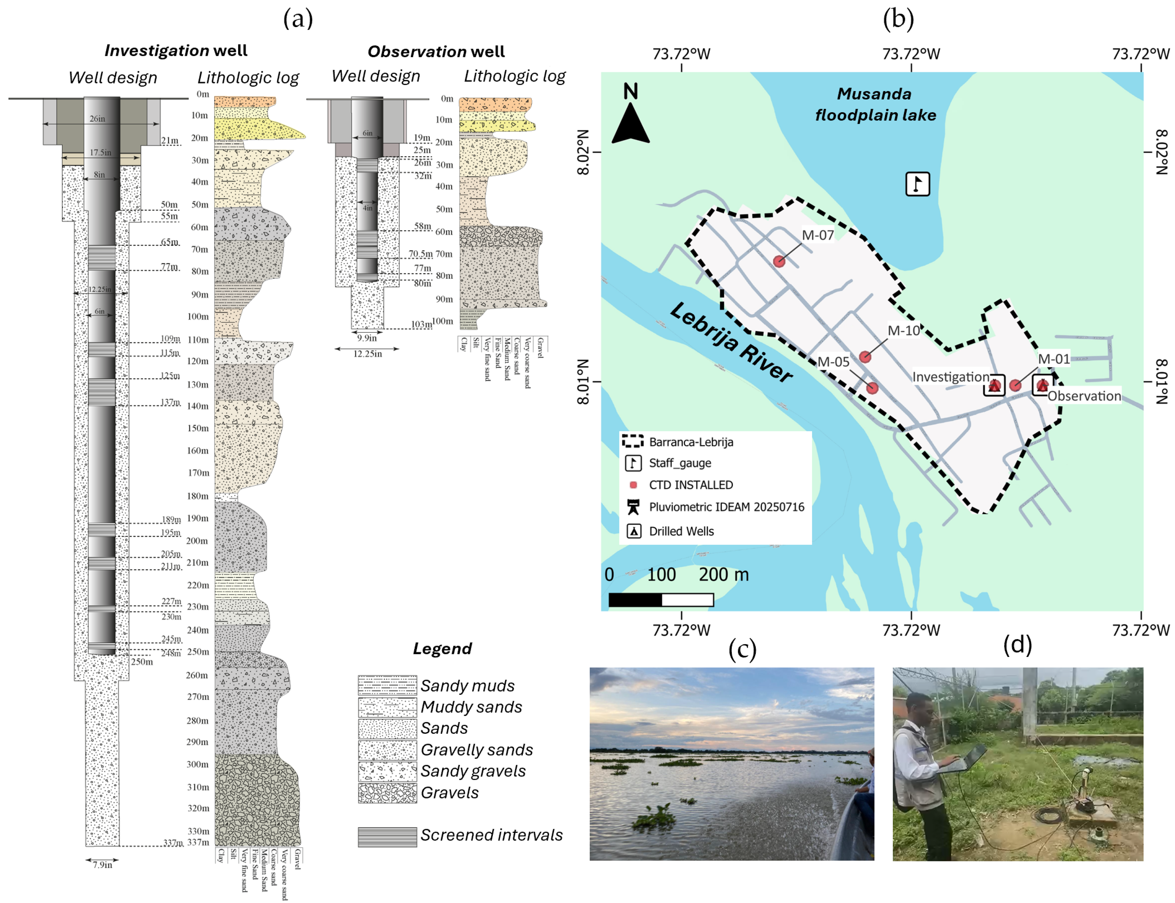
This location has characteristics that make it a suitable natural laboratory for SW–GW interaction research, owing to (i) its highly dynamic surface hydrology, driven by the Lebrija River and the Musanda floodplain lake and (ii) a dedicated monitoring site installed in 2023 that comprises two drilled monitoring wells, a staff gauge installed along the Musanda shoreline, and five community wells equipped with CTD pressure transducers for continuous monitoring of hydraulic head, temperature, and electrical conductivity (Figure 1c).

Topography ranges from ≈19 m a.s.l. in the southwest to ≈50 m a.s.l. in the northeast. Mean monthly precipitation for 2000–2024 is 435 mm yr⁻¹ and displays a bimodal pattern, with pronounced dry seasons from December to January and in minor intensity from June to July [23].

There, the Lebrija River (mean annual flow 150 m³ s⁻¹) constitutes the main fluvial system of the study area and exerts decisive control over SW–GW dynamics. Catchment basin has an approximate area of 9640 km² [24] and has its headwaters in the Eastern Cordillera of the Andes. The river drains into the Magdalena River about 15 km downstream of the study area, in a sector characterized by extensive wetland complexes. Furthermore, it is considered one of the hydrographic basins under the greatest anthropogenic pressure in Colombia, both in terms of water quantity and quality [25]. The hydrological basin supplies drinking water to more than 1,300,000 inhabitants [26], and it faces intense pressure related to water use such as livestock, agriculture, mining, and oil and gas extraction, in addition to numerous wastewater discharges identified in the middle and lower sections of the basin [27].

The hydrological regime is characterized by a bimodal flow pattern primarily governed by the regional precipitation regime [23,26]. In the upper and middle reaches of the Lebrija River, hydrological studies have been conducted by both governmental agencies [24] and academic institutions [26,28]. In addition, community knowledge and practices are shaped by recurrent hydroclimatic cycles that residents recognize and use in daily decision-making [29]. However, the lower hydrological basin lacks hydrometric instrumentation, making flow quantification particularly challenging. This limitation is especially relevant because of the highly dynamic fluvial behavior of the lower river, where the channel becomes poorly defined and disperses into surrounding wetland complexes.

2.2. Regional Hydrogeological Conceptual Model

Regional groundwater understanding in the MMV derives mainly from a regional hydrogeological study [30], complemented by regional analysis of hydrochemistry [31], isotope investigations of SW–GW linkages [32], steady-state numerical groundwater models developed for regional purposes [33,34,35], and local transient numerical modeling [36].

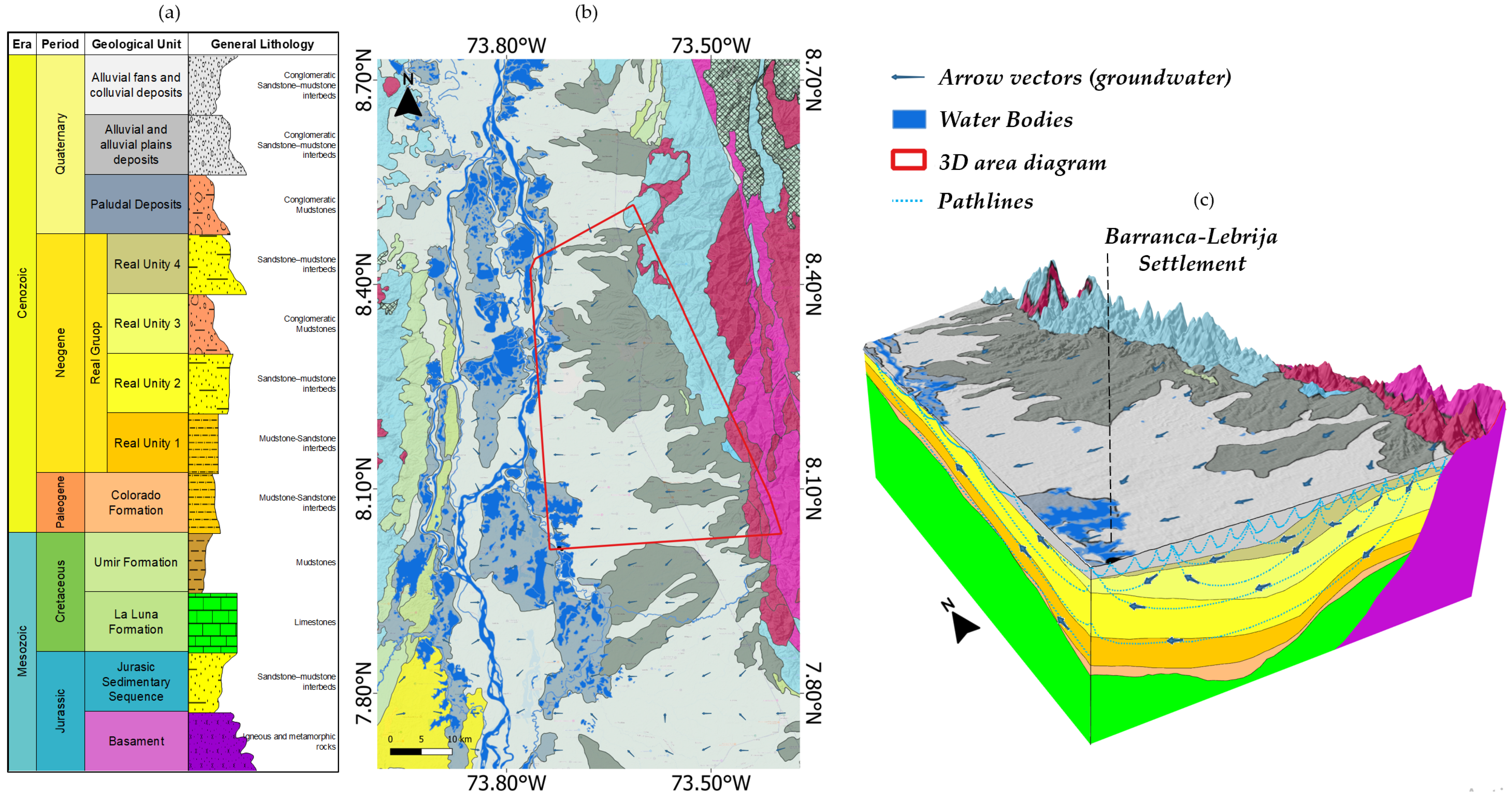
The regional stratigraphy of the MMV comprises Quaternary alluvial and floodplain deposits that overlie the Real Group and the transitional Cenozoic marine sequence and Cretaceous marine strata [37]. Regional hydrogeological syntheses classify the Quaternary deposits and the sand-related units of the Real Group as the principal aquifers of interest (depth < 1000 m) [34]. The Universidad Nacional de Colombia [38] subdivides the Real Group into four successive seismic units, numbered 1 (oldest) to 4 (youngest). Furthermore, lithological logs from the two drilled wells show clast-supported conglomerates with a sandy matrix and minor clay interbeds for Real Group unit 3. Sediment collected from within the Musanda floodplain lake indicates that the lakebed substrate is dominated by silt [39].

A regional compilation of historical hydraulic-conductivity tests in the MMV indicates that Quaternary deposits range from 0.10 to 5 m d⁻¹. For the Real Group units, hydraulic-conductivity values span 0.01–2.10 m d⁻¹, with medians near 0.58 m d⁻¹ [35]. Pumping tests on the monitoring wells corroborate this, yielding sustained discharges of 15–20 L s⁻¹.

Regional piezometric data indicate a regional groundwater flow pattern from the Eastern Cordillera toward the Magdalena Valley, which indicates east-to-west groundwater and discharging into the Lebrija River [34]. Groundwater time series are largely unavailable, representing a critical information gap into the MMV. A graphical summary of the regional hydrogeological conceptual model is presented in Figure 2.

2.3. Field Data

Two monitoring wells were drilled in the study zone. The deepest well (Investigation Well) reaches 250 m and was completed with 48 m of stainless-steel screen. The second well (Observation Well) was drilled to 81 m and includes 21 m of stainless-steel screen; detailed screen placement and construction for both wells are shown in Figure 3a,b.

In addition, six dataloggers (CTD) were installed at community wells and both drilled wells to gather piezometric levels during two periods: from March 2023 to September 2023 and from March 2024 to November 2024.

A staff gauge was installed in the La Musanda floodplain lake and operated from June 2023 to January 2024; despite community surveillance, it was subsequently stolen (Figure 3b,c). Both piezometric and floodplain lake levels were evaluated against rainfall events using precipitation records from the Barranca Lebrija meteorological rain station (ID-23190710).

Thirty-meter-resolution satellite data from the Global Surface Water dataset [41] combined with historical Google Earth imagery were analyzed to evaluate river-swamp dynamics. Recovered water surfaces were used as a time variable boundary condition in the numerical model.

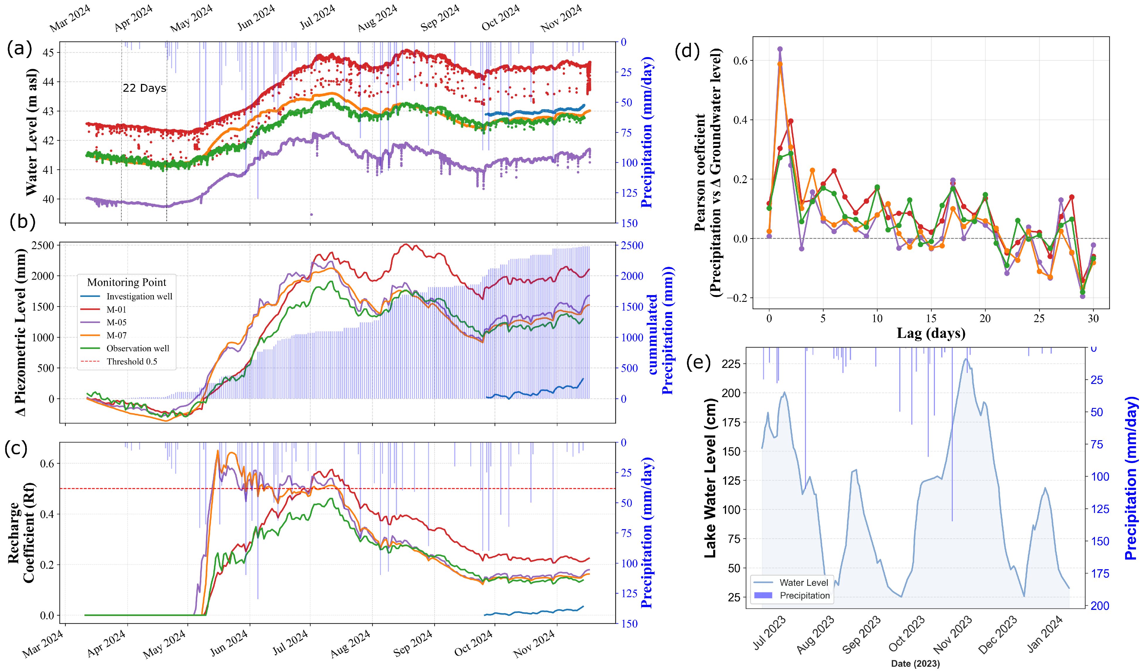
To quantify the temporal response of groundwater levels to precipitation events, a lag correlation analysis was implemented. Daily groundwater level data of each well were paired with daily precipitation records from the Barranca Lebrija hydrometeorological station. Both datasets were aggregated to daily resolution, with groundwater levels represented by daily maximum values and precipitation by daily cumulative totals. The analysis focused on daily groundwater level changes (Δh: Δ piezometric level) rather than absolute levels to emphasize system response dynamics and reduce the influence of long-term trends. Precipitation data were systematically shifted by lag times ranging from 0 to 30 days, and Pearson correlation coefficients were computed between lagged precipitation and daily level changes for each monitoring point. This approach allowed identification of the optimal lag time that maximizes the correlation strength, providing a quantitative measure of the aquifer’s hydraulic response time to recharge events.

2.4. Numerical Model Appoach

Given the study’s requirements for capability, scale, and numerical robustness, FEFLOW Version 8.1 was selected as the modeling platform. FEFLOW is a finite-element model for variably saturated flow governed by the Richards equation. Nonlinearity is solved with Picard/Newton iterations [22]. Surface water is not modeled explicitly; river and floodplain-lake effects are prescribed as time-varying boundary conditions. Transient simulations used a 1-day time step. On a computer unit with an Intel i7 CPU and 64 GB RAM, each transient run requires ~3 h.

2.4.1. Geometry Mesh

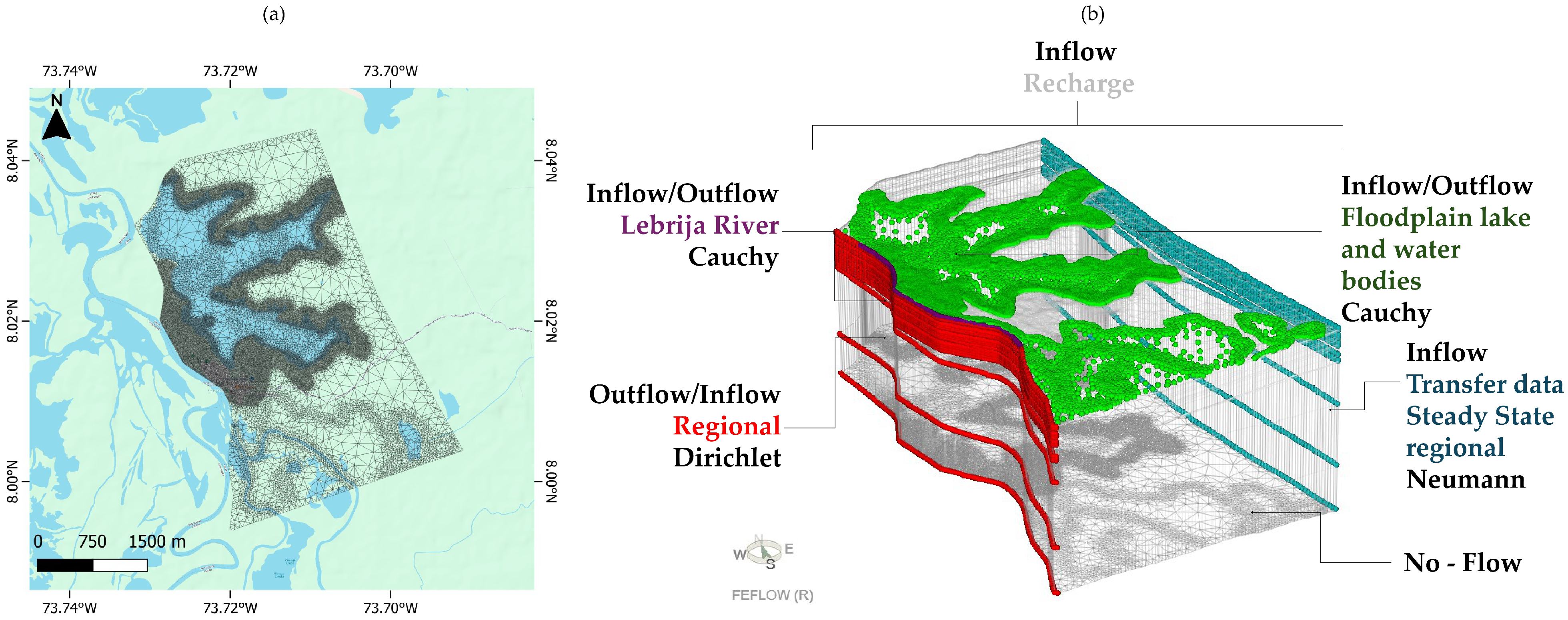
The modeling domain covers 13.3 km² and includes the principal surface water bodies of interest. A 2-D finite-element mesh was generated using the Triangle algorithm [42], with refinement along lake–river margins and around monitoring wells. The 2-D mesh consists of elements with edge lengths shorter than 12 m in data-dense areas, gradually increasing toward the model boundaries.

The 3-D mesh comprises 25 slices and incorporates the seismic-defined geometry of the Real Group units (

Table 1. Layer index correspondence to stratigraphic/topographic surfaces model.

Slice	Surface	Maximum Elevation (m a.s.l.)	Layer Thickness Average (m)
1	Digital Elevation Model	37.0	-
2 to 6	Quaternary Subsurface	35.9	9.4
6 to 14	Quaternary	−5.3	17.2
14	Real 4	−125	31
15	Real 3	−147.2	20
24	Real 2	−830	490
25	Real 1	−1150	320

), with additional vertical refinement at the screened intervals of the monitoring wells. Within the Quaternary deposits, a mesh subdivision at 40 m depth was introduced to improve near-surface resolution. The top boundary follows the ALOS PALSAR DEM with a 12.5 m grid resolution, and the base coincides with the top of the Colorado Formation. The Lebrija riverbed was manually adjusted to 41 m a.s.l. using GPS soundings from January 2025. The final grid contains 27,251 nodes and 53,888 elements.

2.4.2. Boundary Conditions

Boundary conditions represent one of the main sources of uncertainty of the numerical model and are highly dependent on the conceptualization. The locations where boundary conditions were specified are given in Figure 4. Three types of boundary conditions were applied: (i) first type (Dirichlet), boundaries with prescribed hydraulic head, (ii) second type (Neumann) boundaries with specified flux of water, and (iii) third type (Cauchy) that impose a head-dependent flux.

The northern and southern model borders were assigned as no-flow boundaries, assuming that they are approximately parallel to groundwater flow lines. This assumption is based on the potentiometric contours from the regional hydrogeological conceptual model which was developed using more than 3000 groundwater level measurements distributed throughout the basin [34]. These contours indicate that groundwater flow is perpendicular to the equipotential lines in these sectors. This flow pattern is also consistent with regional numerical groundwater models developed for the MMV [33,36].

In addition, regional flow boundary was applied as a Neumann condition and assigned separately to each stratigraphic unit. This condition accounts for the regional lateral continuity of the stratigraphic units represented in the local model, which remain hydraulically connected to the surrounding regional groundwater system. The imposed flux values were taken from the regional numerical groundwater model [34] and correspond to an analytical approximation based on Darcy’s law under steady-state conditions. Darcy velocities along this boundary range from 2.0 × 10⁻⁴ to 5.9 × 10⁻³ m d⁻¹, as listed in

Table 2. Eastern-boundary Darcy velocities derived from the regional numerical hydrogeological model.

Unit	K (m d−1)	Distance (m)	HH-1 (m a.s.l.)	HH-2 (m a.s.l.)	Q (m d−1)
Quaternary	1.0	4400	40	31	0.002
Real U4	0.1	4400	40	31	0.0002
Real U3	3.0	4600	40	31	0.0059
Real U2	1.0	4700	40	31	0.0019
Real U1	1.0	4600	40	30	0.0022

.

A constant-head (Dirichlet) boundary of 41 m a.s.l. was assigned to the entire northeastern face of the model, a value that was derived from GPS-based measurements of the Lebrija River stage that approximates the local riverbed elevation. Conceptually, this boundary represents the hydraulic regulation exerted by the Lebrija River. The Dirichlet condition allows groundwater exchange across this boundary according to the hydraulic gradient, although the river is expected to act mainly as a discharge boundary for the groundwater system.

A Neumann boundary was used to represent recharge in both model scenarios applied across the terrestrial portion of the domain. For the steady-state run, there was a uniform annual flux of 300 mm yr⁻¹ [34]. For the transient simulation, the top-layer Neumann boundary was time-varying: daily rainfall records were multiplied by a recharge factor $R_f$. It was estimated using the recharge (R) estimated by the Water Table Fluctuation method [43,44] and the cumulative precipitation measurements in the analyzed period ($Prec$) as $R_f=R/Prec$.

The change in the storage $∆S$ or the $R$ is estimated as

$$∆S=R=S_y{\displaystyle \frac{∆H}{∆t}}$$

(1)

where $∆H$ is the groundwater level rise recorded since dry season and $S_y$ is the specific yield. $S_y$ represents the fraction of total porosity that releases water by gravity drainage and is commonly considered to approximate the drainable effective porosity, $\eta$ [45]. In the absence of site-specific $\eta$ and $S_y$ measurements, we adopted $S_y\approx \eta$ and assumed a value of 0.26 based on collected information for the regional aquifer as a predominantly sandy to sandy-alluvial formation [30,34,35,38], which is supported by lithological records of monitoring wells, and taken for published values for unconsolidated sandy and sandy-gravel aquifers [46,47,48].

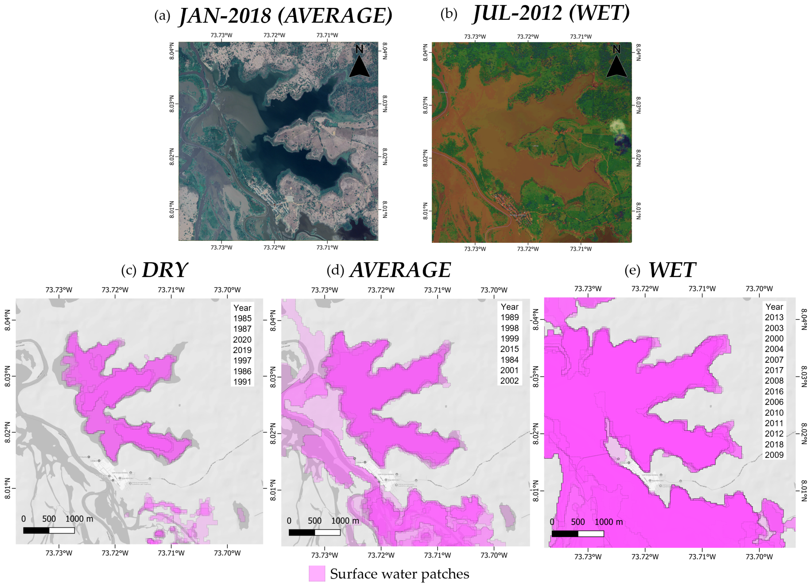
Finally, to represent floodplain lake and water bodies, a Cauchy boundary condition was implemented using a conditional routine developed with the IFM module [49]. This boundary condition is supported by the seasonal hydrological behavior observed in satellite images, which show variable connectivity between the Musanda floodplain lake and the Lebrija River. Figure 5a,b shows the observed water extent during representative dry and wet months, corresponding to January 2018 and July 2012, respectively. Figure 5c–e shows the mean annual floodplain extent for years classified as dry, average, and wet. This classification was based on precipitation anomalies reported by IDEAM [50], complemented by ENSO phases defined by NOAA.

During dry periods, most wetlands tend to become hydraulically disconnected from the river, and some areas may show a predominant hydraulic gradient from the floodplain lake toward the Lebrija River. In contrast, during high river-stage periods, the hydraulic gradient may reverse locally, allowing river water to enter the floodplain lake. Therefore, the river–floodplain lake interaction cannot be represented as a fixed exchange area, but rather as a stage-dependent process controlled by the temporal extent of inundation.

To account for this behavior, the conditional routine compares hydraulic head (H) of waterbody with ground elevation (Z) expressed as Equation (2):

Cauchy activation = 1 if H_waterbody > Z_height; otherwise, 0.

(2)

Thus, a node becomes active whenever H > Z, so the extent of the boundary dynamically reflects the flooded area at a given time step. This head-dependent approach yields a more realistic influence of inundated zones by tying the boundary to the measured or inferred stage in the wetland or river. The higher stage activates a larger set of cells, expanding the Cauchy area in line with observed water-surface extents. For the steady-state simulation, the boundary was implemented using the average-stage scenario (H = 43.1 m a.s.l.).

Conductance term is expressed as Equation (3):

Φ ≈ k_f/d

(3)

The Lakebed thickness (d) is prescribed as the maximum sediment depth reported for MMV wetlands and lakes [39], while riverbed hydraulic conductivity (k_f) is treated as unknown; its sensitivity is discussed below.

2.4.3. Parametrization

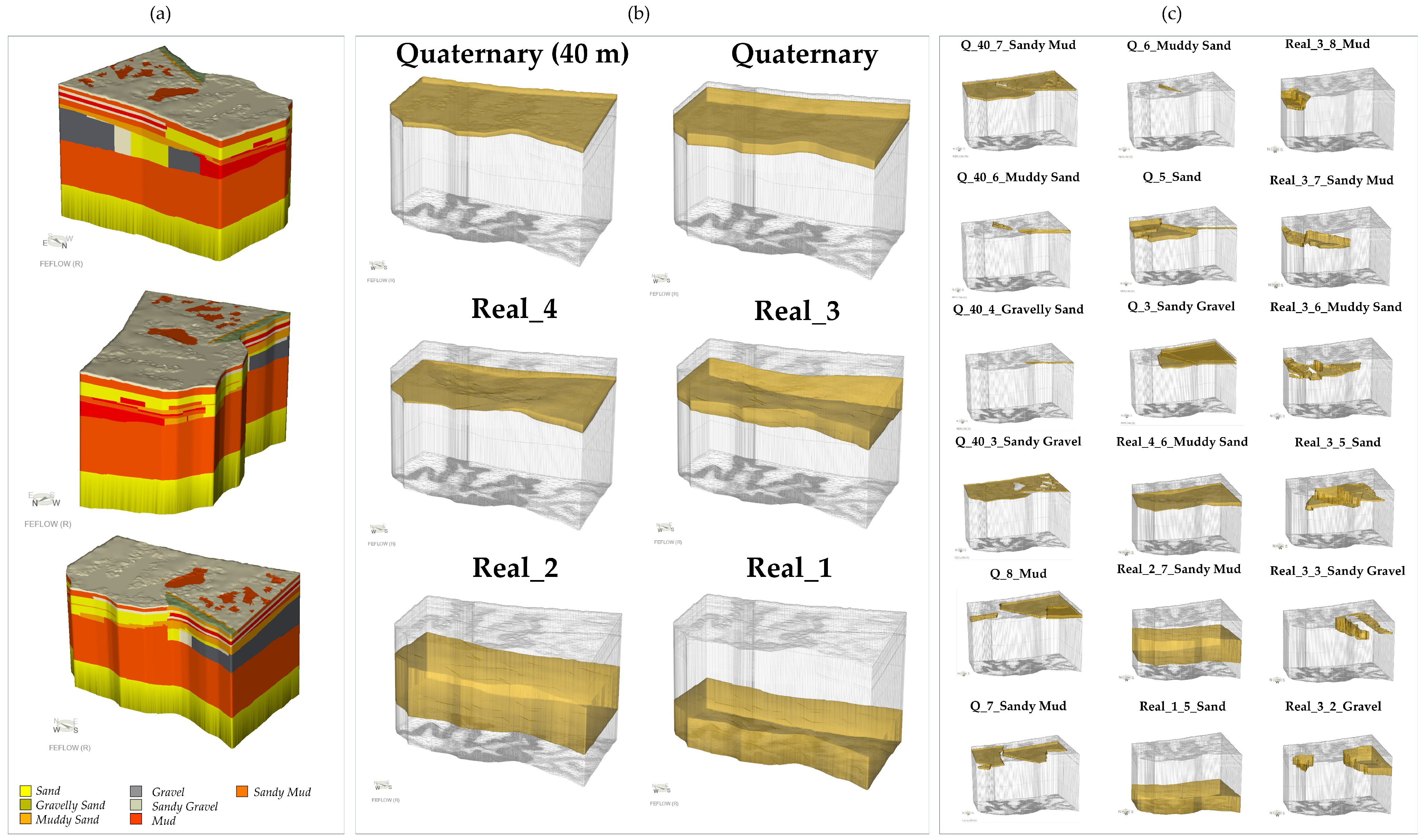
Parameterization allowed hydraulic properties to vary spatially according to the distribution of geological units defined in the conceptual model. Zones were delineated from the 3-D geometric model of seismic units [38].

Lithological data available from 6 well logs were encoded as integer values for each unit and laterally extruded across the 3-D regular mesh with a buffer-expansion algorithm. Propagation was restricted to the horizontal plane preserving the original vertical continuity of each well profile until buffers intersected those of neighboring wells. This procedure discretely interpolated lithology between boreholes and yielded a first-approximation 3-D lithological model.

Subsequently, 18 parameter zones were defined for hydraulic parameter assignment. This zoning scheme was used for the sensitivity analysis and calibration steady and transient model. Figure 6 shows the numerical model units with regional seismic units, and the lithological units identified from local borehole logs.

2.4.4. Sensitivity Analysis and Calibration Workflow

The study area monitoring network comprises seven observation points, with measurements collected during 2023–2024 (

Table A1. Observation points—summary of hydraulic heads and completion characteristics.

Type	FEFLOW ID	Range Dates Datalogger	Average Depth to Water (m)	Elevation (m a.s.l).	Mean HH (m a.s.l.)	Total Depth (m)	Screened Interval Depth (m)
Shallow well	M-01	11 March 2024 to 11 November 2024	6.56	49.59	43.03	20	10
Shallow hand-dug well	M-05	8 June 2023 to 17 November 2024	5.77	48.89	43.12	11	10
Shallow well	M-07	8 June 2023 to 17 November 2024	4.48	47.8	43.32	30	10
Shallow well	M-10	27 May 2023 to 27 September 2023	5.0	46.93	41.93	7.22	6.5
Investigation well	P-R1	26 September 2024 to 14 November 2024	5.5	47.2	41.7	250	77
	P-R2						115
	P-R3						137
	P-R4						195
	P-R5						211
	P-R6						230
	P-R7						248
Observation well	PZ-R1	11 March 2024 to 14 November 2024	6.86	48	41.14	81	32
	PZ-R2						70.5
	PZ-R3						80

). Each well screen interval for the monitoring wells is incorporated as an observation point. Groundwater-head performance was evaluated using Mean Absolute Error (MAE), Root Mean Square (RMS), R² (Pearson Coefficient) and the Kling–Gupta Efficiency (KGE).

Calibration followed a stepwise workflow: (i) a steady-state sensitivity analysis identified the most influential zones and hydraulic-conductivity parameters; (ii) the steady-state model was calibrated to the mean hydraulic head at each observation point (summer conditions); and (iii) the transient model was calibrated under time-varying stresses, reproducing the observed groundwater levels over time (2023–2024).

The sensitivity analysis followed a one-at-a-time (OAT) scheme [51]: either hydraulic conductivity (K), specific storage (S_s) and lakebed hydraulic conductivity (k_f) was perturbed within a single parameter zone while all remaining zones were held at their conceptual values. For the steady-state case, K was varied over 0.001–100 m d⁻¹, yielding 30 simulations per zone evaluating RMS and outputs of balance mass.

3. Results

3.1. Field Data Analysis

Over the hydrological year, groundwater heads declined during dry periods and recovered during wet periods. Two distinct response modes are evident (Figure 7a).

(i).

Early-season storms in March and early April did not trigger an immediate groundwater response. The first significant rainfall event was followed by a delayed rise in piezometric heads of approximately 22 days, and subsequent mid-April rainfall altered the head gradient after ~18 days. This delayed performance is consistent with temporary storage and routing processes within the unsaturated (vadose) zone.

(ii).

During the peak wet season, rainfall events produced near-immediate increases in piezometric levels, with response lags of one day at wells M-05 and M-07 and two days at M-01 and the Observation Well. This rapid response is supported by Pearson correlation coefficients of 0.67, 0.59, 0.40, and 0.29, respectively (Figure 7c), suggesting a clear relationship between precipitation and groundwater level fluctuations.

Lag correlation analysis further reveals spatial variability in hydraulic response across the monitoring network, reflecting heterogeneity in aquifer properties and recharge mechanisms. All monitoring points exhibit peak correlations within 0–10 days, indicating that the primary groundwater response occurs within approximately two weeks following precipitation events. Wells M-05 and M-07, which are closer to the floodplain lake, display higher peak correlations and shorter response times, consistent with stronger hydraulic connectivity and efficient transmission of recharge signals. In contrast, M-01 and the Observation Well show lower peak correlations and slightly longer lags, suggesting the influence of localized heterogeneities, differences in screened intervals, or greater distance from preferential infiltration pathways.

The progressive decline in correlation coefficients at lag times exceeding 15 days indicates that delayed responses contribute minimally to groundwater fluctuations. Overall, the results characterize a hydrogeological system dominated by relatively rapid infiltration and lateral flow processes, although the moderate correlation magnitudes imply that additional controls such as evapotranspiration, pumping, or lateral inflows from adjacent hydrogeological units can modulate piezometric variability.

Analysis of piezometric variations (Figure 7b) reveals clear spatial differences in recharge dynamics among the monitoring wells. Wells M-05 and M-07 exhibit nearly synchronous recovery patterns, characterized by a rapid rise during the first 15 days of the recharge period (steep hydraulic gradients), followed by a sustained increase reaching maximum levels in July. Their proximity to the floodplain lake suggests stronger hydraulic connectivity and a more direct influence of lake-stage fluctuations, resulting in a faster and more pronounced response compared with M-01 and the Observation Well, which are located farther from the lake–aquifer interface and therefore reflect diffuse recharge processes. Groundwater levels declined during the relatively dry intervals in July and September, consistent with reduced recharge and recession of surface water stages, before rising again in response to rainfall events in August and October. During the second wet season (post-October), groundwater levels maintained a slightly positive trend, indicating sustained hydraulic forcing from both local recharge and adjacent surface water bodies.

A comparable initial recovery pattern is observed in M-01 and the Observation Well. However, M-01 exhibited a more pronounced rise, exceeding the recovery observed in the other wells despite similar temporal trends. In contrast, the Observation Well showed the smallest amplitude of variation until August, when changes in piezometric levels became comparable to those recorded in M-05 and M-07.

Comparison between cumulative precipitation and groundwater level rise further highlights system dynamics. Following the first wet season, approximately 1100 mm of accumulated precipitation corresponded to an increase of nearly 2500 mm in groundwater levels. This disproportionate response reinforces the presence of additional recharge sources probably driven by the boundary-controlled response associated with swamps, floodplain lakes, and river stages that rise substantially after rainfall events. However, the lake water level response is not instantaneous (Figure 7e), indicating lagged hydrologic behavior and the influence of regional hydraulic drivers beyond direct local infiltration.

Continuous piezometric monitoring enabled quantification of groundwater level responses to cumulative precipitation through Equation (1). Results indicate convergence of the estimated recharge coefficient to ~0.5 at all monitoring wells by mid-June–July (Figure 7c), at the end of the rainy season, suggesting a consistent recharge fraction across the monitored area during the peak wet season.

Periods of limited cumulative precipitation coincide with declining groundwater levels, reinforcing the strong coupling between rainfall patterns and piezometric response.

3.2. Numerical Model Results

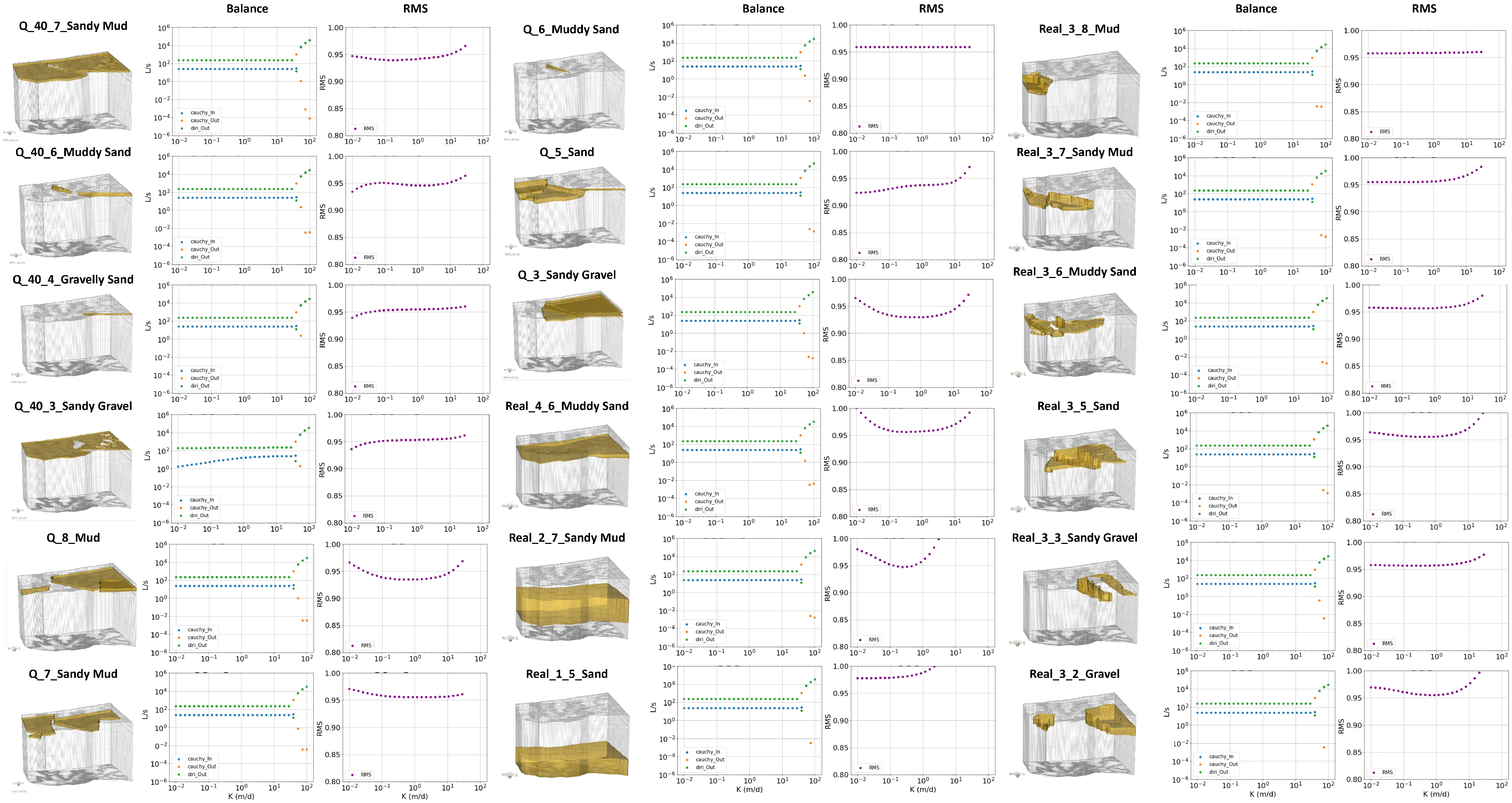
The steady-state sensitivity analysis showed RMS errors between 0.90 and 1.00 for most tested hydraulic-conductivity combinations, whereas larger values were discarded as poorer fits. For K > 50 m d⁻¹, the model exhibits convergence instabilities and RMS ≫ 1.0. The RMS did not decrease below 0.90, suggesting the presence of an irreducible error associated with model structure and data limitation.

Most of the parameter zones showed some degree of sensitivity, with generally better fits at higher K than field-test estimates. This is consistent with a scale mismatch between tests and model resolution. Some parameter zones displayed U-shaped response curves, indicating the existence of an optimal range of hydraulic conductivity values, particularly Q_8_Mud, Q_3_Sandy Gravel, Real_4_6_Muddy Sand, Real_2_7_Sandy Mud. In contrast, Q_6_Muddy Sand and Real_3_8_Mud are insensitive.

Table A2. Interpretive summary of the model sensitivity analysis.

Parameter/Zone	Sensitivity Behavior	Interpretation
High hydraulic-conductivity values, K > 50 m d−1	Numerical instability and RMS ≫ 1.0	Values above this threshold produced convergence problems
Q_8_Mud Q_3_Sandy Gravel Real_4_6_Muddy Sand Real_2_7_Sandy Mud	U-shaped RMS response	Most influential K zones; optimal K range identified
Q_6_Muddy Sand Real_3_8_Mud	Low sensitivity	Limited effect on model fit
Specific storage, Ss	Weak sensitivity	Transient heads weakly constrained by Ss
Lakebed hydraulic conductivity, kf	Low RMS sensitivity but affects exchange fluxes	Head calibration weakly constrains but controls outflow/inflow

presents an interpretive summary of the model sensitivity analysis, whereas Figure A1 presents the steady-state sensitivity results for the hydraulic-conductivity parameter zones.

In the transient simulations, specific storage (Ss) showed weak sensitivity. The shallow units (Quaternary and Real 4) did not show significant changes in Ss. Similarly, deepest units (Real 3, Real 2 and Real 1) responses indicate that Ss is weakly sensitive, and values exceeding 1 × 10⁻⁴ m⁻¹ are unrealistic for a confined aquifer.

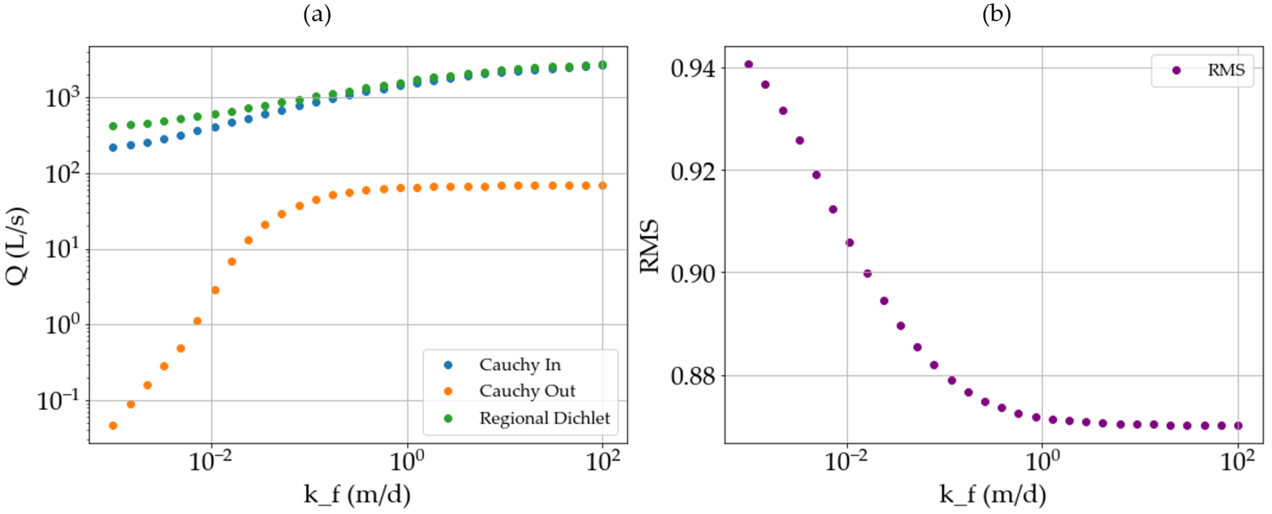
Lakebed hydraulic conductivity (k_f) showed a different type of sensitivity (Figure 8). The RMS error was essentially insensitive across the tested k_f range (between ≈10⁻¹–10⁻² m d⁻¹), indicating that the available hydraulic-head observations do not strongly constrain this parameter. However, k_f directly controls the conductance of the Cauchy boundary and therefore affects the magnitude of simulated surface water–groundwater exchange fluxes. Thus, a low RMS sensitivity indicates that head-based calibration alone is insufficient to constrain exchange processes. Based on the sensitivity analysis, a spatially uniform conductance of Φ = 0.25 d⁻¹ was prescribed, compatible with k_f ≈ 0.5 m d⁻¹ and a lakebed thickness of approximately 2 m, corresponding to the maximum sediment depth reported for MMV wetlands and lakes [39]. Reported muddy-bed hydraulic conductivities of approximately 0.5 m d⁻¹ in comparable settings [1,52] are consistent with this parameterization.

Steady-state calibration yielded RMSE = 1.05 m, MAE = 0.81 m, and a negligible mass-balance residual (−0.0167 L s⁻¹), indicating low error and mass conservation within expected numerical tolerances.

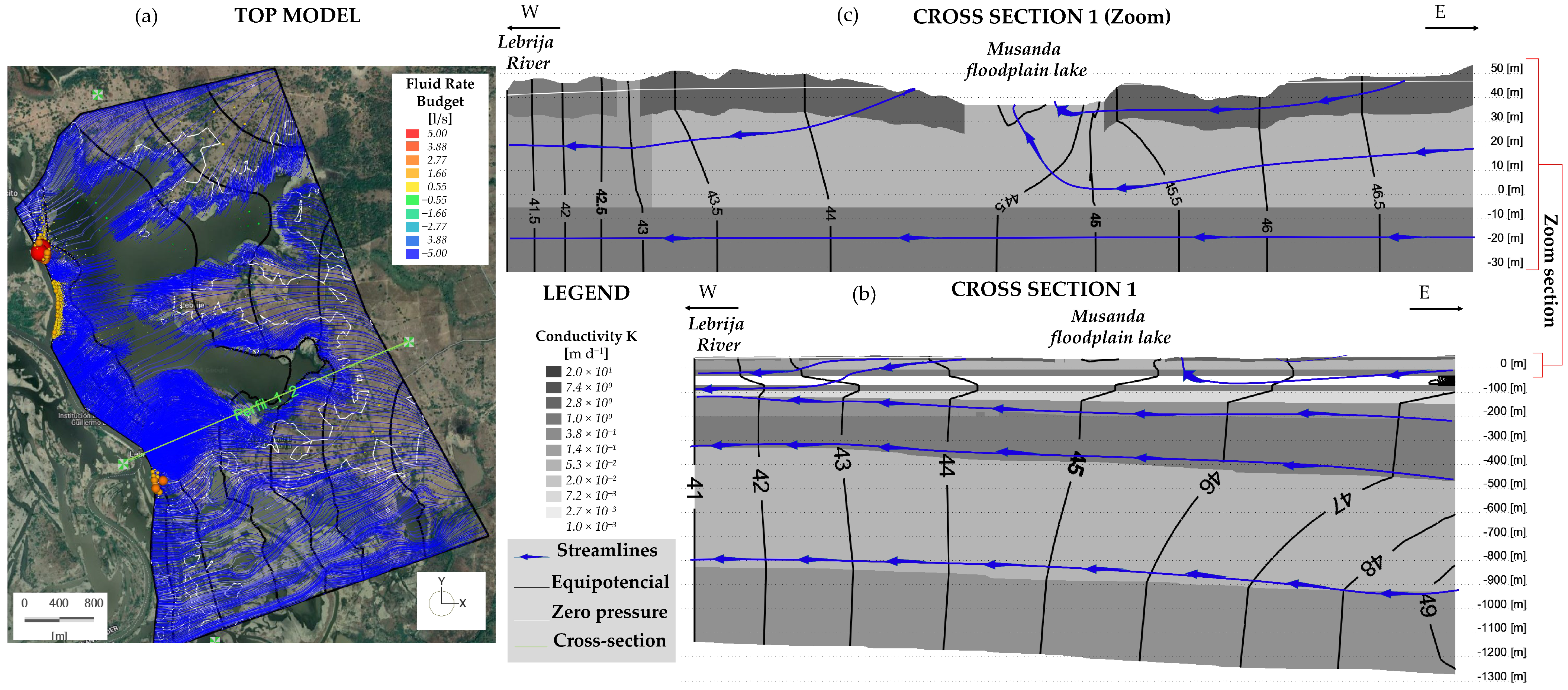
The steady-state results are shown in Figure 9. In the plan-view model results, the simulated streamlines, equipotential contours, and hydraulic-head distribution indicate a predominantly east-to-west groundwater flow system discharging toward the Musanda floodplain lake and the Lebrija River. This behavior is also observed in the representative cross-section across the Musanda floodplain shown in Figure 9b, where the floodplain lake acts as a local discharge zone in shallow depth. However, at the regional scale, the main discharge boundary of the hydrogeological system is represented by the Lebrija River. This flux is also supported by the fluid-rate budget, which shows negative fluxes through the floodplain lake, indicating groundwater discharge, while the shallow system is locally regulated by inflows from the Lebrija River.

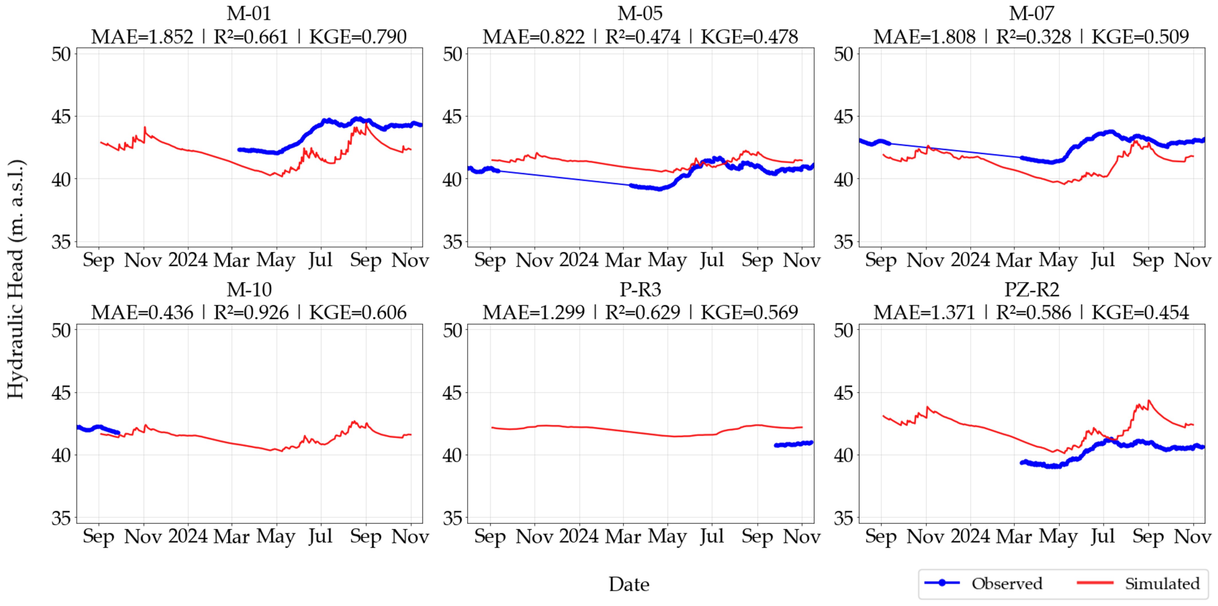
Calibration of the transient model shows that the simulations reproduce the general groundwater-head fluctuations observed at the monitoring points (Figure 10). Model performance was assessed using R², KGE, and MAE. R² values ranged from 0.474 to 0.926, while KGE values ranged from 0.454 to 0.790, indicating variable but generally acceptable performance for a data-limited hydrogeological model [53,54]. Additionally, MAE values remained on the order of a few meters, ranging from 0.436 to 1.852 m.

However, the model showed limitations in reproducing the transient response at some wells, where simulated and observed curves appear temporally shifted, particularly at M-01, M-05 and M-07. This mismatch may be related to the simplified parameterization required to represent a highly heterogeneous hydrogeological system at the model scale. A different behavior is observed at the Observation Well (PZ-R2), where measured heads stabilize from July onward, while the model simulates a rapid rise. This response may indicate local mixing of waters or a hydraulic condition not fully represented by the current parameterization, rather than only a simple head response to recharge. Overall, although the statistics reveal limitations in reproducing local temporal dynamics, the model reasonably captures groundwater-head magnitudes and the main seasonal tendencies, which are consistent with the inherent uncertainty of representing a three-dimensional, heterogeneous subsurface.

The calibrated parameter set (

Table 3. Calibrated hydraulic parameters by parameterization zone. The background colors used for the parameterization units correspond to the stratigraphic chart, whereas the lithology colors are consistent with those shown in Figure 6.

Parametrization Unit	Lithological Unit	K (m/d)	Ss (1/m)
Quaternary Subsurface (40 m depth)	Q_40_7_Sandy Mud	0.1	0.001
	Q_40_6_Muddy Sand	2.5
	Q_40_4_Gravelly Sand	4
	Q_40_3_Sandy Gravel	20
Quaternary	Q_8_Mud	0.001
	Q_7_Sandy Mud	0.01
	Q_6_Muddy Sand	1
	Q_5_Sand	4
	Q_3_Sandy Gravel	0.1
Real_4	Real_4_6_Muddy Sand	1	0.001
Real_3	Real_3_8_Mud	0.001	0.0001
	Real_3_7_Sandy Mud	0.1
	Real_3_6_Muddy Sand	1
	Real_3_5_Sand	4
	Real_3_3_Sandy Gravel	4
	Real_3_2_Gravel	4
Real_2	Real_2_7_Sandy Mud	0.1	0.0001
Real_1	Real_1_5_Sand	1	0.0001

) was represented using internally homogeneous parameter zones. K values span approximately four orders of magnitude, from 1 × 10⁻³ to 2.1 × 10¹ m d⁻¹, with a median value close to 1 m d⁻¹. Mud-rich units are characterized by low K values, ranging from 10⁻³ to 10⁻² m d⁻¹; sandy and silty-sand units show intermediate K values, ranging from 0.05 to 1 m d⁻¹; and sand to gravelly facies show high K values, ranging from 4 to 20 m d⁻¹. These values indicate strong hydraulic heterogeneity within a generally conductive alluvial framework. Specific storage ranges from 1 × 10⁻⁴ to 1 × 10⁻³ m⁻¹, consistent with semi-confined to confined alluvial aquifers [55]. An exception is the Q_3_Sandy Gravel zone, for which the calibrated K value is lower than the range commonly expected for sandy-gravel deposits. This value should not be interpreted as a direct lithological measurement, but rather as a mathematical adjustment resulting from the calibration and sensitivity analysis.

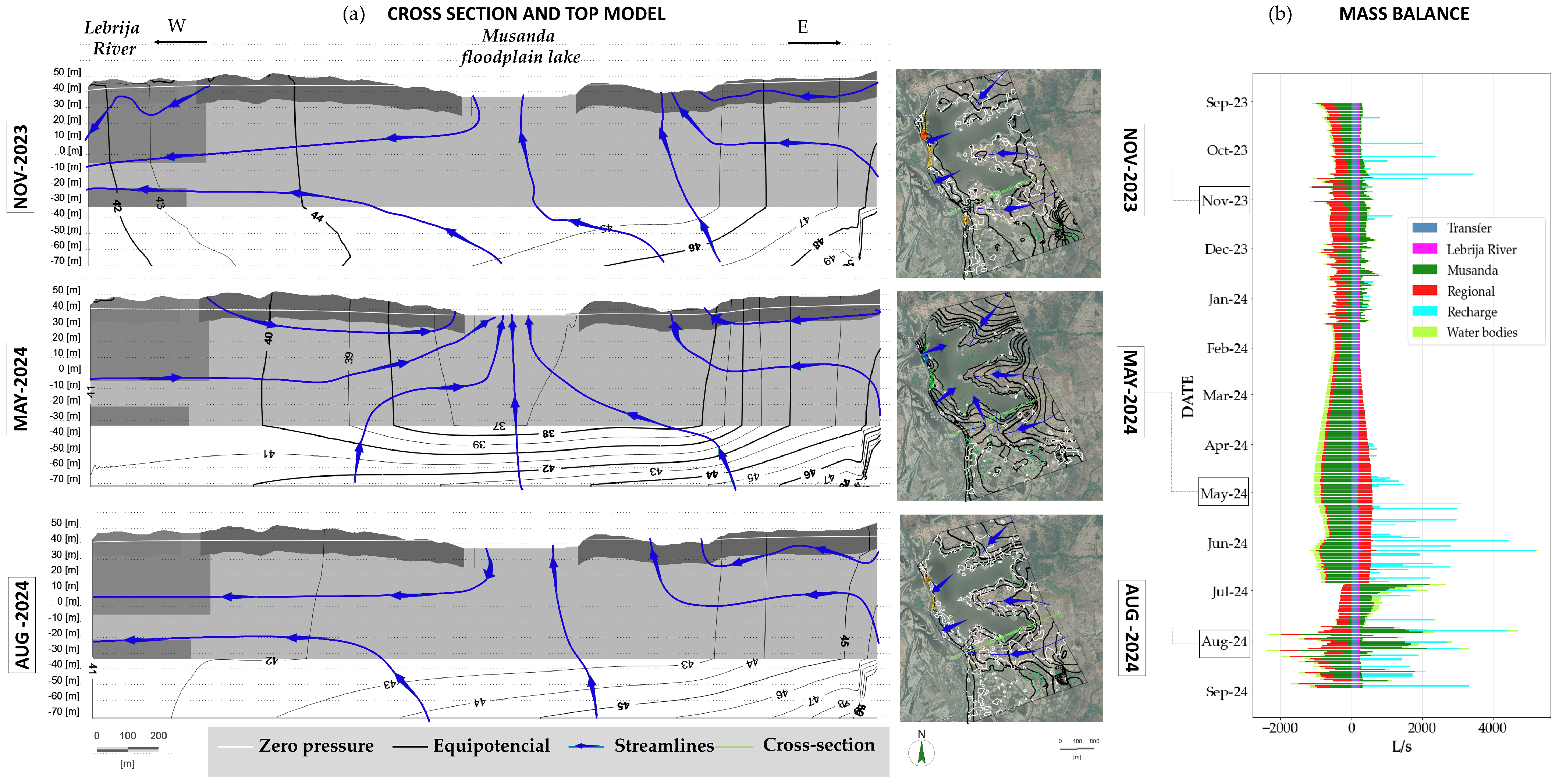
Under transient simulations (Figure 11a), the groundwater system displays a unimodal seasonal signal governed primarily by river-stage variability. Two head-fluctuation regimes emerge from streamlines and equipotential lines: (i) under low river stage and scarce rainfall (February to May 2024), the regional flow field dominates, the Musanda floodplain lake acts as a regional discharge area, and the influence of the deeper Real Group units increases; (ii) during the rainy season (September to January and June to September), fluctuations are locally controlled and exchange among the river, floodplain lake, and aquifer is dominated by flow within the Quaternary deposits.

Mass-balance time series (Figure 11b) reveals a seasonal role reversal at the Musanda floodplain lake (dark green bars). Through dry months (February–May 2024), Musanda inflow is ~0 and recharge are minimal, while Musanda outflow is strongly negative (≈−370 to −600 L s⁻¹), indicating persistent aquifer-to-Musanda drainage and discharge toward the Lebrija River boundary. With the onset of high stage and storm events (June to September), Musanda switches to a source for the aquifer; the modeled reversal occurs on 27 June 2023, driven by recharge–river–groundwater coupling and the build-up of transient storage rather than river stage alone.

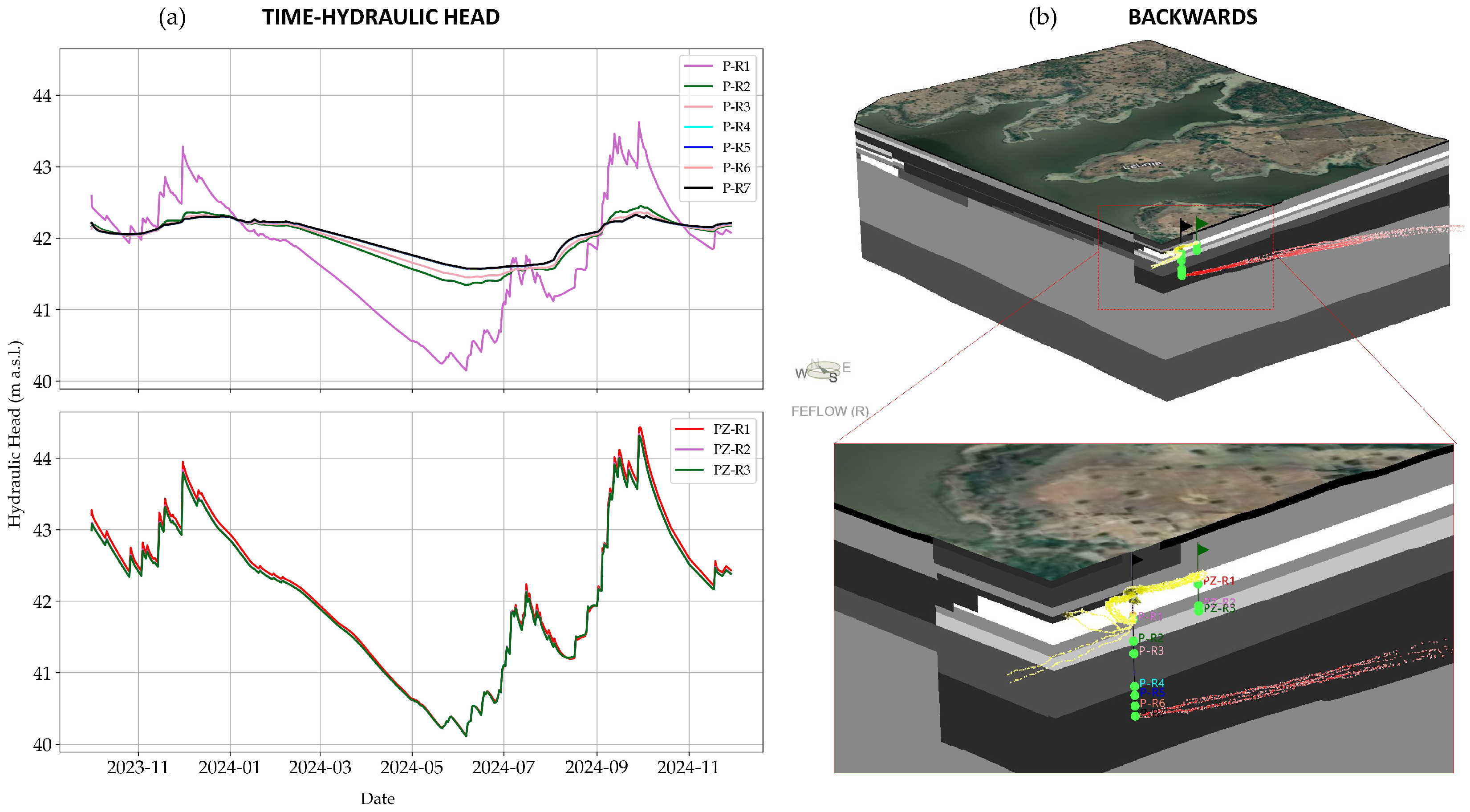
At the well scale, the evaluation of hydraulic heads at the screened intervals (Figure 12) shows that the 20–80 m screens in PZ-R1 exhibit seasonally reversible vertical gradients, whereas the deepest interval in P-R7 (>60 m) indicates a regionally upward-directed gradient. Backward particle tracking supports this interpretation: the shallow PZ-R1 screen receives rapid recharge, as indicated by short travel times; the deeper PZ-R1 screens capture flow from deeper Quaternary strata; and P-R7 shows two provenance domains, one from the shallow Quaternary deposits hydraulically connected to PZ-R1 and another from deeper Real Group units, consistent with regional upwelling.

4. Discussion

Given the well-known scale mismatch in SW–GW studies [1,2,3,6,7,11], we adopted a detailed groundwater model forced with basic field measurements implemented as boundary conditions, including river and floodplain wetland, flood-inundation footprints, and recharge. This scheme transmits the basin-scale hydrological signal without explicitly solving surface-flow hydraulics, while preserving the resolution of locally measurable hydrogeological processes, such as piezometric heads and hydraulic parameters, at a manageable computational cost. However, this pragmatic approach also introduces uncertainty, mainly because the model response depends strongly on the assigned boundary conditions and their conceptual representation. Except for the dynamic Cauchy boundary used to represent flooded areas and imposed recharge, the remaining boundary conditions are static approximations within a naturally transient river–wetland–aquifer system.

Once calibrated and validated, the numerical model reproduces groundwater heads and GW–SW exchange fluxes in the floodplain lake–aquifer system. Its performance, however, is conditioned by limitations: (i) hydraulic heads were recorded as composite responses across multiple screens rather than interval-specific; (ii) wetland stage records are incomplete due to the loss of the staff gauge; (iii) lithological control is sparse and uneven and (iv) the intrinsic hydrological complexity.

Regional hydrogeological numerical models for the MMV report relatively high hydraulic conductivities for Quaternary deposits and the Real Group (≈0.9–20 m d⁻¹) [33,34,35]. In contrast, our local model by explicitly integrating lithologic logs and spatial heterogeneity supports a facies-based conceptualization that is more consistent with field evidence. This representation highlights hydraulic contrasts and low-K lenses that are difficult to capture at regional scale and suggests a multilayered hydrogeologic system, yielding a more realistic, data-supported simulation of flow based on well information and hydraulic tests.

Furthermore, the hydrological setting in Barranca Lebrija (~13 km²) is conditioned by processes operating at the scale of the Lebrija River basin (~4500 km²). In addition, publicly available hydraulic and hydrological data for the lower part of the basin are limited [24]. Therefore, it is known that SW-GW modeling is constrained by data availability [5,56] and that fully coupled models are usually not advantageous when combined with limited data. Representing the full regional hydrologic complexity within a local domain including overbank flooding toward Musanda floodplain lake would require a fully coupled SW–GW model with high computational cost and a risk of obscuring local processes of interest.

Taken together, observations and simulations indicate that, at the study scale, the Musanda floodplain lake acts as a boundary-driven response for the groundwater system, with seasonal reversals of gradients and flow directions: during low-flow periods the aquifer discharges to the wetland, whereas during floods wetland inundation promotes aquifer recharge through the Quaternary deposits, evidencing strong SW–GW interaction in a complex setting. To reduce uncertainty and strengthen the model’s conceptual discretization, continued monitoring (piezometric heads, river and wetland stages, precipitation), incorporation of indirect exploration (geophysics and remote sensing), and improved hydrogeomorphic characterization of the lower Lebrija River basin are recommended.

This study demonstrates that integrating targeted field monitoring with a variably saturated modeling framework provides a transferable strategy for SW–GW characterization in humid tropical regions where monitoring networks are limited or non-existent. Such approaches are particularly relevant in developing-country contexts, where groundwater often sustains potable supply despite complex and dynamic riverine environments.

The present framework therefore provides a defensible basis for local water-security assessment and management, while identifying the additional information required to improve the conceptual understanding of the current river–floodplain lake–aquifer system.

References

1. Fleckenstein, J.H.; Niswonger, R.G.; Fogg, G.E. River-Aquifer Interactions, Geologic Heterogeneity, and Low-Flow Management. Groundwater 2006, 44, 837–852. [Google Scholar] [CrossRef] [PubMed]
2. Irvine, D.J.; Singha, K.; Kurylyk, B.L.; Briggs, M.A.; Sebastian, Y.; Tait, D.R.; Helton, A.M. Groundwater-Surface Water Interactions Research: Past Trends and Future Directions. J. Hydrol. 2024, 644, 132061. [Google Scholar] [CrossRef]
3. Winter, T.C.; Judson, H.; Lenh, F.; Alley, W. Ground Water and Surface Water: A Single Resource; US Geological Survey: Denver, CO, USA, 1999; ISBN 0607893397.
4. Van Genuchten, M.T. A Closed-Form Equation for Predicting the Hydraulic Conductivity of Unsaturated Soils 1. Soil Sci. Soc. Am. J. 1980, 44, 892–898. [Google Scholar] [CrossRef]
5. Barthel, R.; Banzhaf, S. Groundwater and Surface Water Interaction at the Regional-Scale—A Review with Focus on Regional Integrated Models. Water Resour. Manag. 2016, 30, 1–32. [Google Scholar] [CrossRef]
6. Furman, A. Modeling Coupled Surface–Subsurface Flow Processes: A Review. Vadose Zone J. 2008, 7, 741–756. [Google Scholar] [CrossRef]
7. Haque, A.; Salama, A.; Lo, K.; Wu, P. Surface and Groundwater Interactions: A Review of Coupling Strategies in Detailed Domain Models. Hydrology 2021, 8, 35. [Google Scholar] [CrossRef]
8. Dibaj, M.; Javadi, A.A.; Akrami, M.; Ke, K.Y.; Farmani, R.; Tan, Y.C.; Chen, A.S. Coupled Three-Dimensional Modelling of Groundwater-Surface Water Interactions for Management of Seawater Intrusion in Pingtung Plain, Taiwan. J. Hydrol. Reg. Stud. 2021, 36, 100850. [Google Scholar] [CrossRef]
9. Gilbert, J.M.; Maxwell, R.M. Examining Regional Groundwater-Surface Water Dynamics Using an Integrated Hydrologic Model of the San Joaquin River Basin. Hydrol. Earth Syst. Sci. 2017, 21, 923–947. [Google Scholar] [CrossRef]
10. Jones, J.P.; Sudicky, E.A.; McLaren, R.G. Application of a Fully-Integrated Surface-Subsurface Flow Model at the Watershed-Scale: A Case Study. Water Resour. Res. 2008, 44, W03407. [Google Scholar] [CrossRef]
11. Brunner, P.; Simmons, C.T.; Cook, P.G.; Therrien, R. Modeling Surface Water-Groundwater Interaction with MODFLOW: Some Considerations. Ground Water 2010, 48, 174–180. [Google Scholar] [CrossRef] [PubMed]
12. Diaz, M.; Sinicyn, G.; Grodzka-łukaszewska, M. Modelling of Groundwater–Surface Water Interaction Applying the Hyporheic Flux Model. Water 2020, 12, 3303. [Google Scholar] [CrossRef]
13. Haque, A.; Salama, A.; Lo, K.; Wu, P. Development of an Integrated Numerical Flow Model in the Prairie Environment—A Case Study of the Leech Lake Aquifer System, Saskatchewan, Canada. J. Hydrol. Reg. Stud. 2021, 36, 100869. [Google Scholar] [CrossRef]
14. Masterson, J.; Carlson, C.; Walter, D. Hydrogeology and Simulation of Groundwater Flow in the Plymouth-Carver-Kingston-Duxbury Aquifer System, Southeastern Massachusetts; US Government Publishing Office: Washington, DC, USA, 2009; pp. 1–110. [CrossRef]
15. Zeng, J.; Yang, J.; Zha, Y.; Shi, L. Capturing Soil-Water and Groundwater Interactions with an Iterative Feedback Coupling Scheme: New HYDRUS Package for MODFLOW. Hydrol. Earth Syst. Sci. 2019, 23, 637–655. [Google Scholar] [CrossRef]
16. Wohl, E.; Barros, A.; Brunsell, N.; Chappell, N.A.; Coe, M.; Giambelluca, T.; Goldsmith, S.; Harmon, R.; Hendrickx, J.M.H.; Juvik, J.; et al. The Hydrology of the Humid Tropics. Nat. Clim. Change 2012, 2, 655–662. [Google Scholar] [CrossRef]
17. Griesinger, B.; Gladwell, J.S. Hydrology and Water Resources of Tropical Latin America and the Caribbean. In Hydrology and Water Management in the Humid Tropics; Bonell, M., Hufschmidt, M.M., Gladwell, J.S., Eds.; Cambridge University Press: Cambridge, UK, 1993; pp. 84–98. [Google Scholar] [CrossRef]
18. Junk, W.J.; Bayley, P.B.; Sparks, R.E. The Flood Pulse Concept in River-Floodplain Systems. In Proceedings of the International Large River Symposium; Dodge, D.P., Ed.; Canadian Special Publication of Fisheries and Aquatic Sciences; Canadian Department of Fisheries and Oceans: Ottawa, ON, Canada, 1989; Volume 106, pp. 110–127. [Google Scholar]
19. Bonnet, M.P.; Barroux, G.; Martinez, J.M.; Seyler, F.; Moreira-Turcq, P.; Cochonneau, G.; Melack, J.M.; Boaventura, G.; Maurice-Bourgoin, L.; León, J.G.; et al. Floodplain Hydrology in an Amazon Floodplain Lake (Lago Grande de Curuaí). J. Hydrol. 2008, 349, 18–30. [Google Scholar] [CrossRef]
20. World Health Organization; UNICEF. State of the World’s Drinking Water: An Urgent Call to Action to Accelerate Progress on Ensuring Safe Drinking Water for All; World Health Organization: Geneva, Switzerland, 2022; ISBN 9789240060807. [Google Scholar]
21. UNESCO. The United Nations World Water Development Report 2022: Groundwater: Making the Invisible Visible; UNESCO: Paris, France, 2022; ISBN 978-92-3-100507-7. [Google Scholar]
22. DHI-WASI GmbH. Finite Element Subsurface Flow & Transport Simulation System Introductory Tutorial; DHI-WASY GmbH: Hørsholm, Denmark, 2012. [Google Scholar]
23. Cortes, C.; Donado, D.; García, L.D.; Romero, C.; Monrroy, S.; Mancipe, L.F.; Aranda, N.; Niño, T. Balance Hídrico con Información Secundaria del Sector Norte del Valle Medio del Magdalena; Technical Report; Universidad Nacional de Colombia: Bogotá, Colombia, 2025; 239p. [Google Scholar] [CrossRef]
24. CDMB. Plan de Ordenamiento y Manejo de Cuencas Hidrográficas (POMCA) Río Lebrija Medio; Technical Report; Corporación Autónoma Regional para la Defensa de la Meseta de Bucaramanga: Bucaramanga, Colombia, 2019.
25. Rojas, L.P.T.; Díaz-Granados, M. The Construction and Comparison of Regional Drought Severity-Duration-Frequency Curves in Two Colombian River Basins-Study of the Sumapaz and Lebrija Basins. Water 2018, 10, 1453. [Google Scholar] [CrossRef]
26. Gómez, S.; Guzmán, J. Separation of Base Flow in Upper Part of the Lebrija River Basin. Rev. Fac. Ing. Univ. Antioq. 2011, 61, 41–52. [Google Scholar] [CrossRef]
27. García, E.B. Simulación Hidrológica de la Cuenca del Rio Lebrija Mediante El Modelo de Grandes Bacías: Configuración de un Modelo Regional para la Gestión Local de Cuencas. Bachelor’s Thesis, Universidad Pontificia Bolivariana, Bucaramanga, Colombia, 2021. [Google Scholar]
28. Martínez Rodríguez, C. Determinación de Oferta Hídrica de la Cuenca Río Lebrija para El Abastecimiento de Agua para Actividades de Extracción de Hidrocarburos Mediante la Técnica de Fracturamiento Hidráulico en El Municipio de San Martín, Cesar. Bachelor’s Thesis, Universidad del Bosque, Bogotá, Colombia, 2019. [Google Scholar]
29. Murillo, P. Un Mundo Que Se Mueve Como El Río: Historia Regional del Magdalena Medio; Instituto Colombiano de Antropología: Bogotá, Colombia, 1994; ISBN 958-9180-37-X.
30. Servicio Geológico Colombiano. Modelo Hidrogeológico Conceptual Valle Medio del Magdalena, Planchas 108 y 119; Technical Report; Servicio Geológico Colombiano: Bogotá, Colombia, 2019.
31. Malagón, J.P.; Piña, A.; Argüello, S.; Donado, L.D. Hydrogeochemical-Multivariate Analysis of Groundwater in the Aquifer System of the Middle Magdalena Valley, Colombia: Regional-Scale Study. Bol. Soc. Geol. Mex. 2021, 73, A070421. [Google Scholar] [CrossRef]
32. Piña, A.; Donado, L.D.; Silva, L.; Pescador, J. Seasonal and Deep Groundwater-Surface Water Interactions in the Tropical Middle Magdalena River Basin of Colombia. Hydrol. Process. 2022, 36, 14764. [Google Scholar] [CrossRef]
33. Arenas, M.C.; Pescador, J.P.; Garzón, L.D.D.; Saavedra, E.Y.; Obando, P.F.A. Hydrogeological Modeling in Tropical Regions via Feflow. Earth Sci. Res. J. 2020, 24, 283–293. [Google Scholar] [CrossRef]
34. HYDS. Proyecto MEGIA: Producto No. 7, Modelo Hidrodinámico Regional; Technical Report; Universidad Nacional de Colombia: Bogotá, Colombia, 2024. [Google Scholar]
35. Lora-Ariza, B.; Vargas, L.S.; Donado, L.D. Estimation of Hydraulic Conductivity from Well Logs for the Parametrization of Heterogeneous Multilayer Aquifer Systems. Water 2025, 17, 2439. [Google Scholar] [CrossRef]
36. Lora-Ariza, B.; Vargas, L.S.; Pescador, J.; Vaca, M.; Landinez, J.; Piña, A.; Donado, L.D. Numerical Groundwater Flow Modeling in a Tropical Aquifer Under Anthropogenic Pressures: A Case Study in the Middle Magdalena Valley, Colombia. Water 2025, 17, 3579. [Google Scholar] [CrossRef]
37. Sarmiento-Rojas, L.F. Middle Magdalena Basin. Petroleum Geology of Colombia; Technical Report; Agencia Nacional de Hidrocarburos: Bogotá, Colombia, 2011; Volume 11, 193p.
38. Universidad Nacional de Colombia. Proyecto MEGIA: Producto No. 5, Modelo Geológico-Geofísico del Valle Medio del Magdalena (Escala Regional); Technical Report; Universidad Nacional de Colombia: Bogotá, Colombia, 2021. [Google Scholar]
39. Jaramillo, A.; Villamizar, V.; Calvo, J.; Rangel, O.; Parra, N. The Sediments of the Musanda, El Congo, Doña María, El Sordo, Juncal, Baquero, Morales and Castillo Wetlands, Cesar, Colombia; Universidad Nacional de Colombia—Instituto de Ciencias Naturales: Bogotá, Colombia, 2013. [Google Scholar]
40. Gómez, J.; Montes, N.; Nivia, A. Mapa Geológico de Colombia 2015; Servicio Geológico Colombiano: Bogotá, Colombia, 2015. Available online: https://www2.sgc.gov.co/MGC/Paginas/mgc_1M2015.aspx (accessed on 4 January 2025).
41. Pekel, J.F.; Cottam, A.; Gorelick, N.; Belward, A.S. High-Resolution Mapping of Global Surface Water and Its Long-Term Changes. Nature 2016, 540, 418–422. [Google Scholar] [CrossRef] [PubMed]
42. Shewchuk, J.R. Triangle: Engineering a 2D Quality Mesh Generator and Delaunay Triangulator. Appl. Comput. Geom. Towards Geom. Eng. 1996, 1148, 203–222. [Google Scholar] [CrossRef]
43. Meinzer, E. Outline of Ground-Water Hydrology, with Definitions; US Geology Survey Water Supply Paper 494; US Government Publishing Office: Washington, DC, USA, 1923; Volume 8. [CrossRef]
44. Healy, R.W.; Scanlon, B.R. Estimating Groundwater Recharge; Cambridge University Press: Cambridge, UK, 2010; ISBN 9780511780745. [Google Scholar]
45. Fetter, W. Applied Hydrogeology, 4th ed.; Prentice Hall: Upper Saddle River, NJ, USA, 2007; Volume 4, ISBN 978-1-4786-4652-5. [Google Scholar]
46. Johnson, A.I. Specific Yield Compilation of Specific Yields for Various Materials; U.S. Geological Survey Water-Supply Paper; US Government Publishing Office: Washington, DC, USA, 1967. [CrossRef]
47. Woessner, W.; Eileen, P. Hydrogeologic Properties of Earth Materials and Principles of Groundwater Flow; Groundwater Project: Guelph, ON, Canada, 2020; Volume 1. [Google Scholar]
48. Liu, G.; Wilson, B.B.; Bohling, G.C.; Whittemore, D.O.; Butler, J.J. Estimation of Specific Yield for Regional Groundwater Models: Pitfalls, Ramifications, and a Promising Path Forward. Water Resour. Res. 2022, 58, e2021WR030761. [Google Scholar] [CrossRef]
49. DHI IFM (FEFLOW Interface Manager) Documentation. Available online: https://dhi.github.io/ifm/ (accessed on 20 September 2025).
50. IDEAM. Estudio Nacional Del Agua 2022; Instituto de Hidrología, Meteorología y Estudios Ambientales: Bogotá, Colombia, 2023; Volume 1, ISBN 978-958-5489-12-7.
51. ASTM D6511-94; Standard Guide for Conducting a Sensitivity Analysis for a Groundwater Flow Model Application. ASTM International: West Conshohocken, PA, USA, 2008.
52. Di Salvo, C.; Mancini, M.; Moscatelli, M.; Simionato, M.; Cavinato, G.P.; Dimasi, M.; Stigliano, F. From Lithological Modelling to Groundwater Modelling: A Case Study in the Tiber River Alluvial Valley. Geosciences 2021, 11, 507. [Google Scholar] [CrossRef]
53. Anderson, M.P.; Woessner, W.W.; Hunt, R.J. Applied Groundwater Modeling: Simulation of Flow and Advective Transport, 2nd ed.; Academic Press: San Diego, CA, USA, 2015; ISBN 978-0-12-058103-0. [Google Scholar]
54. ASTM D5490; Standard Guide for Comparing Ground-Water Flow Model Simulations to Site-Specific Information. ASTM International: West Conshohocken, PA, USA, 2002.
55. Freeze, A.; Cherry, J. Groundwater; Prentice Hall: Upper Saddle River, NJ, USA, 1979; ISBN 0133653129. [Google Scholar]
56. Brunner, P.; Cook, P.G.; Simmons, C.T. Disconnected Surface Water and Groundwater: From Theory to Practice. Ground Water 2011, 49, 460–467. [Google Scholar] [CrossRef] [PubMed]
Figure 1. (a) The Magdalena Middle Valley (MMV) and Lebrija River catchment location in Colombia, (b) Barranca Lebrija settlement in Aguachica Town, (c) the Lebrija River and the Musanda floodplain lake. (d) Minimum, maximum and mean monthly precipitation in the rain station (ID: 23190710), from 2000 to 2024.
Hydrology 13 00179 g001
Figure 2. (a) Stratigraphic column for the northern MMV, including the informal subdivision of the Real Group into seismic units [38]. (b) Regional geologic map [40] showing the location of the 3-D block diagram and the Barranca Lebrija settlement. (c) Conceptual model illustrating regional groundwater flow as a gravitational system and the location of Barranca Lebrija as a regional outflow.
Hydrology 13 00179 g002
Figure 3. (a) Construction details and screened intervals of the two drilled wells; (b) overview map of monitoring infrastructure (wells, staff gauge in the Musanda wetland, and the meteorological station); (c) staff-gauge site in the Musanda floodplain lake; (d) installation of Keller CTD (conductivity–temperature–depth/pressure) loggers into Investigation and Observation wells.
Hydrology 13 00179 g003
Figure 4. (a) Model area and 2-D finite-element mesh, and (b) spatial distribution of boundary conditions for the local groundwater flow system in the Barranca Lebrija area.
Hydrology 13 00179 g004
Figure 5. (a,b) Google Earth imagery illustrating contrasting hydrologic states: (a) January 2018 (dry year), showing river incursion toward the flood plain lake; (b) July 2021 (wet year), with extensive overbank flooding from the river into the wetland. (ce) Surface water patches identified for years classified according to [41] as (c) dry years (1985, 1986, 1987, 1991, 1997, 2019, and 2020), (d) average years (1984, 1989, 1998, 1999, 2001, 2002, and 2015), and (e) wet years (2000, 2003, 2004, 2006–2013, and 2016–2018), highlighting the wetland’s dependence on river-delivered water.
Hydrology 13 00179 g005
Figure 6. Parameterization of the numerical model. (a) 3-D lithological distribution implemented in the numerical model. (b) Stratigraphic units interpreted from reflection seismic data. (c) Hydraulic parameter zones defined by combining the stratigraphic framework with the estimated lithological distribution. This figure was created using FEFLOW v8.1.
Hydrology 13 00179 g006
Figure 7. (a) Measured groundwater level at M-01, M-05, M-07, Investigation well and Observation well (m a.s.l.), and daily precipitation records at Barranca Lebrija weather gauge (ID 23190710) shown as bars; (b) variation in the piezometric level and cumulated precipitation in bars; (c) estimated recharge coefficient; (d) lag correlation analysis between precipitation and groundwater level changes; (e) relationship between water level recorded at the La Musanda floodplain lake staff gauge and daily rainfall (mm) at the Barranca Lebrija station (ID 23190710).
Hydrology 13 00179 g007
Figure 8. Sensitivity analysis of lake-bed hydraulic conductivity (kf). (a) Fluxes (Q) at the Cauchy inflow, Cauchy outflow, and the model’s eastern Dirichlet boundary that are the main outflow/inflow of model. (b) RMS error.
Hydrology 13 00179 g008
Figure 9. Steady-state model results: (a) Top model showing regional flow from east to west; (b) cross-section 1 across the full depth model domain; (c) zoom of the upper few meters.
Hydrology 13 00179 g009
Figure 10. Simulated and observed hydraulic heads under transient conditions for wells M-01, M-05, M-07, M-10, P-R3 (Investigation Well), and PZ-R2 (Observation Well). M-01 shows a left-shifted simulated response, indicating a slower simulated transition. M-05 and M-07 show right-shifted simulated responses, indicating faster simulated transitions than observed. M-10 and P-R3 reproduce the observed data over their shorter monitoring periods, whereas PZ-R2 does not reproduce the maximum observed peak in September.
Hydrology 13 00179 g010
Figure 11. Transient-state model results. (a) Zoomed cross-section 1 and plan-view results at the model top, slice 1, showing streamlines and equipotential lines for representative months: November, May, and August. In May, the model shows a discharge in flow direction controlled by the floodplain lake. (b) Time-series fluid-rate budget over the simulation period, showing the main boundary-flux components and the July shift in exchange behavior.
Hydrology 13 00179 g011
Figure 12. Well-scale evaluation of vertical hydraulic connectivity. (a) Transient hydraulic heads at screened intervals, showing rapid responses in the shallow intervals of P-R1 and PZ-R1, and more stable behavior in the deeper intervals. (b) Backward particle-tracking results, showing short near-surface flow paths for shallow particles and deeper regional flow paths associated with P-R7.
Hydrology 13 00179 g012