Coupling Modeling Approaches for the Assessment of Runoff Quality in an Urbanizing Catchment

Abstract

The impacts of land use on stormwater runoff quality and Best Management Practices to mitigate these impacts have been investigated since the 1970s, yet challenges remain in providing a modeling approach that concomitantly considers contributions from different land use types. In densely developed urban areas, a buildup/washoff approach is often applied, while in rural areas, some type of erosion modeling is employed, as the processes of detachment, entrainment, and transport are fundamentally different. This study presents a coupled modeling approach within PCSWMM, integrating exponential buildup/washoff for impervious surfaces with the Modified Universal Soil Loss Equation (MUSLE) for pervious areas, including construction sites, to characterize water quality in the large mixed urban–rural Sparrovale catchment in Geelong, Australia. The watershed includes an innovative cascading system of 12 online NbS wetlands along one of the main tributaries, Armstrong Creek, to manage runoff quantity and quality, as well as 16 offline NbS wetlands that are tributary to the online system. A total of 78 samples for Total Suspended Solids (TSS), Total Phosphorus (TP), and Total Nitrogen (TN) were collected from six monitoring sites along Armstrong Creek during wet- and dry-weather events between May and July 2024 for model validation. The data were supplemented with six other catchment stormwater quality datasets collected during earlier studies, which provided an understanding of water quality status for the broader Geelong region. Results showed that average nutrient concentrations across all the sites ranged from 0.44 to 2.66 mg/L for TP and 0.69 to 5.7 mg/L for TN, spanning from within to above the ecological threshold ranges for eutrophication risk (TP: 0.042 to 1 mg/L, TN: 0.3 to 1.5 mg/L). In the study catchment, upstream wetlands reduced pollutant levels; however, downstream wetlands that received runoff from agriculture, residential areas, and, importantly, construction sites, showed a substantial increase in sediment and nutrient concentration. Water quality modeling revealed washoff parameters primarily influenced concentrations from established urban neighborhoods, whereas erosion parameters substantially impacted total pollutant loads for the larger system, demonstrating the importance of integrated modeling for capturing pollutant dynamics in heterogeneous, urbanizing catchments. The study results emphasize the need for spatially targeted management strategies to improve stormwater runoff quality and also show the potential for cascading wetlands to be an important element of the Nature-based Solution (NbS) runoff management system.

1. Introduction

With urban expansion and impervious surfaces replacing natural landscapes, nonpoint source pollution is an environmental concern globally for its impact on the receiving ecosystem [1,2]. The consistently observed ecological deterioration in streams receiving runoff from urban areas led to the introduction of the term “urban stream syndrome” by Walsh et al. [2], which characterizes the common set of ecological symptoms associated with increased urbanization. Progressing from concepts of urban hydrology outlined in the 1960s by Leopold [3], Walsh et al. [2] emphasized that urban streams exhibit flashier hydrographs with more frequent and intense flow compared to non-urban areas, due to the widespread use of traditional stormwater conveyance systems designed for rapid drainage and flood control in urban areas. The flashy flow effect accelerates pollutant transport and simultaneously results in greater peak runoff, total volume, and pollutant loads delivered to downstream environments. Studies have shown that both the concentration and load of pollutants often are higher in urban streams than in non-urban streams [4,5,6]. Pollutant concentrations in streams increase during wet weather events, as accumulated pollutants on the surfaces are dislodged and transported by the kinetic energy of raindrops and the turbulence created by stormwater runoff, a process known as pollutant washoff. Peak concentrations of pollutants such as TSS, however, often occur before peak flow, resulting in a hysteresis effect in the concentration–flow relationship [7]. Climate influences the extent of buildup and washoff, leading to regional differences in urban runoff quality response, as shown in Chaudhary et al. [8], with pollutant concentrations highest in dry climates, followed by continental, temperate, and tropical regions.

The complex, interconnected processes related to pollutant buildup and washoff, and their interaction with surfaces, make urban runoff quality difficult to understand or describe clearly. Regression analysis was among the earliest approaches for modeling urban water quality, with an emphasis on pollutant dynamics at discharge points. Despite advances in data mining techniques such as artificial neural networks (ANNs), the buildup/washoff approach remains widely used since its introduction in the 1970s due to its simplicity and conceptual/physical interpretability [9]. Modern ANN methods require large, high-quality datasets and extensive trial-and-error, limiting their practicality for urban planning under complex dynamic scenarios such as urbanization and climate change [10]. Many studies have applied the buildup/washoff approach to assess water quality at the catchment scale, either on urban residential land use [8,11,12] or mixed land uses [13,14,15]. Pitt et al. [16,17,18] provide a good summary of the historical development in buildup/washoff studies. Generally, the buildup process is represented using some form of a linear, power, exponential, or saturation equation, while washoff is modeled either as an exponential function of runoff or rainfall, using a rating curve, or based on the event mean concentration [14,15,19,20,21,22].

Some studies [8,11] have extended beyond catchment-scale analyses by examining pollutant accumulation and washoff behavior across different climate zones. For temperate regions, accumulated pollutants available for washoff correlate strongly with both average and peak rainfall intensities, producing a relatively consistent and predictable response, as rainfall energy rarely exceeds the 72 mm/h threshold, beyond which raindrop size and kinetic energy plateau, limiting further pollutant mobilization [23]. Bonhomme and Petrucci [24] emphasized that buildup/washoff models assume an “average” surface behavior at the catchment scale and are therefore more accurate when applied to small, specific surfaces (i.e., roads or parking lots). Gaut et al. [15] found that the model tends to lose both physical interpretability and accuracy when applied to larger (>10 ha) and more complex urban catchments. Similarly, although Hossain et al. [25] and Imteaz et al. [26] demonstrated the predictive capability of the buildup/washoff model for a larger catchment (>300 ha) with land uses categorized as pervious and impervious, calibration based on a single rainfall event makes its robustness questionable for long-term water quality prediction. Deletic et al. [27] modified the representation of the washoff process by explicitly modeling overland flow with a kinematic wave approach, coupled with consideration of entrainment through the combined total shear stress of rainfall and runoff, or calculated separately for rainfall and runoff.

Because of the differences in the physical characteristics of source materials (e.g., soil versus dust and dirt accumulation; impact from anthropogenic activities), as well as hydrologic and hydraulic response dynamics (e.g., infiltration, surface roughness, vegetative cover, rain splash, and surface flow stresses), pervious and impervious surfaces will have different contaminant dynamics [28,29]. As such, runoff impact on water quality from pervious areas has been linked to erosion modeling [30,31,32] rather than buildup/washoff. Borrelli et al. [32] in their review of global soil erosion modeling studies found that models based on the Universal Soil Loss Equation (USLE) approach, first introduced in 1965 by the U.S. Department of Agriculture Handbook 282, are the most widely used globally, including in Australia [33,34,35,36,37,38]. USLE-type models describe runoff erosion processes by accounting for factors like rainfall-runoff erosivity (R), soil erodibility (K), slope length and steepness (LS), land cover and management (C), and soil conservation practices (P). Although originally developed and calibrated for agricultural lands, the USLE has been adapted for use on undisturbed areas (i.e., pasture and rangeland) as well as construction sites and in watersheds throughout the world [23,39,40,41,42,43,44,45,46,47]. The USLE (and subsequent versions thereof) allows for a direct representation of detached soil particles and attached pollutant yield from various pervious surfaces, in contrast to models focused on impervious surfaces, where pollutant accumulation and washoff are the dominant mechanisms [46]. While urbanization leads to an overall decrease in erosion at a broad scale as agricultural practices decline [48], concentrated and intense construction activities within urban areas create distinct and severe localized erosion problems [47,49,50].

From our literature review, most studies have applied either the buildup/washoff method or the USLE independently within an urban or urbanizing watershed. While this simplifies the modeling process and is useful in data-limited catchments, it does not capture the variability of surface conditions within a catchment, which can introduce uncertainty in runoff water quality assessments. For example, Hu et al. [47] reported that construction sites can produce sediment concentrations and loads up to an order of magnitude higher than bare, undisturbed land. This suggests that assuming uniform surface behavior may overlook important sources of sediment and pollutant loading, particularly in large, mixed-use catchment areas. Our study addresses this gap by coupling the two modeling approaches to estimate pollutant concentrations and loads from a mixed urban–rural catchment, referred to as the Sparrovale catchment, located in Geelong, VIC, Australia. The specific objectives of this study were to: (1) characterize stormwater quality in the Sparrovale catchment; (2) validate water quality model predictions against measured data to quantify pollutant levels and loads; and (3) assess the variability in pollutant load estimates for the Sparrovale catchment arising from uncertainty in the buildup/washoff and erosion models. This study builds on a previous modeling effort [51] that addressed catchment runoff dynamics and management operations, developed to support Geelong local government in operating an end-of-line nature-based retention feature, Sparrovale Wetland, for management of increasing runoff from urban development. The wetland ultimately serves to protect the downstream Ramsar-listed Lake Connewarre from potential dilution of its brackish water environment. In addition, the catchment features a unique cascading wetland system constructed to manage runoff prior to entering Sparrovale Wetland, though its performance remains unknown. This study places particular emphasis on evaluating this system’s potential to attenuate nutrient (total nitrogen, TN; total phosphorus, TP) and reduce sediment loads (total suspended solids, TSS), providing insight that can inform future design refinements and operational strategies at the final discharge.

2. Materials and Methods

2.1. Study Area

The Sparrovale catchment (Figure 1), located about 11 km southwest of Geelong’s central business district (CBD), includes the Horseshoe Bend and Armstrong Creek areas. Runoff from these areas drains into the 210 ha Sparrovale Wetland, known as a nature-based retention feature, which was converted from farmland to manage runoff and protect the downstream Lake Connewarre Ramsar Site, as noted above [51]. Our study area is 4037 ha in size and is currently undergoing rapid urban development. The proximity of Geelong to Melbourne, which is about 75 km to the east, makes it an important commuter hub, such that suburban development increasingly has expanded into the surrounding area to accommodate the growing population seeking affordable housing and convenient access to the city. As the area continues to develop, Geelong has adopted sustainable urban planning practices, including the preservation of culturally significant indigenous sites and nature-based stormwater management infrastructures that provide co-benefits for community wellbeing and biodiversity support [12,52,53,54].

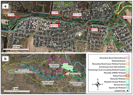
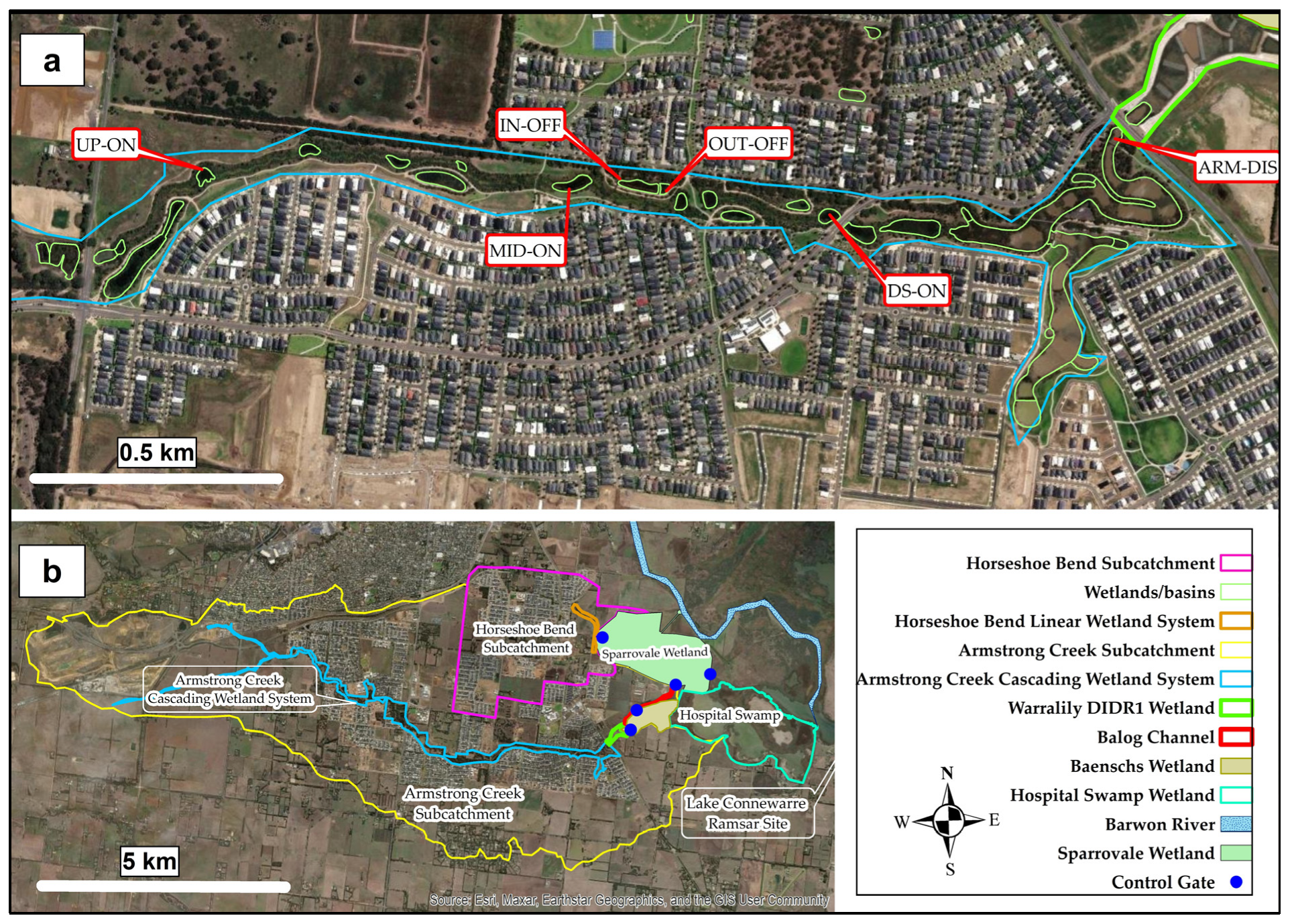
Figure 1. Study area (b) and sampling locations (a) within the Armstrong Creek cascading wetland system.

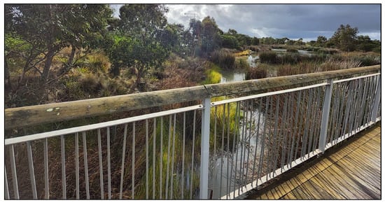
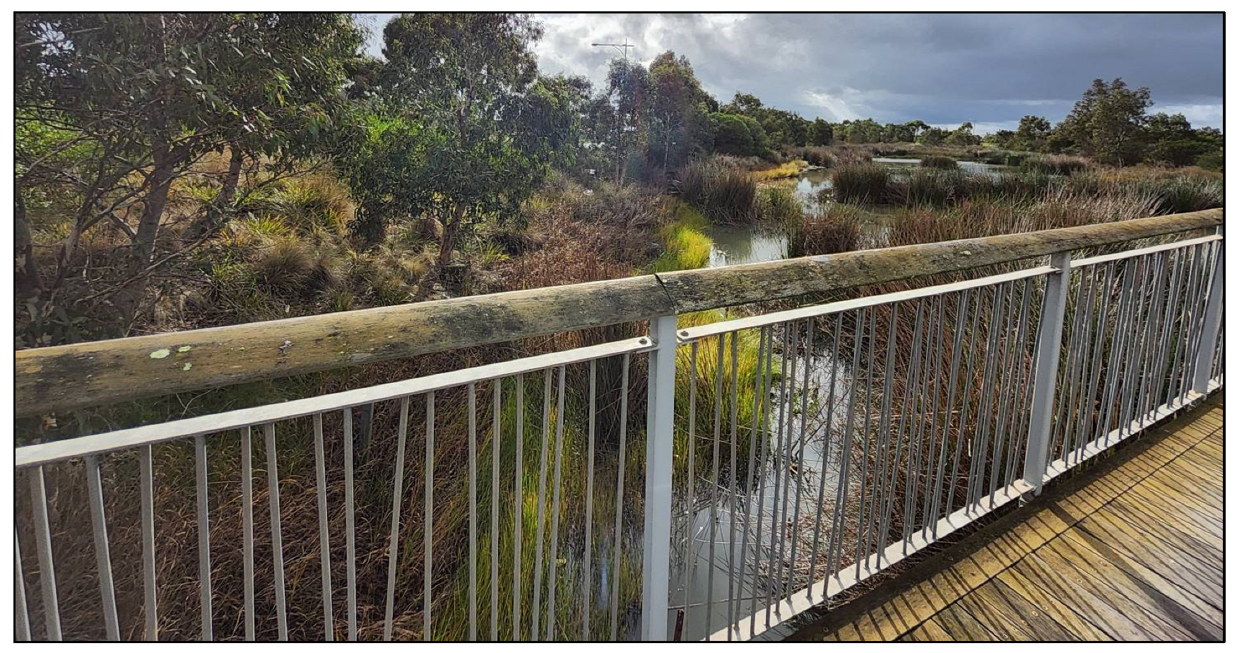
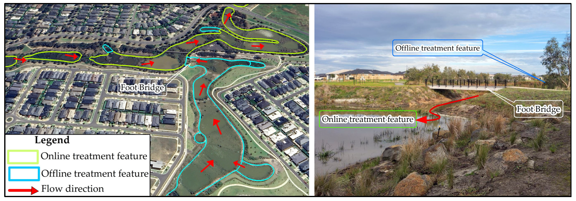
As part of the broader Geelong region, the area is characterized by a temperate marine climate (Cfb) under the Köppen classification system, with average daily minimum and maximum temperatures of 15 °C and 26.4 °C, respectively, and a mean annual rainfall of 516 mm [55] and evapotranspiration of 1076 mm [56]. The Armstrong Creek catchment (Figure 1b) features a cascading wetland system (Figure 1a) consisting of a 9 km-long open drainage channel that contains a series of 12 online detention ponds and linear wetlands (Figure 1a and Figure 2). In this online configuration, stormwater flows sequentially through the ponds or wetlands that are integrated within the main creek channel as part of the continuous drainage pathway. The system is designed to provide treatment and conveyance of runoff from a total catchment area of 3094 ha, primarily residential, open space, and agricultural land uses. Before release into this online system, runoff from the catchment initially is conveyed through offline treatment systems (sedimentation or/and bioretention basins and wetlands) which are positioned adjacent to the online drainage channel (Figure 3) in Armstrong Creek. These basins are designed as pretreatment stormwater features to temporarily hold runoff for a three-day retention period, allowing sediments to settle and improving water quality before the flow is released to the online cascading system. The offline configuration includes 15 sedimentation and one bioretention basins with surface areas ranging from 753 m² to 27,800 m² and estimated depths varying from 1 m to 3.8 m. Runoff from Armstrong Creek subsequently flows into the downstream diversion wetland system, where it is directed either into the Sparrovale Wetland or discharged to the wetland complex immediately upstream of Lake Connewarre. Runoff from the Horseshoe Bend catchment (Figure 1b) is managed in a simpler manner compared to Armstrong Creek, as the area is much smaller (943 ha). Runoff is discharged through a pipe system into a sedimentation basin, which subsequently discharges to the linear wetland upstream (Figure 1b) of Sparrovale Wetland. Greater detail on the stormwater runoff management systems, including the hydraulic structures of the two catchments, can be found in Teang et al. [51].

Figure 2. An example of online detention ponds and wetlands connected within the larger Armstrong Creek cascading wetland system.

Figure 3. An example of offline and online treatment features as a connected system for residential areas in the Armstrong Creek catchment.

2.2. Runoff Water Quality Data

2.2.1. Sampling and Laboratory Methods

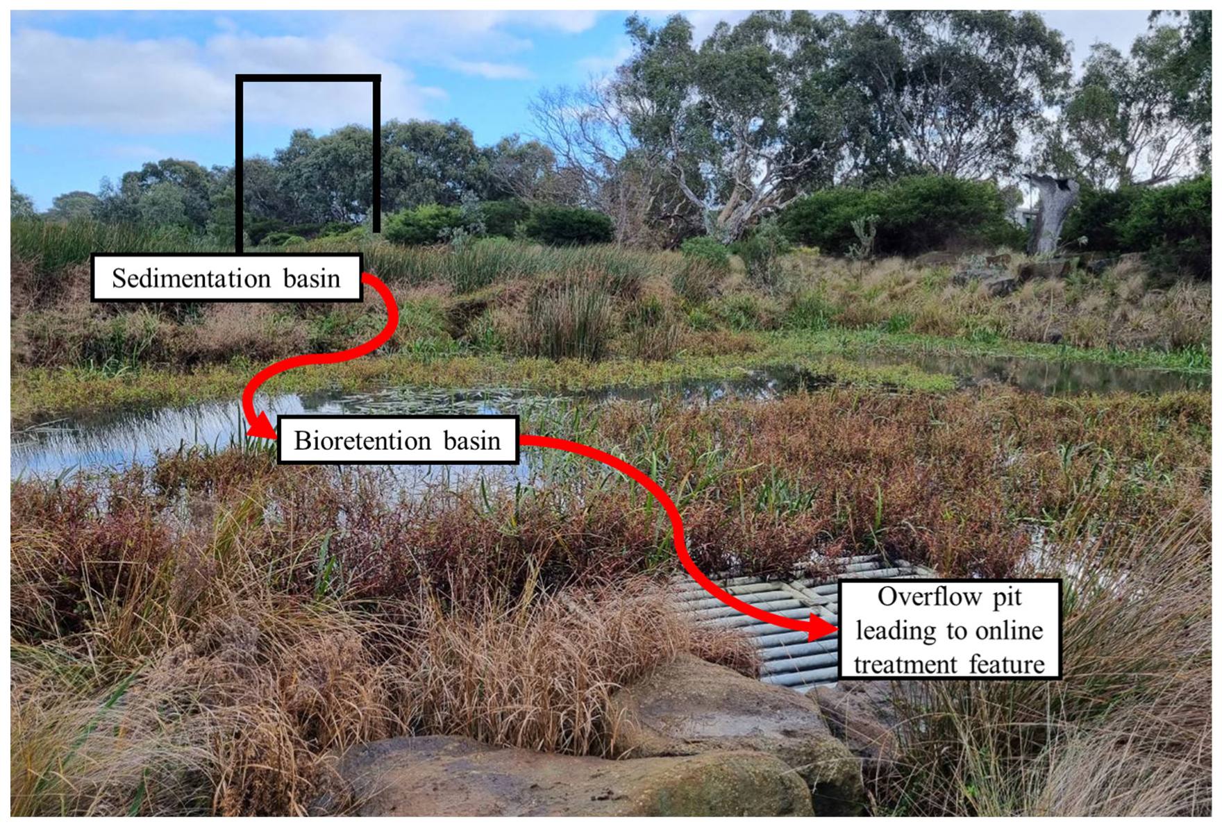
The Sparrovale Water samples were collected in the Armstrong Creek catchment between 29 May and 19 July 2024, with sampling locations strategically selected to include both the online treatment features of the Armstrong Creek cascading wetland system and an offline treatment feature, allowing for an assessment of the cumulative treatment effects and the role of each configuration in improving water quality. Sampling for the online treatment features covered four sites located along the longitudinal axis of the cascading wetland system, with samples collected from the online NbS ponds/wetlands. These sample sites, spaced at approximately 700 m intervals, include UP-ON, which captures water quality at the upstream online feature; MID-ON, corresponding approximately to the midpoint between UP-ON and DS-ON; DS-ON, representing the downstream online feature; and ARM-DIS, marking the final discharge point of the cascading wetland system (Figure 1). For the offline treatment feature, two sample sites were collected, one (IN-OFF) from an outlet of a 5.7 ha residential catchment into a sedimentation basin, and one (OUT-OFF) near the outlet of the bioretention basin that receives flow from the upstream sedimentation basin (Figure 1a and Figure 4). The two basins are designed to be hydraulically connected as an offline treatment system with runoff discharge into the cascading wetland system through an overflow pit structure (Figure 4).

Figure 4. Example of sedimentation and bioretention basins operating as an offline treatment system for a residential catchment in Armstrong Creek.

Since wetlands are generally designed for a 72 h residence time, wet weather samples at each site were collected over three consecutive 24 h periods following the end of a rainfall event. The study covered four storm events, resulting in a total of 66 samples for wet weather analysis. In addition to the wet weather samples, two dry weather sampling events (≥3 days with no rainfall prior to sampling) were conducted to establish background concentrations, providing a total of 12 samples from the six sampling points. Grab samples were collected from each site using a dipper that was pre-rinsed with water from the respective sampling location to minimize cross-contamination. Samples were then stored in a high-density polyethylene (HDPE) bottle pre-rinsed with distilled water, placed in a chiller box, transported to the laboratory in the School of Engineering at Deakin University, and refrigerated until testing. The samples were tested for Total Suspended Solids (TSS), Total Nitrogen (TN), and Total Phosphorus (TP) using standard methods [57] as follows:

• TSS, Method 2540 D determined by gravimetric filtration using Westlab 663–350 glass microfiber filters (nominal pore size: 1.2 µm, diameter: 47 mm, and thickness: 0.26 mm; Westlab, Ballarat, VIC, Australia), with a detection limit of 2.5 to 200 mg/L.
• TN, Method 10071 (Persulfate Digestion Method), analyzed using a HACH DR3900 Laboratory Spectrophotometer (HACH, Dandenong South, VIC, Australia) programmed with 350 N, Total LR TNT, with a detection limit of 0.5 to 25 mg/L.
• TP, Method 8190 (USEPA¹PhosVer^® 3 with Acid Persulfate Digestion Method), analyzed using the same spectrometer as for TN, but programmed with 536 P Total/AH PV TNT, with a detection limit of 0.06 to 3.5 mg/L PO₄³⁻.

2.2.2. Geelong Catchment Water Quality Data

Existing water quality datasets (Table 1) from earlier research projects in different catchments of the Geelong area were included in this study to understand general water quality characteristics at a broader catchment scale. A total of 545 water quality samples from 58 events were reported for the period July 2017 to April 2025, primarily from residential catchments, and analyzed for TN, TP, and TSS. These samples were collected as part of ongoing studies within the Greater Geelong area, with some datasets already published and some remaining unpublished (See Table 1). Samples from Grovedale, Bellarine, Corio, Rita Court A/B, and Warralily were collected using a level-actuated automated sampler, with samples obtained at discrete points in drainage pipes and at time intervals ranging from 5 to 40 min. However, sampling for Armstrong Creek was conducted using a grab sampling approach, with samples representing runoff from various land uses across the catchment, including residential, construction, farmland, and open spaces, collected in ponds/wetlands after rain events, and are considered as integrated for the whole event.

Table 1. Summary of past data for the Geelong catchment area.

Sampling Sites	Distance from Study Catchment	Area (ha)	Date	Events	Total Samples	Parameter Analyzed	References
Grovedale *	1 km	41.6	24 October 2022– 13 November 2022	4	56	TN, TP, TSS	Geelong Water Quality Monitoring Dataset [58]
Bellarine *	6 km	15.7	22 October 2017– 24 March 2018	9	87	TN, TP, TSS	Dharmasena et al. [12]
Corio *	15 km	41	23 July 2017– 23 August 2017	6	64	TN, TP, TSS	Geelong Water Quality Monitoring Dataset [58]
Rita Court A, B *	12 km	4.1,7	17 October 2018– 7 October 2019	8	65	TN, TP, TSS	Dharmasena et al. [12]
Warralily *	Within the catchment	85.2	1 December 2017– 2 May 2021	14	171	TN, TP, TSS	Dharmasena et al. [12]
Armstrong Creek **	Within the catchment	20–184 (8 sites)	16 March 2025– 2 April 2025	17	102	TSS	Armstrong Creek Water Quality [59]
This Study **	n/a (6 sites)	n/a (6 sites)	29 May 2024– 19 July 2024	13	78	TN, TP, TSS

Note: * refers to sampling using an automated pump sampler; ** refers to sampling using the grab sampling method.

Table 1. Summary of past data for the Geelong catchment area.

Sampling Sites	Distance from Study Catchment	Area (ha)	Date	Events	Total Samples	Parameter Analyzed	References
Grovedale *	1 km	41.6	24 October 2022– 13 November 2022	4	56	TN, TP, TSS	Geelong Water Quality Monitoring Dataset [58]
Bellarine *	6 km	15.7	22 October 2017– 24 March 2018	9	87	TN, TP, TSS	Dharmasena et al. [12]
Corio *	15 km	41	23 July 2017– 23 August 2017	6	64	TN, TP, TSS	Geelong Water Quality Monitoring Dataset [58]
Rita Court A, B *	12 km	4.1,7	17 October 2018– 7 October 2019	8	65	TN, TP, TSS	Dharmasena et al. [12]
Warralily *	Within the catchment	85.2	1 December 2017– 2 May 2021	14	171	TN, TP, TSS	Dharmasena et al. [12]
Armstrong Creek **	Within the catchment	20–184 (8 sites)	16 March 2025– 2 April 2025	17	102	TSS	Armstrong Creek Water Quality [59]
This Study **	n/a (6 sites)	n/a (6 sites)	29 May 2024– 19 July 2024	13	78	TN, TP, TSS

Note: * refers to sampling using an automated pump sampler; ** refers to sampling using the grab sampling method.

2.3. Development of Catchment Water Quality Model and Data Used

The flow model developed specifically for the Sparrovale Catchment by Teang et al. [51] was used in this study. Hydrologic and hydraulic processes governing inflows from the contributing catchment were simulated using PCSWMM (Personal Computer Stormwater Management Model, version 7.6.3665) employing the dynamic wave equation for runoff and flow routing estimates. Simulation timesteps were set at 30 s for dry and wet weather conditions, with a routing timestep of 1 s and a reporting interval of 1 h. The model included detailed representations of existing stormwater management infrastructure, such as underground pipes and pits, drainage channels, and ponds/wetlands that regulate runoff and flow within the catchment, along with hydraulic structures, control gate systems, and gate management operations that control peak runoff and flow distribution into Sparrovale Wetland and the downstream wetland complex. The model was calibrated using hourly observed water level data from three monitoring locations: Horseshoe Bend Linear Wetland Outlet, Balog Channel Outlet, and Sparrovale Wetland over a 30-month period spanning from May 2022 to October 2024. The calibration results of all sites varied from 0.55 to 0.79 for the Nash–Sutcliffe Efficiency (NSE) and from 0.8 to 0.89 for the Coefficient of Determination (R²), offering a reliable representation of hydraulic/hydrologic conditions needed for water quality modeling.

Following the methodology of Teang et al. [51], the meteorological inputs used to drive the water quality model included rainfall at 1 min intervals and daily evapotranspiration data over a 12-month period from October 2023 to September 2024, both derived from the Breakwater (Geelong) Racecourse weather station, located approximately 5 km from the study catchment (station ID: 87184, 38°10′11.93″ S, 144°22′48.02″ E). Rainfall at the station was recorded using a tipping bucket rain gauge [55], while reference evapotranspiration was estimated using the Penman–Monteith method [56]. The model was validated using the observed Sparrovale water quality dataset collected in the Armstrong Creek between May and July 2024. Within PCSWMM, an exponential buildup/washoff approach was used to estimate pollutant loading from the urban/residential catchment, while the Modified Universal Soil Loss Equation (MUSLE) was applied to estimate sediment loading from construction sites, agricultural areas, and open spaces. Selecting a model application capable of simulating these distinct, dynamic, land-use-based processes in an integrated manner is critical. Although alternative water quality models exist, most do not represent these dynamic processes simultaneously, at short time steps, with a typical subsurface urban drainage network (e.g., Soil and Water Assessment Tool (SWAT), Agricultural Non-Point Source (AGNPS), and Water Erosion Prediction (WEPP) models) [60,61,62], especially for long-term continuous simulations. Among the models reviewed, DR3M-QUAL and SWMM-based applications share a similar conceptual foundation, simulating both runoff generation and pollutant transport within an integrated framework. However, DR3M-QUAL is best suited for small urban areas, with limitations including the inability to model pollutant interactions and weak sediment transport simulation, except in storage basins [9]. Most importantly, the model has not been maintained or recently updated, resulting in a lack of advanced algorithms, numerical stability, and modern software support, unlike SWMM-based model applications. Zong et al. [63] coupled SWAT and SWMM to represent water quality for a mixed land-use catchment in Liaoning Province of northeastern China, but this necessitated the coupling of two models. PCSWMM, built on EPA’s Storm Water Management Model (SWMM), allows for the seamless combination of various simulation components such as hydraulic/hydrologic modeling, buildup/washoff modeling, erosion modeling, and LID (Low Impact Development) features [64]. Thus, our water quality models were integrated directly into the existing catchment flow model developed by Teang et al. [51]. The buildup/washoff model for the urbanized areas of the catchment was estimated using the following Equations (1) and (2):

B = C₁ (1 − e − C₂^t)

(1)

W = C₃q^c₄B

(2)

where B = pollutant buildup (kg/ha), W = pollutant washoff (kg/ha), C₁ = maximum buildup possible (kg/ha), C₂ = rate constant (1/day), C₃ = washoff coefficient, C₄ = washoff exponent, and q = runoff rate per unit area (mm/h).

All ponds/wetlands were represented as 1-D storage units, each defined by a storage curve describing the elevation and volume relationship, as developed in Teang et al. [51]. The reduction of TN, TP, and TSS within these storage units was scripted in PCSWMM using an exponential decay function, given in Equation (3):

C_o = C* + (C_i − C*) e^{−ki (Δt/D)}

(3)

where C_o, C_i, and C* represent the outlet, inlet, and background concentrations for TN, TP, and TSS in mg/L, respectively. The background concentration (C*) was calculated from water quality data collected during dry weather events. A unique decay constant, k_i (m/h), for each pollutant (k_TN = 0.089, k_TP = 0.061, k_TSS = 0.126) was derived from Dharmasena et al. [12]. Given that the study was conducted in an upstream wetland of the cascading wetland system, and all wetlands are generally designed for a 72 h hydraulic residence time, the decay values are considered applicable to the entire cascade. Δt is the computational time step (h), and D is the water depth (m) at time t (h) in the storage unit.

Williams [65] developed the MUSLE as a watershed-based model to estimate sediment yield from individual storm events. This modified version of the USLE model replaced the rainfall factor in the original USLE with a runoff factor, which is considered a better indicator of the energy available for sediment detachment and transport on a storm event basis. The MUSLE uses runoff volume (Q_surf, mm) and peak runoff rate (q_peak, m³/s) along with other standard USLE parameters, including soil erodibility (K, t ha h ha⁻¹ MJ⁻¹ mm⁻¹), slope steepness and length (LS), cover management (C), and conservation practices (P) to estimate erosion from subcatchments. Runoff volume and peak runoff rate are determined by the PCSWMM hydrologic calculations. The model also incorporates a coarse fragment factor (CFRG) and uses location coefficients “a” and “b”, with default values of 11.8 and 0.56, respectively, in scaling predictions to match different local conditions. Parameter values used for erosion modeling in this study are summarized in Table 2. Among these parameters, only the C value for construction sites and the p value were adjusted for catchment conditions to better represent site-specific ground cover dynamics and erosion control. The value for K was based on local soil data and Teng et al. [36], while LS was determined from the size of the catchment and the lidar-derived DEM data with 1 m spatial resolution and 0.1 m vertical accuracy. The C factor, which measures the type and extent of ground cover that protects soil from erosion, generally is lower for wetland and vegetated surfaces compared to more exposed surfaces such as bare areas and construction sites. C values for wetlands, vegetated areas, and bare soils were fixed based on established literature, representing more stable surface covers, unlike construction sites, which can have values as high as 1, reflecting their disturbed and exposed conditions during construction (Table 2). Similarly, the P factor accounts for the effects of soil conservation practices such as contour farming, terracing, or other erosion control measures in reducing erosion. The MUSLE applied in this context is given in Equation (4):

Sediment Yield (Mg/day) = a × (Q_surf × q_peak × Area) ^b × K × C × P × LS × CFRG

(4)

Table 2. Parameter values for erosion modeling in this study.

Parameters	Values	References/Descriptions
Qsurf (mm)	–	Calculated dynamically within PCSWMM; explicit values are not reported.
qpeak (m3/s)	–	Calculated dynamically within PCSWMM; explicit values are not reported.
K (t ha h ha−1 MJ−1 mm−1)	0.026	Teng et al. [36]
C
Wetland	0.05	Yang et al. [66]
Grassland	0.06	Yang et al. [67]
Rangland/pasture	0.08	Yang et al. [67]
Bare areas	0.35	Yang et al. [66]
Construction site	1	Wischmeier and Smith [23]
P	0.5	Wischmeier and Smith [23].
LS	0.28–25	Determined based on catchment geometry and DEM data
CFRG	0.99	Hu et al. [47]

Table 2. Parameter values for erosion modeling in this study.

Parameters	Values	References/Descriptions
Qsurf (mm)	–	Calculated dynamically within PCSWMM; explicit values are not reported.
qpeak (m3/s)	–	Calculated dynamically within PCSWMM; explicit values are not reported.
K (t ha h ha−1 MJ−1 mm−1)	0.026	Teng et al. [36]
C
Wetland	0.05	Yang et al. [66]
Grassland	0.06	Yang et al. [67]
Rangland/pasture	0.08	Yang et al. [67]
Bare areas	0.35	Yang et al. [66]
Construction site	1	Wischmeier and Smith [23]
P	0.5	Wischmeier and Smith [23].
LS	0.28–25	Determined based on catchment geometry and DEM data
CFRG	0.99	Hu et al. [47]

2.4. Variability of Washoff and Erosion Model Parameters

In assessing the uncertainty of buildup/washoff model parameters and impact on pollutant load estimates, this study focuses on the washoff parameters, C₃ and C₄, as they tend to produce greater variability due to their sensitivity to local factors such as rainfall intensity and surface characteristics, compared to the buildup parameters, C₁ and C₂, which are largely governed by spatially uniform factors such as land use and climate [14,68] and are therefore fixed, adopting the values obtained by Dharmasena et al. [12]. A total of 11 washoff parameter sets for TN, TP, and TSS were obtained from Chaudhary et al. [11], which specifically had been calibrated for the Geelong area, with five corresponding to the Bellarine and six to the Rita Court dataset (Table 3). Although the Geelong dataset may be considered appropriate for the Sparrovale catchment, as these are catchments with similar characteristics, there is uncertainty regarding the model parameters to use since the parameter sets differ between events. These eleven parameter sets were therefore incorporated in our water quality model to evaluate the range of pollutant concentrations and loads expected under different parameterizations. Following this approach, it will be able to assess the uncertainty in model predictions due to variability in washoff parameters.

Table 3. Washoff parameter sets for the Geelong area from Chaudhary et al. [11].

Catchments		TN		TP		TSS
		C3	C4	C3	C4	C3	C4
Bellarine	15 November 2017	0.003668	2.74	0.002375	2.116	0.007153	1.742
	12 January 2018	0.5548	0.7125	0.3749	0.4396	0.09116	1.823
	13 January 2018	1.939	1.018	0.9214	0.5455	0.9707	0.2891
	19 February 2018	0.9699	0.7621	0.003248	0.948	0.9557	1.127
	22 October 2017	0.01291	1.489	0.01621	1.217	0.8497	2.38
Rita Court	12 December 2018	0.4125	0.6644	0.1228	1.175	0.1217	1.17
	17 October 2018	0.004516	1.08	0.759	1.338	0.02184	1.549
	22 November 2018	1.225	1.129	0.02628	1.103	1.288	1.22
	5 September 2019	0.8279	1.31	0.7864	1.797	0.8797	2.817
	15 September 2019	0.5972	1.066	0.01803	1.091	0.01161	0.9529
	8 August 2019	0.4669	0.3112	0.1852	0.5448	0.7625	0.2349

Table 3. Washoff parameter sets for the Geelong area from Chaudhary et al. [11].

Catchments		TN		TP		TSS
		C3	C4	C3	C4	C3	C4
Bellarine	15 November 2017	0.003668	2.74	0.002375	2.116	0.007153	1.742
	12 January 2018	0.5548	0.7125	0.3749	0.4396	0.09116	1.823
	13 January 2018	1.939	1.018	0.9214	0.5455	0.9707	0.2891
	19 February 2018	0.9699	0.7621	0.003248	0.948	0.9557	1.127
	22 October 2017	0.01291	1.489	0.01621	1.217	0.8497	2.38
Rita Court	12 December 2018	0.4125	0.6644	0.1228	1.175	0.1217	1.17
	17 October 2018	0.004516	1.08	0.759	1.338	0.02184	1.549
	22 November 2018	1.225	1.129	0.02628	1.103	1.288	1.22
	5 September 2019	0.8279	1.31	0.7864	1.797	0.8797	2.817
	15 September 2019	0.5972	1.066	0.01803	1.091	0.01161	0.9529
	8 August 2019	0.4669	0.3112	0.1852	0.5448	0.7625	0.2349

In erosion modeling, uncertainty commonly is associated with the C and P factors [23]. While C is dynamic in agricultural systems, this study focused more on construction sites, where temporary disturbances can cause severe localized erosion [47]. In part, this focus was driven by our field observations. A C value of 1 is used to represent active construction, but can be decreased to 0.15 for actively managed sites [69]. For the assessment of erosion variability in the catchment, two scenarios were tested: (Min. bound) C assigned a value of 0.15 for construction sites with P remaining at 0.5, and (Max. bound) C values unchanged but P set to 1 for all pervious land subject to erosion. In consideration of the greater certainty with respect to the erosion driving factors, our analysis of erosion model variability was limited to TSS.

3. Results and Discussion

3.1. Characterization of Stormwater Quality for Catchments in Geelong

Table 4 presents stormwater quality data from the various catchments across the Geelong area, collected between July 2017 and April 2025. The data from each catchment were pooled and analyzed to derive the average ± standard deviation (SD) values for TSS, TP, and TN, and compared to assess the spatial variability of pollutant concentrations at a broader catchment scale. Among the catchments, Corio recorded the highest mean concentrations of TSS (237 ± 177 mg/L) and TP (2.66 ± 1.08 mg/L), while Bellarine had the highest TN (3.95 ± 2.08 mg/L). High TSS accompanied by high TP can reflect the particulate-bound nature of phosphorus transport commonly observed in urban runoff [5]. Standard deviations were high relative to the mean, indicating considerable variability in concentrations during the sampling period. Similar patterns were observed in other catchments, including Grovedale, Rita Court, and Warralily, though with generally lower constituent levels, reflecting storm event-driven dynamics typical of urban catchments, where washoff is strongly influenced by antecedent dry periods, storm intensity, and rainfall volume [5,11].

Table 4. Water quality data across different catchments in Geelong area (mg/L).

Catchment		TSS		TP		TN
		Average	SD	Average	SD	Average	SD
Grovedale		35	25	0.88	0.28	4.0	2.1
Bellarine		64	77	1.4	1.1	5.7	5.0
Corio		237	177	2.7	1.1	n/a	n/a
Rita Court		84	54	1.1	0.45	3.8	1.9
Warralily		97	88	1.0	0.75	3.4	3.0
Armstrong Creek		61	21	n/a	n/a	n/a	n/a
This Study, Sparrovale Catchment:
Online treatment system	UP-ON	11	15	0.64	0.83	1.3	0.9
	MID-ON	4.0	3.5	0.38	0.18	0.57	0.94
	DS-ON	7.2	6.6	0.39	0.12	0.91	1.23
	ARM-DIS	50	12	0.49	0.24	1.7	1.1
Offline treatment system	IN-OFF	3.5	3.7	0.42	0.21	0.92	0.77
	OUT-OFF	6.0	5.4	0.32	0.20	1.2	1.2

Note: n/a refers to values that are not available.

Urban runoff in Australia often contains TSS levels ranging from 20 to 1000 mg/L, TN from 0.6 to 8.6 mg/L, and TP from 0.12 to 1.6 mg/L [70]. These values considerably exceed the recommended levels of ≤25 mg/L for TSS, ≤0.5 mg/L for TN, and ≤0.05 mg/L for TP by O’Loughlin [71], reflecting high TSS and nutrient concentrations associated with urban runoff in the country. The National Committee on Water Engineering later adopted these limits as reference concentrations for managing urban stormwater in Australia, as documented in Australian Runoff Quality—A Guide to Water Sensitive Urban Design [72]. Observed TSS and nutrient concentrations in the Geelong catchments (Table 4) generally are consistent with the typical Australian urban runoff quality ranges and exceed the recommended levels. The results also fall within or exceed the trigger values that can potentially harm aquatic ecosystems in wetland environments (2–80 mg/L TSS, 0.6–1.5 mg/L TN, and 0.03–0.08 mg/L TP), as published in the Australian and New Zealand Guidelines for Fresh and Marine Water Quality [73]. High TN and TP levels imply that the catchment already is at risk of eutrophication. In particular, Irvine and Murphy [74] in a survey of the literature, reported that the boundary between mesotrophic and eutrophic conditions should lie within 0.3–1.5 mg/L for TN and 0.042–1 mg/L for TP; therefore, even moderate nutrient levels, particularly near the upper bounds of these thresholds, can be a concern for sensitive receiving ecosystems. The extreme TP level at Corio during the sampling period highlights that the catchment may function as a nutrient hotspot. Follow-up monitoring at Corio will be crucial in tracking the sources and planning mitigation measures.

3.2. Characterization of Stormwater Quality in the Sparrovale Catchment

Water quality data for the Sparrovale catchment (see Table 4), in general, exhibited low concentrations of TSS, TN, and TP compared to the other sites in the Geelong area, as assessed from the offline and online monitoring sites in the Armstrong Creek cascading wetland system. While this provides regional context across the broader catchment, direct numerical comparison is limited by differences in temporal resolution arising from the difference in sampling method (automated vs. grab sampling). Within the Sparrovale system, a clear spatial variation was observed in the downstream direction of the online sites, with mean concentrations declining from the upstream online ponds/wetlands (UP-ON) through the midstream (MID-ON) and downstream (DS-ON) locations, before increasing markedly near the outlet (ARM-DIS) of the cascading wetland system. TSS, in particular, increased nearly fivefold as measured at the ARM-DIS (50.1 ± 11.6 mg/L) compared to the furthest upstream site, UP-ON (11.34 ± 15.48 mg/L) (Table 4). Field observations revealed that the downstream area of the Sparrovale catchment is characterized by extensive open spaces, agricultural areas, and construction projects, which potentially contribute to high sediment levels in runoff. Subsequent monitoring showed consistently high TSS concentrations (61 ± 21.2 mg/L) at the ARM-DIS site and nearby areas in the Sparrovale catchment affected by construction [59]. The considerable reduction of mean TSS, TP, and TN levels by 65%, 41%, and 55%, respectively, between the UP-ON and MID-ON sites illustrates the potential role of the cascading wetland system for sedimentation and nutrient uptake. However, the increase of mean concentrations at the outlet (ARM-DIS) from the DS-ON site by 600% for TSS, 26% for TP, and 84% for TN indicates a potential discharge of new TSS and nutrients from the open spaces, agricultural areas, and in particular, the construction sites, as noted. Given the observed variability in the water quality data collected for the Sparrovale catchment, t-tests were applied to explore the significance of change between sites. Results revealed that there are differences between the UP-ON and MID-ON although with different levels of uncertainty (p = 0.065 for TSS, 0.16 for TP, and 0.06 for TN), consistent with the calculations of reduction in mean concentration between sites. The difference between DS-ON and ARM-DIS sites was significant for TSS (p ≤ 0.05) and suggestive for TP and TN (p = 0.09 and 0.08, respectively), indicating the potential influence of the contributing land uses and construction on increased TSS and nutrient levels, consistent with the calculations of percent increase in mean concentrations.

The effect of the offline treatment system remains unclear. Based on our sample results, the value of p was 0.1, 0.23, and 0.12 for TSS, TN, and TP, respectively, indicating a general lack of significant difference between mean inlet and outlet levels. While bioretention systems have been widely implemented to manage urban runoff, their performance in terms of pollutant removal can vary by site and pollutant. Lucke and Nichols [75], in their assessment of five bioretention basins for road runoff treatment, reported that although the basins helped remove TP, increased TSS and TN levels suggest bioretention basins as contributing sources of sediment and TN to the downstream aquatic environment. Mangangka et al. [76] assessed the performance of a bioretention basin for residential runoff management and found that the basin performed well in controlling TSS levels, but generally produced negative results for TP and TN. Higher TP and TN levels at the discharge of the bioretention basin were associated with the occurrence of nutrient leaching from the filter media, which may have been produced by the flushing of nutrients retained from prior events and the release of nutrients present in the media itself. Irvine et al. [77] noted that the common design of bioretention systems with sandy filter media allows for quick drainage but has low carbon content, creating unfavorable conditions for microbial denitrification, which limits the conversion of nitrate to nitrogen gas released into the atmosphere, although this can be addressed by the addition of a carbon source, such as woodchips. Our field measurement data indicate that the offline treatment system may have to be visited for maintenance, and subsequent monitoring would indicate whether the bioretention system remains efficient in treating runoff. In addition, incorporating detailed hydrological/hydraulic and water quality modeling would provide insights into system performance optimization under varying rainfall conditions. This is particularly important given that the performance of bioretention systems depends on rainfall characteristics as well as inflow and outflow discharge [76].

3.3. Water Quality Model Results for Sparrovale Catchment

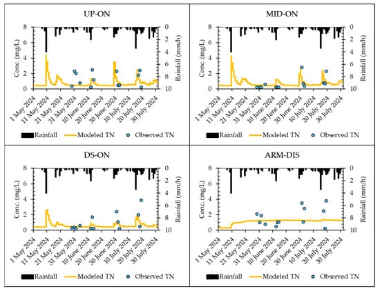
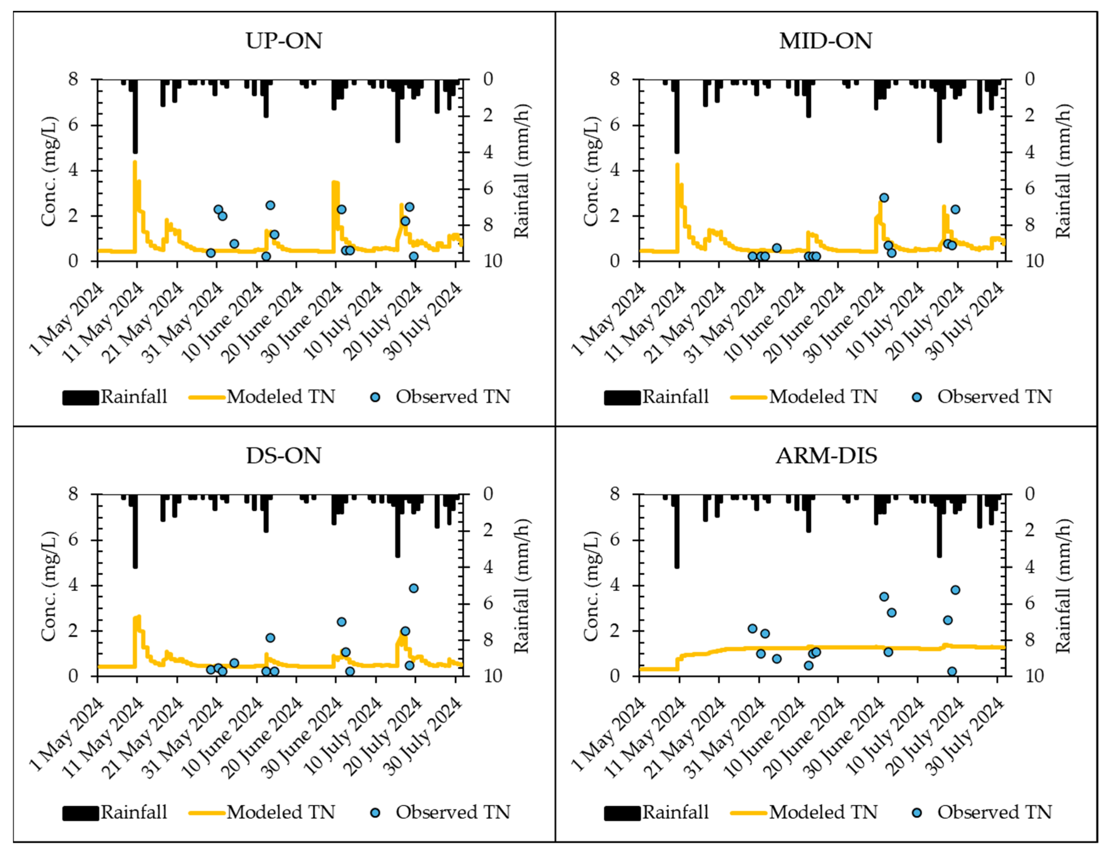
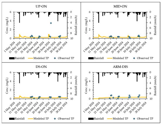
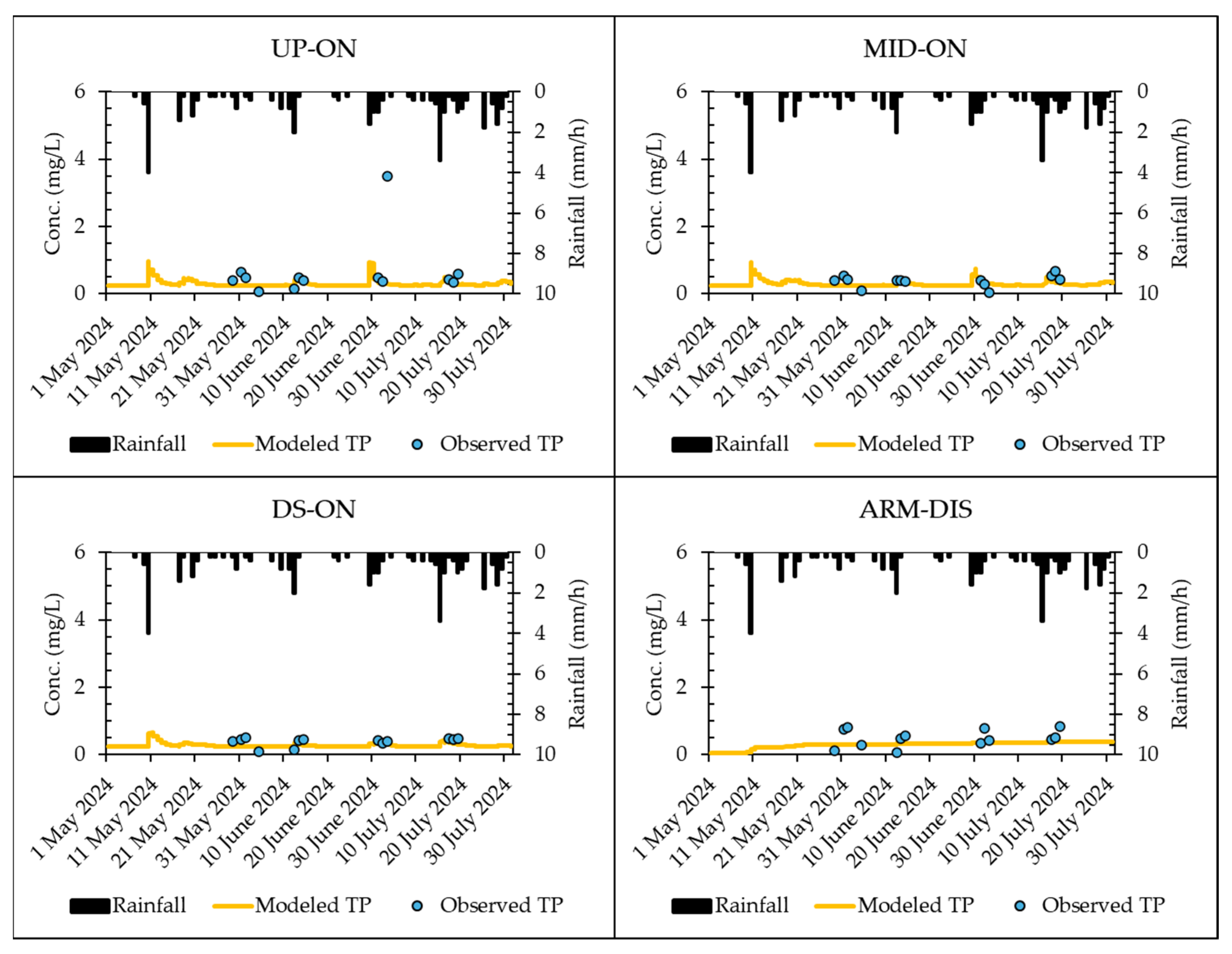
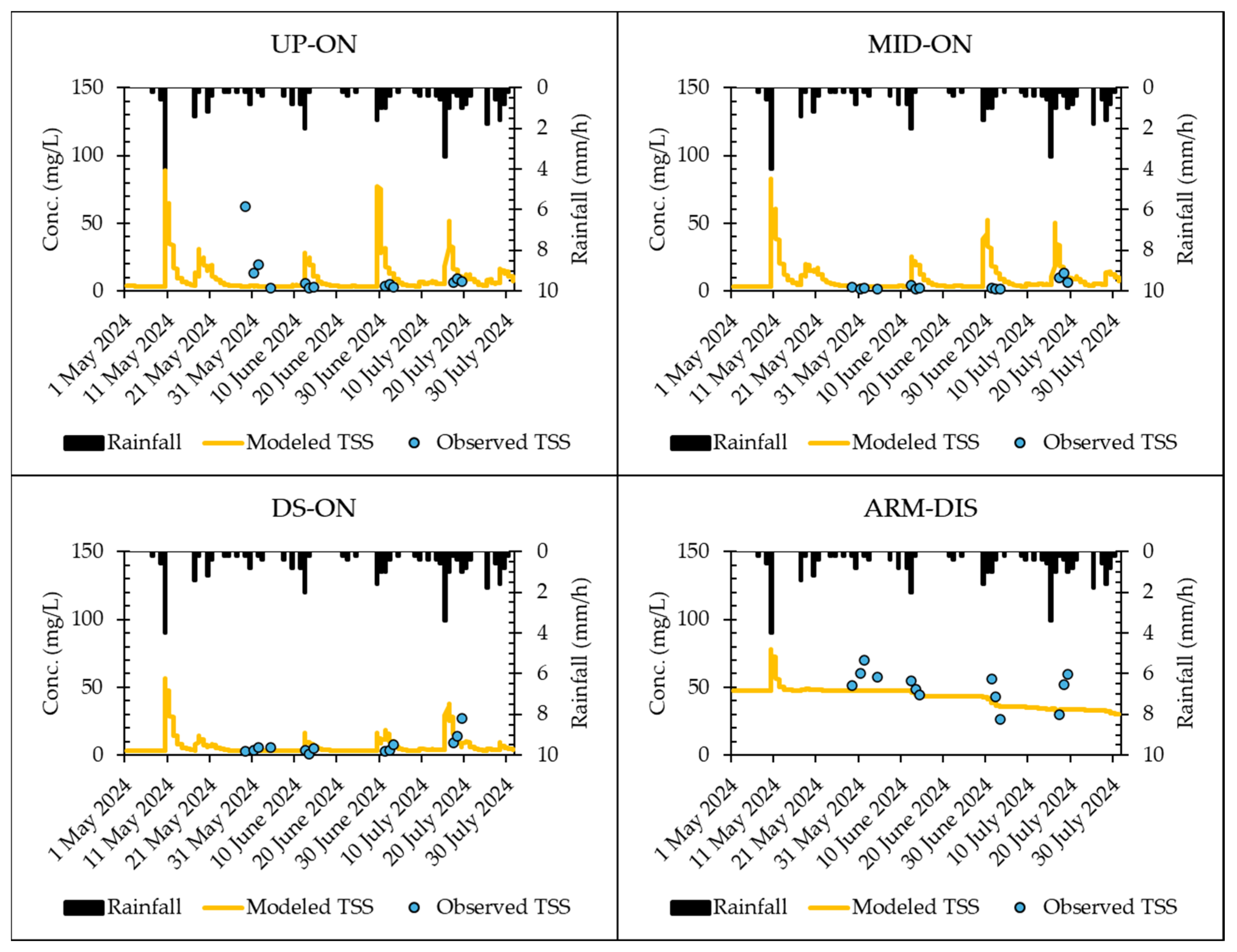
Reference water quality analysis was modeled using the buildup/washoff model parameters determined by Dharmasena et al. [12] for Warralily, a site located within the Sparrovale catchment, based on a limited number of storm events, and incorporating the erosion model with C and p values optimized for fit (Table 2) based on catchment conditions. Figure 5, Figure 6 and Figure 7 present the model results for TN, TP, and TSS levels compared to observed data for the online monitoring sites (UP-ON, MID-ON, DS-ON, and ARM-DIS) for the May–July period, corresponding to the availability of observed water quality data used for model validation. Due to the periodic nature of the observed water quality data and the limited number of storm events noted, quantitative goodness-of-fit assessments against continuous model predictions are not conducted. Such metrics could be dominated by temporal sampling gaps, fail to capture short-duration pollutant pulses, and provide statistically uncertain evaluations given the sparsity of our observed data. Overall, the model reasonably reproduces the observed pollutant concentrations, given the inherent variability of urban runoff water quality and the difficulty in catchment water quality modeling [10], particularly the complex processes involved in predicting pollutant concentrations and their dynamics [78]. In predicting TN and TP (Figure 5 and Figure 6), the model provided reasonable estimates across all locations using the buildup/washoff parameters obtained by Dharmasena et al. [12] for a smaller urban land use catchment with similar characteristics, despite the inherent variability and complexity of runoff quality prediction noted above. The modeled TSS concentrations agree well with the observed data (Figure 7), indicating that integrating buildup/washoff and erosion models is suitable in mixed-use, urbanizing catchments. Importantly, our model was able to capture the upstream-to-downstream water quality variations in the Armstrong Creek cascading wetland system well, including the attenuation of pollutants in the upstream reaches and the reintroduction of pollutants in the downstream area (as discussed in Section 3.2). The wetland model benefits from using the first-order decay approach, treating changes in water quality as a temporal, exponentially decaying process, which, despite its simplification, provides reasonable predictions for assessing the performance of the NbS cascade wetlands. Such NbS multi-stage configurations have been documented in other forms, including sequential constructed wetlands [79] and WSUD treatment trains linking raingardens and detention ponds [77,80]; however, the cascading wetland system in this study is analogous to the cascade reservoir system on the Lancang River, where hydrologically connected units operate in sequence to regulate downstream flow regimes [81]. Although each stage contributes to treatment, pollutant concentrations can increase in downstream reaches due to additional catchment inputs [82], consistent with our findings noted above (Section 3.2).

Figure 5. Comparison between modeled and observed TN for the cascading wetland system.

Figure 6. Comparison between modeled and observed TP for the cascading wetland system.

Figure 7. Comparison between modeled and observed TSS for the cascading wetland system.

From the results, TN and TSS (Figure 5 and Figure 7) exhibit a pronounced rainfall-driven response as shown from UP-ON through DS-ON concentrations, where peak concentrations increase with increased rainfall intensity, and decline toward background levels under low-flow or dry conditions. In contrast, TP showed a weaker response (Figure 6) to rainfall. During the simulation period from May to July 2024, the catchment experienced a maximum daily rainfall depth of up to 12 mm, with rainfall intensities ranging from 0.2 to 4 mm/h. As noted by Chaudhary et al. [11] with regard to temperate climates, TSS shows a clear relationship with rainfall depth when rainfall exceeds 5 mm/day; however, for smaller events, the buildup and washoff mechanisms of TSS primarily are driven by rainfall intensities. The relationship between levels of TN or TP and rainfall characteristics is weaker and weaker still for dissolved pollutants [11,83]. The strong response of TN to rainfall in this study (Figure 5) likely reflects the nature of our catchment, which contains a substantial proportion of agricultural land. Ekholm et al. [84] noted that agricultural land can release roughly ten times more TN than forested areas and other land uses, emphasizing the important contribution of farmland to nitrogen loading in the cascading wetland system. In their assessment of a river in southwest Finland, TN concentrations were found to correlate only with the percentage of agricultural fields, showing no correlation with field slopes.

Modeled results for TSS and nutrients at the ARM-DIS site, in general, show a relatively flat pattern with no clear response to changes in rainfall, while the observed data points tend to be more scattered and higher compared to the upstream sites (UP-ON through DS-ON). This suggests that the water quality dynamics at this particular location may not be entirely governed by the buildup/washoff and erosion processes that dominate the rest of the catchment. This discrepancy could be due to other factors that were not captured in the model, such as resuspension of pollutants from the stream bed [85], non-storm inflows, wind gusts, and other localized disturbances [70], including fish foraging and nest building [86,87]. These processes can introduce or redistribute TSS and nutrients independently of rainfall events, thereby reducing the accuracy of rainfall-driven models in predicting water quality.

3.4. Variability of Pollutant Levels Due to Uncertainty of Washoff Parameters

Stormwater runoff quality is subject to high variability due to uncertainty inherent in the buildup and washoff processes, which may not be fully captured by the C₁–C₄ coefficients [88]. In addition, variabilities across events, influenced by antecedent meteorologic conditions, particle size distribution and bulk density, and anthropogenic activities that may redistribute solids and adsorbed nutrients [16,17,18,89,90,91] lead to uncertainty in model parameters between events and further affects the interpretation and credibility of model results, particularly in ungauged areas that use parameters transferred from different watersheds with similar properties. Parameter uncertainty is considered one of the most important sources of error in water quality modeling [92,93]. Different parameter sets often can produce similar model results that match well with field data, making it difficult to identify a set that truly represents the physical reality of the system [94].

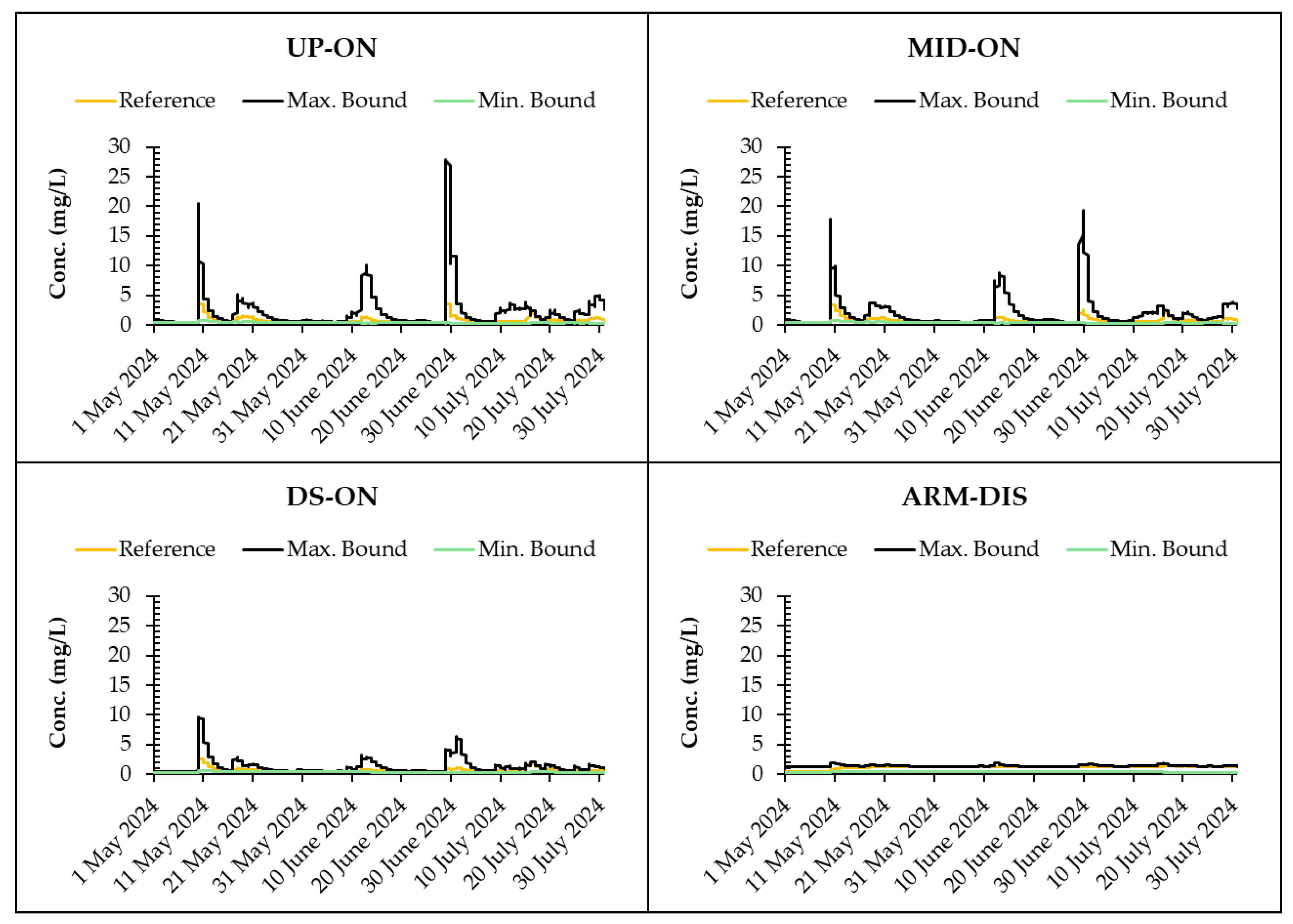
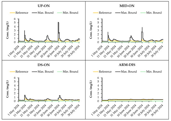
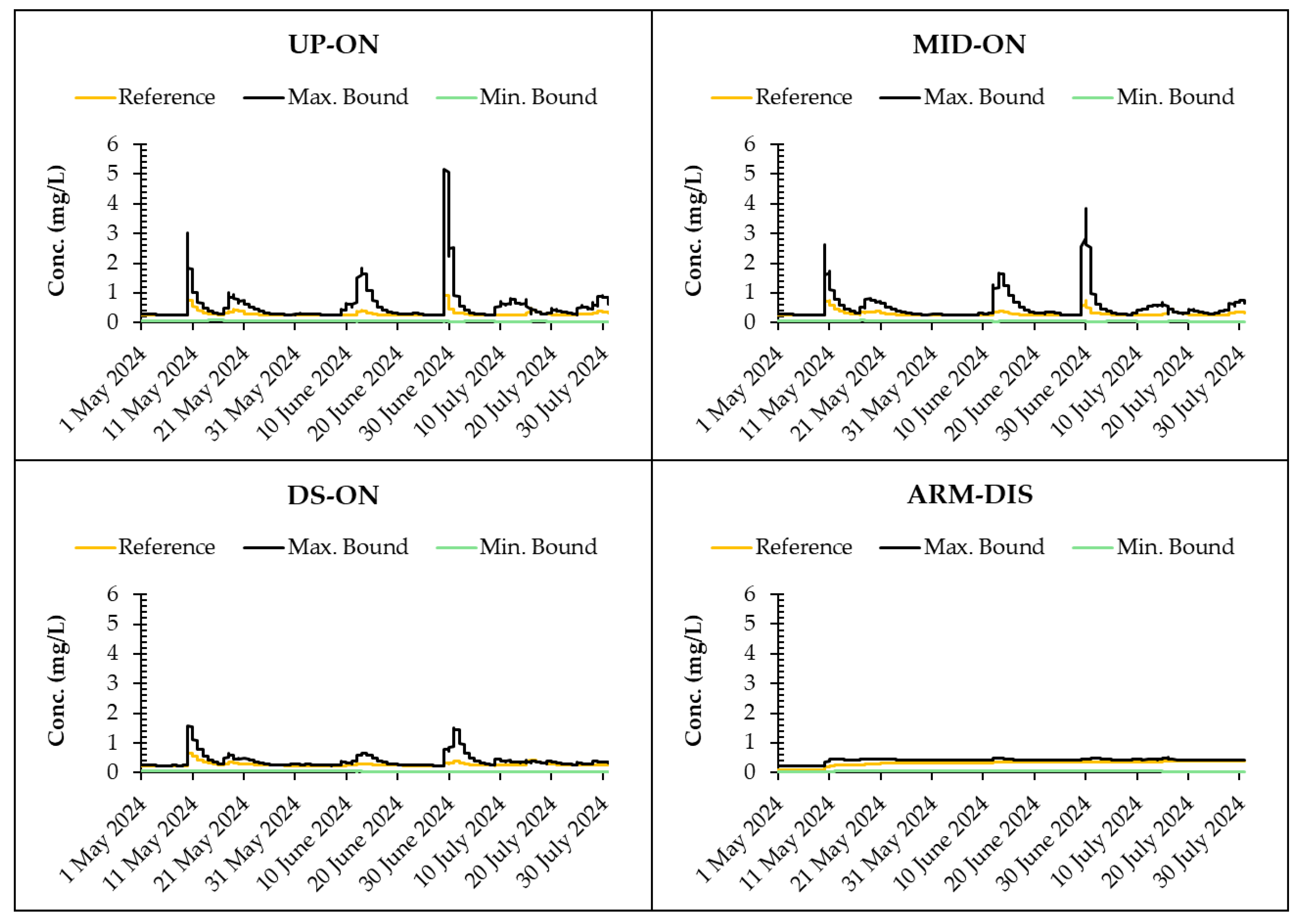
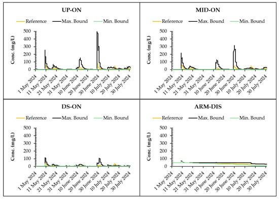
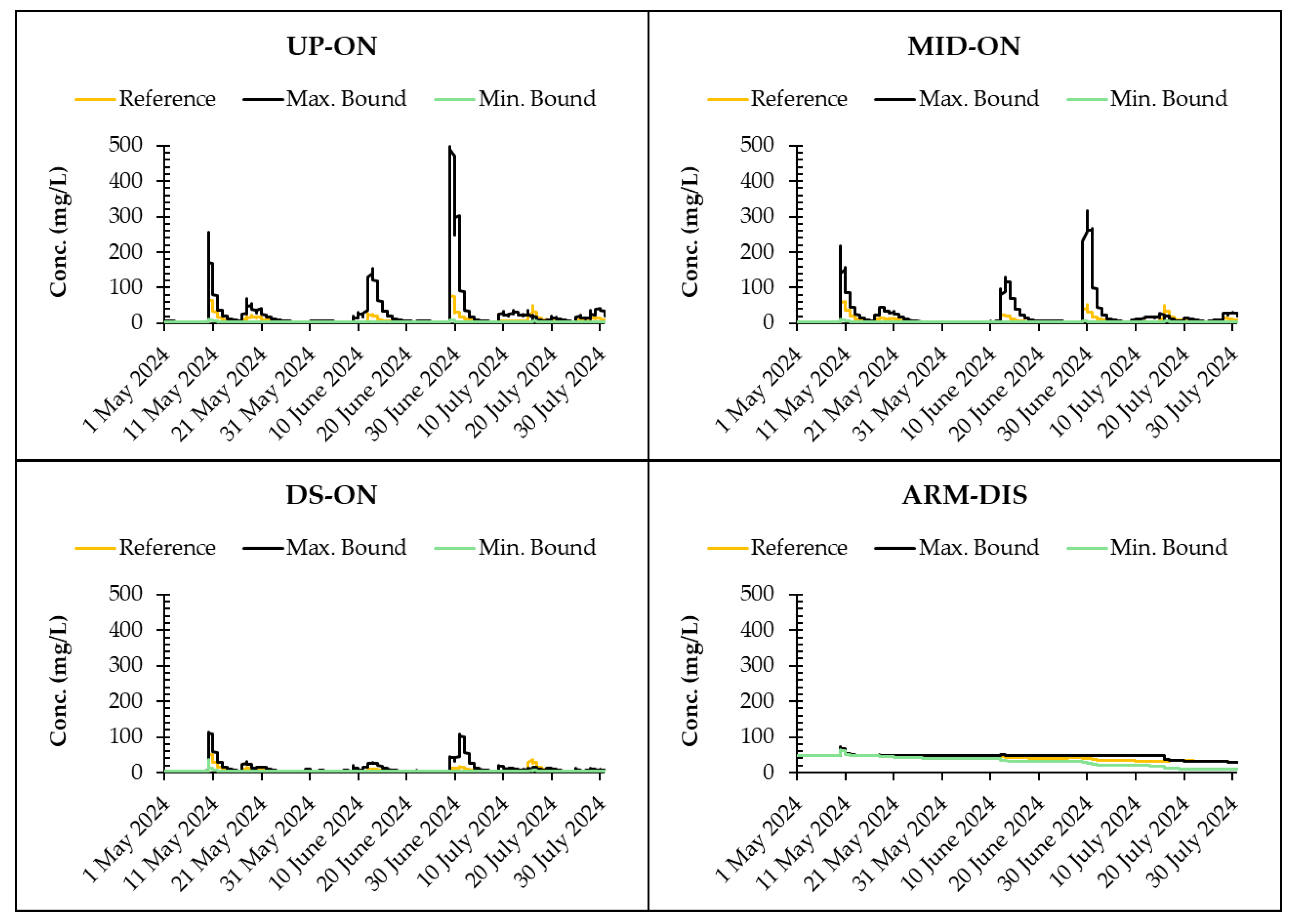
Figure 8, Figure 9 and Figure 10 illustrate the extent of uncertainty inherent in TN, TP, and TSS predictions arising from variability in the washoff parameter set. While a representative three-month period is shown to preserve temporal resolution and visual clarity, the uncertainty analysis was conducted over the full annual simulation period (October 2023 to September 2024), and similar patterns were observed throughout the year. Specifically, the figures highlight the results from the parameter sets that produced the minimum and the maximum bounds in the cascading wetland system. Although the uncertainty associated with the erosion model for TSS was evaluated for the C and P factors noted in the methodology (Section 2.4), results were similar to that produced in the reference model parameter set (see Figure 7) due to limited contribution of erosion observed in the comparison period (May to July 2024). Quantifiable erosion (7 events) occurred prior to this period, specifically on 24 November 2023 (30.2 mm/d); 25 November 2023 (6.8 mm/d); 9 December 2023 (20.2 mm/d); 8 January 2024 (23.4 mm/d); 17 January 2024 (13.2 mm/d); 1 April 2024 (40.8 mm/d); and 2 April 2024 (0.2 mm/d), with the values in parentheses representing the daily rainfall depth for each event. For most smaller storms, erosion played a negligible role compared to pollutant loads generated through washoff processes due to insufficient raindrop energy driving erosion from pervious surfaces [23]. However, during large events, erosion-driven sediment loads became dominant, greatly increasing total TSS levels at the downstream sites. From the results, the washoff parameter set producing the minimum bound was the calibrated set for Bellarine on 15 November 2017, while the set producing the maximum bound was from Bellarine on 13 January 2018 (see Table 3). The effect of C₃ and C₄ on pollutant washoff is driven by the distinct roles each parameter plays in the process. As noted by Chaudhary et al. [11], C₃ can vary by up to two orders of magnitude and is strongly influenced by rainfall, making it the primary factor controlling pollutant mobilization during storm events. C₄ varies over a limited range, affecting the rate of washoff based on local flow conditions rather than directly scaling the overall pollutant level. Therefore, a high C₃ value, due to its dominant influence on rainfall-driven pollutant transport, will inherently result in greater washoff regardless of the C₄ value. Results indicate that the upstream sites (UP-ON and MID-ON) exhibit the greatest sensitivity, characterized by substantial divergence between the maximum and minimum predicted concentrations, particularly during storm events. However, as we move downstream, and at the ARM-DIS site in particular, predicted concentrations of pollutants are less sensitive to the washoff dataset used for the entire simulation period (see Figure 8, Figure 9 and Figure 10). This suggests that the dynamics at this large, downstream wetland are not governed by the same rapid washoff processes that dominate the upstream sections, as noted in Section 3.3. The large volume of the wetland likely creates a long residence time, which buffers it from the short-term concentration spikes caused by rainfall.

Figure 8. Variability of TN level for the cascading wetland system.

Figure 9. Variability of TP level for the cascading wetland system.

Figure 10. Variability of TSS level for the cascading wetland system.

3.5. Variability of Pollutant Loads on the Uncertainty of Buildup/Washoff and Erosion Models

Table 5 provides yearly load estimates for TSS, TP, and TN from the Sparrovale catchment under the uncertainty in the buildup/washoff and erosion models. Table 5 shows that the Armstrong Creek catchment is expected to produce considerably greater TSS and nutrient load compared to the Horseshoe Bend, which is reasonable considering that the Armstrong Creek area is much larger. The pollutant load estimates from our reference model fall within the uncertainty ranges defined by changes in the buildup/washoff and erosion parameters. However, the buildup/washoff scenarios produced relatively small variations in load for TSS and nutrients from both subcatchments, suggesting a more stable prediction compared to the erosion scenarios. TSS under the erosion scenarios exhibit much higher variability in load, ranging from 1295 to 3010 Mg/year for Armstrong Creek and 78 to 186 Mg/year for Horseshoe Bend. This variation reflects changes in the C and P factors, indicating that sediment loads in the catchment are highly sensitive to land disturbance and erosion-control practices. Although Armstrong Creek is 3.3 times larger than Horseshoe Bend, the change in TSS loads due to erosion parameter variation was about 2.3 times in both catchments, suggesting that, despite their size difference, both systems respond proportionally to erosion processes. In predicting the sediment load, differences in hydrologic response between the two catchments further influence the magnitude of TSS loads. Small catchments can produce high sediment loads when rainfall intensity, hydrologic response, and the availability of erodible sediment are high, whereas larger catchments may yield less sediment when these factors are limited, suggesting that sediment load variability depends more on event-driven and site-specific conditions rather than on catchment size [47,95].

Table 5. Variability of yearly pollutant load estimates for the Sparrovale catchment.

		Armstrong Creek (Mg/Year)			Horseshoe Bend (Mg/Year)
		TN	TP	TSS	TN	TP	TSS
	Reference	2.5	0.5	1530	0.4	0.08	95
Buildup/washoff	Min. Bound	1.2	0.09	1510	0.3	0.02	93
	Max. Bound	5.0	1.0	1610	0.4	0.09	95
Erosion	Min. Bound	n/a	n/a	1295	n/a	n/a	78
	Max. Bound	n/a	n/a	3010	n/a	n/a	186

Note: n/a refers to values that are not applicable.

Erosion processes vary significantly due to factors such as surface cover, rainfall intensity, slope, and erosion control measures, all of which can change substantially over time and space in urban areas [23]. Understanding the uncertainty and variability of pollutant loads is crucial for producing reliable load estimates that inform stormwater management decisions and mitigate the risk of extreme pollutant export events, in particular, in urbanizing areas where erosion rates and land-use conditions change dynamically. Incorporating uncertainty into load assessments enables decision-makers to design resilient treatment systems that promote adaptive, risk-informed urban water management and align with best practices in integrated catchment planning.

4. Conclusions

This study addressed a critical research gap in urban water quality modeling by integrating the buildup/washoff model for impervious urban areas with the erosion model for pervious areas to model runoff water quality from a large, mixed urban–rural land use catchment. Based on the characterization of stormwater quality collected in Geelong, many catchments exhibiting TN and TP concentrations that exceed ecological thresholds for eutrophication risk may become a regional pollutant concern without measures in place. However, within our study area, upstream nature-based treatment systems effectively reduced pollutant concentrations, whereas downstream tributary inputs influenced by open spaces, agricultural land, and most importantly, construction projects, led to substantial increases in TSS and nutrients. This pattern, although it remains to be further investigated, highlights the challenge of managing diffuse pollutant sources in urbanizing landscapes.

Despite relying on a single set of buildup/washoff parameters calibrated to a smaller residential subcatchment of the Sparrovale catchment from an earlier study [12], the model performs well across the larger ungauged urban catchment, which predominantly shares a similar land use type. The inclusion of erosion predictions from agricultural, open space, and construction areas allows the model to capture water quality dynamics across the broader mixed-use catchment, demonstrating the robustness and applicability of the combined modeling approach for runoff water quality prediction. The model results revealed distinct impacts of model parameters. Washoff parameters, particularly the coefficient C₃, were found to be the primary factor controlling pollutant mobilization, with upstream sites being more sensitive to variations in the C₃ parameter. Conversely, the downstream ARM-DIS site exhibited reduced sensitivity due to attenuation of storm-driven peak pollutant concentrations through upstream wetlands. The variability of erosion parameters (C and P) introduced substantial uncertainty in the total loads of TSS predicted for the Sparrovale catchment compared to that observed under washoff uncertainty, emphasizing the importance of managing high-erosion areas such as construction sites.

The observed spatial variability highlights the need for targeted management strategies, with consideration of upstream nature-based solutions optimization and the enforcement of rigorous erosion and sediment controls for construction sites and agricultural land. Though construction sites are identified as potential contributors to high TSS in the study catchment, their impacts warrant further investigation. In Australia, construction site management is guided by state-level regulations; for instance, the New South Wales Government’s “Managing Urban Stormwater: Soils and Constructions” provides mandatory practices for erosion and sediment control during construction to minimize pollutant loads in stormwater [69]. Our study found that proper adherence to such site management measures could achieve up to a 2.3-fold reduction in TSS loads from the Sparrovale catchment discharge into the downstream receiving wetlands. Acknowledging that water quality predictions have greater uncertainties compared to the water quantity predictions, the study addressed the uncertainty in relation to the parameter uncertainty, quantifying the extent of concentrations and loads of pollutants that could be generated from the Sparrovale catchment and reach the existing waterways. This enables urban planners to accurately interpret and use model outputs, facilitate informed decision-making in developing adaptive, risk-informed urban water management that aligns with best practices for integrated catchment planning, and supports the protection of sensitive environments like the Ramsar-listed Lake Connewarre.

The model, however, is unable to capture complex downstream processes and relies on the uniform application of certain erosion parameters due to data gaps. As a planning level assessment, this highlights the need for further investigation into specific water quality dynamics, including more detailed monitoring of individual wetland structures and construction sites, as well as other non-rainfall driven pollutant sources. Future research should focus on enhanced modeling of downstream dynamics (e.g., sediment resuspension, non-stormwater inputs), refinement of site-specific parameterization, long-term validation, and the application of the model under climate change and future land use scenarios. Such continuous refinement is essential for developing robust, predictive tools to support sustainable urban development and protect sensitive ecosystems.

References

- Paul, M.J.; Meyer, J.L. Streams in the urban landscape. Annu. Rev. Ecol. Syst. 2001, 32, 333–365. [Google Scholar] [CrossRef] [Scilit]
- Walsh, C.J.; Roy, A.H.; Feminella, J.W.; Cottingham, P.D.; Groffman, P.M.; Morgan, R.P. The urban stream syndrome: Current knowledge and the search for a cure. J. N. Am. Benthol. Soc. 2005, 24, 706–723. [Google Scholar] [CrossRef]
- Leopold, L.B. Hydrology for Urban Land Planning: A Guidebook on the Hydrologic Effects of Urban Land Use; US Geological Survey: Washington, DC, USA, 1968; Volume 554.
- Brett, M.T.; Arhonditsis, G.B.; Mueller, S.E.; Hartley, D.M.; Frodge, J.D.; Funke, D.E. Non-Point-Source impacts on stream nutrient concentrations along a forest to urban gradient. Environ. Manag. 2005, 35, 330–342. [Google Scholar] [CrossRef] [Scilit] [PubMed]
- Mallin, M.A.; Johnson, V.L.; Ensign, S.H. Comparative impacts of stormwater runoff on water quality of an urban, a suburban, and a rural stream. Environ. Monit. Assess. 2008, 159, 475–491. [Google Scholar] [CrossRef] [Scilit]
- Brown, L.R.; Cuffney, T.F.; Coles, J.F.; Fitzpatrick, F.; McMahon, G.; Steuer, J.; Bell, A.H.; May, J.T. Urban streams across the USA: Lessons learned from studies in 9 metropolitan areas. J. N. Am. Benthol. Soc. 2009, 28, 1051–1069. [Google Scholar] [CrossRef] [Scilit]
- Vaze, J.; Chiew, F.H.S. Study of pollutant washoff from small impervious experimental plots. Water Resour. Res. 2003, 39, 1160. [Google Scholar] [CrossRef] [Scilit]
- Chaudhary, S.; Chua, L.H.; Kansal, A. Event mean concentration and first flush from residential catchments in different climate zones. Water Res. 2022, 219, 118594. [Google Scholar] [CrossRef] [Scilit] [PubMed]
- Obropta, C.C.; Kardos, J.S. Review of Urban Stormwater Quality Models: Deterministic, stochastic, and hybrid approaches. JAWRA J. Am. Water Resour. Assoc. 2007, 43, 1508–1523. [Google Scholar] [CrossRef] [Scilit]
- May, D.B.; Sivakumar, M. Prediction of urban stormwater quality using artificial neural networks. Environ. Model. Softw. 2009, 24, 296–302. [Google Scholar] [CrossRef] [Scilit]
- Chaudhary, S.; Chua, L.H.; Kansal, A. Modeling washoff in temperate and tropical urban catchments. J. Hydrol. 2021, 603, 126951. [Google Scholar] [CrossRef] [Scilit]
- Dharmasena, T.; Chua, L.H.C.; Barron, N.; Zhang, H. Performance assessment of a constructed wetland using a numerical modelling approach. Ecol. Eng. 2021, 173, 106441. [Google Scholar] [CrossRef] [Scilit]
- Liu, A.; Egodawatta, P.; Kjolby, M.J.; Goonetilleke, A. Development of Pollutant Buildup Parameters for MIKE URBAN for Southeast Queensland, Australia; DHI Group: Hørsholm, Denmark, 2010. [Google Scholar]
- Tu, M.-C.; Smith, P. Modeling pollutant buildup and WASHOFF parameters for SWMM based on land use in a semiarid urban watershed. Water Air Soil Pollut. 2018, 229, 121. [Google Scholar] [CrossRef] [Scilit]
- Gaut, J.; Chua, L.H.C.; Irvine, K.N.; Le, S.H. Modelling the Washoff of pollutants in various forms from an urban catchment. J. Environ. Manag. 2019, 246, 374–383. [Google Scholar] [CrossRef] [Scilit]
- Pitt, R.E.; Bannerman, R.; Clark, S.; Williamson, D. Sources of pollutants in urban areas (part 1)—Older monitoring projects. J. Water Manag. Model. 2005, R223-23. [Google Scholar] [CrossRef] [Scilit]
- Pitt, R.E.; Bannerman, R.; Clark, S.; Williamson, D. Sources of pollutants in urban areas (Part 2)—Recent sheetflow monitoring. J. Water Manag. Model. 2005, R223-24. [Google Scholar] [CrossRef] [Scilit]
- Pitt, R.E.; Williamson, D.; Voorhees, J.; Clark, S. Review of historical street dust and dirt accumulation and washoff data. J. Water Manag. Model. 2005, R223-12. [Google Scholar] [CrossRef] [Scilit]
- Irvine, K.N.; Loganathan, B.G.; Pratt, E.; Sikka, H.C. Calibration of PCSWMM to estimate metals, PCBs and HCB in CSOs from an industrial sewershed. J. Water Manag. Model. 1993, Rl75-10. [Google Scholar] [CrossRef] [Scilit]
- Irvine, K.N.; Droppo, I.; Murphy, T.P.; Stirrup, M. Annual loading estimates of selected metals and PAHs in CSOs, using a continuous PCSWMM approach. J. Water Manag. Model. 1998, R200-20. [Google Scholar] [CrossRef] [Scilit]
- James, W.; Rossman, L.A.; James, W.R.C. User’s Guide to SWMM 5: [Based on Original USEPA SWMM Documentation]; CHI: Guelph, ON, Canada, 2010. [Google Scholar]
- Le, S.H.; Chua, L.H.C.; Irvine, K.N.; Eikaas, H.S. Modeling washoff of total suspended solids in the tropics. J. Environ. Manag. 2017, 200, 263–274. [Google Scholar] [CrossRef] [Scilit]
- Wischmeier, W.H.; Smith, D.D. Predicting Rainfall Erosion Losses: A Guide to Conservation Planning; U.S. Department of Agriculture, Science and Education Administration: Washington, DC, USA, 1978.
- Bonhomme, C.; Petrucci, G. Should we trust build-up/wash-off water quality models at the scale of urban catchments? Water Res. 2017, 108, 422–431. [Google Scholar] [CrossRef] [Scilit]
- Hossain, I.; Imteaz, M.A.; Hossain, M.I. Application of Build-up and Wash-off Models for an East-Australian Catchment. Int. J. Environ. Ecol. Eng. 2011, 5, 156–161. [Google Scholar]
- Imteaz, M.A.; Hossain, I.; Hossain, M.I. Estimation of build-up and wash-off models parameters for an east-Australian catchment. Int. J. Water 2014, 8, 48–60. [Google Scholar] [CrossRef] [Scilit]
- Deletic, A.; Maksimovic, E.; Ivetic, M. Modelling of storm wash-off of suspended solids from impervious surfaces. J. Hydraul. Res. 1997, 35, 99–118. [Google Scholar] [CrossRef] [Scilit]
- Rose, C.W. Developments in soil erosion and deposition models. In Advances in Soil Science; Springer: New York, NY, USA, 1985; Volume 2, pp. 1–63. [Google Scholar]
- Moss, A.J. Effects of flow velocity variation on rain driven transportation and the role of rain impact in the movement of solids. Soil Res. 1988, 26, 443–450. [Google Scholar] [CrossRef] [Scilit]
- Irvine, K.N.; Drake, J.J.; James, W. A dynamic, physically-based method for estimating erosion of Pervious Urban Land. Water Resour. J. 1990, 15, 303–318. [Google Scholar] [CrossRef] [Scilit]
- Issaka, S.; Ashraf, M.A. Impact of soil erosion and degradation on water quality: A Review. Geol. Ecol. Landsc. 2017, 1, 1–11. [Google Scholar] [CrossRef] [Scilit]
- Borrelli, P.; Alewell, C.; Alvarez, P.; Anache, J.A.; Baartman, J.; Ballabio, C.; Bezak, N.; Biddoccu, M.; Cerdà, A.; Chalise, D.; et al. Soil erosion modelling: A global review and statistical analysis. Sci. Total Environ. 2021, 780, 146494. [Google Scholar] [CrossRef] [Scilit]
- Lu, H.; Yu, B. Spatial and seasonal distribution of rainfall erosivity in Australia. Aust. J. Soil Res. 2002, 40, 887–901. [Google Scholar] [CrossRef] [Scilit]
- Lu, H.; Prosser, I.P.; Moran, C.J.; Gallant, J.C.; Priestley, G.; Stevenson, J.G. Predicting sheetwash and Rill erosion over the Australian continent. Soil Res. 2003, 41, 1037–1062. [Google Scholar] [CrossRef] [Scilit]
- Kinnell, P.I.A. Event soil loss, runoff and the Universal Soil Loss Equation family of models: A review. J. Hydrol. 2010, 385, 384–397. [Google Scholar] [CrossRef] [Scilit]
- Teng, H.; Viscarra Rossel, R.A.; Shi, Z.; Behrens, T.; Chappell, A.; Bui, E. Assimilating satellite imagery and visible–near infrared spectroscopy to model and map soil loss by water erosion in Australia. Environ. Model. Softw. 2016, 77, 156–167. [Google Scholar] [CrossRef] [Scilit]
- Benavidez, R.; Jackson, B.; Maxwell, D.; Norton, K. A review of the (revised) universal soil loss equation ((R)USLE): With a view to increasing its global applicability and improving soil loss estimates. Hydrol. Earth Syst. Sci. 2018, 22, 6059–6086. [Google Scholar] [CrossRef] [Scilit]
- Zhang, M.; Viscarra Rossel, R.A.; Zhu, Q.; Leys, J.; Gray, J.M.; Yu, Q.; Yang, X. Dynamic modelling of water and wind erosion in Australia over the past two decades. Remote Sens. 2022, 14, 5437. [Google Scholar] [CrossRef] [Scilit]
- Renard, K.G.; Foster, G.R. Managing rangeland soil resources: The Universal Soil Loss Equation. Rangel. Arch. 1985, 7, 118–122. [Google Scholar]
- Toy, T.J.; Foster, G.R.; Renard, K.G. RUSLE for mining, construction and reclamation lands. J. Soil Water Conserv. 1999, 54, 462–467. [Google Scholar] [CrossRef] [Scilit]
- Yoon, K.S.; Kim, C.W.; Woo, H. Application of RUSLE for erosion estimation of construction sites in coastal catchments. J. Coast. Res. 2009, 2, 1696–1700. [Google Scholar]
- Schönbrodt, S.; Saumer, P.; Behrens, T.; Seeber, C.; Scholten, T. Assessing the USLE crop and management factor C for soil erosion modeling in a large mountainous watershed in Central China. J. Earth Sci. 2010, 21, 835–845. [Google Scholar] [CrossRef] [Scilit]
- Marques, V.S.; Ceddia, M.B.; Antunes, M.A.; Carvalho, D.F.; Anache, J.A.; Rodrigues, D.B.; Oliveira, P.T.S. USLE K-factor method selection for a tropical catchment. Sustainability 2019, 11, 1840. [Google Scholar] [CrossRef] [Scilit]
- Abdulkareem, J.H.; Pradhan, B.; Sulaiman, W.N.A.; Jamil, N.R. Prediction of spatial soil loss impacted by long-term land-use/land-cover change in a tropical watershed. Geosci. Front. 2019, 10, 389–403. [Google Scholar]
- Kazaz, B.; Schussler, J.C.; Dickey, L.C.; Perez, M.A. Soil loss risk analysis for construction activities. Transp. Res. Rec. 2022, 2676, 503–513. [Google Scholar] [CrossRef] [Scilit]
- Alewell, C.; Borrelli, P.; Meusburger, K.; Panagos, P. Using the USLE: Chances, challenges and limitations of soil erosion modelling. Int. Soil Water Conserv. Res. 2019, 7, 203–225. [Google Scholar] [CrossRef] [Scilit]
- Hu, S.; Zhi-mao, G.; Jun-ping, Y. The impacts of urbanization on soil erosion in the Loess Plateau region. J. Geogr. Sci. 2001, 11, 282–290. [Google Scholar] [CrossRef] [Scilit]
- Wang, L.-Y.; Xiao, Y.; Rao, E.-M.; Jiang, L.; Xiao, Y.; Ouyang, Z.-Y. An assessment of the impact of urbanization on soil erosion in Inner Mongolia. Int. J. Environ. Res. Public Health 2018, 15, 550. [Google Scholar] [CrossRef] [Scilit]
- Wolman, M.G.; Schick, A.P. Effects of construction on fluvial sediment, urban and suburban areas of Maryland. Water Resour. Res. 1967, 3, 451–464. [Google Scholar] [CrossRef] [Scilit]
- Pitt, R.; Clark, S.E.; Lake, D.W. Construction Site Erosion and Sediment Controls: Planning, Design and Performance; DEStech Publications, Inc.: Lancaster, PA, USA, 2007. [Google Scholar]
- Teang, L.; Irvine, K.N.; Chua, L.H.C.; Usman, M. Dynamics of runoff quantity in an urbanizing catchment: Implications for runoff management using nature-based retention wetland. Hydrology 2025, 12, 141. [Google Scholar] [CrossRef] [Scilit]
- Smithyman, D.; Provily, S. Building a Regional Park: The Sparrovale Wetlands Project, Growing Geelong’s Natural Areas. Plan. News 2020, 46, 28–29. [Google Scholar]
- Irvine, K.N.; Choy, B.H.; Chua, L.; Gaut, J.; Ho, H.L.; Tontisirin, N. A hedonic pricing approach to value ecosystem services provided by water sensitive urban design: Comparison of Geelong, Australia and Singapore. Nakhara J. Environ. Des. Plan. 2020, 19, 59–78. [Google Scholar] [CrossRef] [Scilit]
- Irvine, K.N.; Chua, L.H.; Hua’an, Z.; Qi, L.E.; Xuan, L.Y. Nature-based solutions to manage particle-bound metals in urban stormwater runoff: Current design practices and knowledge gaps. J. Soils Sediments 2023, 23, 3671–3688. [Google Scholar] [CrossRef] [Scilit]
- Australian Bureau of Meteorology. Rainfall: Breakwater (Geelong Racecourse). Available online: http://www.bom.gov.au/jsp/ncc/cdio/weatherData/av?p_nccObsCode=139&p_display_type=dataFile&p_startYear=&p_c=&p_stn_num=87184 (accessed on 16 January 2025).
- Australian Bureau of Meteorology. Evapotranspiration: Breakwater (Geelong Racecourse). Available online: http://www.bom.gov.au/watl/eto/tables/vic/breakwater_(geelong_racecourse)/breakwater_(geelong_racecourse).html (accessed on 16 January 2025).
- APHA. Standard Methods for the Examination of Water and Wastewater, 19th ed.; American Public Health Association: Washington, DC, USA, 1995. [Google Scholar]
- Geelong Water Quality Monitoring Dataset (Geelong, VIC, Australia), Water Quality Data for Grovedale (2022) and Corio (2017). Unpublished work. 2022.
- Armstrong Creek Water Quality (Geelong, VIC, Australia), Effect of Urbanization on Stormwater Runoff Quality. Unpublished Work. 2025.
- Shen, Z.Y.; Gong, Y.W.; Li, Y.H.; Hong, Q.; Xu, L.; Liu, R.M. A comparison of WEPP and SWAT for modeling soil erosion of the Zhangjiachong Watershed in the Three Gorges Reservoir Area. Agric. Water Manag. 2009, 96, 1435–1442. [Google Scholar] [CrossRef] [Scilit]
- Abdelwahab, O.M.M.; Ricci, G.F.; De Girolamo, A.M.; Gentile, F. Modelling soil erosion in a Mediterranean watershed: Comparison between SWAT and AnnAGNPS models. Environ. Res. 2018, 166, 363–376. [Google Scholar] [CrossRef] [Scilit] [PubMed]
- Busico, G.; Colombani, N.; Fronzi, D.; Pellegrini, M.; Tazioli, A.; Mastrocicco, M. Evaluating SWAT model performance, considering different soils data input, to quantify actual and future runoff susceptibility in a highly urbanized basin. J. Environ. Manag. 2020, 266, 110625. [Google Scholar] [CrossRef] [Scilit] [PubMed]
- Zong, M.; Hu, Y.; Liu, M.; Li, C.; Wang, C.; Liu, J. Quantifying the contribution of agricultural and urban non-point source pollutant loads in watershed with urban agglomeration. Water 2021, 13, 1385. [Google Scholar] [CrossRef] [Scilit]
- PCSWMM. Available online: https://www.pcswmm.com/ (accessed on 30 October 2025).
- Williams, J.R. Sediment-yield prediction with universal equation using runoff energy factor, present and prospective technology for predicting sediment yield and sources. In Present and Prospective Technology for Predicting Sediment Yields and Sources; U.S. Department of Agriculture: Washington, DC, USA, 1975. [Google Scholar]
- Yang, D.; Kanae, S.; Oki, T.; Koike, T.; Musiake, K. Global potential soil erosion with reference to land use and climate changes. Hydrol. Process. 2003, 17, 2913–2928. [Google Scholar] [CrossRef] [Scilit]
- Yang, X. Deriving RUSLE cover factor from time-series fractional vegetation cover for hillslope erosion modelling in New South Wales. Soil Res. 2014, 52, 253–261. [Google Scholar] [CrossRef] [Scilit]
- Fernandez, A.; Ghobrial, T.; Zhang, W.; Zhu, D.; Loewen, M.; van Duin, B.; Chen, L. PCSWMM Modeling of Storm Runoff and Sediment and Nutrients Loading to Stormwater Wetlands in Calgary, Alberta. In Proceedings of the International Conference on Urban Drainage, Portland, OR, USA, 7–12 September 2019. [Google Scholar]
- NSW Environment and Heritage. Managing Urban Stormwater: Soils and Construction, 4th ed.; Landcom: Parramatta, NSW, Australia, 2006; Volume 1, ISBN 0-9752030-3-7.30.
- National Water Quality Management Strategy. Australian Guidelines for Urban Stormwater Management; Paper No. 10; Commonwealth of Australia: Canberra, ACT, Australia, 2000.
- O’Loughlin, E.M. Urban Stormwater: Impact on the Environment; CSIRO Division of Water Resource Consultancy Report 92/29; CSIRO: Canberra, ACT, Australia, 1992.
- Wong, T.H.F. Australian Runoff Quality: A Guide to Water Sensitive Urban Design; Engineers Media: Crows Nest, NSW, Australia, 2006. [Google Scholar]
- Australian and New Zealand Environment and Conservation Council (ANZECC); Agriculture and Resource Management Council of Australia and New Zealand (ARMCANZ). Australian and New Zealand Guidelines for Fresh and Marine Water Quality; ANZECC/ARMCANZ: Canberra, ACT, Australia, 2000; Volume 2.
- Irvine, K.N.; Murphy, T.P. Assessment of eutrophication and phytoplankton community impairment in the Buffalo River area of concern. J. Gt. Lakes Res. 2009, 35, 83–93. [Google Scholar] [CrossRef] [Scilit]
- Lucke, T.; Nichols, P.W.B. The Pollution Removal and stormwater reduction performance of street-side Bioretention basins after ten years in operation. Sci. Total Environ. 2015, 536, 784–792. [Google Scholar] [CrossRef] [Scilit]
- Mangangka, I.R.; Liu, A.; Egodawatta, P.; Goonetilleke, A. Performance characterisation of a stormwater treatment bioretention basin. J. Environ. Manag. 2015, 150, 173–178. [Google Scholar] [CrossRef] [Scilit]
- Irvine, K.N.; Ho, H.L.; Chua, L.H. Dynamics of runoff quality associated with an urban park and WSUD treatment train in a tropical climate. Environ. Technol. 2021, 44, 512–527. [Google Scholar] [CrossRef] [Scilit]
- Ali, S.A.; Bonhomme, C.; Chebbo, G. Evaluation of the performance and the predictive capacity of build-up and wash-off models on different temporal scales. Water 2016, 8, 312. [Google Scholar] [CrossRef] [Scilit]
- Bai, X.; Zhu, X.; Jiang, H.; Wang, Z.; He, C.; Sheng, L.; Zhuang, J. Purification effect of sequential constructed wetland for the polluted water in Urban River. Water 2020, 12, 1054. [Google Scholar] [CrossRef] [Scilit]
- Bastien, N.; Arthur, S.; Wallis, S.; Scholz, M. The best management of Suds Treatment Trains: A holistic approach. Water Sci. Technol. 2010, 61, 263–272. [Google Scholar] [CrossRef] [Scilit] [PubMed]
- Vu, D.T.; Dang, T.D.; Galelli, S.; Hossain, F. Satellite observations reveal 13 years of reservoir filling strategies, operating rules, and hydrological alterations in the upper Mekong River Basin. Hydrol. Earth Syst. Sci. 2022, 26, 2345–2364. [Google Scholar] [CrossRef] [Scilit]
- Bao, Y.; Sun, M.; Wang, Y.; Lu, J.; Wu, Y.; Chen, H.; Li, S.; Qin, Y.; Wang, Z.; Wen, J.; et al. Impact of cascade reservoir on the sources of organic matter in sediments of Lancang River. iScience 2025, 28, 111681. [Google Scholar] [CrossRef] [Scilit]
- Yuan, Q.; Guerra, H.B.; Kim, Y. An Investigation of the Relationships between Rainfall Conditions and Pollutant Wash-Off from the Paved Road. Water 2017, 9, 232. [Google Scholar] [CrossRef] [Scilit]
- Ekholm, P. Relationship between catchment characteristics and nutrient concentrations in an agricultural river system. Water Res. 2000, 34, 3709–3716. [Google Scholar] [CrossRef] [Scilit]
- Geranmayeh, P.; Johannesson, K.M.; Ulén, B.; Tonderski, K.S. Particle deposition, resuspension and phosphorus accumulation in small constructed wetlands. Ambio 2018, 47, 134–145. [Google Scholar] [CrossRef] [Scilit] [PubMed]
- Scheffer, M.; Portielje, R.; Zambrano, L. Fish facilitate wave resuspension of sediment. Limnol. Oceanogr. 2003, 48, 1920–1926. [Google Scholar] [CrossRef] [Scilit]
- Yahel, G.; Yahel, R.; Katz, T.; Lazar, B.; Herut, B.; Tunnicliffe, V. Fish activity: A major mechanism for sediment resuspension and organic matter remineralization in coastal marine sediments. Mar. Ecol. Prog. Ser. 2008, 372, 195–209. [Google Scholar] [CrossRef] [Scilit]
- James, W.; Shivalingaiah, B. Storm water pollution modelling: Buildup of dust and dirt on surfaces subject to runoff. Can. J. Civ. Eng. 1985, 12, 906–915. [Google Scholar] [CrossRef] [Scilit]
- Irvine, K.N.; Loganathan, B.G. Localized enrichment of PCB levels in street dust due to redistribution by wind. Water Air Soil Pollut. 1998, 105, 603–615. [Google Scholar] [CrossRef] [Scilit]
- Irvine, K.N.; Perrelli, M.F.; Ngoen-Klan, R.; Droppo, I.G. Metal levels in street sediment from an industrial city: Spatial trends, chemical fractionation, and management implications. J. Soils Sediments 2009, 9, 328–341. [Google Scholar] [CrossRef] [Scilit]
- Gunawardana, C.; Goonetilleke, A.; Egodawatta, P.; Dawes, L.; Kokot, S. Source characterisation of road dust based on chemical and mineralogical composition. Chemosphere 2012, 87, 163–170. [Google Scholar] [CrossRef] [Scilit] [PubMed]
- Dotto, C.B.S.; Mannina, G.; Kleidorfer, M.; Vezzaro, L.; Henrichs, M.; McCarthy, D.T.; Freni, G.; Rauch, W.; Deletic, A. Comparison of different uncertainty techniques in urban stormwater quantity and quality modelling. Water Res. 2012, 46, 2545–2558. [Google Scholar] [CrossRef] [Scilit] [PubMed]
- Wijesiri, B.; Egodawatta, P.; McGree, J.; Goonetilleke, A. Assessing uncertainty in pollutant build-up and wash-off processes. Environ. Pollut. 2016, 212, 48–56. [Google Scholar] [CrossRef] [Scilit]
- Beven, K.J.; Binley, A.M. The future of distributed models—Model calibration and uncertainty prediction. Hydrol. Process. 1992, 6, 279–298. [Google Scholar] [CrossRef] [Scilit]
- Krajewski, A.; Gładecki, J.; Banasik, K. Transport of suspended sediment during flood events in a small urban catchment. Acta Sci. Pol. Form. Circumiectus 2018, 17, 119–127. [Google Scholar] [CrossRef] [Scilit]
Disclaimer/Publisher’s Note: The statements, opinions and data contained in all publications are solely those of the individual author(s) and contributor(s) and not of MDPI and/or the editor(s). MDPI and/or the editor(s) disclaim responsibility for any injury to people or property resulting from any ideas, methods, instructions or products referred to in the content. |
© 2026 by the authors. Licensee MDPI, Basel, Switzerland. This article is an open access article distributed under the terms and conditions of the Creative Commons Attribution (CC BY) license.