SCVolFormer: Spectral Consistency–Guided Volumetric Linear Self–Attention Transformer for Hyperspectral Unmixing

Abstract

Hyperspectral unmixing (HU) requires effective modeling of spectral–spatial information and local–global feature interactions to achieve accurate abundance estimation and endmember extraction. Although Transformer-based HU methods are effective in capturing long-range dependencies, they often neglect the intrinsic spectral consistency of hyperspectral data and do not fully exploit the global spectral–spatial correlations in hyperspectral image cubes. To address these issues, this paper proposes a Spectral Consistency–guided Transformer with Volumetric Linear Self-Attention (SCVolFormer) for hyperspectral unmixing. A Spectral Consistency Block (SCB) is introduced to preserve consistency across adjacent spectral bands and produce physically meaningful feature representations. A spectral grouping strategy is further adopted to partition the high-dimensional spectrum into locally continuous subspaces, reducing computational cost. In addition, a shared-weight Transformer encoder with Volumetric Linear Self-Attention (VolLSA) is designed to model interactions between the spectral and spatial dimensions and capture long-range dependencies within hyperspectral image cubes. A decoder is then used to estimate abundance maps and reconstruct hyperspectral images. Experiments on one synthetic dataset and three real hyperspectral datasets demonstrate that SCVolFormer outperforms state-of-the-art methods in abundance estimation and endmember extraction, confirming the effectiveness of spectral consistency guidance and volumetric attention modeling for hyperspectral unmixing.

1. Introduction

Hyperspectral images (HSIs) capture continuous spectral signatures across numerous narrow wavelength channels, with each pixel representing the radiative response of surface materials [1]. The high-dimensional spectral information contained in each pixel facilitates accurate identification and discrimination of different materials on the Earth’s surface. However, hyperspectral data acquisition is inherently affected by factors such as sensor imaging geometry, spatial resolution constraints, and atmospheric interference, all of which contribute to the presence of mixed pixels and measurement noise [2]. A mixed pixel refers to a pixel composed of multiple materials rather than a single homogeneous component, which considerably increases the difficulty of hyperspectral image analysis.

To address this challenge, hyperspectral unmixing (HU) has emerged as a critical preprocessing step for interpreting remotely sensed hyperspectral data. Its applications span diverse domains, including geological surveys, precision agriculture, environmental monitoring, urban land-cover mapping, planetary exploration, contamination detection, biomedical imaging, and defense-related surveillance [3,4,5,6,7,8,9,10,11,12,13]. The objective of HU is to decompose each mixed pixel into a collection of spectrally pure signatures, referred to as endmembers, together with their corresponding fractional abundances [14]. From a physical perspective, hyperspectral imaging fundamentally measures the interactions between incident photons and observed materials. When a pixel contains multiple materials, its recorded spectrum is essentially a mixture of their individual optical responses. While these spectral mixtures are typically modeled using either linear or nonlinear mechanisms, the widely used linear mixing model (LMM) faces two main practical challenges. First, the LMM assumes fixed spectral signatures, which fails to account for the spectral variability caused by changing illumination, atmospheric conditions, and acquisition geometry [15]. Second, it assumes independent linear combinations, often neglecting the nonlinear photon interactions that occur in complex scenes with intimate mixtures or multiple scattering [16,17]. Although nonlinear models provide a more realistic description of these complex scenarios, this work still adopts the LMM. The primary reason is that the LMM offers a highly effective balance of simplicity, computational efficiency, and clear physical interpretability, which are crucial for our unmixing framework.

Under the assumption of the linear mixing model (LMM), numerous conventional hyperspectral unmixing methods have been developed. When pure endmembers are present in hyperspectral images, Vertex Component Analysis (VCA) [18] can reliably extract endmember signatures when the data contain sufficiently pure pixels; Fully Constrained Least Squares (FCLS) [19] then solves for the abundance fractions under nonnegativity and sum-to-one constraints. However, pure endmembers are rarely available in real-world hyperspectral scenes, which limits the performance of these methods.

Nonnegative Matrix Factorization (NMF) has been extensively adopted as an alternative to endmember-extraction-based methods [20]. However, NMF solves a non-convex optimization problem, making it sensitive to initialization and prone to converging to suboptimal solutions. To improve its performance, various constraints and optimization strategies have been proposed. For example, Sparse spectral–spatial NMF (S²–NMF) [21] jointly leveraged spatial context and spectral structure to regularize the factorization process. Multi-order graph-regularized NMF (MOGNMF) [22] incorporated adaptive constraints to better preserve manifold structures in the data. Low-rank sparse NMF (LRSNMF) [23] exploited compressive sensing principles to improve both efficiency and robustness. Despite these advances, NMF-based formulations generally operate on flattened two-dimensional matrices, inevitably disrupting the native spectral–spatial structure of hyperspectral cubes. To retain the three-dimensional data layout, matrix–vector Nonnegative Tensor Factorization (NTF) [24] introduced spectral, spatial, and joint spectral–spatial constraints while representing the HSI as a third-order tensor. Moreover, most traditional methods rely on the assumption of fixed endmember signatures, which cannot fully account for spectral variability caused by illumination conditions, material composition, and acquisition geometry.

Autoencoder-based (AE) architectures have gained traction in hyperspectral unmixing due to their ability to learn compact latent representations [25]. In this paradigm, the encoder compresses high-dimensional spectral inputs into a low-dimensional embedding, while the decoder reconstructs the original signal from this latent code. In hyperspectral unmixing, hyperspectral images are regarded as high-dimensional inputs, the latent representations correspond to abundance maps, and the weights of the single-layer convolutional decoder are interpreted as endmember signatures. Based on this framework, various AE-based HU methods have been proposed. The Cycle-Consistency Unmixing Network (CyCU–Net) [26] adopted cascaded autoencoders with a self-perception loss to preserve semantic information across encoding stages. The NMF-inspired Sparse Autoencoder (NMF–SAE) [27] enforced sparsity in the latent abundance representation. For robustness against outliers and measurement noise, the AE-RED framework [28] coupled a deep autoencoder with regularization-by-denoising. The Two-stream Autoencoder Network (TANet) employed a dual-encoder design to extract more physically plausible endmembers. The Multi-Scale Convolutional Mask Network (MsCM–Net) [29] integrated Vertex Component Analysis (VCA) with DBSCAN-based spatial clustering to deliver robust initialization and improved unmixing accuracy.

To exploit the relationships between neighboring pixels, convolutional neural networks (CNNs) have been widely introduced into hyperspectral unmixing [30]. CNNs extract discriminative features by applying convolutional operations along different dimensions of hyperspectral images. A multi-branch convolutional architecture [31] unified 1D, 2D, and 3D convolutions within a single framework, enabling simultaneous extraction of pure spectral, pure spatial, and joint spectral–spatial features. Despite these advances, the inherent locality of the convolutional receptive field limits the capacity of CNNs to model long-range dependencies. To mitigate this, several hybrid strategies have emerged. The Deep Interpretable Fully Convolutional Neural Network (DIFCNN) [32] fused model-driven priors with data-driven learning, although purely data-driven approaches can suffer from limited physical interpretability under complex real-world conditions. The Minimum Simplex Convolutional Network (MiSiCNet) [33] enforced geometric simplex constraints within a deep architecture to improve endmember purity. A semi-supervised 3D–CNN pipeline [34] leveraged unlabeled samples to boost unmixing performance. Deep image priors have also been combined with geometric endmember extraction [35] to regularize abundance estimation without extensive supervision. Motivated by the above observations, a novel Spectral Consistency Block (SCB) is developed from the perspective of the physical generation mechanism of hyperspectral measurements. Unlike conventional CNN and autoencoder-based encoders that usually compress spectral dimensions to obtain compact representations, SCB is designed according to the linear mixing model (LMM), where different spectral bands share a common abundance-related structural basis. Therefore, SCB applies depthwise convolutions independently along spectral channels to preserve band-wise spectral characteristics rather than directly reducing spectral dimensionality. This design enables the network to maintain spectral consistency during feature extraction, providing more physically meaningful representations for abundance estimation and endmember recovery.

Modeling long-range dependencies is equally important for hyperspectral unmixing because hyperspectral images contain high-dimensional spectral–spatial information. To address this issue, Transformer-based methods have been widely introduced into hyperspectral unmixing owing to their powerful capability in global dependency modeling [36]. By leveraging the self-attention mechanism, Vision Transformers effectively capture long-range contextual information and provide rich local and global feature representations. Specifically, self-attention performs feature aggregation along both the spectral and spatial dimensions, leading to improved feature representation and unmixing performance. Several Transformer-based HU methods have recently been proposed. DeepTrans [37] combined CNN-based feature extraction with a Transformer encoder, demonstrating the benefits of hybrid architectures for HU. The Two-Stream Collaborative Unmixing Network (TCCU) [38] paired a pyramid convolutional encoder with a Transformer branch, jointly learning spectral, spatial, global, and local representations. The Multi-scale Aggregation Transformer (MAT) [39] employed a dual-stream multi-branch CNN to capture features across multiple receptive fields before Transformer-based aggregation. The Cascaded Dual–Constrained Transformer Autoencoder (CDCTA) [40] integrated endmember variability modeling with spectral geometric constraints, as follows: the Transformer encoder captures global spatial context, while a minimum-distance regularizer preserves the geometric structure of the data manifold. The Self-Supervised Relation-Aware Vision Transformer (SRViT) [41] introduced relational reasoning into self-attention for unmixing.

However, the high spectral dimensionality and complex spectral–spatial structures of hyperspectral images make efficient global dependency modeling challenging. Despite their promising performance, existing Transformer-based methods still suffer from several limitations. Most approaches model spectral or spatial correlations by constructing two-dimensional similarity matrices through self-attention, where the original three-dimensional spectral–spatial context is inevitably compressed along either the spectral or spatial dimension. Consequently, the intrinsic interactions between spectral and spatial information cannot be fully exploited. This limitation restricts the representation capability of Transformer models and ultimately constrains their performance in hyperspectral unmixing.

To alleviate the limitations of conventional Transformer–based unmixing methods, a Volumetric Linear Self-Attention (VolLSA) mechanism is introduced based on the attention decomposition strategy of VolFormer [42]. Existing Transformer-based hyperspectral unmixing methods usually construct self-attention operations on two-dimensional spectral or spatial representations, where the intrinsic three-dimensional spectral–spatial relationships of hyperspectral cubes may not be fully preserved. Unlike these conventional self-attention mechanisms, VolLSA extends feature interactions from two-dimensional representations to three-dimensional hyperspectral cubes, enabling richer spectral–spatial context modeling and a larger effective receptive field. Adjacent spectral bands exhibit strong spectral correlations because they correspond to neighboring wavelengths [43]. Consequently, spectral channels that are closer to each other usually contain more similar reflectance information. However, conventional self-attention does not explicitly incorporate such spectral positional relationships. To address this issue, an explicit spectral positional prior is introduced into the spectral similarity matrix. This prior encourages neighboring spectral tokens to have stronger correlations, allowing the attention mechanism to better preserve the continuity of hyperspectral spectra. Another challenge of volumetric attention is its high computational cost. Extending pairwise interactions from pixels to hyperspectral cubes results in quadratic computational complexity. To improve computational efficiency, the proposed VolLSA follows a cube-based attention paradigm. The input features are separately projected to construct spatial and spectral similarity matrices. The cross-covariance between the two matrices is then computed to generate the final attention map, which captures the potential correlations between the target token and all voxel locations within the hyperspectral cube. This design enables efficient spectral–spatial interaction modeling while substantially reducing the computational burden.

The main contributions of this work are summarized as follows:

(1)

A Spectral Consistency Block (SCB) is introduced based on the physical generation mechanism of hyperspectral measurements. Unlike conventional CNN- and autoencoder-based feature extraction strategies that may weaken spectral relationships through dimensional compression, SCB preserves band-wise spectral characteristics through independent spectral feature learning. Furthermore, a spectral grouping strategy partitions high-dimensional spectra into multiple locally continuous subspaces. This strategy exploits the physical correlations among adjacent spectral bands, reduces computational complexity, and enables the model to learn local spectral structures before global feature fusion.

(2)

We develop an improved Volumetric Linear Self-Attention (VolLSA) mechanism. Unlike conventional self–attention operating on two-dimensional feature representations, VolLSA performs attention modeling directly on three-dimensional hyperspectral cubes, enabling joint modeling of spectral and spatial dependencies at the voxel level. An explicit spectral positional prior based on a bidirectional decay matrix is further introduced to characterize the correlations among adjacent spectral channels. This design enhances spectral continuity while reducing the computational complexity of volumetric attention.

(3)

We construct an end-to-end hyperspectral unmixing framework. The decoder is employed to estimate endmember signatures, while abundance maps are generated through a Softmax layer to satisfy the abundance constraints. During training, the network is optimized by jointly minimizing reconstruction and spectral losses, including the Mean Squared Error (MSE) and Spectral Angle Distance (SAD), thereby achieving both accurate reconstruction and improved physical interpretability.

2. Related Work

2.1. The Linear Mixing Model

Following the standard linear mixing model (LMM) formulation [44], a hyperspectral image $y\in {\mathbb{R}}^{H\times W\times L}$ consisting of H × W pixels and L spectral bands, can be expressed as

$$y_{i,j,:}={\mathcal{A}}_{i,j,1}\times E_{:,1}+\dots +{\mathcal{A}}_{i,j,r}\times E_{:,r}+{\mathcal{N}}_{i,j,:}$$

(1)

where $i\in \left\{1,\dots ,H\right\},j\in \left\{1,\dots ,W\right\},E\in {\mathbb{R}}^{L\times r}$ denotes the endmember matrix containing r endmember signatures, $\mathcal{A}\in {\mathbb{R}}^{H\times W\times L}$ is the abundance tensor, and $\mathcal{N}\in {\mathbb{R}}^{H\times W\times L}$ represents the additive noise.

The LMM can be equivalently expressed in tensor form as

$$y=\mathcal{A}\times {}_{3}E+\mathcal{N}$$

(2)

where ${\left(\mathcal{A}\times {}_{3}E\right)}_{i,j,k}={\displaystyle \sum _{k^{\prime }=1}^r{\mathcal{A}}_{i,j,k^{\prime }}{E}_{k,k^{\prime }}}$, for $i\in \left\{1,\dots ,H\right\},j\in \left\{1,\dots ,W\right\}$ and $k\in \left\{1,\dots ,L\right\}$.

By unfolding the tensors along the third mode, the above equation can be rewritten in matrix form as

$$Y=EA+N$$

(3)

where $Y\in {\mathbb{R}}^{L\times n}$, $A\in {\mathbb{R}}^{r\times n}$, and $N\in {\mathbb{R}}^{L\times n}$ are the mode–3 unfoldings of $y$, $\mathcal{A}$, $\mathcal{N}$ respectively, with $n=H\times W$.

To ensure the physical interpretability of the estimated abundances, two widely adopted constraints are imposed, namely the abundance non-negativity constraint (ANC) and the abundance sum-to-one constraint (ASC) [45]:

$${\mathcal{A}}_{i,j,k}\ge 0,{\displaystyle \sum _{k=1}^r{\mathcal{A}}_{i,j,k}=1}$$

(4)

2.2. Recent Advances in Deep Learning and AI

Parallel to the developments in Transformer-based unmixing, several alternative architectural paradigms have attracted growing interest. Structured state–space models (SSMs), particularly those based on the Mamba architecture, process sequential data with linear computational complexity while preserving the ability to capture long-range interactions [46]. This property is especially attractive for the high-dimensional spectral domain. Early explorations have adapted SSMs for hyperspectral tasks, as follows: Im2State [47] demonstrated their efficacy in multisource image fusion, and UNMamba [48] showed that cascaded spatial–spectral SSM blocks can serve as a viable alternative to attention for blind unmixing. In a complementary direction, the pretrain-then-adapt paradigm has entered hyperspectral imaging through foundation models such as SpectralGPT [49], which leverages large-scale self-supervised pretraining to acquire transferable spectral representations. Despite their promise, current SSM-based and foundation–model approaches share a common limitation, as follows: they have been designed primarily for general-purpose representation learning and do not natively incorporate the physical priors, including the linear mixing mechanism, abundance nonnegativity, and spectral consistency. These factors are essential for physically interpretable unmixing. Bridging this gap between efficient sequence modeling and physically grounded spectral decomposition motivates the spectral-consistency-driven design of SCVolFormer.

3. Proposed Methodology

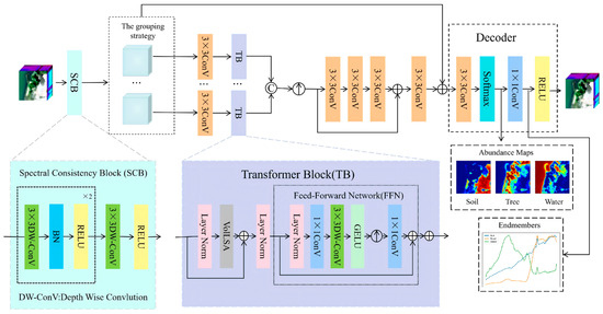
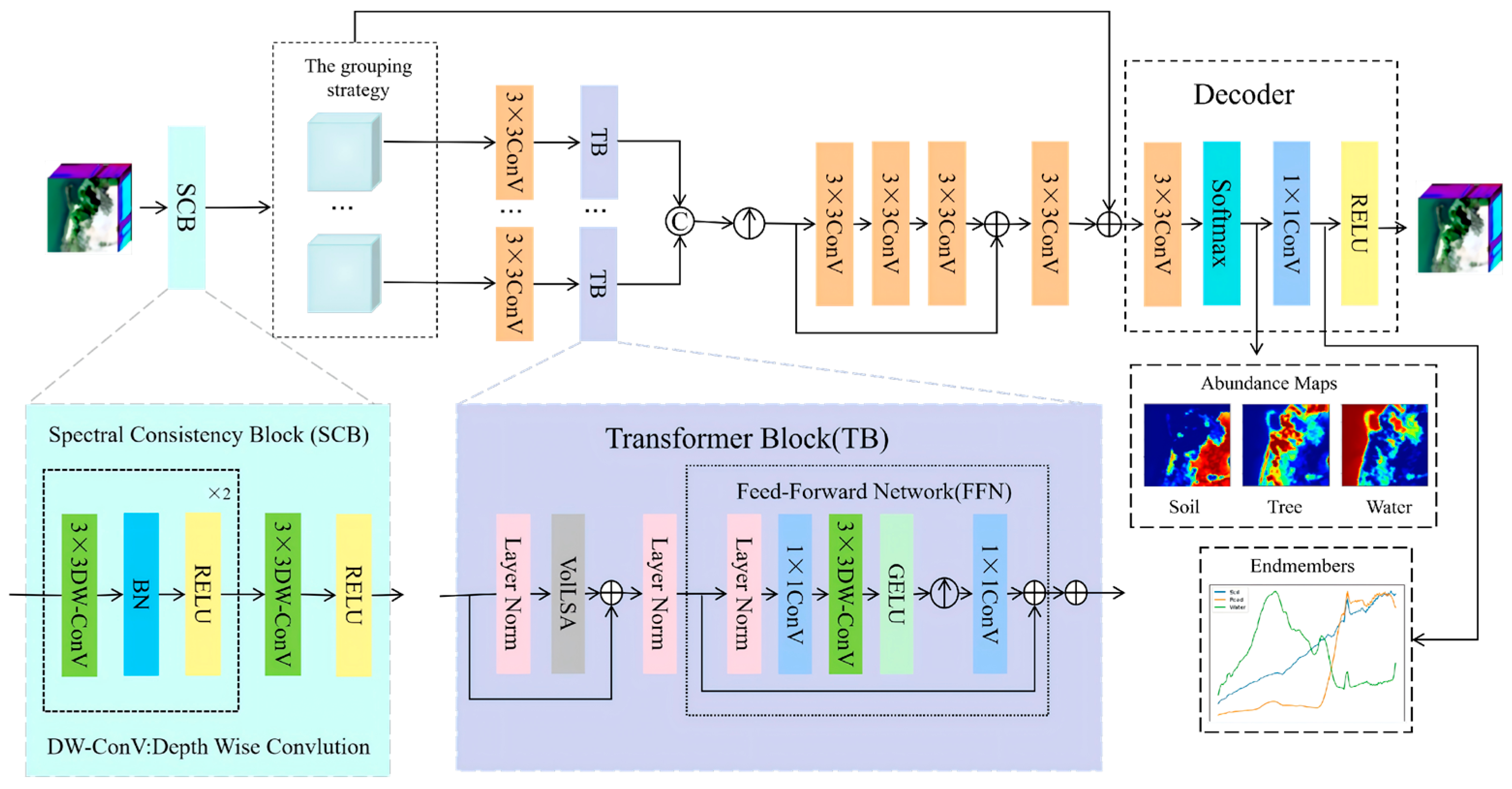
The proposed SCVolFormer (Spectral Consistency–guided Volumetric Linear Self-Attention Transformer) is introduced in this section. Its overall architecture is illustrated in Figure 1.

Figure 1. Overall architecture of SCVolFormer.

3.1. Spectral Consistency Block (SCB)

Conventional hyperspectral unmixing focuses on the spectral vector of an individual pixel $y_{i,j,:}$, which is modeled as a linear combination of r endmember signatures. From another perspective, if a single spectral band is considered, the corresponding band image $y_{:,:k}$ can also be regarded as a linear combination of r abundance maps:

$$y_{:,:,k}=E_{k,1}\times {\mathcal{A}}_{:,:,1}+\dots +E_{k,r}\times {\mathcal{A}}_{:,:,r}$$

(5)

where $k\in \left\{1,\dots ,L\right\}$. This formulation reveals that, although different spectral bands exhibit distinct spectral responses, they share the same underlying abundance distribution. In other words, each band image is generated from an identical set of abundance maps but with different endmember coefficients. Therefore, preserving spectral consistency across bands during feature extraction is crucial for accurate abundance estimation.

Motivated by this observation, we propose a Spectral Consistency Block (SCB). Unlike conventional convolutional modules, SCB employs depthwise convolutions to model each spectral channel independently. The initial feature extraction process is formulated as follows:

$$F_1={\varphi }_{DW}\left(Y\right)$$

(6)

where ${\varphi }_{DW}\left(\cdot \right)$ denotes a 3 × 3 depth–wise convolution. Since each convolution kernel operates exclusively on its corresponding spectral channel, no cross-band feature fusion is introduced at this stage. Consequently, the original spectral information is preserved to the greatest extent.

To further enhance feature representation, batch normalization and the ReLU activation function are subsequently applied, as follows:

$$F_2=\mathrm{Re}LU\left(BN\left(F_1\right)\right)$$

(7)

To exploit the local structural information within each spectral band while maintaining channel independence, another depthwise convolution is performed, as follows:

$$F_3={\varphi }_{DW}\left(\mathrm{Re}LU\left(BN\left(F_2\right)\right)\right)$$

(8)

Finally, the output of the Spectral Consistency Block is obtained as follows:

$$F_4={\varphi }_{DW}\left(\mathrm{Re}LU\left(F_3\right)\right)$$

(9)

3.2. Transformer Encoder

Although the features generated by the SCB preserve spectral consistency and effectively capture local spectral–spatial information, the locality of convolution operations limits their ability to model long-range dependencies across spectral bands and spatial regions. To address this limitation, a Transformer encoder equipped with the proposed Volumetric Linear Self-Attention (VolLSA) mechanism is introduced to further exploit global spectral–spatial correlations in hyperspectral data.

Considering the high computational cost of self-attention, a spectral grouping strategy is adopted to reduce the computational complexity while preserving local spectral continuity. Specifically, the output features of the SCB are evenly divided into m contiguous spectral groups, as follows:

$$F_4=\left\{G_1,G_2,\dots ,G_m\right\}$$

(10)

where $G_i\in {\mathbb{R}}^{H\times W\times L_g}$ denotes the i–th spectral group, and $L_g={\displaystyle \frac{L}{m}}$.

Each spectral group is then independently fed into a shared-weight Transformer encoder for feature extraction, as follows:

$$Z_i=T\left(G_i\right), i=1,\dots ,m$$

(11)

where $T\left(\cdot \right)$ denotes the Transformer encoder.

The parameter-sharing strategy is adopted based on the observation that different spectral groups exhibit similar statistical characteristics. Sharing encoder parameters therefore reduces the number of learnable parameters while improving the generalization capability of the model. After all spectral groups have been processed, the extracted features are concatenated along the spectral dimension to obtain the final feature representation, as follows:

$$Z=concat\left(Z_1,\dots ,Z_m\right)$$

(12)

3.2.1. Transformer Block

The shared-weight Transformer encoder consists of multiple Transformer Blocks (TBs). Given the input feature $X$, the $l$–th Transformer Block first applies Layer Normalization (LN) as follows:

$${\widehat{X}}^{l-1}=LN\left(X^{l-1}\right)$$

(13)

The normalized feature is then fed into the proposed Volumetric Linear Self-Attention (VolLSA) module, followed by a residual connection, as follows:

$$Y^l=VolLSA\left({\widehat{X}}^{l-1}\right)+X^{l-1}$$

(14)

The output is subsequently normalized again, as follows:

$${\widehat{Y}}^l=LN\left(Y^l\right)$$

(15)

and passed through a Feed-Forward Network (FFN) with another residual connection, as follows:

$$X^l=FFN\left({\widehat{Y}}^l\right)+Y^l$$

(16)

3.2.2. Volumetric Linear Self-Attention

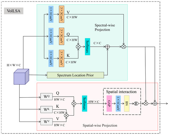
Existing self-attention mechanisms, including spatial self-attention and channel self-attention, establish long-range dependencies only on two-dimensional feature representations. Consequently, the intrinsic spectral–spatial correlations embedded in hyperspectral cubes cannot be fully exploited. To overcome this limitation, a Volumetric Linear Self-Attention (VolLSA) mechanism is introduced. Unlike conventional self-attention, VolLSA extends feature interactions from two-dimensional representations to three-dimensional hyperspectral cubes. Spectral and spatial dependencies are jointly modeled through two projected similarity matrices and their cross-covariance, thereby enabling efficient long-range spectral–spatial interactions.

As illustrated in Figure 2, a spectral projection matrix is first constructed by modeling the covariance among spectral channels, allowing global contextual information to be encoded along the spectral dimension. Given an input feature $X_{in}\in {\mathbb{R}}^{H\times W\times C}$, where W and H represent the width and height of the input, and C denotes the number of channels. By performing a 1 × 1 pointwise convolution WP followed by a 3 × 3 depthwise convolution WD, the query matrix $Q_{spe}\in {\mathbb{R}}^{C\times HW}$, key matrix $K_{spe}\in {\mathbb{R}}^{C\times HW}$, and value matrix $V_{spe}\in {\mathbb{R}}^{C\times HW}$ are generated from $X_{in}$. This projection formulation effectively enhances the representation capacity, which is formally defined as follows:

$$Q_{spe}=W_P^Q{W}_D^Q{X}_{in}, K_{spe}=W_P^K{W}_D^K{X}_{in}, V_{spe}=W_P^V{W}_D^V{X}_{in}$$

(17)

Figure 2. Architecture of the VolLSA.

Subsequently, a dot–product interaction operation is performed on $Q_{spe}$ and $K_{spe}$ to generate the spectral projection matrix $A_{spe}\in {\mathbb{R}}^{C\times C}$

$$A_{spe}=Soft\max \left({\displaystyle \frac{Q_{spe}\cdot K_{spe}}{\epsilon }}+B\right)$$

(18)

where $\epsilon$ is a learnable parameter that is utilized to weigh the dot product of $Q_{spe}$ and $K_{spe}$ before the Softmax function is applied. B denotes a learnable relative position encoding.

Traditional Transformers lack positional priors, whereas the retention mechanism in sequence modeling brings a temporal prior to language models. Inspired by the retention mechanism, a spectral positional prior is introduced, which is based on spectral wavelengths to describe spectral correlations. For HSIs with continuous, narrow-band spectra, the positional distance between spectra is related to the similarity among them. Bidirectional attenuation is exhibited by each spectrum, where attention is paid to both its preceding and succeeding spectra. Therefore, the temporal prior is extended into a bidirectional form to simulate the attenuation of bidirectional spectral correlations, as follows:

$$D_{nm}=\left\{\begin{array}{l}{\gamma }^{n-m}, n\ge m\hfill \\ {\gamma }^{m-n}, n<m\hfill \end{array}\right.$$

(19)

where $D_{nm}$ is a matrix that combines a causal mask and exponential spectral correlation decay based on relative distance. The original spectral projection matrix is combined with the spectral positional prior. The enhanced spectral projection matrix $A_{spe}$ can be expressed as follows:

$$A_{spe}=Soft\max \left({\displaystyle \frac{Q_{spe}\cdot K_{spe}}{\epsilon }}\odot D+B\right)$$

(20)

where ⊙ denotes element-wise multiplication.

To further improve the representation capability of the spectral projection matrix, information from different feature subspaces is projected into multiple attention heads. Specifically, the query matrix $Q_{spe}$, key matrix $K_{spe}$, and value matrix $V_{spe}$ are partitioned into g groups as follows:

$$Q_{spe}=\left[Q_{spe}^1,\dots ,Q_{spe}^q\right], K_{spe}=\left[K_{spe}^1,\dots ,K_{spe}^g\right], V_{spe}=\left[V_{spe}^1,\dots ,V_{spe}^g\right]$$

(21)

where each group has a dimension of ${\mathbb{R}}^{{\displaystyle \frac{C}{g}}\times HW}$. where all components belong to ${\mathbb{R}}^{{\displaystyle \frac{C}{g}}\times HW}$. Therefore, the spectral projection matrix $A_{spe}$ for the i–th head is given by the following:

$$A_{spe}^i=Soft\max \left({\displaystyle \frac{Q_{spe}^i\cdot K_{spe}^i}{\epsilon }}\odot D+B\right)$$

(22)

The latent output $Y_{spe}^i$ of the i–th head is defined as follows:

$$Y_{spe}^i=A_{spe}^i\cdot V_{spe}^i$$

(23)

Finally, the outputs of all attention heads are concatenated to produce the spectral feature representation

$$Y_{spe}=concat\left(Y_{spe}^1,\dots ,Y_{spe}^g\right)$$

(24)

The spatial projection branch models the interactions along the spatial dimension and generates a spatial attention map to capture long-range spatial dependencies. Given the input feature map $X_{in}$, it is projected into the query matrix $Q_{spa}\in {\mathbb{R}}^{HW\times C}$, key matrix $K_{spa}\in {\mathbb{R}}^{C\times HW}$, and value matrix as

$$Q_{spa}=W^Q X_{in}, K_{\mathit{spa}}{=W}^K X_{\mathit{in}}, V_{\mathit{spa}}{=W}^V X_{\mathit{in}}$$

(25)

where $W^Q$ and $W^K\in {\mathbb{R}}^{C\times C}$ are learnable projection matrices. The projected features are then divided into g attention heads, and a dot–product operation is then performed on $K_{spa}^i$ and $V_{spa}^i$ to generate the i–th spatial projection map $A_{spa}^i\in {\mathbb{R}}^{HW\times C}$ as follows:

$$A_{spa}^i=Soft\max \left(Q_{spa}^i\left({\displaystyle \frac{K_{spa}^i\cdot V_{spa}^i}{\sqrt{C}}}\right)+B\right)$$

(26)

Finally, the spatial attention features are fused with the spectral attention features to obtain the volumetric representation, as follows:

$$Y_{vol}=W_{out}\cdot \left(Y_{spe}\cdot A_{spa}+Y_{spe}\right)$$

(27)

where $W_{out}\in {\mathbb{R}}^{C\times C}$ is a learnable projection matrix.

3.2.3. Feed-Forward Network

The feed-forward network (FFN) consists of two 1 × 1 convolutional layers, one 3 × 3 depthwise convolutional layer, and a GELU activation function. The first 1 × 1 convolution projects and expands the channel features, while the depthwise convolution captures local spatial context. The second 1 × 1 convolution is then applied for feature fusion and channel restoration. The FFN output is formulated as

$$Y_{FFN}=Con{v}_{1\times 1}\left(GELU\left({\varphi }_{DW}\left(Con{v}_{1\times 1}\left(LN\left(Y_{vol}\right)\right)\right)\right)\right)$$

(28)

Subsequently, a residual connection is introduced to fuse the FFN output with the VolLSA features, yielding the output of the Transformer block, as follows:

$$X^l=Y_{vol}+Y_{FFN}$$

(29)

3.3. Decoder

The features output by the Transformer encoder is processed through three 3 × 3 convolutional layers with residual connections to generate the decoded feature $H$ as follows:

$$H_i={\varphi }_{DW}\left(H_{i-1}\right)+H_{i-1}, i=1,2,3$$

(30)

where $H_0$ denotes the output result of the Transformer encoder.

Although long-range dependencies can be effectively captured by the Transformer encoder, its primary focus is on high-level semantic information. In contrast, the shallow features extracted by the spectral consistency module (SCB) still retain abundant primitive spectral details and local structural information. Therefore, to further augment the feature representation capability, a residual connection strategy is adopted to fuse the output features of the SCB with the decoded features, yielding the feature map $F_{dec}$ as follows:

$$F_{dec}={\varphi }_{DW}\left(H_3\right)+F_4$$

(31)

where $F_4$ represents the feature output by the spectral consistency module (SCB).

Subsequently, the feature is passed through a 1 × 1 convolutional layer to map the channel number to the number of endmembers P, thereby generating the abundance map $A\in {\mathbb{R}}^{H\times W\times P}$ as follows:

$$A=Con{v}_{1\times 1}\left(H_{dec}\right)$$

(32)

To satisfy the physical constraints of hyperspectral unmixing, namely the abundance nonnegativity constraint (ANC) and the abundance sum-to-one constraint (ASC), a Softmax activation function is applied to normalize the abundance distribution of each pixel, as follows:

$${\widehat{A}}_{ij}={\displaystyle \frac{\exp \left(A_{ij}\right)}{{\displaystyle \sum _{P=1}^P\exp \left(A_{ip}\right)}}}$$

(33)

After abundance estimation, a linear reconstruction of the spectra is performed by the model using a trainable endmember matrix $\widehat{E}\in {\mathbb{R}}^{P\times C}$

$$\widehat{X}=\widehat{A}\widehat{E}$$

(34)

where $\widehat{X}$ denotes the hyperspectral image reconstructed by the model, and $\widehat{E}$ corresponds to the estimated set of endmember spectra.

3.4. Loss Function

The network is optimized through a composite objective that jointly balances reconstruction accuracy and spectral fidelity, as follows:

$$\mathcal{L}={\mathcal{L}}_{MSE}+\lambda {\mathcal{L}}_{SAD}$$

(35)

where $\lambda$ weights the relative contribution of magnitude-level reconstruction accuracy against spectral shape preservation.

The mean squared error (MSE) loss is employed to minimize the reconstruction error between the reconstructed spectra and the observed spectra, as follows:

$${\mathcal{L}}_{MSE}={\displaystyle \frac{1}{N}}{\displaystyle \sum _{i=1}^N\Vert X_i-{\widehat{X}}_i{\Vert }_2^2}$$

(36)

The spectral angle distance (SAD) loss is introduced to preserve spectral shape consistency, thereby improving the purity of the estimated endmembers, as follows:

$${\mathcal{L}}_{SAD}={\displaystyle \frac{1}{N}}{\displaystyle \sum _{i=1}^N\arccos \frac{X_i\cdot {\widehat{X}}_i}{\Vert X_i{\Vert }_2\Vert {\widehat{X}}_i{\Vert }_2}}$$

(37)

4. Experiments

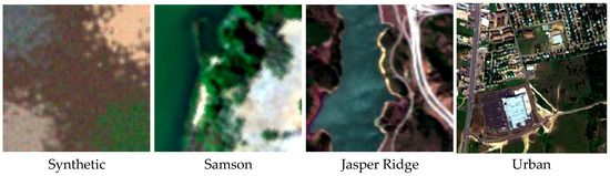
To comprehensively evaluate the effectiveness of the proposed method, experiments were conducted on one synthetic dataset and three real hyperspectral datasets, namely Samson, Jasper Ridge, and Urban. The corresponding RGB visualizations of the four datasets are presented in Figure 3.

Figure 3. True color images of experimental datasets.

The proposed method was compared with six representative hyperspectral unmixing approaches, including CyCU [26], MAT–Net [39], TCCU [38], CDCTA [40], DeepTrans [37], and MOGNMF [22], to demonstrate its superiority in hyperspectral unmixing.

4.1. Experimental Setup

4.1.1. Datasets

(1)

Synthetic Dataset [50]: This dataset comprises a 60 × 60 pixel image with L = 200 bands covering wavelengths from 0.4–1.4 μm. Five endmembers (Asphalt, Conifer, Concrete, Basalt, Limestone) are arranged with one serving as the background and the remaining four placed in the scene corners; abundances follow a Dirichlet distribution. For robustness evaluation under noise, controlled Gaussian noise is added under multiple SNR levels.

(2)

Samson Dataset [51]: This image contains 952 × 952 pixels with L = 156 bands (401–889 nm). A 95 × 95 crop starting at coordinate (252, 332) is used, covering the following three materials: Soil, Tree, and Water. All 156 bands are preserved, and reference abundance maps together with endmember signatures are supplied by the dataset providers.

(3)

Jasper Ridge Dataset [52]: Acquired over the Jasper Ridge Biological Preserve (California, USA), the full scene measures 512 × 614 pixels with L = 224 bands (380–2500 nm). Standard preprocessing removes water-absorption and low-SNR bands (1–3, 108–112, 154–166, 220–224), retaining 198 bands. A 100 × 100 sub-image starting at (105, 269) is analyzed, containing the following four endmembers: Tree, Soil, Water, and Road. Reference spectra are derived from manually delineated pure regions in the benchmark set.

(4)

Urban Dataset [53]: This HYDICE acquisition provides 307 × 307 pixels with L = 210 bands (400–2500 nm). After discarding water-absorption and low-quality channels, 162 bands remain. Four endmembers (Grass, Tree, Road, Roof) are present, with reference signatures and abundance maps sourced from the public benchmark.

4.1.2. Evaluation Metrics

We assess unmixing quality using three standard criteria. Reconstruction fidelity is measured by the average reconstruction error (RE) between original and reconstructed spectra. Abundance estimation accuracy is quantified via the root mean square error (RMSE) between predicted and reference abundance maps. Endmember quality is evaluated through the spectral angle distance (SAD) between extracted and reference endmember spectra. These metrics are defined as follows:

$$RE\left(X,\widehat{X}\right)={\displaystyle \frac{1}{N}}{\displaystyle \sum _{j=1}^{N}RE\left(x_j,{\widehat{x}}_j\right)}$$

(38)

$$RMSE\left({\widehat{a}}_j,a_j\right)=\sqrt{{\displaystyle \frac{1}{N}}{\displaystyle \sum _{j=1}^N{\left({\widehat{a}}_j-a_j\right)}^2}}$$

(39)

$$SAD\left(e_m,{\widehat{e}}_m\right)=\arccos {\displaystyle \frac{e_m\cdot {\widehat{e}}_m}{\Vert e_m{\Vert }_2\Vert {\widehat{e}}_m{\Vert }_2}}$$

(40)

where ${\widehat{x}}_j,{\widehat{a}}_j,{\widehat{e}}_m$ denote the reconstructed hyperspectral image, the estimated abundance map, and the estimated endmember matrix, respectively, while $x_j,a_j,e_m$ represent the corresponding ground–truth hyperspectral image, abundance map, and endmember matrix.

4.1.3. Experimental Settings and Computational Complexity Analysis

All experiments were conducted on a workstation equipped with an Intel(R) Core(TM) i5–10210U CPU, an NVIDIA GeForce MX250 GPU, and Python 3.10. The hyperparameter settings used for different datasets are summarized in Table 1. In Table 1, n_subs represents the number of spectral bands in each spectral group during spectral partitioning. Different values are adopted according to the spectral dimensionality of each dataset to balance spectral representation capability and computational efficiency.

Table 1. Network hyperparameter settings.

Parameters	Synthetic	Samson	Jasper Ridge	Urban
Learning rate	3 × 10−3	7 × 10−3	1 × 10−4	1 × 10−3
β	3 × 103	9 × 103	4 × 102	1 × 102
γ	3 × 10−2	8 × 10−3	4 × 10−2	1 × 10−2
Epoch	600	500	200	100
Weight decay	1 × 10−5	3 × 10−6	4 × 10−5	4 × 10−5
Dim	100	64	128	32
n_subs	40	39	33	27

To evaluate the computational efficiency of SCVolFormer, the number of parameters, floating-point operations (FLOPs), and GPU memory consumption were analyzed on four hyperspectral datasets. All complexity measurements were obtained using the final model configurations listed in Table 1 with a unified embedding dimension of 64. The results are summarized in Table 2. As shown in Table 2, SCVolFormer maintains a compact model size across different datasets, with the number of parameters ranging from 1.525 M to 1.562 M. The slight variation in parameter numbers mainly comes from the different spectral dimensions and the corresponding input/output projection layers. Since the embedding dimension is fixed, the proposed model avoids significant parameter growth when processing hyperspectral images with different spectral characteristics. The computational cost is mainly influenced by the spatial resolution of the input hyperspectral images. The FLOPs increase from 21.51 G on the Synthetic dataset to 589.45 G on the Urban dataset, which is mainly attributed to the increasing number of spatial pixels rather than the growth of model parameters. For example, although the Urban dataset contains a much larger spatial size (307 × 307 pixels), its parameter number remains comparable to other datasets. This demonstrates that SCVolFormer can effectively process large-scale hyperspectral images without introducing excessive parameter overhead. Furthermore, the GPU memory consumption shows a similar trend with spatial resolution. The memory requirement increases from 125.90 MB for the Synthetic dataset to 940.47 MB for the Urban dataset, mainly due to the larger intermediate feature maps generated during spectral–spatial feature extraction. These results verify that the proposed VolLSA-based architecture achieves efficient computational performance while maintaining effective spectral–spatial representation capability.

Table 2. Computational complexity of SCVolFormer on different datasets.

Datasets	Spatial Size (H × W)	Bands(L)	Parameters (M)	FLOPs (G)	GPU memory (MB)
Synthetic	60 × 60	200	1.562	21.51	125.90
Samson	95 × 95	156	1.535	38.76	168.96
Jasper Ridge	100 × 100	198	1.554	66.74	188.90
Urban	307 × 307	162	1.525	589.45	940.47

4.1.4. Computational Comparison of Different Attention Mechanisms

To further verify the computational advantage of the proposed VolLSA, different attention variants are compared in terms of parameters, FLOPs, and GPU memory consumption on the Synthetic dataset. As shown in Table 3, Channel Self-Attention (CSA) and spatial attention modules, including Spatial Self-Attention (SSA) and Linear Self-Attention (LSA), individually introduce relatively limited computational costs, while combining spectral and spatial attention results in increased complexity. Specifically, integrating CSA and SSA results in a computational cost of 22.01 G FLOPs and a GPU memory consumption of 944.22 MB. By replacing the SSA with LSA, the proposed VolLSA reduces the GPU memory consumption to 864.60 MB while maintaining the same FLOPs (21.51 G), demonstrating the efficiency of linear attention in spatial dependency modeling. Furthermore, the introduced spectral location prior does not introduce additional parameters or computational overhead, as VolLSA and VolLSA without prior maintain identical FLOPs and parameter numbers.

Table 3. Computational comparison of different attention mechanisms on the Synthetic dataset.

Attention	Spatial Attention	Spectral Attention	Parameters (M)	FLOPs (G)	GPU memory (MB)
CSA	–	CSA	0.92	12.62	721.68
SSA	SSA	–	0.91	12.84	687.51
LSA	LSA	–	0.90	12.33	592.34
CSA + SSA	SSA	CSA	1.37	22.01	944.22
VolLSA w/o prior	LSA	CSA	1.56	21.51	866.38
VolLSA	LSA	CSA	1.56	21.51	864.63

4.1.5. Noise Robustness Analysis

To evaluate the robustness of SCVolFormer against noise contamination, experiments were conducted on the Synthetic dataset by adding Gaussian noise with different signal-to-noise ratios (SNRs). The SNR levels were set to 30 dB, 20 dB, and 10 dB, while the clean data were used as the reference. The reconstruction error (RE), abundance RMSE, and spectral angle distance (SAD) are reported in Table 4. As shown in Table 4, SCVolFormer maintains stable performance under moderate noise levels. When the SNR decreases from the clean condition to 30 dB and 20 dB, the RE increases slightly from 0.003540 to 0.011094, while the SAD remains within a relatively small range. This indicates that the proposed spectral consistency constraint and VolLSA module can effectively suppress moderate noise interference by exploiting spectral–spatial correlations. Under severe noise conditions (10 dB), the performance degradation becomes more significant, with the RMSE increasing to 0.120179 and the SAD increasing to 0.08918. This degradation mainly results from strong spectral distortion, which affects the discrimination of similar materials and introduces uncertainty into abundance estimation. Nevertheless, SCVolFormer still preserves reasonable reconstruction capability, demonstrating its robustness against noisy hyperspectral observations.

Table 4. Performance of SCVolFormer under different Gaussian noise levels on the Synthetic dataset.

SNR (dB)	RE	RMSE	SAD
clean	0.003540	0.013867	0.005116
30	0.005052	0.022021	0.009009
20	0.011094	0.027844	0.015358
10	0.033076	0.120179	0.089182

4.1.6. Spectral Variability Robustness Analysis

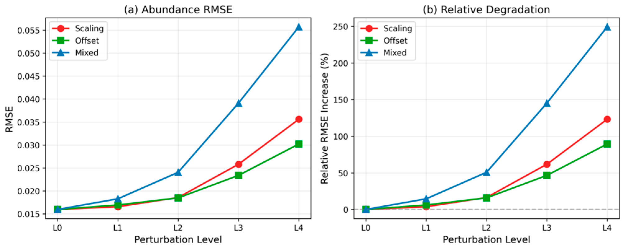
To evaluate the robustness of SCVolFormer against spectral variability, endmember perturbation experiments were conducted on the Synthetic dataset. Three perturbation types were considered, including multiplicative perturbation (Scaling), additive perturbation (Offset), and mixed perturbation (Mixed), which simulate spectral variations caused by illumination changes, sensor offsets, and combined effects in practical scenarios. Five perturbation levels were designed, ranging from Level 0 (clean data) to Level 4 (severe perturbation). The model was trained only on the original dataset and evaluated under different perturbation conditions.

Table 5 summarizes the performance variation under different perturbation settings. As the perturbation intensity increases, the abundance estimation error gradually increases for all perturbation types, while the degradation remains gradual and the model does not exhibit catastrophic failure. Among the three perturbations, Offset produces the smallest degradation, with an RMSE increase of 89.4% from Level 0 to Level 4. Scaling causes a larger performance decrease with an RMSE increase of 123.2%, while Mixed perturbation introduces both spectral scaling and offset effects, resulting in the largest degradation (249.3%). Nevertheless, even under the most severe Mixed Level 4 condition, the RMSE remains at 0.056, demonstrating the robustness of SCVolFormer under strong spectral variations.

Table 5. Robustness analysis under different spectral perturbations on the Synthetic dataset. Note: Each entry is reported as RMSE/SAD, where RMSE represents the abundance estimation error and SAD represents the spectral angle distance of extracted endmembers. L0–L4 denote increasing perturbation levels, from clean data to severe spectral variability.

Perturbation	L0 (Clean)	L1 (Mild)	L2 (Moderate)	L3 (Strong)	L4 (Severe)	ΔRMSE(%)
Scaling	0.0159/0.0062	0.0165/0.0207	0.0186/0.0481	0.0258/0.0948	0.0356/0.1418	+123.2%
Offset	0.0159/0.0062	0.0169/0.0142	0.0185/0.0313	0.0234/0.0609	0.0302/0.0901	+89.4%
Mixed	0.0159/0.0062	0.0183/0.0241	0.0241/0.0568	0.0391/0.1121	0.0557/0.1668	+249.3%

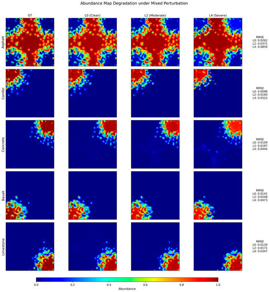
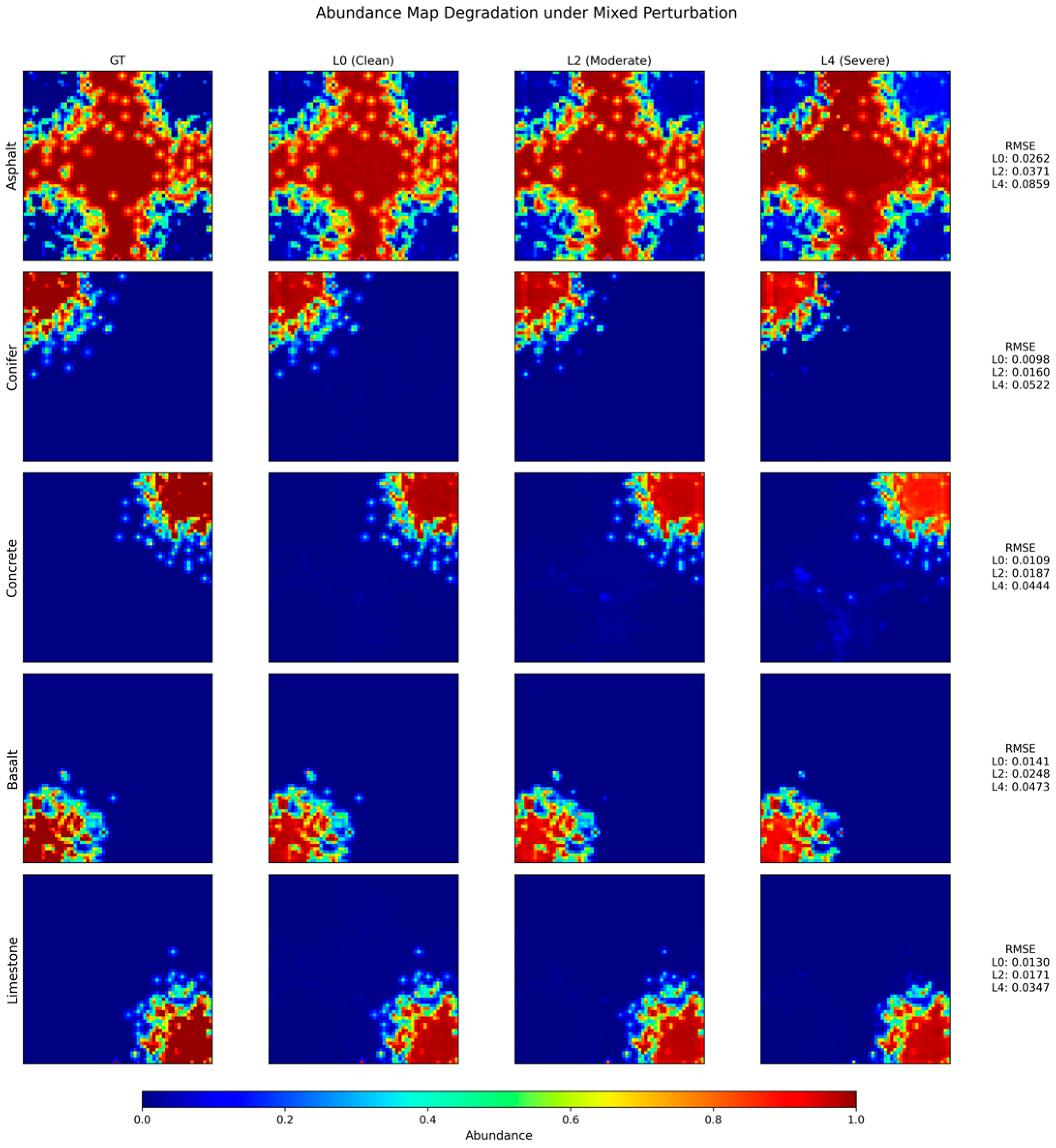
Figure 4 illustrates the abundance map variations of five endmembers under Mixed perturbation. For visualization clarity, only three representative levels, including Level 0 (clean), Level 2 (moderate), and Level 4 (severe), are presented. With increasing perturbation intensity, some spatial details become less distinct and boundaries become slightly blurred. However, the overall abundance distributions remain consistent, which agrees with the quantitative evaluation.

Figure 4. Visualization of Abundance Map Degradation under Mixed Endmember Spectral Perturbations.

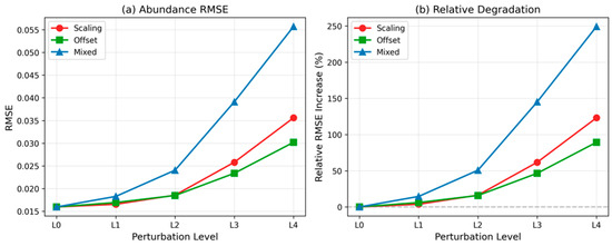
Figure 5a illustrates the variation in abundance estimation RMSE under different perturbation types, where L0–L4 represent five perturbation levels from clean to severe conditions. The RMSE gradually increases with the perturbation intensity for all three perturbation types, indicating that spectral variability inevitably affects abundance estimation. Among them, Offset perturbation causes the slowest error increase, while Mixed perturbation introduces the most significant degradation due to the combined effects of spectral scaling and offset. Figure 5b presents the relative RMSE increase with respect to the clean condition, providing a quantitative evaluation of the model sensitivity to spectral variability. The results show that SCVolFormer maintains a smooth degradation trend under different perturbation scenarios without catastrophic failure. At Level 4, the RMSE increases for Scaling, Offset, and Mixed perturbations are 123.2%, 89.4%, and 249.3%, respectively. Although Mixed perturbation causes the largest degradation, the absolute RMSE remains low (0.0557), demonstrating the robustness of SCVolFormer against spectral variations.

Figure 5. Quantitative Evaluation of Robustness under Different Spectral Perturbation Levels. (a) Abundance RMSE under Different Perturbation Levels. (b) Relative Performance Degradation with Increasing Perturbation Intensity.

Figure 6 further compares the reference, perturbed, and recovered endmember spectra under Level 3 Mixed perturbation. Although the perturbed spectra show noticeable deviations from the reference spectra, the recovered endmembers preserve similar spectral trends and characteristic variations, indicating the capability of SCVolFormer to maintain reliable spectral estimation under variable conditions.

Figure 6. Spectral Recovery of Estimated Endmembers under Mixed Perturbations.

4.2. Unmixing Performance Comparisons and Analysis

4.2.1. Experiment Results and Analysis

(1)

Synthetic Dataset: Quantitative results reported in Table 6 and Table 7 confirm that SCVolFormer attains the strongest overall performance across both metrics. For abundance estimation, the mean RMSE reaches 0.013867; for endmember extraction, the mean SAD drops to 0.005116—a clear margin below all competing approaches.

Table 6. RMSE results of abundance estimation on the Synthetic dataset. Best results are shown in bold.

	CyCU	MAT–Net	TCCU	CDCTA	DeepTrans	MOGNMF	Proposed
Asphalt	0.212267	0.023118	0.178095	0.124731	0.077719	0.301419	0.022752
Conifer	0.075195	0.010474	0.045452	0.044407	0.02266	0.2117	0.010319
Concrete	0.202546	0.014359	0.086241	0.063809	0.039133	0.164475	0.009841
Basalt	0.06019	0.008740	0.02925	0.115353	0.012115	0.15707	0.009776
Limestone	0.078678	0.012677	0.051927	0.099183	0.025527	0.216733	0.012040
Mean RMSE	0.12578	0.013874	0.094629	0.094599	0.042151	0.216502	0.013867

Table 7. SAD results of endmember estimation on the Synthetic dataset. Best results are shown in bold.

	CyCU	MAT–Net	TCCU	CDCTA	DeepTrans	MOGNMF	Proposed
Asphalt	0.038516	0.009897	0.106838	0.012836	0.013716	0.097935	0.005437
Conifer	0.02366	0.005869	0.002966	0.008621	0.014773	0.003665	0.004186
Concrete	0.037079	0.006740	0.015978	0.016285	0.020274	0.005939	0.007873
Basalt	0.02762	0.004523	0.014222	0.018939	0.009475	0.007611	0.005236
Limestone	0.023848	0.006469	0.004244	0.005796	0.005181	0.002206	0.002847
Mean SAD	0.03015	0.006699	0.028849	0.012495	0.012684	0.023471	0.005116

(2)

Samson Dataset: Table 8 and Table 9 confirm that SCVolFormer attains the strongest overall performance across both metrics. For abundance estimation, the mean RMSE reaches 0.013867; for endmember extraction, the mean SAD drops to 0.005116—a clear margin below all competing approaches.

Table 8. RMSE results of abundance estimation on the Samson dataset. Best results are shown in bold.

	CyCU	MAT–Net	TCCU	CDCTA	DeepTrans	MOGNMF	Proposed
Soil	0.094999	0.131851	0.070389	0.116132	0.066872	0.133577	0.062923
Tree	0.091981	0.124031	0.089077	0.061404	0.068753	0.134266	0.057437
Water	0.114073	0.209123	0.060503	0.11185	0.078736	0.197047	0.041293
Mean RMSE	0.10035	0.155002	0.074274	0.099611	0.071643	0.157795	0.054661

Table 9. SAD results of endmember estimation on the Samson dataset. Best results are shown in bold.

	CyCU	MAT–Net	TCCU	CDCTA	DeepTrans	MOGNMF	Proposed
Soil	0.025898	0.017577	0.018725	0.025516	0.008788	0.059	0.023408
Tree	0.09576	0.094066	0.087918	0.076929	0.055524	0.079612	0.054520
Water	0.155353	0.052464	0.128033	0.046988	0.088204	0.11255	0.062747
Mean SAD	0.09234	0.054702	0.078225	0.049811	0.050838	0.08372	0.046892

(3)

Jasper Ridge Dataset: Table 10 and Table 11 report performance on this scene. While several competing methods achieve isolated best scores on individual endmembers, SCVolFormer records the lowest mean RMSE (0.078729) and mean SAD (0.069818). The RMSE improvement over the runner-up (DeepTrans) is 0.008263, while SAD surpasses MAT–Net by 0.002472, highlighting consistent gains particularly in tree abundance estimation.

Table 10. RMSE results of abundance estimation on the Jasper Ridge dataset. Best results are shown in bold.

	CyCU	MAT–Net	TCCU	CDCTA	DeepTrans	MOGNMF	Proposed
Tree	0.146411	0.092519	0.141819	0.207404	0.098407	0.13636	0.072636
Water	0.239143	0.092593	0.110187	0.106293	0.106593	0.036376	0.059761
Soil	0.142267	0.092802	0.140365	0.279079	0.075827	0.155773	0.101041
Road	0.288608	0.079496	0.115388	0.244931	0.058947	0.105436	0.075741
Mean RMSE	0.20411	0.089352	0.127740	0.219198	0.086992	0.117579	0.078729

Table 11. SAD results of endmember estimation on the Jasper Ridge dataset. Best results are shown in bold.

	CyCU	MAT–Net	TCCU	CDCTA	DeepTrans	MOGNMF	Proposed
Tree	0.090107	0.090409	0.145768	0.044338	0.101541	0.140461	0.084983
Water	0.090061	0.082193	0.121577	0.149058	0.157014	0.114126	0.11333
Soil	0.116542	0.062417	0.109088	0.209606	0.032076	0.082422	0.0458881
Road	0.148142	0.054140	0.048636	0.122741	0.023632	0.043674	0.0350731
Mean SAD	0.11121	0.072290	0.106267	0.131436	0.078566	0.095171	0.069818

(4)

Urban Dataset: Table 12 and Table 13 present results for this challenging urban scene, which features numerous spectral bands and heterogeneous land cover. SCVolFormer continues to exhibit strong generalization, as follows: its mean RMSE of 0.140484 edges out TCCU (0.146767), and its mean SAD of 0.1184 marks an additional improvement over TCCU, underscoring the method’s robustness on complex real-world HSI distributions.

Table 12. RMSE results of abundance estimation on the Urban dataset. Best results are shown in bold.

	CyCU	MAT–Net	TCCU	CDCTA	DeepTrans	MOGNMF	Proposed
Road	0.288477	0.159642	0.120898	0.30526	0.159007	0.176714	0.163849
Grass	0.162322	0.159642	0.194421	0.286448	0.237438	0.153561	0.19235
Tree	0.159856	0.150966	0.150766	0.23569	0.122583	0.139622	0.09408
Roof	0.292326	0.124297	0.104956	0.407815	0.111997	0.146471	0.079039
Mean RMSE	0.22575	0.146911	0.146767	0.315079	0.16525	0.154723	0.140484

Table 13. SAD results of endmember estimation on the Urban dataset. Best results are shown in bold.

	CyCU	MAT–Net	TCCU	CDCTA	DeepTrans	MOGNMF	Proposed
Road	0.144804	0.252696	0.159585	0.16452	0.282567	0.42741	0.2096
Grass	0.099159	0.11782	0.143961	0.285562	0.188515	0.159111	0.092126
Tree	0.275517	0.040068	0.112716	0.074515	0.135066	0.112076	0.083379
Roof	0.104389	0.160358	0.081997	0.094725	0.1217	0.140208	0.088496
Mean SAD	0.15597	0.142736	0.124565	0.15483	0.181962	0.209701	0.1184

4.2.2. Visual Analysis

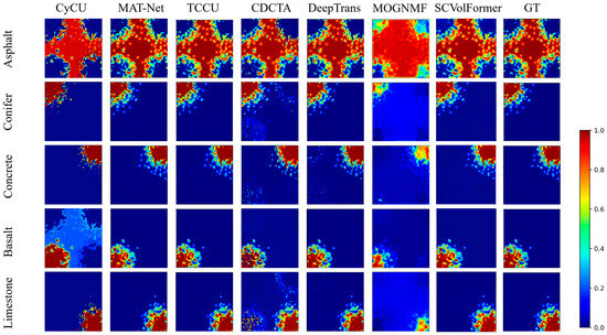
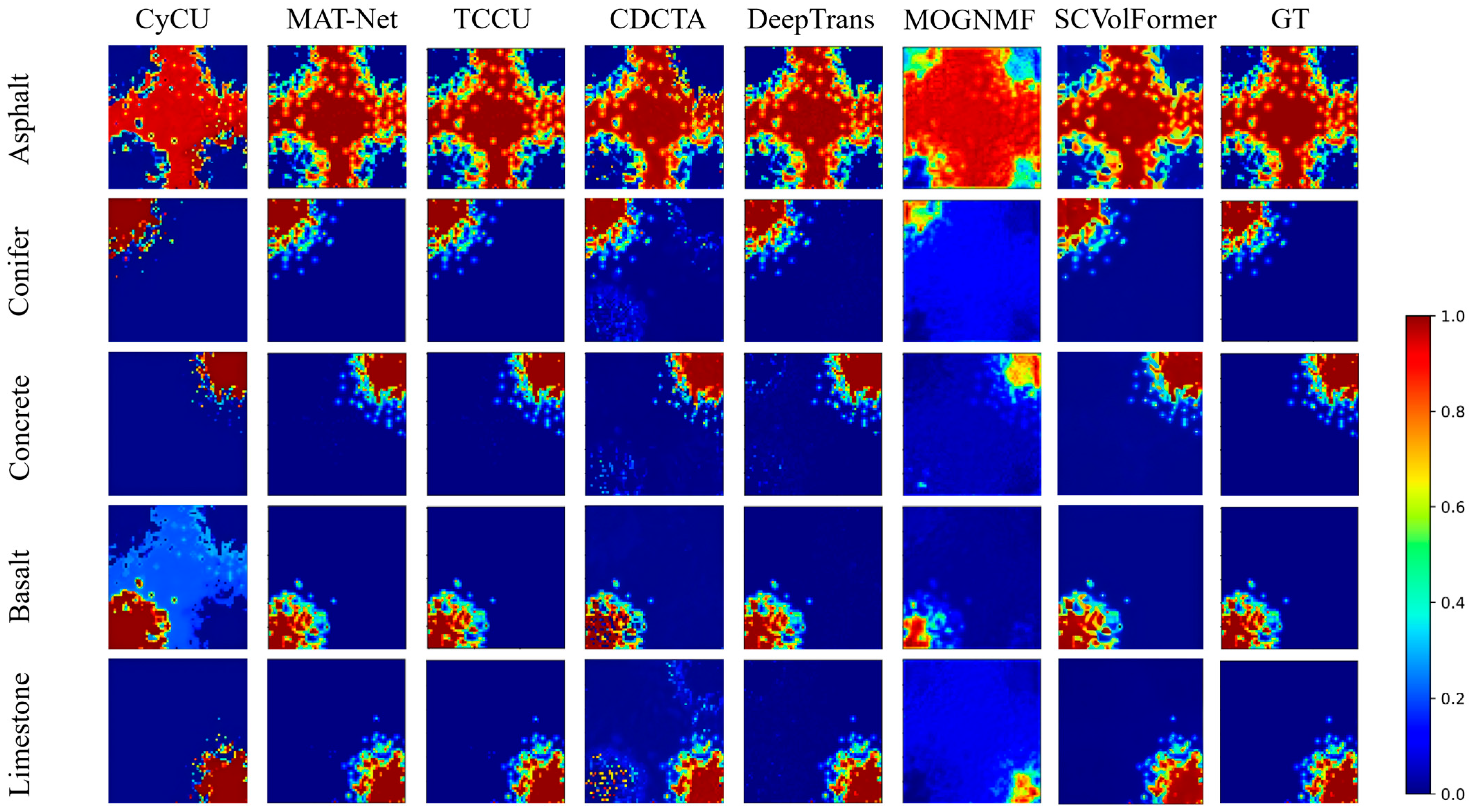
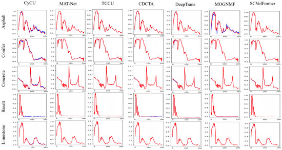
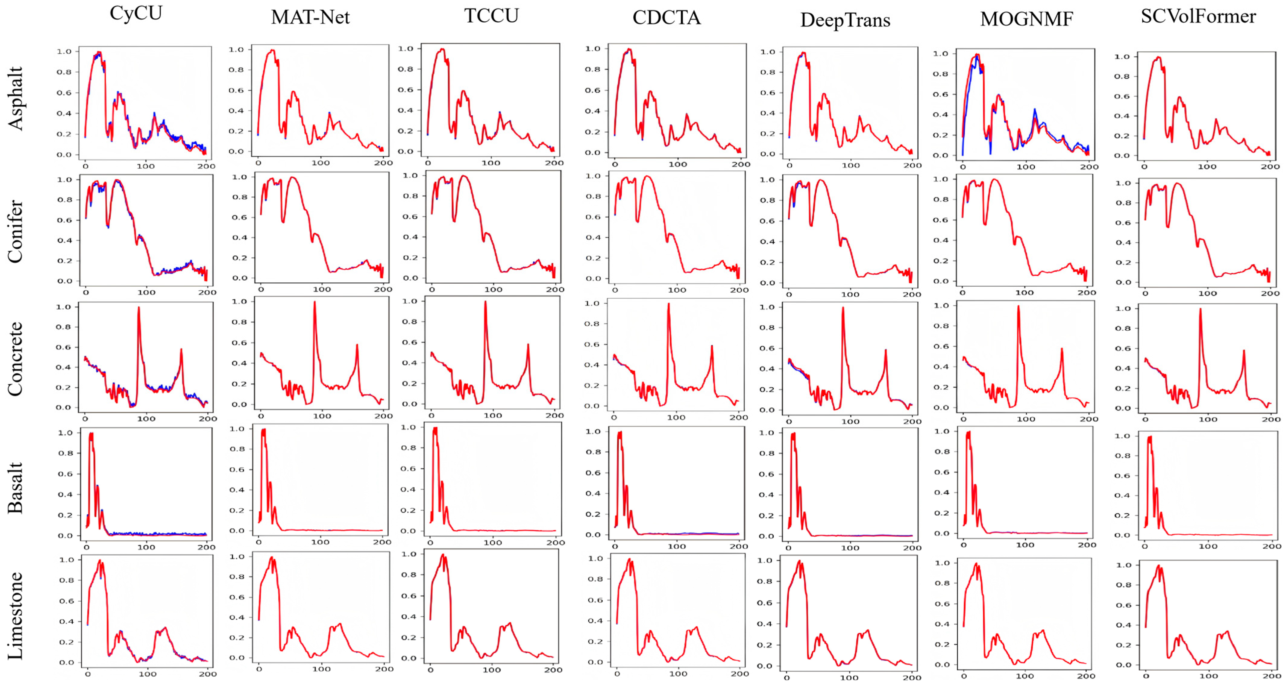
Figure 7 and Figure 8 provide a qualitative comparison of abundance maps and endmember spectra produced by all methods on the Synthetic dataset. The abundance maps reveal clear differences in how well each method reconstructs target endmember regions and suppresses spurious responses in non-target areas.

Figure 7. Abundance maps estimated by different unmixing methods on the Synthetic dataset. The GT column shows the GT abundance maps.

Figure 8. Reference signatures (red) and estimated endmember signatures (blue) by different unmixing methods on the Synthetic dataset.

The traditional method MOGNMF is more susceptible to noise, resulting in obvious abundance responses in non-target endmember regions and blurred boundaries of the target endmembers, leading to a considerable discrepancy from the ground truth (GT). In comparison, CyCU is capable of recovering the major distribution of each endmember, although response spreading can still be observed in several endmember regions. CDCTA produces abundance maps that are generally consistent with the GT; however, deviations remain around endmember boundaries and in regions occupied by small targets. TCCU, MAT–Net, and DeepTrans provide relatively stable abundance estimation results, but sparse responses are still visible around several endmember regions. In contrast, the abundance maps generated by SCVolFormer show the highest visual consistency with the GT. The proposed method accurately preserves the spatial distribution of the target endmembers while effectively suppressing responses in non-target endmember regions, resulting in clearer boundaries between adjacent endmembers.

Figure 8 also presents the endmember spectra extracted by different methods. Most deep learning–based methods are able to capture the overall spectral trends of the endmembers, although noticeable discrepancies remain in several spectral regions. Among the compared methods, MOGNMF exhibits the largest deviation for the Asphalt endmember. CyCU also shows slight discrepancies for the Asphalt, Conifer, Concrete, and Basalt endmembers. By contrast, the endmember spectra estimated by SCVolFormer achieve the closest agreement with the reference spectra for all five endmembers.

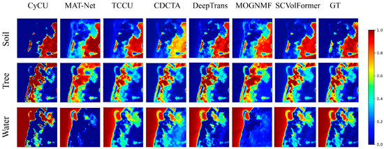
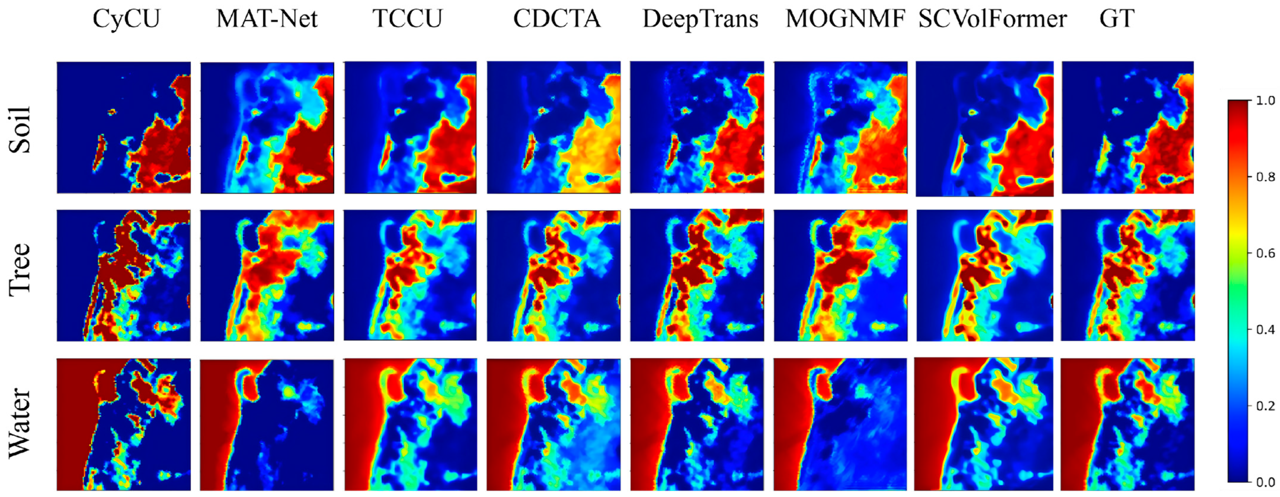
To further evaluate the unmixing performance of the proposed method in real-world scenarios, the abundance maps estimated on the Samson dataset are presented in Figure 9. This scene contains a large number of mixed pixels at material boundaries (e.g., the yellow-green transition regions), posing a challenge for accurate abundance estimation in transition areas.

Figure 9. Abundance maps estimated by different unmixing methods on the Samson dataset. The GT column shows the GT abundance maps.

As shown in Figure 9, CyCU exhibits obvious abundance overestimation. Many mixed pixels in the transition regions (yellow-green in the ground truth) are estimated as high-abundance pure pixels (red), resulting in excessively large high-response regions for the target endmembers and deviating from the physical mixing characteristics. In contrast, MAT–Net and MOGNMF tend to underestimate abundance values. Regions with moderate abundances (green in the ground truth) are directly estimated as near-zero abundances (dark blue), leading to the loss of spatial details and fine-scale abundance variations. TCCU, CDCTA, and DeepTrans are able to recover the overall distribution of the endmembers. However, background responses and boundary spreading can still be observed in the transition regions between the soil and water endmembers.

In comparison, the abundance maps produced by SCVolFormer are the closest to the ground truth. The proposed method not only accurately recovers the spatial distributions of different endmembers but also preserves the continuous abundance variations in mixed regions. In particular, the transition regions with low and moderate abundances between the water and soil endmembers agree well with the ground truth. Clearer boundaries are preserved, while low responses are maintained in non-target endmember regions.

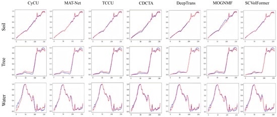
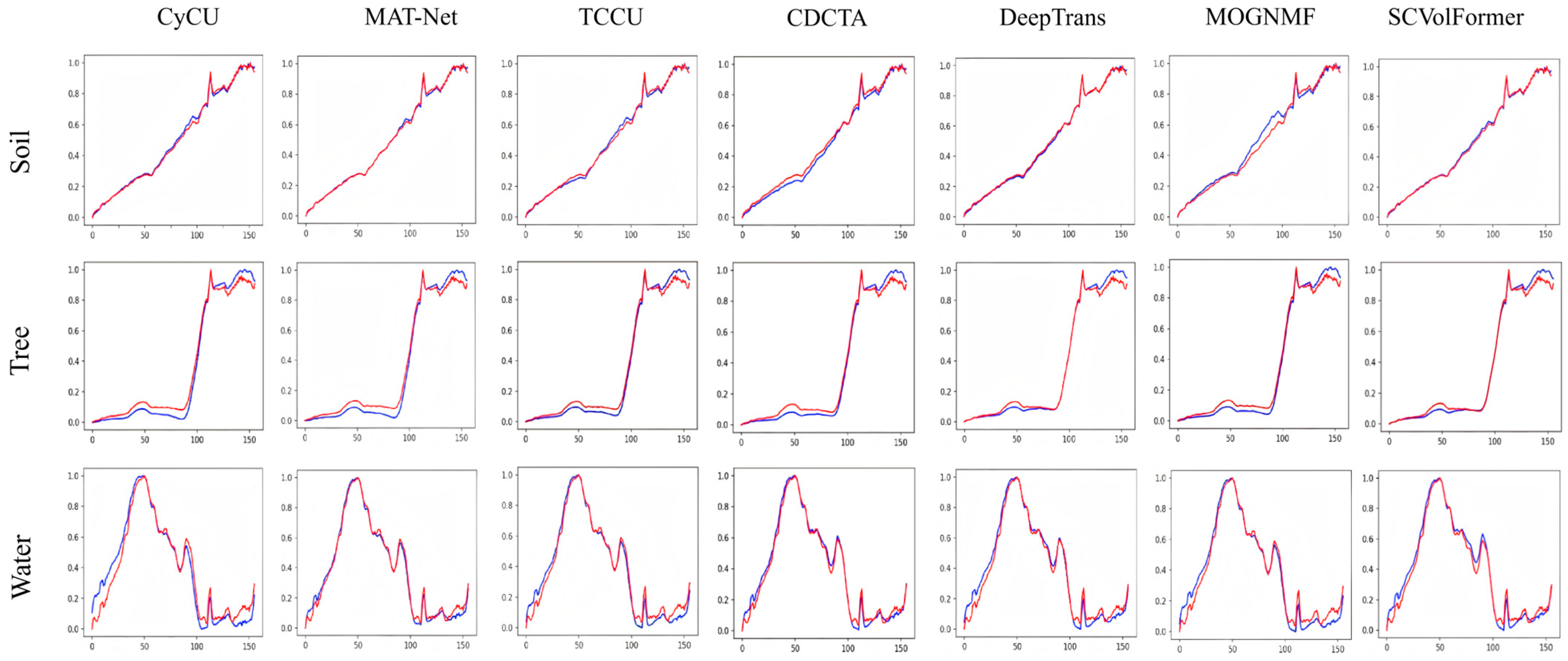
Figure 10 also presents the endmember spectra extracted by different methods. Most deep learning methods are able to recover the overall spectral trends of the endmembers, although noticeable deviations remain in several local spectral bands. CyCU and MOGNMF show relatively large fitting errors for the water endmember. MAT–Net, TCCU, CDCTA, and DeepTrans capture the overall spectral shapes reasonably well, but discrepancies are still observed around local peaks and valleys. In contrast, the endmember spectra estimated by SCVolFormer show high agreement with the reference spectra for all three endmembers (soil, tree, and water). Accurate spectral fitting is maintained even in wavelength ranges with significant spectral variations.

Figure 10. Reference signatures (red) and estimated endmember signatures (blue) by different unmixing methods on the Samson dataset.

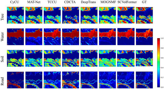
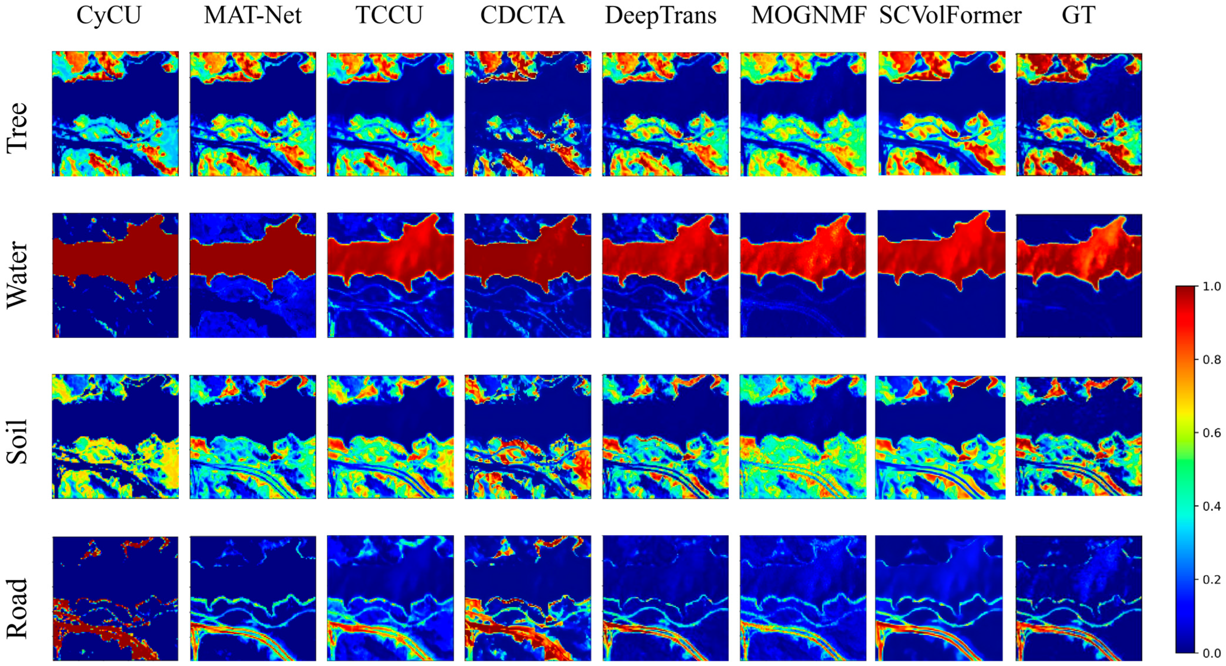
To further evaluate the unmixing performance of different methods in complex natural scenes, the abundance maps and extracted endmember spectra on the Jasper Ridge dataset are shown in Figure 11. Noticeable differences can be observed among the compared methods in recovering complex land-cover structures and mixed regions.

Figure 11. Abundance maps estimated by different unmixing methods on the Jasper Ridge dataset. The GT column shows the GT abundance maps.

For the road endmember, which is characterized by a narrow and elongated spatial distribution, CyCU estimates the road as a much larger high-abundance region, resulting in a significantly wider distribution than the ground truth. MAT–Net, TCCU, and DeepTrans are able to recover the overall road structure, but abundance spreading can still be observed along the local boundaries. The abundance maps generated by MOGNMF are relatively smooth, causing part of the road details to be lost. For the water endmember, MAT–Net, DeepTrans, and MOGNMF still produce noticeable responses in non-target regions, whereas SCVolFormer effectively suppresses these responses and produces clearer boundaries between water and the surrounding areas. For the tree and soil endmembers, the major spatial distributions are recovered by all deep-learning methods. However, blurred boundaries or scattered responses are still observed in the transition regions between adjacent endmembers. In comparison, SCVolFormer preserves smoother abundance variations in mixed regions, producing results that are visually closer to the ground truth.

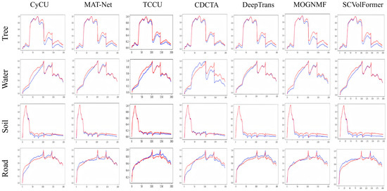
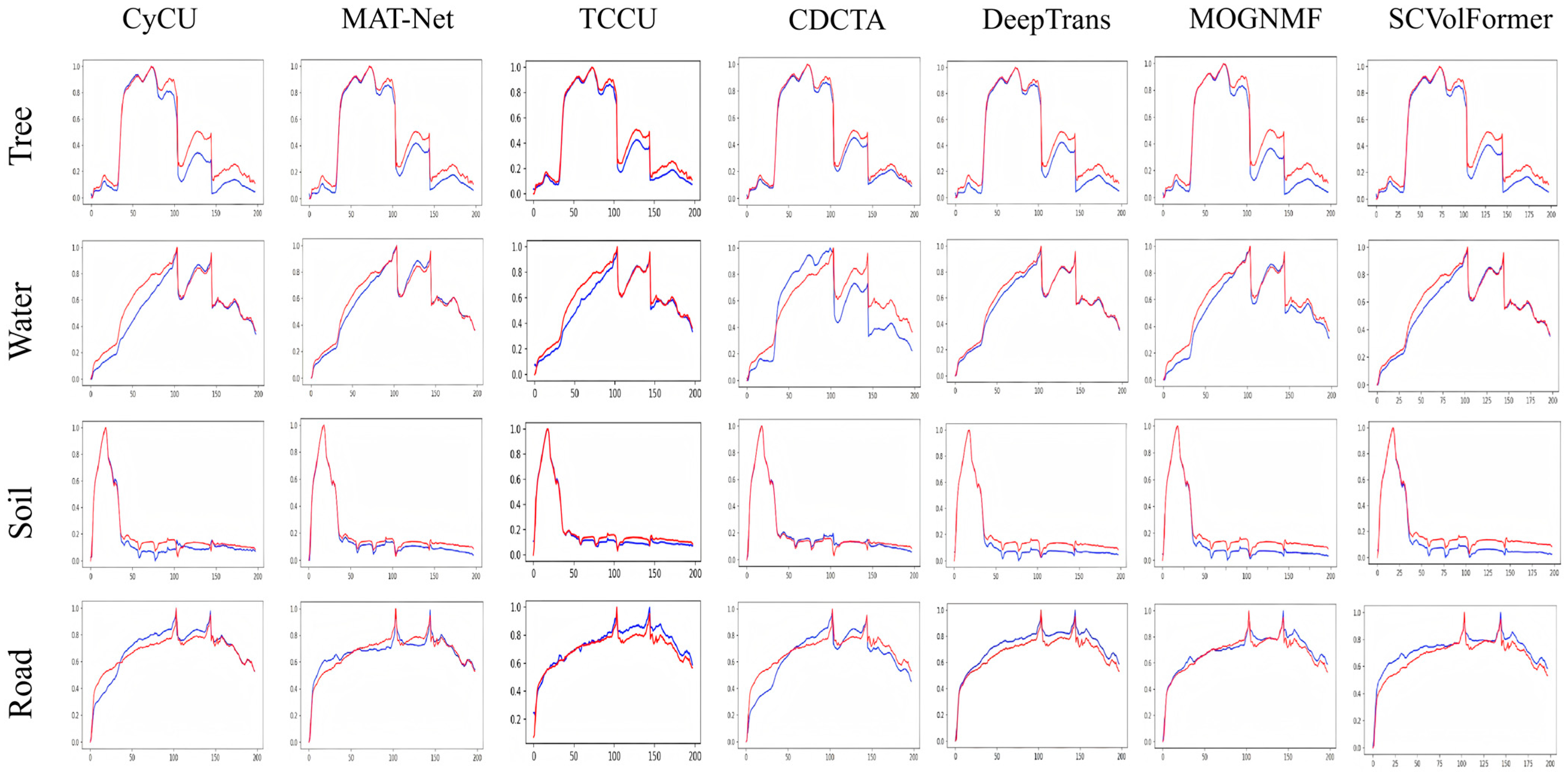
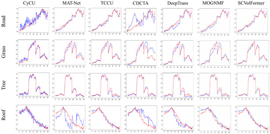
Figure 12 also presents the endmember spectra extracted by different methods. It can be observed that all methods are able to capture the overall spectral trends of the endmembers, while noticeable discrepancies remain in several wavelength ranges. Among the compared methods, CyCU and CDCTA exhibit relatively large fitting errors for the water and road endmembers. Although MAT–Net, TCCU, MOGNMF, and DeepTrans generally follow the overall spectral shapes, deviations can still be observed around several spectral peaks and valleys. In contrast, the Tree, water, soil, and road endmember spectra extracted by SCVolFormer show a higher degree of agreement with the reference spectra and provide more accurate fitting over the major characteristic wavelength ranges.

Figure 12. Reference signatures (red) and estimated endmember signatures (blue) by different unmixing methods on the Jasper Ridge dataset.

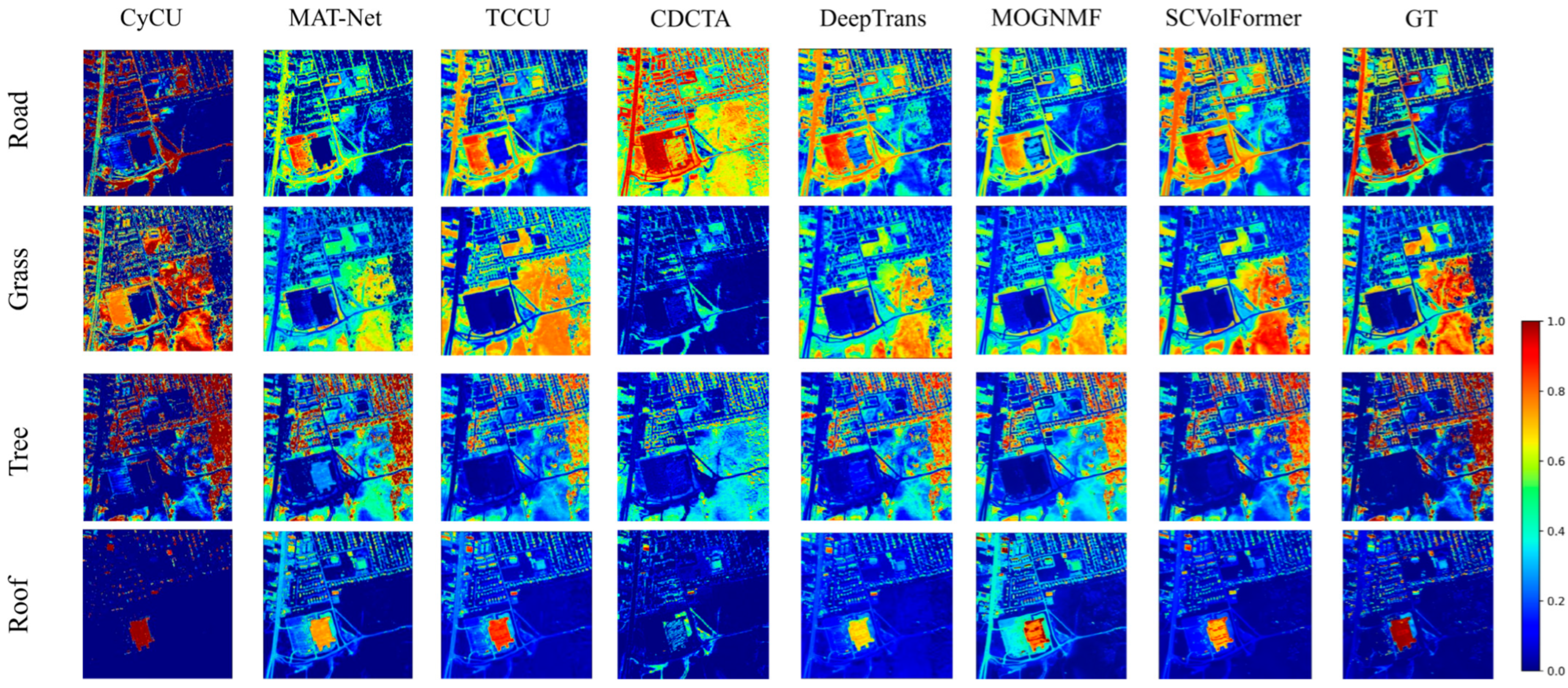
To further evaluate the performance of different methods in complex urban scenes, the abundance maps and extracted endmember spectra on the Urban dataset are visualized in Figure 13 and Figure 14. As shown in the abundance maps, the Urban dataset contains a large number of buildings, roads, vegetation, and their transition areas, resulting in more complicated spatial distributions than the previous datasets.

Figure 13. Abundance maps estimated by different unmixing methods on the Urban dataset. The GT column shows the GT abundance maps.

Figure 14. Reference signatures (red) and estimated endmember signatures (blue) by different unmixing methods on the Urban dataset.

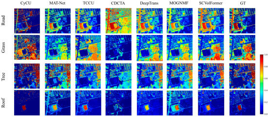
From the abundance maps, obvious differences can be observed among the compared methods. CyCU produces relatively high responses in many non-target regions, especially for the Road and Tree endmembers, making the estimated distributions noticeably different from the ground truth. MAT–Net and TCCU can recover the main spatial distribution of each endmember, but the abundance values around building boundaries and transition regions are relatively scattered. CDCTA exhibits larger deviations for the Road and Roof endmembers, where the target regions are partially enlarged or suppressed compared with the reference maps. DeepTrans and MOGNMF achieve relatively stable results, yet low-abundance responses can still be observed in several non–target regions, particularly around vegetation and building boundaries.

In contrast, the abundance maps generated by SCVolFormer are visually the closest to the ground truth. The proposed method accurately recovers the spatial distributions of the four endmembers while maintaining clearer boundaries between adjacent materials. Moreover, the abundance variation in transition regions is more consistent with the reference maps, and the responses in non-target regions remain relatively low.

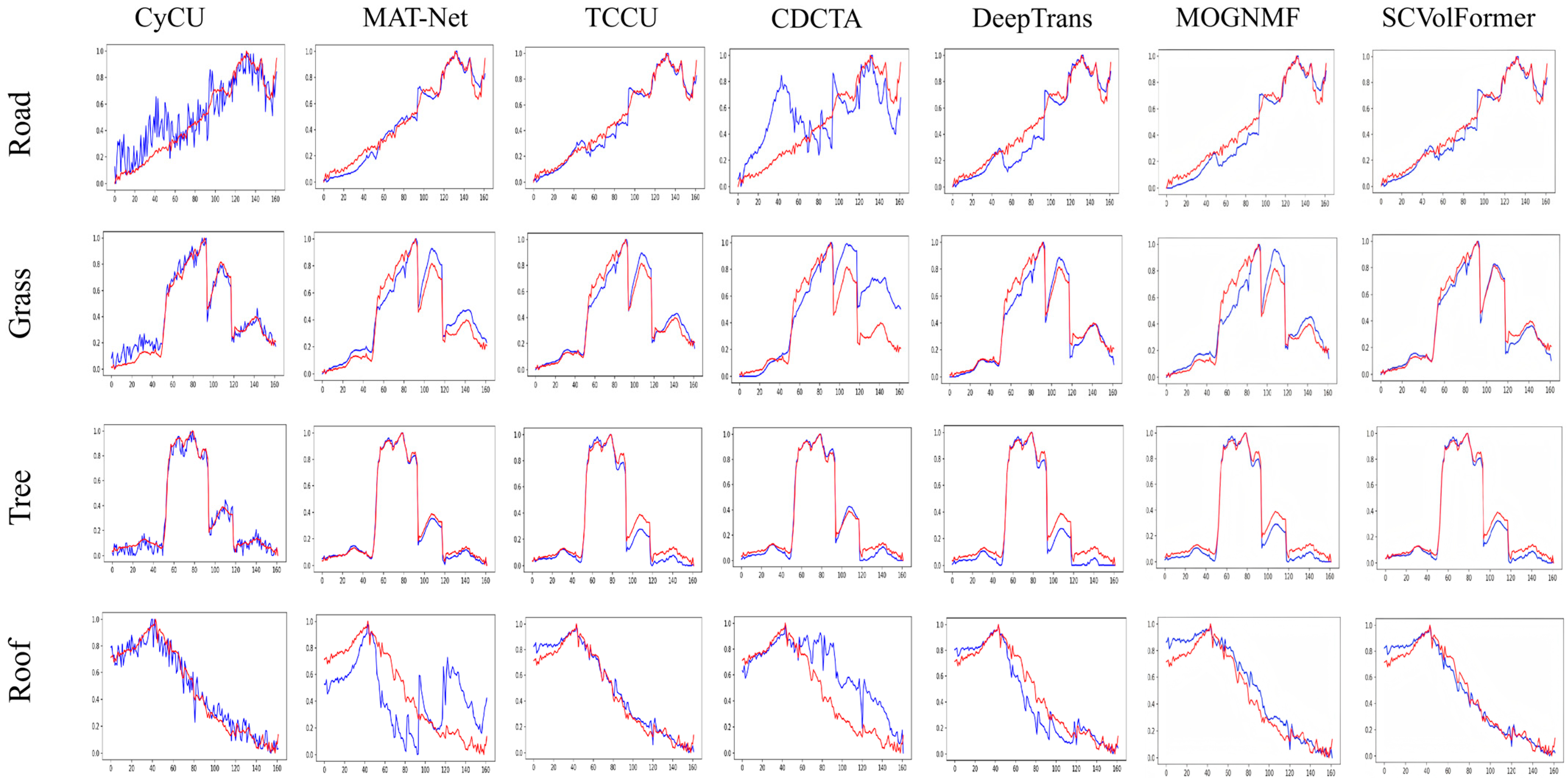
Figure 14 also presents the extracted endmember spectra of different methods. Most deep learning methods are able to capture the overall spectral trends of the endmembers, but noticeable deviations remain in several wavelength ranges. Among them, CyCU and CDCTA show relatively large fitting errors for the Road endmember, while MAT–Net, TCCU, and DeepTrans exhibit certain deviations at the local peaks and valleys of the Grass and Roof spectra. In comparison, the endmember spectra estimated by SCVolFormer are consistently closer to the reference spectra for all four endmembers. The proposed method follows the spectral variations more accurately over the entire wavelength range, demonstrating its ability to estimate both abundances and endmember signatures more precisely.

4.2.3. Visualization of Reconstruction Results

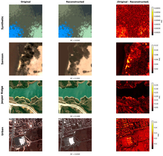
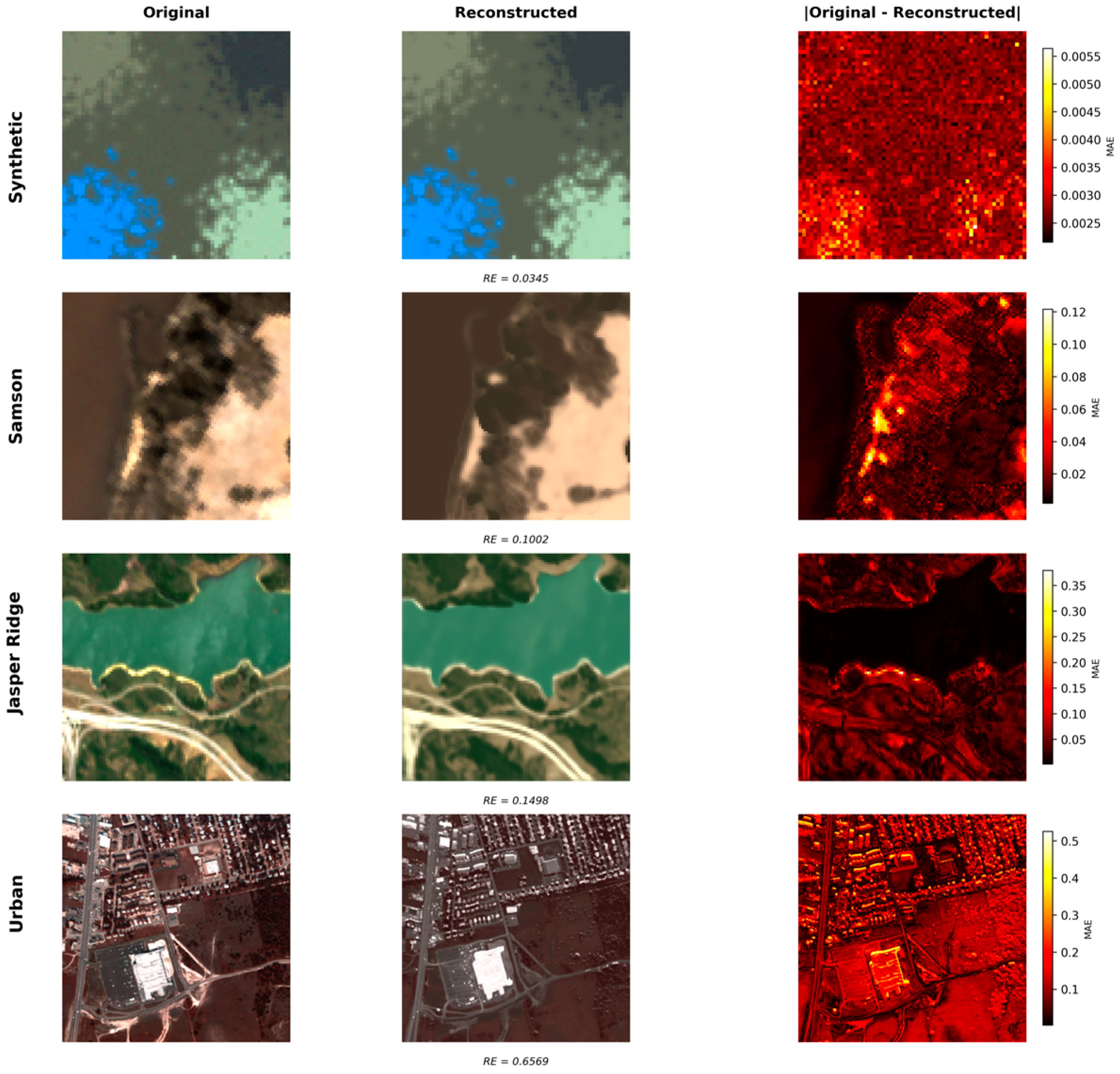
To further evaluate the reconstruction capability of SCVolFormer, additional visualization results are provided in Figure 15. The original hyperspectral images, reconstructed images, and corresponding residual maps are presented for different datasets. The residual maps are generated by calculating the band-wise averaged absolute difference between the original and reconstructed hyperspectral images.

Figure 15. Visualization of hyperspectral image reconstruction and residual maps on different datasets.

As shown in Figure 15, the reconstructed images maintain highly consistent spatial structures and visual characteristics with the original hyperspectral images across different datasets. The residual maps exhibit relatively low and spatially smooth errors in most regions, demonstrating that SCVolFormer can effectively capture the underlying spectral–spatial correlations and achieve accurate hyperspectral image reconstruction. Although larger residual responses appear in some complex regions with strong spectral variations or heterogeneous materials, the overall reconstruction error remains limited, further validating the reconstruction capability of the proposed method.

4.2.4. Ablation Experiment

To verify the effectiveness of the proposed modules, ablation experiments were conducted on the Synthetic, Samson, Jasper Ridge, and Urban datasets. The results are reported in Table 14, where SCB denotes the Spectral Consistency Block and VolLSA denotes the Volumetric Linear Self-Attention module.

Table 14. Ablation experiment on our proposed SCVolFormer with varying information enhancement on different datasets. Best results are shown in bold. Note: √ denotes that the corresponding module is used, and × denotes that the module is not used.

Module		Synthetic		Samson		Jasper Ridge		Urban
SCB	VolLSA	RMSE	SAD	RMSE	SAD	RMSE	SAD	RMSE	SAD
√	√	0.013867	0.005116	0.054661	0.046892	0.078729	0.069818	0.140484	0.1184
×	√	0.016206	0.006188	0.110558	0.074311	0.102101	0.070966	0.170359	0.139292
√	×	0.078927	0.035354	0.156731	0.0946653	0.075191	0.075028	0.226008	0.135381

As shown in Table 14, the complete SCVolFormer consistently achieves the best performance on all four datasets, demonstrating that SCB and VolLSA provide complementary improvements. On the Synthetic dataset, the complete model achieves an RMSE of 0.013867 and an SAD of 0.005116, outperforming the variants using only VolLSA or only SCB. Similar improvements are also observed on the Samson, Jasper Ridge, and Urban datasets, indicating the robustness of the proposed framework under different spectral and spatial conditions.

When SCB is removed, the performance degrades on all datasets. For example, the RMSE on the Samson dataset increases from 0.054661 to 0.110558, while the SAD on the Urban dataset rises from 0.1184 to 0.139292. This degradation is mainly attributed to the loss of spectral consistency constraints, which weakens the ability to distinguish spectrally similar materials and leads to increased spectral confusion during abundance estimation. The larger performance drop observed on real datasets indicates that SCB is particularly beneficial for handling complex spectral variations and material similarity in real hyperspectral scenes. When VolLSA is removed, the performance degradation becomes more significant. On the Synthetic dataset, the RMSE increases from 0.013867 to 0.078927, while the SAD increases from 0.005116 to 0.035354. Similar trends are observed on the Samson and Urban datasets. Without VolLSA, the model loses the capability of effectively capturing long-range spectral–spatial dependencies, resulting in weaker spatial structure preservation and blurred abundance boundaries, especially in datasets with larger spatial dimensions such as Urban.

5. Discussion

Despite the promising performance, several limitations remain in the current framework. The proposed method is mainly developed under the linear mixing model (LMM) assumption, where the observed hyperspectral signal is represented as a linear combination of endmember signatures. However, nonlinear mixing effects caused by multiple scattering and complex material interactions may occur in real-world hyperspectral scenes. Extending the proposed framework to more flexible nonlinear mixing models while maintaining physical interpretability will be an important direction for future research. In addition, spectral variability induced by illumination conditions, environmental changes, and material diversity remains a challenging issue in hyperspectral unmixing. Although SCVolFormer improves spectral consistency modeling, explicit adaptation to spectral variability has not been incorporated into the current framework. Future investigations may focus on developing adaptive spectral variability modeling strategies to further improve the robustness of the method in complex scenarios. In addition, spectral variability induced by illumination conditions, environmental changes, and material diversity remains a challenging issue in hyperspectral unmixing. Although SCVolFormer improves spectral consistency modeling, explicit adaptation to spectral variability has not been incorporated into the current framework. Future investigations may focus on developing adaptive spectral variability modeling strategies to further improve the robustness of the method in complex scenarios. Furthermore, the current evaluation is mainly conducted on widely used benchmark datasets. The extension of SCVolFormer to cross-scene applications, limited-supervision scenarios, and large-scale hyperspectral imagery requires further exploration. More efficient training strategies and scalable architectures will be investigated to improve the generalization capability and practical applicability of the proposed framework.

6. Conclusions

This paper proposed SCVolFormer, a Spectral Consistency–guided Transformer framework for hyperspectral unmixing. A Spectral Consistency Block (SCB) was designed to preserve band-wise spectral consistency based on the linear mixing model, while a Volumetric Linear Self-Attention (VolLSA) module was introduced to jointly model long-range spectral–spatial dependencies with an explicit spectral positional prior. Extensive experiments on one synthetic dataset and three real hyperspectral datasets demonstrated that the proposed method consistently outperformed several state-of-the-art methods in both abundance estimation and endmember extraction. Ablation studies further verified the effectiveness of SCB and VolLSA. Future work will investigate nonlinear mixing models and lightweight Transformer architectures to further improve the efficiency and generalization ability of hyperspectral unmixing in more challenging real-world scenarios.

References

- Shaw, G.A.; Burke, H.K. Spectral imaging for remote sensing. Linc. Lab. J. 2003, 14, 3–28. [Google Scholar]
- Jin, Q.; Ma, Y.; Mei, X.; Dai, X.; Li, H.; Fan, F. Gaussian mixture model for hyperspectral unmixing with low–rank representation. In Proceedings of the IGARSS 2019-2019 IEEE International Geoscience and Remote Sensing Symposium, Yokohama, Japan, 28 July–2 August 2019; IEEE: New York, NY, USA, 2019; pp. 294–297. [Google Scholar]
- Zhang, X.; Cao, L.; Ge, J.; Feng, R.; Han, W.; Huang, X.; Wang, S.; Wang, Y. Hyperspectral Unmixing–Based Remote Sensing Inversion of Multiple Heavy Metals in Mining Soils: A Case Study of the Lengshuijiang Antimony Mine, Hunan Province. Remote Sens. 2026, 18, 767. [Google Scholar] [CrossRef] [Scilit]
- Fu, B.; Shi, P.; Fu, H.; Ninomiya, Y.; Du, J. Geological Mapping Using Multispectral Remote Sensing Data in the Western China. In Proceedings of the IEEE International Geoscience Remote Sensing Symposium, Yokohama, Japan, 28 July–2 August 2019; IEEE: New York, NY, USA, 2019; pp. 5583–5586. [Google Scholar]
- Guan, Q.; Qiao, S.; Feng, S.; Du, W. Investigation of Peanut Leaf Spot Detection Using Superpixel Unmixing Technology for Hyperspectral UAV Images. Agriculture 2025, 15, 597. [Google Scholar] [CrossRef] [Scilit]
- Barma, S.; Damarla, S.; Tiwari, S. Semi–Automated Technique for Vegetation Analysis in Sentinel–2 Multi–Spectral Remote Sensing Images Using Python. In Proceedings of the 4th International Conference. Electronic Communications Aerospace Technology, Coimbatore, India, 5–7 November 2020; IEEE: New York, NY, USA, 2020; pp. 946–953. [Google Scholar]
- Li, F.; Liu, D.; Guo, X.; Guo, X.; Zhang, Z.; Martin, F.L.; Lu, A. Identification and visualization of environmental microplastics by Raman imaging based on hyperspectral unmixing coupled machine learning. J. Hazard. Mater. 2024, 465, 133336. [Google Scholar] [CrossRef] [Scilit] [PubMed]
- Karoui, M.S.; Benhalouche, F.Z.; Deville, Y.; Djerriri, K.; Briottet, X.; Houet, T.; Le Bris, A.; Weber, C. Partial Linear NMF–Based Unmixing Methods for Detection and Area Estimation of Photovoltaic Panels in Urban Hyperspectral Remote Sensing Data. Remote Sens. 2019, 11, 2164. [Google Scholar] [CrossRef] [Scilit]
- Chen, F.; Wang, K.; Van de Voorde, T.; Tang, T.F. Mapping urban land cover from high spatial resolution hyperspectral data: An approach based on simultaneously unmixing similar pixels with jointly sparse spectral mixture analysis. Remote Sens. Environ. 2017, 196, 324–342. [Google Scholar] [CrossRef] [Scilit]
- Lin, H.; Zhang, X. Retrieving the hydrous minerals on Mars by sparse unmixing and the Hapke model using MRO/CRISM data. Icarus 2017, 288, 160–171. [Google Scholar] [CrossRef] [Scilit]
- Ertürk, A.; Erten, E. Unmixing of pollution–associated sea snot in the near surface after its outbreak in the Sea of Marmara using hyperspectral PRISMA data. IEEE Geosci. Remote Sens. Lett. 2023, 20, 5501705. [Google Scholar] [CrossRef] [Scilit]
- Rehman, A.U.; Qureshi, S.A. A review of the medical hyperspectral imaging systems and unmixing algorithms’ in biological tissues. Photodiagnosis Photodyn. Ther. 2021, 33, 102165. [Google Scholar] [CrossRef] [Scilit] [PubMed]
- Zhao, J.; Zhou, B.; Wang, G.; Ying, J.; Liu, J.; Chen, Q. Spectral Camouflage Characteristics and Recognition Ability of Targets Based on Visible/Near–Infrared Hyperspectral Images. Photonics 2022, 9, 957. [Google Scholar] [CrossRef] [Scilit]
- Deshpande, V.S.; Bhatt, J.S. A practical approach for hyperspectral unmixing using deep learning. IEEE Geosci. Remote Sens. Lett. 2021, 19, 5511505. [Google Scholar] [CrossRef] [Scilit]
- Wang, M.; Yang, K.; Lu, J.; Liu, W.; Zeng, T. A Spectral Variability and Class–Constrained Diffusion Model for Unsupervised Hyperspectral Unmixing. Remote Sens. 2026, 18, 1483. [Google Scholar] [CrossRef] [Scilit]
- Wang, C.; Gao, J.; Zhu, F.; Halimi, A.; Richard, C. DTU–Net: A multi–scale dilated transformer network for nonlinear hyperspectral unmixing. IEEE Trans. Geosci. Remote Sens. 2026, 64, 5502917. [Google Scholar] [CrossRef] [Scilit]
- Zou, J.; Qu, H.; Zhang, P. Conventional to Deep Learning Methods for Hyperspectral Unmixing: A Review. Remote Sens. 2025, 17, 2968. [Google Scholar] [CrossRef] [Scilit]
- Deán–Ben, X.L.; Deliolanis, N.C.; Ntziachristos, V.; Razansky, D. Fast unmixing of multispectral optoacoustic data with vertex component analysis. Opt. Lasers Eng. 2014, 58, 119–125. [Google Scholar] [CrossRef] [Scilit]
- Pu, H.; Chen, Z.; Wang, B.; Xia, W. Constrained least squares algorithms for nonlinear unmixing of hyperspectral imagery. IEEE Trans. Geosci. Remote Sens. 2014, 53, 1287–1303. [Google Scholar] [CrossRef] [Scilit]
- Zhao, M.; Gao, T.; Chen, J.; Chen, W. Hyperspectral unmixing via nonnegative matrix factorization with handcrafted and learned priors. IEEE Geosci. Remote Sens. Lett. 2021, 19, 5501905. [Google Scholar] [CrossRef] [Scilit]
- Dong, L.E.; Yuan, Y.; Luxs, X. Spectral–spatial joint sparse NMF for hyperspectral unmixing. IEEE Trans. Geosci. Remote Sens. 2020, 59, 2391–2402. [Google Scholar] [CrossRef] [Scilit]
- Chen, H.; Liu, L.; Xiu, X.; Liu, W. Adaptive multi–order graph regularized NMF with dual sparsity for hyperspectral unmixing. IEEE J. Sel. Top. Appl. Earth Obs. Remote Sens. 2025, 18, 22121–22136. [Google Scholar] [CrossRef] [Scilit]
- Yang, T.; Li, S.; Song, M.; Yu, C.; Bao, H. Low–rank and sparse NMF based on compression and correlation sensing for hyperspectral unmixing. Infrared Phys. Technol. 2024, 141, 105464. [Google Scholar] [CrossRef] [Scilit]
- Qian, Y.; Xiong, F.; Zeng, S.; Zhou, J.; Tang, Y.Y. Matrix–vector nonnegative tensor factorization for blind unmixing of hyperspectral imagery. IEEE Trans. Geosci. Remote Sens. 2016, 55, 1776–1792. [Google Scholar] [CrossRef] [Scilit]
- Su, Y.; Zhu, Z.; Gao, L.; Plaza, A.; Li, P.; Sun, X. DAAN: A deep autoencoder–based augmented network for blind multilinear hyperspectral unmixing. IEEE Trans. Geosci. Remote Sens. 2024, 62, 5512715. [Google Scholar] [CrossRef] [Scilit]
- Gao, L.; Han, Z.; Hong, D.; Zhang, B.; Chanussot, J. CyCU–Net: Cycle–consistency unmixing network by learning cascaded autoencoders. IEEE Trans. Geosci. Remote Sens. 2021, 60, 5503914. [Google Scholar] [CrossRef] [Scilit]
- Xiong, F.; Zhou, J.; Ye, M.; Lu, J.; Qian, Y. NMF–SAE: An interpretable sparse autoencoder for hyperspectral unmixing. In Proceedings of the ICASSP 2021-2021 IEEE International Conference on Acoustics, Speech and Signal Processing (ICASSP), Toronto, ON, Canada, 6–11 June 2021; IEEE: New York, NY, USA, 2021; pp. 1865–1869. [Google Scholar]
- Zhao, M.; Chen, J.; Dobigeon, N. AE–RED: A hyperspectral unmixing framework powered by deep autoencoder and regularization by denoising. IEEE Trans. Geosci. Remote Sens. 2024, 62, 5512115. [Google Scholar] [CrossRef] [Scilit]
- Xu, M.; Xu, J.; Liu, S.; Sheng, H.; Yang, Z. Multiscale convolutional mask network for hyperspectral unmixing. IEEE J. Sel. Top. Appl. Earth Obs. Remote Sens. 2024, 17, 3687–3700. [Google Scholar] [CrossRef] [Scilit]
- Hong, D.; Gao, L.; Yao, J.; Yokoya, N.; Chanussot, J.; Heiden, U.; Zhang, B. Endmember–guided unmixing network (EGU–Net): A general deep learning framework for self–supervised hyperspectral unmixing. IEEE Trans. Neural Netw. Learn. Syst. 2021, 33, 6518–6531. [Google Scholar] [CrossRef] [Scilit] [PubMed]
- Tulczyjew, L.; Kawulok, M.; Longépé, N.; Le Saux, B.; Nalepa, J. A multibranch convolutional neural network for hyperspectral unmixing. IEEE Geosci. Remote Sens. Lett. 2022, 19, 6011105. [Google Scholar] [CrossRef] [Scilit]
- Kong, F.; Chen, M.; Li, Y.; Li, D.; Zheng, Y. Deep interpretable fully CNN structure for sparse hyperspectral unmixing via model–driven and data–driven integration. IEEE Trans. Geosci. Remote Sens. 2023, 61, 5527716. [Google Scholar] [CrossRef] [Scilit]
- Rasti, B.; Koirala, B.; Scheunders, P.; Chanussot, J. MiSiCNet: Minimum simplex convolutional network for deep hyperspectral unmixing. IEEE Trans. Geosci. Remote Sens. 2022, 60, 5522815. [Google Scholar] [CrossRef] [Scilit]
- Zhang, J.; Zhang, X.; Fan, J.; Meng, H. 3D–CNN and semi–supervised based network for hyperspectral unmixing. Int. J. Remote Sens. 2024, 45, 168–191. [Google Scholar] [CrossRef] [Scilit]
- Rasti, B.; Koirala, B.; Scheunders, P.; Ghamisi, P. UnDIP: Hyperspectral unmixing using deep image prior. IEEE Trans. Geosci. Remote Sens. 2021, 60, 5504615. [Google Scholar] [CrossRef] [Scilit]
- Elkholy, M.M.; Moustafa, M.S.; ElSayad, D.; Ebied, H.M. UnTrNet: A transformer–based hyperspectral change detection using abundance maps. Int. J. Data Sci. Anal. 2026, 22, 112. [Google Scholar] [CrossRef] [Scilit]
- Ghosh, P.; Roy, S.K.; Koirala, B.; Rasti, B.; Scheunders, P. Hyperspectral unmixing using transformer network. IEEE Trans. Geosci. Remote Sens. 2022, 60, 5535116. [Google Scholar] [CrossRef] [Scilit]
- Chen, J.; Yang, C.; Zhang, L.; Yang, L.; Bian, L.; Luo, Z.; Wang, J. TCCU–Net: Transformer and CNN collaborative unmixing network for hyperspectral image. IEEE J. Sel. Top. Appl. Earth Obs. Remote Sens. 2024, 17, 8073–8089. [Google Scholar] [CrossRef] [Scilit]
- Wang, P.; Liu, R.; Zhang, L. Mat–net: Multiscale aggregation transformer network for hyperspectral unmixing. IEEE Trans. Geosci. Remote Sens. 2024, 62, 5538115. [Google Scholar] [CrossRef] [Scilit]
- Yang, Y.; Wang, Y.; Liu, T. CDCTA: Cascaded dual–constrained transformer autoencoder for hyperspectral unmixing with endmember variability and spectral geometry. J. Appl. Remote Sens. 2024, 18, 026502. [Google Scholar] [CrossRef] [Scilit]
- Su, Y.; Gao, L.; Plaza, A.; Sun, X.; Jiang, M.; Yang, G. SRViT: Self–supervised relation–aware vision transformer for hyperspectral unmixing. IEEE Trans. Neural Netw. Learn. Syst. 2025, 36, 17585–17598. [Google Scholar] [CrossRef] [Scilit] [PubMed]
- Yu, D.; Gao, Z. VolFormer: Explore more comprehensive cube interaction for hyperspectral image restoration and beyond. In Proceedings of the Computer Vision and Pattern Recognition Conference; IEEE: New York, NY, USA, 2025; pp. 28091–28101. [Google Scholar]
- Gao, W.; Zhang, Y.; Akoudad, Y.; Chen, J. MSSF–Net: A multimodal spectral–spatial feature fusion network for hyperspectral unmixing. IEEE Trans. Geosci. Remote Sens. 2025, 63, 5511515. [Google Scholar] [CrossRef] [Scilit]
- Lin, Q.; Liu, C.; Han, D.; Liu, W.; Bo, Z.; Zhang, P. A Hapke Physics–Guided Deep Autoencoder for Lunar Hyperspectral Unmixing. Remote Sens. 2026, 18, 1123. [Google Scholar] [CrossRef] [Scilit]
- Shu, S.; Huang, T.Z.; Huang, J.; Vivone, G. Physics–Guided Vision Transformer Network With Tokens Complementarity for Hyperspectral Unmixing. IEEE Trans. Geosci. Remote Sens. 2026, 64, 5509221. [Google Scholar] [CrossRef] [Scilit]
- Guo, H.; Li, J.; Dai, T.; Quyang, Z.; Ren, X.; Xia, S.T. Mambair: A simple baseline for image restoration with state–Space model. In European Conference on Computer Vision; Springer Nature: Cham, Switzerland, 2024; pp. 222–241. [Google Scholar] [CrossRef] [Scilit]
- Li, C.; Hong, D.; Zhang, B.; Chanussot, J. Im2State: Image–to–state Mamba for hyperspectral and multispectral image fusion. Inf. Fusion 2026, 134, 104385. [Google Scholar] [CrossRef] [Scilit]
- Chen, D.; Zhang, J.; Li, J. UNMamba: Cascaded spatial–spectral mamba for blind hyperspectral unmixing. IEEE Geosci. Remote Sens. Lett. 2025, 22, 5502405. [Google Scholar] [CrossRef] [Scilit]
- Hong, D.; Zhang, B.; Li, X.; Li, Y.; Li, C.; Yao, J.; Yokoya, N.; Hao, L.; Ghamisi, P.; Jia, X.; et al. SpectralGPT: Spectral remote sensing foundation model. IEEE Trans. Pattern Anal. Mach. Intell. 2024, 46, 5227–5244. [Google Scholar] [CrossRef] [Scilit] [PubMed]
- Tao, X.; Paoletti, M.E.; Han, L.; Wu, Z.; Ren, P.; Plaza, J.; Haut, J.M. A new deep convolutional network for effective hyperspectral unmixing. IEEE J. Sel. Top. Appl. Earth Obs. Remote Sens. 2022, 15, 6999–7012. [Google Scholar] [CrossRef] [Scilit]
- Hu, S.; Li, H. Hyperspectral unmixing with multi–scale convolution attention network. IEEE J. Sel. Top. Appl. Earth Obs. Remote Sens. 2024, 17, 2531–2542. [Google Scholar] [CrossRef] [Scilit]
- Zhao, M.; Wang, M.; Chen, J.; Rahardja, S. Hyperspectral unmixing for additive nonlinear models with a 3–D–CNN autoencoder network. IEEE Trans. Geosci. Remote Sens. 2022, 60, 5509415. [Google Scholar] [CrossRef] [Scilit]
- Wang, X.; Zhong, Y.; Zhang, L.; Xu, Y. Spatial group sparsity regularized nonnegative matrix factorization for hyperspectral unmixing. IEEE Trans. Geosci. Remote Sens. 2017, 55, 6287–6304. [Google Scholar] [CrossRef] [Scilit]
Disclaimer/Publisher’s Note: The statements, opinions and data contained in all publications are solely those of the individual author(s) and contributor(s) and not of MDPI and/or the editor(s). MDPI and/or the editor(s) disclaim responsibility for any injury to people or property resulting from any ideas, methods, instructions or products referred to in the content. |
© 2026 by the authors. Licensee MDPI, Basel, Switzerland. This article is an open access article distributed under the terms and conditions of the Creative Commons Attribution (CC BY) license.