


Abstract
We introduce the two-point propagation field (TPPF)—a real-valued, phase-sensitive quantity defined as the functional derivative of the single-photon detection probability with respect to an infinitesimal opaque perturbation placed between the source and detection slits. The TPPF is analytically derived and shown to exhibit a stable, high-frequency sinusoidal structure with periods of 4~7 nm near the X-ray detection slit. This structure enables shot-noise-limited displacement detection with ∼200 pm precision for 6 keV X-rays using total photon counts on the order of 1 × and detector photon counting as low as 287. Beyond displacement detection, the TPPF physically performs a Fourier–Radon transformation of the projection data, providing a pathway to non-iterative frequency-domain tomography. Two conceptual strategies—a central blocker and off-axis multi-slit arrays—are estimated to lower the required incident photon budget by more than one order of magnitude each, yielding combined reductions of two to three orders of magnitude with near-term detector development. The TPPF concept, originally developed in a perturbative study of single-particle propagation, bridges quantum measurement questions with practical high-resolution X-ray physics. This work provides the foundational physics required for future discrete sampling and 3D numerical reconstruction algorithms.
1. Introduction and Motivation
We outline a concept—the two-point propagation field (TPPF)—that may provide a practical basis for achieving shot-noise-limited X-ray displacement detection with ∼200 pm precision for existing synchrotron beamlines and practical slit–comb samples. This approach addresses the relative sample-beam motion that restricts resolution to ∼4 nm [1]. The method is based on the two-point propagation field (TPPF), a real-valued, phase-sensitive function derived from perturbative analysis of single-particle propagation. TPPF is derived from the perturbative response of detection rates to localized perturbations—such as placing a thin opaque pin to block the wave—at intermediate points along the photon propagation path between a source slit and a detection slit. This quantity, referred to as the two-point propagation field (TPPF), was introduced and derived in detail in a recent theoretical study [2], where it was originally termed the “perturbative function”.
The central idea is that this function captures projection-like information about a sample’s internal structure by encoding how the count rate at a detector changes when the wave is perturbed by a pin at different points. When we replace the perturbation pin with a sample as the perturbation, the detection rate becomes a function of the position and the angle of the sample orientation. The function is a convolution between the TPPF and the sample’s structural function. The result is a stable, reproducible function that varies with the scan position and angle of the sample, and may be viewed as analogous to the projection data used in Radon transform-based reconstruction techniques. However, in this case, the measured signal is directly related to the Fourier transform of the Radon transform due to the high-frequency phase information inherent in the TPPF.
Although this work does not address reconstruction techniques, the structure of the TPPF suggests a possible path toward extending classical tomographic methods to single-particle quantum systems—particularly in efforts to resolve nanometer-scale structural features. This paper presents the TPPF formula, its physical interpretation, and a proposed connection to projection-based 3D tomography [3,4]. The objective of this work is to establish a clear framework for researchers in 3D imaging and X-ray science and to explore whether the method can be experimentally tested and integrated into an existing tomographic method. As the first step in this direction, the analysis leads to practical shot-noise-limited displacement detection precision of ∼200 pm for existing synchrotron beamlines and practical comb/slit geometries. Such precision enables lensless, counting-based detection that requires stability only over the final 0.5 mm propagation distance, utilizing total photon counts of to , readily achievable at synchrotron or XFEL beamlines, depending on slit configurations.
This step itself is useful for the advancement of X-ray tomography because the motion between the X-ray beam and the sample of order of 4 nm is one of the limitations of tomography resolution [1]. By encoding high-frequency phase information akin to a Fourier-transformed Radon projection (Section 3), the TPPF supports reconstruction of internal structures at nanometer scales, offering a pathway to lower-dose imaging compared to conventional ptychography or burst methods. This not only facilitates experimental validation of the TPPF but also reduces radiation damage in biological samples, potentially by more than one order of magnitude, through strategies like central blockers or off-axis slit arrays, as explored in Section 5.
Section 2 introduces the two-point propagation function (TPPF). Section 3 examines its connection to the Radon transform and 3D tomography. In Section 4, we illustrate how to apply the calculation steps for the X-ray picometer displacement detection to an example in a 6 keV X-ray case. Section 5 describes ongoing work to significantly reduce the photon count requirements for achieving the target sensitivity. Section 6 discusses the relation between TPPF and quantum measurement during the free-space propagation between the source and the detector slit. Section 7 is a discussion on the groundbreaking aspects of the TPPF framework. Section 8 is the conclusion.
This work is approached from a theoretical standpoint, using broadly referenced parameters to assess the compatibility of a picometer X-ray displacement detection and nanometer-resolution 3D tomography with existing technology. Although not based on direct experience with experimental tomography or biological imaging, the analysis intends to provide a foundation for shared exploration and further evaluation by experts in these areas.
2. Description of the Experiment to Measure the Two-Point Propagation Field
2.1. TPPF and Its Physical Interpretation
As illustrated in Figure 1a, we analyze the wave function evolution of a particle when it propagates through free space in the longitudinal z-direction from a thin entrance slit 1 to a detector behind a thin exit detector slit 2 to find the information about whether the wave function collapse occurs at entrance slit 1 or exit detector slit 2. The slits are parallel to the y-axis (perpendicular to the plane of the figure). The x-axis is vertical in the figure. Between the slits, the wave function must follow the Schrödinger equation because the only non-unitary (irreversible) process is at the slits. Only the particles that pass through the slits are selected and detected. The probability of a particle found between and is a constant independent of z due to particle number conservation. We insert a thin pin between the two slits at position to cut off the wave function as a perturbation. When , there is no pin. When within a thin section around a point at (x,z), it represents a thin pin. When in an extended area, it becomes a sample as a perturbation. The caption for Figure 1a gives the notations.
Figure 1.
(a) Experimental geometry (not to scale). The wave functions at slits 1 and 2 at with apertures , corresponding transverse displacements in the x-direction, and a pin at of width . The distances between the slits and the pin are and The longitudinal axis is the z-axis, the x-axis is vertical in this figure. The slits are perpendicular to the plane of the figure, parallel to the y-axis. We use , , and to represent the wave function at the entrance, the pin, and the exit, respectively. The subscripts a and b represent before and after detector slit 2. and represent the effect of the slits such that . If we choose the slit with the hard-edged opening, and would be zero outside the slits and equal to 1 within the slits. To simplify the calculation, we assume they are Gaussian with peak value 1, except that we choose to normalize as . The pin profile is when it is removed. When inserted, ; the effective width (equivalent hard-edged slit width) is . (b) The wave function of a single particle spreads over a wide region after emission and collapses instantaneously upon detection.
In Figure 1a, we study the effect of a perturbation on the counting rate and calculate the ratio of the counting rate change over the perturbation. As the perturbation approaches zero, the ratio becomes the functional derivative of the counting rate over the perturbation . This perturbative function is independent of perturbation; it is a real-valued function containing high-resolution phase information, determined solely by the two-slit geometry in our 2D study, as demonstrated later. It can be measured with high precision and reproducibility, and it uniquely characterizes the individual event of a particle propagating between the two slits. Unlike a probability amplitude, it manifests as a stable, reproducible structure corresponding to a physically meaningful propagation quantity exhibiting high-resolution fringes, which we define as the two-point propagation field (TPPF). The TPPF does not correspond to a probability distribution. While the wave function describes an ensemble of possible detection outcomes, the TPPF characterizes the process underlying a single detection—a realization selected according to the Born rule.
In Appendix B, we outline a derivation of the calculation of TPPF using the basics of quantum mechanics. Since in this work we consider X-ray 3D tomography, for the case in Figure 1a and for sufficiently long and narrow slits and the pin, we neglect the y dependence and assume a 2D Maxwell equation
Because we do not consider polarization, we just use to denote any component of the electromagnetic field. We assume , ; take the paraxial approximation: ||, ||, and we get the 1D Schrödinger equation . is the slowly varying amplitude and phase of the wave function. We can characterize the experiment by specifying the wavelength only. The Green’s function from entrance slit 1 to detector slit 2 is
The initial wave function is the Gaussian profile of entrance slit 1, is for detector slit 2. Our analysis shows that for the narrow slits we considered, replacing the Gaussian profile by a hard-edge profile of width would only cause a negligible difference. The Gaussian profile allows us to derive a simple analytical result, as described in Section 2.2.
In the derivation of the TPPF, the Green’s functions ),) are given by replacing the corresponding variables in Equation (2). When wave function at entrance slit 1 is normalized as , applying the property of the Green’s function without the pin, the wave function at the exit of detector slit 2 is . When there is a perturbation of a pin, the wave function after detector slit 2 is
Because within the thin section the increment for infinitesimal is
Thus, the functional derivative of over the perturbation is
The TPPF is the functional derivative of the detection probability over the perturbation , and we define the complex part of TPPF as . We have
Applying Equation (4), we have the complex TPPF
The last step shows that there is a simple relation between TPPF and the probability , i.e.,
Thus, the integration of TPPF over x is not the probability but twice of it. An important observation is that is a function of z, i.e., the position z of the pin, but is independent of z and represents the particle number conservation during the free propagation in free space. Although the two-point propagation field (TPPF) is not positive-definite, its integral over space yields a conserved total probability. When normalized and scaled by , it acquires the dimensions of energy density and integrates to the particle’s total energy. The possibility of local negative values is not without precedent; similar behaviors occur in quantum field theory, such as in the Casimir effect [5]. We therefore interpret the scaled TPPF as a generalized energy density associated with the spatial structure of single-particle propagation.
Since is the real part of the complex-valued , its imaginary part—and thus the full complex derivative—can be readily obtained via a Hilbert transform. As is standard in Fourier analysis [6], this is accomplished simply by multiplying the Fourier coefficients of the real part by a constant according to the sign of the frequency (see Appendix A), followed by an inverse Fourier transform. As we shall show, and are entirely different functions: is widespread as illustrated in Figure 1b; however, becomes widespread only between the two slits and finally converges into detector slit 2. This answers the fundamental question: the evolution of the energy distribution is continuous without sudden collapse at the detector, as suggested by the TPPF model, even though the wave function collapses at the instant of the detection. represents a statistical distribution of the ensemble, while TPPF represents an individual realization of the ensemble.
2.2. The Expression of TPPF and Its Difference from the Wave Function
This simple relation between TPPF and the counting rate in Equation (7) is used in simplifying the derivation of the complex TPPF Equation (6) in Appendix B. The result for the counting rate (i.e., the probability) and the explicit complex-valued TPPF is simpler when expressed in terms of a few scaled parameters in Figure 1 for slit width and longitudinal position: , :
Here, are the transverse displacements of the slits in Figure 1a, and , . For the next discussion on the tomography, we only consider the case of ; thus , and hence, TPPF is characterized mainly by the probability and that provide the information about the distribution width, fringe spacing, frequency bandwidth, etc., of TPPF.
In the example in Figure 2a, we display the TPPF using a color scale for a case of nm (2.29 kev X-ray), with the setup parameters in Figure 1. The red contour in Figure 2a is also plotted as the contour of the main peak for the case of m in Figure 3, where we show several different contours of the main peaks for m, respectively, to show the different realizations of the ensemble represented by the Schrödinger equation solution; the wave function with initial condition .
Figure 2.
For a setup in Figure 1a, take = 0.541 nm, = 0.8 nm, = 0.5 m, L = 0.5 m, and L-z = 0.5 mm. (a): vs. in color scale for = 50 m, = 9.47 × 10⁻⁶. Some elliptical patterns are artifacts due to the limited number of points of the plot and the nearly periodic structure of the function . The patterns change with the number of points in the plot, but it is hard to avoid, even with pixels increased to in the plot. (b): A narrow region within 2 mm from detector slit 2 in (a) showing the details not visible in (a). The detailed fringe structure is not visible in this plot because it is visible only when magnified, as given in the following (c,d) plots. The region between the two white lines (45 is given in (c) with details. The hardly visible white dot, which is too small to be recognized as a box, indicates the region (pointed to by the arrow in (b)) shown in (d) with fringe details. (c): The region (45 indicated by the two white lines in (b). (d): The region indicated in (b) by an arrow as a white dot in a box size of (60 shows the fringe structure. The most pronounced feature is that the amplitude ( indicated by the color scale is comparable to the peak amplitude in (c).
Figure 3.
The contours of . The colored lines are the centroids for m, respectively. The cyan-colored contours represent the contours of the main peaks of TPPF for various . here is the distance from the centroid to the point with a phase shift from the centroid by . For m, this contour corresponds to the red-colored region in Figure 2a. As a comparison, the RMS of the wave function is the thick dashed cyan line showing that its width continues to spread until the end.
Figure 2b–d show several regions in Figure 2a near exit detector slit 2 with details important for the next micro-tomography discussion. In particular, Figure 2b shows that the evolution of the TPPF is continuous from z = 0.498 m to Z = 0.5 m at the exit.
To compare TPPF with , the RMS of is shown in Figure 3 as the thick dashed cyan line, showing that its width continues to spread until the exit screen. Figure 3 shows the contours of TPPF’s central peak emitted from entrance slit 1 with the shape of a spindle projected in different directions; their width increases to a maximum in the middle at about 0.25 m from the end at 0.5 m. The width of the central peak decreases after the maximum and finally, without a lens or focusing device, converges into the end detector slits. When detector slit 2 is much narrower than entrance slit 1, as for the case of Figure 2, the two sides of the central peaks are wave packets with increasing width like the width of , until very close to the exit detector slit 2 within a few hundreds μm, where they converge rapidly into detector slit 2, as shown in Figure 2b,c.
The rapid convergence is evident in Figure 2b; in particular, it reveals a large effective convergence angle—even though this is free-space propagation without any focusing. This behavior highlights the influence of the exit slit boundary condition on the propagation of a photon wave packet: the presence of the exit slit, which ultimately transmits the energy , significantly affects the evolution of the wave packet as it approaches the slit.
In the analysis of the 1D Schrödinger equation , we use the transformation to study only monochromatic photons. When we introduce energy bandwidth and study the pulse structure of the wave packet, we should be able to analyze the time-dependent behavior of the photon wave packet and further explore how the exit slit influences the convergence process. This would be an important issue to be studied.
We now discuss the relation and difference between the two functions and the TPPF . Figure 1b shows is more like a water wavefront propagating in a pond while the different wave packets of various are more like projectiles as shown in Figure 3. These projectiles, shooting into different directions, have detailed phase information as visible fringes illustrated in Figure 2c,d. This observation leads to the conclusion that represents a statistical distribution of the ensemble, and represents an individual realization of the ensemble. The main point is that the evolution of TPPF in Figure 2b further clarified the answer to a fundamental question to be addressed later in Section 7: we understand that it represents a continuous evolution of the energy distribution , unlike the sudden discontinuous collapse of the probability amplitude at the exit slit.
In Figure 2, we showed only one case of a slit 2 off-axis by m. To see how the TPPF profile changes when the slit 2 position is moved, we plot the contours of the TPPF for four different . The contour is represented by the width of the first peak of TPPF, exemplified as the first half phase shift point in the TPPF at both sides of the TPPF center . As shown in Figure 3, the TPPF always points to slit 2 at when we move it because the detected photon has to go into slit 2, and each measurement during the scan of the TPPF profile always only registers those photons that happen to be detected by slit 2, wherever it is. As a result, as we move slit 2, the TPPF behaves like a projectile aimed at slit 2. This ‘projectile’ possesses a finite width (the TPPF profile) and is not merely a geometric line or trace. Thus, it does not represent a classical trajectory; rather, it behaves like a wave packet that converges into slit 2 because we are specifically selecting only those photons that arrive at that detector location.
To compare TPPF with the wave function , we plot the thick cyan dashed line to represent its RMS width. The wave function, unlike TPPF, evolves wider and wider until the exit screen, where it has widely spread. Thus, the wave function squared represents the probability distribution of an ensemble of photons. In comparison, while the wave function describes an ensemble of possible detection outcomes, each TPPF for any given characterizes the process underlying a single detection—a realization selected according to the Born rule, as we will later discuss in Section 6.
Another important meaning of Figure 3 is to show the similarity of the TPPF profiles at different slit 2 positions . Even though the angular directions in Figure 3 seem to span a large angle, the actual span angle is much smaller because the vertical scale is significantly smaller than the horizontal scale. This means different slit 2 positions can provide different spatial frequency signals at different phases. Thus, within one exposure, two detectors at two different slit 2 positions can immediately provide the position information, while a detector array will significantly reduce the number of photons required for displacement detection or tomography scan, as will be discussed in Section 2.4, Section 3 and Section 5.
2.3. Explore Possible Application to Microscopy, Envelope Width , First-Phase Shift Fringe Spacing , and the Number of Fringes Within
Further examination of the details in Figure 2a indicates that the high-resolution fine fringes with significant amplitude become hardly visible near end detector slit 2 because when the pin position z becomes close to detector slit 2 of narrow width , the fringe spacing becomes too narrow to be visible and needs a detailed plot. Figure 2d shows that when mm, even at m, i.e., m away from the centroid m, the amplitude of oscillation is still at , almost the same as the peak value at . These details indicate a possible application of TPPF in microscopy. To explore further, we consider the X-ray wavelength at nm and apply Equation (8) to a finite pin width of 3 nm. The relative counting rate is given by the convolution of the TPPF with the pin function, which is assumed to have a Gaussian profile, . Since TPPF is the functional derivative of the counting rate with respect to the perturbation , we have the counting rate change as
Here, the left-hand side of Equation (9) expresses the general convolution relation defining the TPPF response to an arbitrary perturbation , while the right-hand side gives its explicit evaluation for a Gaussian pin profile, which is used for numerical illustration and for plotting Figure 4. When the pin is sufficiently narrow, it is equivalent to a hard-edged pin of width nm in this case. Since and are Gaussian, the integral is Gaussian.
Figure 4.
nm, nm, m m, mm, nm (a) around the peak at m. (b) Around the peak at m. (c) In the region around , m, nm, m. for this configuration and at 2.29 keV.
In Figure 4, we plot the x profile of for the parameters in Figure 1a; that is, we choose mm, i.e., the pin is at 0.5 mm from detector slit 2, and nm (equivalent hard edge is nm), = 0.5 m, m, nm. When the pin blocks the wave function, , the counting rate drops. Since we only limit to the case of , , we have , and . Then, TPPF is simpler and determined by the main parameter ; its amplitude and phase are dominated by the factor . In general, we are interested in a region in Figure 1 very close to detector slit 2, such that . For the example in Figure 4, , (see Section 2.2). The approximation of given in Appendix C shows is a complex-valued parameter
This is simple and easy for back-of-the-envelope estimation with negligible errors. The factor with and shows that TPPF in Equation (8) gives a wave with high spatial frequency chirped linearly increasing with x, while the amplitude factor gives a slow exponential drop with increasing x and reaches the beam waist at determined by . We present these numerical parameters because we will use them later in a practical example.
Figure 4a shows around the center at , where is defined as the point of the stationary phase, the solution of . The phase is stationary at the origin, the phase advance increases as x, the frequency increases linearly with x, and it reaches such a high frequency in only a few that we can see only the envelope determined by absolute value . Its width is indicated by the blue lines in Figure 4a.
More details at the central peak are shown in Figure 4b, where we see that the phase of the stationary point is not zero. The red lines indicates the points where the phase shift is , their spacing is not uniform, and they are located at a distance from by , where . Thus, the fringe spacing becomes much narrower at a width of .
Figure 4c shows the fringes at the envelope width , where the blue line indicates the position at the width , and the two red lines indicate that the spacing between two points of index and is . The number of fringes within the width is ; the fringes are so densely packed that Figure 4a can only show the envelope of , while the amplitude only drops from to for . If the pin is much thinner than 3 nm, which is nearly half the period in this case, at , the amplitude is of the peak. The frequency of the waveform in a small range of Figure 4c is almost constant, like a sinusoidal wave, while from the centroid at to the width , the frequency chirps from low to high. So when n is large, the TPPF covers a larger bandwidth range. The central peak width is approximately given by , as illustrated in Figure 4b and used to indicate the contours of the main peaks in Figure 3.
In Figure 5, we plot and as functions of z, using the parameters in Figure 2, for a fixed ratio . The maximum width of is in the middle between the two slits, while the maximum envelope width is much closer to detector slit 2 when , so close that we need to use Figure 4b,c to see the maximum width at mm. These two plots demonstrate the rapid convergence of the wave packet into the exit slit again, like we emphasized in Section 2.2 regarding Figure 2b.
Figure 5.
Width for the case of nm, m nm, m. The maximum width of phase shift is at the midpoint m. (a) Within the valid region of for 0.01 m < z < 0.5 m–10 m. When z close to the paraxial approximation is invalid. When z is too close to m, does not exist. (b) as the function of z (the green curve) is continuous as it converges to the exit slit near m, as shown with details near detector slit 2 for , as compared with (a). (c) The same plot as (b) except the z-axis is replaced by a log scale of to see how fast the TPPF converges into the exit slit.
2.4. TPPF Modulation by Displacement of a 50-Line Comb Made of 50 Pins of 3 nm Width
Take a point in Figure 4c at m as the pin position, and take a width . The probability (we take as the counting rate) . We first write TPPF in the form of to estimate its effect, as seen in Equation (8) ( is a slowly varying phase). The approximate simple formula in Appendix C for numerical gives a quick estimation in Equation (10); the peak modulation amplitude of the TPPF is at beam waist . The local-phase advance rate of the phase factor of , i.e., , gives , with nm at the TPPF waist . For the opaque pin, within the effective blocking width nm; Equation (9) gives the peak-to-peak counting rate variation as the estimation, ignoring the width of the pin at the peak position.
The width of 3 nm is almost half of the period. The more accurate calculation by Equation (9), taking into account this finite width, gives the contribution of to the final probability . If we move the pin from a positive peak to a negative, the counting rate will change . The period in Figure 4c is nm. If we have 50 pins separated by nm and move in the x direction, then when the pin position from the positive peak moves by nm, with a -phase shift, the intensity will change from to . If we further increase the number of pins, the intensity variation will increase. However, if the number of pins is too large, the high attenuation violates the perturbation requirement of the experiment, and the increase will not be linear. For example, accounting for the second-order effects of an 18.5% attenuation, the 18.5% intensity change can be written as . If the number of pins exceeds 50, the estimation error will increase accordingly, as higher-order terms become non-negligible. If producing a structure of 50 pins with a nm period is difficult, an alternative is to use a well-known structure, such as a crystal, for a calibration of TPPF by orienting it properly to reach the nm period in the x-direction.
2.5. Counting Number and Relation to Displacement Measurement Error Bar for a 50-Line Comb of Multilayer Laue Lens (MLL) Sample
To bridge the idealized 50-pin comb model with a physical realization of the picometer displacement detection, we consider a nanostructured multilayer (effectively a superlattice). The sample consists of 50 alternating layers of Au and with a 6.7 nm pitch, providing the necessary high-frequency lateral modulation. To maximize the modulation contrast at 2.29 keV, the structure is sectioned to an optimized interaction depth of m along the optical axis as follows.
The technical feasibility of fabricating such periodic nanostructures—including the deposition of sub 5 nm layers and subsequent cross-sectioning to sub-micron depths—is well established in the field of Multilayer Laue Lens (MLL) development [7,8,9]. The gold MLL sample will provide the TPPF signal to achieve the 200 pm displacement sensitivity of the system.
According to the mass attenuation coefficient table [10], for gold with X-ray energy at 2.29 keV wavelength ( nm), we have = 2389 cm2/g, and = 19.3 g/cm3, so . For silicon nitride, from the CXRO/Henke database [11], the attenuation length , so . With an MLL-formed comb of thickness , the maximum transmission of silicon nitride is and the minimum transmission of gold is . So the transmission is a square wave of amplitude with an additional DC term of ; the Fourier expansion is
where , the modulation period nm, and . We find the maximum modulation by finding the maximum of at m, , and Then .
Since the MLL sample width , TPPF is nearly sinusoidal. The convolution form of Equation (9) gives the variation in detection rate, ignoring the term with fast oscillating phase in the following integral, and also ignoring the DC term and other higher harmonics terms, we have
where is a phase chosen such that at the phase of TPPF is . Thus, when we move the MLL gold sample by 3.35 nm, using given above, the peak-to-peak variation is for the setup parameters in Figure 4c, idealized with complete attenuation outside the aperture.
In Equation (12), we take an approximation, ignoring the frequency chirp in TPPF . For an accurate integration calculation, in Figure 6, we plot the detection rate change signal as a function of detuning from exact resonance, taking into account the frequency chirp, where the detuning is given by , x is the center of the comb, and is where nm for TPPF in resonance with the comb wavelength. When the comb is moved away from , the accurate calculation replaces by an effective , and their ratio is plotted as the vertical axis to represent detection rate changes. Since m in this example, and the resonance curve shows a width of about m, the resonance bandwidth is about 5%.
Figure 6.
The 2.29 keV case. For sample width nm, vs. x when scan sample center x across the resonance center for gold comb period nm.
As illustrated in Figure 6, the resonance of the TPPF interaction behaves effectively as a delta function in the frequency domain. This high selectivity allows the system to isolate a specific spatial frequency component while rejecting broadband shot noise, which is fundamental to achieving picometer-scale displacement sensitivity.
The physical width of the gold comb () is significantly smaller than the FWHM of the scanning resonance peak. Calculations of the effective interaction width confirm that the sinusoidal TPPF approximation remains highly accurate, maintaining an effective-to-physical width ratio of 0.996 in the lower-energy case (2.29 keV) and 0.97 in the higher-energy case (6 keV).
Because of the resonance feature, the TPPF serves as a high-frequency filter: A random 5% jitter from one period to the next represents high-spatial-frequency components. The TPPF signal is generated through a resonant convolution process, which acts as a narrow bandpass filter. When using a 50-period comb as a sample, the output of only picks up the signal on resonance with TPPF at the sample position x. These high-frequency fluctuations fall outside the resonance acceptance window and are effectively averaged out during the propagation process, leaving the core signal intact.
Thus, the resonance feature of the TPPF provides a system that is robust against small deviations in the local period. A significant signal drop would only occur if a manufacturing chirp exceeded the 5% bandwidth within the comb itself. Current precision manufacturing for MLL structures is well equipped to maintain errors far below this threshold.
To get sufficient accuracy, we use the Poisson distribution formula ; its RMS is , where n is the mean rate of events during a fixed interval. The shot noise is ; it leads to an effective displacement error such that . At the most sensitive phase , this reaches maximum with a peak-to-peak value of . Thus, . If we choose the sensitivity to be pm, let denote the required incident photon numbers, and we have
Since for Figure 4, is the required incident photon number to reach the sensitivity pm, both of which assume the idealized detector slit 2 geometry.
The signal-to-noise ratio SNR is
The error bar is . Increasing the photon number to will reduce the error to .
We remark that while a -function kernel in Equation (12) would yield a standard Radon transform, our sinusoidal kernel produces a direct physical Fourier transform, as we shall explore in the following section. By sampling frequency components directly, this configuration performs the requisite transformation for the Fourier Slice Theorem physically. Specifically, by replacing the gold modulation with the Fourier coefficient of the sample , Equations (11) and (12) provide the sample’s complex-valued structure as analyzed in [2], where gives the Fourier coefficient amplitude and gives its phase. This reduces reliance on iterative phase-retrieval procedures in the present detection scheme and provides a basis for phase-encoded frequency-domain analysis, suggesting a pathway toward frequency-domain tomography.
TPPF manifests as a stable, reproducible structure consistent with an objectively existing field of high-resolution fringes. We will explore it as a tool to probe the microscopic structure.
2.6. Photon Budget to Reach 200 pm Precision with a Detector Behind a Practical 2 nm Wide MML Slit for the MLL Sample
We need to consider replacing the idealized 2 nm detector slit by a practical slit. The MLL technology [7,8,9] used for the MLL sample in the last section can be applied for this slit, by using only one 2 nm layer of silicon nitride between two layers of 100 to 500 nm gold, as illustrated in Figure 7.
Figure 7.
Illustration of a 2 nm MLL slit.
The transmission of 2.1 m gold is . For the silicon nitride 2.1 m core, the transmission is . So the MLL slit of 2 nm width, 2.1 deep, will have , where is the detection probability (counting rate) for an idealized detector slit 2 with 100% transmission. The detector slit 2 profile in Equation (6) is , where the hard-edged profile within nm for nm can be approximated by a Gaussian profile of RMS size . Equation (6) shows that and are proportional to , hence . Thus, is independent of . That is, in Equation (12) remains the same when detector slit 2 is replaced by the MLL detector slit. Hence, the photon count remains the same. The required photon number to achieve precision pm becomes for the 2 nm MLL slit of thick and the MML gold sample. We note that while this lower-energy configuration () requires incident photons, the higher-energy example () analyzed in Section 4 scales to a more efficient total photon budget of approximately .
While Equation (7) is derived under the weak-phase approximation, this framework remains robust for highly refracting objects; as shown in Appendix D, the lumped system transfer function —representing the collective propagation effects of the thick medium—remains a separable factor, allowing the picometer displacement detection model to be generalized for highly refracting objects through experimental calibration. This separability ensures that the Fourier–Radon framework is a universal tool for both biological and industrial X-ray physics.
3. Relation Between TPPF and Radon Transform
3.1. TPPF Is Related to the Fourier Transform of the Radon Transform in 3D Tomography
In the convolution form of Equation (9), we can replace the perturbation of the pin represented by with a perturbation by a sample represented by attenuation , where is a real function when we only consider attenuation. If the sample causes a phase shift, it is a complex function, but the formulation is the same.
Here, is given in Equations (5) and (8). Because the y translational symmetry in Figure 1 is seen when the slits are long and thin, the functional derivative of with respect to the perturbation of a point in in Equation (3), i.e., the TPPF function , is independent of y, as given by Equation (8). For an object of the order of a few , the z dependence of is also negligible because its only dependence on z in Equation (8) is through the dependence on . For the setup in the example of Figure 4, L = 0.5 m, and the distance to detector slit 2 is mm, so a variation of z by a few m compared with the distance of 0.5 mm is negligible. Furthermore, applying Equation (15) to 3D micro-tomography allows this minor variation to be incorporated into the numerical reconstruction without introducing appreciable error because the explicit analytical expression in Equation (8) is not needed; we only need the high-resolution structure of the TPPF and its Fourier transform. In a practical experiment, its specific value should be measured or calibrated by known samples; there is no need to calculate it accurately. Because the frequency of the waveform in a small range within a few microns of Figure 4c is almost constant, like a sinusoidal wave, is approximately a Fourier transform of . Once is measured in an experiment, can be calculated readily by a Hilbert transform, as explained at the end of Section 2.1 (see Appendix A).
In Equation (15), we introduced a translation s in the x direction representing a scan of the sample such that becomes a sum of a convolution between and and its complex conjugate. If the range of f is a few microns, the range is smaller than the range of TPPF in Figure 4a. When we change s, the overlap between and will be in regions of different frequencies because the frequency is chirped in the exponent of in Equation (8). When s increases, samples higher-frequency components in f. Since is almost sinusoidal within a range of a few microns, Equation (15) is approximately a Fourier transform of f at a frequency specified by s. Hence, the scan of s corresponds to the measurement of the spectrum of f in the x-direction. is approximately a Fourier transform of in the x-direction.
We now compare Equation (15) with the Radon transform [12] in the 3D tomography for direction . When we choose the sample reference coordinates such that u is in the direction, it is the projection of the sample from a plane in the sample perpendicular to at distance s from the origin onto a line in the direction, and it converts the 3D density f into a line density
If we choose the x-axis of the TPPF measurement to be in the direction, i.e., , the comparison shows that the counting rate is approximately the Fourier transform of the Radon transform mentioned in [12], where is the projection of f in the plane onto the x-axis, so it converts f into a line density in the x direction. In Figure 8, we plot the relation between the sample reference frame and the experiment setup reference frame in Figure 1a. Varying the Euler angle and will change the orientation of the sample while the experimental setup of is fixed. The plot only gives one specific choice of the orientation where z is pointing to the w-axis so that the w-axis is within the plane. For this orientation, , , in the coordinate system. However, any rotation of the sample around the x-axis would not change the x-line density and gives another choice of the scan orientation of the sample, so our choice here is not unique.
Figure 8.
Relation between the sample reference frame and the experiment setup reference frame .
Once the orientation is chosen, the coordinate transform gives the Radon transform function,
For the 3D tomography, the starting point is to calculate the Radon transform . For this, we rewrite Equation (15). Since for practical case , ,
here can be calculated from by Hilbert transform (see Appendix A) once it is measured, similar to a calibration of . Since the counting rate variation scan is the convolution of the complex TPPF and the line density , its Fourier transform (FT) is the product of the FT and the FT , i.e., the Fourier transform of Radon transform . Let , , ( is the transverse wavenumber, i.e., we denote the spatial frequency in the x direction),
is the Fourier transform of ,
Thus, can be calculated as
In short, structure function can be obtained from measured in an experiment as a calibration, and measured by scanning the sample, according to the following steps:
- .
- Measure by scan .
In the following, we find the bandwidth where is sufficiently larger than the noise of the system so can be calculated with sufficient precision, which in turn determines the resolution of the 3D tomography.
3.2. Bandwidth of and the Resolution of the 3D Tomograph at the Bandwidth
In the application of 3D tomography, the error in the image originates from the measurement of and . The error is determined by the method of Section 2.5 by the photon counting number. We may use calculated from in Equation (18) if detector slit 2 is sufficiently narrow and uniform; otherwise, in case the deviation from the idealized slit is significant, should be calculated from the measurement of the counting rate . Our discussion on the property of TPPS following Equation (15) shows that for each s in of the equation, there is a corresponding in the Fourier transform of that is peaked. This means that when we scan s from 0 to , the has a non-zero range as its bandwidth with a low and high frequency limit. Within this bandwidth, is sufficiently large so that the relative error of is small, and the calculation of from the corresponding is less sensitive to error .
In the Fourier transform of the TPPF Equation (20), because of the discussion in Section 3.1, we can ignore the y and z dependence in the integral when the slits are sufficiently long and narrow. Assuming the slit length is and the sample size in the direction of z as , we find . The bandwidth is determined as , where is the real part of . If we cut off at , the resolution limited by this bandwidth is [13] (see Appendix C for the approximation of ), where T is the period at the bandwidth . We will first take this as an estimate. At this cutoff, is reduced by a factor , and the noise of 20% would not significantly affect the image reconstruction. For comparison, in the case of the example in Section 2.5, the error bar would be . Thus, within the bandwidth , is far from zero, and the solution is stable. If the noise of the measurement is smaller, we may cut off at a higher frequency or scan s to beyond the TPPF width (), and the resolution may be improved if other noise, such as detector noise, is lower.
To minimize the resolution, we observe that given by Equation (8) depends on , , and .
Figure 9 shows the resolution vs. z (the magenta curve) for the example in the setup of Figure 4, together with the number of fringes . The minimum of the resolution is close to the exit slit at m. But we choose mm for the example in Figure 4 because we also need to increase the number of fringes within the width . Choosing mm increases the s scan range in the Radon–Fourier transform of Equation (15). Thus, the scan covers a larger bandwidth from large T near to small period T at
Figure 9.
(a) Number of fringes in the width and the resolution vs. z. For the case of the example in Figure 4, m. (b) Resolution around minimum at m; the region closer to slit 2 violates paraxial approximation.
If we choose mm, the frequency is higher according to Equation (10) with increased amplitude; thus, the signal will increase at the expense of a smaller distance from the detector slit and a smaller number of fringes.
To further understand the example of Figure 5 near detector slit 2 and the relation of the resolution to , and z more quantitatively, we notice that when , , and (see Section 2.3), there is a region of a few mm from the exit but not too close to it ( is not too close to 1), where the parameters satisfy the condition (See Appendix C for the approximation of under this condition, which provides a convenient expression for quick experimental estimates.). This implies that the decay rate of the TPPF envelope with distance from the axis is much smaller than its oscillation rate , provided that z is sufficiently close to detector slit 2, but not too close, as an excessively small value of would invalidate this condition. A comparison with a hard-edged detector slit 2 shows that, under the same conditions, a hard-edged slit of width is effectively equivalent to a Gaussian slit of width , with negligible difference in the resulting TPPF near the beam waist at .
Thus, under this condition, the number of fringes is large, and the amplitude of oscillation is still large, even close to the width . An analysis of Equation (8) shows that when we vary z, the minimum resolution is , achieved when , under the assumed condition . The analysis shows that the assumption is self-consistent; i.e., at the minimum found, the assumption is satisfied. The resolution satisfies a formula similar to the formula for the Rayleigh range as
Here, is the distance from the position of the minimum resolution where . According to this, increases by a factor at from the minimum. In the example of Figure 5, the minimum is at , = L = × 0.5 m = 0.56 mm. Thus, when we choose in the example, the resolution is only slightly larger than the minimum, while the number of fringes , as shown in Figure 4.
Thus, the resolution at the minimum as a function of z is the slit size nm. As we choose mm, the resolution is about 3 nm. This is the resolution when we choose the cutoff at . If we lower the shot noise by increasing the counting number, and if the detector noise can be neglected, we may increase the cutoff frequency to , and hence further improve the resolution.
Notice that the resolution discussed here is mainly determined by the detector slit 2 width, the cutoff bandwidth of , and the noise, and it is insensitive to the choice of the photon wavelength .
3.3. Relation of the Cutoff Frequency to the Resolution, the Sample Size, and the Scan Range
The quadratic dependence in Equation (18) leads to the phase advance rate, i.e., the local frequency , which is linearly dependent on x and hence also linear in s in Equation (15). Near the narrow slit , applying the approximation of using the approximation formula in Appendix C, we find at the position of the width of TPPF; i.e., when , the frequency is about equal to the bandwidth of defined as , where it drops to of the peak at . In Figure 4a at , also drops to 0.6 of its peak value, while drops to 0.32 of its peak, not 0.6, because the pin width nm is almost half of the period nm at .
Hence, a cutoff of at is equivalent to a cutoff of the scan of s in the Radon–Fourier transform at , like the example in Figure 2 and Figure 4. Indeed, the example has a period . And hence, if we scan s from to , or within , the upper-limit bandwidth will be , and the resolution will be nm, and the minimum will be of .
If we choose the cutoff at , the spatial frequency is doubled. The TPPF amplitude (see Section 2.4) becomes . Since , the amplitude drops by the factor . The required incident photon number would increase by a factor to recover the same signal–noise ratio as for the nm resolution. According to the analysis in Section 2.5, the resolution will reach .
The line density as a function of (i.e., the Euler angle scan over ) is used to reconstruct the 3D tomography using standard reconstruction algorithms—for example, the algebraic reconstruction techniques described in Ref. [14]. This establishes a relation between the TPPF measurement and its application in X-ray micro-tomography. Here, we do not elaborate on the reconstruction procedures, which will require extensive discussion with X-ray tomography experts. As a first step toward X-ray micro-tomography, we will apply the analysis in Section 1, Section 2 and Section 3 to another example of a picometer displacement detection in the X-ray region.
3.4. Numerical Reconstruction and Fourier-Space Sampling
The reconstruction of the sample’s complex density from TPPF measurements follows a scanning-based Fourier–Radon framework. First, by translating the sample relative to the TPPF fringes at specific coordinates, the detector records a series of modulated photon counts . These measurement positions in real space are precisely selected so that each captures a specific spatial frequency component mapped directly from a specified grid point in the 3D Fourier space. Second, by combining these measurements over multiple projection angles, the 3D Fourier volume is systematically populated without the need for traditional interpolation. Third, the 3D distribution is reconstructed using an inverse Fourier–Radon transform, allowing the TPPF to function as a high-sensitivity phase-contrast probe where the ‘readout’ is the direct mapping of picometer-scale structural variations.
4. X-Ray Picometer Displacement Detection via Two-Point Propagation Field at 6 keV
The 2.29 keV case discussed previously serves as a proof-of-concept to illustrate the approach, rather than a final optimized configuration. To demonstrate this framework as a tool for exploration, we now apply it to 6 keV X-rays. At this higher energy, although material transparency increases, we adopt a slit depth of 15 µm for the MLL detector. This choice reflects practical fabrication preferences; as noted in discussions with N. Bouet (BNL, private communication) [9], sections of this thickness are considerably easier to produce and handle than the 2.1 µm sections used in the soft X-ray example. This increased depth ensures the integrated attenuation is sufficient to suppress transmission outside the 2 nm slit—which would otherwise contribute to a noise background—thereby preserving high signal contrast.
We apply the calculations detailed in Section 2 to the 6 keV study step by step. While this procedure follows the previous logic, it serves to illustrate how the framework can be utilized as a tool for exploration.
4.1. Photon Counting Number Required to Reach Precision pm
According to the mass attenuation coefficient table [10], for gold with X-ray energy at 6 keV wavelength (, = 0.8214 (m)−1. For silicon nitride, from the CXRO/Henke database, . The transmission of 15 m gold is . For the m silicon nitride core, the theoretical intensity transmission is given by . To bridge the idealized geometric model with experimental reality, we consider the total transmission efficiency of the MLL grating.
While the silicon nitride core has a theoretical transparency of 0.9 at 10 keV, at our operating energy of 6 keV, the linear attenuation coefficient increases to [11]. Real-world factors such as dynamical diffraction, interfacial roughness, and slight misalignments in high-aspect-ratio (15 m) sections typically limit total efficiency to the 25–35% range [15]. To incorporate these experimental losses into our model, we adopt an effective core transmission of . This value yields a total modulation and efficiency estimate consistent with these observed experimental benchmarks, i.e., the mean value 30%.
Even with this conservative budget, the TPPF framework maintains its shot-noise-limited picometer displacement detection precision, demonstrating its robustness for practical synchrotron applications.
For the 6 keV X-ray, nm we keep the same setup as Figure 1, nm, m, m, mm, . The geometric ratio is . Substituting these into the framework from Section 2, applying Equation (10), yields
Since , the spatial frequency term dominates, with .
As in Section 2.5, we maximize and find the thickness of the MLL sample µm, where the optimum modulation is for the MLL gold sample at 6 keV. However, since µ is very small at 6 keV, and as noted in discussions with Natalie Bouet [9], a 15 µm MLL gold sample is considerably easier to produce and handle than a 4.1 µm version. Therefore, we utilize a 15 µm thickness; the modulation only drops to . Furthermore, when we take experimental MLL data into account, we adopt a conservative effective core transmission of , as we discussed above. Hence, according to the formula following Equation (11), the fundamental modulation coefficient is . We assume the MLL gold sample has a width nm, consistent with Section 2.5.
For our 6 keV implementation, we target a characteristic fringe period of nm, which matches the scale of the 2 nm MLL slit core. According to Section 3.3, the spatial frequency at x is . Thus, . The transverse profile factor of TPPF amplitude defined in Section 2.4 is .
Then, the and the peak-to-peak variation in photon counting rate are
According to Section 2.5, for the target precision pm, we have
Since the detection rate for idealized detector slit 2 is , the detection rate for the 2 nm MLL slit is . Thus, .
Summary: The incident photon number required to reach a displacement sensitivity of 200 pm is . Under these conditions, the number of photons passing through the 330 nm MLL sample is approximately , while the detector records = 287 counts. Given routinely available synchrotron fluxes, this displacement detection resolution is achievable with extremely short exposure times, significantly relaxing the requirements for long-term mechanical stability.
4.2. The Broadening from Finite X-Ray Beam Bandwidth
The calculations assume a monochromatic beam. For finite bandwidth, by Equation (10), the TPPF phase shifts relatively as . To compensate for this shift (maintain a constant phase at fixed x), a displacement is required. We consider that the X-ray beam bandwidth should be limited, such that the positional broadening from the finite bandwidth is the same as the shot-noise-limited sensitivity pm. Thus, at m, we find .
To evaluate the performance of the Fourier–Radon framework, we consider two distinct operational cases. For the high-resolution case, we adopt a narrow bandwidth of , yielding a displacement sensitivity of 200 pm. This energy resolution is physically viable at 6 keV by utilizing high-order reflections such as a or channel-cut crystal [16,17]. To evaluate a more experimentally standard configuration, we relax this bandwidth requirement to —matching the native resolving power of a standard symmetric double-crystal monochromator [17]. Under this relaxed condition, the displacement sensitivity scales to 1.2 nm. Crucially, this increases the photon economy by a factor of 36, dropping the required photon count of the detector slit from 287 to just 8 photons.
5. Prospective Photon-Budget Reduction Strategies for Lensless X-Ray Picometer Displacement Detection and RADON–Fourier Micro-Tomography
The TPPF at high spatial frequencies (e.g., nm at for 2.29 keV) carries the displacement information. Conversely, the low-spatial-frequency components of the TPPF, concentrated near , contribute negligibly to the 6.7 nm sinusoidal signal but dominate the total detected photon count and thus the shot noise. A micron-scale opaque blocker placed centrally before detector slit 2 is expected to suppress this useless background by >90 % while leaving the signal-carrying high-frequency component nearly untouched. A preliminary estimate suggests the photon budget required for 200 pm sensitivity could drop by 10–100×, significantly improving acquisition speed and dose efficiency. This background-suppression strategy remains valid across both the soft and hard X-ray regimes, and full wave-optical calculations are in progress.
Another potentially far more powerful photon-budget reduction strategy is to use a two-dimensional array of many detection slits displaced from the optical axis (i.e., in Figure 1). Notably, even with two slits separated by a non-integer multiple of , the TPPF would enable one-exposure, two-point phase measurement via the spatial shift of sinusoidal modulation, thereby reducing reliance on iterative phase-retrieval procedures. Because detectors at different off-axis positions extract distinct spatial frequency components of the sample, they contribute to the Radon transform-based reconstruction independently. Their intensity modulations add incoherently when summed: the total signal scales linearly with the number of slits , while shot noise scales only as the square root of . An array of detection channels is estimated to reduce the required incident fluence by two orders of magnitude.
Large arrays would also significantly reduce the required number of mechanical scan steps, enabling high-speed readout with a low radiation dose for biological samples, and appear compatible with continuing advances in nanofabricated multi-slit technology.
So far, for simplicity, we only consider a single detector slit at , while in Equation (8), the analytical expression of TPPF already gives the option of . Depending on the technology available for the separate detector slit at another location, such as , we may consider a slit array to simultaneously record the counting rate for other sample positions and hence for other spatial frequencies without increasing the total incident photon count. This option requires revising the TPPF-Radon–Fourier transform relation Equation (18) to increase a variable in to , with a remark that s here is the position of the sample relative to x, while is the position of the detector slit. In principle, this would not change the formulation of the TPPF-Radon–Fourier transform relation, except that it increases the matrix dimension in the reconstruction program and extends the calibration of TPPF from to a calibration of TPPF for various . However, this does not increase the time the calibration takes because all these various calibrations can be done simultaneously with . A single photon detection can at most be in one of these slit 2 positions, and for the multiple slit 2 positions, each can only record the photon statistics at its position with the corresponding spatial frequency and phase. However, their accumulation of data is simultaneous, so the total statistics of the slit array will be increased proportionally by a factor of 100 or more to significantly reduce the required scan points in the Radon scan if it is possible to minimize the spacing of the slit to the order of 1 . If the array of slit 2 also includes different y positions of detector slit 2, then the number of Radon scans can be further reduced. Hence, their impact on reducing the flux and radiation damage will be expected to be significant.
Another remark is the MLL gold sample attenuation introduced , where can be replaced in tomography by the Fourier expansion coefficient at a specified wavelength , and the formula can be used to estimate the required incident photon number to achieve a desired resolution for tomography, just as our analysis in Section 4 for the X-ray picometer displacement detection.
Both possibilities can significantly reduce the required total photon count for the X-ray picometer displacement detection and enable further improvement in lensless X-ray tomography. As a consequence, the radiation dose delivered to the sample—set by the small fraction of photons that reach it—can be substantially reduced, which may have a significant impact on tomographic studies of biomolecular samples.
6. Relation to Quantum Measurement During the Free-Space Propagation Between the Source and Detector Slit
The TPPF concept originates from a perturbative study of single-particle propagation and measurement [2]. The discussion in this section reflects our interpretation of the quantum measurement aspects of free-space propagation between the source and detector slit, which motivated the formulation of the TPPF, independent of the experimental consequences discussed elsewhere. This interpretive perspective then naturally connects to the X-ray picometer displacement detection and its relation to tomography.
We first discuss the system in Figure 1 with because of the following fundamental question in quantum mechanics. The wave function of a single particle starting from the entrance slit becomes widespread before it strikes the screen with the exit slit, as shown in Figure 1b. Most times, it is not detected, but there is a fixed probability that it is detected. And in the instant of the detection, the wave function collapses into the slit with energy . We understand there is no contradiction with relativity here because the wave function is only a probability amplitude. After the detection, our knowledge changes from a probability distribution of the particle to a point. However, there is a question about whether and how the associated energy distribution of also collapses. Whatever happens, the energy becomes concentrated in the detector when detected. As we discussed in Section 2.2, during the propagation, the wave packet with energy rapidly converges into the exit before it reaches the detector slit. Experimental investigation is difficult because any intermediate measurement between the source and detection slits either collapses the wave function or substantially alters it. Even in the framework of weak measurements, the wave function is significantly altered by the measurement apparatus. For instance, in the foundational spin-state example by Aharonov et al. [18], the alteration is induced by magnetic fields, whereas in the optical realizations described by Lundeen et al. [19] and Kocsis et al. [20], the interaction is mediated by physical lenses.
To seek an answer for this question, in Figure 1a, we study the effect of a perturbation on the counting rate and calculate the ratio of the counting rate change over the perturbation. As the perturbation approaches zero, the ratio becomes the functional derivative of the counting rate over the perturbation . This perturbative function is independent of the perturbation. It is a real-valued function containing high-resolution phase information, determined solely by the two-slit geometry in our 2D study, as we show in Figure 2. It can be measured with high precision and reproducibility, and it provides a reproducible characterization associated with an individual detection event of a particle propagating between the two slits. Unlike a probability amplitude, it manifests as a stable, reproducible structure that we interpret as a physically meaningful propagation quantity, which we define as the two-point propagation field (TPPF). The TPPF does not correspond to a probability distribution. As we discussed in Section 2.2, during the propagation, the calculated TTPF shows that the wave packet with energy rapidly converges into the exit before it reaches the detector slit. While the wave function describes an ensemble of possible detection outcomes, the TPPF characterizes the process underlying a single detection—a realization selected according to the Born rule.
From this interpretive perspective, the apparent influence of the exit slit on upstream propagation does not imply any acausal effect; rather, it reflects the fact that absorption and detection are time-extended processes, for which an explicitly time-dependent description naturally resolves such apparent paradoxes.
While these interpretative aspects remain speculative, experimental validation of the TPPF through picometer displacement detection could provide empirical insights into such foundational questions.
7. Discussion: Aspects and Implications of the TPPF Framework
The two-point propagation field (TPPF) framework introduced in this work provides a new perspective for X-ray sensing and tomography. By defining the functional derivative of the single-photon detection probability, we identify a real-valued propagation quantity that encodes phase-sensitive information without relying on traditional lenses or complex phase-retrieval algorithms.
7.1. Dose Efficiency Considerations
An important feature of the TPPF approach is its potential for improved dose efficiency. In conventional displacement detection and nanometer-resolution tomography, samples are typically subjected to highly focused beams—often as narrow as 40 nm—to achieve a sufficient signal, which can lead to radiation damage and thermal load [21,22].
In contrast, the TPPF utilizes a spatially extended wave field. For instance, in the 6 keV configuration discussed here, the beam width is on the order of 50 mm. Because the sample interacts with only a small fraction of the total incident photon flux while maintaining picometer-scale displacement sensitivity, the radiation dose and heating can be significantly reduced.
In the 6 keV case discussed in Section 4.1, the incident photon number required to reach a displacement sensitivity of 200 pm is ; however, the number of photons actually intercepting the 330 nm MLL sample is as low as , from which the detector records only counts. These features suggest that the TPPF framework may be suitable for imaging radiation-sensitive biological samples.
7.2. Fourier-Domain Mapping
The TPPF framework enables a direct connection between measured signals and the Fourier–Radon representation of the sample. By selecting scanning coordinates and projection angles, the measurement process maps experimental data to specific locations in the sample’s 3D Fourier space. This allows the Fourier volume to be populated in a structured manner, potentially reducing the need for interpolation steps commonly encountered in conventional tomographic reconstruction.
The high-frequency phase structure of the TPPF (with characteristic periods of 4–7 nm) also acts as a narrow-band filtering mechanism. As a result, high-frequency stochastic variations—such as manufacturing jitter in a superlattice—tend to fall outside the resonance window and are averaged out. This filtering behavior contributes to the stability of the measured signal and supports robust extraction of phase-related information.
7.3. Comparison with State-of-the-Art
When compared to existing techniques like ptychography, which often require high photon budgets and iterative reconstruction, the TPPF offers a combination of 200 pm displacement detection sensitivity and low-dose operation within the present framework. While previous studies have addressed relative sample-beam motion—a primary bottleneck at the 4 nm resolution scale—the TPPF provides a practical basis for achieving shot-noise-limited precision on existing synchrotron beamlines.
7.4. Conceptual Interpretation of the TPPF Framework
The Two-Point Propagation Field (TPPF) can be viewed as a propagation-related quantity derived from the response of the detection probability to localized perturbations. In this sense, it provides a direct connection between the system geometry and the measured signal.
Unlike approaches such as Weak-Value Amplification (WVA), which rely on post-selection and statistical inference, the TPPF is defined through a functional derivative of the propagation field. This formulation establishes a direct relationship between spatial perturbations and detector response, offering an alternative route to phase-sensitive measurement.
This perspective may be useful for understanding how phase information is encoded during propagation. Further experimental validation will be important to assess its applicability and performance in practical systems.
8. Conclusions
The analysis of the TPPF framework and its application to X-ray picometer displacement detection provides a robust physical basis for high-precision sensing:
(1) An experimental test bed for TPPF as a phase-sensitive wavefunction evolution process, in which fine interference fringes—without lenses or focusing—continuously converge toward a localized slit. This framework enables shot-noise-limited displacement detection at the ∼200 pm scale, requiring modest total photon counts in the range of to , depending on the operating energy. Only a tiny fraction of these photons passes through the sample. Specifically, in the 6 keV configuration, the number of photons intercepting the sample is as low as , while the detector records only 287 counts. This demonstrates the framework’s capability to operate in a low-dose, wide-beam geometry while providing a directly measurable, real-valued propagation quantity that encodes phase-sensitive evolution. This carries information beyond that available through standard probability density measurements, even though it is not expressed as an expectation value of a standard Hermitian operator. By contrast, measurements based solely on the absolute square of the wavefunction (probability density) do not retain this phase information during propagation.
(2) A study of the compatibility of a practical tool with existing technology for stabilizing the displacement between the X-ray beam and the sample is one of the main goals of this work. Such a tool is directly relevant for X-ray tomography, since relative motion between the beam and the sample on the order of a few nanometers is one of the limitations on achievable tomographic resolution [1].
(3) A calibration of the TPPF functional in Equation (15) over a range of spatial wavelengths, in a systematic manner, using the MLL gold sample with different periods or other samples with known structure. As discussed in Section 3.1, the calibrated functional forms a basis for Radon–Fourier tomography; it provides a practical route to reducing systematic discrepancies between experimental measurements and the idealized theoretical model of Equation (8).
(4) A conceptual bridge between experimental verification of the TPPF and nanometer-scale X-ray micro-tomography, providing a basis for detailed future studies ranging from optimized Radon scan strategies to photon-count requirements. By physically implementing a Fourier–Radon transformation, the framework establishes a route toward analytical frequency-domain mapping. While a full three-dimensional implementation will require further optimization of angular sampling and consideration of spatial chirp, this approach suggests a computationally efficient alternative that reduces reliance on iterative phase-retrieval procedures, offering a complementary direction for X-ray physics and biological microscopy.
(5) The example analyzed here is intentionally not optimized for tomography; instead, it serves as a proof-of-concept for a flexible measurement framework in which key geometric, statistical, and operating parameters may be varied over wide ranges—potentially by orders of magnitude—while the appropriate optimization objectives depend on the specific application and are not uniquely defined here. This flexibility motivates future numerical and experimental studies, including simulations to assess achievable resolution and photon-budget tradeoffs, and the analytical framework developed here provides a tool to guide such assessments.
Hence, picometer-scale X-ray displacement detection based on the TPPF, beyond its immediate displacement detection application, also provides a stepping stone toward lensless frequency-domain X-ray tomography based on a Fourier–Radon framework. Notably, because phase information can be accessed in a single exposure even in minimal geometries (e.g., simple two-slit configurations with non-commensurate fringe spacing), extending the TPPF to slit arrays naturally points toward projection-level measurements without translational scanning, potentially reducing 3D acquisition to a rotation-only Radon scan. In application regimes where micron-scale resolution is sufficient, fabrication constraints are substantially relaxed, making expansive slit arrays and scan-free projection acquisition a realistic prospect with reduced dose and acquisition time. Conceptual extensions, such as background suppression and off-axis detection arrays discussed in Section 6, suggest a scalable pathway toward high-resolution imaging at reduced dose, motivating further investigation of this approach.
The TPPF bears analogy to Green’s functions or propagators, offering a real-valued, measurable correlate to complex amplitudes, potentially extensible to high-energy contexts.
Ultimately, by leveraging the intrinsic phase sensitivity of the TPPF, this work provides a blueprint for sub-nanometer sensing and tomography that minimizes sample radiation dose, offering a significant advantage for the study of fragile biological systems.
Funding
This work was supported by the United States Department of Energy under contract DE-SC0012704.
Data Availability Statement
The original contributions presented in this study are included in the article. Further inquiries can be directed to the corresponding author.
Acknowledgments
We thank Victor Smaluk for his discussion and suggestions on the manuscript. We thank Nathalie Bouet and Idir Mourad (BNL) for helpful discussions regarding MLL fabrication constraints and optimal sectioning parameters.
Conflicts of Interest
The author declares no conflicts of interest.
Appendix A. Hilbert Transform
For a real function with Fourier expansion , its Hilbert transform is such that for terms with , , for terms with , , for terms with , . Then is an analytical function. The real part of is u(t); its imaginary part is . Thus, once we have , we can calculate its amplitude and phase from using the Hilbert transform.
Appendix B. Analytic TPPF Expressed by αχ and P2b
The complex TPPF in Equation (6) is a triple Gaussian integral over three variables , each of which can be integrated by the formula
The integral over result is expressed by the parameters defined before Equation (8) in Section 2.2 in terms of the basic parameters in the setup in Figure 1: , and z
where are expressed in term of the basic parameters, are independent of are the variable indicated in Figure 1, while are linear in , C is a quadratic polynomial of .
The integral over in Equation (A2) was carried out as a Gaussian integral by Equation (A1); the result is
Since is independent of z, we use this to simplify the calculation of and find
Now compare this with derived as Equation (10) of ref. [2]; we can simplify the two complicated expressions. Compared with the coefficient and the exponent of , we find the following relation:
Applying this relation, the complex TPPF in Equation (A3) is simplified as an exponential function expressed by a parameter that determines the peak, width, and spatial frequency distribution of TPPF,
Now with , use the relation Equation (A4); we find ,
Appendix C. Approximation of αχ, P2b near Narrow Slit σ2
The formula Equation (8) for is not complicated. But the order of magnitude estimation of , , and in its small slit size limit , is simpler, in particular when close to the detector slit, as in the 3D tomography study:
Appendix D. Generalization of the Cbulk Framework for Highly Refracting Objects
In the general case where the reference material (e.g., a monolithic gold comb) is a highly refracting object, it cannot be treated as a weak perturbation. We define the bulk matter phase shift as . Following the Green’s function propagator approach, the wave function at detector slit 2, in the absence of the specimen, is given by
When a specimen perturbation is introduced, the functional derivative of the wave function with respect to the perturbation is
The two-point propagation field (TPPF) is defined via the functional derivative of the detection probability over the perturbation . The complex component of the TPPF is
where represents the TPPF of the system in a vacuum, which is independent of the scanning position . By defining the vacuum response as , following the same steps that led to Equation (9), we obtain the total sideband power change:
It is critical to note that when is large, is not a simple perturbative deviation from because the factor significantly alters the stationary phase. The normalized TPPF becomes
Since contains slowly varying, low-frequency profile information, the gold comb described in Section 2.4 can be utilized as a narrow-band reference to extract experimentally. Once calibrated, this allows for high-precision structural determination of a target specimen. The detailed method for this experimental extraction and its application to high-Z materials will be the subject of a forthcoming publication.
References
- Aidukas, T.; Phillips, N.W.; Diaz, A.; Poghosyan, E.; Müller, E.; Levi, A.F.J.; Guizar-Sicairos, M. High-performance 4-nm-resolution X-ray tomography using burst ptychography. Nature 2024, 632, 81–88. [Google Scholar] [CrossRef] [Scilit]
- Yu, L.H. Perturbative study of wave function evolution from source to detection of a single particle and the measurement. arXiv 2024, arXiv:2412.15409. [Google Scholar]
- Flannery, B.P.; Deckman, H.W.; D’Amico, K.L. Three-dimensional X-ray microtomography. Science 1987, 237, 1439–1443. [Google Scholar] [CrossRef] [Scilit] [PubMed]
- Katsamenis, O.L.; Olding, M.; Warner, J.A.; Chatelet, D.S.; Jones, M.G.; Sgalla, G.; Smit, B.; Larkin, O.J.; Haig, I.; Richeldi, L.; et al. X-ray micro-computed tomography for nondestructive three-dimensional (3D) X-ray histology. Am. J. Pathol. 2019, 189, 1608–1620. [Google Scholar] [CrossRef] [Scilit] [PubMed]
- Milton, K.A. The Casimir Effect: Physical Manifestations of Zero-Point Energy; World Scientific: Singapore, 2001. [Google Scholar]
- Hahn, S.L. Hilbert Transforms in Signal Processing; Artech House: Boston, MA, USA, 1996. [Google Scholar]
- Kang, H.C.; Maser, J.; Stephenson, G.B.; Liu, C.; Conley, R.; Macrander, A.T.; Vogt, S. Nanometer linear focusing of hard X-rays by a multilayer Laue lens. Phys. Rev. Lett. 2006, 96, 127401. [Google Scholar] [CrossRef] [Scilit] [PubMed]
- Kang, H.C.; Stephenson, G.B.; Liu, C.; Conley, R.; Khachatryan, R.; Wieczorek, M.; Macrander, A.T.; Yan, H.; Maser, J.; Hiller, J.; et al. Sectioning of multilayers to make a multilayer Laue lens. Rev. Sci. Instrum. 2007, 78, 046103. [Google Scholar] [CrossRef] [Scilit] [PubMed]
- Yan, H.; Conley, R.; Bouet, N.; Chu, Y.S. Hard x-ray nanofocusing by multilayer Laue lenses. J. Phys. D Appl. Phys. 2014, 47, 263001. [Google Scholar] [CrossRef] [Scilit]
- Hubbell, J.H.; Seltzer, S.M. Tables of X-Ray Mass Attenuation Coefficients and Mass Energy-Absorption Coefficients. National Institute of Standards and Technology. 1995. Available online: https://physics.nist.gov/PhysRefData/XrayMassCoef/ElemTab/z79.html (accessed on 3 April 2026).
- Henke, B.L.; Gullikson, E.M.; Davis, J.C. X-ray interactions: Photoabsorption, scattering, transmission, and reflection at E = 50–30,000 eV, Z = 1–92. At. Data Nucl. Data Tables 1993, 54, 181–342. [Google Scholar] [CrossRef] [Scilit]
- Averbuch, A.; Shkolnisky, Y. 3D discrete Radon transform. Appl. Comput. Harmon. Anal. 2003, 15, 33–69. [Google Scholar] [CrossRef] [Scilit]
- Goodman, J.W. Introduction to Fourier Optics, 4th ed.; Roberts & Company Publishers: New York City, NY, USA, 2017. [Google Scholar]
- Kak, A.C.; Slaney, M. Principles of Computerized Tomographic Imaging; Society for Industrial and Applied Mathematics: Philadelphia, PA, USA, 2001. [Google Scholar]
- Krajcsi, V.; Karvinen, P.; Parvanabaideh, S.S.; Diaz, A.; David, C. Efficiency of high-aspect-ratio multilayer Laue lenses for the soft-to-hard X-ray transition. Opt. Express 2016, 24, 18428–18442. [Google Scholar]
- Medjanik, K.; Babenkov, S.V.; Chernov, S.; Vasilyev, D.; Schönhense, B.; Schlueter, C.; Gloskovskii, A.; Matveyev, Yu.; Drube, W.; Elmers, H.J.; et al. Progress in HAXPES performance combining full-field k-imaging with time-of-flight recording. J. Synchrotron Radiat. 2019, 26, 1996–2012. [Google Scholar] [CrossRef] [Scilit] [PubMed]
- Nazaretski, E.; Yan, H.; Lauer, K.; Bouet, N.; Huang, X.; Xu, W.; Zhou, J.; Shu, D.; Hwu, Y.; Chu, Y.S. Design and performance of an X-ray scanning microscope at the Hard X-ray Nanoprobe beamline of the National Synchrotron Light Source II. J. Synchrotron Radiat. 2017, 24, 1113–1123. [Google Scholar] [PubMed]
- Aharonov, Y.; Albert, D.Z.; Vaidman, L. How the result of a measurement of a component of the spin of a spin-1/2 particle can turn out to be 100. Phys. Rev. Lett. 1988, 60, 1351–1354. [Google Scholar] [CrossRef] [Scilit]
- Lundeen, J.S.; Sutherland, B.; Patel, A.; Stewart, C.; Bamber, C. Direct measurement of the quantum wavefunction. Nature 2011, 474, 188–191. [Google Scholar] [CrossRef] [Scilit]
- Kocsis, S.; Braverman, B.; Ravets, S.; Stevens, M.J.; Mirin, R.P.; Shalm, L.K.; Steinberg, A.M. Observing the average trajectories of single photons in a two-slit interferometer. Science 2011, 332, 1170–1173. [Google Scholar] [CrossRef] [Scilit] [PubMed]
- Henderson, R. The potential and limitations of neutrons, electrons and X-rays for atomic resolution microscopy of biological macromolecules. Q. Rev. Biophys. 1995, 28, 171–193. [Google Scholar] [CrossRef] [Scilit] [PubMed]
- Du, M.; Cerfon, A.J.; Gürsoy, D.; Roehrig, C.; Jacobsen, C. The dose-resolution relationship in multi-distance X-ray holography. J. Synchrotron Radiat. 2018, 25, 737–747. [Google Scholar]
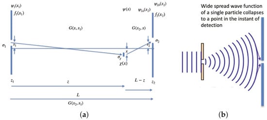
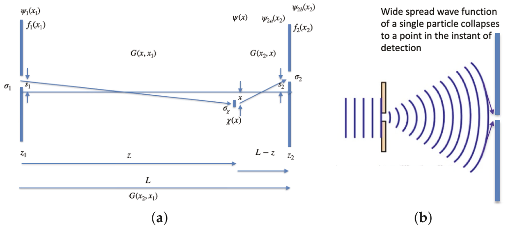
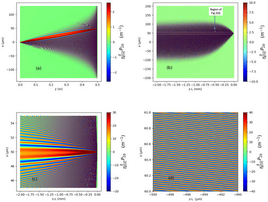
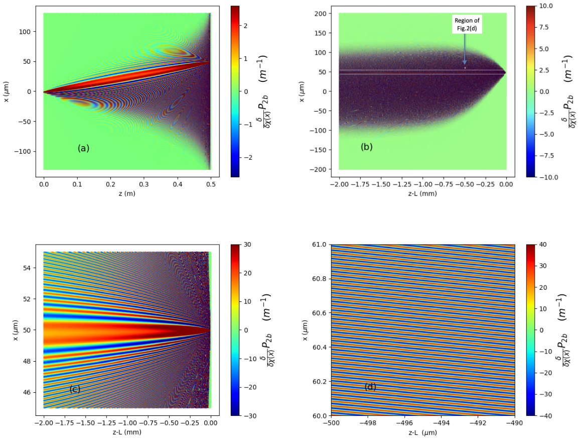
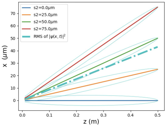
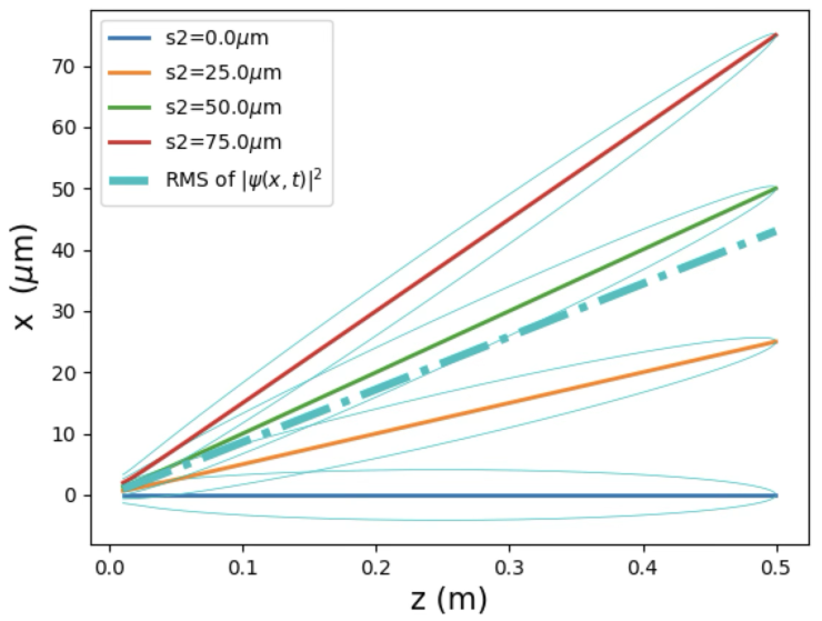
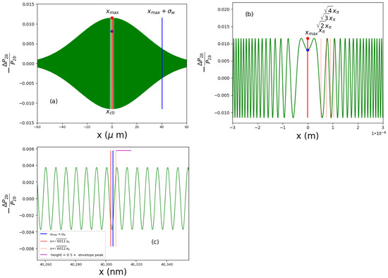
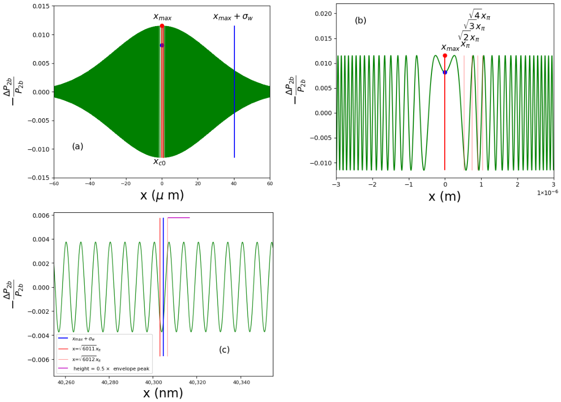
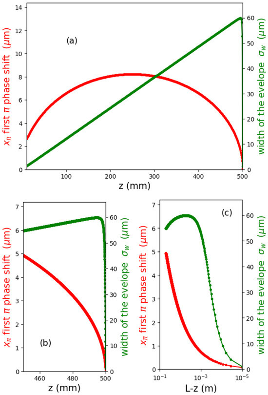
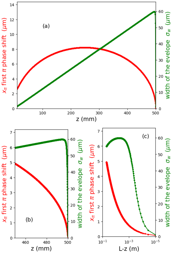
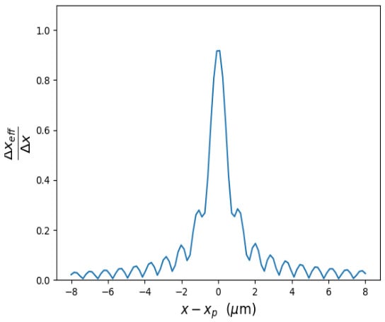
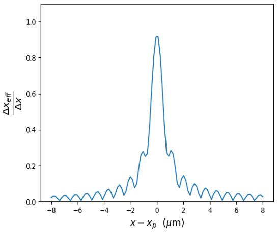
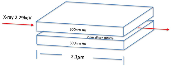
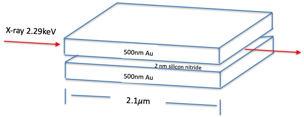
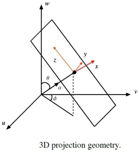
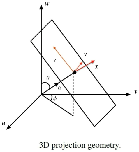
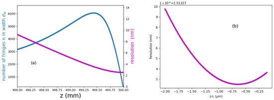
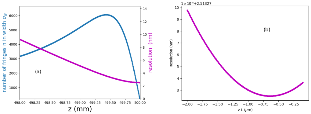
Disclaimer/Publisher’s Note: The statements, opinions and data contained in all publications are solely those of the individual author(s) and contributor(s) and not of MDPI and/or the editor(s). MDPI and/or the editor(s) disclaim responsibility for any injury to people or property resulting from any ideas, methods, instructions or products referred to in the content. |
© 2026 by the author. Licensee MDPI, Basel, Switzerland. This article is an open access article distributed under the terms and conditions of the Creative Commons Attribution (CC BY) license.