Neural Network-Driven Transmission Characteristics Modeling and Manufacturing Error Detection for Photonic Lanterns

Abstract

Traditional numerical simulation methods struggle to accurately characterize the transmission characteristics of finished photonic lanterns that contain manufacturing errors. This paper proposes a method for characterizing photonic lantern devices using neural networks. In an ideal $1\times 6$ photonic lantern, the Mean Squared Error (MSE) for predicting intensity from the multimode to the single-mode end was reduced to ${10}^{-5}$, and the neural network model can identify manufacturing error patterns, providing a new approach to addressing the precise characterization and product screening of novel irregular waveguides such as photonic lanterns.

1. Introduction

Photonics focuses on the macroscopic propagation and control of light in complex media and structures, with one of its core objectives being the realization of highly efficient, low-crosstalk multimode light field processing. Within this framework, photonic lanterns are fabricated by thermally isolating several single-mode cores within a single multimode core. They provide low-loss interfaces between single-mode and multimode systems [1]. To fully leverage the performance of photonic lanterns and guide their optimized design, precise experimental characterization and theoretical modeling of their transmission characteristics are crucial. However, manufacturing errors in photonic lanterns are difficult to measure precisely through computational simulations. Traditional physical methods—such as the Beam Propagation Method (BPM), Finite Difference Method (FDM), Eigenmode Expansion Method (EEM), or the solution of the photonic lantern transfer matrix—suffer from low simulation accuracy and are time-consuming when accounting for device manufacturing errors. In 2012, Nicolas K. Fontaine et al. at Bell Labs investigated the effects of different geometric arrangements of single-mode fiber bundles on the performance of photonic lanterns. They introduced the transfer matrix to describe the light transmission characteristics of photonic lanterns [2]. In 2014, Y. He and X. Chen pointed out that in numerical simulations, due to limited server capacity, it is impossible to include all modes in the calculations [3]. In 2019, M. Diab, S. Minardi, and colleagues demonstrated experimentally that symmetrically distributed output waveguides result in a transmission matrix with a very poor condition number, allowing only the calculation of photonic lanterns under ideal conditions [4]. In 2021, S. G. Leon-Saval and his team used a nonlinear neural network to calculate the vector transmission matrix of photonic lanterns [5]. In 2025, Wu et al. systematically modeled and optimized the transmission characteristics of photonic lanterns in the O-band to a 2 µm wavelength range by establishing a numerical model based on adiabatic conditions, with the aim of achieving efficient mode conversion over a broad bandwidth [6]. In 2026, A. K. Taras et al. demonstrated that fabrication errors cause actual devices to lose the port symmetry present in ideal models, and that the measured relative mode dispersion differs significantly from ideal predictions, strongly confirming the limitations of relying solely on ideal model-based design [7]. To achieve high-precision calibration of photonic lanterns, this paper designs a neural network model of the photonic lantern’s transmission characteristics, establishing a nonlinear mapping between the light-field data (intensity and phase) at the multimode and single-mode ends of the lantern. This approach achieves high-precision Mean Squared Error (MSE) for both ideal and manufacturing-error photonic lanterns, providing a new calibration path for optical devices such as photonic lanterns.

2. Neural Network Model of Photonic Lantern Transmission Characteristics

2.1. Photonic Lantern

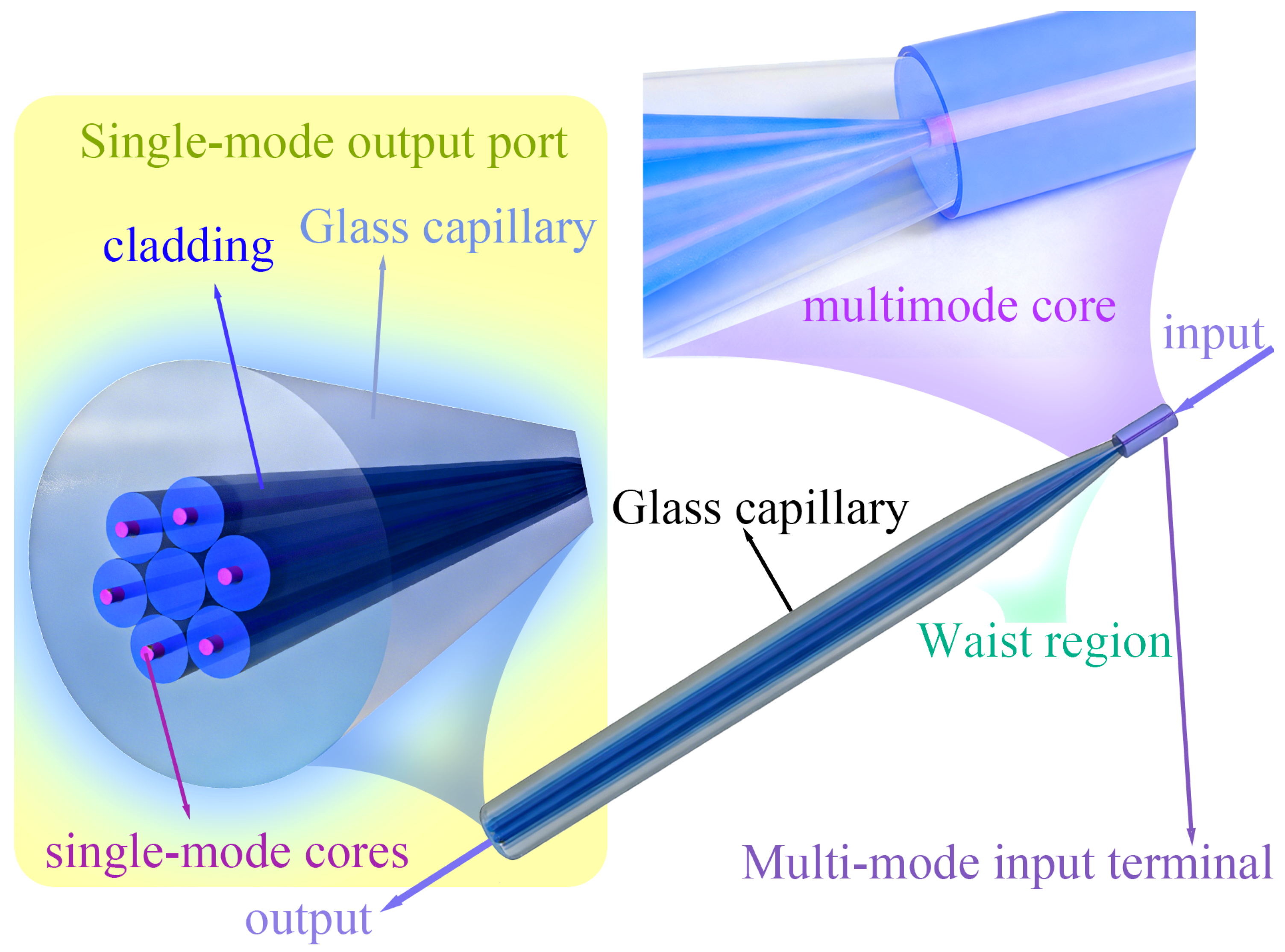
The photonic lantern is an all-fiber mode converter that enables photonics-based manipulation of light. It is a specialized waveguide structure capable of achieving low-loss, adiabatic mode evolution between a multimode waveguide and an array of single-mode fibers. The function of the photonic lantern is to linearly decompose the multimode light field information at the focal plane into a set of stable, orthogonal basis modes, which manifest at the output as the intensity and phase information detected by the single-mode fiber array, as shown in Figure 1.

As a regular optical waveguide (with a uniform longitudinal refractive index distribution), an optical fiber possesses specific boundary conditions. Under steady-state transmission conditions, a system of equations yields a finite number of discrete eigen solutions. The specific transverse light-field distribution corresponding to each eigen solution is defined as a laser transverse mode [8,9,10,11,12], hereafter uniformly abbreviated as “mode”. The main characteristics of modes are: their field distribution does not change with transmission distance; different modes within the same optical waveguide are orthogonal and can be ordered; and the total light field distribution in the fiber is a linear superposition of these modes.

Considering that common step-index fibers are circular homogeneous waveguides, the transverse distribution of the mode field is isotropic, and the refractive index varies little within each layer of the fiber (i.e., the weak-guide approximation holds), Gloge et al. proposed the scalar approximation [13], which simplifies the complex process of solving the Maxwell equations into solving the eigenvalue equations for a weak-guide step-index fiber:

$${\displaystyle \frac{U{J}_{m+1}\left(U\right)}{J_m\left(U\right)}}={\displaystyle \frac{W{K}_{m+1}\left(W\right)}{K_m\left(W\right)}}$$

(1)

where $J_m$, $K_m$ are the first-kind Bessel function and the second-kind (complex) Bessel function, respectively; U is the normalized transverse propagation constant in the core region: $U^2=\left(k_0^2{n}_1^2-{\beta }^2\right)a^2$; W is the normalized transverse attenuation function in the cladding region: $W^2=\left({\beta }^2-k_0^2{n}_2^2\right)a^2$. Here, $k_0$ is the wave number in a vacuum, $n_1$ is the refractive index of the core, $n_2$ is the refractive index of the cladding, a is the core radius, and $\beta$ is the propagation constant [14]. Defining V as the normalized frequency of the optical fiber [15]:

$$V^2=k_0^2{a}^2\left(n_1^2-n_2^2\right)={\left(k_{0}a\mathrm{NA}\right)}^2$$

(2)

it can be seen that the value of V is entirely determined by the optical fiber parameters.

The eigenvalue Equation (1) is a transcendental equation that requires numerical methods for solution. Once the geometric parameters of the fiber and the wavelength are determined, a numerical approximation of the solution can be obtained, revealing that the resulting propagation constant $\beta$ takes discrete values between $k_0{n}_2$ and $k_0{n}_1$. For each integer m, there are n solutions, corresponding to different values of ${\beta }_{mn}$, $U_{mn}$, and $W_{mn}$. A spatial field distribution determined by each set of values is called a linear polarization mode [13], denoted by $L{P}_{mn}$. Assuming the polarization direction of the incident wave is parallel to the x axis, the transverse electric field of the $L{P}_{mn}$ mode is represented by the scalar $E_x$, which is written in polar coordinates as:

$$E_x=A{e}^{i{\beta }_{mn}z}\varphi \left(m\theta \right)\left\{\begin{array}{c}{\displaystyle \frac{J_m\left(\frac{U_{mn}}{a}r\right)}{J_m\left(U_{mn}\right)}},0\le r\le a\hfill \\ {\displaystyle \frac{K_m\left(\frac{W_{mn}}{a}r\right)}{K_m\left(W_{mn}\right)}},r>a\hfill \end{array}\right.$$

(3)

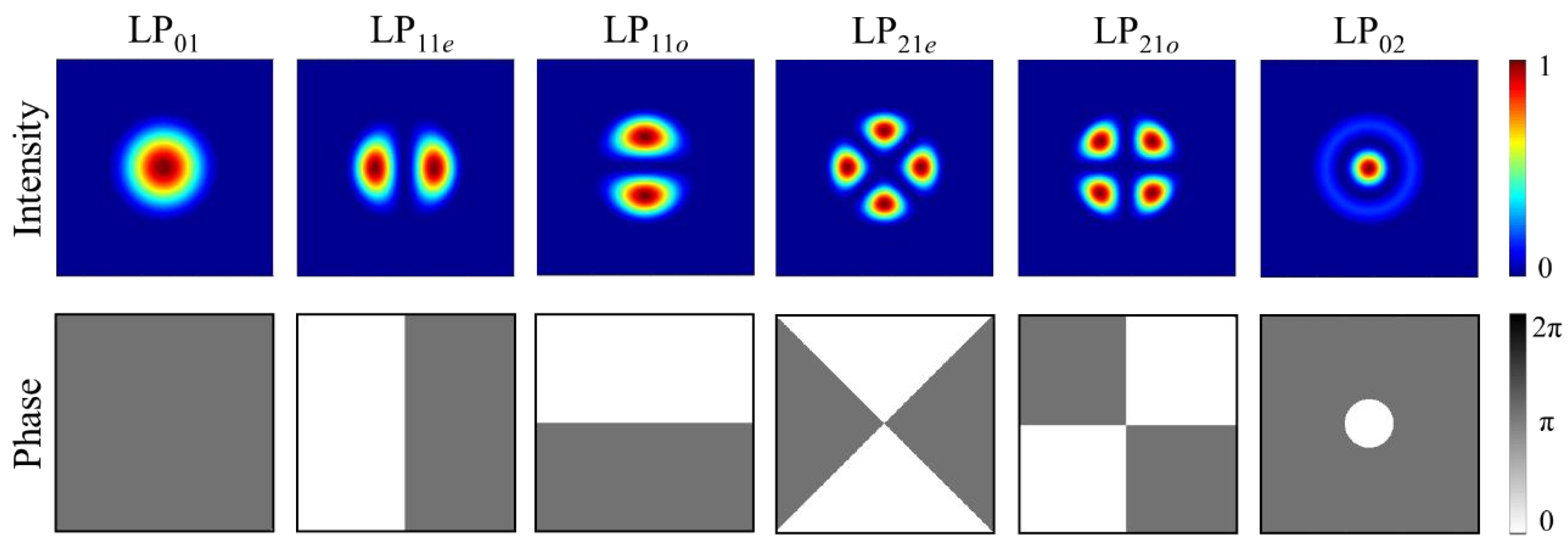
where $\varphi \left(m\theta \right)$ reflects the angular distribution of the light field. When $m>0$, $\varphi \left(m\theta \right)$ can take the form of $\cos \left(m\theta \right)$ or $\sin \left(m\theta \right)$, representing the two degenerate states of the $L{P}_{mn}$ mode: the “even” mode and the “odd” mode, distinguished by the subscripts $L{P}_{mne}$ and $L{P}_{mno}$. Figure 2 shows schematic diagrams of the near-field intensity and phase distributions for six typical $LP$ modes in a step-index fiber. A $1\times 6$ photonic lantern has exactly six modes, and the optical field information—including both intensity and phase—is input at the multimode end of the photonic lantern.

Numerical simulations of the evolution of a $1\times 6$ photonic lantern have revealed a one-to-one correspondence between the input and output light fields of the photonic lantern. Drawing on the concept of the transmission matrix [16,17], this relationship between the input and output light fields of the photonic lantern can be concisely expressed as:

$$u=M·v$$

(4)

where M is the transmission matrix of the photonic lantern, v is a column vector describing the optical field information at the single-mode end of the photonic lantern, $v^T=\left[v_1{e}^{j{\theta }_1},v_2{e}^{j{\theta }_2},v_3{e}^{j{\theta }_3}\right]$ (where $v_i$ and ${\theta }_i$ denote the amplitude and phase, respectively, of the fundamental mode optical field input from the i single-mode fiber), u is the column vector describing the optical field information at the multimode end of the photonic lantern, $u^T=\left[u_1{e}^{j{\varphi }_1},u_2{e}^{j{\varphi }_2},u_3{e}^{j{\varphi }_3}\right]$ (where $u_i$ and ${\varphi }_i$ denote the amplitude and phase of the i eigenmode in the output superposition field, respectively).

The physical structure of the photonic lantern exhibits inherent regularities, and its transmission characteristics can be expressed using nonlinear functions. Deep learning possesses strong capabilities for handling nonlinear problems and can approximate highly nonlinear functions with fewer parameters.

2.2. Neural Networks

A neural network is a computational model that mimics the connections between neurons in the human brain. It approximates complex functions by constructing multiple layers of nonlinear transformations. Its core lies in introducing nonlinear activation functions (LeakyReLU is used in this paper) to transform linear combinations into nonlinear mappings. The General Approximation Theorem states that, provided the hidden layer is sufficiently wide, this structure can approximate any continuous function on a compact domain with arbitrary precision, laying the theoretical foundation for neural networks to handle nonlinear regression problems [18].

From a mathematical perspective, the propagation process of a photonic lantern can be represented as a nonlinear operator T, which maps the input light field $I_{\mathrm{in}}$ into the output light field $I_{\mathrm{out}}$:

$$I_{\mathrm{out}}=T\left(I_{\mathrm{in}},\lambda \right)$$

(5)

where $\lambda$ represents parameters such as wavelength. Neural networks can leverage their nonlinear mapping capabilities to learn an approximate representation of this operator. Through multiple layers of nonlinear transformations, any continuous function can be approximated, providing a mathematical guarantee of accurate modeling of the photonic lantern’s transmission characteristics.

From a physical perspective, the photonic lantern is a multi-input, multi-output optical device whose transmission characteristics follow the laws of electromagnetic wave propagation described by Maxwell’s equations. Although the underlying physical mechanisms are complex, this process is essentially a deterministic mapping: given specific input light-field parameters, a corresponding output light-field distribution is generated. Therefore, it can be abstracted as a deterministic nonlinear system, and neural networks are particularly adept at learning such complex input-output mapping relationships.

Consequently, if there exists an intrinsic, continuous functional relationship between the transmission characteristics of the photonic lantern and its input parameters, and if we can obtain a sufficiently large dataset that is well-distributed across the input parameter space, features high data quality, and has accurate labels, while simultaneously selecting an appropriate neural network architecture and conducting effective training (including measures to prevent overfitting), then the neural network has the potential to learn and establish a high-precision regression model for the transmission characteristics of the photonic lantern.

In regression tasks, the learning process is driven by minimizing a loss function (such as the MSE, used in this paper). Given the training data $(x_i,y_i)$, the training objective is to minimize the loss function $L\left(\theta \right)$, as shown in Equation (6):

$$L\left(\theta \right)={\displaystyle \frac{1}{N}}{\displaystyle \sum _{i=1}^N}{\left(y_i-f(x_i,\theta )\right)}^2$$

(6)

The core parameters are optimized using gradient descent, and the update rule is given by Equation (7):

$${\theta }^{(t+1)}={\theta }^{\left(t\right)}-\eta {\nabla }_{\theta }L\left({\theta }^{\left(t\right)}\right)$$

(7)

where $\eta$ is the learning rate. Gradient calculation relies on the backpropagation algorithm, which uses the chain rule to propagate the output error backward through each layer to the respective parameters, efficiently computing the gradient [19].

To prevent overfitting and improve generalization ability, regularization techniques are commonly employed. For instance, this paper uses Dropout regularization, which randomly deactivates a portion of neurons during training, to reduce cooperative adaptation among neurons. This enables the network to learn feature representations with greater redundancy and generalization, thereby enhancing the model’s robustness. Additionally, this paper employs techniques such as learning rate decay to effectively regulate the training process. When training stalls, the search step size is adaptively refined, effectively balancing global optimization efficiency with local convergence accuracy to suppress overfitting and ensure the model possesses good generalizability.

3. Method

3.1. Light Field Dataset

Based on numerical simulations of traditional light-beam propagation algorithms (RSoft BeamPROP, BPM algorithm), this paper designs and implements a $1\times 6$ photonic lantern for experiments, collecting large amounts of input light-field data (optical power and phase) and output light-field data (optical intensity and phase). This data is used to construct a light field dataset based on the physical principles of photonic lantern mode evolution.

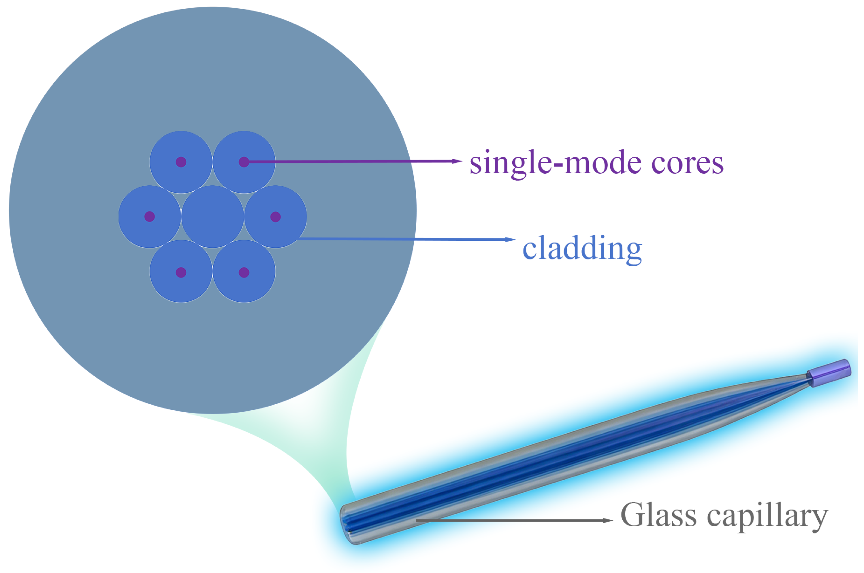
The structure of the $1\times 6$ photonic lantern described in this paper employs an adiabatic taper-coupling design between a multimode fiber (MMF) and a single-mode fiber array (SMF array). The core diameter is $10.0\mathsf{\mu }\mathrm{m}$, the cladding diameter is $125.0\mathsf{\mu }\mathrm{m}$, and the taper ratio is 13.25. The operating wavelength is $1.064\mathsf{\mu }\mathrm{m}$, the cladding refractive index is 1.435, and the refractive index difference is 0.01, meaning the core refractive index is 1.445. The numerical simulations were performed using RSoft BeamPROP with the following parameters: grid resolution of $0.8\mathsf{\mu }\mathrm{m}$ in the X and Y directions (cross-section of the photonic lantern) and $2\mathsf{\mu }\mathrm{m}$ in the Z direction (propagation direction); the simulation domain is a rectangular prism with a base side of $300\mathsf{\mu }\mathrm{m}$ and a height of $\mathrm{26,800}\mathsf{\mu }\mathrm{m}$, centered at the $1\times 6$ multimode port of the photonic lantern; the propagation step size is set to $2\mathsf{\mu }\mathrm{m}$, consistent with the Z-axis resolution, and verification at $\mathrm{13,400}\mathsf{\mu }\mathrm{m}$ confirmed the accuracy of the simulation. As shown in Figure 3, the input light field at the multimode end of the photonic lantern consists of a linear superposition of six orthogonal ${\mathrm{LP}}_{\mathrm{mn}}$ modes. Each data set consists of randomly generated optical powers ([0–1]) and phase differences (in degrees, [0–360]) for the six fundamental modes. A total of N sets of input light field data are generated and saved as a .txt file. Through simulation, following a fixed order, the 6 pairs of average light intensities and phase differences (in degrees, [0–360]) detected at the 6 single-mode ports are recorded, yielding N sets of output light-field data, which are saved as text files. Each set of input light field data corresponds to a set of output light field data, forming a data pair, yielding a total of N pairs. The input and output light field data together form the input light field dataset. To optimize the neural network, the light-field data is normalized during training.

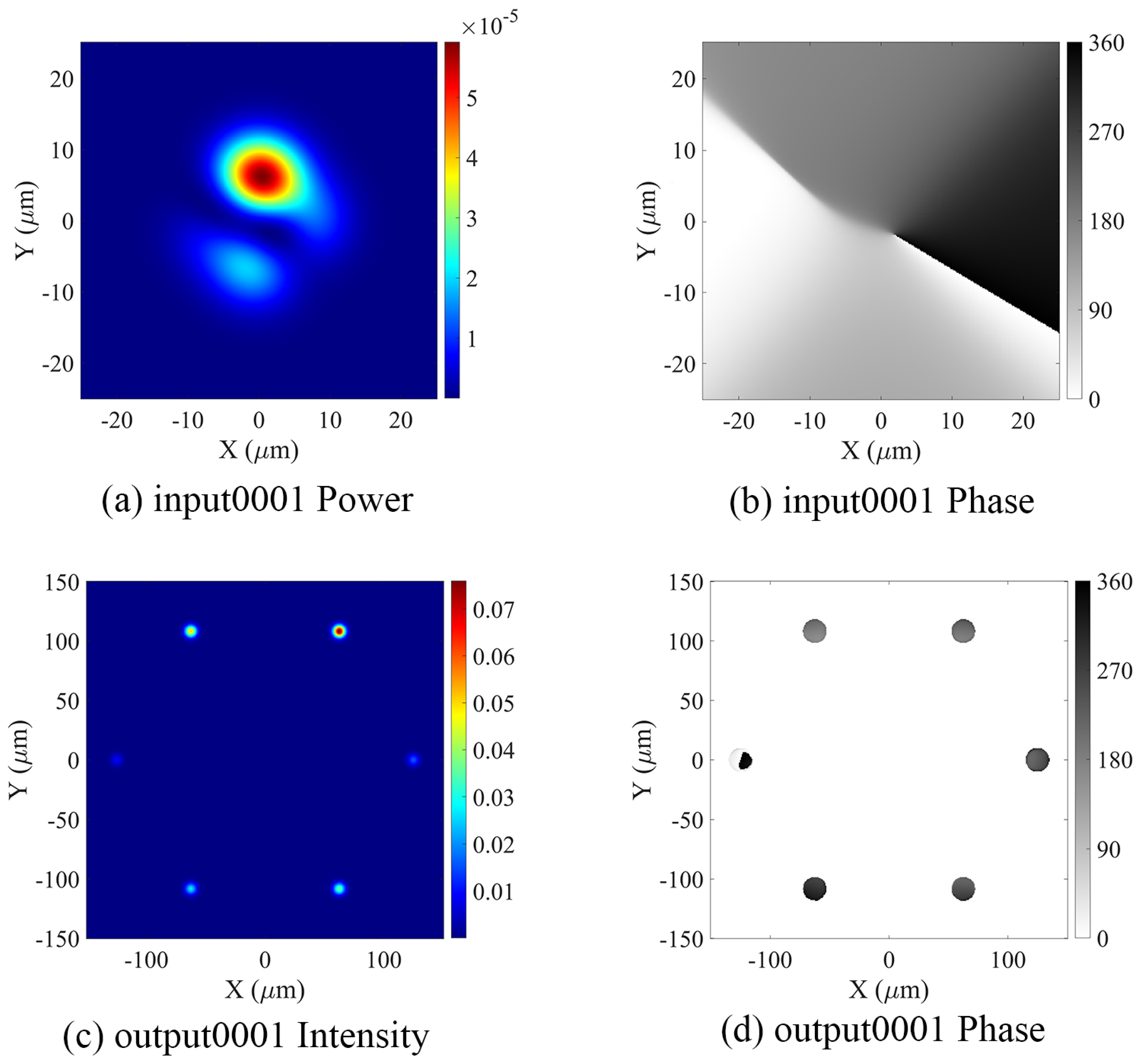
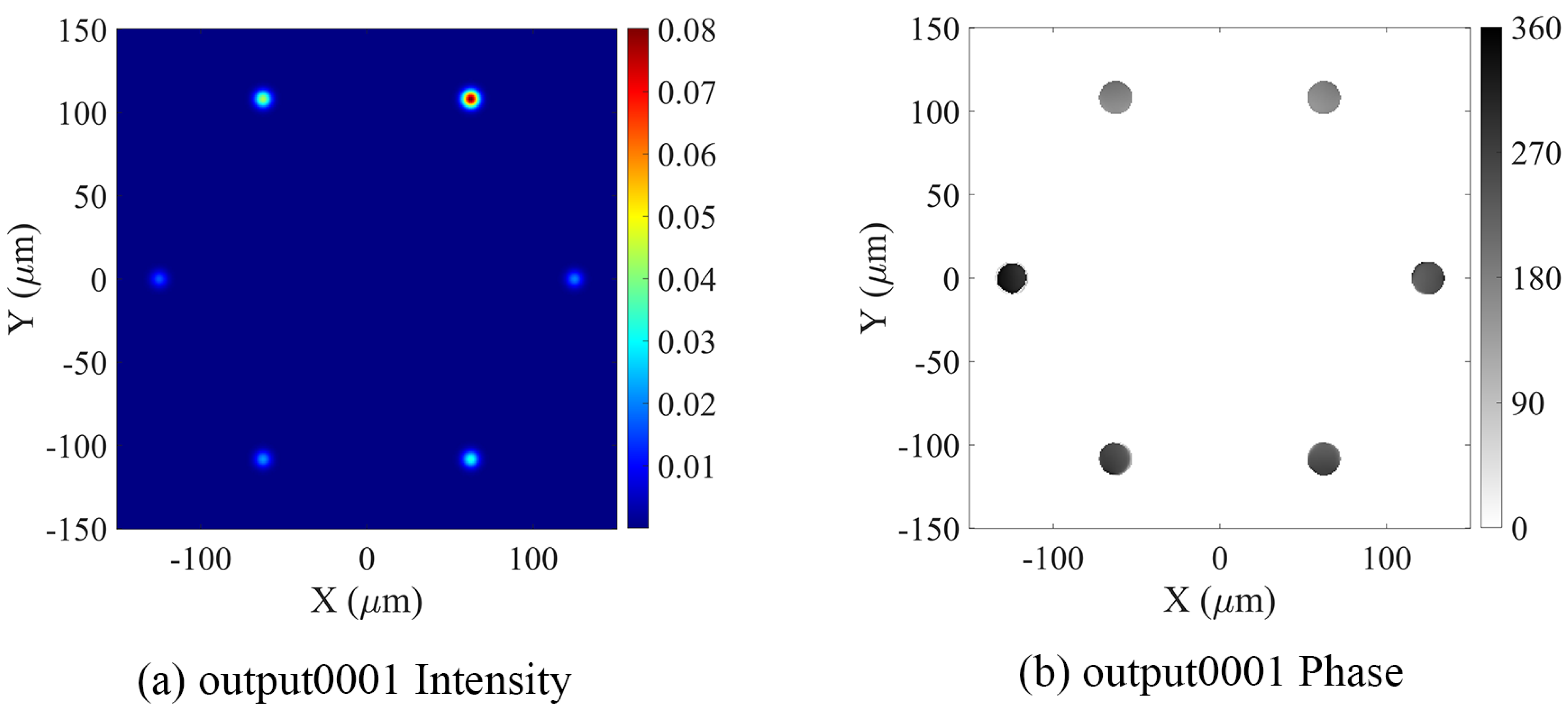
As shown in

Table 1. Examples of Light Field Datasets.

Filename	Context
input0001	0.14 191 0.18 276 0.40 221 0.23 336 0.03 282 0.02 272
output0001	0.009012 6.1054 0.050812 186.04 0.02652 294.62 0.035892 245.89 0.076959 205.17 0.015572 241.77

, input and output data with the same numerical suffix correspond one to one. For example, Figure 4 shows the intensity and phase images for the input light field at the multimode end and the output at the single-mode end of an ideal $1\times 6$ photonic lantern.

This paper presents experiments using five model types: an ideal $1\times 6$ photonic lantern, a $1\times 6$ photonic lantern with misaligned fusion joints (two misalignment scenarios), and a $1\times 6$ photonic lantern with non-uniform taper (non-uniform fiber volume and non-uniform arrangement).

3.1.1. Ideal $1\times 6$ Photonic Lantern

An ideal photonic lantern enables low-loss, low-mode-dependent coupling between multiple single-mode fibers (SMFs) and a single multimode fiber (MMF) [1].

In an ideal photonic lantern, since the six input fundamental modes and the six single-mode fibers exhibit both vertical and horizontal symmetry, the data for the ideal $1\times 6$ photonic lantern was expanded using vertical flipping and horizontal mirroring methods. As shown in Figure 2 above, based on the phase-symmetry relationships among the six fundamental modes, the light field dataset is expanded to 4 times the original number of light field data pairs, yielding $4N$ sets of light field data pairs. Specifically, ${\mathrm{LP}}_{01}$, ${\mathrm{LP}}_{11\mathit{e}}$, ${\mathrm{LP}}_{11\mathit{o}}$, ${\mathrm{LP}}_{21\mathit{e}}$, ${\mathrm{LP}}_{21\mathit{o}}$, and ${\mathrm{LP}}_{02}$ correspond sequentially to the input light field data at the multimode end, while the single-mode fibers numbered 1 through 6 (from left to right and top to bottom) correspond to the output light field data. The phase distributions of ${\mathrm{LP}}_{01}$ and ${\mathrm{LP}}_{02}$ are fully symmetric and do not affect the phase evolution, whereas ${\mathrm{LP}}_{11\mathit{e}}$, ${\mathrm{LP}}_{11\mathit{o}}$, ${\mathrm{LP}}_{21\mathit{e}}$, and ${\mathrm{LP}}_{21\mathit{o}}$ exhibit phase symmetry. When the phase of ${\mathrm{LP}}_{11\mathit{o}}$ and ${\mathrm{LP}}_{21\mathit{o}}$ is increased by ${180}^{\circ }$, the phase at single-mode outputs 3 and 4 increases by ${180}^{\circ }$; when the phase of ${\mathrm{LP}}_{11\mathit{e}}$ and ${\mathrm{LP}}_{21\mathit{o}}$ is increased by ${180}^{\circ }$, the phase at outputs 1, 2, and 3 increases by ${180}^{\circ }$; when the phase of ${\mathrm{LP}}_{11\mathit{e}}$, ${\mathrm{LP}}_{11\mathit{o}}$, and ${\mathrm{LP}}_{21\mathit{o}}$ is increased by ${180}^{\circ }$, the phase at outputs 1, 2, 3, 4, and 6 increases by ${180}^{\circ }$. Based on this principle, each original input-output pair is quadrupled: the first pair is an exact copy; the second pair increases the phase of the 3rd and 5th input modes by ${180}^{\circ }$ and the 3rd and 4th output ports by ${180}^{\circ }$; the third pair increases the phase of the 2nd, 3rd, and 5th input modes by ${180}^{\circ }$ and the 1st, 2nd, 3rd, 4th, and 6th output ports by ${180}^{\circ }$. All phase values are kept within 0–${360}^{\circ }$ via modulo operation.

3.1.2. Lateral-Offset Splicing

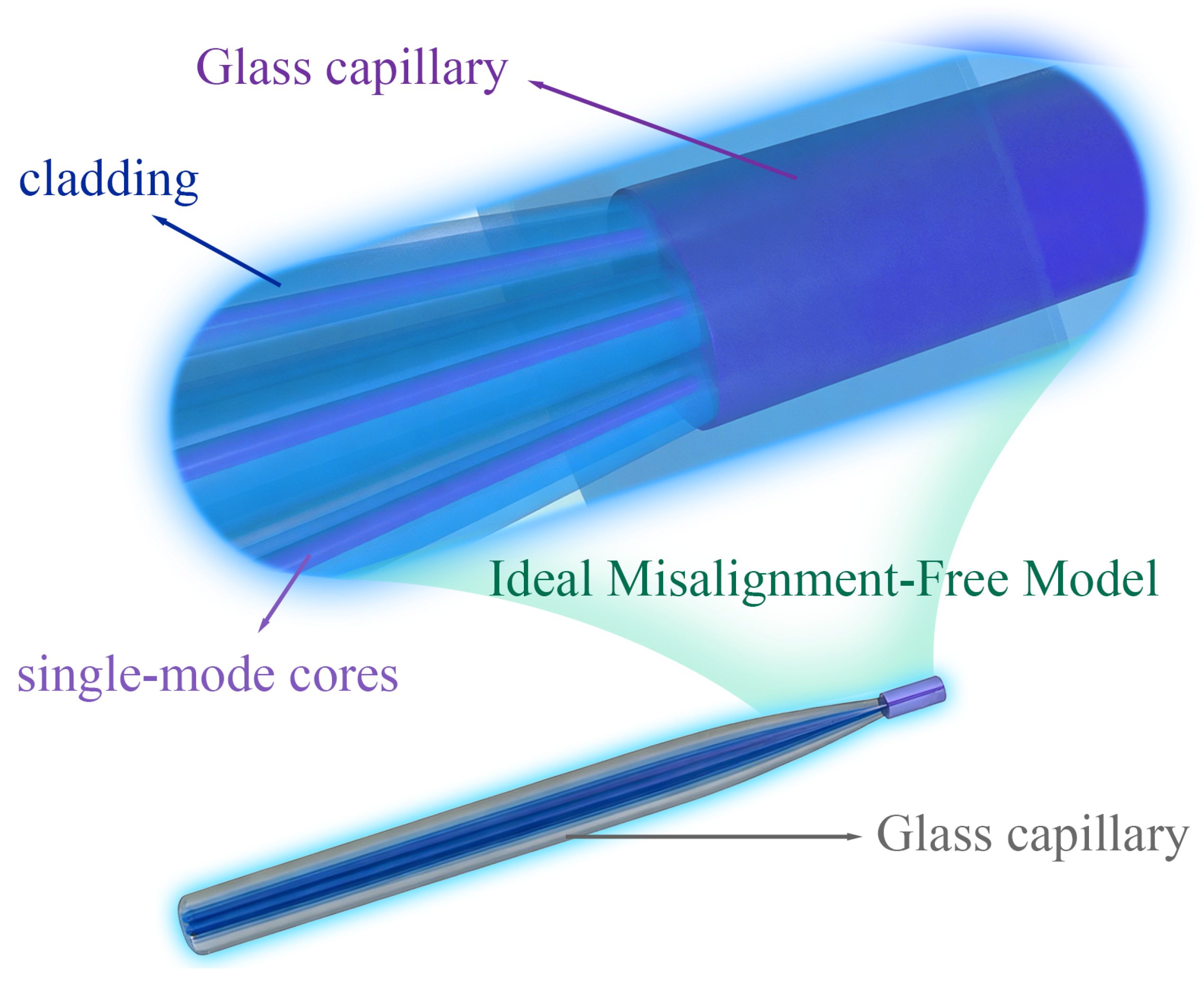
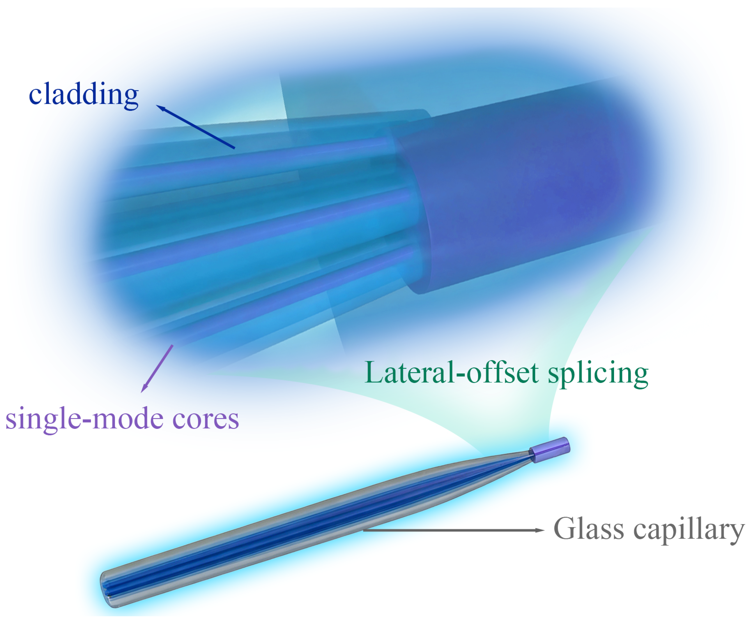
As compared in Figure 5 and Figure 6 below, lateral-offset splicing is a common and significant process defect in the manufacture of photonic lanterns, particularly when connecting single-mode fiber bundles to multimode fiber. This manufacturing error directly disrupts the ideal alignment of the optical path. It destroys the central symmetry of the light field, leading to unexpected coupling as the fundamental mode evolves into higher-order modes, thereby increasing insertion loss and being one of the primary sources of optical loss. Optical loss increases nonlinearly with increasing offset distance [20].

In this paper, the end face of the waist region of the single-mode fiber was shifted relative to the matched multimode fiber during splicing, i.e., the entire structure was offset from the ideal optical axis, to simulate misaligned splicing. Two sets of optical field datasets (Unidirectional offset and Bidirectional offset) were obtained through simulation, with parameter configurations shown in

Table 2. Parameters of the Offset Fusion Photonic Lantern Model.

Type	X Offset	Y Offset
Unidirectional offset	$4\mathsf{\mu }\mathrm{m}$	$0\mathsf{\mu }\mathrm{m}$
Bidirectional offset	$-4\mathsf{\mu }\mathrm{m}$	$4\mathsf{\mu }\mathrm{m}$

.

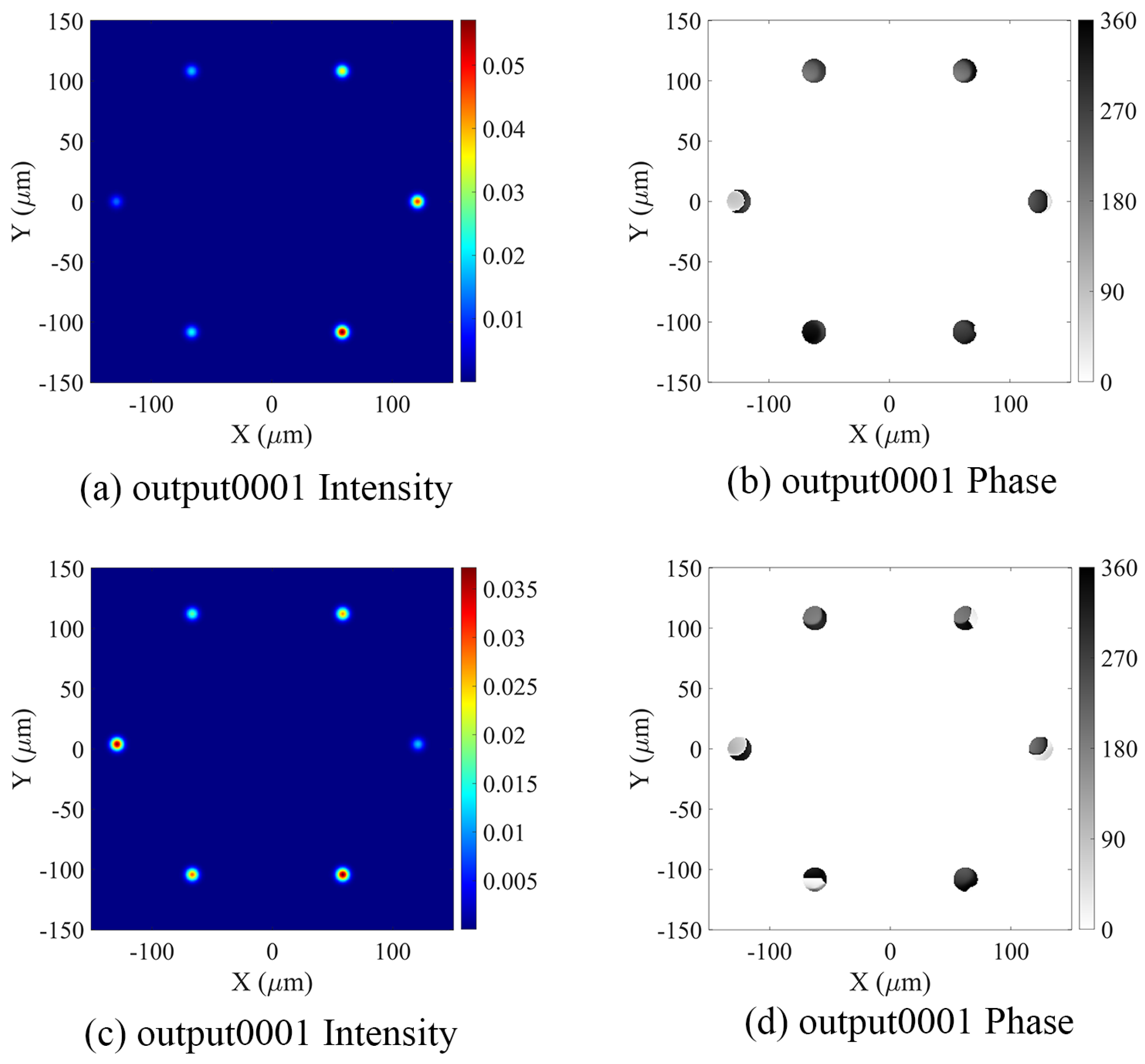
Since misaligned welding disrupts symmetry, the light field dataset here does not use symmetrically augmented data; instead, all training is performed using the original data. The following Figure 7, Figure 8 and Figure 9 show the example of lateral-offset splicing light field data.

3.1.3. Non-Uniform Tapering

Taper is a core process in the fabrication of photonic lanterns. It involves heating and stretching a fiber bundle to gradually reduce its cross-sectional dimensions, thereby achieving adiabatic mode evolution. The uniformity of the tapering process, particularly heating, is critical to the device’s final performance [21]. Non-uniform tapering primarily results from non-uniform distribution of the tensile force during electrode discharge, leading to non-uniform heating, as well as non-uniform internal arrangement of the fiber bundle.

Non-Uniform Heating

Photonic lanterns are typically manufactured using an optical fiber tapering process, which is extremely sensitive to the stability, shape, and position of the heat source (such as a flame) [20]. Flames are prone to turbulence and can fluctuate easily due to slight variations in airflow or residual air currents within the chamber; impure gases may also lead to fiber contamination [22]. A non-uniform static heat source typically produces a non-uniform taper waist diameter, leading to variations in the taper ratio across cores and disrupting phase-matching conditions between channels. This means that the cross-sectional dimensions of the taper zone vary along its length, and such variations can only be predicted through experimental calibration; they are difficult to control precisely using theoretical models [21].

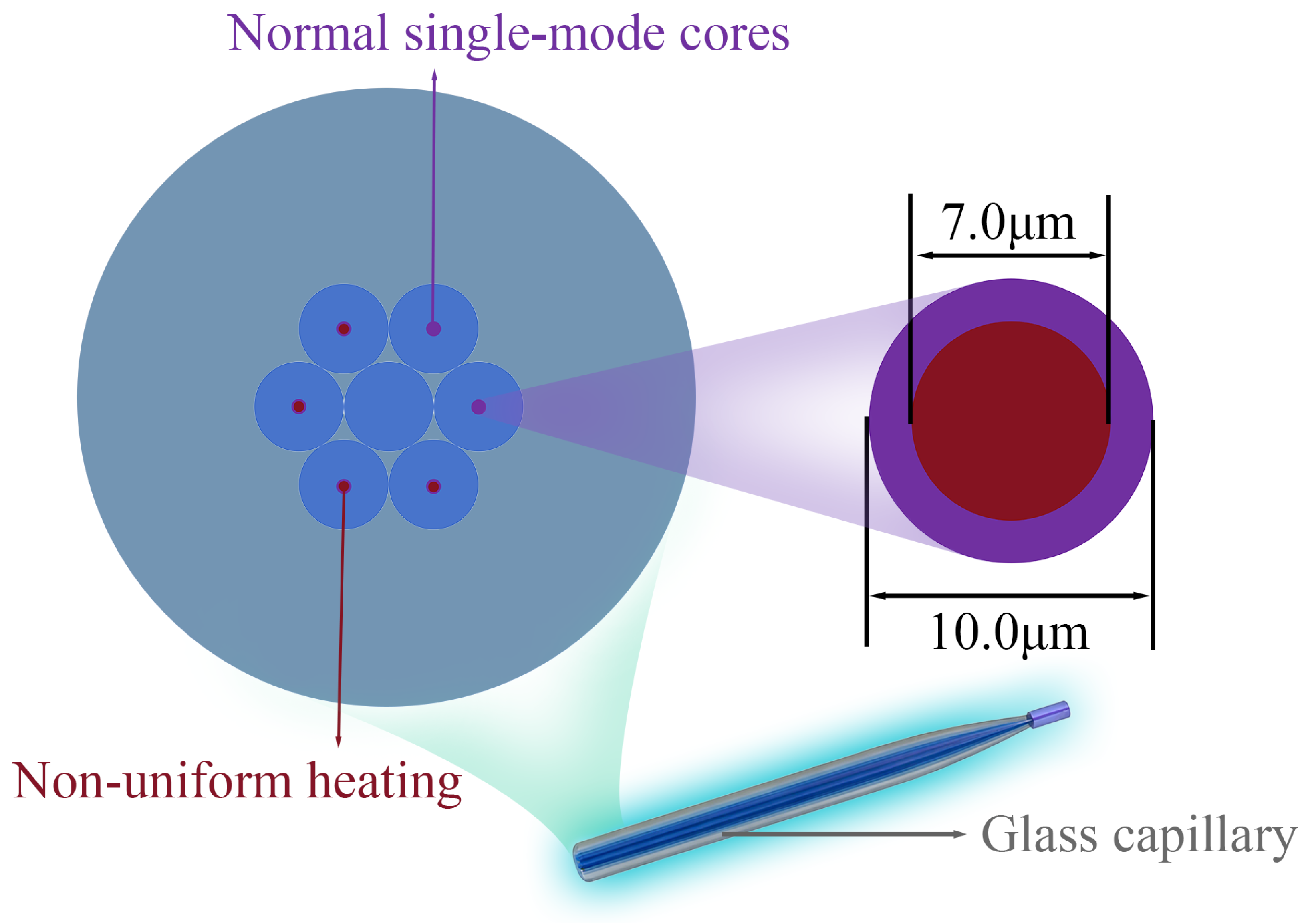
As an example in Figure 10, errors caused by non-uniform heating reduced the coordinates and dimensions of certain core segments in four single-mode fibers within a $1\times 6$ photonic lantern by $30\%$, resulting in these fibers being drawn thinner. Since non-uniform heating disrupts the symmetry of the photonic lantern, the light-field dataset here does not use symmetry-augmented data; instead, all training is performed on raw data. Example of light field data is shown in Figure 11 and Figure 12.

Non-Uniform Arrangement

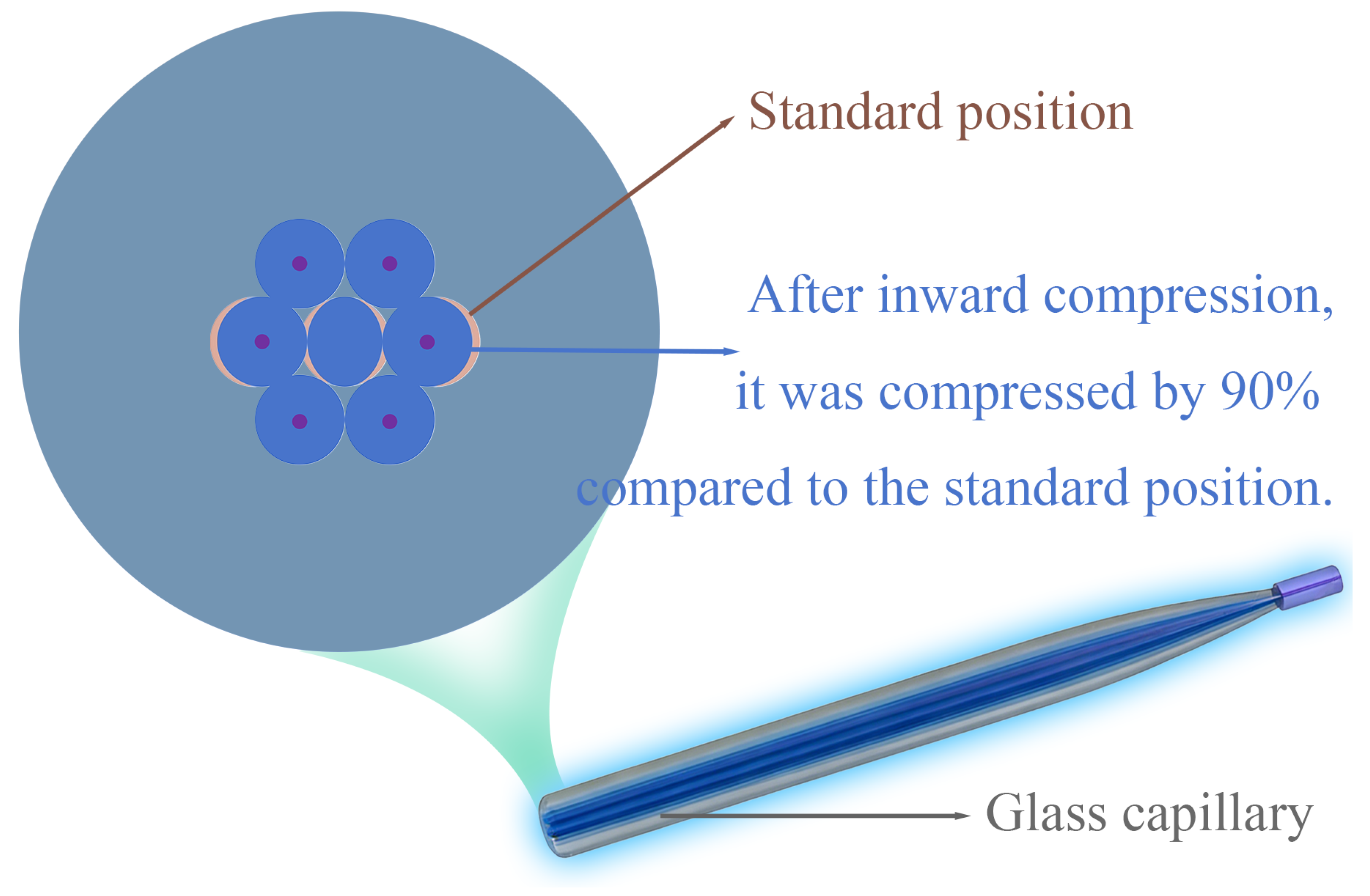
Ideally, the geometric arrangement of the cores should match the symmetry of the photonic lantern mode to minimize mode-dependent loss [23]. However, when bundling multiple single-mode fibers, if the core arrangement does not conform to the ideal geometric symmetry (e.g., a tight hexagonal arrangement) or if the core spacing is inconsistent, then during the drawing process, even with uniform heating, differences in the evolution paths and mutual coupling strengths of different cores will arise, equivalent to a form of structural non-uniformity. This model simulates the geometric positional deviations caused by loose fiber packing within the capillary.

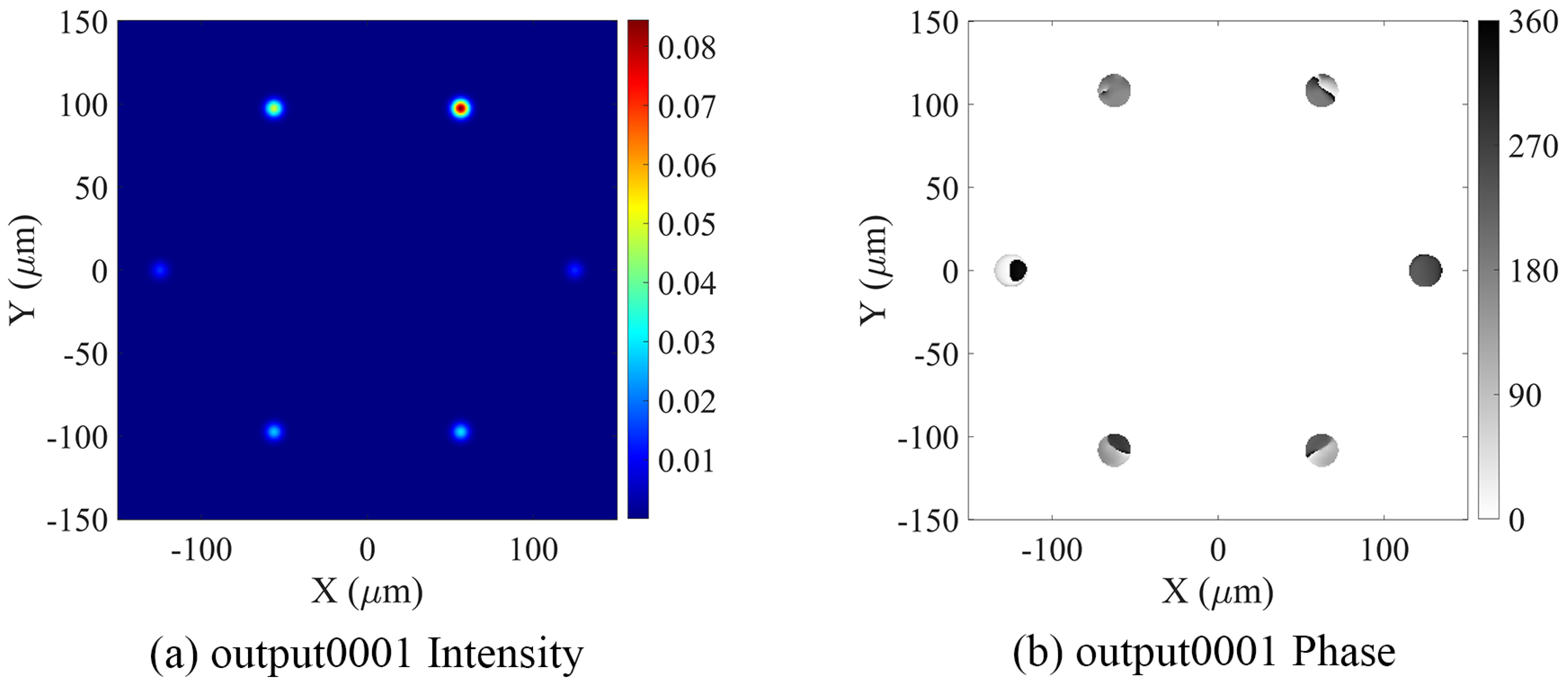
In a non-uniform arrangement shown in Figure 13, two symmetrically positioned cores are shifted inward by $10\%$, compressing the fiber arrangement and disrupting the ideal hexagonal close-packed structure. Example of light field data is shown in Figure 14 and Figure 15.

3.2. Designing Neural Networks for Light Field Data Based on Light Field Datasets

This paper designs neural networks with different parameter settings based on a light-field dataset ($N>1000$). The dataset is divided into training, validation, and test sets, ensuring that the validation and test sets are drawn from the original dataset, with a 90:5:5 split.

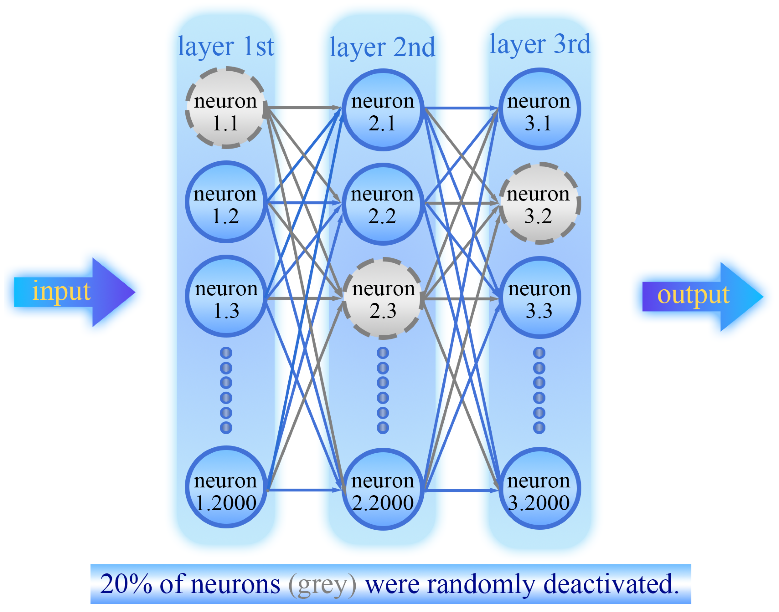
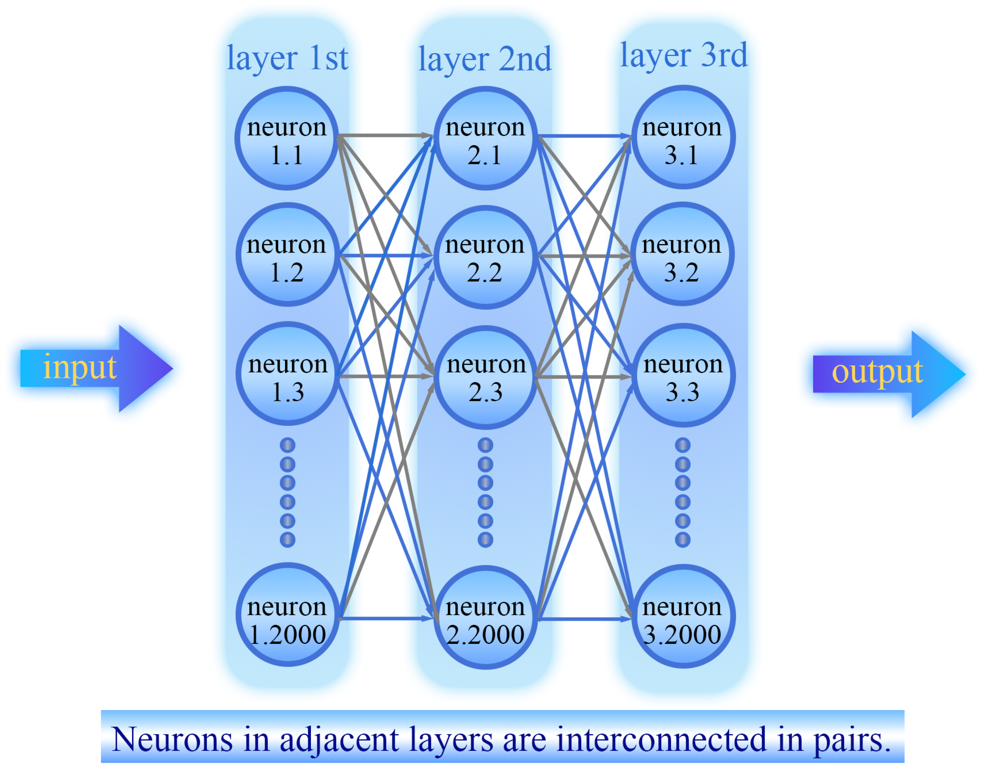
This paper adopts a Dropout network. A Dropout network is a model that systematically and strategically applies dropout or its variants within a deep neural network architecture. During the training phase, it uses a probability p as a hyperparameter to randomly remove neurons and their connections from the network for regularization, thereby preventing excessive co-adaptation among neurons and effectively mitigating overfitting [24]. For example, if the hyperparameter p is set to 0.2, each neuron has a $20\%$ probability of being set to zero during each forward pass. Figure 16 and Figure 17 illustrate a 3-layer Dropout network.

Derivation shows that for the activation output of layer l ($a^{\left(l\right)}$), during training, an element-wise multiplication is performed with a mask vector $m^{\left(l\right)}$, where the elements of $m^{\left(l\right)}$ are independently set to 0 with probability p and to 1 with probability $1-p$, i.e., ${\tilde{a}}^{\left(l\right)}=a^{\left(l\right)}\odot m^{\left(l\right)}$, to perform random dropout.

Additionally, to avoid the need for random dropout during the testing phase while maintaining the expected value of the output, the retained activation values are scaled during training, i.e., ${\tilde{a}}^{\left(l\right)}={\displaystyle \frac{1}{1-p}}(a^{\left(l\right)}\odot m^{\left(l\right)})$, which is referred to as Inverted Dropout.

Here, ⊙ is an operator that performs element-wise multiplication followed by division by $1-p$, ensuring that the expected values remain consistent between the training and testing phases.

In this paper, the model uses the MSE as the loss function to quantify the difference between the predicted light intensity and phase at the output and the true values. The MSE and the coefficient of determination $R^2$ are used to evaluate the performance of the regression model. The optimal model is obtained through parameter tuning.

The dropout mechanism involves applying a random mask $m^{\left(l\right)}$ to the activation vector $a^{\left[l\right]}$ during the forward pass at layer l (where each element takes the value 0 with probability p and the value 1 with probability $1-p$), resulting in:

$${\tilde{a}}^{\left(l\right)}={\displaystyle \frac{1}{1-p}}\left(m^{\left(l\right)}\odot a^{\left(l\right)}\right)$$

(8)

During testing, $m^{\left(l\right)}\equiv 1$ and the full $a^{\left[l\right]}$ is used directly.

For the light field intensity prediction task, let the network output be ${\widehat{I}}_{\mathrm{out}}=f_{\theta }\left(I_{\mathrm{in}}\right)$ and the true light field be $I_{\mathrm{out}}$. The MSE loss is defined as:

$$L_{\mathrm{MSE}}\left(\theta \right)={\displaystyle \frac{1}{N}}{\displaystyle \sum _{i=1}^N}{\parallel {\widehat{I}}_{\mathrm{out}}^{\left(i\right)}-I_{\mathrm{out}}^{\left(i\right)}\parallel }_2^2$$

(9)

where N is the number of training samples.

After introducing dropout into each layer of the network, the overall objective remains to minimize MSE, but gradients are computed based on the “sparse” subnetworks at each iteration, thereby suppressing feature co-adaptation and improving generalization. The complete optimization problem can be written as:

$$\underset{\theta }{\min }{E}_{m^{\left[l\right]}}\left[{\displaystyle \frac{1}{N}}{\displaystyle \sum _{i=1}^N}{\parallel f_{\theta }^{\mathrm{drop}}\left(I_{\mathrm{in}}^{\left(i\right)}\right)-I_{\mathrm{out}}^{\left(i\right)}\parallel }_2^2\right]$$

(10)

where $f_{\theta }^{\mathrm{drop}}$ denotes the network with the dropout mask applied to the layer during forward propagation [25].

The network architecture in this paper employs LeakyReLU as the activation function across all layers, with a hyperparameter of 0.3, which is well-suited for continuous regression tasks in modeling the transmission characteristics of photonic lanterns. The Dropout design follows three principles: all hidden layers use the same Dropout rate to ensure consistent regularization effects; Dropout is applied after LeakyReLU to randomly deactivate activation values, thereby enhancing model robustness; the output layer does not use Dropout to ensure deterministic prediction results. Preliminary experiments show that setting the Dropout rate to 0.2 yields the lowest MSE on the validation set and relatively stronger generalization ability. With the Dropout rate kept constant, experiments were conducted with varying numbers of layers to identify the neural network model that achieves the best MSE on the validation set.

4. Results and Discussion

4.1. Performance of the Ideal Optical Sub-Lantern Transmission Characteristics Neural Network Model

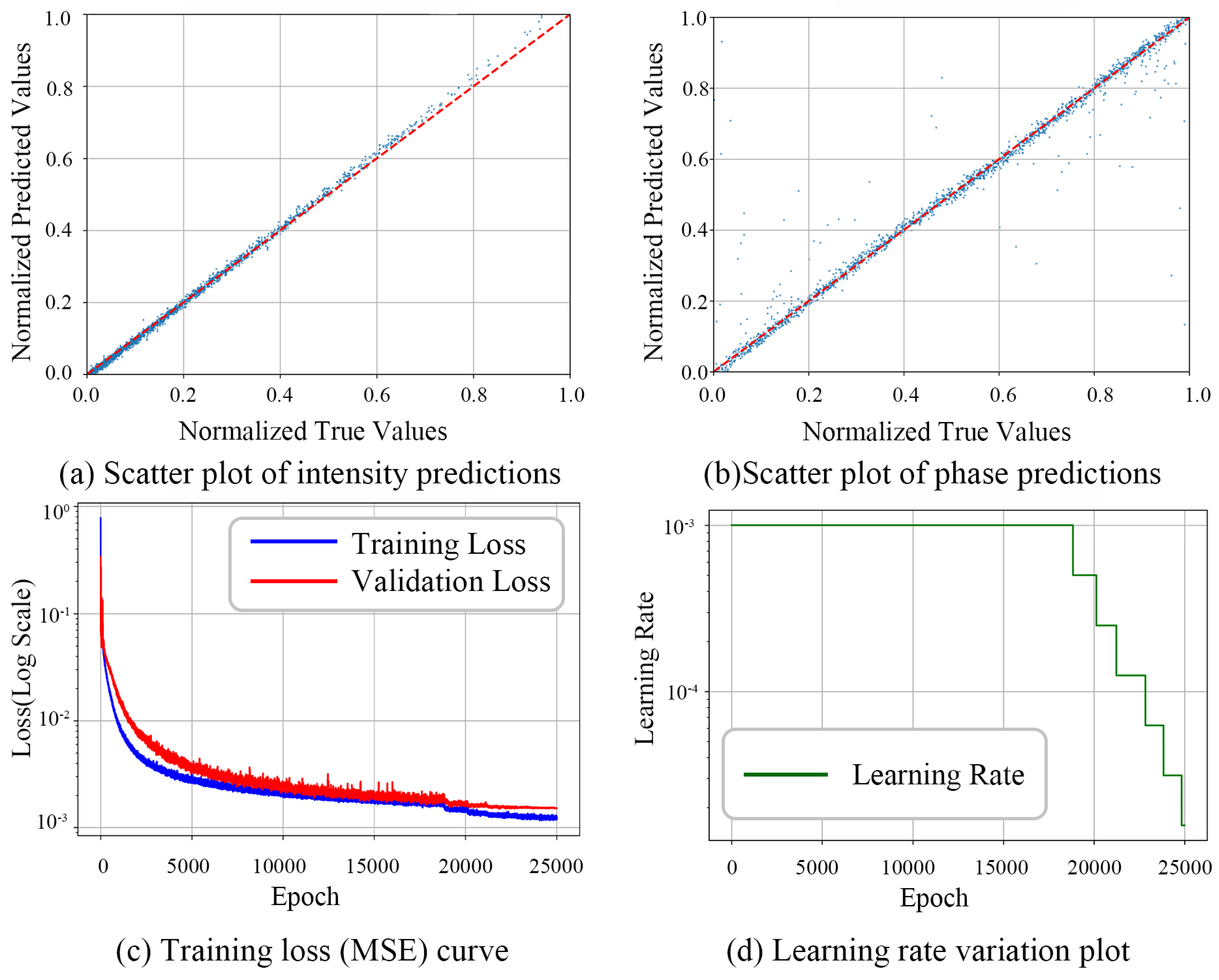
This paper constructs a Dropout Network using dropout regularization, with all hyperparameters set to 0.2, meaning that in each training iteration, each neuron has a $20\%$ probability of being dropped. The training batch size is set to 64, and the training runs 25,000 iterations. A strategy dynamically adjusts the learning rate; the system continuously monitors the validation set loss. If the improvement in the loss is less than ${10}^{-6}$ over 1000 consecutive iterations, the learning rate is reduced to $50\%$ of its current value, with a lower limit set at $5\times {10}^{-7}$.

Table 3. Performance Summary of the Dropout-Based Ideal Photonic Lantern Transmission Characteristics Neural Network.

Layers	Hidden Layer Size	Training Examples	Intensity MSE (Norm. Units)	Intensity R2 (Norm. Units)	Phase MSE (Norm. Units)	Phase R2 (Norm. Units)
3	2000	6000(1500)	$9.793\times {10}^{-5}$	$9.973\times {10}^{-1}$	$4.063\times {10}^{-3}$	$9.516\times {10}^{-1}$
5	2000	6000(1500)	$1.167\times {10}^{-4}$	$9.967\times {10}^{-1}$	$3.814\times {10}^{-3}$	$9.546\times {10}^{-1}$
9	2000	6000(1500)	$1.196\times {10}^{-4}$	$9.967\times {10}^{-1}$	$4.529\times {10}^{-3}$	$9.461\times {10}^{-1}$
15	2000	6000(1500)	$1.219\times {10}^{-4}$	$9.966\times {10}^{-1}$	$4.267\times {10}^{-3}$	$9.492\times {10}^{-1}$
21	2000	6000(1500)	$1.203\times {10}^{-4}$	$9.966\times {10}^{-1}$	$3.772\times {10}^{-3}$	$9.551\times {10}^{-1}$
27	2000	6000(1500)	$1.230\times {10}^{-4}$	$9.966\times {10}^{-1}$	$4.640\times {10}^{-3}$	$9.448\times {10}^{-1}$

summarizes the performance of the transmission characteristic neural network. Figure 18 shows the training process. The data in Table 3 were obtained by validating the model on a test set of original light field data (unaugmented) that was not used in training, after 25,000 training iterations. The light-field data in this test set consisted of 300 pairs. Note that the numbers in parentheses represent the number of pairs in the light field dataset before augmentation.

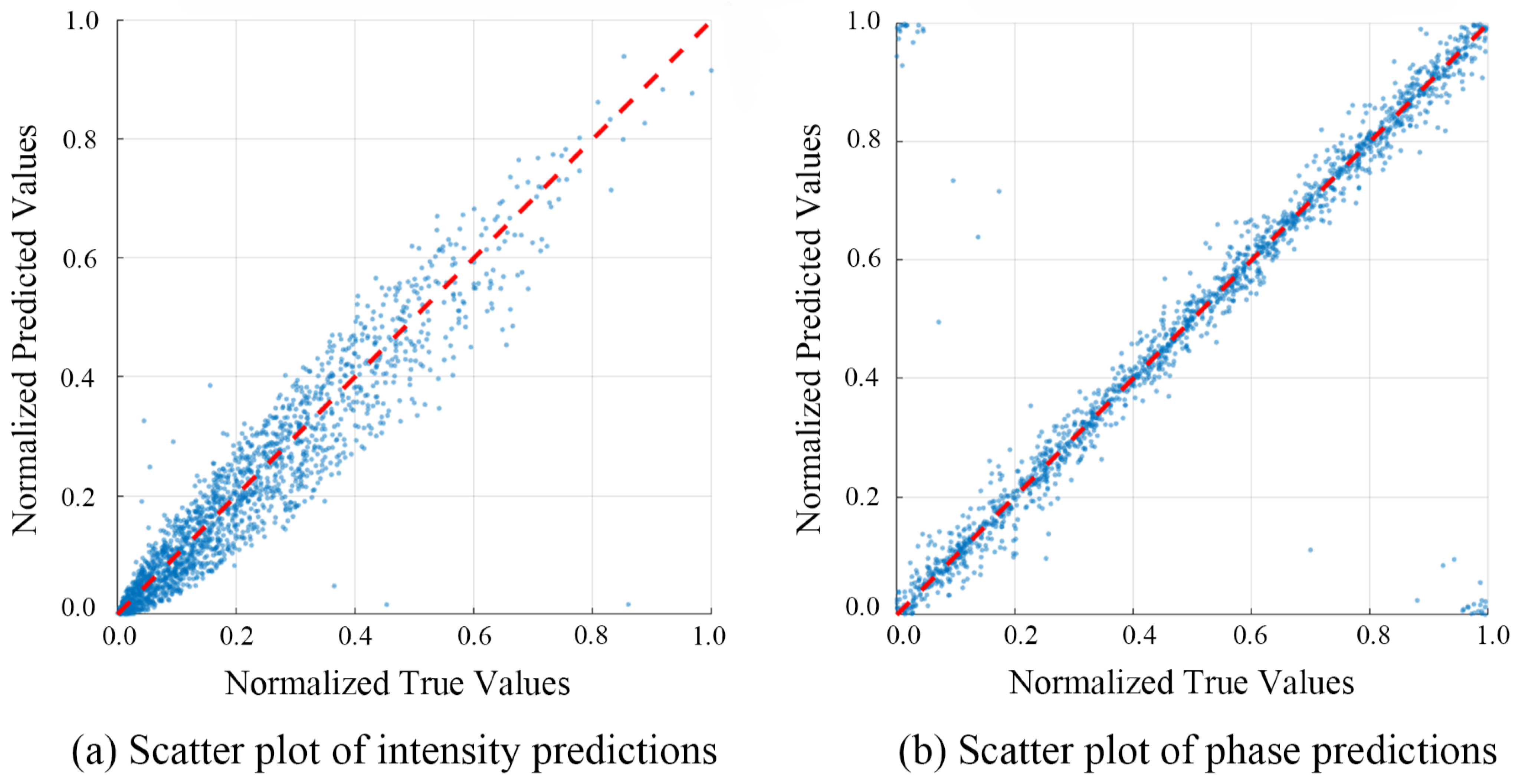
Additionally, this paper uses the original light field dataset from an ideal $1\times 6$ photonic lantern (1500 pairs in total, without 4× data augmentation) to estimate the ideal transmission matrix via least-squares, serving as a control group for Dropout network training. As shown in Equation (4), this process can be expressed as the linear Equation $Y=T\times X$. Here, X is a column vector containing the complex amplitudes of each mode at the input; Y is also a column vector containing the complex amplitudes of each single-mode fiber at the output; and T is a complex matrix, i.e., the transmission matrix we seek, which fully describes the mapping relationship of the light field from the mode space to the spatial ports, including the coupling coefficients between each mode and each fiber as well as the phase delay [26] during transmission. The least-squares method is used to obtain an optimal matrix T that minimizes the sum of squared errors between the predicted output $T\times X$ and the actual observed output Y. Figure 19 shows the prediction results of the ideal matrix for the input light field data; the test light field data aligns with the neural network, totaling 300 pairs.

It should be noted that, since the systematic nonlinear error in the transmission characteristics of photonic lanterns, the linear transmission matrix fails under a large number of random-state distributions, the transmission matrix calculated from a smaller dataset better aligns with the actual transmission characteristics. At the same time, neural networks can fit these nonlinear characteristics. Therefore, as the dataset size increases, the performance of the transmission matrix does not improve; instead, greater deviations occur. To control for variables and facilitate comparison with the neural network model, this paper used only 300 data pairs in calculating the transmission matrix.

As shown in

Table 4. Performance of the Ideal Transmission Matrix Based on the Least Squares Method.

Type	Intensity MSE (Norm. Units)	Intensity R2 (Norm. Units)	Phase MSE (Norm. Units)	Phase R2 (Norm. Units)
Least Squares	$3.175\times {10}^{-3}$	$8.960\times {10}^{-1}$	$1.989\times {10}^{-2}$	$7.574\times {10}^{-1}$
Dropout Network	$9.793\times {10}^{-5}$	$9.973\times {10}^{-1}$	$4.063\times {10}^{-3}$	$9.516\times {10}^{-1}$

and Figure 19, the Dropout network achieves high accuracy in modeling the photonic lantern’s transmission characteristics. The MSE for intensity can reach as low as $9.793\times {10}^{-5}$, and the MSE for phase can reach $4.063\times {10}^{-3}$, which is far superior to the MSE when the transfer matrix predicts the single-mode output. Since the transfer matrix of a photonic lantern is invertible, it follows that if a Dropout network is used to construct a reverse transfer characteristic neural network and trained in reverse using both the single-mode and multimode outputs, the reverse transfer characteristic neural network can also achieve high accuracy.

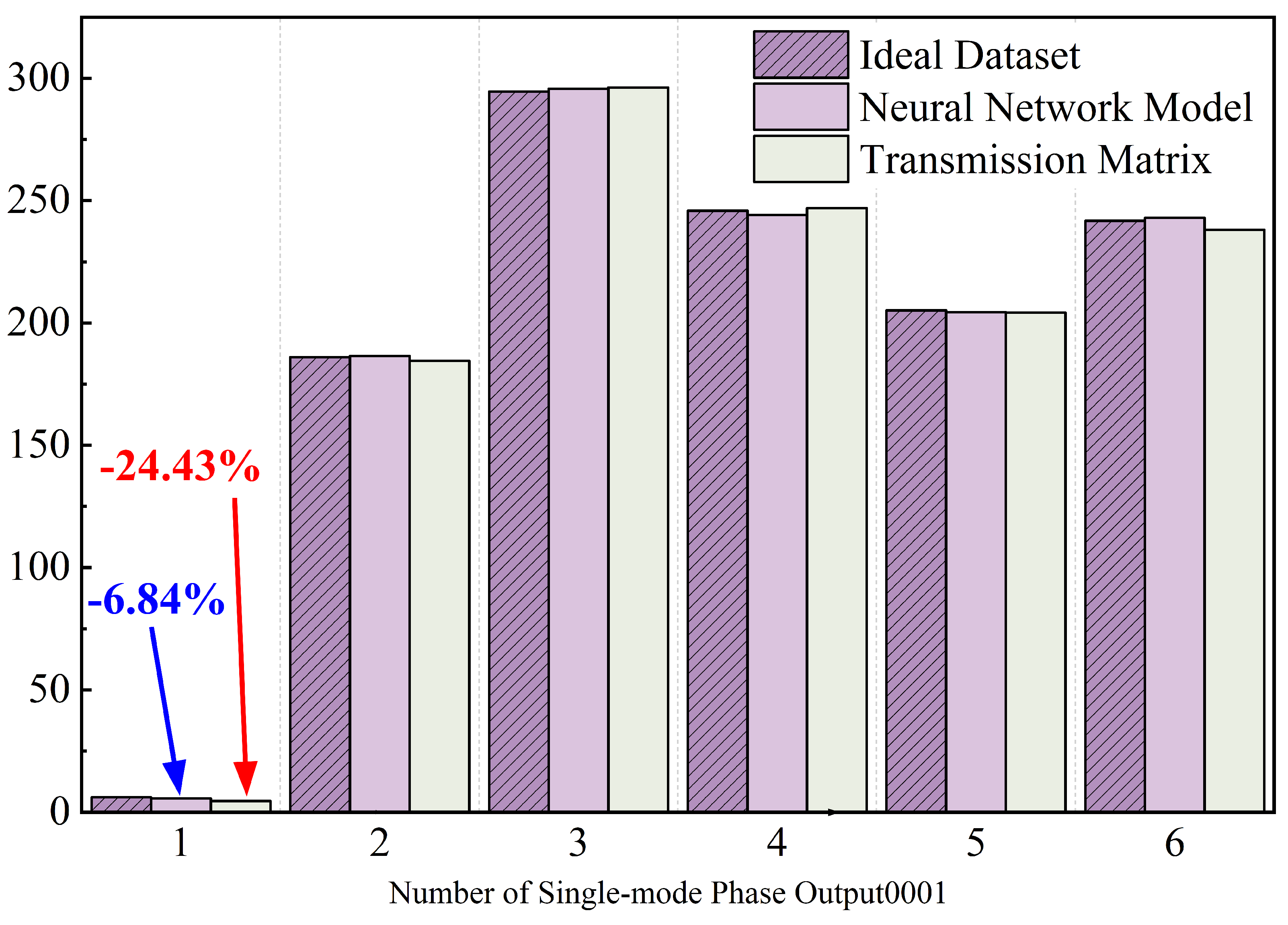
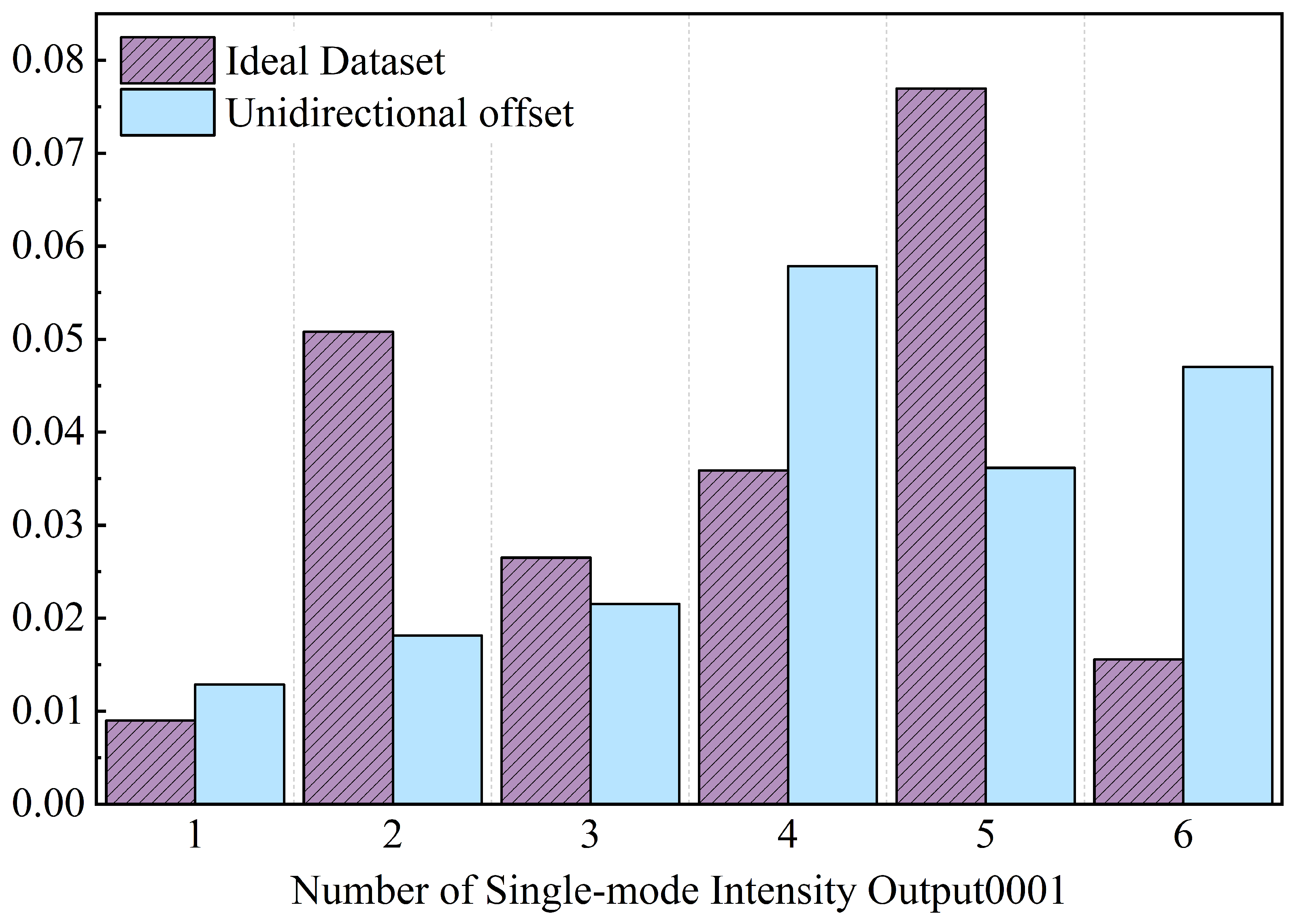
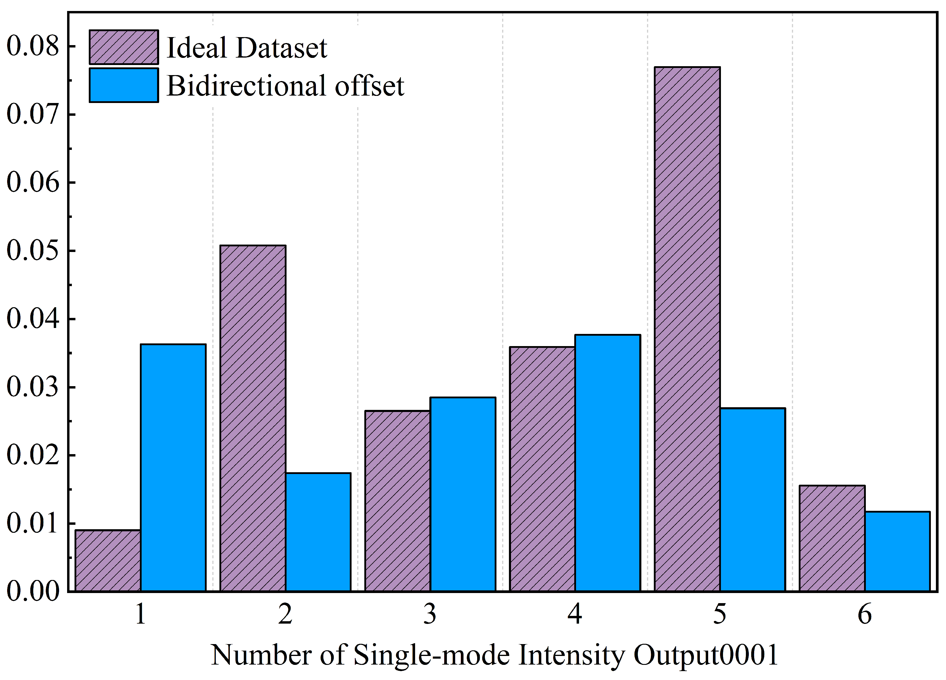
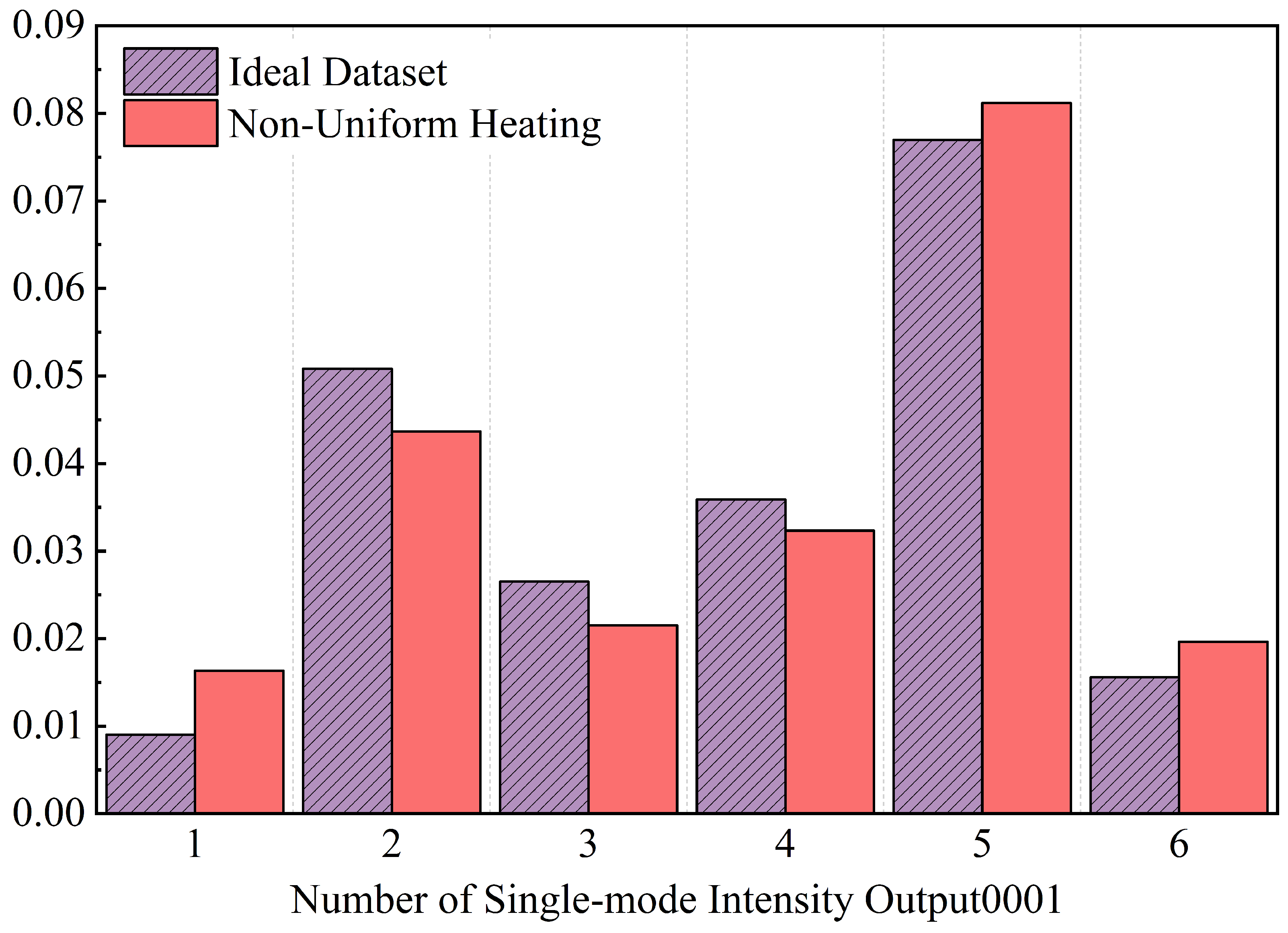
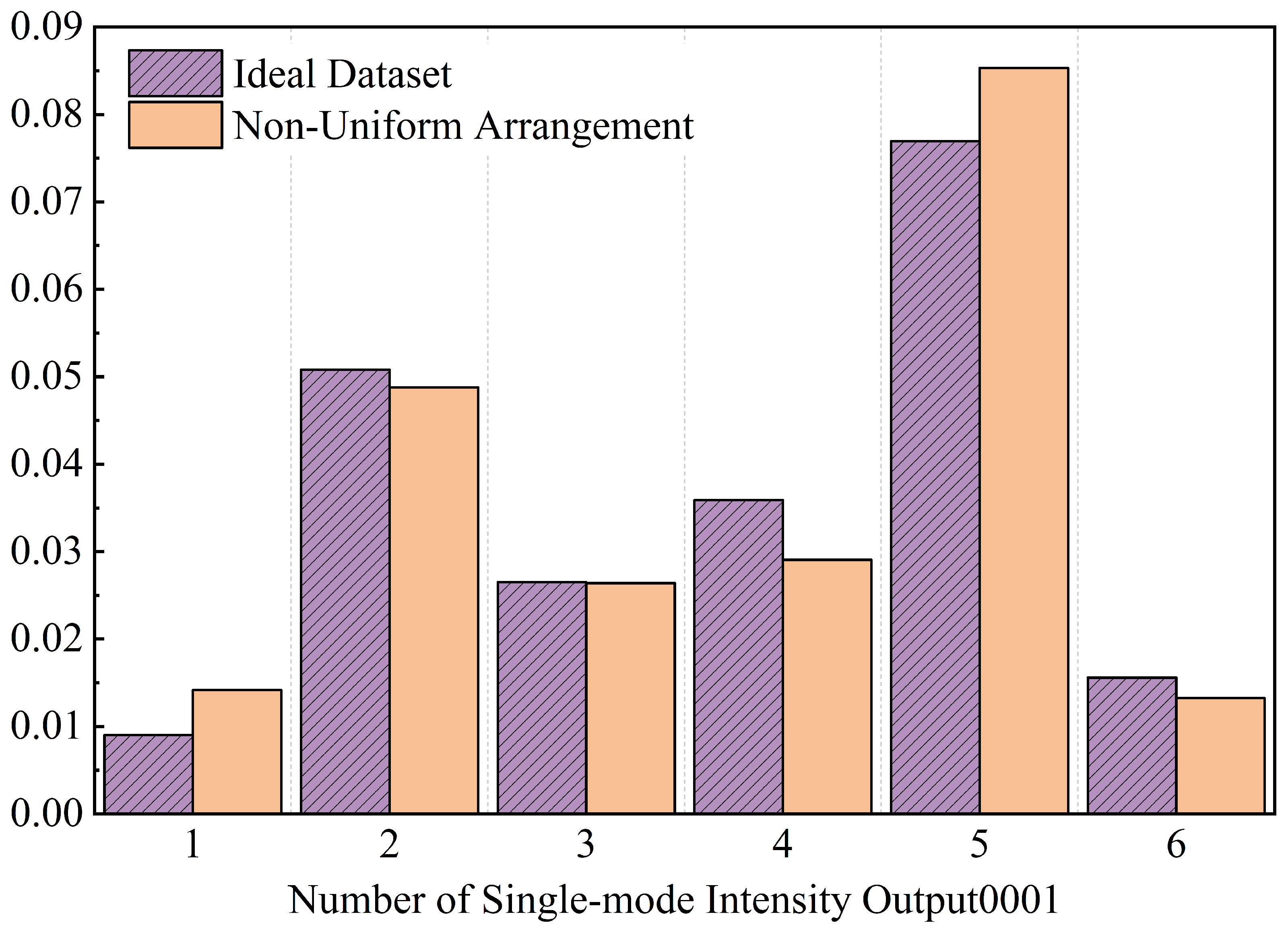
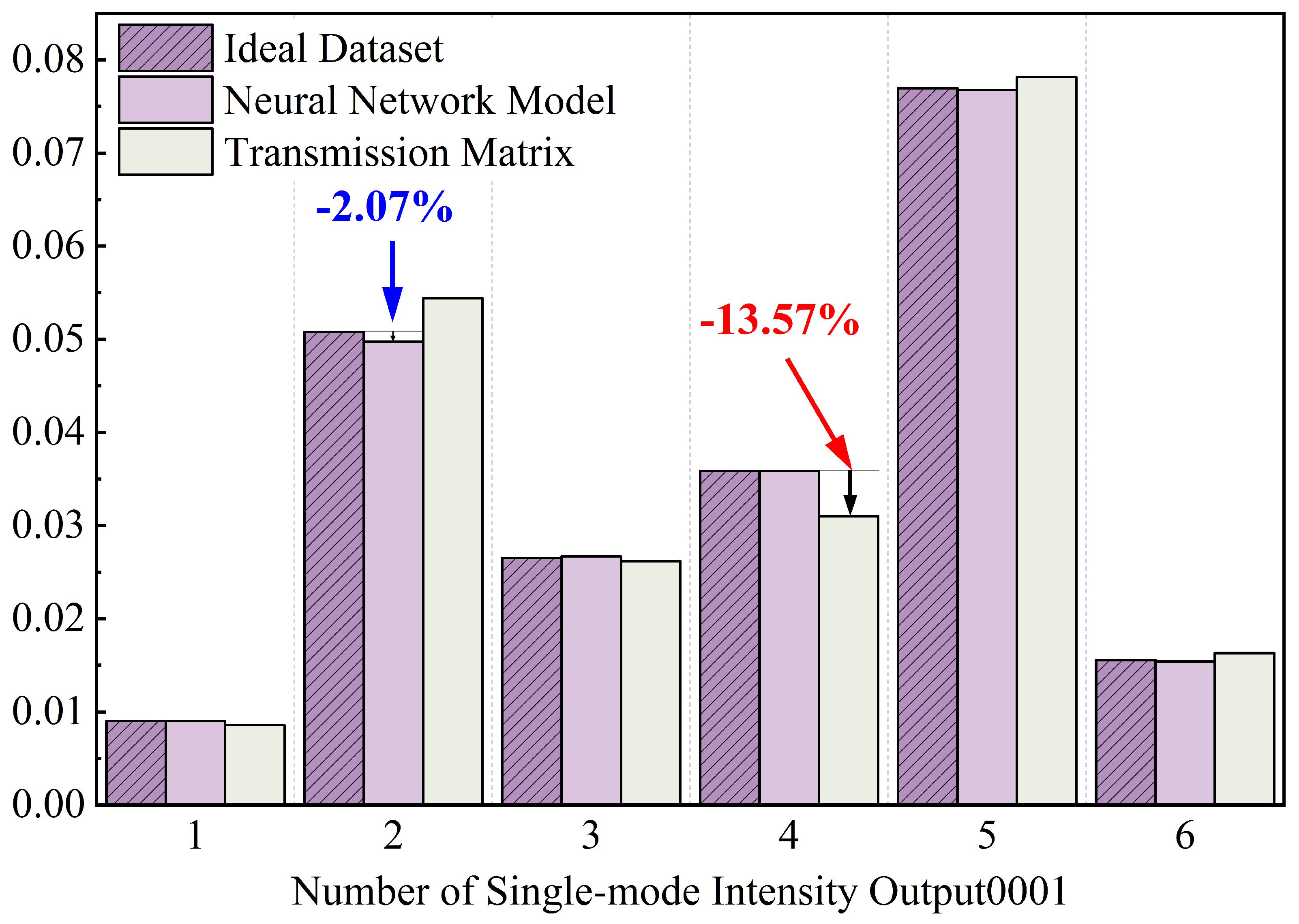
As shown in Figure 20 and Figure 21, as well as

Table 5. Percentage error in optical intensity at the single-mode output of the neural network model and the transfer matrix.

Number of Single-Mode Output0001	Neural Network Model-Intensity	Transmission Matrix-Intensity
1	$0.22\%$	$-4.77\%$
2	$-2.07\%$	$7.09\%$
3	$0.72\%$	$-1.36\%$
4	$-0.03\%$	$-13.57\%$
5	$-0.23\%$	$1.55\%$
6	$-1.09\%$	$4.82\%$

and

Table 6. Percentage phase error of the single-mode output from the neural network model and transfer matrix.

Number of Single-Mode Output0001	Neural Network Model-Phase	Transmission Matrix-Phase
1	$-6.84\%$	$-24.43\%$
2	$0.27\%$	$-0.82\%$
3	$0.38\%$	$0.56\%$
4	$-0.72\%$	$0.43\%$
5	$-0.39\%$	$-0.43\%$
6	$0.50\%$	$-1.51\%$

, taking the intensity and phase of Output 0001 detected by the single-mode port of an ideal $1\times 6$ photonic lantern as an example, for intensity prediction, the maximum error between the neural network model’s predicted intensity and the ideal dataset is within $2.07\%$, whereas the maximum error in intensity prediction by the transfer matrix reaches $13.57\%$. For phase prediction, the maximum error between the neural network model’s predicted phase and the ideal dataset is within $6.84\%$, whereas the maximum error for the transmission matrix’s predicted phase reaches $24.43\%$.

During the experiment, this paper observed a strong positive correlation between dataset size and neural network accuracy: the larger the dataset, the lower the MSE, and the closer the coefficient of determination approaches 1. Currently, a Dropout network is used, with 6000 data points generated via 4-fold data augmentation from 1500 original data points for training. It can be inferred that if the data volume is increased, the accuracy of the transmission characteristic neural network can be improved while ensuring the model does not overfit during training.

When the current model predicts the single-mode output, the MSE for intensity is significantly lower than that for phase. Although the transmission characteristic neural network performs exceptionally well in handling energy distribution, phase information is more complex, and traditional Dropout networks still have certain limitations when processing phase relationships.

Based on our current research, we have considered two optimization schemes for phase feature learning: (1) sine-cosine encoding, which converts phase information from a scalar value to a sine-cosine pair, increasing the input light field dimension from $2N$ to $3N$, thereby preserving periodic information and eliminating boundary discontinuity issues; (2) an optimized complex-valued neural network (CVNN), which demonstrated superior performance to Dropout networks in phase modeling and exhibited greater physical consistency during preliminary experiments, but lagged behind in light intensity prediction accuracy and exhibited significant overfitting that was difficult to resolve, necessitating further optimization.

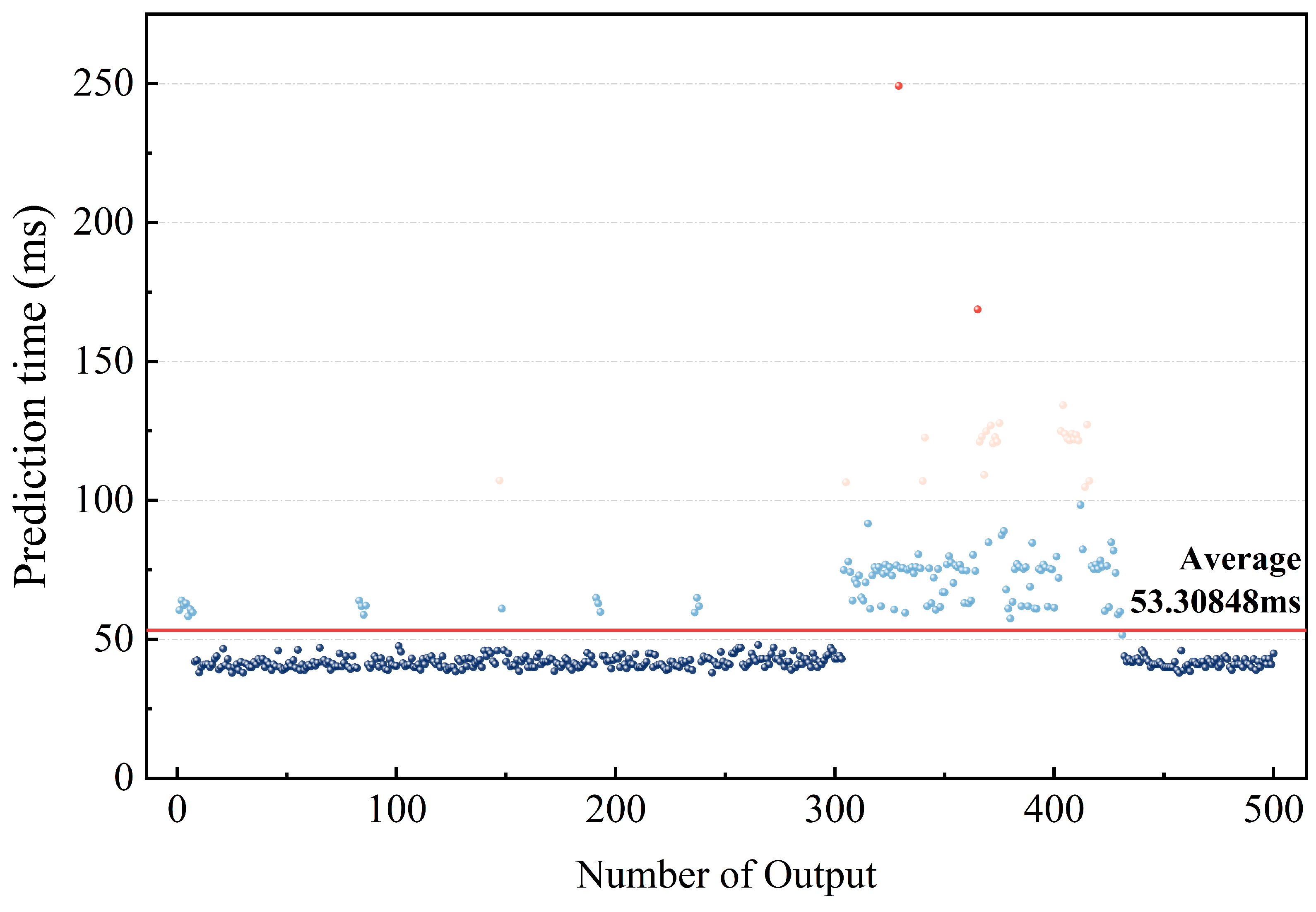
As shown in Figure 22, the transmission characteristic neural network also possesses high-efficiency processing capabilities. Once the photonic lantern transmission characteristic neural network model is trained, it can produce predictions at 53.30848 ms/sample, compared to simulation methods that take 30 to 60 min to obtain single-mode output light-field results, while maintaining high accuracy. The processing time is significantly faster than that of traditional simulation methods, providing a technical pathway for efficient batch processing of light-field data.

4.2. Photonic Lantern Transmission Characteristics Neural Network Model

To verify the neural network model’s calibration capability for the photonic lantern’s transmission characteristics, a systematic cross-validation experiment was designed in this paper. The experiment uses MSE as the core metric for evaluating prediction accuracy, defined as shown in Equation (11):

$$MSE={\displaystyle \frac{1}{N}}{\displaystyle \sum _{i=1}^N}{\left(y_i-{\widehat{y}}_i\right)}^2$$

(11)

where $y_i$ is the true value, ${\widehat{y}}_i$ is the model-predicted value, and N is the number of test samples. A smaller MSE value indicates higher prediction accuracy, while a larger MSE value indicates greater prediction error.

To analyze the accuracy of predictions using MSE, this paper defines the MSE Multiple Index called $m_{\alpha -\beta /\mathrm{ideal}}$, whose value is the ratio of ${\mathrm{MSE}}_{\alpha -\beta }$ to ${\mathrm{MSE}}_{\mathrm{ideal}}$, as shown in Equation (12). ${\mathrm{MSE}}_{\alpha -\beta }$ is defined as the MSE of the $\alpha$ model’s prediction of the $\beta$ dataset, and ${\mathrm{MSE}}_{\mathrm{ideal}}$ is the MSE of the optimal ideal $1\times 6$ photonic lantern neural network model’s prediction of the ideal $1\times 6$ photonic lantern dataset.

$$m_{\alpha -\beta /\mathrm{ideal}}={\displaystyle \frac{{\mathrm{MSE}}_{\alpha -\beta }}{{\mathrm{MSE}}_{\mathrm{ideal}}}}$$

(12)

In this paper, only the neural network model for the optimal ideal $1\times 6$ photonic lantern, trained on a large dataset (6000 pairs of extended data and 1500 pairs of original data), is used to predict different datasets. The neural network model for the manufacturing error photonic lantern, trained on a small dataset (500 pairs of original data), is used solely to predict the corresponding manufacturing error dataset.

Table 7. Intensity Norm.MSE Matrix.

Neural Networks Model	Photonic Lantern Dataset
	Ideal	Unidirectional Offset	Bidirectional Offset	Non-Uniform Heating	Non-Uniform Arrangement
Ideal	$2.418\times {10}^{-3}$	$3.272\times {10}^{-2}$	$5.149\times {10}^{-2}$	$9.849\times {10}^{-3}$	$6.339\times {10}^{-3}$
Unidirectional offset		$9.660\times {10}^{-3}$
Bidirectional offset			$4.362\times {10}^{-3}$
Non-Uniform Heating				$9.415\times {10}^{-3}$
Non-Uniform Arrangement					$5.282\times {10}^{-3}$

and

Table 8. Intensity MSE Multiple Index $m_{\alpha -\beta /\mathrm{ideal}}$ Matrix.

Neural Networks Model	Photonic Lantern Dataset
	Ideal	Unidirectional Offset	Bidirectional Offset	Non-Uniform Heating	Non-Uniform Arrangement
Ideal	1	13.533	21.298	4.074	2.622
Unidirectional offset		3.995
Bidirectional offset			1.804
Non-Uniform Heating				3.894
Non-Uniform Arrangement					2.185

present the normalized MSE and the MSE Multiple Index $m_{\alpha -\beta /\mathrm{ideal}}$ for luminance across various models and test sets.

Analysis of the above data shows that the neural network model for the photonic lantern’s transmission characteristics can effectively detect manufacturing errors.

Analysis of the first row of data in Table 8 reveals that, when using the ideal model to predict the manufacturing error dataset, the MSE for light intensity increased significantly, from 2.622 to 21.298. These data indicate a significant difference in the transmission characteristics between photonic lanterns with manufacturing errors and ideal photonic lanterns. Therefore, neural network models trained on ideal photonic lantern datasets and transmission matrices are not suitable for calculating the transmission characteristics of photonic lanterns with manufacturing errors. Furthermore, as concluded in Section 4.1, the MSE of the ideal photonic lantern neural network model is far superior to that of the transfer matrix when predicting the single-mode output. These data prove that the neural network model outperforms the transfer matrix in calibrating photonic lanterns with manufacturing errors. If the transfer matrix is used to predict the single-mode output of a photonic lantern with manufacturing errors, the error will be significantly greater than that of the neural network model.

By training a photonic lantern neural network model, we performed predictions on a test set of 500 pairs of similar photonic lanterns and obtained the model’s MSE for light intensity along the diagonal. We found that the MSE was amplified by a factor of 1.804 to 3.995. Given that the neural network model for manufacturing error photonic lanterns was trained on only 500 pairs of original data, the model’s prediction accuracy (MSE) is expected to be somewhat lower than that of the ideal photonic lantern model trained on a dataset of 6000 pairs (1500 pairs of original data). This further corroborates the inference in Section 4.1: there is a strong positive correlation between dataset size and neural network accuracy—the larger the dataset, the lower the MSE.

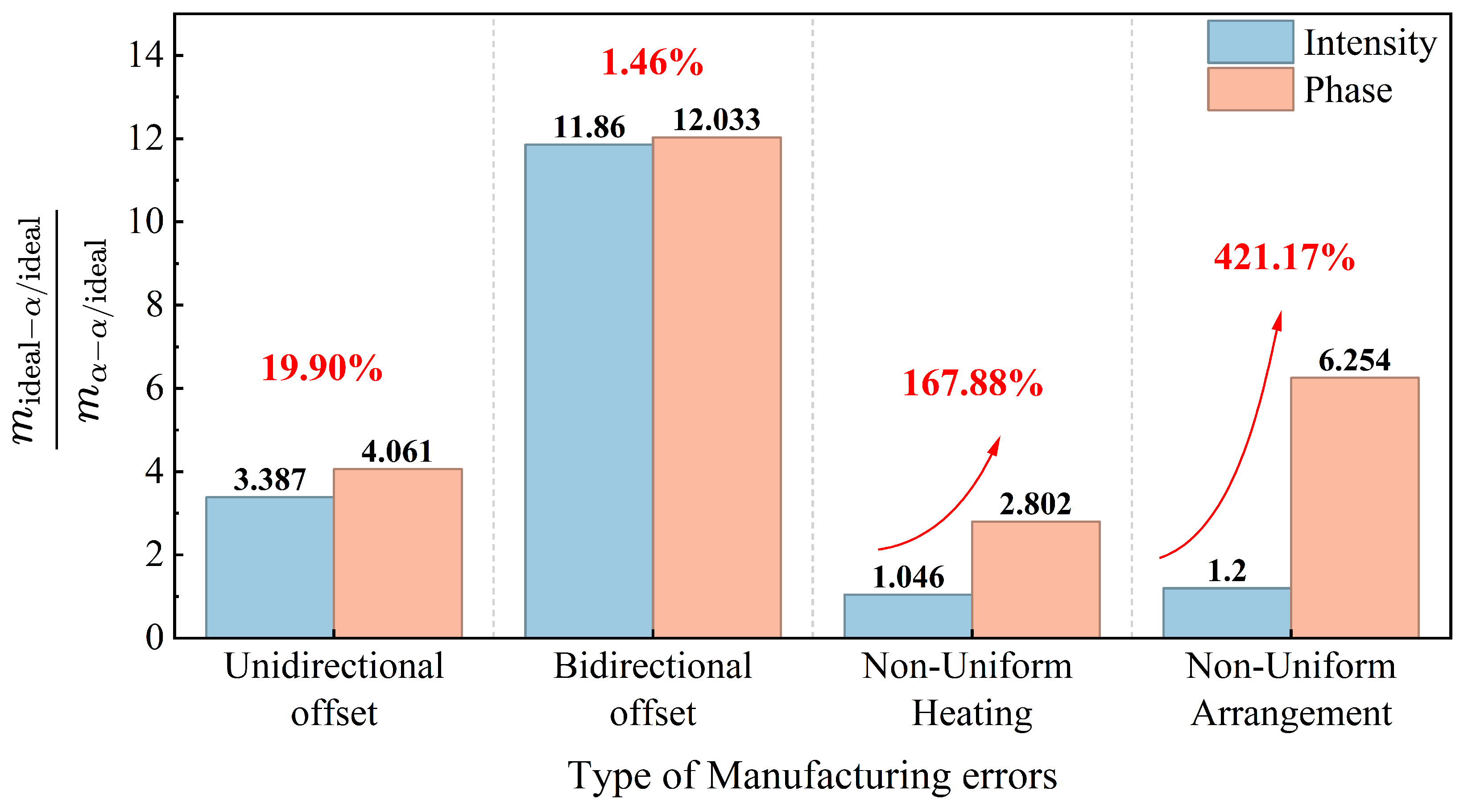
As shown in

Table 9. Multiple Index m for Intensity MSE of Photonic Lanterns with Manufacturing Errors.

Type of Manufacturing Errors (Model/Dataset α)	${\mathit{m}}_{\mathit{\alpha }-\mathit{\alpha }/\mathbf{ideal}}$	${\mathit{m}}_{\mathbf{ideal}-\mathit{\alpha }/\mathbf{ideal}}$	${\displaystyle \frac{{\mathit{m}}_{\mathbf{ideal}-\mathit{\alpha }/\mathbf{ideal}}}{{\mathit{m}}_{\mathit{\alpha }-\mathit{\alpha }/\mathbf{ideal}}}}$
Unidirectional
offset	3.995	13.533	3.387
Bidirectional
offset	1.804	21.298	11.860
Non-Uniform
Heating	3.894	4.074	1.046
Non-Uniform
Arrangement	2.185	2.622	1.200

, compared to the light intensity prediction accuracy of the ideal photonic lantern neural network model on the manufacturing error training set, the accuracy of the Unidirectional Offset neural network model increased by 3.387 times, the Bidirectional Offset neural network model increased by 11.860 times, and the Non-Uniform Heating neural network model increased by 1.046 times. Furthermore, the Non-Uniform Arrangement neural network model saw a 1.200-fold improvement in accuracy. Analysis indicates that, compared to manufacturing errors caused by non-uniform heat input and non-uniform arrangement, the neural network faces relatively greater difficulty in capturing the transmission characteristics of the latter two types of manufacturing errors during small-sample tuning, as shown below. Given that the MSE deviations for non-uniform heat input and non-uniform arrangement are relatively small in the ideal model, it can be inferred that the impact of taper non-uniformness-related errors on the transmission characteristics of the photonic lantern is relatively smaller compared to that of misalignment welding.

Similarly,

Table 10. Phase Norm.MSE Matrix.

Neural Networks Model	Photonic Lantern Dataset
	Ideal	Unidirectional Offset	Bidirectional Offset	Non-Uniform Heating	Non-Uniform Arrangement
Ideal	$3.160\times {10}^{-3}$	$7.873\times {10}^{-2}$	$5.149\times {10}^{-2}$	$7.218\times {10}^{-2}$	$6.773\times {10}^{-2}$
Unidirectional offset		$1.939\times {10}^{-2}$
Bidirectional offset			$9.498\times {10}^{-3}$
Non-Uniform Heating				$2.576\times {10}^{-2}$
Non-Uniform Arrangement					$1.083\times {10}^{-2}$

and

Table 11. Phase MSE Multiple Index $m_{\alpha -\beta /\mathrm{ideal}}$ Matrix.

Neural Networks Model	Photonic Lantern Dataset
	Ideal	Unidirectional Offset	Bidirectional Offset	Non-Uniform Heating	Non-Uniform Arrangement
Ideal	1	24.914	36.172	22.84	21.432
Unidirectional offset		6.135
Bidirectional offset			3.006
Non-Uniform Heating				8.151
Non-Uniform Arrangement					3.427

summarize the normalized MSE and the MSE Multiple Index for luminous intensity across different test sets for each model.

Analysis of the first row of data in Table 11 reveals that when using the ideal model to predict the manufacturing error dataset, the phase MSE increased significantly, from 21.432 to 36.172 times, a more pronounced increase than the variation in light intensity. These data indicate that changes in transmission characteristics caused by manufacturing errors have a particularly significant impact on phase, further corroborating the presence of significant differences between the transmission characteristics of photonic lanterns with manufacturing errors and those of ideal photonic lanterns.

Analysis of the phase MSE for the photonic lantern model with manufacturing errors along the diagonal shows that the MSE increased by a factor of 3.006 to 8.151. It can be inferred that, under small-sample conditions, the neural network model can still be further optimized to improve phase prediction accuracy. This also supports the conclusion in Section 4.1: traditional Dropout networks still have certain limitations when handling phase relationships.

As shown in

Table 12. Multiple Index m for Phase MSE of Photonic Lanterns with Manufacturing Errors.

Type of Manufacturing Errors (Model/Dataset α)	${\mathit{m}}_{\mathit{\alpha }-\mathit{\alpha }/\mathbf{ideal}}$	${\mathit{m}}_{\mathbf{ideal}-\mathit{\alpha }/\mathbf{ideal}}$	${\displaystyle \frac{{\mathit{m}}_{\mathbf{ideal}-\mathit{\alpha }/\mathbf{ideal}}}{{\mathit{m}}_{\mathit{\alpha }-\mathit{\alpha }/\mathbf{ideal}}}}$
Unidirectional
offset	6.135	24.914	4.061
Bidirectional
offset	3.006	36.172	12.033
Non-Uniform
Heating	8.151	22.84	2.802
Non-Uniform
Arrangement	3.427	21.432	6.254

, compared to the phase prediction accuracy of the ideal photonic lantern neural network model on the manufacturing error training set, the accuracy of the Unidirectional Offset neural network model improved by a factor of 4.061, the Bidirectional Offset neural network model by a factor of 12.033, and the Non-Uniform Heating neural network model by a factor of 2.802, and the Non-Uniform Arrangement neural network model achieved a 6.254-fold improvement.

As shown in Figure 23, since the phase transmission characteristics of photonic lanterns with manufacturing errors vary significantly compared to those of ideal photonic lanterns, and the variation in phase transmission characteristics is greater than that in light intensity transmission characteristics, the neural network models demonstrate improved accuracy when handling all four types of manufacturing errors compared to light intensity. This is particularly evident for non-uniform arrangement, where accuracy improved from 1.200 times that of light intensity to 6.254 times; and for non-uniform intensity distribution, accuracy improved from 1.046 times that of the intensity to 2.802 times.

5. Conclusions

This paper employs a neural network to characterize photonic lantern devices by training a model of their transmission characteristics. It achieved a predicted intensity MSE of $9.793\times {10}^{-5}$ for an ideal $1\times 6$ photonic lantern from the multimode end to the single-mode end, representing a 32.42-fold improvement over the intensity predictions MSE using the transmission matrix. The predicted phase MSE reached $3.814\times {10}^{-3}$, representing a 4.90-fold improvement over the MSE of phase predictions based on the transmission matrix. This study also found that the transmission characteristics of photonic lanterns with manufacturing errors differ significantly from those of ideal photonic lanterns; the neural network model for photonic lantern transmission characteristics achieves higher accuracy in modeling photonic lanterns with manufacturing errors than traditional modeling methods. When using the ideal model to predict the manufacturing error dataset, the intensity MSE increased by up to 21.298 times, and the phase MSE increased by up to 36.172 times, enabling the reliable detection of photonic lanterns with manufacturing errors. Compared to traditional simulation methods, the neural network model for photonic lantern transmission characteristics can compute light-field outputs more efficiently after training; the time required to process a single light field is reduced from minutes with traditional methods to milliseconds in this study. Additionally, this study found that the number of samples is significantly correlated with model accuracy. If the dataset is appropriately expanded, it is anticipated that accuracy will further improve, and the neural network model still holds considerable potential for calibrating the nonlinear relationships of photonic lanterns. However, using MSE as the sole evaluation metric can only determine the presence of manufacturing errors but cannot distinguish their specific types.

In future work, we will proceed to fabricate photonic lanterns and conduct further research on the transmission characteristic models—particularly those with manufacturing errors—by combining simulation models with experimental data. We will prepare a series of photonic lantern samples with known, controllable manufacturing errors (such as core offset and diameter deviation) and measure their transmission characteristics. By systematically comparing the predictions from our model (trained on simulation data) with actual measurement data, we will quantitatively evaluate the model’s generalization capability and prediction accuracy under real-world conditions. Additionally, we will design and fabricate various $1\times N$ photonic lantern models to further investigate how this neural network model can be applied to photonic lanterns with a wider range of configurations. In the next phase of research, we plan to introduce additional evaluation metrics and combine them with explainable artificial intelligence techniques to achieve not only detection but also classification of manufacturing error types.

References

1. Birks, T.A.; Gris-Sánchez, I.; Yerolatsitis, S.; Leon-Saval, S.G.; Thomson, R.R. The photonic lantern. Adv. Opt. Photonics 2015, 7, 107–167. [Google Scholar] [CrossRef]
2. Fontaine, N.K.; Ryf, R.; Bland-Hawthorn, J.; Leon-Saval, S.G. Geometric requirements for photonic lanterns in space division multiplexing. Opt. Express 2012, 20, 27123–27132. [Google Scholar] [CrossRef]
3. He, Y.; Chen, X. Optical Characteristic Research on Fiber Bragg Gratings Utilizing Finite Element and Eigenmode Expansion Methods. Sensors 2014, 14, 10876–10894. [Google Scholar] [CrossRef] [PubMed]
4. Diab, M.; Minardi, S. Modal analysis using photonic lanterns coupled to arrays of waveguides. Opt. Lett. 2019, 44, 1718–1721. [Google Scholar] [CrossRef] [PubMed]
5. Sweeney, D.; Norris, B.R.; Tuthill, P.; Scalzo, R.; Wei, J.; Betters, C.H.; Leon-Saval, S.G. Learning the lantern: Neural network applications to broadband photonic lantern modeling. J. Astron. Telesc. Instrum. Syst. 2021, 7, 028007. [Google Scholar] [CrossRef]
6. Wu, W.; Huang, Q.; Wang, C.; Huang, Y.; Li, Y.; Chen, L.; Zhao, J.; Ertman, S.; Halendy, M.; Xu, O.; et al. All-optical-fiber photonic lantern operates from O-band to 2 µm wavelength band and beyond. Opt. Laser Technol. 2025, 192, 113850. [Google Scholar] [CrossRef]
7. Taras, A.K.; Norris, B.R.; Betters, C.; Ross-Adams, A.; Tuthill, P.G.; Wei, J.; Leon-Saval, S. Illuminating the lantern: Coherent, spectro-polarimetric characterization of a multimode converter. Opt. Express 2026, 34, 1012–1025. [Google Scholar] [CrossRef] [PubMed]
8. Boyd, G.D.; Gordon, J.P. Confocal multimode resonator for millimeter through optical wavelength masers. Bell Syst. Tech. J. 1961, 40, 489–508. [Google Scholar] [CrossRef]
9. Kogelnik, H.; Li, T. Laser beams and resonators. Appl. Opt. 1966, 5, 1550–1567. [Google Scholar] [CrossRef]
10. Arnaud, J.A.; Kogelnik, H. Gaussian light beams with general astigmatism. Appl. Opt. 1969, 8, 1687–1693. [Google Scholar] [CrossRef]
11. Ganiel, U.; Hardy, A. Eigenmodes of optical resonators with mirrors having Gaussian reflectivity profiles. Appl. Opt. 1976, 15, 2145–2149. [Google Scholar] [CrossRef]
12. Casperson, L.W. Beam modes in complex lenslike media and resonators. J. Opt. Soc. Am. 1976, 66, 1373–1379. [Google Scholar] [CrossRef]
13. Gloge, D. Weakly guiding fibers. Appl. Opt. 1971, 10, 2252–2258. [Google Scholar] [CrossRef]
14. Paiano, G.; Pellicoro, M. Propagation constant of weakly guiding optical fibers: A new eigenvalue condition. J. Light. Technol. 2001, 19, 1592. [Google Scholar] [CrossRef]
15. Kogelnik, H.; Ramaswamy, V. Scaling rules for thin-film optical waveguides. Appl. Opt. 1974, 13, 1857–1862. [Google Scholar] [CrossRef] [PubMed]
16. Collins, S.A., Jr. Lens-system diffraction integral written in terms of matrix optics. J. Opt. Soc. Am. 1970, 60, 1168–1177. [Google Scholar] [CrossRef]
17. Streda, P.; Kucera, J.; MacDonald, A. Edge states, transmission matrices, and the Hall resistance. Phys. Rev. Lett. 1987, 59, 1973. [Google Scholar] [CrossRef]
18. Hornik, K.; Stinchcombe, M.; White, H. Multilayer feedforward networks are universal approximators. Neural Netw. 1989, 2, 359–366. [Google Scholar] [CrossRef]
19. LeCun, Y.; Bengio, Y.; Hinton, G. Deep learning. Nature 2015, 521, 436–444. [Google Scholar] [CrossRef]
20. Mathew, N.M.; Grüner-Nielsen, L.; Castaneda, M.A.U.; Rottwitt, K. A Novel Fabrication Method for Photonic Lanterns. In Proceedings of the 2018 Optical Fiber Communications Conference and Exposition (OFC); IEEE: Piscataway, NJ, USA, 2018. [Google Scholar] [CrossRef]
21. Leon-Saval, S.G.; Argyros, A.; Bland-Hawthorn, J. Photonic lanterns: A study of light propagation in multimode to single-mode converters. Opt. Express 2010, 18, 8430–8439. [Google Scholar] [CrossRef]
22. Brambilla, G.; Finazzi, V.; Richardson, D.J. Ultra-low-loss optical fiber nanotapers. Opt. Express 2004, 12, 2258–2263. [Google Scholar] [CrossRef]
23. Gross, S.; Withford, M.J. Ultrafast-laser-inscribed 3D integrated photonics: Challenges and emerging applications. Nanophotonics 2015, 4, 332–352. [Google Scholar] [CrossRef]
24. Srivastava, N.; Hinton, G.; Krizhevsky, A.; Sutskever, I.; Salakhutdinov, R. Dropout: A simple way to prevent neural networks from overfitting. J. Mach. Learn. Res. 2014, 15, 1929–1958. [Google Scholar]
25. Han, X.; Papyan, V.; Donoho, D.L. Neural collapse under mse loss: Proximity to and dynamics on the central path. arXiv 2021, arXiv:2106.02073. [Google Scholar]
26. Montoya, J.; Aleshire, C.; Hwang, C.; Fontaine, N.K.; Velázquez-Benítez, A.; Martz, D.H.; Fan, T.Y.; Ripin, D. Photonic lantern adaptive spatial mode control in LMA fiber amplifiers. Opt. Express 2016, 24, 3405–3413. [Google Scholar] [CrossRef]
Figure 1. Structure of the photonic lantern.
Photonics 13 00496 g001
Figure 2. Schematic of near-field intensity and phase distributions for typical LP modes.
Photonics 13 00496 g002
Figure 3. Cross-sectional view of the 1 × 6 photonic lantern.
Photonics 13 00496 g003
Figure 4. Intensity and phase images of the input light field at the multimode end and the output at the single-mode end of an ideal 1 × 6 photonic lantern.
Photonics 13 00496 g004
Figure 5. Structure of ideal photonic lantern.
Photonics 13 00496 g005
Figure 6. Structure of lateral-offset splicing.
Photonics 13 00496 g006
Figure 7. Intensity and phase images of the single-mode output from a 1 × 6 photonic lantern with offset splicing; (a,b) show the Unidirectional offset model, while (c,d) show the Bidirectional offset model.
Photonics 13 00496 g007
Figure 8. Intensity of the output from the single-mode end of a 1 × 6 photonic lantern with offset splicing (Unidirectional offset model).
Photonics 13 00496 g008
Figure 9. Intensity of the output from the single-mode end of a 1 × 6 photonic lantern with offset splicing (Bidirectional offset model).
Photonics 13 00496 g009
Figure 10. Non-uniform heating (when the end coordinates and dimensions of the core segments are multiplied by a factor of 0.7).
Photonics 13 00496 g010
Figure 11. Intensity and phase images of the single-mode output from a 1 × 6 photonic lantern with non-uniform heating.
Photonics 13 00496 g011
Figure 12. Intensity of the output from the single-mode end of a 1 × 6 photonic lantern with non-uniform heating.
Photonics 13 00496 g012
Figure 13. Non-uniform arrangement.
Photonics 13 00496 g013
Figure 14. Intensity and phase images of the single-mode output from a 1 × 6 photonic lantern with non-uniform arrangement.
Photonics 13 00496 g014
Figure 15. Intensity of the output from the single-mode end of a 1 × 6 photonic lantern with non-uniform arrangement.
Photonics 13 00496 g015
Figure 16. Overview of a Dropout network when p = 0 .
Photonics 13 00496 g016
Figure 17. Dropout network when p > 0 , using p = 0.2 as an example.
Photonics 13 00496 g017
Figure 18. Training Process and Results of the Dropout Network.
Photonics 13 00496 g018
Figure 19. Scatter plot of transmission matrix prediction results.
Photonics 13 00496 g019
Figure 20. Intensity comparison at the single-mode output of the ideal dataset, the neural network model, and the transmission matrix.
Photonics 13 00496 g020
Figure 21. Phase comparison at the single-mode output of the ideal dataset, the neural network model, and the transmission matrix.
Photonics 13 00496 g021
Figure 22. Prediction time of the Trained Neural Network.
Photonics 13 00496 g022
Figure 23. m ideal α / ideal / m α α / ideal of intensity versus phase.
Photonics 13 00496 g023