Mie-Scattering-Based Simulation of Underwater Multispectral LiDAR Propagation and Optimal Wavelength Selection

Abstract

Multispectral LiDAR can simultaneously obtain distance and spectral information and shows great potential for underwater detection. However, absorption and scattering caused by suspended particles in water lead to energy attenuation and multiple scattering, which affect echo intensity and ranging accuracy, while the propagation characteristics under multi-wavelength conditions remain insufficiently studied. In this study, a simplified underwater propagation simulation model for multispectral LiDAR is established based on the equivalent spherical-particle assumption, combining Mie scattering theory with a semi-analytical Monte Carlo method. The effects of particle size on echo intensity and ranging error are analyzed under fixed concentration conditions. Based on this model, a detection-threshold-constrained optimal wavelength selection criterion is formulated. Multi-distance analysis (3, 5, 8, and 15 m) confirms that the preferred wavelength is primarily governed by particle size and remains stable across depths. The results show that the optimal detection wavelength shifts with particle size, being about 560 nm for fine particles and gradually moving toward the 400–480 nm blue–green band for larger particles. Experimental validation shows that the simulation-based ranging correction reduces RMSE by 9.4–25.9% (average 18.1%) and MAE by 11.8–29.7% (average 22.0%) across five experimental distances. The results provide a preliminary reference for wavelength selection in multispectral LiDAR systems under simplified conditions.

1. Introduction

The ocean plays an essential role in global climate regulation, biogeochemical cycles, and marine resource exploitation. High-precision observation of the marine environment is therefore fundamental to oceanographic research [1]. With the rapid development of underwater sensor networks and autonomous underwater vehicles, marine surveys have gained increasing scientific, economic, and strategic importance [2]. Multispectral LiDAR has great potential for simultaneously acquiring spatial and spectral information, particularly in challenging underwater environments [3]. By providing high-precision spatial measurements together with detailed spectral characteristics, multispectral LiDAR enables more accurate observation and characterization of underwater objects. These capabilities significantly expand the application scope of LiDAR technology in complex underwater environments. Consequently, developing effective optical propagation simulation methods for multispectral LiDAR in underwater detection has become increasingly important.

In recent years, with the rapid development of laser and spectral detection technology, multispectral and hyperspectral LiDAR have gradually become important directions in laser remote sensing. Early studies mainly focused on terrestrial vegetation monitoring, where multi-wavelength laser systems were used to obtain spectral information in visible and near-infrared bands for retrieving vegetation indices such as the normalized difference vegetation index (NDVI) and photochemical reflectance index (PRI) [4,5]. With the development of technology, hyperspectral LiDAR systems have emerged. The Finnish Geospatial Research Institute developed a multi-channel hyperspectral LiDAR system capable of acquiring spectral information from the visible to near-infrared range, which has been successfully applied to forest reflectance measurements and vegetation parameter retrieval [6,7]. Subsequently, several research institutions, including Wuhan University and the Aerospace Information Research Institute of the Chinese Academy of Sciences, have developed hyperspectral LiDAR systems with dozens of spectral channels, enabling higher spectral resolution in remote sensing observations [8,9,10,11].As the number of spectral channels and spectral resolution of multispectral LiDAR systems continue to increase, their application scope has gradually expanded from terrestrial remote sensing to underwater exploration in complex aquatic environments. In recent years, multispectral LiDAR has been applied in underwater archaeology [12], seabed habitat mapping [13], underwater material identification [14] and underwater sediments classification [15]. Zhang et al. developed a hyperspectral LiDAR system for underwater exploration, achieving multispectral detection in the 450–700 nm wavelength range and generating hyperspectral point cloud data [16]. Ma et al. constructed a multispectral LiDAR system based on an acousto-optic tunable filter (AOTF) operating in the 560–800 nm range, and successfully performed underwater spherical target classification using a support vector machine (SVM) algorithm [17]. These studies demonstrate the great potential of multispectral LiDAR for underwater detection in complex environments.

Water is a highly complex optical medium whose composition and density vary continuously in time and space, making laser propagation in water highly stochastic. Consequently, understanding the propagation characteristics of underwater lasers has become an important research topic. Seawater contains large amounts of suspended substances, such as suspended sediments and phytoplankton, which can absorb and scatter incident laser radiation, leading to rapid attenuation of laser energy during propagation. Among these processes, Mie scattering caused by suspended particles is one of the primary sources of optical attenuation in seawater and has a significant influence on laser propagation depth and echo intensity [18]. Mie scattering theory can accurately describe the interaction between electromagnetic waves and spherical particles and is therefore widely used to calculate optical parameters of waterborne particles, including the scattering coefficient, attenuation coefficient, and scattering phase function [19]. Previous studies have applied Mie scattering theory to investigate the effects of particle size and concentration on laser propagation in water. The results indicate that variations in particle size and concentration can significantly alter the scattering properties of seawater, thereby affecting laser propagation distance and received intensity [17,18]. Therefore, establishing a particle optical model based on Mie scattering theory is essential for describing the optical properties of seawater in studies of underwater laser propagation.

The main approaches for analyzing light scattering in water include analytical methods, experimental methods, and Monte Carlo (MC) simulations [20]. Analytical approaches usually rely on idealized assumptions and are therefore difficult to apply to complex water environments. Some studies have applied the lidar equation for analysis, but its applicability remains limited [21]. Experimental methods can provide direct observations but are often constrained by experimental conditions. In comparison, combining experimental studies with MC simulations provides greater flexibility while maintaining physical realism and has been proven to be an effective approach [22].

The Monte Carlo (MC) method has been widely applied to studies of underwater light propagation and oceanic LiDAR signal modeling. For example, a polarized Monte Carlo model for shipborne oceanic LiDAR has been developed and validated using experimental measurements [23]. In addition, MC methods have also been employed in studies of underwater laser imaging and detection systems, where numerical simulations are used to analyze imaging performance under different environmental conditions [22]. However, MC simulations usually require a large number of photons to obtain statistically stable results, which leads to relatively low computational efficiency. To address this limitation, the semi-analytical Monte Carlo method has been proposed to improve computational efficiency [24]. By statistically estimating the probability that photons return directly to the receiver after each scattering event, the number of simulated photons can be significantly reduced while maintaining accuracy. For instance, Huang et al. combined ray-tracing with a semi-analytical Monte Carlo model to simulate underwater target echoes for a UAV-based oceanic LiDAR system [25]. Similarly, Wang et al. used a semi-analytical Monte Carlo method to evaluate multispectral underwater LiDAR signals under different chlorophyll conditions [26]. In underwater laser propagation simulations, the optical properties of suspended particles play a critical role in determining propagation characteristics. The absorption and scattering properties of water significantly affect the propagation of LiDAR echo signals [27]. Previous studies have combined Mie scattering theory with the Monte Carlo method to establish underwater laser propagation models and analyze the influence of particle size and concentration on laser transmission characteristics [18,28]. Moreover, in turbid waters, multiple scattering can alter the temporal structure and energy distribution of LiDAR echoes, resulting in echo broadening and ranging errors [29]. Several studies have investigated the contribution of multiple scattering in pulsed laser echoes and proposed correction methods to improve LiDAR detection accuracy [30,31,32,33].

In summary, most existing studies have primarily focused on the propagation characteristics of single-wavelength lasers in seawater, and water optical parameters are often estimated using empirical formulas. Systematic investigations of laser propagation under multi-wavelength conditions, especially under controlled laboratory conditions with simplified particle models, remain limited. Compared with previous single-wavelength simulation studies, this study addresses the above gaps in three aspects: (1) a unified Mie–Monte Carlo framework for multispectral underwater LiDAR, linking particle scattering properties with system-level echo responses; (2) an optimal wavelength selection method that jointly considers detection-threshold constraints and ranging error, enabling evaluation of wavelength–particle-size combinations and analysis of particle-size-dependent wavelength shifts; and (3) a simulation-based ranging correction approach that provides physics-based support for experimental data processing and accuracy improvement in multispectral LiDAR systems. Based on the equivalent spherical-particle assumption and a monodisperse particle model, this study establishes a multispectral underwater laser propagation model to analyze the effects of particle size on echo signals and optimal wavelength selection under simplified conditions. Laboratory experiments are conducted as a preliminary validation of the simulation results under controlled conditions. Although the present analysis is limited to simplified equivalent particles, the proposed framework may still provide a useful reference for wavelength selection in future multispectral underwater LiDAR research.

2. Materials and Methods

2.1. Mie Scattering Theory

Optical scattering in water mainly consists of Rayleigh scattering caused by water molecules and small particles, and Mie scattering produced by larger suspended particles such as suspended sediments and phytoplankton. The effects of different components in seawater on laser transmission are summarized in Table 1. It should be noted that the model established in this study adopts several simplifying assumptions. First, all suspended particles are treated as equivalent spheres using Mie scattering theory, which does not account for the irregular shapes of natural marine particles. Second, a monodisperse particle size distribution is assumed; that is, all particles within a given simulation share the same diameter, whereas real seawater typically contains polydisperse particle populations. Third, particles are assumed to be uniformly distributed throughout the water column. These assumptions limit the model to idealized conditions and make it more suitable for analyzing general trends in multi-wavelength laser propagation rather than for accurately reproducing the optical properties of natural seawater.

Table 1. Effects of different seawater components on laser transmission [28].

Component	Absorption Coefficient	Scattering Coefficient
Water molecules	Strongly wavelength-dependent, minimum in the blue–green region	Rayleigh scattering, inversely proportional to the fourth power of wavelength
Salt	Independent of wavelength, related to salinity gradient in seawater	Independent of wavelength, related to salinity gradient
Suspended particles	Determined by particle type (terrigenous particles or algae)	Depends on water quality and particle type

To simplify the scattering model, the particles are assumed to be isotropic and homogeneous spherical particles. Based on Mie scattering theory, suspended particles with different sizes are analyzed. The extinction efficiency factor and scattering efficiency factor represent the ratios of the extinction and scattering energies to the incident energy on the geometric cross-section of the particle, respectively [22]. Their expressions are given as

$$\left\{\begin{array}{c}\begin{array}{c}{Q}_e\left(x,m\right)={\displaystyle \frac{2}{x^2}}{\displaystyle \sum _{n=1}^{n_{max}}}\left(2n+1\right)Re\left(a_n+b_n\right)\\ Q_s\left(x,m\right)={\displaystyle \frac{2}{x^2}}{\displaystyle \sum _{n=1}^{n_{max}}}\left(2n+1\right)\left({\left|a_n\right|}^2+{\left|b_n\right|}^2\right)\end{array}\\ Q_a\left(x,m\right)=Q_e\left(x,m\right)-Q_s\left(x,m\right)\end{array}\right.$$

(1)

where $n_{max}$ is the maximum iteration number, and $a_n$ and $b_n$ are the effective Mie scattering coefficients containing Bessel and Hankel functions, expressed as

$$\left\{\begin{array}{c}{a}_n\left(x,m\right)={\displaystyle \frac{{\psi }_n\left(x\right){\psi }_n^{\prime }\left(mx\right)-m{\psi }_n^{\prime }\left(x\right){\psi }_n\left(mx\right)}{{\xi }_n\left(x\right){\psi }_n^{\prime }\left(mx\right)-m{\xi }_n^{\prime }\left(x\right){\psi }_n\left(mx\right)}}\\ b_n\left(x,m\right)={\displaystyle \frac{m{\psi }_n\left(x\right){\psi }_n^{\prime }\left(mx\right)-{\psi }_n^{\prime }\left(x\right){\psi }_n\left(mx\right)}{m{\xi }_n\left(x\right){\psi }_n^{\prime }\left(mx\right)-{\xi }_n^{\prime }\left(x\right){\psi }_n\left(mx\right)}}\end{array}\right.$$

(2)

where $m=m_1-i{m}_2$ is the complex refractive index, the size parameter $x=2\pi r/\lambda$ is the ratio of the particle circumference to the incident wavelength, and $r$ is the particle radius. ${\xi }_n\left(x\right)$ and ${\psi }_n\left(x\right)$ are the Riccati-Bessel functions described by the spherical Bessel function of the first class $J_{n+{\displaystyle \frac{1}{2}}}$ and the half-integer Hankel function of the second class $H_{n+{\displaystyle \frac{1}{2}}}^{\left(2\right)}$, respectively. ${\xi }_n^{\prime }\left(x\right)$ and ${\psi }_n^{\prime }\left(x\right)$ are the derivatives.

$$\left\{\begin{array}{c}{\psi }_n\left(x\right)=\sqrt{{\displaystyle \frac{\pi x}{2}}}{J}_{n+0.5}\left(x\right)\\ {\xi }_n\left(x\right)=\sqrt{{\displaystyle \frac{\pi x}{2}}}{H}_{n+0.5}^{\left(2\right)}\left(x\right)\end{array}\right.$$

(3)

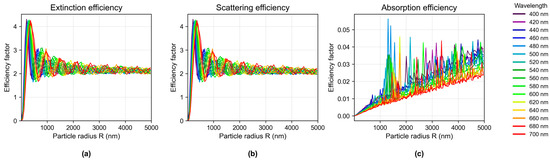
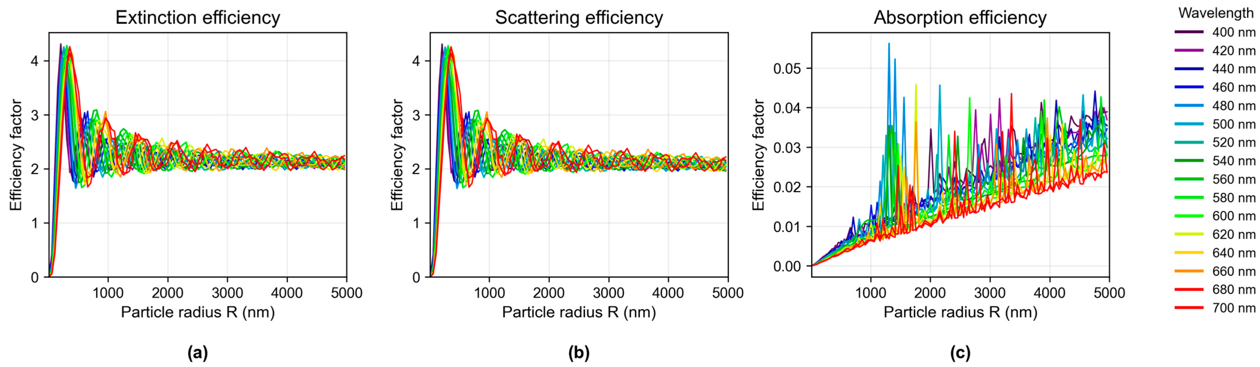
Reference [34] provides the complex refractive index data of water and suspended sediments (represented by silica) in the wavelength range of 400–680 nm. The imaginary part of the refractive index of suspended sediments is on the order of 10⁻⁴. Using the Mie scattering model, the scattering efficiency factor, extinction efficiency factor, absorption efficiency factor, and asymmetry factor of single particles are calculated. The results are shown in Figure 1 for suspended sediments.

Figure 1. Efficiency factors of suspended sediment particles. (a) Extinction efficiency factor; (b) scattering efficiency factor; (c) absorption efficiency factor.

Figure 1 shows the extinction, scattering, and absorption efficiency factors of suspended sediment particles as functions of particle radius at different wavelengths. For small particle radius, the efficiency factors exhibit strong oscillations, which are characteristic of Mie scattering. As particle size increases, the oscillations decrease and the extinction and scattering efficiency factors approach stable values, while the absorption efficiency factor gradually increases. Similar trends are observed for different wavelengths, although the values differ slightly [28].

Based on Mie scattering theory for spherical particles, assuming that particles are uniformly distributed in the water column with a number concentration $N$ and an average radius $r$, the attenuation coefficient $c$ and scattering coefficient $b$ can be expressed as [28]

$$\left\{\begin{array}{c}c\left(\lambda \right)=N{Q}_e\left(\lambda \right)\pi r^2\\ b\left(\lambda \right)=N{Q}_s\left(\lambda \right)\pi r^2\end{array}\right.$$

(4)

In this study, the Henyey–Greenstein (HG) phase function is adopted to describe the relationship between the scattering angle and random numbers, which improves computational efficiency while maintaining simulation accuracy. The expression is given by

$$HG={\displaystyle \frac{1}{4\pi }}{\displaystyle \frac{1-g^2}{{4\pi \left(1+g^2-2gcos\theta \right)}^{\frac{3}{2}}}}$$

(5)

where $\theta$ is the scattering angle and $g$ is the asymmetry factor. The dimensionless parameter $g$ characterizes the preferential scattering direction of particles in a homogeneous medium and is defined as

$$g={\displaystyle \frac{4}{Q_s{x}^2}}\left[\sum _{n=1}^{n_{max}}{\displaystyle \frac{n\left(n+2\right)}{n+1}}Re\left(a_n{a}_{n+1}^{*}+b_n{b}_{n+1}^{*}\right)+\sum _{n=1}^{n_{max}}{\displaystyle \frac{2n+1}{n\left(n+1\right)}}Re\left(a_n{b}_n^{*}\right)\right]$$

(6)

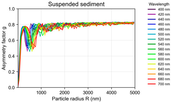
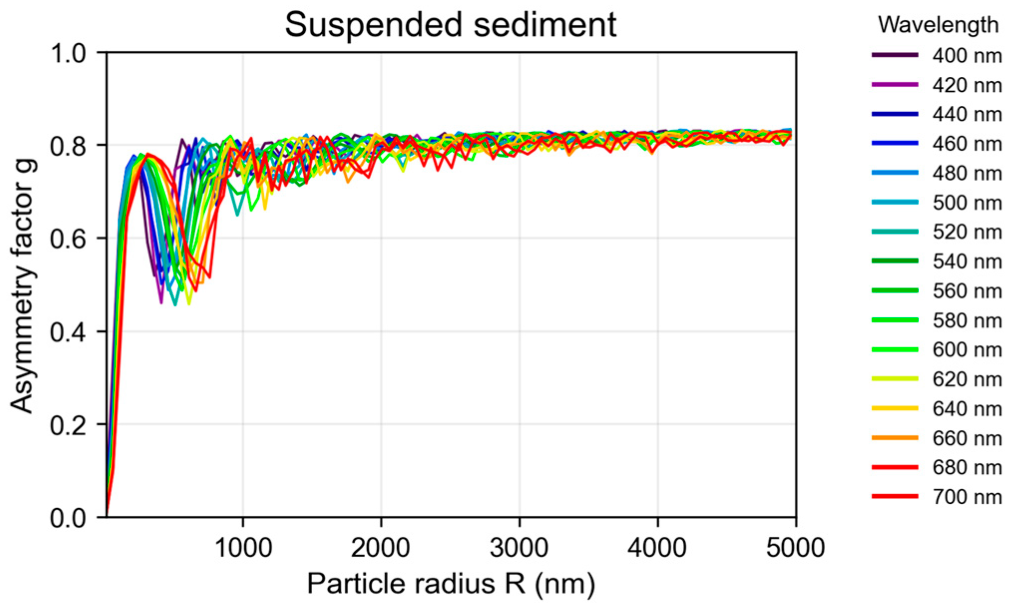
where $a_n^{*}$ and $b_n^{*}$ are the complex conjugates of $a_n$ and $b_n$, respectively. $g$ is a dimensionless parameter that characterizes the anisotropy of scattering. When $g=-1$, scattering is completely backward; when $g=0$, it is isotropic; and when $g=1$, it is entirely forward. Using the refractive index data reported in Ref. [27], the variation of $g$ with particle radius $r$ for suspended sediments is calculated as Figure 2.

Figure 2. Asymmetry factor g.

It can be observed that $g$ exhibits a nonlinear dependence on particle size. When the particle radius R is small, $g$ increases rapidly with noticeable oscillations. As the R further increases, the oscillations gradually decrease and the asymmetry factor approaches a stable value of 0.8. In addition, although similar variation trends are observed for different wavelengths, slight differences appear in the small R range. Previous studies have shown that within the Mie scattering regime, the asymmetry factor is mainly influenced by particle size, while the effect of optical constants such as the complex refractive index is relatively small [21].

2.2. Semi-Analytical Monte Carlo Simulation

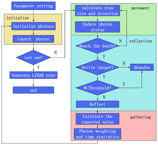
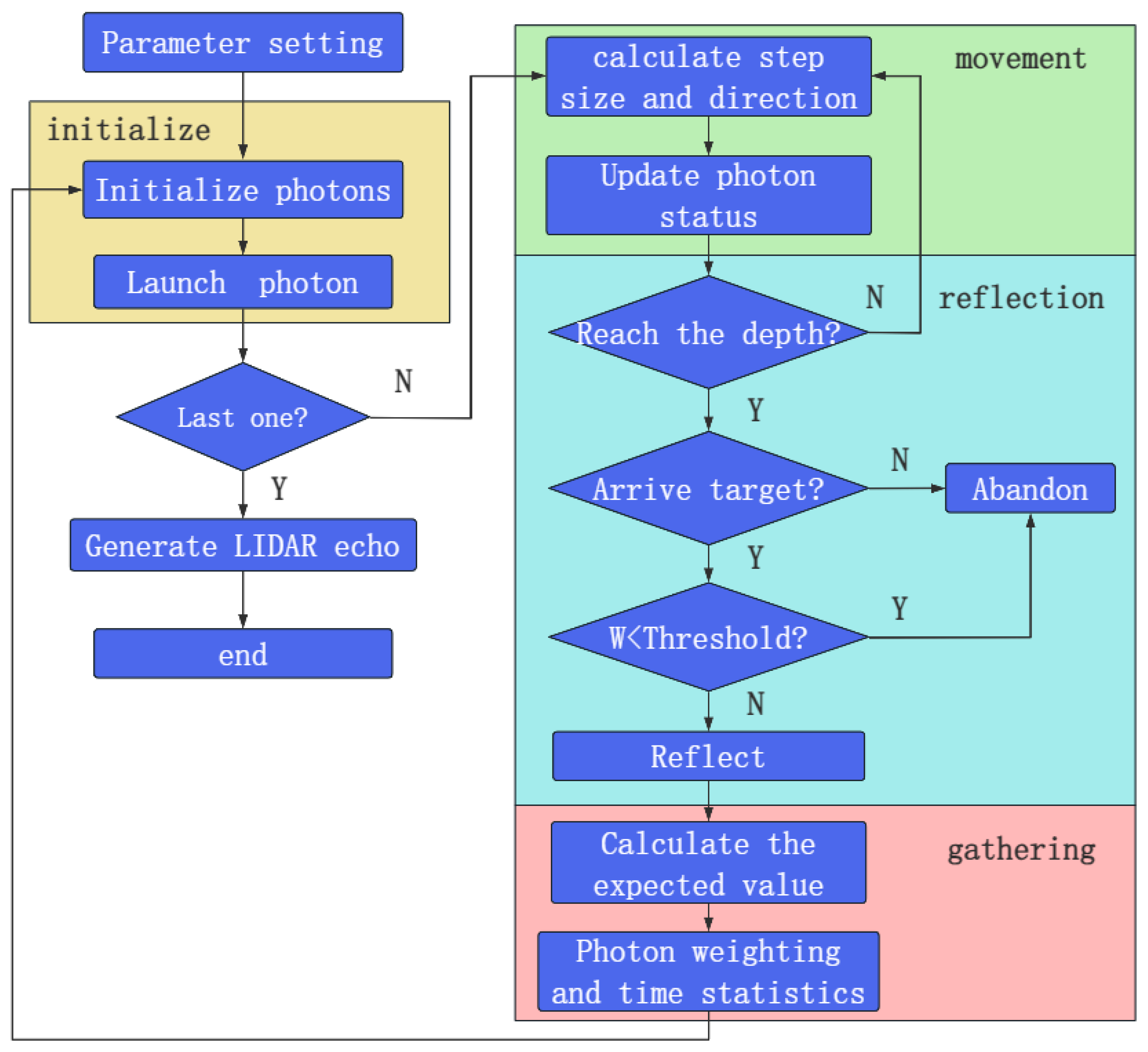
The semi-analytical Monte Carlo model developed in this study for multispectral LiDAR consists of four main modules: the laser emission system, underwater propagation, target interaction, and echo detection. The overall workflow of the model is illustrated in Figure 3.

Figure 3. Flowchart of Semi-analytical Monte Carlo simulation.

• Photon initialization

Assume that the laser emits a Gaussian laser pulse, which contains both temporal distribution characteristics and spatial distribution characteristics. For the pulse waveform, a Gamma distribution(shape parameter k = 3) is adopted to describe the temporal profile of the emitted laser pulse. $P\left(t\right)=A{\displaystyle \frac{t^2}{{\tau }^2}}·\mathit{exp}\left(-{\displaystyle \frac{t}{\tau }}\right)$, A represents the amplitude, $\tau = T/\mathrm{l}\mathrm{n}3$ is the time scale parameter of the Gamma distribution, $T$ is the full width at half maximum(FWHM). The spatial distribution of the laser pulse refers to the energy distribution in the cross-section perpendicular to the propagation direction. According to the Gaussian intensity distribution $I\left(r\right)={\displaystyle \frac{2P}{\pi {\omega }_0}}\exp \left(-{\displaystyle \frac{2r^2}{{{\omega }_0}^2}}\right)$, the initial position of each photon can be determined as ($r_0$, ${\alpha }_0$). Its expression is given as $r_0={\displaystyle \frac{{\omega }_0}{\sqrt{2}}}\sqrt{-\ln \left(1-{\xi }_1\right)}$ and ${\alpha }_0=2\pi {\xi }_2$. The coordinates of the photon are:

$$\left\{\begin{array}{c}{x}_0=r_{0}cos{\alpha }_0\\ y_0=r_{0}sin{\alpha }_0\\ z_0=0\end{array}\right.$$

(7)

For the photon emission direction in the simulation, it is assumed that the spatial divergence of the laser beam is limited within a half-angle ${\theta }_{laser}$. The polar angle of the photon emission direction relative to the optical axis is denoted as ${\theta }_0$, and the azimuth angle is denoted as ${\phi }_0$, where ${\xi }_3$ represents a random number. The azimuth angle $cos{\theta }_0$ is assumed to be uniformly distributed in the interval [$cos{\theta }_{laser},1$]:

$$\left\{\begin{array}{c}cos{\theta }_0=1-{\xi }_1(1-cos{\theta }_{laser})\\ {\phi }_0=2\pi {\xi }_3\end{array}\right.$$

(8)

2.

Movement of photon

For each photon packet, the absorption, scattering, and attenuation coefficient of the water are required as inputs to determine the free path of photons and the probabilities of scattering and absorption. The free step of a photon traveling from the emission point into the water medium can be sampled according to the Beer–Lambert law. According to geometric relationships, the photon position and weight are updated as: $a\left(\lambda \right)b\left(\lambda \right)c\left(\lambda \right)ss=-{\displaystyle \frac{\ln \left({\xi }_4\right)}{c\left(\lambda \right)}}$

$$\left\{\begin{array}{c}{x}^{\prime }=x+{\mu }_{x}s\\ y^{\prime }=y+{\mu }_{y}s\\ z^{\prime }=z+{\mu }_{z}s\end{array}\right.$$

(9)

$$W_{n+1}=W_n\times {\displaystyle \frac{b\left(\lambda \right)}{c\left(\lambda \right)}}$$

(10)

where W_n and W_n+1 are the photon weights before and after the absorption. The motion of photons is continuously tracked until it is determined whether the photon is terminated. After collision, the change in propagation direction is calculated by sampling the Henyey–Greenstein phase function:

$$\theta =\arccos \left({\displaystyle \frac{1}{2g}}\left(\left(1+g^2\right)-{\left({\displaystyle \frac{1-g^2}{1+g-2g{\xi }_5}}\right)}^2\right)\right)$$

(11)

$$\mathsf{\psi }=2\pi {\xi }_6$$

(12)

where $\mathsf{\psi }$ and $\theta$ is the azimuth angle and scattering angle. The direction is updated as

$$\left\{\begin{array}{c}{{\mu }_x}^{\prime }=\sin \theta ({\mu }_x{\mu }_{z}cos\mathsf{\psi }-{\mu }_y\sin \mathsf{\psi })/\sqrt{1-{{\mu }_z}^2}+{\mu }_x\cos \theta \\ {\mu }_y^{\prime }=\sin \theta ({\mu }_y{\mu }_{z}cos\mathsf{\psi }+{\mu }_x\sin \mathsf{\psi })/\sqrt{1-{{\mu }_z}^2}+{\mu }_y\cos \theta \\ {\mu }_z^{\prime }=-{\displaystyle \frac{\mathrm{s}\mathrm{i}\mathrm{n}\mathsf{\psi }\cos \mathsf{\psi }}{\sqrt{1-{{\mu }_z}^2}}}+{\mu }_z\cos \theta \end{array}\right.$$

(13)

Substituting the updated direction into the previous position update equation yields the new photon position. It is necessary to determine the relationship between the photon z-axis coordinate and the distance S between the emission plane and the target plane. If $z_i=\mathrm{S}$, no correction to the photon state is required. If $z_i>\mathrm{S}$, $s^{\prime }= {\displaystyle \frac{S-z_{i-1}}{{{\mu }_z^{\prime }}_{i-1}}}$, the photon coordinates must be corrected as:

$$\left\{\begin{array}{c}{x}_i=x_{i-1}+{{\mu }_x^{\prime }}_{i-1}{s}^{\prime }\\ y_i=y_{i-1}+{{\mu }_y^{\prime }}_{i-1}{s}^{\prime }\\ z_i=S\end{array}\right.$$

(14)

3.

Target diffuse reflection

This study introduces the influence of the receiver field of view (FOV) on the echo from the target. The proportion of the reflected energy that falls within the receiver FOV is incorporated into the simulation in the form of an expectation value:

$$\Delta W_r=W_{down}\rho \left(\lambda \right)cos{\theta }_i{\displaystyle \frac{{\mathsf{\Omega }}_{FOV}}{\pi }} T_{up}\left(\lambda \right)$$

(15)

where $T_{up}\left(\lambda \right)=\mathrm{e}\mathrm{x}\mathrm{p} [-c(\lambda \left)R\right]$ is the return transmission coefficient, ${\mathsf{\Omega }}_{FOV}$ is the solid angle, and $W_{down}$ is the weight of the photon when it reaches the target. By accumulating all photon weight $\Delta W_r$ arriving at the target plane, the total expected weight of the target-reflected echo received by the detector can be obtained.

4.

LiDAR echo modeling

According to the downward path length $L_{down,i}$ of each photon packet and the return distance S, the round-trip propagation time can be calculated as $t_i=2(L_{down,i}+S)/v$ where $v$ is the speed of light in water. The time axis is divided into several equal-width time windows $\mathrm{b}\mathrm{i}\mathrm{n}=[t_k,t_{k+1}$), and $\Delta W_{r,i}$ is assigned to the corresponding time bin, thereby constructing the temporal waveform of the target echo signal.

3. Results and Discussion

3.1. Simulation and Experimental Parameter Settings

According to Equation (4), the optical parameters of the water are related to the efficiency factors, particle radius, and the number of particles per unit volume. However, in practical applications, the number of particles is difficult to measure directly. Water quality is usually characterized by mass concentration. Therefore, by combining the radius and density of ideal spherical particles, the concentration can be derived as

$$C=\rho N{\displaystyle \frac{4}{3}}\pi r^3$$

(16)

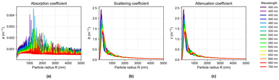
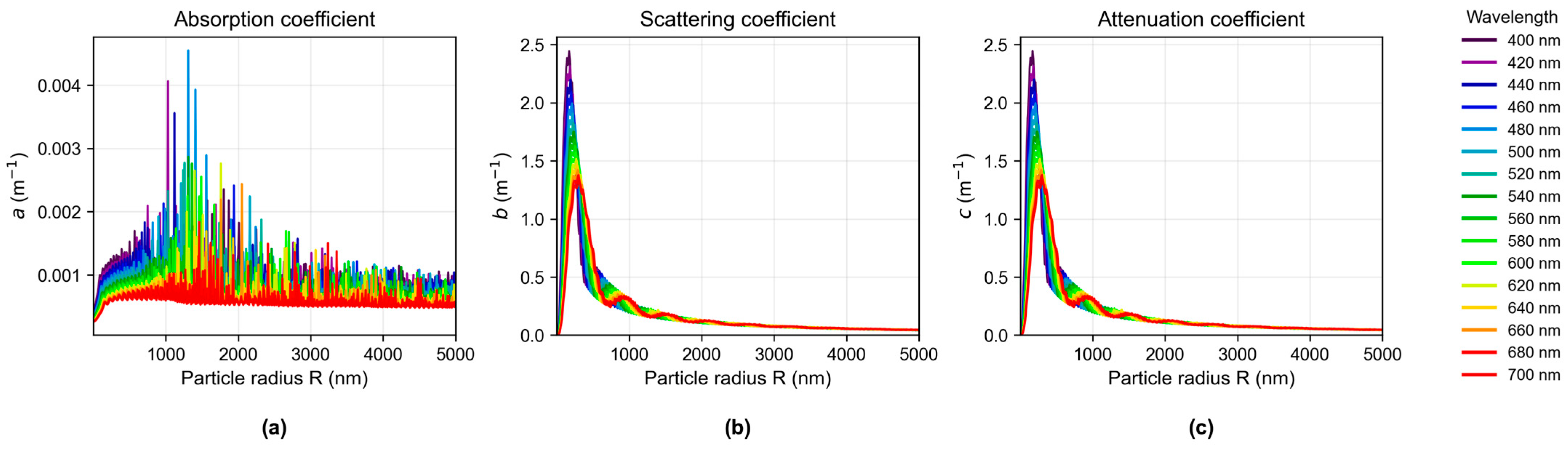
Suspended-particle concentration may vary under different water conditions. For convenience of analysis, according to relevant studies [35], the concentration of suspended sediment particles is set to 1 mg/L. Under this fixed concentration, the variation of optical parameters of water with particle size at different wavelengths can be obtained. Figure 4 shows the optical coefficients of suspended sediments.

Figure 4. Absorption, Scattering and Attenuation coefficient of Suspended sediment. (a) Absorption coefficient; (b) scattering coefficient; (c) attenuation coefficient.

According to the calculated results in Figure 4, the semi-analytical Monte Carlo method described in Section 2.2 is used to simulate the normalized received power under the following parameters. The primary initial parameter settings of the model are listed in Table 2.

Table 2. Initial parameter settings of the Semi-analytical Monte Carlo model.

System Parameters	Characteristic
Laser wavelength	$400-680 \mathrm{n}\mathrm{m}$
Detection distance	$\le 20 \mathrm{m}$
particle radius	100–3000 nm
Initial photon energy weight	1
Number of photons	1 × 10−7
Initial light source position	(0, 0, 0)
Laser divergence angle	$5 \mathrm{m}\mathrm{r}\mathrm{a}\mathrm{d}$
Pulse width (FWHM)	$5 \mathrm{n}\mathrm{s}$
Beam waist radius	$1 \mathrm{c}\mathrm{m}$
Target reflectivity	100% Lambertian reflector
Target diameter	0.5 m
Sampling rate	$10 \mathrm{G}\mathrm{H}\mathrm{z}$
FOV	$1 \mathrm{d}\mathrm{e}\mathrm{g}$

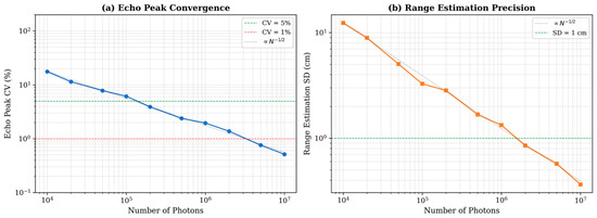
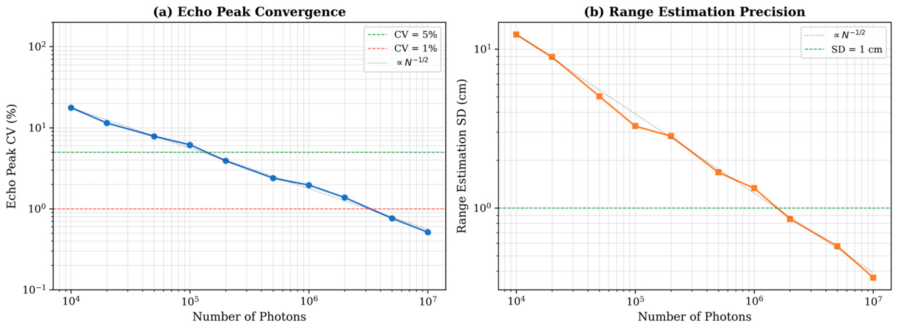
To validate the reliability of the Monte Carlo simulation, a convergence study was conducted by varying the number of simulated photons from 10⁴ to 10⁷. The coefficient of variation (CV) of echo peak intensity decreases from 17.7% at 10⁴ photons to 0.5% at 10⁷ photons, following the expected N^(−1/2) scaling law. The standard deviation of ranging estimates similarly decreases from 0.124 m to 0.004 m. These results confirm that the simulation with 10⁷ photons achieves sufficient statistical convergence for reliable echo and ranging analysis.

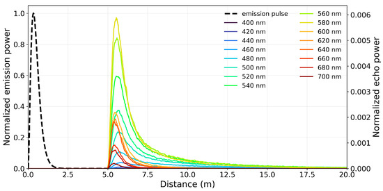
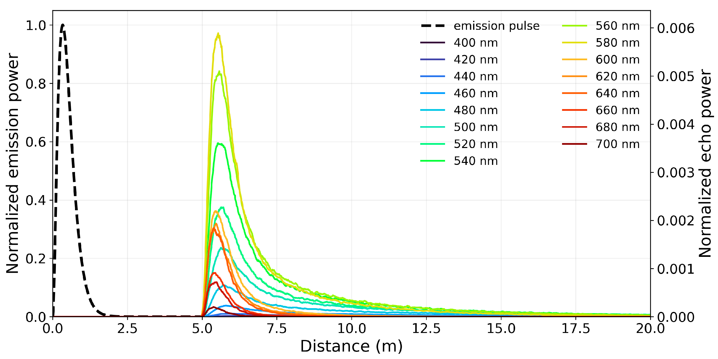
The transmitted pulse waveform is shown in Figure 5. The dashed curve represents the normalized transmitted pulse, and the colored curves represent the normalized received echo signals at different wavelengths.

Figure 5. Monte Carlo convergence study: echo peak coefficient of variation (a) and range standard deviation (b).

To analyze the influence of particle size on the characteristics of the echo waveform, the simulated echo signal is first normalized by dividing it by the peak value of the transmitted pulse. In this way, the received echo waveform represents the relative power distribution of the returned signal with respect to the transmitted energy. Before extracting waveform parameters, a moving-average time window is applied to smooth the echo signal in order to suppress Monte Carlo statistical fluctuations. Figure 6 shows the normalized emission pulse and normalized echo at different wavelengths after processing.

Figure 6. Normalized emission pulse and normalized echo at different wavelengths.

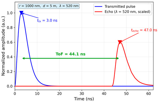
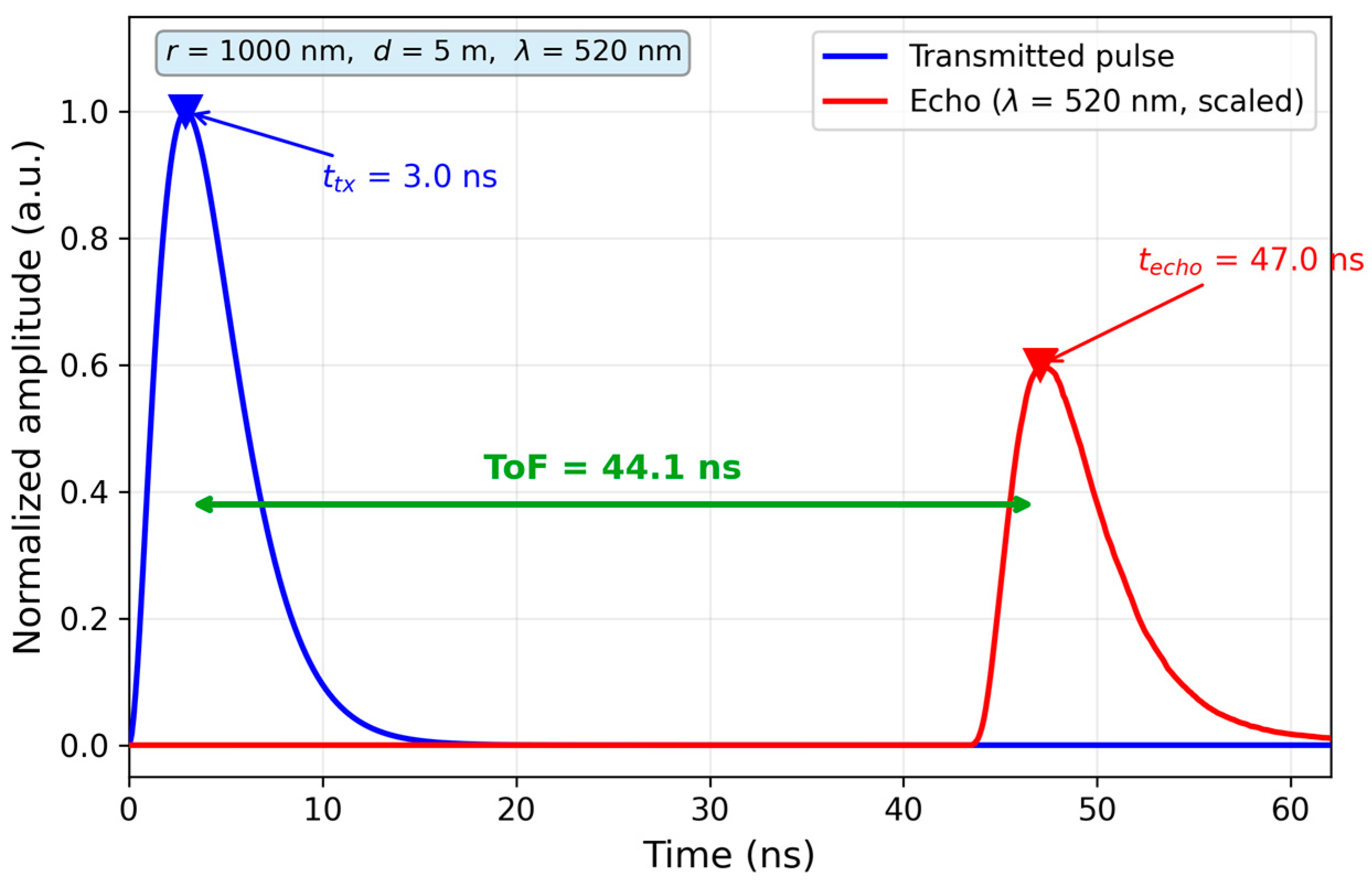
The ranging value in the simulation is determined based on the time-of-flight (ToF) principle. The echo peak time ${\mathrm{t}}_{\mathrm{e}\mathrm{c}\mathrm{h}\mathrm{o}}$ is identified from the maximum of the smoothed echo waveform, and the range is calculated as

$$\mathrm{R}=v_w·({\mathrm{t}}_{\mathrm{e}\mathrm{c}\mathrm{h}\mathrm{o}}-{\mathrm{t}}_{\mathrm{t}\mathrm{x}})/2$$

(17)

where $v_w$ is the speed of light in water (wavelength-dependent due to the Cauchy dispersion model), ${\mathrm{t}}_{\mathrm{t}\mathrm{x}}$ is the transmitted pulse peak time, and the factor of 2 accounts for the round-trip propagation. The ranging error is defined as the difference between the estimated range and the true target distance. Figure 7 illustrates this ToF-based range estimation using a representative simulation result at r = 1000 nm, d = 5 m, and λ = 520 nm, yielding an estimated range of 5.03 m (true distance 5.0 m).

Figure 7. Schematic illustration of the ToF ranging principle.

3.2. Optimal Wavelength Analysis Based on Simulation

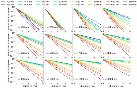
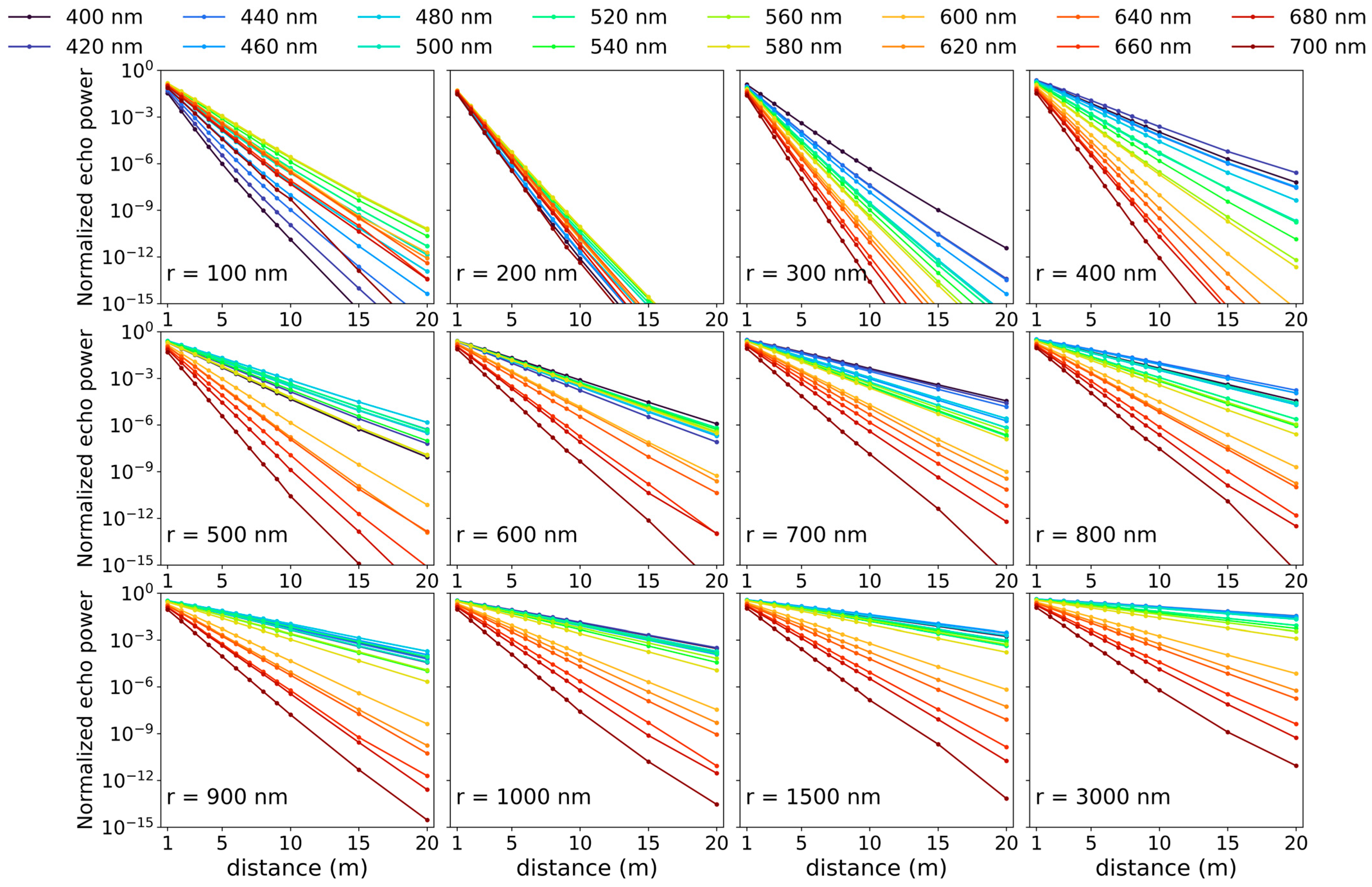
Based on the optical coefficients obtained in the previous section, the distance-dependent attenuation behavior of multispectral LiDAR echo signals at different wavelengths is further analyzed, as shown in Figure 8.

Figure 8. Variation of normalized echo power with propagation distance at different wavelengths under various particle radius.

Overall, under all particle radius and wavelength conditions, the normalized echo power decreases rapidly with increasing propagation distance. This behavior is essentially dominated by the attenuation coefficient determined by the composition of the medium and follows the Beer–Lambert law. It also indicates that the absorption, scattering, and attenuation coefficients of the water body constructed earlier based on Mie scattering theory can be effectively applied in the simulation, demonstrating the consistency between particle-scale optical properties and system-level detection signals.

Particle size has a significant influence on echo intensity. As the particle radius increases from 100 nm to the micrometer scale, the echo power at all wavelengths generally shows an increasing trend, which is particularly evident at short and medium propagation distances. This is mainly because, under a fixed mass concentration, increasing particle size increases the scattering cross-section and scattering efficiency of individual particles, thereby enhancing the contribution of backscattering and increasing the effective echo signal received by the detector.

From the wavelength perspective, the ranking of echo power at different wavelengths varies significantly with particle size. For small particles (100–300 nm), all wavelength curves decay rapidly and remain relatively close to each other. As the particle radius increases, the spectral separation becomes more pronounced, and the blue–green band (approximately 460–560 nm) generally maintains higher normalized echo power over longer distances, whereas the red band attenuates more rapidly. This indicates that the multispectral echo response is jointly controlled by particle size and wavelength, providing the basis for the subsequent threshold screening and optimal wavelength selection.

To provide a quantitative basis for optimal wavelength selection, a detection-threshold-constrained minimum-error criterion is adopted. First, a detection threshold $I_{th}$ is defined as the minimum normalized echo power required for reliable range estimation. For a given particle radius $r$ and propagation distance $d$, only wavelengths whose normalized echo power exceeds this threshold are considered detectable. Among these detectable wavelengths, the optimal wavelength is selected as the one that minimizes the absolute ranging error. This criterion ensures that the selected wavelength provides both sufficient signal strength for detection and the highest ranging accuracy.

$${\lambda }^{*}=argmin |\Delta R(\lambda \left)\right|, subject to I_{echo} \left(\lambda \right) \ge I_{th}$$

(18)

where $\lambda$ is the wavelength, $\Delta R\left(\lambda \right)$ is the ranging error at wavelength $\lambda$, ${\mathrm{I}}_{\mathrm{e}\mathrm{c}\mathrm{h}\mathrm{o}} \left(\mathsf{\lambda }\right)$ is the normalized echo power, and $I_{th}$ is the detection threshold. The constraint ensures that only wavelengths with sufficient echo signal strength are considered, while the objective function selects the wavelength with the highest ranging accuracy among the detectable candidates [36]. In this study, $I_{th}$ is set to 0.1% of the global maximum normalized echo power over all wavelength–radius–distance combinations, corresponding to $I_{th}$ = 3.27 × 10⁻⁴ under the present simulation settings. In real applications, it should be selected based on the emission energy of the lidar system and the sensitivity of the detector.

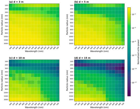
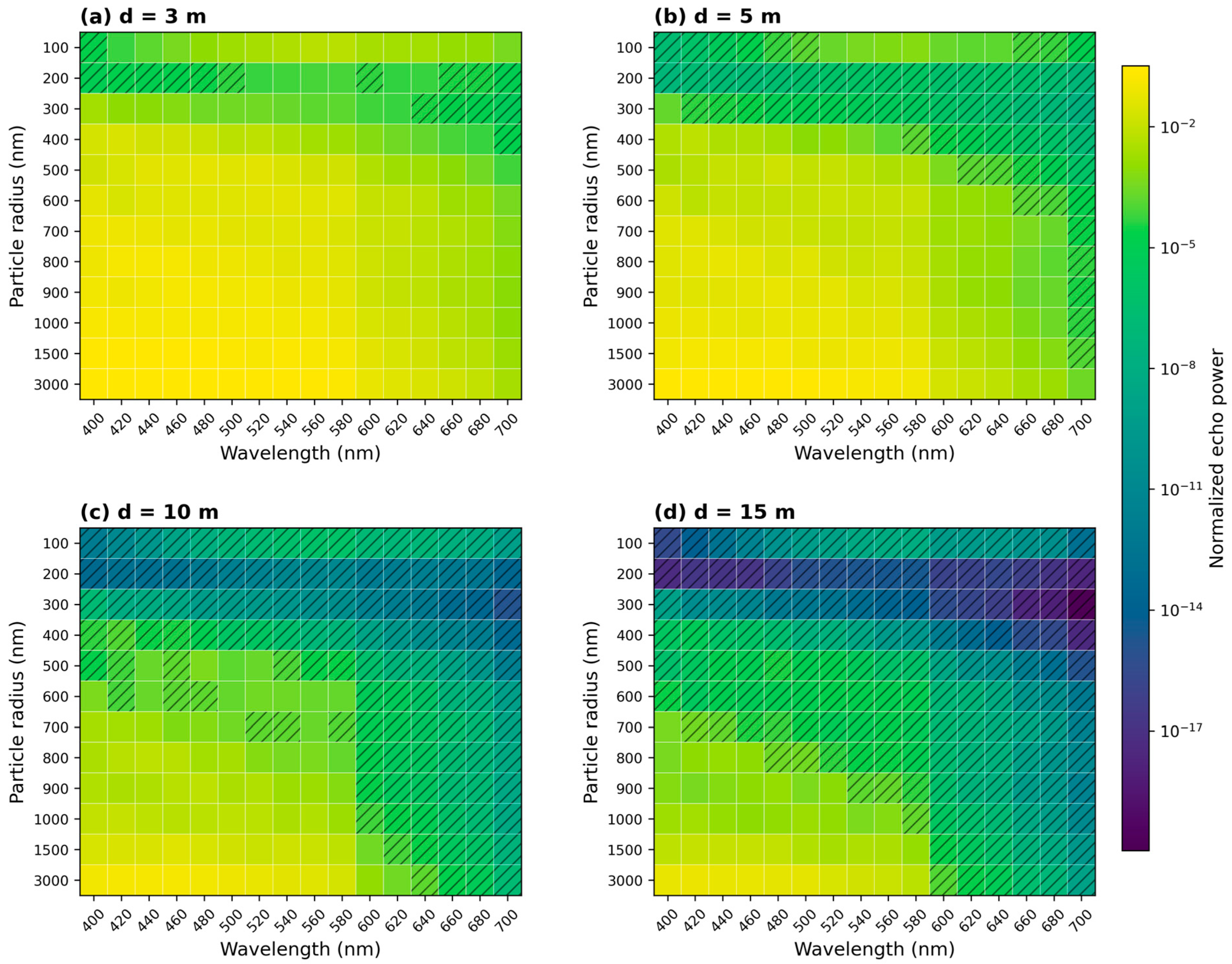
To further examine the detectability of different wavelength–particle-size combinations, the distributions of normalized echo power at four distances are shown in Figure 9. The heatmaps are plotted with wavelength on the horizontal axis and particle radius on the vertical axis for $d=3$, 5, 10, and 15 m. Combinations whose normalized echo power falls below the detection threshold $I_{\mathrm{t}\mathrm{h}}$ are marked by diagonal hatching (///).

Figure 9. Distributions of normalized echo power at four distances: (a) d = 3 m, (b) d = 5 m, (c) d = 10 m, and (d) d = 15 m. Diagonal hatching indicates combinations below the detection threshold.

The heatmaps mainly show the detectable wavelength–particle-size combinations under different propagation distances. As the distance increases from 3 to 15 m, the hatched below-threshold regions expand progressively, indicating a continuous reduction in the detectable candidate set. At 3 m, almost all combinations remain available for subsequent screening. At 5 m, the detectable range begins to shrink, and some fine-particle conditions fall below the threshold. At 10 m, most small-particle combinations are excluded, whereas at 15 m detectable wavelengths are retained only for relatively large particles.

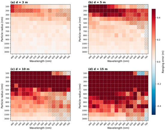
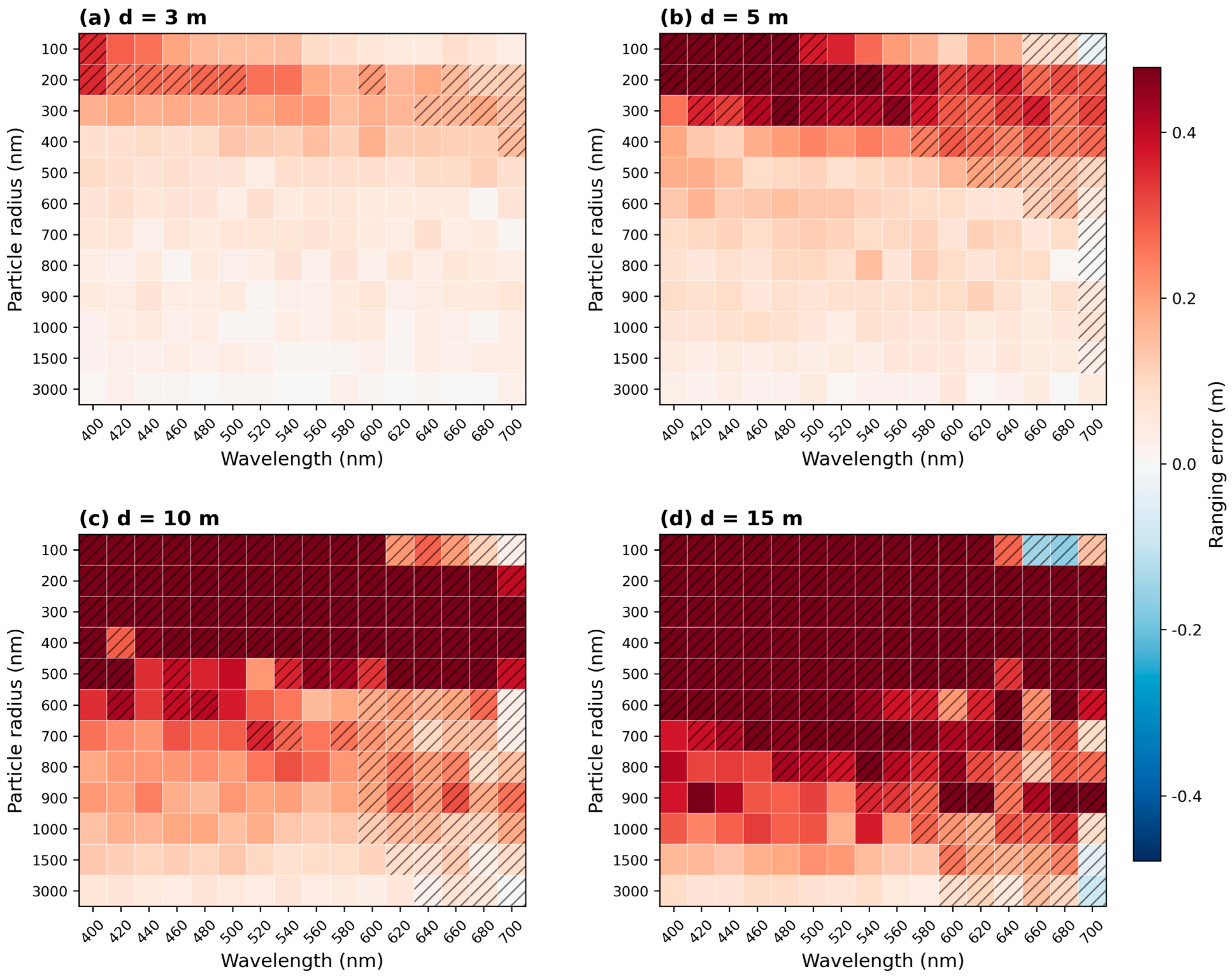
Having established the detectable candidate sets through the echo intensity analysis, the ranging error distributions are next examined. Figure 10 shows the ranging error distributions at the same four propagation distances, with the error defined as the difference between the ToF-estimated range and the true propagation distance.

Figure 10. Distribution of ranging error at four distances: (a) d = 3 m, (b) d = 5 m, (c) d = 10 m, and (d) d = 15 m. Diagonal hatching indicates combinations below the detection threshold.

The heatmaps mainly illustrate the detectable wavelength–particle-size combinations at different propagation distances. As the distance increases from 3 to 15 m, the hatched below-threshold regions expand progressively, indicating a continuous reduction in the detectable candidate set. At 3 m, almost all combinations remain available for subsequent screening. At 5 m, the detectable range begins to shrink, and some fine-particle conditions fall below the threshold. At 10 m, most combinations with small particle radii are excluded, whereas at 15 m only relatively large particles still retain detectable wavelengths. These results define the feasible candidate set for the subsequent optimal wavelength selection. The optimal wavelength λ* and the corresponding minimum absolute ranging error for each particle radius at the four propagation distances are summarized in Table 3.

Table 3. Optimal wavelength ${\lambda }^{*}$ (nm) and corresponding minimum absolute ranging error $\mid \Delta R\left(\lambda \right)\mid$ (m) for different particle radii at four propagation distances.

Particle Radius (nm)	d = 3 m	d = 5 m	d = 10 m	d = 15 m
100	700 (0.036)	600 (0.112)	B/T	B/T
200	580 (0.161)	B/T	B/T	B/T
300	580 (0.149)	400 (0.258)	B/T	B/T
400	400 (0.079)	440 (0.110)	B/T	B/T
500	520 (0.035)	520 (0.077)	520 (0.211)	B/T
600	680 (0.013)	620 (0.067)	560 (0.155)	B/T
700	700 (0.013)	660 (0.055)	440 (0.209)	400 (0.374)
800	460 (0.012)	680 (0.010)	400 (0.185)	420 (0.319)
900	520 (0.012)	660 (0.044)	480 (0.153)	520 (0.231)
1000	500 (0.012)	520 (0.032)	560 (0.121)	520 (0.174)
1500	540 (0.012)	420 (0.030)	540 (0.075)	560 (0.130)
3000	480 (0.000)	680 (0.002)	600 (0.030)	580 (0.039)

Note: Each cell shows λ* (|ΔR| in meters). B/T = below threshold, indicating that no wavelength produced sufficient echo power to exceed the detection threshold at that distance. The threshold is set at 0.1% of the global maximum normalized echo power.

The optimal wavelength varies with both particle radius and propagation distance. However, for particle radii of approximately 500–3000 nm, the selected wavelengths are mainly concentrated in the 400–580 nm range, indicating a relatively stable advantage of this wavelength interval under the present simulation conditions. Although the wavelength-dependent echo-power ranking in Figure 8 remains generally stable with distance, the optimal wavelength in Table 3 changes once the ranging error is considered. This shows that the wavelength associated with the strongest detectable echo is not always the one that yields the highest ranging accuracy. Therefore, the threshold-constrained minimum-error criterion adopted in this study provides a more effective basis for optimal wavelength selection than echo intensity alone.

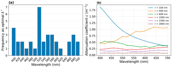
To provide an overall statistical summary of the optimal wavelength selection, Figure 11a counts how often each wavelength is selected as the optimal wavelength ${\lambda }^{*}$ across all detectable particle-radius–distance combinations. The results show that the selected wavelengths are mainly concentrated in the blue–green band, particularly around 480–560 nm, indicating its relatively stable advantage under the present simulation conditions. Figure 11b shows the attenuation coefficient $c\left(\lambda \right)$ for several representative particle radius and provides a qualitative reference for this tendency. In general, the wavelength range with lower attenuation is more likely to remain detectable after propagation and thus has a greater chance of being selected. However, the final optimal wavelength is still determined jointly by the detectability threshold and the ranging error.

Figure 11. (a) Frequency of each wavelength being selected as the optimal λ* across all particle radius–distance combinations; (b) Mie attenuation coefficient c(λ) for representative particle sizes.

Therefore, from the perspective of overall statistical performance, the 400–560 nm band can be regarded as the preferred wavelength range under the current simulation settings. This conclusion should be understood as a model-based trend under simplified assumptions, rather than a universal design rule.

3.3. Experimental Validation

Based on the previous simulation analysis, laboratory experiments were further conducted to provide a preliminary validation of the proposed model under simplified system conditions. First, the experimentally measured laser emission energy spectrum of the laser source is incorporated into the simulation results to reassess the wavelength-dependent echo intensity and to examine whether the previously identified optimal wavelength range remains stable under actual system output conditions. Subsequently, the simulation model was used to analyze and correct the experimental ranging results, so as to evaluate its effectiveness for reducing wavelength-dependent ranging bias under the present laboratory conditions.

3.3.1. Verification of Optimal Wavelength Under Actual Emission Energy Conditions

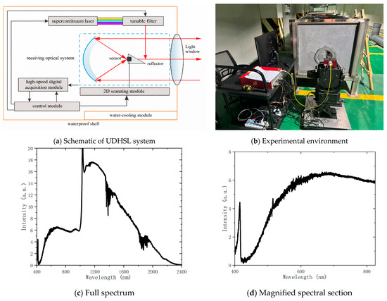
The experimental platform used in this study was an underwater hyperspectral LiDAR system, and its overall structure is shown in Figure 12a [16]. The system mainly consisted of a laser emission module and a receiving optical module. On the transmitter side, a supercontinuum laser combined with a tunable filter was used to achieve flexible wavelength selection and emission within the 450–700 nm spectral range. On the receiver side, target echo signals were collected by the receiving optics, and the full-waveform signals are recorded by a sensor together with a high-speed data acquisition module. This system provided experimental support for analyzing the influence of the actual emission-energy spectrum, preliminarily verifying the wavelength-selection results, and evaluating the simulation-based ranging correction under laboratory conditions. Figure 12b shows the experimental scene, Figure 12c,d show the typical supercontinuum output spectrum of the laser used in this study.

Figure 12. (a) Schematic of UDHSL system, (b) experimental environment, and (c,d) output spectrum of the laser [16].

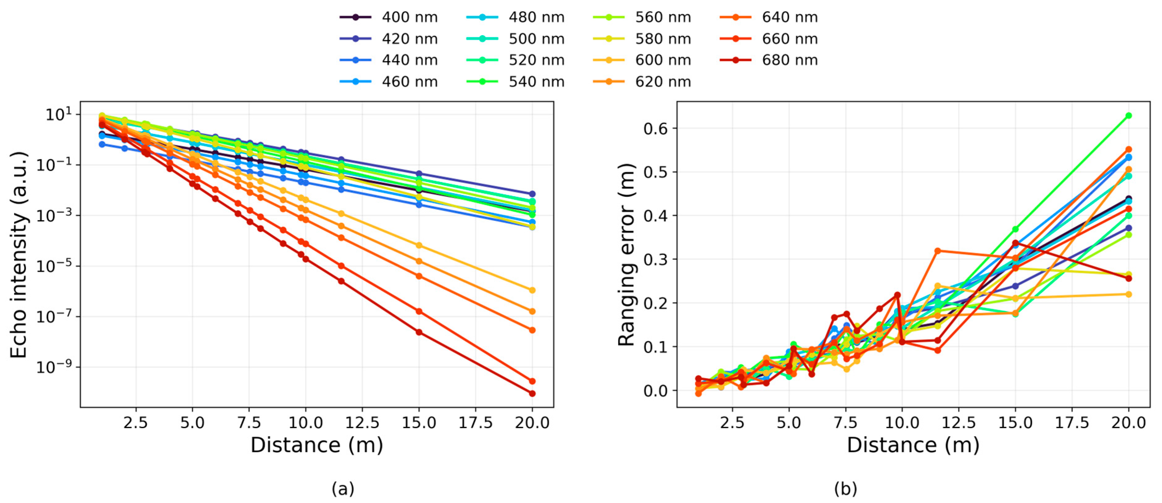
To provide a preliminary laboratory validation of the simulation model under controlled system conditions, experiments were conducted in a laboratory environment using the constructed multispectral LiDAR system. In the experiment, a waterproof Lambertian reflector with a reflectivity of 70% was used as the target, and the echo intensities at different wavelengths were measured at several distances. The experimental water medium was tap water. To approximate the scattering characteristics of the tap water used in the experiment, suspended sediment particles with a particle radius of 1000 nm and a mass concentration of 0.3 mg/L were adopted in the simulation as a simplified equivalent scattering approximation of the water body [37]. This particle setting should be regarded as a preliminary effective-medium assumption for laboratory validation, rather than a full physical description of the actual particle population in tap water or natural waters. The other system parameters were kept consistent with those of the actual multispectral LiDAR system. After incorporating the measured laser emission energy spectrum, the corresponding simulated echo-intensity and ranging-error results are shown in Figure 13.

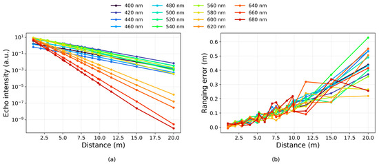
Figure 13. Echo intensity and ranging error. (a) Echo intensity and (b) ranging error.

As shown in Figure 13a, the echo intensity at different wavelengths decreases markedly with increasing distance and remains approximately linear under logarithmic coordinates, indicating that the propagation trend is still mainly governed by medium attenuation. After incorporating the measured emission-energy spectrum, the 620–680 nm bands exhibit relatively enhanced echo intensity at short distances, but this advantage gradually weakens with increasing distance because of their stronger attenuation in water. At longer distances, only part of the 500–580 nm range still maintains relatively high echo levels, indicating that the actual emission-energy distribution affects the short-range spectral response but does not fundamentally change the overall attenuation trend.

Figure 13b shows that the ranging error generally increases with distance for all wavelengths, and the dispersion among wavelengths becomes more pronounced at medium and long distances. Compared with the 500–580 nm bands, the 640–680 nm bands exhibit larger fluctuations at longer distances, which is consistent with their faster echo attenuation and reduced signal quality. Overall, the results indicate that incorporating the actual emission-energy spectrum changes the relative short-range echo response, while the wavelength-dependent ranging performance at longer distances is still mainly constrained by underwater attenuation.

Based on the detection-threshold-constrained minimum-error criterion defined in Section 3.2, the optimal wavelength at each distance was further determined by selecting the wavelength with the minimum absolute ranging error among the detectable candidates. The corresponding results are summarized in Table 4. Overall, the optimal wavelength varies with distance, but it remains mainly concentrated in the 500–580 nm range under the present laboratory conditions. This result suggests that incorporating the actual emission-energy spectrum does not fundamentally overturn the wavelength-selection trend obtained from the simulation but instead provides a preliminary system-level refinement under the present laboratory conditions.

Table 4. Optimal wavelength and minimum absolute ranging error under actual emission energy conditions.

Distance (m)	λ* (|ΔR| in m)
1	420 (0.004)
2	400 (0.007)
3	500 (0.012)
5	520 (0.032)
7	580 (0.074)
9	580 (0.106)
10	560 (0.121)
11.56	580 (0.147)
15	520 (0.174)
20	560 (0.356)

3.3.2. Distance Correction Based on the Simulation Model

For the acquired echo waveform data, peak detection was first applied to determine the positions and amplitudes of the main wave (window-glass echo) and the target echo. The target distance was then estimated from the time difference between the two peaks according to the time-of-flight principle. Moreover, waveforms with echo peak values exceeding 95% of the 16-bit digitizer full-scale range (i.e., unsigned peak > 62,000 out of 65,535 counts) were considered saturated and were discarded [16].

To verify the effectiveness of the established underwater optical propagation model for compensating ranging errors, the ranging errors obtained from the simulation were applied to correct the experimental ranging data. Let the experimentally measured target distance be $R_{exp}$, and the system error calculated by the simulation model be $e_{sim}$. The corrected ranging result can then be expressed as $R_{corr}=R_{exp}-e_{sim}$, where $e_{sim}$ is the systematic ranging deviation caused by the optical propagation characteristics of the water medium. This error is obtained through Monte Carlo photon transport simulations. By introducing this compensation term, the systematic error in the experimental ranging results can be effectively corrected. This correction procedure is mainly used to provide a preliminary assessment of the practical relevance of the model, rather than to establish a universal correction framework for underwater LiDAR measurements.

To quantitatively evaluate the correction performance, the root mean square error (RMSE) and the mean absolute error (MAE) were adopted as evaluation metrics for ranging accuracy. RMSE reflects the overall level of ranging error, while MAE describes the average ranging deviation.

$$\mathrm{R}\mathrm{M}\mathrm{S}\mathrm{E}=\sqrt{{\displaystyle \frac{1 }{N}}\sum _{i=1}^N{(R_i-R_{true})}^2}$$

(19)

$$\mathrm{M}\mathrm{A}\mathrm{E}={\displaystyle \frac{1 }{N}}\sum _{i=1}^N|R_i-R_{true}|$$

(20)

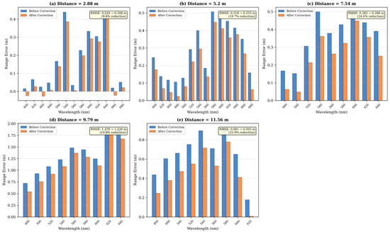
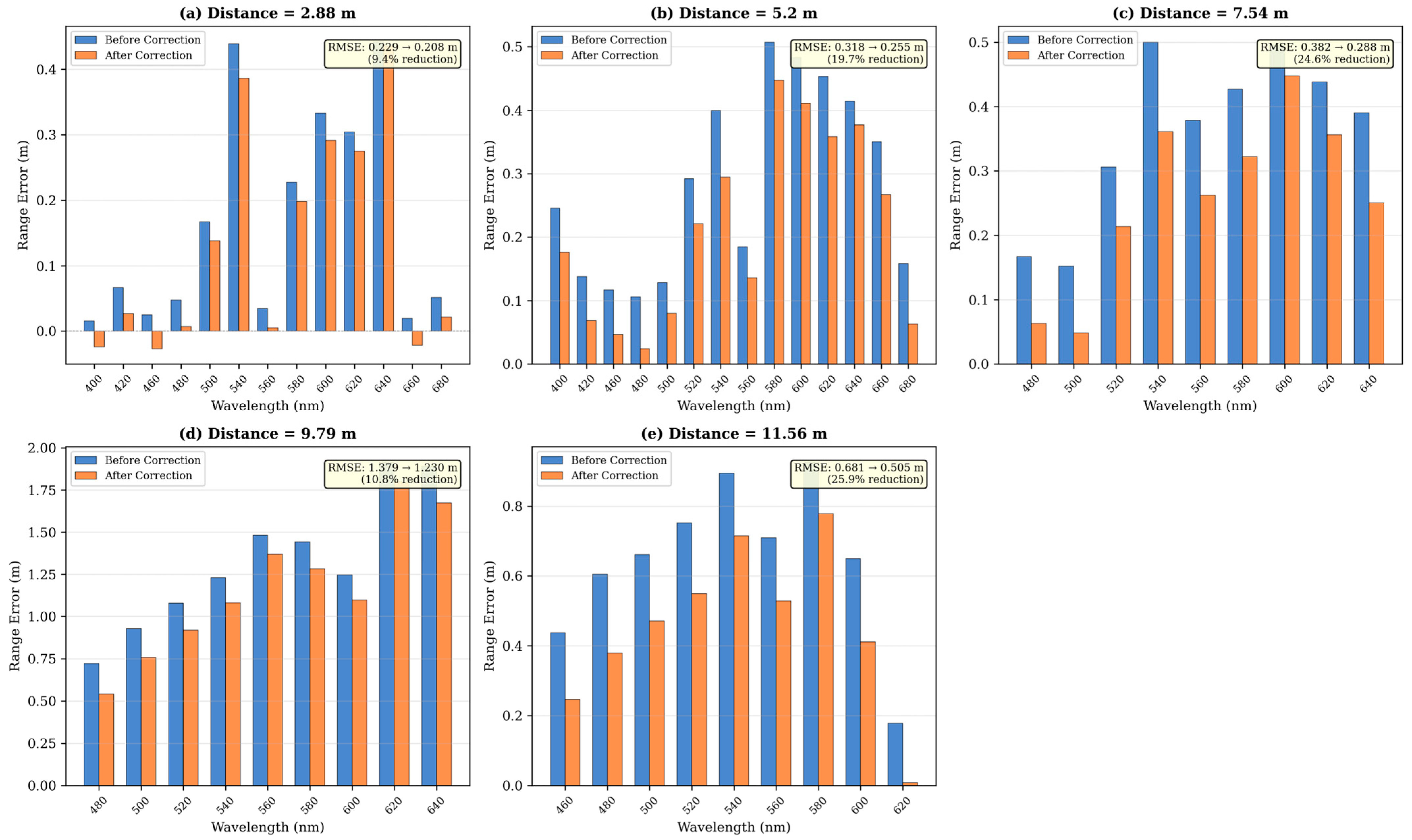
where $R_i$ is the measured distance under the i-th wavelength condition, $R_{true}$ is the true distance, and N is the number of wavelengths involved in the statistics. To verify the effectiveness of this method, all five available experimental distances (2.88 m, 5.20 m, 7.54 m, 9.79 m, and 11.56 m) were used to compare the experimental ranging errors before and after simulation-based correction. Figure 14 shows the wavelength-resolved correction results at each distance, where the ranging error at each wavelength before and after applying the simulation-based correction is compared.

Figure 14. Wavelength-resolved ranging correction at five experimental distances. Blue bars: range error before correction; orange bars: range error after simulation-based correction.

Table 5 presents the quantitative correction results for all five experimental distances. The simulation-based correction reduces RMSE by 9.4–25.9% (average 18.1%) and MAE by 11.8–29.7% (average 22.0%). The correction is effective across all distances, with the largest improvement observed at the intermediate distances (5.20 m and 7.54 m), where optical propagation effects are most pronounced relative to other error sources.

Table 5. Simulation-based ranging correction performance across five experimental distances.

Distance (m)	RMSE Before (m)	RMSE After (m)	Reduction (%)	MAE Before (m)	MAE After (m)	MAE Reduction (%)
2.88	0.229	0.208	9.4	0.167	0.143	14.6
5.20	0.318	0.255	19.7	0.284	0.212	25.3
7.54	0.382	0.288	24.6	0.362	0.258	28.6
9.79	1.379	1.230	10.8	1.325	1.168	11.8
11.56	0.681	0.505	25.9	0.646	0.454	29.7

Overall, the simulation-based correction yields consistent error reduction across all five tested distances, indicating that the proposed underwater propagation model can partially capture the wavelength-dependent ranging bias caused by optical propagation effects. The correction performance varies with distance, with relatively greater improvement observed at intermediate distances, where the simulated optical effects account for a larger proportion of the total ranging error. These results provide preliminary experimental support for the practical relevance of the model and suggest that simulation-based correction can serve as a useful auxiliary approach for reducing propagation-related ranging errors under simplified laboratory conditions.

4. Discussion

This study is subject to several limitations. First, the simulation adopts an equivalent spherical-particle assumption with a monodisperse size distribution and fixed mass concentration. This simplification is useful for analyzing the general effects of particle size on multispectral echo intensity, attenuation, and ranging error, but it cannot fully represent natural waters, where suspended particles are typically polydisperse, irregular in shape, and mixed in composition. Therefore, the present results should be interpreted as trend-level conclusions under simplified conditions.

Second, the experimental validation was conducted under controlled laboratory conditions using tap water rather than real seawater. In the simulation, the laboratory medium was approximated by a simplified equivalent particle setting with a radius of 1000 nm and a concentration of 0.3 mg/L. This treatment should be regarded as a preliminary effective-medium approximation for validation, rather than a full physical description of the actual particle population in tap water or natural waters. Accordingly, the experimental results mainly support the applicability of the model under simplified laboratory conditions.

Third, the proposed correction targets only the ranging bias associated with optical propagation effects, including wavelength-dependent absorption and scattering in water. In practical multispectral LiDAR measurements, total ranging error also contains contributions from instrumental bias, electronic timing delay, detector response, and calibration uncertainty. Since these factors are not included in the present model, the correction should be understood as a physics-based compensation for propagation-induced error rather than a complete correction of all ranging uncertainties.

Future work should extend the model to more realistic particle populations, incorporate additional system-level error sources, and conduct validation in natural waters with different optical conditions. These efforts would help improve the applicability of the present framework to practical underwater multispectral LiDAR measurements.

5. Conclusions

This study addresses how suspended particles under simplified conditions influence multispectral laser propagation and detection performance. By combining Mie scattering theory with the Monte Carlo method, a simplified underwater propagation simulation model for multispectral LiDAR was established, linking particle-scale scattering properties with echo responses. Based on the scattering efficiency, extinction efficiency, and asymmetry factor of suspended particles in the visible band, the absorption, scattering, and attenuation coefficients of the water body were further derived, providing a theoretical framework for analyzing general trends of multi-wavelength laser propagation under idealized conditions.

The simulation results show that particle size has a pronounced influence on multispectral laser propagation under fixed concentration conditions. Under the same mass concentration, increasing particle size enhances the contribution of backscattering and generally increases the received echo signal. The echo signals at different wavelengths decrease approximately exponentially with propagation distance, consistent with the Beer–Lambert law, which supports the physical reasonableness of the proposed model. A convergence study further indicates that the simulation with 10⁷ photons provides statistically stable results for the present analysis (echo CV < 1%, range SD < 0.01 m).

The multi-distance analysis (3, 5, 10, and 15 m) shows that the optimal wavelength is jointly affected by particle size, echo detectability, and ranging accuracy. On this basis, a detection-threshold-constrained minimum-error criterion was introduced for optimal wavelength selection. The results indicate that the optimal wavelength is not fixed, but varies with particle size under the present simulation settings. For particle radii of 100–300 nm, the preferred wavelength is generally concentrated near 560 nm, whereas for particle radii of 500–3000 nm, the preferred wavelength is more often found in the 400–480 nm range. Statistical results from all detectable particle-size and distance combinations suggest that the 400–560 nm band is a relatively favorable wavelength range under the current simplified simulation settings. After incorporating the measured emission-energy spectrum of the actual laser source, the wavelength preference is further adjusted by the source output characteristics, while the 500–580 nm band still shows comparatively stable performance over extended distances.

Preliminary laboratory validation at five distances (2.88–11.56 m) shows that the simulation-based ranging correction can reduce RMSE by 9.4–25.9% (average 18.1%) and MAE by 11.8–29.7% (average 22.0%). These results suggest that the proposed model can describe part of the wavelength-dependent ranging bias caused by underwater optical propagation under the present laboratory conditions and may provide useful support for subsequent ranging-error analysis and correction.

It should be noted that this study still has several limitations, including the equivalent spherical-particle assumption, monodisperse size distribution, simplified concentration setting, and laboratory-only validation in tap water. Therefore, the conclusions should be interpreted as trend-level results obtained under controlled and simplified conditions, rather than as universal rules applicable to all natural waters or operational systems.

Overall, this study provides a simplified but physically grounded framework for analyzing multispectral underwater laser propagation and offers a preliminary reference for wavelength selection and simulation-assisted ranging-error correction in multispectral LiDAR systems under controlled conditions.

References

- Pastra, A.; Johansson, T.M.; Soares, J.; Muller-Karger, F.E. The Use of Emerging Autonomous Technologies for Ocean Monitoring: Insights and Legal Challenges. Front. Mar. Sci. 2025, 12, 1561737. [Google Scholar] [CrossRef] [Scilit]
- Qiao, J.; Yu, J.; Huang, Y.; Feng, H.; Jia, D.; Wang, Z.; Wang, B. AUVs for Seabed Surveying: A Comprehensive Review of Side-Scan Sonar-Based Target Detection. J. Mar. Sci. Eng. 2026, 14, 145. [Google Scholar] [CrossRef] [Scilit]
- Tian, F.; Qin, M.; Lv, N.; Zhao, H.; Nan, Z.; Tao, W. Review of Underwater Laser Imaging Technologies. Opt. Laser Technol. 2025, 192, 113987. [Google Scholar] [CrossRef] [Scilit]
- Woodhouse, I.H.; Nichol, C.; Sinclair, P.; Jack, J.; Morsdorf, F.; Malthus, T.J.; Patenaude, G. A Multispectral Canopy LiDAR Demonstrator Project. IEEE Geosci. Remote Sens. Lett. 2011, 8, 839–843. [Google Scholar] [CrossRef] [Scilit]
- Wallace, A.M.; McCarthy, A.; Nichol, C.J.; Ren, X.; Morak, S.; Martinez-Ramirez, D.; Woodhouse, I.H.; Buller, G.S. Design and Evaluation of Multispectral LiDAR for the Recovery of Arboreal Parameters. IEEE Trans. Geosci. Remote Sens. 2014, 52, 4942–4954. [Google Scholar] [CrossRef] [Scilit]
- Kaasalainen, S.; Nevalainen, O.; Hakala, T.; Anttila, K. Incidence Angle Dependency of Leaf Vegetation Indices from Hyperspectral Lidar Measurements. Photogramm. Fernerkund. Geoinform 2016, 2016, 75–84. [Google Scholar] [CrossRef] [Scilit]
- Sun, H.; Wang, Z.; Chen, Y.; Tian, W.; He, W.; Wu, H.; Zhang, H.; Tang, L.; Jiang, C.; Jia, J.; et al. Preliminary Verification of Hyperspectral LiDAR Covering VIS-NIR-SWIR Used for Objects Classification. Eur. J. Remote Sens. 2022, 55, 291–303. [Google Scholar] [CrossRef] [Scilit]
- Gong, W.; Shi, S.; Chen, B.; Song, S.; Niu, Z.; Wang, C.; Guan, H.; Li, W.; Gao, S.; Lin, Y.; et al. Development and prospect of hyperspectral LiDAR for earth observation. Natl. Remote Sens. Bull. 2021, 25, 501–513. [Google Scholar] [CrossRef] [Scilit]
- Bi, K.; Niu, Z.; Gao, S.; Xiao, S.; Pei, J.; Zhang, C.; Huang, N. Simultaneous Extraction of Plant 3-D Biochemical and Structural Parameters Using Hyperspectral LiDAR. IEEE Geosci. Remote Sens. Lett. 2022, 19, 5501105. [Google Scholar] [CrossRef] [Scilit]
- Bai, J.; Niu, Z.; Wang, L. A Theoretical Demonstration on the Independence of Distance and Incidence Angle Effects for Small-Footprint Hyperspectral LiDAR: Basic Physical Concepts. Remote Sens. Environ. 2024, 315, 114452. [Google Scholar] [CrossRef] [Scilit]
- Bai, J.; Niu, Z.; Huang, Y.; Bi, K.; Fu, Y.; Gao, S.; Wu, M.; Wang, L. Full-Waveform Hyperspectral LiDAR Data Decomposition via Ranking Central Locations of Natural Target Echoes (Rclonte) at Different Wavelengths. Remote Sens. Environ. 2024, 310, 114227. [Google Scholar] [CrossRef] [Scilit]
- Ødegård, Ø.; Mogstad, A.A.; Johnsen, G.; Sørensen, A.J.; Ludvigsen, M. Underwater Hyperspectral Imaging: A New Tool for Marine Archaeology. Appl. Opt. 2018, 57, 3214. [Google Scholar] [CrossRef] [Scilit]
- Mogstad, A.A.; Johnsen, G.; Ludvigsen, M. Shallow-Water Habitat Mapping Using Underwater Hyperspectral Imaging from an Unmanned Surface Vehicle: A Pilot Study. Remote Sens. 2019, 11, 685. [Google Scholar] [CrossRef] [Scilit]
- Dumke, I.; Ludvigsen, M.; Ellefmo, S.L.; Soreide, F.; Johnsen, G.; Murton, B.J. Underwater Hyperspectral Imaging Using a Stationary Platform in the Trans-Atlantic Geotraverse Hydrothermal Field. IEEE Trans. Geosci. Remote Sens. 2019, 57, 2947–2962. [Google Scholar] [CrossRef] [Scilit]
- Du, L.; Wan, D.; Meng, X.; Li, W.; Liang, G.; Li, H. Classification of Underwater Sediments in Lab Based on LiDAR Full-Waveform Data. J. Mar. Sci. Eng. 2025, 13, 624. [Google Scholar] [CrossRef] [Scilit]
- Zhang, H.; Chen, L.; Wu, H.; Zhou, M.; Chen, J.; Chen, Z.; Hu, J.; Chen, Y.; Wang, J.; Niu, Y.; et al. Hyperspectral LiDAR for Subsea Exploration: System Design and Performance Evaluation. Electronics 2025, 14, 1539. [Google Scholar] [CrossRef] [Scilit]
- Ma, Y.; Zhang, H.; Wang, R.; Li, F.; He, T.; Liu, B.; Wang, Y.; Han, F. Underwater Sphere Classification Using AOTF-Based Multispectral LiDAR. Photonics 2025, 12, 998. [Google Scholar] [CrossRef] [Scilit]
- He, Y.; Liu, Y.; Liu, C.; Li, D. Analysis of Transmission Depth and Photon Number in Monte Carlo Simulation for Underwater Laser Transmission. Remote Sens. 2022, 14, 2565. [Google Scholar] [CrossRef] [Scilit]
- Arnush, D. Underwater Light-Beam Propagation in the Small-Angle-Scattering Approximation. J. Opt. Soc. Am. JOSA 1972, 62, 1109–1111. [Google Scholar] [CrossRef] [Scilit]
- Jaruwatanadilok, S. Underwater Wireless Optical Communication Channel Modeling and Performance Evaluation Using Vector Radiative Transfer Theory. IEEE J. Select. Areas Commun. 2008, 26, 1620–1627. [Google Scholar] [CrossRef] [Scilit]
- Schippnick, P.F. Phenomenological Model of Beam Spreading in Ocean Water. In Proceedings of the Ocean Optics X; SPIE: Bellingham, WA, USA, 1990; Volume 1302, pp. 13–37. [Google Scholar]
- Guo, S.; He, Y.; Chen, Y.; Chen, W.; Chen, Q.; Huang, Y. Monte Carlo Simulation with Experimental Research about Underwater Transmission and Imaging of Laser. Appl. Sci. 2022, 12, 8959. [Google Scholar] [CrossRef] [Scilit]
- He, H.; Liu, Q.; Tang, J.; Zhu, P.; Chen, S.; Song, X.; Wu, S. Validation of the Polarized Monte Carlo Model of Shipborne Oceanic Lidar Returns. Opt. Express 2023, 31, 43250–43268. [Google Scholar] [CrossRef] [Scilit]
- Hao, X.; He, Y.; He, H.; Lv, D.; Ruan, Y.; Qi, H.; Xu, G.; Tang, J. Underwater 3D Target Detection: Semi-Analytic Monte Carlo Model and UAV-Based Scanning Lidar System. J. Eur. Opt. Society-Rapid Publ. 2026, 22, 6. [Google Scholar] [CrossRef] [Scilit]
- Huang, Y.; He, Y.; Zhu, X.; Xu, G.; Zhang, C. Semi-Analytical Monte Carlo Simulation of Underwater Target Echoes from a Small UAV-Based Oceanic Lidar. Opt. Commun. 2025, 574, 131157. [Google Scholar] [CrossRef] [Scilit]
- Wang, Z.; Yang, Y.; Shen, X.; Kong, W.; Huang, G.; Shu, R. Multi-Spectral Underwater Lidar Evaluation Based on Semi-Analytical Monte Carlo Methods. J. Opt. Soc. Am. A 2025, 42, 824. [Google Scholar] [CrossRef] [Scilit] [PubMed]
- Zhou, G.; Li, C.; Zhang, D.; Liu, D.; Zhou, X.; Zhan, J. Overview of Underwater Transmission Characteristics of Oceanic LiDAR. IEEE J. Sel. Top. Appl. Earth Observ. Remote Sens. 2021, 14, 8144–8159. [Google Scholar] [CrossRef] [Scilit]
- Gui, D.; Meng, H.; Yang, H.; Liu, X.; Yan, F. Numerical Simulation of Gaussian Laser Beam Propagation Characteristics in Seawater Based on Mie Scattering Model. Laser Optoelectron. Prog. 2024, 61, 0901001. [Google Scholar] [CrossRef] [Scilit]
- Shangguan, M.; Guo, Y.; Liao, Z.; Lee, Z. Discrepancies between Time-Based and Real Depth Profiles in Ocean Lidar Due to Multiple Scattering. Remote Sens. Environ. 2025, 329, 114910. [Google Scholar] [CrossRef] [Scilit]
- Dong, R.; Fang, X.; Meng, X.; Yang, C.; Li, T. Enhancing Underwater LiDAR Accuracy Through a Multi-Scattering Model for Pulsed Laser Echoes. Remote Sens. 2025, 17, 2251. [Google Scholar] [CrossRef] [Scilit]
- Shangguan, M.; Liao, Z.; Guo, Y.; Lee, Z. Seabed Backscattered Signal Peak Shift and Broadening Induced by Multiple Scattering in Bathymetric Lidar. IEEE Trans. Geosci. Remote Sens. 2025, 63, 5701214. [Google Scholar] [CrossRef] [Scilit]
- Chen, Y.; Cui, X.; Gu, Q.; Zhou, Y.; Zhao, H.; Zhang, H.; Ma, S.; Xu, P.; Frielinghaus, H.; Wu, L.; et al. This Is MATE: A Multiple scAttering correcTion rEtrieval Algorithm for Accurate Lidar Profiling of Seawater Optical Properties. Remote Sens. Environ. 2024, 307, 114166. [Google Scholar] [CrossRef] [Scilit]
- Li, X.; Zhang, S.; Chen, P.; Zhang, Z.; Pan, D. IHMSC: A Novel Iterative Hybrid Multiple Scattering-Corrected Retrieval Method for Enhancing Accuracy in Ocean Lidar Profiling Inversions. Remote Sens. Environ. 2026, 334, 115209. [Google Scholar] [CrossRef] [Scilit]
- Polyanskiy, M.N. Refractiveindex.Info Database of Optical Constants. Sci. Data 2024, 11, 94. [Google Scholar] [CrossRef] [Scilit]
- Gupta, M. Analysis of Pre- and Post-Monsoon Suspended Sediments in the Gulf of Kachchh, India Using Remote Sensing. arXiv 2015, arXiv:1503.08369. [Google Scholar] [CrossRef] [Scilit]
- Zhang, Z.; Chen, P.; Mao, Z. SOLS: An Open-Source Spaceborne Oceanic Lidar Simulator. Remote Sens. 2022, 14, 1849. [Google Scholar] [CrossRef] [Scilit]
- GB 5749-2022; National Disease Control and Prevention Administration Standards for Drinking Water Quality. Standards Press of China: Beijing, China, 2022.
Disclaimer/Publisher’s Note: The statements, opinions and data contained in all publications are solely those of the individual author(s) and contributor(s) and not of MDPI and/or the editor(s). MDPI and/or the editor(s) disclaim responsibility for any injury to people or property resulting from any ideas, methods, instructions or products referred to in the content. |
© 2026 by the authors. Licensee MDPI, Basel, Switzerland. This article is an open access article distributed under the terms and conditions of the Creative Commons Attribution (CC BY) license.