


Abstract
Free-space optical (FSO) communication is an attractive high-capacity wireless technology for terrestrial, aerial, and satellite links. However, FSO performance is strongly affected by multiple impairments, including path loss, turbulence attenuation, pointing errors, and equipment loss. Therefore, accurate performance evaluation requires channel modelling that accounts for both deterministic power losses and stochastic channel effects. This paper presents a comprehensive and structured review of FSO channel modelling, covering the transmission, propagation medium, and receiver sections. The composite channel response is represented using a mathematical formulation. Commonly used FSO models are reviewed and organised, including Beer–Lambert and geometrical loss, Kim and Kruse path loss models, Lognormal, Gamma–Gamma, K, and Málaga distributions, along with pointing-error and angle-of-arrival models. Each model is explained in terms of its physical meaning, assumptions, and applicable operating conditions. Lastly, a numerical example is presented to demonstrate how deterministic losses and stochastic channel effects can be combined in FSO performance evaluation.
1. Introduction
Modern communication technologies, including beyond-5G, artificial intelligence, and the Internet of Things, require communication systems that support high data rates, strong security, and low latency. FSO communication transmits optical waves through free space without optical fibres and is a viable solution to meet these requirements. FSO can be deployed across a wide range of space–air–ground and non-terrestrial communication networks. Such links can be integrated with multiple platforms, including unmanned aerial vehicles (UAVs), high-altitude platforms, airships, and satellites [1]. However, FSO systems have important limitations, particularly the strict requirement for line-of-sight (LoS) links. The FSO performance also degrades severely under adverse atmospheric and alignment conditions [2,3]. Fog, smoke, and haze mainly impair the optical beam through absorption and scattering, which reduce the received signal power. By contrast, atmospheric turbulence is caused by random fluctuations in the refractive index of air and mainly introduces wavefront distortion, scintillation, beam wander, and irradiance fluctuations, which can significantly degrade detection performance and link reliability [4,5]. In addition, pointing error (PE) caused by misalignment and jitter between the transmitter and receiver can further reduce the collected optical power.
To analyse and predict FSO system performance under such conditions, a wide range of channel models has been developed and formulated mathematically. These models are characterised by physical mechanisms that affect the propagation of optical waves. In general, FSO models can be classified into two categories: deterministic and stochastic. Deterministic models describe the channel using fixed physical parameters under the assumption of a structured and predictable environment. Examples include the Beer–Lambert law, which characterises optical beam absorption, and the geometrical path loss (PL) model, which accounts for beam spreading. On the other hand, stochastic models describe random channel variations caused by environmental uncertainty. These models are commonly analysed using statistical probability density functions (PDFs) and Monte Carlo simulations. Statistical PDF-based models are widely used to characterise irradiance fluctuations in FSO systems, particularly in outdoor environments. The statistical PDF-based turbulence attenuation (TA) models include the Lognormal, Gamma–Gamma (GG), K, and Málaga distributions (M), each of which is suitable under different turbulence conditions. Moreover, PE models are used to characterise random misalignment between the transmitted beam and the receiver aperture, which may arise from platform vibration, tracking inaccuracy, beam wander, or building sway. Common PE models include the geometric spread, Hoyt, Rician, and Beckmann models.
Although several review and survey papers have discussed FSO propagation impairments and channel models, most of them primarily catalogue individual models or compare them within separate impairment categories. The main distinction of this review is its unified modelling and interpretation perspective. Rather than treating path loss, turbulence attenuation, pointing error, and equipment-related losses as isolated topics, this paper explains how these deterministic and stochastic impairments can be systematically organised and combined into an end-to-end FSO channel response from transmitter to receiver.
1.1. Contributions
This paper focuses on the theoretical and modelling aspects of FSO communication systems. The main contributions of this paper are summarised as follows:
- A unified modelling and interpretation framework for the FSO channel response is presented, combining channel impairments into deterministic and stochastic components from transmitter to receiver.
- Commonly used FSO channel models are reviewed and interpreted in terms of their physical meaning, mathematical assumptions, and applicable operating conditions.
- A comparison of turbulence attenuation models is provided to support appropriate model selection for different environments.
- A numerical example is presented to show how the reviewed models can be combined in a practical FSO performance evaluation.
1.2. Paper Organisation
The remainder of this paper is organised as follows. Section 2 reviews related survey and modelling work on FSO channel models. Section 3 presents an overview of FSO channel models and introduces the channel response. Section 4 discusses PL and absorption models. Section 5 reviews TA models based on statistical PDFs. Section 6 presents pointing error (PE) and angle-of-arrival (AoA) models. Section 7 discusses equipment loss. Section 8 provides a performance analysis. A discussion section is presented in Section 9. Finally, Section 10 concludes the paper.
2. Related Work
Several studies have reviewed and compared FSO channel models. For example, Ref. [6] provides a comparative analysis of PDF turbulence models using the Kullback–Leibler Divergence method, while Refs. [7,8] review atmospheric absorption, TA, and PE models. Meanwhile, Ref. [9] classifies TA models by their advantages. In addition, Ref. [10] surveys the FSO keywords, challenges and mathematical models across the existing literature.
Although existing survey papers have reviewed and compared FSO channel models, most of them focus primarily on cataloguing available models rather than explaining their physical roles within a unified channel framework. In particular, prior reviews often treat path loss, turbulence attenuation, and pointing error as separate topics, while providing limited guidance on how to interpret, select, and combine these components in system-level performance evaluation. To address this gap, this paper organises FSO channel models according to their physical meaning, modelling role, deterministic loss contribution, and stochastic fading behaviour. It also presents a composite statistical formulation of the FSO channel. This perspective helps clarify not only the mathematical structure of different models, but also the assumptions behind them, their appropriate operating conditions, and the situations in which they may become less accurate or less informative.
3. System Overview of Channel Models and Responses
FSO systems operate within the optical spectrum. Practical communication links commonly use wavelengths of 850, 1300, and 1550 nm [11]. As the optical wave propagates through the channel towards the receiving aperture, it experiences both deterministic and random impairments arising from PL, TA, and PE. These impairments can degrade the received power, signal quality, and reliability. Therefore, several channel models must be incorporated to evaluate FSO performance under different channel and operational conditions. Accordingly, the overall FSO channel response, h, adapted from [12], can be expressed as
where represents the PL component, denotes the TA model, accounts for PE, and models the equipment-related losses.
Figure 1 presents the unified end-to-end interpretation of the FSO channel considered in this review. Before reaching the receiver aperture, the transmitted optical signal is affected by deterministic impairments, namely equipment loss and PL, as well as stochastic impairments, including TA and PE. Equipment loss originates from the transceiver hardware, whereas the free-space channel introduces PL and TA, while PE results from imperfect alignment between the transmitter and receiver. This conceptual structure motivates the composite channel formulation adopted in this paper, which represents these effects within a single framework for system performance evaluation. Rather than introducing a new PL, TA, or PE model, this framework provides a structured way to interpret and combine published channel impairments consistently in FSO performance analysis.
Figure 1.
Conceptual diagram of the end-to-end FSO link.
The PL models () depend primarily on the propagation distance, which is often the dominant factor under typical conditions. For example, the geometrical PL, Mie scattering, and Kim and Kruse models are distance-related. These models are often used in FSO link budget analysis to determine the link margin, which represents the minimum received power required for reliable operation.
The TA models () are important for evaluating FSO performance. TA causes random fluctuations in the received irradiance, significantly affecting link quality. A common example is the mirage observed above a hot asphalt road surface, where temperature variations in the air create refractive index fluctuations that distort the optical wave. Several mathematical models have been widely adopted for outdoor conditions [10], such as GG and M models.
The PE models () are also crucial in FSO performance analysis because of the strict LoS requirement. PE arises from building sway, platform movement, mechanical vibrations, or imperfect beam alignment. These effects can be modelled using Rayleigh, Hoyt, Rician, and Beckmann distributions [13,14]. PE can be modelled either as a deterministic pointing loss with a fixed margin or a random pointing loss characterised by a PDF, depending on the model. In addition, AoA fluctuations are another form of pointing-related fluctuation, particularly relevant to UAVs and satellite communication links. AoA fluctuations generally occur when the angle of arrival surpasses the receiver’s field-of-view limit [15]. Although PE can significantly degrade FSO system performance due to random pointing losses, this effect can be mitigated by well-designed pointing, acquisition, and tracking (PAT) systems. Meanwhile, adaptive optics can compensate for PE impairment and turbulence-induced distortion by using a wavefront sensor, control processor, and deformable mirror to reduce distortions [16]. Through such sophisticated engineering solutions, the combination of PAT and AO can improve link availability under severe turbulence, while maintaining alignment and meeting the LoS requirement.
The system loss model () represents the losses in the transceiver, such as laser coupling loss, photodiode responsivity, and thermal noise. Unlike the other losses, system losses arise from hardware components. To address these losses, various techniques, such as system gain optimisation and proper design, have been developed. Other optical power reductions, such as optical background noise, may also be incorporated into this term.
Figure 2 shows the degradation of optical power in an FSO link. In stages I and V, the signal experiences power loss due to hardware components. As the optical signal propagates through free space in stages II and III, additional loss occurs due to PL and TA. However, in stage III, the TA model cannot be directly mapped onto a fixed attenuation value. Instead, it is usually expressed as an outage probability because the received signal fluctuates randomly under varying atmospheric conditions. Therefore, the grey area at stage III represents the range of possible optical power levels caused by these random fluctuations while still maintaining the overall concept of power degradation. At the receiver in stage IV, further degradation may occur from PE impairment. The grey area at stage IV represents the received optical power affected by misalignment. However, this effect may be mitigated in practice through modern engineering solutions rather than being fully neglected. To sum up, the received optical power is determined by the cumulative effects of equipment loss, path loss, turbulence attenuation, and pointing error, where deterministic losses appear as fixed reductions and stochastic impairments appear as ranges of possible power levels.
Figure 2.
FSO power level versus propagation stage.
It should be noted that and are deterministic scaling factors related to fixed power losses , whereas and are random channel variables characterised by PDFs. Consequently, the overall channel response combines deterministic link margin effects with stochastic fading processes. Since originates from refractive index fluctuations, while is related to beam misalignment caused by jitter and boresight displacement, the two effects are assumed to be statistically independent in order to obtain a tractable composite channel model. Under this assumption, the average received optical power can be expressed as
where is the received optical power, is the transmitted optical power, and is the statistical expectation operator. This equation shows that the deterministic losses and directly scale the mean received power, whereas the stochastic effects of TA and PE affect it through their statistical averages.
The composite PDF can be derived by first writing the overall channel response (h) conditioned on the turbulence state (), and then averaging this conditional distribution over all possible turbulence states through the turbulence PDF. The composite PDF of the atmospheric optical channel for the overall channel response h, including both TA and PE effects, is given by [17]:
where is the conditional PDF of h given , and is the turbulence attenuation PDF. Although this equation does not explicitly show the PE term , this term is already included in the overall channel response in Equation (1). When the channel response is conditioned on the turbulence state , and and are treated as deterministic constants, the remaining random contribution is represented by . Therefore, the conditional PDF is obtained by a simple change of variable from the PE PDF , which result in
Substituting Equation (4) into Equation (3), the unconditional composite PDF becomes
This equation separates the deterministic link-margin factors ( and ) from the stochastic components ( and ), enabling any combination of TA and PE models to be substituted into Equation (5) for system performance evaluation.
4. Path Loss Models
As the transmitted FSO signal propagates through the medium toward the receiving aperture, it encounters numerous environmental particles, including dust, ash, soil, smoke, soot, and chemical aerosols. These particulates scatter and absorb optical energy, gradually reducing signal intensity along the propagation path. The received optical power, known as irradiance, can be described using PL models.
4.1. Beer–Lambert’s Law
The Beer–Lambert law provides a simple model for specifying the attenuation or absorption coefficient () of the medium, which quantifies the rate of attenuation per unit propagation distance. It is expressed as
where I is the received irradiance (), is the transmitted irradiance (), and L is the optical path length through the medium in meters. This model forms the fundamental basis for PL estimation in FSO systems.
4.2. Geometrical Path Loss
As the beam propagates, it spreads out, causing a reduction in its intensity [18]. Figure 3 shows the geometrical spreading of an optical beam in free space. At the Rayleigh range, the beam diameter becomes , meaning that the beam area has doubled and the wavefront radius of curvature reaches its minimum. The geometrical path loss depends on the propagation distance (L) in meters, the transmitter aperture diameter () in meters, the receiver aperture () in meters, and the beam divergence angle (). As increases, the beam spreads more, which leads to greater geometrical path loss. In an ideal case, approaches zero, so the geometrical path loss becomes very small.
Figure 3.
Geometrical spreading of a Gaussian optical beam in free space [18].
The geometrical PL model is determined by the following equation [19]:
where is the beam divergence (mrad), is the transmitter gain, and is the wavelength (nm). According to the geometric PL model (Equation (7)), as the link distance increases, the beam spreads further, resulting in a reduction in the received optical intensity.
Figure 4 shows the geometric PL for optical beams at wavelengths of 850, 1300, and 1550 nm with cm over different propagation distances. The 1550 nm beam remains above the 1300 nm and 850 nm beams across all distances. This occurs because beam divergence increases with wavelength. A longer wavelength produces a wider beam spread. Therefore, based on the geometrical PL model, lower wavelengths experience less geometric spreading loss than higher wavelengths.
Figure 4.
Geometrical path loss versus propagation distance at 850, 1300, and 1550 nm.
4.3. Kim and Kruse Models
The Kim and Kruse models are based on visibility range information. These models are developed from Mie scattering theory but require only visibility and optical wavelength parameters. The Kim and Kruse PL models can be expressed as [20]
where V is the visibility range (km), is the optical wavelength (nm), and p is the scattering size distribution coefficient associated with the Kim and Kruse models. The wavelength of 550 nm is commonly used as a reference point in the visible spectrum. According to the Kim model, p is given by
According to the Kruse model, p is defined as
However, when visibility is less than 0.5 km, the Kim model yields , indicating that the attenuation becomes independent of the FSO wavelength. This represents a limitation of the Kim model. Consequently, several alternative fog attenuation models have been proposed for low visibility regimes, such as the FASCOD model [21], the general fog model [22], and the RMSE model [23]. Figure 5 shows the fog attenuation models for different PL models under foggy conditions at wavelengths of 850 and 1550 nm.
Figure 5.
Optical intensity loss versus visibility range for five path loss models at (a) 850 nm and (b) 1550 nm.
Figure 5 shows optical intensity loss versus visibility range for several PL models. As visibility decreases, the attenuation increases. In addition, at 1550 nm, the optical loss is lower than at 850 nm for all PL models. Therefore, visibility range is an important parameter for FSO performance analysis. Since visibility is mainly determined by atmospheric conditions, it decreases as fog density increases. An international visibility code has also been established in [24] to classify various weather-related conditions. Based on this concept, Table 1 presents the visibility ranges for various atmospheric conditions.
Table 1.
Visibility range values corresponding to atmospheric conditions.
According to Table 1, rain generally causes lower attenuation than fog because fog reduces visibility more severely than rain. Snow can also cause optical attenuation, with values ranging from 3 to 30 dB/km [25].
FSO PL models are useful for predicting optical intensity loss under different weather conditions. Although many models have been developed, the Kim and Kruse models remain common visibility-based PL models for representing fixed path loss. This is because the Kim and Kruse models primarily depend on the visibility range variable, unlike other models that rely on approximate values under specific conditions.
In this section, PL models are discussed to describe deterministic optical power reduction mechanisms in FSO systems, including the Beer–Lambert law, the geometrical PL model, and the Kim and Kruse models. The Beer–Lambert law characterises the exponential loss caused by absorption in the propagation medium. The geometrical PL model accounts for beam divergence, showing that the optical beam spreads with distance, beam divergence, and wavelength. Meanwhile, the Kim and Kruse models relate the optical power loss to visibility range and wavelength under various weather conditions. The Beer–Lambert law is widely adopted in FSO PL model research because of its simple form, which approximately represents PL parameters and weather conditions through a single attenuation parameter (). However, the combination of the geometrical PL, Kim, and Kruse models is often used because they provide a more detailed description of beam spreading and weather-related path loss in FSO performance analysis.
5. Turbulence Attenuation Models
Optical signals propagate through atmospheric channels under atmospheric conditions that exhibit different levels of turbulence. To understand the behaviour of optical signals, statistical channel models in the form of PDFs have been proposed.
In terrestrial FSO communication, random fluctuations in the atmospheric refractive index caused by variations in temperature and pressure distort the optical wavefront and lead to random fluctuations in the received irradiance. This effect is called scintillation. The scintillation index is typically in the range [0–1]. The scintillation level can be evaluated directly from the received FSO signal. The scintillation value in the range can be expressed as [26]
where is the received optical intensity and denotes the ensemble average. There are three categories of scintillation: weak, moderate, and strong, which correspond to different turbulence levels. Strong scintillation is generally considered when , moderate scintillation when , and weak scintillation when .
The scintillation index (SI) is another measure of TA. It is defined as the normalized difference between the peak and dip values of the received FSO signal power. In practice, the SI is often manually scaled over 15 min intervals by measuring the received optical intensity [27]. The SI can be expressed as
where is the third-largest peak power value (dB) and is the third-deepest dip power value (dB) of the received signal. For digital signals, the index is commonly used to determine the normalized root-mean-square fluctuation of the received signal intensity [28]. The index can be written as [29]
The index usually ranges from 0 (no scintillation) to 1 (strong scintillation). The index can also be classified into weak, moderate, and strong regimes, similar to the scintillation index .
However, the average of the received optical intensity I is difficult to measure directly. Therefore, researchers often use the Rytov approximation variance as a theoretical turbulence strength, which is related to the fluctuation of the refractive index ().
The usually ranges from to [30]. Larger values of indicate stronger turbulence, leading to increased turbulence-induced fading and potential visual blurring, such as the shimmering effect observed when gazing across a sun-heated asphalt road. By contrast, small values cause only mild shimmering rather than severe blurring. Values of between to are considered to correspond to moderate turbulence, whereas values greater than indicate strong turbulence. These values are therefore useful for assessing TA in FSO systems. The index depends on altitude, location, and time. As altitude increases, the index generally decreases and becomes significantly smaller above approximately 10 km altitude. The turbulence strength is typically greatest within the first 1–2 km above the ground. According to this model, the index can be expressed as [18]
- Daytime:
- Nighttime:However, the index also depends on other factors such as geographic location, temperature, and atmospheric pressure. Therefore, relying solely on a parametric model may not be suitable for all situations. In practice, scintillometers, which measure fluctuations in atmospheric temperature, humidity, pressure, and altitude, can provide more reliable data for estimating [31,32].
Returning to the Rytov variance, the index can be used to describe the TA through Rytov variance , given by
where k is the optical wavenumber , L is the link distance in meters, and H is equal to 1.23 and 0.496 for plane waves (flat wavefronts) and spherical waves (curved wavefronts), respectively. The Rytov variance is commonly used to categorise turbulence-induced attenuation as weak (), moderate (), strong (), and saturated turbulence () [33]. However, for very strong turbulence (), the Rytov variance can be approximated as
where H is equal to 0.86 and 2.73 under strong turbulence approximation for plane and spherical waves, respectively.
Figure 6 shows the Rytov variance as a function of propagation distance for three different TA levels defined by the index. As the optical wave propagates through a longer free space path, turbulence effects accumulate. Moreover, larger values correspond to stronger atmospheric turbulence, which leads to more severe fluctuations in the received optical signal. The Rytov variance is an important parameter used in many turbulence models, including in LN, GG, K, NE, I-K, Nakagami-m, Weibull, and Rayleigh TA models [34].
Figure 6.
Rytov variance with different refractive index structure constant.
5.1. Additive White Gaussian Noise
AWGN is a fundamental model used to represent receiver noise. Although it is often included in FSO performance analysis, it is not a turbulence attenuation model. In practical FSO receivers, additive noise arises from sources such as thermal noise, shot noise, and background radiation. Accordingly, in an AWGN channel, the received signal is the sum of the input waveform and a white Gaussian noise term ), which can be expressed as [35]
For FSO systems, the received signal is commonly given by [36]
where is the received electrical signal, is the photodiode responsivity (A/W), is the transmitted optical signal, and is an additive Gaussian noise term. The AWGN model assumes that the channel is linear and the additive noise is statistically independent of the transmitted signal. It provides a simplified analytical framework for evaluating the impact of receiver and environmental noise on system performance. However, AWGN does not describe turbulence-induced fading. In FSO systems, atmospheric turbulence causes multiplicative random fluctuations in the received optical intensity, whereas the AWGN model represents additive noise as an independent random process. These turbulence-induced fluctuations are modelled using statistical PDFs such as the LN, GG, and M models, and are treated separately from additive noise in system analysis.
5.2. Lognormal Model
The LN model is one of the most commonly used TA models for FSO systems. The model is typically applied under weak turbulence conditions (), since it becomes less accurate when irradiance fluctuations become strong. The LN PDF is expressed as [37]
where I is the optical intensity, is the mean value of I, and is the intensity under free-space (no turbulence) conditions.
Figure 7 shows the LN model with and different . As the increases, the PDF becomes more spread out and more skewed, indicating stronger irradiance fluctuations. For the orange line where , the irradiance is likely to be less than the reference point ( or 0 dB). Therefore, as the increases, the peak of irradiance probability tends to decrease. As increases, the PDF becomes broader and its peak shifts towards lower irradiance values. This means that low-irradiance events become more pronounced as turbulence strengthens. As approaches 1, the distribution becomes highly skewed, suggesting that the LN model is nearing the limit of its validity. Therefore, when , the LN model cannot predict the optical intensity under moderate to strong turbulence conditions. Consequently, other TA models have been developed to address this limitation.
Figure 7.
Lognormal PDF under weak turbulence for different Rytov variance values.
5.3. Negative Exponential Model
The NE model is commonly used for saturated turbulence regimes (). Under this condition, the SI approaches 1, meaning that very strong irradiance fluctuations occur. Consequently, the effects of the Rytov variance, aperture diameter, and propagation distance are no longer represented explicitly in the PDF and become less dominant than the strong irradiance fluctuations. The NE PDF can be expressed as [38]
where is the mean irradiance. The NE model is simpler than the LN model, as it is parameterised only by the mean irradiance and does not explicitly include a turbulence parameter . This indicates that, under saturated turbulence conditions, the PDF is characterised mainly by the average received irradiance. Figure 8 shows the NE model for different values of . The graph represents the optical beam under saturated turbulence conditions. As the value increases, the fading becomes less severe, and higher received irradiance levels become more likely. Conversely, lower values of mean stronger fading and lower irradiance. However, since the model depends only on and does not explicitly account for , its application is generally limited to saturated turbulence conditions.
Figure 8.
Negative exponential PDF for different mean irradiance values.
Under saturated turbulence, the NE PDF is highest at and decreases as I increases. This means that low irradiance values occur more frequently than high ones. However, this does not mean that approaches 0, since represents the mean irradiance—that is, the statistical average of the received optical power. Therefore, the FSO link may still operate, but with severe irradiance fluctuations, increased outage probability, and reduced reliability unless mitigation techniques such as diversity, aperture averaging, or relaying are implemented. The NE model is a classical reference model for saturated turbulence. Many subsequent models, such as the GG and I-K distribution models, can reduce to or approximate the NE model under saturated turbulence conditions.
5.4. K Distribution Model
Under very strong turbulence () conditions, the modified K model was proposed as a suitable model [39,40]. The generalized K-distribution is a three-parameter distribution with parameters , , and . The PDF can be expressed as
where is the mean value, is the Gamma function, is a modified Bessel function of the second kind, and the shape parameters are and . The K model, a classical model, is commonly used to model channel fading and shadowing in wireless communications. However, based on FSO experimental data, the K model can be modified by setting , which yields the modified K distribution PDF given by [41]
where is related to the effective number of scatterers. The modified K model is a suitable model for strong turbulence conditions, where Rytov variance lies in the range [42].
Figure 9 shows the effect of the parameter in the modified K model. As the increases, the received irradiance becomes more stable. This indicates weaker turbulence, where deep fades are less likely. Conversely, smaller values of produce a broader distribution with a heavier tail. This implies stronger turbulence effects, where weak irradiance levels occur more frequently because of random fading. Although the parameter is not measured directly in practice, it is usually estimated by fitting the K-distribution to experimentally measured irradiance data. This can limit the practical use of the model, since accurate parameter estimation often requires experimental data or prior channel measurements before a realistic FSO PDF simulation can be performed.
Figure 9.
Modified K distribution for different values.
5.5. Lognormal-Rician Model
To cover weak-to-moderate turbulence conditions, the LR model was proposed [14]. The LR model assumes that the received irradiance is formed by the product of lognormal and Rician components, representing large-scale and small-scale fluctuations, respectively. The model has shown good agreement with experimental data, particularly for spherical waves [43]. The LR PDF is obtained from the product of the Rician and lognormal distribution models, and can be expressed as [44]
where z is a lognormal random variable that represents the large-scale turbulence fluctuation, is the zero-order modified Bessel function of the first kind, r is the empirical coherence parameter of the small-scale Rician component, and is the lognormal distribution variance or strength of the large-scale turbulence fluctuations. The LR model can be reduced to the LN model by assuming . Consequently, the effect of the small-scale Rician component becomes negligible and the model depends only on large-scale lognormal fluctuations.
In Figure 10, the blue line () has the highest PDF in the plotted range, while the purple line () has the lowest. This shows that r and variables affect the shape of the PDF. As r increases, the coherent component becomes stronger, and the small-scale fluctuations become less significant. On the other hand, larger values of indicate stronger large-scale turbulence fluctuations. Therefore, the LR model captures the combined influence of coherence- and turbulence-induced fading on the received optical signal. Compared with the LN model, the LR model provides a more physically flexible description of turbulence, including both large- and small-scale effects, rather than relying solely on the Rytov variance parameter in the LN PDF. However, this advantage comes at the cost of higher mathematical complexity and the need to estimate the empirical parameter r from experimental data. As a result, many researchers have attempted to estimate or simplify the model using methods such as a two-step generalised method of moments, k-nearest neighbour [45], and saddle-point approximation [44].
Figure 10.
Lognormal–Rician PDF for different values of r and .
5.6. Gamma–Gamma Turbulence Attenuation Model
The GG model is widely used to describe the turbulence effects in FSO systems [46]. The GG PDF is derived from the generalized K and LR model by mainly using the to explain the turbulence effects. It can be expressed as [47]
where represents the effective number of large-scale cells in the scattering process, represents the effective number of small-scale eddies, is the Gamma function, and is the modified Bessel function of the second kind. The parameters and can be written as follows
where and are the normalized variances of large-scale and small-scale eddies, respectively. The received irradiance can then be expressed as . Moreover, the SI is given by
Therefore, the parameters of large- and small-scale scintillation for plane waves can be expressed as follows [48,49]:
where Rytov variance for plane waves.
For example, an FSO link operates at 1550 nm over a link distance of m with a receiving aperture diameter mm. The refractive index structure parameter is taken as and to represent various turbulence conditions. The corresponding GG model is shown in Figure 11.
Figure 11.
GG model with different values: (a) plane waves; (b) spherical waves.
In Figure 11, under weak turbulence (), for both plane and spherical waves, the irradiance values cluster tightly around −5 to 5 dB, indicating that only small irradiance fluctuations occur under this condition. As the turbulence becomes stronger—that is, as increases—the irradiance distribution becomes broader and more spread out. This means that the received optical intensity exhibits stronger random fluctuations due to greater refractive index variations in the atmosphere. As a result, the probability of deep fading increases, reducing the stability of the FSO link and degrading its performance. By comparing Figure 11a,b, the spherical wave is slightly less affected by turbulence than the plane wave under the same . This is because the spherical wave has a spreading wavefront, which makes it less sensitive to atmospheric refractive fluctuations and results in weaker scintillation. The GG model captures this behaviour through the parameters and , which vary with turbulence strength and describe the large- and small-scale irradiance fluctuations. Therefore, the GG model is suitable for showing both the effect of increasing and the difference between plane and spherical waves on FSO performance. The parameters of large- and small-scale scintillation for spherical waves can be expressed as [48]
where is the Rytov variance for spherical waves, , , D is the receiver aperture diameter, and L is the link distance.
The GG model primarily relies on the Rytov variance to determine its distribution parameters. This may limit its accuracy outside the Rytov approximation regime, since FSO performance is influenced by other variables such as the aperture diameter, inner scale (), outer scale (), and coherence parameter () [50]. However, the GG model can still be applied under weak-to-strong turbulence conditions. This flexibility has made the GG model one of the most widely used for statistical FSO channel models.
5.7. Málaga Distribution Model
The M model is a general distribution adaptable to different turbulence conditions. Although the model requires additional parameters and is less convenient in practice [51], its expression can be represented in terms of Meijer’s G and Fox’s H functions, which reduces analytical complexity [52]. The M PDF unifies the Rice-Nakagami, LN, K, IK, GG, and the NE models, and can be expressed as [53]
where is a modified Bessel function of the second kind and order , is the Gamma function, is the binomial coefficient, is the fading amount parameter (a natural number), and is a positive parameter related to the effective number of large-scale cells of the scattering process. The effective coherent power and the incoherent scattering power are given by
where is the average power of the LOS component, is a factor that depends on the propagation path length or the coherence parameter, is the average power of the total scatter components, and the operator is the ensemble average.
For example, FSO link performance can be evaluated using the M model by assuming that the optical wave propagates under strong ( and ), moderate ( and ), and weak ( and ) turbulence conditions, with [54]. The resulting FSO PDFs are shown in Figure 12.
Figure 12.
M model with different turbulence conditions.
As the and parameters increase, the PDF peak shifts towards a higher irradiance region. This reflects that the received optical intensity is less affected by random fluctuations, and hence higher irradiance values become more probable under weaker turbulence conditions. Therefore, the figure confirms that the M model can describe the statistical behaviour of the received irradiance across strong-to-weak turbulence conditions using the parameters. The M model can be converted to other general TA PDF models, namely the AWGN, K, and GG models. For example, the model reduces to the K model by assuming , (no coupled-to-LOS scattering power), and (no LOS power). While the model reduces to the GG model by assuming , (full coupled-to-LOS scattering), and (no LOS power). In the asymptotic case where and , the M model approaches the ideal AWGN model, which corresponds to a turbulence-free optical channel. This shows that the M model not only provides a flexible description of irradiance fluctuations, but also offers a unified statistical framework for analysing different atmospheric turbulence regimes in FSO systems. However, the model requires more parameters to be flexible.
This section has reviewed representative statistical PDF models for turbulence attenuation in FSO systems. Most of these models are parameterised by , which characterises the strength of atmospheric turbulence. Each TA model introduces its own set of parameters to describe the statistical fluctuations of the received irradiance under different turbulence conditions. In general, the selection of a TA model involves a trade-off between physical accuracy, mathematical tractability, and parameter availability. For example, the LN model is simple and analytically convenient, but it is mainly suitable for weak turbulence. The NE and K models are specifically appropriate for saturated and very strong turbulence, respectively. The LR model can be adapted to weak-to-moderate turbulence conditions, but at the cost of increased analytical complexity. By contrast, the GG model is widely adopted because it offers a good balance of accuracy, tractability, and applicability across a wide range of turbulence conditions, though it requires more parameters than simpler models. The M model is the most general among these distributions and can represent several classical models as special cases, but its practical use depends on the availability of additional parameter estimates. Therefore, simpler models may be preferred for tractable analysis in specific turbulence conditions, whereas the GG and M models are more suitable when broader applicability and more accurate turbulence characterisation are required. Table 2 summarises the main TA models used for FSO system performance analysis.
Table 2.
Practical selection guidance for common FSO TA PDF models.
It should be emphasised that the PDF-based TA model describes the statistical fluctuations of the received irradiance. These models do not correspond to fixed FSO power loss and therefore cannot be directly mapped onto the fixed attenuation steps shown in Figure 2. Instead, they represent the probability that the received optical power takes different values due to refractive index variations in the atmosphere. These PDFs are used to evaluate performance metrics such as outage probability and BER. Figure 1 serves only as a simplified illustration of how an FSO signal propagates through a medium, whereas turbulence-induced fading must be treated statistically using its PDF model. Other turbulence models also exist in the literature, such as I-K, Exponentiated Weibull (EW), Fisher–Snedecor (F) distribution, Double Gamma Gamma, Nakagami-m distribution, Inverse-Gaussian distribution, and the Rayleigh model. However, this review focuses on the most widely adopted and experimentally validated models.
6. Pointing Error Models
FSO communication requires strict LoS alignment between the transmitter and receiver to enable reliable optical signal transmission. Precise LoS alignment can be achieved through appropriate engineering structures that support accurate point-to-point communication. A lack of precise alignment can lead to misalignment and PE, which reduce the received power and degrade system performance. Such effects often occur due to building sway and earth subsidence. To evaluate the impact of PE, several statistical models have been proposed, such as the geometric spread with Rayleigh [12], Hoyt [55], Rician [56], and Beckmann [57] models.
6.1. Geometric Spread Model
The PE model can be derived under the assumption of a Gaussian beam propagating over a distance . The Gaussian beam radius at the receiver can be approximated from the geometric PL model (Figure 3) as [58]
where is the beam waist at the transmitter (), , is the coherence length, is the refractive index, and is the wavenumber. Consider the detection aperture of radius (a) with the PE length (r) as shown in Figure 13. The approximation of the fraction of power collected by the aperture can be derived as [12]
where is the collected power fraction at , is the equivalent beam width, and is the beam width at the receiver.
Figure 13.
Aperture and beam width at receiver plane [59].
A misalignment of the beam is shown in Figure 13. The smaller circle is the aperture with radius a, while the larger grey circle is the received beam footprint with beam width . The misalignment r represents the distance between the beam centre and the aperture centre. As r increases, the overlap between the beam and the aperture decreases, so less optical power is collected. From Equation (41), the value, which is the normalised mean-squared error (NMSE), is normally used to explain the ratio between the beam width and aperture size. As becomes larger, more of the beam falls outside the aperture, which increases power loss. For an acceptable NMSE value to evaluate this PE model, it should be below , which corresponds to the beam width condition reported in [12]. Therefore, this PE model is suitable for an FSO beam that is not larger than the aperture by a factor of six .
Substituting the power collected fraction with the Rayleigh distribution radial displacement (r), the PE equation for the zero-boresight case (no systematic misalignment) can be expressed as [12]
where is the ratio between the equivalent beam width and standard deviation of the PE displacement (jitter), and is the jitter standard deviation. This model provides a basic analytical framework for describing PE effects in terms of beam width, aperture size, jitter, and propagation distance. The model shows that the collected power statistically depends on the relationship between the beam width and the jitter. As jitter increases, the radial displacement increases, reducing the collected power fraction and increasing the probability of fading. In contrast, a larger equivalent beam width relative to the jitter leads to a less severe PE effect. Therefore, this model is useful for evaluating how misalignment statistically degrades FSO link reliability and received power performance.
6.2. Hoyt Model
Under the geometric spread assumption, the PE is modelled by assuming identical jitter in the vertical and horizontal directions. However, to distinguish the jitter along the horizontal (x) and vertical (y) directions, as shown in Figure 14, the Hoyt model is used to characterise this directional jitter. The Hoyt PDF model can be expressed as [55]
where , , , is the PE displacement standard deviation (jitter), , , is the equivalent beam width, r is the PE length, and is the modified Bessel function of the first kind of order zero. It is worth noting that when , the Hoyt model reduces to the geometric spread model.
Figure 14.
Aperture and beam width with non-identical jitters [60].
Figure 14 shows the beam footprint and receiver aperture under non-identical jitter conditions. The parameters x and y represent the random horizontal and vertical pointing fluctuations. This figure shows a possible instantaneous beam position caused by random jitter along the x and y axes. Such jitter can occur due to earthquakes, unstable transceiver, or wind loading. Therefore, the Hoyt model provides a more flexible representation of asymmetric jitter than the geometric spread model.
6.3. Beckmann Model
The Beckmann model is a flexible pointing-error model that includes several previously proposed models as special cases, including the geometric spread, Hoyt, and Rician models. It is parameterised by and variables. The Beckmann PDF can be expressed as [57,61]
where r is the PE length, and are the jitter standard deviations in the horizontal and vertical directions, and are the effective mean displacements in the horizontal and vertical directions (boresight offsets), , are the PE parameters, and the parameter G is an approximate Beckmann factor. The variables are shown in Figure 15.
Figure 15.
Beam footprint with respect to generalized misalignment and jitter effects.
PE impairment can arise from boresight displacement, represented by and , and random jitter spread, represented by and . The Beckmann model can capture both types of impairment. The model can also be reduced to the previously proposed PE models as special cases, including the geometric spread model by assuming and (identical misalignment and jitter), the Hoyt model by assuming and (identical misalignment and non-identical jitter), and the Rician model by assuming and (non-zero boresight displacement). Therefore, the Beckmann model is a flexible PE model because it includes several previously proposed models as special cases and can represent both jitter asymmetry and boresight displacement.
6.4. Angle of Arrival Model
FSO can be deployed across a wide range of space–air–ground and non-terrestrial communication networks. Such links can be integrated with multiple platforms, including UAVs, high-altitude platforms, airships, and satellites. When these platforms operate under different alignment angles, the FSO transceivers may not remain perfectly aligned, which reduces the effective field of view (FoV) of the receiver aperture. This effect can be called AoA fluctuation. Figure 16 shows an example of AoA fluctuation.
Figure 16.
An example of AoA with misalignment: (a) geometry view; (b) beam footprint.
Figure 16 shows that, when the receiver aperture is not parallel to the transmitter, FoV fluctuation occurs. As the optical signal arrives at the receiver () at angles and , rather than normal to the receiver plane, as shown in Figure 16a, the beam footprint at the receiver is distorted by the AoA impairment. As shown in Figure 16b, the beam footprint becomes distorted due to AoA impairment. Therefore, AoA fluctuation degrades the amount of optical power that can be effectively collected by the receiver. The and are the horizontal and vertical AoA components, respectively. The AoA fluctuation can be expressed as
The Rayleigh PDF is then given by
where is the variance of the independent zero-mean Gaussian AoA components. For a receiver with a finite FoV , the AoA PDF can be approximated as [15]
where is the Dirac delta function.
The PE models describe stochastic misalignment effects that cause random fluctuations in the optical power collected at the receiver aperture. Different PE models offer different characteristics and levels of complexity. The geometric spread model is the simplest and is suitable when identical jitter is assumed in the horizontal and vertical directions with zero boresight displacement. The Hoyt model provides improved realism by allowing non-identical jitter variances in the two directions, although it remains limited to zero-boresight conditions. The Rician model is more suitable when a fixed boresight displacement exists, but it usually assumes identical jitter statistics. By contrast, the Beckmann model offers the most general representation, since it can jointly describe asymmetric jitter and non-zero boresight displacement, and also includes the geometric spread, Hoyt, and Rician models as special cases. AoA fluctuation should be treated separately, since it is associated with FoV variation rather than jitter- or boresight-based PE modelling. Therefore, simpler models are preferable when tractable analysis is required under restricted assumptions, whereas the Beckmann model is more suitable for most practical situations where both jitter asymmetry and boresight displacement occur simultaneously.
7. Equipment and Other Losses
The previous sections reviewed the PL, TA, and PE models. These impairments are treated as channel-related losses. However, there is another type of loss known as hardware loss, which can degrade the laser signal at the transmitter and receiver subsystems [62]. This loss is called equipment loss , which arises from the optical components and interfaces.
7.1. Hardware Losses
At the transmitter, performance is affected by both losses and gains. Transmitter-side losses may arise from imperfect laser coupling, wavelength mismatch, modulation loss, thermal effects, and voltage instability, whereas gain may be improved by increasing the transmitted power or aperture size. Similarly, the receiver is affected by losses such as limited photodetector sensitivity, filter loss, and lens loss. Receiver-side performance can be improved through a larger aperture, signal recovery techniques, and coding. Therefore, the equipment loss can be expressed as [63]
where is the subsystem gain, and is the subsystem loss for the transmitter and receiver. Since equipment loss originates from hardware components, its impact may be reduced through improved subsystem design and overall system optimisation.
7.2. Other Losses
Other noise sources that may degrade FSO performance, such as sunlight [58], beam wavelength selection [61], and quantum noise, should also be considered. Background noise from sunlight scattered and reflected by the sky, clouds, and surrounding objects can cause shot noise at the aperture and reduce the signal-to-noise ratio (SNR), particularly in daytime and outdoor systems. Moreover, wavelength selection may occur when the operating wavelength is poorly matched to the receiver optical filter or the atmospheric transmission window. Furthermore, quantum noise arises from receiver limitations. These losses are commonly treated as additive noise terms and may be included in the equipment loss.
8. Numerical Example of Application Scenarios
This section shows how the reviewed PL, TA, and PE models are combined in an FSO performance evaluation. First, a link budget analysis determines the deterministic power margins under different atmospheric conditions, and the M model is applied to evaluate outage probability without PE. Next, the average bit error rate (BER) and the ergodic Shannon capacity upper bound are evaluated under a composite channel model that includes the Kim path loss, the M, and the geometric spread PE model.
8.1. Link Budget and Outage Probability
The PL channel of the system can be expressed as , where is the geometrical loss and is the Kim model. Calculating from Table 3, , which corresponds to approximately −5 dB, and is −0.45 dB, −1.5 dB, and −15 dB for clear air, rain, and fog conditions, respectively. With a 4 dB equipment loss, the total fixed loss is approximately −9.45 dB (clear air), −10.5 dB (rain), and −24 dB (fog). These numbers represent the link budget of the FSO link when turbulence and misalignment fluctuations are neglected. Hence, the link margins become [64]
where is the receiver sensitivity. Two common photodetector types are PIN and avalanche photodiode (APD) receivers. Their sensitivities are −28 dBm and −35 dBm, respectively. Table 3 summarises the FSO parameters under different weather scenarios. In this example, the FSO system is evaluated using the geometrical, Kim, and Málaga models without PE fluctuations.
Table 3.
System and environmental parameters for the FSO link.
In this scenario, only the PIN diode is considered. Consequently, the link margins are 28.55 dB, 27.5 dB, and 14 dB, for clear air, rain, and fog conditions, respectively. Figure 17 shows the optical power loss at each stage of the channel response.
Figure 17.
Optical power level at each stage of the FSO link under clear air, rain, and fog conditions.
Figure 17 shows the optical power in an FSO link under clear air, rain, and fog conditions. Starting from the transmitted power, all cases experience the same reduction due to geometrical spreading (). Additional attenuation then occurs at the atmospheric stage through (), where fog causes significantly greater power reduction than rain and clear air. Then, the expected received power after turbulence effects shows the impact of random fluctuations caused by TA without PE impairment. Finally, equipment loss () introduces an additional deterministic power reduction at the receiver.
The M model is then used to evaluate the outage probability performance, using the parameter values shown in Table 4.
Table 4.
Parameters of the M model.
For the IM/DD receiver with a PIN photodiode, the outage probability is evaluated at a target electrical SNR threshold . The outage probability can be expressed as
In the following results, is the average electrical SNR parameter of the IM/DD receiver, while the link budget analysis is used separately to interpret the operating conditions under clear air, rain, and fog scenarios. Therefore, the instantaneous electrical SNR in linear scale for the IM/DD model can be expressed as
As a result,
In Figure 18, the outage probability decreases as the average SNR increases for all turbulence conditions. Among the three weather cases, fog exhibits the highest outage probability and therefore requires the highest average SNR to achieve acceptable link availability. To achieve a link availability, corresponding to an outage probability of , the required average SNR under fog conditions is approximately 70 dB. This requirement is very high and may be impractical for typical FSO system configurations.
Figure 18.
Outage probability under the Malaga turbulence model without PE.
Based on the link budget analysis, the transmitted optical power is 10 dBm, and the total fixed loss ranges from −9.45 dB to −24 dB under clear air, rain, and fog conditions. Therefore, the received power level after the fixed losses is approximately 0.55 dBm, −0.5 dBm, and −14 dBm for clear air, rain, and fog conditions, respectively. Consequently, the achievable link availability is limited, particularly in rain and fog.
8.2. BER and Ergodic Shannon Capacity Upper Bound
The previous subsection evaluated outage probability without PE effects. In practice, PE can significantly degrade performance. To capture this effect, the M model and the geometric spread PE model are combined into a composite channel PDF. The resulting expression can be written [17]:
From [65,66,67], the average BER () and ergodic Shannon capacity upper bound () of an IM/DD OOK FSO system can be expressed as
where is the instantaneous electrical SNR corresponding to the composite channel gain h. It should be noted that is used as a Shannon upper bound for comparison, rather than the exact constrained capacity of IM/DD OOK signalling. For the IM/DD receiver, the instantaneous electrical SNR is related to the average SNR by [68]
The BER and ergodic Shannon capacity upper-bound analyses use the same base parameters as in Table 4. However, the turbulence dependent parameters are adjusted for three conditions [54]: weak (, , and ), moderate (, , and ), and strong (, , and ) turbulence conditions. The values of and are also recomputed for each case. For each turbulence condition, three PE scenarios are considered: no PE (), moderate PE (), and severe PE (). A larger ratio indicates a wider beam relative to the aperture, which increases sensitivity to misalignment.
Figure 19 presents the average BER and the ergodic Shannon capacity upper bound of the IM/DD OOK FSO system under the composite M model with PE. The blue, red, and orange lines represent weak, moderate, and strong turbulence conditions, respectively. For each turbulence case, three pointing scenarios are shown: no PE (dotted lines), moderate PE (solid lines) and severe PE (dashed lines). Both turbulence and PE impairment significantly affect performance, as shown in Figure 19a,b.
Figure 19.
IM/DD OOK performance under PL, Malaga turbulence and Beckmann PE: (a) average BER; (b) ergodic Shannon capacity upper bound.
In Figure 19a, at an average BER of under weak turbulence, the required average SNR is approximately 29.7, 38.3, and 55.1 dB for , 2, and 6, respectively. Similarly, in Figure 19b, at an ergodic Shannon capacity upper bound of 8 bits/s/Hz under no PE impairment, the required average SNR is 33.3, 42.1, and 58.7 dB for weak, moderate, and strong turbulence conditions, respectively. These results confirm that FSO system design and evaluation must account for the combined effects of turbulence and pointing errors.
8.3. Another Unified Model
To further demonstrate that the proposed end-to-end framework is not restricted to a single fixed model combination, another unified model can be constructed by replacing the PL, TA, and PE components. For example, a simpler alternative unified model can be formed by combining the Beer–Lambert law for PL and the LN model for TA, while neglecting explicit PE impairment, i.e., . This choice provides a low-complexity baseline for estimating the FSO link under weak-turbulence conditions when only a limited number of channel parameters is available. Substituting Equation (6) and Equation (20) into Equation (5), and setting , the composite channel PDF can be written as
where . For this numerical example, the absorption coefficient is set to and , the Rytov variance is set to = 0.2 and 0.8, and the link length is fixed at L =1000 m. The corresponding average BER () and ergodic Shannon capacity upper bound () are shown in Figure 20.
Figure 20.
IM/DD OOK performance under Beer–Lambert PL and LN turbulence without PE: (a) average BER; (b) ergodic Shannon capacity upper bound.
Figure 20a shows that the average BER decreases as the average SNR increases. However, larger absorption coefficients and higher Rytov variance values degrade the BER performance, since stronger path loss and turbulence both reduce link reliability. Figure 20b shows that the ergodic Shannon capacity upper bound increases with average SNR, but decreases as the absorption coefficient and turbulence strength increase. Among the plotted cases, , = 0.2 results in the best performance, whereas , = 0.8 provides the worst performance. The effect of the Rytov variance becomes more noticeable at higher average SNR because it is a stochastic variable in the LN model, whereas the absorption coefficient represents a fixed deterministic loss in the Beer–Lambert model. These graphs show that alternative models can also serve as evaluation methods for different scenarios.
Table 5 summarises representative unified model instantiations for simple, outdoor, and more general scenarios, highlighting that the same end-to-end structure can support different PL, TA, and PE choices. This alternative model is not intended to replace the numerical example in Section 8.1 and Section 8.2, where geometrical plus Kim path loss and the Málaga model are used to demonstrate outage, BER, and ergodic Shannon capacity upper-bound analysis. Rather, it is included to show that the same unified framework can be adapted to different modelling choices depending on the scenario, available parameters, and required analytical tractability. For visibility-dependent outdoor propagation, Kim or Kruse models may still be more suitable than Beer–Lambert alone, whereas GG or Málaga models may be preferred when turbulence extends beyond the weak regime, and Hoyt or Beckmann models may be more appropriate when asymmetric jitter or non-zero boresight displacement must be represented. Therefore, the proposed formulation should be interpreted as a modular framework that supports multiple end-to-end channel instantiations, rather than one tied to a single admissible model combination.
Table 5.
Examples of unified model combinations.
9. Discussion
This review focuses on the theoretical and modelling aspects of FSO system performance. Performance evaluation mainly relies on the combination of PL, TA, and PE models. PL models represent deterministic power losses and primarily determine the mean received power, link budget, and link margin requirement. Meanwhile, TA models represent stochastic fading mechanisms that shape the distribution of instantaneous SNR through PDFs. PE models describe stochastic misalignment effects that reduce the collected optical power and are particularly important in mobile, aerial, and long-distance FSO links, where jitter and boresight displacement cannot be neglected.
There is no single standard end-to-end channel model in the literature. Instead, different studies adopt different PL, TA, and PE models depending on the scenario, analytical tractability, and parameter availability. For example, Beer–Lambert formulations are frequently used for the PL model due to their simplicity [69]. However, the Beer–Lambert law alone does not capture additional fixed losses due to geometrical effects and weather conditions. In consequence, appropriate model selection is necessary to ensure that the evaluated system reflects the intended propagation conditions.
For the TA model, GG is widely adopted due to its balance between analytical convenience and its ability to cover a broad range of turbulence conditions [10]. A more general TA formulation in terms of the M model, which can be reduced to other models, is less frequently applied in FSO evaluation due to the additional parameters and analytical complexity required. Accordingly, there is no universally best TA model. Instead, the model should be selected according to the turbulence conditions, the required analytical tractability, and the availability of reliable channel parameters. For example, the NE model only requires the mean irradiance to evaluate the effect under saturated turbulence conditions, while the GG model requires more parameters to represent weak-to-strong turbulence conditions.
PE models are commonly used to evaluate jitter and boresight misalignment. Many studies adopt the geometric spread model for its simplicity, but it assumes identical jitter in both axes and zero boresight. The Hoyt model extends this by capturing non-identical jitter along the horizontal and vertical directions, while the Beckmann model further accounts for boresight displacement. In addition, the AoA model addresses FoV-related losses, particularly for UAV and satellite platforms where angular misalignment is common. Although PE impairment can be mitigated by sophisticated engineering techniques, it remains important in scenarios such as UAV and satellite communication, where platform motion and alignment fluctuations are more severe. In particular, simpler PE models become less suitable when asymmetric jitter and non-zero boresight displacement must be considered. Therefore, different PE models remain relevant under different operating assumptions.
The numerical example shows how PL, TA, and PE models can be combined in a simple evaluation. To ensure rigour and reproducibility, the method used to derive the PDFs should be explicitly stated, including any assumptions and parameter choices. The performance outcomes also depend on receiver and detection assumptions. For instance, non-coherent and coherent detection can yield different BER [70]. Accordingly, the evaluation and design should be interpreted carefully with respect to the equipment type, assumptions, and decision metrics. Therefore, these models should be used as an initial and structured evaluation tool for FSO systems, rather than as a direct replacement for experimental validation in real deployment conditions. In addition, practical deployment is also constrained by parameter measurability, calibration quality, and hardware limitations. Moreover, the predicted performance is sensitive to parameters such as visibility, , Rytov variance, and the adopted channel coefficients.
Measurement-driven validation for complete model combinations is still lacking. While several studies rely on analytical expressions with Monte Carlo simulation, fewer provide experimental evidence to justify parameter selections [10]. For example, in [71], only the operational range effect, SI reduction by fog intensity [4,72] and rainfall effect [73] are studied. These studies tend to validate one aspect of the channel at a time rather than the full end-to-end model combination. Even in controlled-chamber studies, calibration and reporting practices are often insufficiently detailed, particularly for visibility measurements and aerosol or fog density stability.
Monte Carlo-based channel models have also been used for non-homogeneous propagation environments, where closed-form expressions become difficult to obtain. For example, Ref. [74] proposed a Monte Carlo-based attenuation model for fog channels, while Ref. [75] used Monte Carlo-based optical wireless modelling in turbid water. Although these methods are more computationally intensive, they provide a useful alternative when the medium is highly non-uniform or when analytical FSO models are not sufficiently representative.
From a practical perspective, deployment constraints remain important, especially for IoT and smart city applications. RF modules are widely available for microcontrollers, network and IoT platforms, whereas commercial FSO modules are less common. FSO implementations commonly adopt LED-based optical links, which are affordable but typically provide lower optical power concentration and shorter range than laser-based optical links. Therefore, developing affordable and powerful FSO modules that can be integrated into IoT systems remains an open challenge.
Safety and regulatory constraints remain an important practical consideration in urban deployment. There are laser safety standards, including IEC 60825-12 [76], ANSI Z136.1-2022 [77], and AN447 [78]. These documents primarily focus on controlling laser hazards rather than providing FSO design rules. In practice, the maximum permissible exposure limits restrict the allowable transmitted beam power in publicly accessible environments. Consequently, designing eye-safe FSO links is not determined solely by optical power. Factors such as wavelength, beam divergence, accessible emission conditions, exposure duration, and installation geometry should also be considered.
Data-driven machine learning approaches can also be used as predictive tools in FSO systems. For example, Ref. [79] applied multiple machine learning models to estimate , while Ref. [80] used machine learning to predict BER, and Ref. [81] developed a hybrid deep learning technique for accurate turbulence modelling. Therefore, machine learning techniques can provide a promising solution for FSO channel modelling.
Another future research direction is the extension of FSO channel modelling to quantum communication networks. FSO links can be a part of the quantum Internet of the future because they can send photonic quantum signals through free space. This enables applications such as quantum key distribution. In such scenarios, accurate channel modelling remains important because PL, TA, and PE can affect the reliable transmission of quantum states [82]. Therefore, accurate channel modelling remains important for reliable free-space quantum communication [83,84,85].
Limitations
Several limitations should be noted. First, this paper does not cover hardware implementation challenges, system integration, or experimental validation. Practical aspects such as transceiver design, PAT performance, receiver sensitivity calibration, signal processing constraints, and coding are outside the scope of this work. Second, many TA and PE PDFs require parameters, such as the refractive index structure constant , inner and outer turbulence scales, coherence parameters, and jitter variances. These parameters are often difficult to measure without specialised instrumentation. Therefore, in many examples, these parameters are assumed or selected from the literature. Third, this review focuses on single-link, point-to-point FSO scenarios and does not consider multiple links and network-level effects such as multi-hop relaying, interference, mobility management, or cross-layer interactions in hybrid or adaptive systems.
10. Conclusions
In modern communication systems, high data rate, security and low latency are important requirements. FSO communication is a potential technology that could be used to meet these requirements, but its main challenge lies in relation to maintaining reliable connectivity under varying atmospheric and alignment conditions. To evaluate the FSO system performance under such conditions, this paper has reviewed and organised the mathematical models commonly used in FSO system analysis. The reviewed models include PL, TA, and PE. The PL models, such as Beer–Lambert, geometrical, and Kim–Kruse models, are necessary for analysing the link margin and deterministic power reduction. Statistical PDF-based TA models, including lognormal, Negative Exponential, K, Lognormal-Rician, Gamma–Gamma, and Malaga models, are well-suited to evaluate the link performance under different turbulence conditions. Also, the PE models, namely geometric spread, Hoyt, Beckmann, and AoA models, are essential for evaluating performance degradation caused by misalignment. A numerical example was also presented to show how these models can be combined in practice and to support a clearer understanding of the overall FSO system modelling framework. Overall, this review provides a structured framework for understanding, selecting, and combining FSO channel models, and it offers guidance for system analysis across various environments. This framework is useful for early-stage design, feasibility analysis, or comparative evaluation before deployment.
Author Contributions
Conceptualization, S.P.; Validation, S.P. and H.S.; Resources, H.S.; Writing original draft, S.P.; Writing review and editing, S.P. and H.S.; Visualization, S.P.; Supervision, H.S. All authors have read and agreed to the published version of the manuscript.
Funding
This research received no external funding.
Data Availability Statement
The data are contained within the article.
Conflicts of Interest
The authors declare no conflicts of interest.
Abbreviations
The following abbreviations are used in this manuscript:
| AoA | Angle of Arrival |
| AWGN | Additive White Gaussian Noise |
| BER | Bit Error Rate |
| EW | Exponentiated Weibull |
| F | Fisher Snedecor |
| FoV | Field of View |
| FSO | Free-Space Optical |
| GG | Gamma–Gamma Distribution |
| IM/DD | Intensity Modulation with Direct Detection |
| LN | Lognormal |
| LoS | Line of Sight |
| LR | Lognormal–Rician |
| M | Málaga Distribution |
| NE | Negative Exponential |
| NMSE | Normalised Mean-Squared Error |
| PAT | Pointing, Acquisition, andTracking |
| Probability Density Function | |
| PE | Pointing Error |
| PIN | Positive Intrinsic Negative Photodiode |
| PL | Path Loss |
| SI | Scintillation Index |
| SNR | Signal-to-Noise Ratio |
| TA | Turbulence Attenuation |
| UAV | Unmanned Aerial Vehicle |
References
- Gerardi, F.; Betti, S. Atmospheric Aerial Optical Links: Assessing Channel Constraints for Stable Long-Range Communications—A Historical Perspective. Appl. Sci. 2026, 16, 1054. [Google Scholar] [CrossRef] [Scilit]
- Liu, J.; Yang, X.; Wei, Y.; Zhao, F. Integrated THz/FSO Communications: A Review of Practical Constraints, Applications and Challenges. Micromachines 2025, 16, 1297. [Google Scholar] [CrossRef] [Scilit] [PubMed]
- Dhruv; Kaushal, H. A Review of Pointing Modules and Gimbal Systems for Free-Space Optical Communication in Non-Terrestrial Platforms. Photonics 2025, 12, 1001. [Google Scholar] [CrossRef] [Scilit]
- Khan, A.N.; Saeed, S.; Naeem, Y.; Zubair, M.; Massoud, Y.; Younis, U. Atmospheric Turbulence and Fog Attenuation Effects in Controlled Environment FSO Communication Links. IEEE Photonics Technol. Lett. 2022, 34, 1341–1344. [Google Scholar] [CrossRef] [Scilit]
- García-Zambrana, A.; Castillo-Vázquez, C.; Castillo-Vázquez, B. Rate-adaptive FSO links over atmospheric turbulence channels by jointly using repetition coding and silence periods. Opt. Express 2010, 18, 25422–25440. [Google Scholar] [CrossRef] [Scilit]
- Atiyah, M.A.; Abdulameer, L.F.; Narkhedel, G. PDF comparison based on various FSO channel models under different atmospheric turbulence. Al-Khwarizmi Eng. J. 2023, 19, 78–89. [Google Scholar] [CrossRef] [Scilit]
- Al-Gailani, S.A.; Salleh, M.F.M.; Salem, A.A.; Shaddad, R.Q.; Sheikh, U.U.; Algeelani, N.A.; Almohamad, T.A. A survey of free space optics (FSO) communication systems, links, and networks. IEEE Access 2020, 9, 7353–7373. [Google Scholar] [CrossRef] [Scilit]
- Magidi, S.; Jabeena, A. Free space optics, channel models and hybrid modulation schemes: A review. Wirel. Pers. Commun. 2021, 119, 2951–2974. [Google Scholar] [CrossRef] [Scilit]
- Anbarasi, K.; Hemanth, C.; Sangeetha, R. A review on channel models in free space optical communication systems. Opt. Laser Technol. 2017, 97, 161–171. [Google Scholar] [CrossRef] [Scilit]
- Altakhaineh, A.T.; Alsarayreh, S.A.; Alrawashdeh, R.; Aleid, A.; Alsharari, F.; Alodat, R.; Alhasanat, A.; Alhasanat, A.; Alsafasfeh, M.; Alhasanat, M.; et al. Outdoor Free Space Optical Systems: Motivations, Challenges, Contributions in Environmental Conditions, and Future Directions—A Systematic Survey. IEEE Access 2025, 13, 49121–49161. [Google Scholar] [CrossRef] [Scilit]
- Alimi, I.A.; Monteiro, P.P. Revolutionizing Free-Space Optics: A Survey of Enabling Technologies, Challenges, Trends, and Prospects of Beyond 5G Free-Space Optical (FSO) Communication Systems. Sensors 2024, 24, 8036. [Google Scholar] [CrossRef] [Scilit]
- Farid, A.A.; Hranilovic, S. Outage capacity optimization for free-space optical links with pointing errors. J. Lightwave Technol. 2007, 25, 1702–1710. [Google Scholar] [CrossRef] [Scilit]
- Ding, J.; Xie, X.; Tan, L.; Ma, J.; Kang, D. Dual-Hop RF/FSO Systems Over κ-μ Shadowed and Fisher-Snedecor F Fading Channels With Non-Zero Boresight Pointing Errors. J. Lightwave Technol. 2022, 40, 708–719. [Google Scholar] [CrossRef] [Scilit]
- Miao, M.; Li, X. Performance analysis of FSO systems over a Lognormal-Rician turbulence channel with generalized pointing errors. J. Lightwave Technol. 2022, 40, 4206–4216. [Google Scholar] [CrossRef] [Scilit]
- Gupta, A.; Dhawan, D.; Gupta, N. Review on UAV-based FSO links: Recent advances, challenges, and performance metrics. Opt. Eng. 2024, 63, 041204. [Google Scholar] [CrossRef] [Scilit]
- Kudryashov, A.V.; Rukosuev, A.; Samarkin, V.; Galaktionov, I.; Kopylov, E. Fast adaptive optical system for 1.5 km horizontal beam propagation. In Unconventional and Indirect Imaging, Image Reconstruction, and Wavefront Sensing 2018; SPIE: Bellingham, WA, USA, 2018; Volume 10772, pp. 250–258. [Google Scholar]
- Jurado-Navas, A.; Garrido-Balsells, J.M.; Paris, J.F.; Castillo-Vázquez, M.; Puerta-Notario, A. Impact of pointing errors on the performance of generalized atmospheric optical channels. Opt. Express 2012, 20, 12550–12562. [Google Scholar] [CrossRef] [Scilit]
- Elamassie, M.; Uysal, M. Free Space Optical Communication: An Enabling Backhaul Technology for 6G Non-Terrestrial Networks. Photonics 2023, 10, 1210. [Google Scholar] [CrossRef] [Scilit]
- Sutrisno, T.U.; Supriyadi, T. Optical Transceiver Design and Geometric Loss Measurement for Free Space Optic Communication. Int. J. Eng. Res. Dev. 2017, 13, 57–65. [Google Scholar]
- Subekti, T.; Isnawati, A.F.; Zulherman, D. Optimation free space optic (fso) design with kim model using space diversity. J. Infotel 2019, 11, 93–98. [Google Scholar] [CrossRef] [Scilit]
- Al Naboulsi, M.; Sizun, H.; de Fornel, F.D.R. Fog attenuation prediction for optical and infrared waves. Opt. Eng. 2004, 43, 319–329. [Google Scholar] [CrossRef] [Scilit]
- Ferdinandov, E.; Dimitrov, K.; Dandarov, A.; Bakalski, I. A general model of the atmospheric scattering in the wavelength interval 300–1100 nm. Radioengineering 2009, 18, 517–521. [Google Scholar]
- Nadeem, F.; Javornik, T.; Leitgeb, E.; Kvicera, V.; Kandus, G. Continental fog attenuation empirical relationship from measured visibility data. Radioengineering 2010, 19, 596–600. [Google Scholar]
- International Telecommunication Union. Recommendation ITU-R P.1817-1: Propagation Data Required for the Design of Terrestrial Free-Space Optical Links; Technical Report ITU-R P.1817-1; International Telecommunication Union: Geneva, Switzerland, 2012. [Google Scholar]
- Willebrand, H.; Ghuman, B.S. Free Space Optics: Enabling Optical Connectivity in Today’s Networks; SAMS Publishing: Indianapolis, IN, USA, 2002. [Google Scholar]
- Mudge, K.A.; Silva, K.D.; Clare, B.A.; Grant, K.J.; Nener, B.D. Scintillation index of the free space optical channel: Phase screen modelling and experimental results. In Proceedings of the 2011 International Conference on Space Optical Systems and Applications (ICSOS); IEEE: Piscataway, NJ, USA, 2011; pp. 403–409. [Google Scholar]
- Moraes, A.; Sousasantos, J.; Costa, E.; Pereira, B.A.; Rodrigues, F.; Galera Monico, J.F. Characterization of scintillation events with basis on L1 transmissions from geostationary SBAS satellites. Space Weather 2024, 22, e2023SW003656. [Google Scholar] [CrossRef] [Scilit]
- PVS, R.R.; Ram, S.T.; Krishna, S.G.; Niranjan, K.; DSVVD, P. Morphological and spectral characteristics of L-band and VHF scintillations and their impact on trans-ionospheric communications. Earth Planets Space 2006, 58, 895–904. [Google Scholar]
- Xiong, B.; Yu, C.; Li, X.; Li, Y.; Hu, L.; Wang, Y.; Du, L.; Wang, Y. Statistical Analysis of the Occurrence of Ionospheric Scintillations at the Low-Latitude Sanya Station During 2004–2021. Remote Sens. 2024, 16, 4668. [Google Scholar] [CrossRef] [Scilit]
- Tunick, A.D. The Refractive Index Structure Parameter/Atmospheric Optical Turbulence Model: CN2; Technical Report; Defense Technical Information Center: Fort Belvoir, VA, USA, 1998. [Google Scholar]
- Tunick, A.; Tikhonov, N.; Vorontsov, M.; Carhart, G. Characterization of Optical Turbulence (Cn2) Data Measured at the ARL A_LOT Facility; Technical Report; Army Research Laboratory: Adelphi, MD, USA, 2005. [Google Scholar]
- Gao, W.; Han, C.; Chen, Z. Scintillation and attenuation modelling of atmospheric turbulence for terahertz UAV channels. arXiv 2023, arXiv:2305.08820. [Google Scholar] [CrossRef] [Scilit]
- Andrews, L.; Beason, M. Laser Beam Propagation Through Random Media: New and Advanced Topics; SPIE Press: Bellingham, WA, USA, 2023. [Google Scholar]
- Uysal, M.; Nouri, H. Optical wireless communications—An emerging technology. In Proceedings of the 2014 16th International Conference on Transparent Optical Networks (ICTON); IEEE: Piscataway, NJ, USA, 2014; pp. 1–7. [Google Scholar]
- Forney, G.D. 6.451 Principles of Digital Communication II, Spring 2003; MIT: Cambridge, MA, USA, 2003. [Google Scholar]
- Farid, A.A.; Hranilovic, S. Upper and lower bounds on the capacity of wireless optical intensity channels. In Proceedings of the 2007 IEEE International Symposium on Information Theory; IEEE: Piscataway, NJ, USA, 2007; pp. 2416–2420. [Google Scholar]
- Ghassemlooy, Z.; Popoola, W.; Rajbhandari, S. Optical Wireless Communications: System and Channel Modelling with Matlab®; CRC Press: Boca Raton, FL, USA, 2019. [Google Scholar]
- Wilson, S.; Brandt-Pearce, M.; Cao, Q.; Leveque, J. Free-space optical MIMO transmission with Q-ary PPM. IEEE Trans. Commun. 2005, 53, 1402–1412. [Google Scholar] [CrossRef]
- Parry, G.; Pusey, P.; Jakeman, E.; McWhirter, J. Focussing by a random phase screen. Opt. Commun. 1977, 22, 195–201. [Google Scholar] [CrossRef] [Scilit]
- Churnside, J.H.; Lataitis, R.J. Probability Density Function of Optical Scintillations (Scintillation Distribution); Wave Propagation Laboratory: Boulder, CO, USA, 1989. [Google Scholar]
- Todorović, J.; Jakšić, B.; Spalević, P.; Banđur, Đ.; Banđur, M. Analysis of signal quality in FSO systems with PolSK modulation. Serbian J. Electr. Eng. 2020, 17, 171–186. [Google Scholar] [CrossRef] [Scilit]
- Bocquet, S. Calculation of Radar Probability of Detection in K-Distributed Sea Clutter and Noise. Technical Report. 2011. Available online: https://apps.dtic.mil/sti/html/tr/ADA543178/ (accessed on 22 April 2026).
- Yang, F.; Cheng, J. Coherent free-space optical communications in lognormal-Rician turbulence. IEEE Commun. Lett. 2012, 16, 1872–1875. [Google Scholar] [CrossRef] [Scilit]
- Miao, M.; Li, X. Parameter Estimation of the Lognormal-Rician Channel Model Using Saddlepoint Approximation. IEEE Access 2020, 8, 152924–152931. [Google Scholar] [CrossRef] [Scilit]
- Miao, M.; Zhang, X.; Liu, B.; Yin, R.; Yuan, J.; Gao, F.; Chen, X.Y. Efficient parameter estimation of the lognormal–Rician turbulence model based on the k-nearest neighbor and data generation method. Opt. Lett. 2025, 50, 1393–1396. [Google Scholar] [CrossRef] [Scilit]
- Kaur, K.; Miglani, R.; Malhotra, J.S. The gamma-gamma channel model-a survey. Indian J. Sci. Technol. 2016, 9, 10–13. [Google Scholar] [CrossRef] [Scilit]
- Al-Habash, M.; Andrews, L.C.; Phillips, R.L. Mathematical model for the irradiance probability density function of a laser beam propagating through turbulent media. Opt. Eng. 2001, 40, 1554–1562. [Google Scholar] [CrossRef] [Scilit]
- Miao, M.; Cai, W.; Li, X. Parameter Estimation of Gamma-Gamma Fading with Generalized Pointing Errors in FSO Systems. Wirel. Commun. Mob. Comput. 2021, 2021, 1301878. [Google Scholar] [CrossRef] [Scilit]
- Wang, Z.; Zhong, W.D.; Fu, S.; Lin, C. Performance comparison of different modulation formats over free-space optical (FSO) turbulence links with space diversity reception technique. IEEE Photonics J. 2009, 1, 277–285. [Google Scholar] [CrossRef] [Scilit]
- Açıkgöz, M.; Yücel, M. Machine Learning–Assisted Hard Switching Scheme for Next Generation Optical Wireless Hybrid Communication Systems. Int. J. Commun. Syst. 2026, 39, e70324. [Google Scholar] [CrossRef] [Scilit]
- Varotsos, G.K.; Nistazakis, H.E.; Gappmair, W.; Sandalidis, H.G.; Tombras, G.S. DF relayed subcarrier FSO links over Malaga turbulence channels with phase noise and non-zero boresight pointing errors. Appl. Sci. 2018, 8, 664. [Google Scholar] [CrossRef] [Scilit]
- Alathwary, W.A.; Altubaishi, E.S. An Integral of Fox’s H-functions With Application to the Performance of Hybrid FSO/RF Systems Over Generalized Fading Channels. IEEE Open J. Commun. Soc. 2025, 6, 1030–1041. [Google Scholar] [CrossRef] [Scilit]
- Jurado-Navas, A.; Garrido-Balsells, J.M.; Paris, J.F.; Puerta-Notario, A.; Awrejcewicz, J. A unifying statistical model for atmospheric optical scintillation. Numer. Simul. Phys. Eng. Process. 2011, 181, 181–205. [Google Scholar]
- Garrido-Balsells, J.M.; Jurado-Navas, A.; Paris, J.F.; Castillo-Vazquez, M.; Puerta-Notario, A. Novel formulation of the M model through the Generalized-K distribution for atmospheric optical channels. Opt. Express 2015, 23, 6345–6358. [Google Scholar] [CrossRef] [Scilit]
- Gappmair, W.; Hranilovic, S.; Leitgeb, E. OOK performance for terrestrial FSO links in turbulent atmosphere with pointing errors modeled by Hoyt distributions. IEEE Commun. Lett. 2011, 15, 875–877. [Google Scholar] [CrossRef] [Scilit]
- Yang, F.; Cheng, J.; Tsiftsis, T.A. Free-space optical communication with nonzero boresight pointing errors. IEEE Trans. Commun. 2014, 62, 713–725. [Google Scholar] [CrossRef] [Scilit]
- AlQuwaiee, H.; Yang, H.C.; Alouini, M.S. On the asymptotic capacity of dual-aperture FSO systems with generalized pointing error model. IEEE Trans. Wirel. Commun. 2016, 15, 6502–6512. [Google Scholar] [CrossRef] [Scilit]
- Korotkova, O.; Andrews, L.C.; Phillips, R.L. Model for a partially coherent Gaussian beam in atmospheric turbulence with application in Lasercom. Opt. Eng. 2004, 43, 330–341. [Google Scholar] [CrossRef] [Scilit]
- Niu, M.; Ji, R.; Wang, H.; Liu, H. Precise Error Performance of BPSK Modulated Coherent Terahertz Wireless LOS Links with Pointing Errors. Entropy 2024, 26, 706. [Google Scholar] [CrossRef] [Scilit] [PubMed]
- Han, J.E.; Nam, S.S.; Yoon, C.; Hwang, D.D.; Alouini, M.S. Asymptotic Ergodic Capacity Analysis for FSO Communication between Mobile Platforms in Maritime Environments. Appl. Sci. 2023, 13, 6978. [Google Scholar] [CrossRef] [Scilit]
- Boluda-Ruiz, R.; García-Zambrana, A.; Castillo-Vázquez, C.; Castillo-Vázquez, B. Novel approximation of misalignment fading modeled by Beckmann distribution on free-space optical links. Opt. Express 2016, 24, 22635–22649. [Google Scholar] [CrossRef] [Scilit]
- Biswas, A.; Piazzolla, S. Deep-space optical communications downlink budget from Mars: System parameters. IPN Prog. Rep. 2003, 42, 42–154. [Google Scholar]
- Liang, J.; Chaudhry, A.U.; Erdogan, E.; Yanikomeroglu, H. link budget analysis for free-space optical satellite networks. In Proceedings of the 2022 IEEE 23rd International Symposium on a World of Wireless, Mobile and Multimedia Networks (WoWMoM); IEEE: Piscataway, NJ, USA, 2022; pp. 471–476. [Google Scholar]
- Henniger, H.; Wilfert, O. An Introduction to Free-space Optical Communications. Radioengineering 2010, 19, 203–212. [Google Scholar]
- Li, R.; Luo, Y.; Dang, A. Unified expressions of ASEP over Málaga (M) turbulence channel. Opt. Commun. 2018, 423, 74–80. [Google Scholar] [CrossRef] [Scilit]
- Choyon, A.K.M.S.J.; Chowdhury, R. Performance Comparison of Free-Space Optical (FSO) Communication Link Under OOK, BPSK, DPSK, QPSK and 8-PSK Modulation Formats in the Presence of Strong Atmospheric Turbulence. J. Opt. Commun. 2023, 44, s763–s769. [Google Scholar] [CrossRef] [Scilit]
- Alencar, M.S. Stochastic Model for a 4 QAM Transmission Subject to the Epidemic Interference Effect. Entropy 2025, 27, 642. [Google Scholar] [CrossRef] [Scilit]
- Ansari, I.S.; Yilmaz, F.; Alouini, M.S. Performance Analysis of Free-Space Optical Links over Málaga (M) Turbulence Channels with Pointing Errors. IEEE Trans. Wirel. Commun. 2016, 15, 91–102. [Google Scholar] [CrossRef] [Scilit]
- Chen, D.; Liu, Y.; Wang, M. Channel capacity and outage probability analysis for free space optical communication over composite channel. Opt. Rev. 2021, 28, 368–375. [Google Scholar] [CrossRef] [Scilit]
- Zahr, A.; Colavolpe, G.; Foggi, T.; Matuz, B.; Vannucci, A. An Information-Theoretic Comparison Between Coherent and IM/DD Transmissions for Free Space Optical Communications. IEEE J. Sel. Areas Commun. 2024, 42, 1304–1315. [Google Scholar] [CrossRef] [Scilit]
- Hussein, A.F.; Abd El Aziz, A.; Fayed, H.A.; Aly, M.A. A free space optical link in a laboratory environment. In Proceedings of the 2015 IEEE Student Conference on Research and Development (SCOReD); IEEE: Piscataway, NJ, USA, 2015; pp. 300–304. [Google Scholar]
- Yang, G.; Rajbhandari, S.; Ghassemlooy, Z.; Khalighi, M.A.; Bourennane, S. Experimental Works on Free-Space Optical Communications with Aperture Averaging and Receive Diversity in a Controlled Laboratory Environment. Journées d’études Algéro-Françaises de Doctorants en Signal, Image & Applications. 2012. Available online: https://hal.science/hal-01279816v1 (accessed on 22 April 2026).
- Marlina, L.; Fan, X.; Afifah, S.; Liaw, S.K.; Kishikawa, H.; Yeh, C.H. Performance evaluation of high speed optical wireless communication in 1064 nm band under environmental effects. J. Opt. 2025, 28, 015701. [Google Scholar] [CrossRef] [Scilit]
- Hu, S.; Liu, H.; Zhao, L.; Bian, X. The Link Attenuation Model Based on Monte Carlo Simulation for Laser Transmission in Fog Channel. IEEE Photonics J. 2020, 12, 6100910. [Google Scholar] [CrossRef] [Scilit]
- Palitharathna, K.W.S.; Godaliyadda, R.I.; Herath, V.R.; Suraweera, H.A. Relay-assisted optical wireless communications in turbid water. In Proceedings of the 13th International Conference on Underwater Networks & Systems, Shenzhen, China, 3–5 December 2018. WUWNet ’18. [Google Scholar] [CrossRef] [Scilit]
- IEC 60825-12:2022; Safety of Laser Products—Part 12: Safety of Free Space Optical Communication Systems used for Transmission of Information. International Electrotechnical Commission (IEC): Geneva, Switzerland, 2022.
- ANSI Z136.1-2022; American National Standard for Safe Use of Lasers. Laser Institute of America (LIA): Orlando, FL, USA; American National Standards Institute: Washington, DC, USA, 2022.
- International Civil Aviation Organization. Manual on Laser Emitters and Flight Safety, 1st ed.; Manual Doc 9815, AN/447; International Civil Aviation Organization (ICAO): Montréal, QC, Canada, 2003. [Google Scholar]
- Lionis, A.; Sklavounos, A.; Stassinakis, A.; Cohn, K.; Tsigopoulos, A.; Peppas, K.; Aidinis, K.; Nistazakis, H. Experimental Machine Learning Approach for Optical Turbulence and FSO Outage Performance Modeling. Electronics 2023, 12, 506. [Google Scholar] [CrossRef] [Scilit]
- Abd El-Mottaleb, S.A.; Atieh, A. Real-Time Signal Quality Assessment and Power Adaptation of FSO Links Operating Under All-Weather Conditions Using Deep Learning Exploiting Eye Diagrams. Photonics 2025, 12, 789. [Google Scholar] [CrossRef] [Scilit]
- Gao, Y.; Yang, B.; Fan, S.; Xu, L.; Wang, T.; Yang, B.; Jiang, S. A Hybrid Deep Learning-Based Modeling Methods for Atmosphere Turbulence in Free Space Optical Communications. Photonics 2025, 12, 1210. [Google Scholar] [CrossRef] [Scilit]
- Lu, Y.S.; Yin, H.L.; Xie, Y.M.; Fu, Y.; Chen, Z.B. Repeater-like asynchronous measurement-device-independent quantum conference key agreement. Rep. Prog. Phys. 2025, 88, 067901. [Google Scholar] [CrossRef] [Scilit] [PubMed]
- Hua, W.J.; Xiao, Y.R.; Bao, Y.; Yin, H.L.; Chen, Z.B. Experimental Efficient Source-Independent Quantum Conference Key Agreement. Research 2025, 8, 1034. [Google Scholar] [CrossRef] [Scilit]
- Trinh, P.V.; Pham, A.T.; Carrasco-Casado, A.; Toyoshima, M. Quantum Key Distribution over FSO: Current Development and Future Perspectives. In Proceedings of the 2018 Progress in Electromagnetics Research Symposium (PIERS-Toyama), Toyama, Japan, 1–4 August 2018; pp. 1672–1679. [Google Scholar] [CrossRef] [Scilit]
- Xie, Y.M.; Lu, Y.S.; Weng, C.X.; Cao, X.Y.; Jia, Z.Y.; Bao, Y.; Wang, Y.; Fu, Y.; Yin, H.L.; Chen, Z.B. Breaking the rate-loss bound of quantum key distribution with asynchronous two-photon interference. PRX Quantum 2022, 3, 020315. [Google Scholar] [CrossRef] [Scilit]
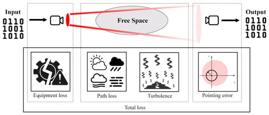
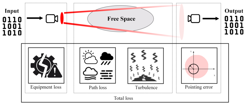
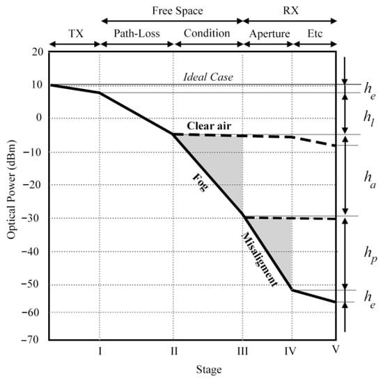
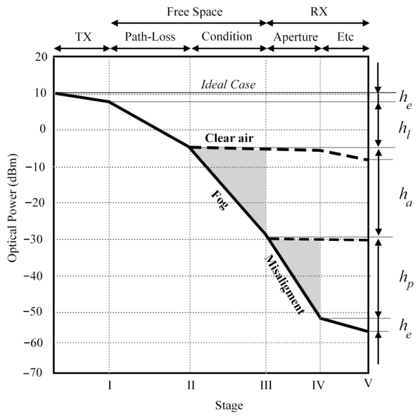
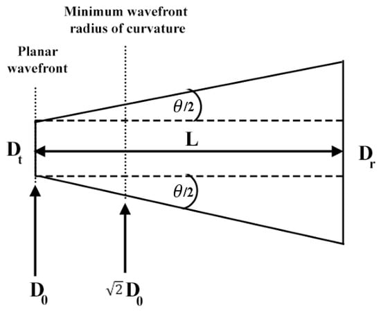
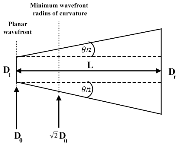
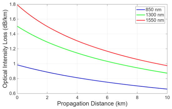
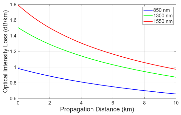
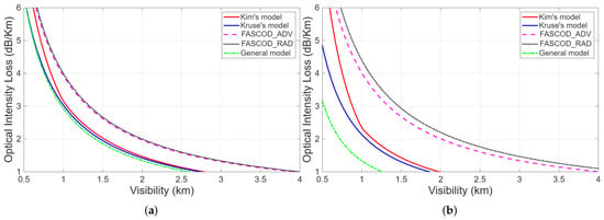
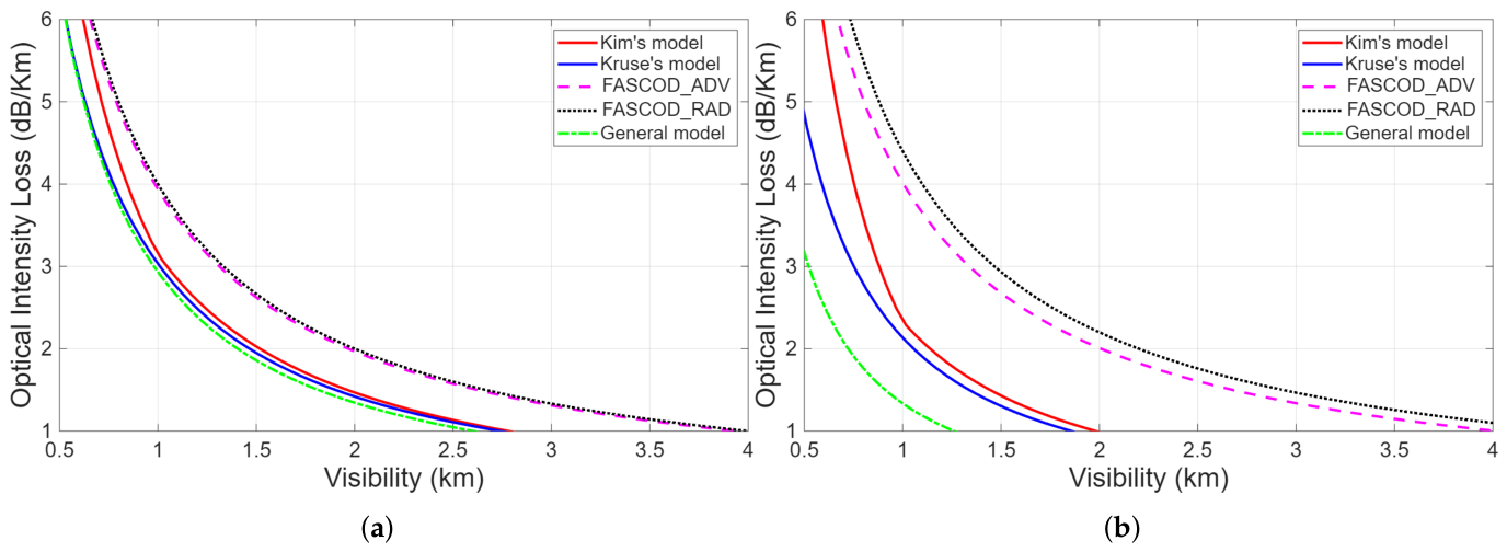
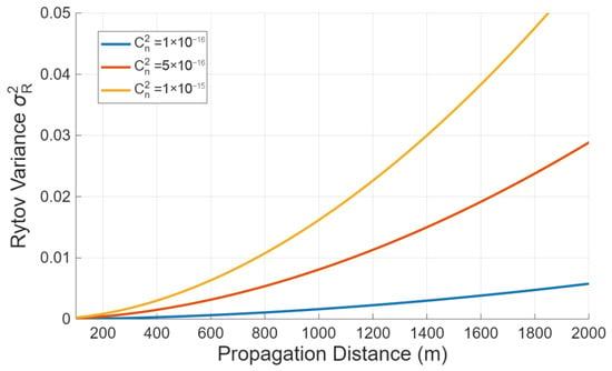
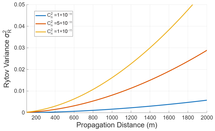
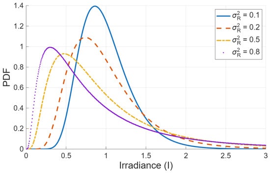
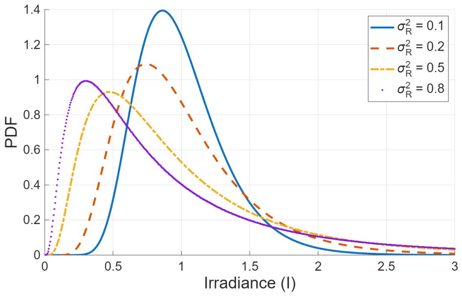
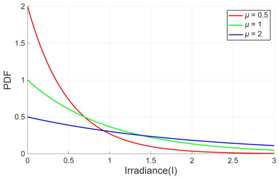
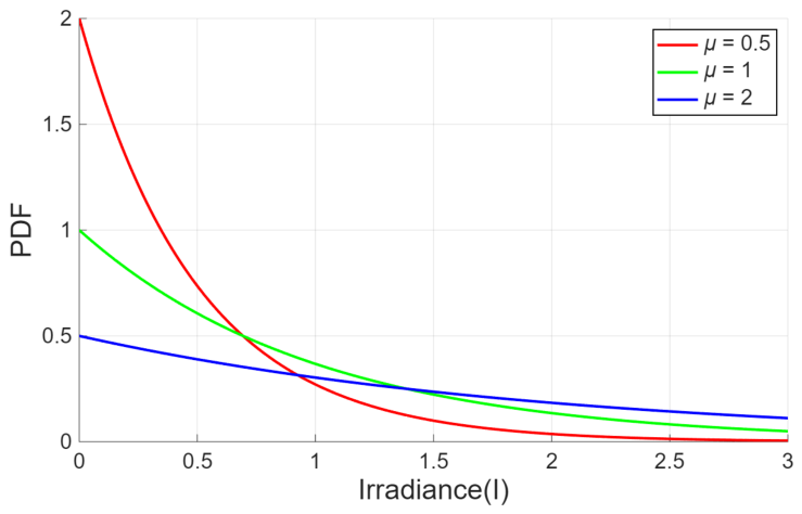
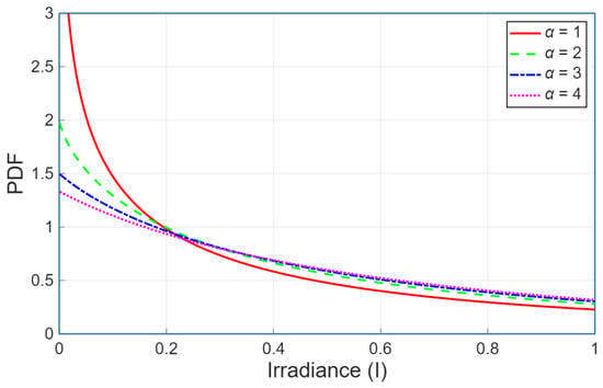
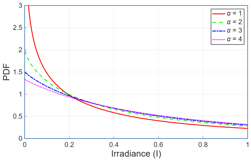
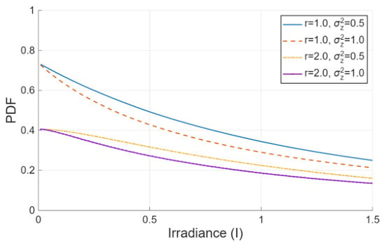
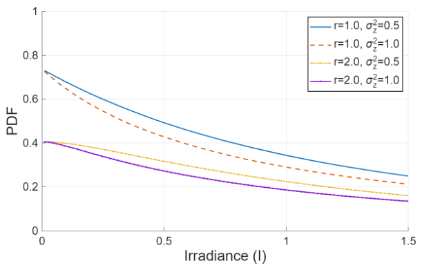
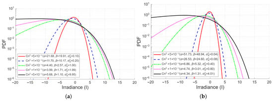
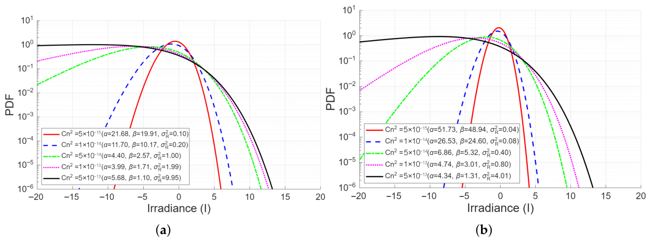
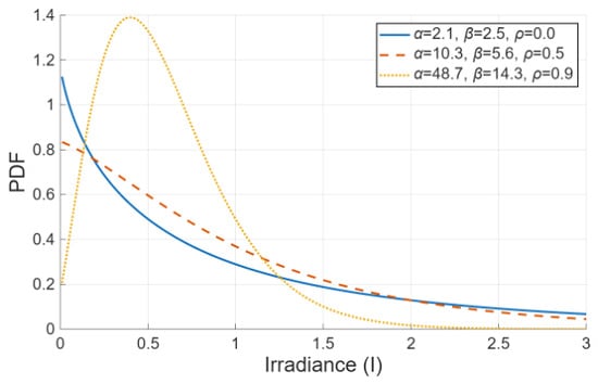
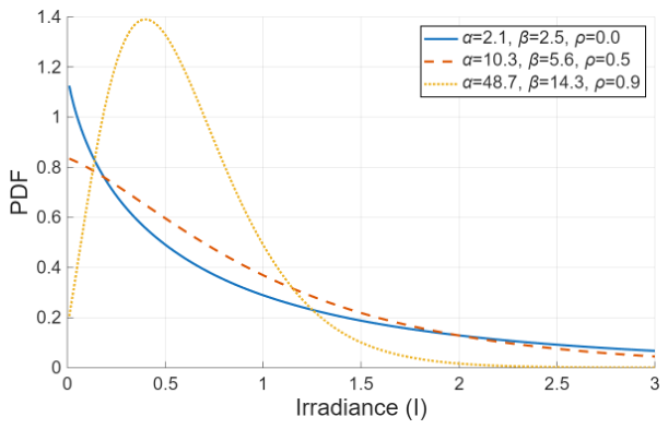
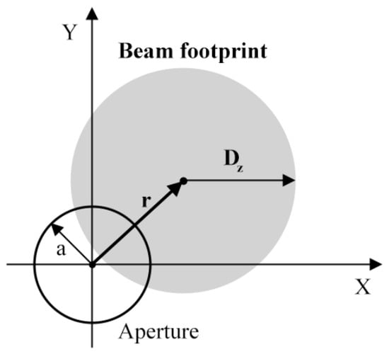
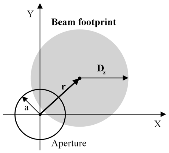
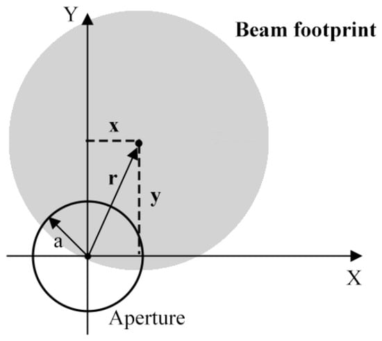
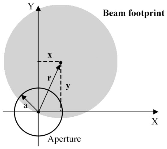
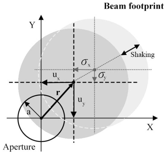
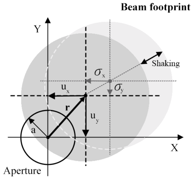
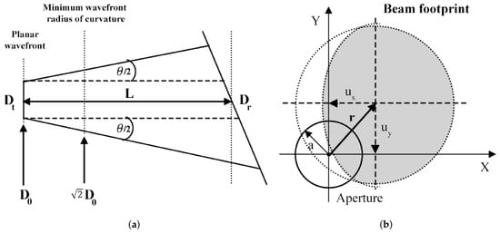
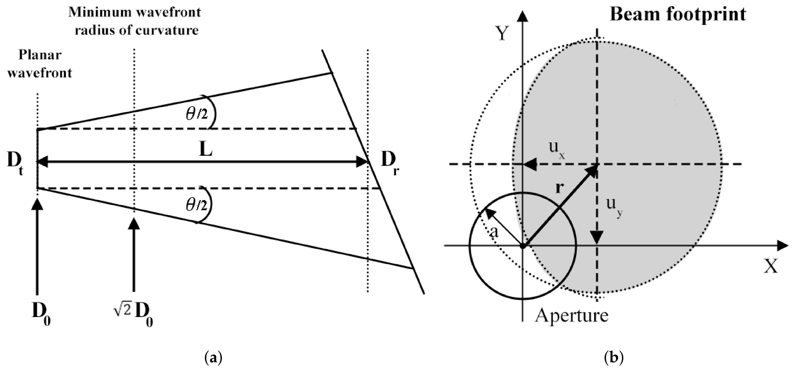
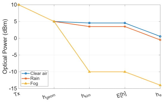
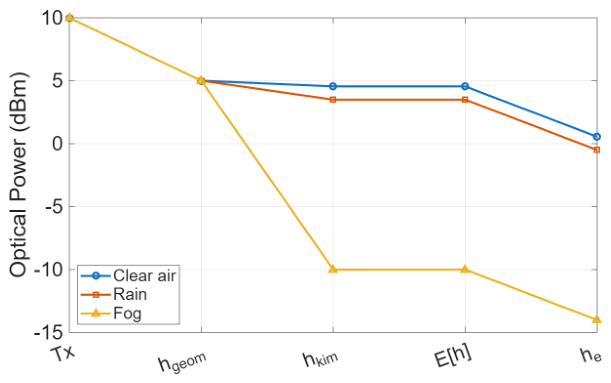
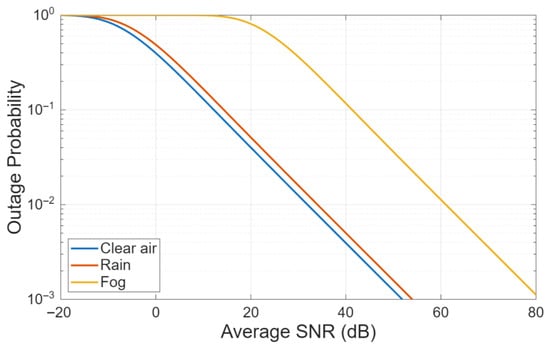
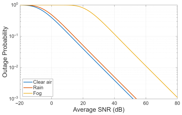
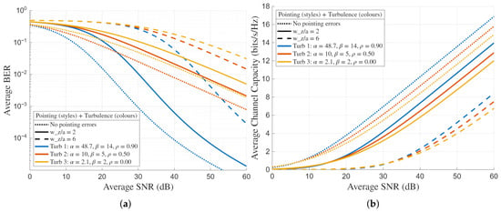
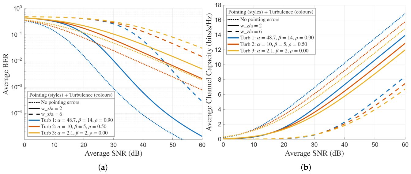
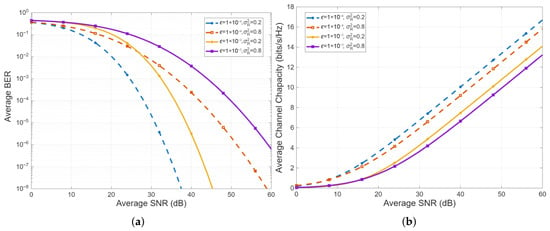
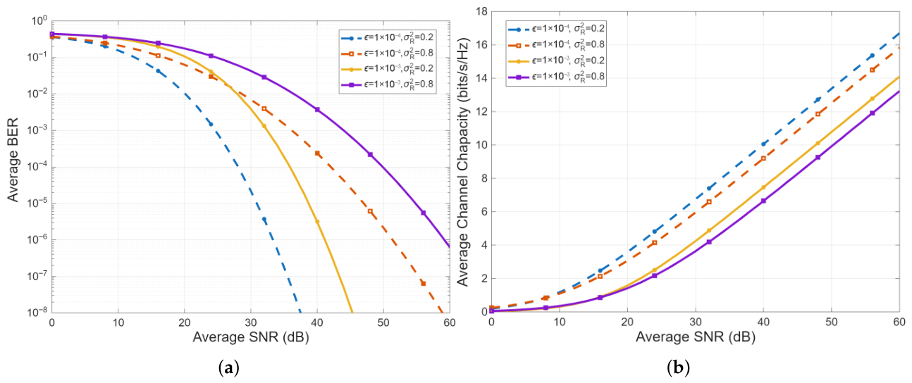

Disclaimer/Publisher’s Note: The statements, opinions and data contained in all publications are solely those of the individual author(s) and contributor(s) and not of MDPI and/or the editor(s). MDPI and/or the editor(s) disclaim responsibility for any injury to people or property resulting from any ideas, methods, instructions or products referred to in the content. |
© 2026 by the authors. Licensee MDPI, Basel, Switzerland. This article is an open access article distributed under the terms and conditions of the Creative Commons Attribution (CC BY) license.