


Abstract
Existing super-resolution evaluation systems for fluorescence microscopy images struggle to effectively detect potential artifacts in weak signal reconstruction. This study aims to establish a multi-dimensional evaluation framework that integrates frequency-domain evidence to verify the reliability of super-resolution techniques under low signal-to-noise ratio (SNR) conditions. All ground-truth (HR) images used in this study are experimentally acquired fluorescence microscopy data; the corresponding low-quality inputs are simulated from HR via controlled degradations (e.g., bicubic downsampling and frequency-truncation-based degradation) to enable paired quantitative evaluation. We designed a hierarchical comparative experiment to systematically evaluate the performance differences of CNN (SRCNN/FSRCNN), GAN (Real-ESRGAN), and Transformer (SwinIR) architectures on nucleus and whole-cell structure datasets. This study reveals a significant decoupling between “visual sharpness” and “signal fidelity”: while Real-ESRGAN can generate highly impactful high-frequency textures, its checkerboard effect in the spectrum and random residuals in the error map expose serious “illusion” risks, making it unsuitable for precise quantitative analysis. All ground-truth (HR) images used in this study are experimentally acquired fluorescence microscopy data; the corresponding low-quality inputs are simulated from HR via controlled degradations (e.g., bicubic downsampling and frequency-truncation-based degradation) to enable paired quantitative evaluation.
1. Introduction
In life sciences and biomedical research, fluorescence microscopy is widely used to observe subcellular structures such as the cell nucleus, cytoskeleton, and cell wall due to its molecular specificity and multi-channel imaging capabilities. However, microscopic imaging is inevitably constrained by the optical diffraction limit, exposure dose, acquisition speed, and phototoxicity. To reduce photobleaching and phototoxicity, experiments typically require reducing exposure time or excitation power, which directly leads to a decrease in the signal-to-noise ratio (SNR) and significantly weakens the visibility and resolvability of fine structures, especially in weak-signal fluorescence channels [1,2]. Therefore, improving the effective resolution of weak-signal channels without increasing the experimental burden while ensuring the credibility of structural recovery has become a critical research topic in computational enhancement and learning-based reconstruction [3,4].
The difficulties in weak-signal fluorescence channels are not simply manifested as “more blurry,” but rather a double loss at the information level: on the one hand, noise can overwhelm the high-frequency components corresponding to edges and textures; on the other hand, when high-frequency information is attenuated by the system transfer function, learning-based super-resolution may produce results that are “visually sharper but not necessarily more realistic.” For biological interpretation, this uncertainty directly affects the quantitative analysis of the cell nucleus boundary, weak textures, and fine structures, making researchers concerned about whether the recovered details are “reliable and verifiable” [5].
However, in weak signal imaging, relying solely on traditional metrics (such as PSNR and SSIM) to evaluate reconstruction quality has limitations. These pixel-based metrics tend to favor smooth reconstruction results and fail to capture the loss or spurious generation of high-frequency textures. Especially when the original signal is extremely weak, an ‘improvement’ in algorithm performance does not necessarily equate to a ‘credible’ result. This lack of evaluation dimensions makes it difficult for researchers to determine whether super-resolution details that are ‘visually clearer but of unknown origin’ conform to physical reality.
In recent years, deep learning has significantly advanced the development of denoising, deconvolution, and super-resolution in microscopic images. Unlike traditional reconstruction methods, learning-based methods learn a mapping from low-quality to high-quality images through large-scale paired data [4]. In the field of general image super-resolution, classic convolutional networks like SRCNN laid the foundation [6], while GAN-based methods emphasize perceptual quality and texture enhancement, with Real-ESRGAN being a representative framework [7,8]. More recently, Transformer architectures have excelled in capturing long-range dependencies, with SwinIR introducing the Swin Transformer into image restoration as a strong baseline [9]. These methods have been rapidly adapted to microscopic data tasks, providing feasible paths for reconstruction under complex degradation conditions [10].
However, improvement in algorithmic performance metrics does not always guarantee trustworthy results. While PSNR and SSIM excel at measuring pixel-domain errors, they struggle to answer critical questions in microscopy: Do the recovered details align with the true imaging mechanism? Are there spurious structures introduced by network priors? Especially under low-SNR conditions, models may “complete” textures through statistical priors. This makes evaluations solely based on PSNR/SSIM prone to potential misinterpretations [5].
From an optical and signal processing perspective, resolution is closely related to spatial frequency response. Therefore, the evaluation target should focus on whether “frequency-domain evidence supports structural recovery.” Introducing frequency-domain analysis helps determine which frequency components are reliably recovered and whether the minimum resolvable structure scale has been substantially improved. Related metrics have been continuously developed to robustly characterize the quality of complex microscopic data [11].
Meanwhile, deep learning is entering higher-risk microscopic reconstruction tasks, such as robust reconstruction of structured illumination microscopy (SIM). Recent work has demonstrated that super-resolution is possible under insufficient illumination contrast [12], while emphasizing uncertainty quantification to align with reproducibility requirements [13]. This indicates a necessary shift from single-pixel domain metrics to a framework combining pixel metrics with frequency-domain evidence to systematically support reliability assessment [14].
Based on this motivation, this study proposes an evaluation narrative of “from PSNR to frequency evidence” for low-SNR fluorescence channels. Under unified settings, we conduct a quantitative comparison of representative methods (SRCNN, FSRCNN, Real-ESRGAN, SwinIR) and analyze pixel metrics alongside frequency-domain evidence to improve the interpretability and reproducibility of weak signal reconstruction [15].
2. Materials and Methods
This paper presents a reliability assessment of super-resolution methods on multi-channel fluorescence microscopy images. All experiments focus on the reconstruction quality of low signal-to-noise ratio (SNR) channels, comparing various representative super-resolution methods under a unified data preprocessing pipeline, a unified method for generating low-quality input data, where low-quality inputs are simulated from experimentally acquired HR images via controlled degradations to form paired data for reproducible evaluation, and unified training and inference strategies. To avoid inflated test metrics due to the common similarity of neighboring samples in microscopy data, the training, validation, and test sets are divided by field of view or original acquisition unit, ensuring that adjacent frames or highly similar samples from the same field of view do not appear across different sets. For evaluation, this paper reports both pixel-domain metrics (PSNR, SSIM) and frequency-domain evidence correlation measures to characterize the overall error level and the recovery of spatial frequency information, thus further examining the reliability of fine structures and boundary continuity in low SNR channels beyond numerical metrics. The following sections describe the data and channel composition, channel extraction and quality control, simulated low-quality input generation (from experimental HR) and task setting, data partitioning strategy, training and inference configurations of the comparison methods, and evaluation metrics and statistical reporting methods.
2.1. Data and Channel Definition
This paper uses multi-channel fluorescence microscopy images to conduct super-resolution reliability assessment. To avoid semantic confusion between channels, this paper defines “channels” based on experimental labels or acquisition wavelengths, rather than using pseudocolor display colors as the naming basis. Each sample is represented as a multi-channel observation in the same field of view, where is the two-dimensional intensity image of the c channel. This paper focuses on “low signal-to-noise ratio target channels,” which correspond to different experimental semantics in different data domains: in the nuclear staining data domain, the target channel is the nuclear staining blue channel (denoted as Blue (DAPI, nucleus)); in the full-size cell structure data domain, the target channel is the structure-related blue acquisition channel (denoted as Blue (structural channel)). Although this channel is displayed with a blue pseudocolor, its structural representation shows continuous cellular structures rather than nuclear staining features; therefore, this paper does not equate it to DAPI. To maintain consistency throughout the paper, subsequent sections will refer to the two types of blue channels as “Blue (DAPI, nucleus)” and “Blue (structural),”, respectively, and the results will be reported separately for each data domain in the evaluation and statistics, avoiding conflating channels with different biological markers or different acquisition wavelengths as the same type of task at the semantic level.
The data in this paper is organized into two data domains. The first data domain is the nucleus-related staining data domain, which includes the White, Blue (DAPI, nucleus), and Red channels. This domain is used to evaluate the method’s ability to restore boundary continuity and detail stability under conditions where the nuclear structure is the primary target. The second data domain is the full-size cellular structure data domain, which includes the Green (FITC) and Blue (structural channel) channels. The Green (FITC) channel typically has a higher signal-to-noise ratio and more complete structural visibility, while the Blue (structural) channel is more susceptible to weak signals and background noise, forming a typical low signal-to-noise ratio reconstruction evaluation scenario. The channel configurations and basic specifications for both data domains are summarized in Table 1. All subsequent degradation generation, data partitioning, training and inference configurations, and evaluation metrics are based on the channel definitions in Table 1.
Table 1.
Dataset summary and channel properties.
2.2. Channel Extraction, Quality Control, and Intensity Normalization
To ensure that subsequent degradation generation, model training, and evaluation metric calculations are based on consistent data, this paper performs uniform channel extraction, quality control, and intensity normalization on multi-channel microscopic images before the data enters the learning process. Since raw microscopic data is typically stored in a multi-dimensional hyperstack format (including metadata such as channels, time, Z-axis, and spatial calibration), this paper prioritizes a general import method that can simultaneously parse pixels and acquisition metadata, exporting multi-channel data from the same field of view as single-channel intensity images while maintaining consistent spatial sampling. Specifically, Fiji is used as the data organization and visualization environment, and the Bio-Formats importer is used to read the raw files, preserving channel dimensions and basic spatial calibration information, thus avoiding channel order errors or loss of spatial scale caused by manual conversion [11,12]. During the export stage, each channel is saved as a separate single-channel grayscale image (prioritizing the original bit depth, usually 16-bit TIFF), and a fixed naming convention is used to encode sample identifiers and channel semantics, such as “sampleID__domain__channel.tif,” where the channel field strictly distinguishes between Blue (DAPI, nucleus) and Blue (structural channel) to avoid mixing channel semantics across data domains in subsequent experiments. For pseudocolor rendering required for paper presentation, LUTs are only applied during the visualization stage; all training and evaluation are performed based on the exported raw grayscale intensity values.
Quality control aims to remove anomalous samples that systematically interfere with training and evaluation, focusing on three common problems in microscopic imaging that significantly affect super-resolution results: defocusing or severe blurring, overexposure saturation, and significant field-of-view drift/streak artifacts. This paper employs consistent QC criteria for each data domain: First, we perform a quick screening of single-channel images after export. If an image exhibits large areas of saturation (e.g., a large number of pixels reaching the bit depth limit), completely unrecognizable defocus blur, or obvious non-biological streaks/occlusions, it is deemed an unqualified sample and removed from the training and testing sets. Second, a consistency check is performed on the multi-channel alignment, as cross-channel evaluation and frequency-domain evidence analysis assume that structures in the same field of view are spatially comparable. For multi-channel data acquired from the same field of view, the acquisition system generally ensures a common field of view between channels. However, if individual samples show significant channel misalignment or drift (e.g., visible shifts in boundary structures between channels), to avoid misinterpreting registration errors as super-resolution artifacts, this paper removes such samples without additional geometric registration processing, thus ensuring that the evaluation results primarily reflect the model’s capabilities rather than the influence of the registration algorithm. For more automated quality metrics, this paper uses frequency-domain-based image quality estimation as an auxiliary reference in supplementary experiments (e.g., FRC-type quality estimation), but the main process still relies on unified sample exclusion criteria to ensure data consistency and auditability [6].
The goal of intensity normalization is to eliminate intensity scale differences caused by different fields of view and acquisition conditions, while also preventing extreme bright spots or background biases from becoming dominant factors in model training. This paper uses the same normalization strategy for all channels: First, each image is cropped based on high and low percentiles to suppress the influence of outliers, and then linearly scaled to a fixed range. Let the original single-channel image be I. Select the intensity thresholds and corresponding to the low percentile and high percentile . The clipped and normalized image is
Clip (∙) denotes truncation to the [0, 1] range. This processing maps image intensities to uniform scale without introducing additional denoising or background removal algorithms, facilitating training and comparison of different models within the same dynamic range, while allowing the peak value L of PSNR to be consistently set to 1 in subsequent evaluations. To ensure traceability of the evaluation, this paper records the cropping thresholds (a, b) and channel identifiers for each image during the data preprocessing stage, enabling consistent inverse normalization if needed to return to the original scale for visualization or further analysis. For full-size data domains, if a stable camera bias causes an overall background elevation, this paper only allows passive handling through the aforementioned percentile cropping, without additional background subtraction or filtering, to avoid mistakenly weakening the true weak signal structures in different channels by treating them as background, thus maintaining that the evaluation object remains “the ability to recover structures under weak signal conditions”.
As shown in Figure 1, this study performed channel extraction, quality control, and intensity scale normalization on multi-channel fluorescence images before model training and evaluation, ensuring that subsequent experiments were conducted under consistent data representation and dynamic range. (a) A false-color composite image of the same field of view is provided to illustrate the spatial correspondence and semantic meaning of different channels; the false color is for visualization purposes only and is not used as model input. (b) Examples of channel-by-channel grayscale images derived from the same field of view are shown, including a reference channel with a high signal-to-noise ratio and the target blue channel. All subsequent models are trained and inferred based on this type of single-channel grayscale intensity image. (c) Typical examples of discarded samples during the quality control stage are shown, where out-of-focus frames with indistinguishable structures or samples with obvious acquisition anomalies are removed to avoid interference from invalid samples on training convergence and evaluation credibility. (d) The distribution changes of the target channel intensity before and after normalization are shown; normalization uses percentile clipping and linear mapping to [0, 1] to unify the dynamic range and ensure that different methods are comparable under the same intensity scale (the “mapped to [0, 1] before normalization” in the figure is only for visualizing and aligning the coordinate axes; the actual normalization rule is based on percentile clipping and scaling).
Figure 1.
Channel extraction, quality control, and intensity normalization for multi-channel fluorescence data.
2.3. Degradation Generation and Task Setting
This paper formulates the super-resolution learning of the target blue channel as a mapping problem from low-resolution observations to high-resolution structures. For any high-resolution image of the target channel, denoted as , the corresponding low-resolution input is constructed through a predefined degradation operator . The model learns a mapping such that the reconstructed high-resolution image approximates as closely as possible. This paper employs two types of degradation generation methods consistent with the implementation paths on different model families (SRCNN/FSRCNN, Real-ESRGAN, SwinIR): one is the classic bicubic interpolation downsampling (used in the ×4 experiments of SRCNN and FSRCNN), and the other is “high-frequency truncation simulation + bicubic downsampling” (used in the experiments of Real-ESRGAN and SwinIR), so as to more directly characterize the constraint of insufficient high-frequency information on reconstruction under weak signal conditions.
Under the bicubic downsampling setting, the low-resolution input is obtained by downsampling the high-resolution image, which can be written as
where represents the bicubic downsampling operator at a multiplier of s. In the experiments of SRCNN and FSRCNN, we set s = 4 and kept the input and output as single-channel grayscale intensity representations of the target blue channel, so that the network learning objective focuses on detail restoration and edge continuity reconstruction.
Under the setting of “high-frequency truncation simulation + bicubic downsampling”, this paper first suppresses the high-frequency components of high-resolution images in the frequency domain to simulate the situation of missing effective high-frequency information in weak signal imaging and then performs bicubic downsampling to obtain . This process can be written as
where and represent the two-dimensional Fourier transform and inverse Fourier transform, respectively; represents pointwise multiplication; and is the frequency-domain weighting function used to suppress energy in the high-frequency region while preserving the main structure in the low-frequency region. This mechanism is used in this paper to construct an input scenario that more closely resembles the “insufficient high-frequency information” of weak signal channels and serves as a unified degradation construction logic for the Real-ESRGAN and SwinIR experiments.
About data pairing, in this study, denotes experimentally acquired HR microscopy images. The corresponding low-quality inputs are simulated from using predefined and fully reproducible degradation operators , in order to construct paired data required for quantitative fidelity evaluation (e.g., PSNR/SSIM and frequency-evidence correlations). We note that physically acquired LR observations may involve additional microscope-specific effects (e.g., system PSF, Poisson–Gaussian noise, and non-uniform aberrations). Therefore, the conclusions in this paper are primarily established under the controlled paired setting; validation on physically acquired unpaired experimental LR is left as future work.
For any degradation setting, the basic form of the model input and output remains consistent: the input is the target blue channel’s , the output is the of the target blue channel, and the corresponding is used as the monitoring signal. In subsequent guided setups, the input can be expanded to a channel-by-channel concatenation representation of the “reference channel and target blue channel” , but the output and all evaluation metrics are still calculated only on the target blue channel to ensure that the task definition and comparison objects do not drift.
In addition to the two primary degradations used for model-family consistency, we further evaluate the stability of the proposed frequency-based diagnostics under additional plausible degradation variants (blur and Poisson–Gaussian noise) using the same experimental HR test images.
To operationalize these additional plausible degradation variants, we define two robustness-test operators based on blur and Poisson–Gaussian noise. Let denote the experimentally acquired high-resolution (HR) target image (normalized intensity), and sss be the downsampling factor (set to s = 4 to match the main experiments). The first variant introduces Poisson–Gaussian noise after bicubic downsampling:
where denotes bicubic downsampling by a factor of s. models a Poisson–Gaussian noise process, i.e.,
in which is an intensity-to-photon scaling parameter controlling the strength of the shot noise, and is the standard deviation of the additive Gaussian read noise (both defined in the normalized intensity domain). In this work, we use a fixed setting and for robustness testing.
The second variant further incorporates mild optical low-pass effects by applying Gaussian blur in the HR domain prior to bicubic downsampling, followed by the same Poisson–Gaussian noise model:
where denotes convolution with an isotropic Gaussian kernel of standard deviation (in HR pixels). We set to represent mild blur consistent with plausible microscope/defocus-induced low-pass behavior. Importantly, these parameters are introduced as fixed stress-test settings to evaluate the stability of the proposed frequency-based diagnostics under plausible degradation variations, rather than as an instrument-specific calibration of the imaging system noise model.
Table 2 summarizes the selection of degradation operators, scaling factor settings, and input/output formats for different data domains and model families in this paper, serving as a structured description of the task settings in this section.
Table 2.
Degradation settings and task definition used for different model families.
To complement the operator-level summary in Table 2, we provide visual examples of the HR inputs and the corresponding degraded observations used in this study. Figure 2 (nucleus domain) and Figure 3 (full-size structural domain) illustrate the primary degradation applied in each data domain—sLQ-A (bicubic downsampling) for the nucleus dataset and sLQ-B (high-frequency truncation followed by bicubic downsampling) for the full-size dataset—together with two additional plausible variants introduced for robustness evaluation. Specifically, sLQ-C adds Poisson–Gaussian (PG) noise on top of the primary degradation, and sLQ-D further includes a Gaussian blur prior to downsampling, followed by the same PG noise. For clarity and direct comparability, the same ROI is highlighted on the full images (yellow box) and shown as magnified crops in the right panels, allowing the reader to visually inspect how each degradation alters local structure and noise characteristics while keeping the underlying experimental HR content fixed.
Figure 2.
Degradation examples for the nucleus dataset (516 × 444).
Figure 3.
Degradation examples for the full-size dataset (1280 × 1280).
2.4. Data Splitting and Leakage Control
To ensure that subsequent experimental conclusions reflect only the differences between the model and the training strategy, and are not amplified by “approximate repetition” caused by adjacent frames, repeated sampling within the same field of view, or nearby slices, this paper explicitly models the hierarchical structure of the samples during the data organization stage and formulates splitting rules accordingly. Specifically, fluorescence microscopy data typically includes dimensions such as field of view (FOV), time series (t), and Z-stack (z). Within the same FOV, adjacent t or z samples often have highly similar structural morphology and background noise distribution. If the splitting is only based on “random partitioning by image file/patch,” nearby frames within the same FOV may be simultaneously assigned to both the training and test sets, resulting in highly similar content to the training samples during the testing phase. This leads to a systematic overestimation of the metrics and weakens the credible interpretability of the evaluation. Based on the above observations, the splitting strategy in this paper prioritizes isolation at a higher level, that is, first completing the partitioning of training, validation, and testing using “field of view/sequence” as the basic unit, and then generating corresponding HR/LR pairs and training samples within each subset.
At the implementation level, this paper first assigns a unique group identifier g to each image. This identifier is determined by its acquisition hierarchy information and is used to constrain the absence of shared nearest neighbor sources between different subsets. For full-size data domains, each original acquisition file or each FOV can be used as a group unit; for sequence data containing time or Z-stacks, all {t,z} under the same FOV are considered as the same group to avoid adjacent frames from crossing sets. Let the dataset be . The corresponding group identifier set is . The splitting process is performed at the level of , resulting in a set of non-overlapping groups , satisfied as
Accordingly, each subset is defined as follows:
After the split is completed, this paper applies the degradation operator defined in Section 2.3 to generate and supervision signal within each subset, thereby ensuring that the input and output construction process of training, validation, and testing is consistent and does not introduce data sharing across sets.
For model families trained using patches, this paper treats patch extraction as a secondary sampling process within a subset: training patches are extracted only from , validation patches are extracted from , and during the testing phase, inference and metrics are calculated only on using either a full image or a sliding window approach. This constraint avoids implicit leakage caused by different patches of the same full image appearing cross-referenced between training and testing. For settings involving full image training or full image inference, the group-level splitting principle is still followed to ensure that images from the same group are not reused across sets.
Furthermore, to reduce the random fluctuations caused by data splitting, this paper maintains consistency in coverage across subsets under key acquisition conditions during splitting, including the intensity range of the target channel, the morphological diversity of samples, and the background noise level. This consistency is not achieved through additional filtering or resampling, but rather through statistical checks after group-level partitioning to ensure that both the training and test sets contain representative distributions of weak signal samples. Thus, this paper establishes a data splitting and leakage control process that matches the microscopic data structure, providing a stable data foundation for subsequent comparisons of different models and loss designs.
For each data domain, we split images into training/validation/testing sets using an approximately 7:2:1 ratio at the acquisition-unit (field-of-view) level to prevent near-duplicate leakage across sets. For the nucleus dataset (N = 185), this corresponds to 130/37/18 images for training/validation/testing, respectively; for the full-size dataset (N = 742), this corresponds to 520/148/74 images. All methods compared within the same data domain use exactly the same split lists.
2.5. Comparison of Model and Implementation Settings
This paper selects four representative super-resolution models as comparison objects, covering four main technical routes, “classic convolutional baseline-lightweight convolution acceleration-adversarial perception enhancement—Transformer structural modeling”, so as to facilitate comparative analysis of the reconstruction performance of low signal-to-noise ratio blue channel from the aspects of structural modeling ability and reconstruction style. Specifically, they include SRCNN, FSRCNN, Real-ESRGAN and SwinIR. SRCNN, as an early end-to-end convolutional super-resolution model, uses shallow convolutional networks to directly learn the mapping from low resolution to high resolution and is one of the classic pixel domain baselines [5]. FSRCNN introduces a more compact structure and deconvolution upsampling design on the SRCNN idea to improve inference efficiency and maintain good reconstruction quality, and it is suitable as a lightweight convolutional comparison. Real-ESRGAN is aimed at real degradation scenes and uses generative adversarial training to improve visual quality and texture perception effects, representing the “perception-first” reconstruction route [6]. SwinIR, based on the windowing attention mechanism of Swin Transformer, demonstrates stronger long-range dependency modeling and structural recovery capabilities in image restoration tasks, and it can serve as a strong baseline for Transformer-type models [7].
Regarding input and output definitions, this paper adopts a unified “target blue channel super-resolution” setting for all models: In single-channel tasks, the model input is the target blue channel’s , and the output is the same channel’s . For the Real-ESRGAN and SwinIR experiments, the low-resolution input adopts the degradation construction of “high-frequency truncation simulation + bicubic downsampling” as described in Section 2.3. For the SRCNN and FSRCNN experiments, the low-resolution input adopts the ×4 bicubic downsampling construction [6,7]. During the training and inference stages, each model outputs the reconstruction results of the target blue channel and uses them for subsequent pixel-domain and frequency-domain index calculations; the differences in model structure are only reflected in the feature extraction and reconstruction strategies, without changing the task definition and output channels.
To minimize confounding effects from unequal training budgets across architectures, all methods within the same data domain are trained using identical train/validation/test split lists (7:2:1) and the same epoch schedule, with the total number of training epochs fixed across models. Model selection is performed on the validation subset, and all quantitative results are computed on the held-out test subset only. Therefore, the comparisons reported in this work reflect differences in reconstruction behavior under a controlled training budget rather than differences in training duration.
2.6. Evaluation Metrics and Frequency-Domain Evidence
About units and normalization, unless otherwise stated, all microscopy images are intensity-normalized to prior to training and evaluation; therefore, pixel intensities and error-map values are reported in arbitrary units (a.u.) under this normalization. Spatial axes in all image displays, line profiles, and ROI crops are in pixels (px). PSNR is reported in decibels (dB) with after normalization, while SSIM is unitless. For frequency-domain visualizations and radial spectra, the horizontal axis represents the discrete spatial-frequency index (dimensionless) derived from the 2D FFT grid (from DC toward the Nyquist limit), and spectral magnitude/power is shown in a.u. (log-scaled where applicable).
The evaluation object in this paper is always limited to the reconstruction result of the target blue channel and compared with the corresponding reference image in the same intensity coordinate system. To ensure the numerical comparability between different methods, all images are uniformly scaled to [0, 1] before calculating the index. For cases with boundary interpolation or padding, the evaluation is only performed within a consistent effective area to avoid edge artifacts having a dominant influence on the index.
Pixel domain evaluation uses PSNR and SSIM. First, the mean squared error is defined:
where H,W represents the image size. Since the intensity range in this paper is unified to [0, 1], the PSNR is calculated based on the peak value of L = 1.
SSIM is used to measure structural similarity and supplements it with reflections of brightness and contrast consistency. For a reference image patch x and a reconstructed image patch y within a local window, SSIM is defined as
Among them, x and y represent the reference image and the reconstructed image, respectively; and represent the mean of the image; and represent the variance of the image; is the covariance; and are stability constants used to avoid zero denominator. The value range of SSIM is [0, 1], where 1 indicates complete structural consistency; higher than 0.8 means that the original structural features are better preserved.
Relying solely on PSNR/SSIM may be insufficient to characterize the reconstruction reliability of low signal-to-noise ratio fluorescence channels. On the one hand, smoothing and noise reduction may improve PSNR/SSIM but simultaneously weaken the mid-to-high frequency information corresponding to true edges. On the other hand, some enhancement methods may introduce sharper appearance textures, but these high-frequency components may not be consistent with the reference image. To supplement the explanation of this type of “relationship between pixel-domain numerical improvement and structural reliability,” this paper introduces frequency-domain evidence as an auxiliary evaluation dimension, directly observing the information recovery of the reconstruction results at the spatial frequency level.
Frequency-domain evidence is based on two-dimensional Fourier transform. Frequency-domain representations are calculated for both the reference image and the reconstructed image:
and take its amplitude spectrum:
This paper employs two methods to report frequency-domain evidence. The first is amplitude spectrum visualization: and are logarithmically compressed and displayed to visually compare whether the energy distribution of different methods in the mid-to-high frequency region is consistent with the reference, and whether there is abnormal high-frequency enhancement or excessive attenuation. The second is radial average spectrum curves: the amplitude spectrum is statistically analyzed according to the frequency radius to obtain one-dimensional spectrum curves ) and , used to compare whether the attenuation trend and bandwidth extension of different methods in the mid-to-high frequency band are closer to the reference image. To avoid the influence of overall amplitude scale differences on the comparison, the spectrum curves can be uniformly normalized when displayed (e.g., normalized according to low-frequency energy or total energy), so that the focus of the comparison is on the relative changes in the frequency band shape and the high-frequency part.
In the results analysis, this paper interprets pixel-domain metrics and frequency-domain evidence together: when a method simultaneously improves PSNR/SSIM and is closer to in the mid-to-high frequency range, and no anomalous frequency components corresponding to non-reference structures appear in the amplitude spectrum, it can be interpreted as more reliable structure recovery; conversely, if the improvement in pixel-domain metrics is accompanied by a significant deviation in spectral shape or abnormal expansion of high-frequency energy, it needs to be cautiously interpreted as appearance enhancement or metric bias risk. Regarding the comparative description of the “minimum resolvable structure scale” mentioned in the paper, this paper uses the effective extension of the frequency-domain spectral curve at the high-frequency end as a reference, converting it to a spatial scale to reflect the relative changes in the resolvability of fine structures by different methods. This scale is used for comparison and interpretation between methods rather than for recalibrating the physical limits of the imaging system.
2.7. External Dataset Evaluation for Generalization Beyond Synthetic Degradation Pairs
To assess the generalization of the proposed frequency-domain evaluation beyond the synthetic degradation pairs used in this study, we additionally conducted an external benchmark test on the ER (endoplasmic reticulum) subset of the publicly available BioSR dataset [16]. BioSR-ER provides paired low-resolution (LR) and ground-truth (GT) fluorescence microscopy images released on figshare, enabling quantitative evaluation on an independent experimental data distribution. All external experiments were performed in a strict inference-only setting: the pretrained models were directly applied to BioSR-ER without any retraining, fine-tuning, or parameter search on the external data.
We followed the LR/GT pairing defined by the dataset. For each pair, the LR image was used as the model input to generate the super-resolved output (SR), which was then compared against the corresponding GT image. BioSR-ER is provided at a native ×2 scale (e.g., LR 128 × 128 and GT 256 × 256), whereas the models evaluated in this paper are configured with a fixed ×4 up-scaling factor. To ensure a consistent spatial resolution for comparison, we applied a deterministic scale-alignment step to the LR input: the native LR image was downsampled by an additional factor of 2 using bicubic interpolation (128 × 128 → 64 × 64) and then fed into the ×4 model to produce a 256 × 256 SR output, matching the GT dimensions. This scale-alignment operation was applied to LR inputs only, identically for all models, and solely to reconcile the mismatch between the external dataset’s native scale and the fixed ×4 inference setting.
For spatial-domain evaluation, PSNR and SSIM were computed between SR and GT and averaged over the external test set. For frequency-domain evaluation, we computed (i) the two-dimensional log-power spectrum using a 2D FFT followed by spectrum centering (fftshift), and (ii) the radial average power spectrum (RAPS) by radially averaging the spectral power over concentric frequency rings. The normalized spatial frequency was defined as the spectral radius divided by min (H, W)/2 to ensure comparable frequency axes across images. In addition to reporting quantitative metrics, we visualize representative GT/SR pairs together with their corresponding spectra and RAPS curves to characterize model-dependent deviations in reconstructed frequency content.
Finally, we note that BioSR-ER provides paired LR/GT data for quantitative benchmarking on an independent experimental distribution. Fully unpaired (LR-only) experimental scenarios would require no-reference evaluation or additional data acquisition, and are discussed as future work.
3. Results
This section reports experimental results for two data domains. Section 3.1 introduces the image patch-level Blue (DAPI, cell nucleus) benchmark, demonstrating the performance of local structure reconstruction and its frequency-domain characteristics; Section 3.2 introduces the full-field Blue (structure channel) benchmark, demonstrating the structural continuity and frequency-domain energy distribution over a large field of view. Due to the different field-of-view scales and sampling characteristics of the two data domains, this section does not directly compare the values from different data domains but instead uses a consistent evaluation dimension within each data domain to present the results. Finally, to generalize the conclusions and increase the applicability of the samples, the BioSR-ER dataset is introduced for evaluating the model.
Unless otherwise stated, all images used for quantitative evaluation are intensity normalized to [0, 1]; therefore, pixel intensity and error are expressed in arbitrary units (a.u.). In patch-level results, spatial coordinates are expressed in pixels (px); when a scale bar is displayed in the figure, its unit is micrometers (µm), and the scale bar length is obtained based on the spatial calibration of the original CZI metadata. PSNR is reported in decibels (dB) (MAX = 1 after normalization), and SSIM is dimensionless. In the frequency-domain results, the frequency axis represents the spatial frequency index of the discrete FFT grid (pointing from DC to Nyquist, with a dimensionless dimension), and the spectral amplitude/power is displayed on a logarithmic scale (a.u., labeled as log magnitude in the figure).
3.1. Patch-Level Comparison of Convolutional Baselines: SRCNN vs. FSRCNN
This subsection compares SRCNN and FSRCNN on the low-SNR Blue (nucleus) patch-level benchmark. To make architectural differences easier to interpret, we present the two models side-by-side under the same evaluation dimensions: (i) spatial reconstruction appearance and pixel-domain metrics, (ii) pixel-wise absolute error morphology, (iii) 1D intensity profile consistency, and (iv) frequency-domain evidence via 2D log-spectrum and RAPS.
3.1.1. Spatial Reconstruction and Quantitative Metrics
Table 3 summarizes the average quantitative metrics of each model on the entire validation set, providing a quantitative basis for comparing the performance of different models. It compares the reconstruction results of SRCNN and FSRCNN side-by-side with the ground truth for easy visual observation and also shows the visual reconstruction image of FSRCNN on the validation set (Figure 4). Visually, compared to bicubic interpolation input, both SRCNN and FSRCNN can suppress some background noise, but their reconstruction results still exhibit a noticeable smoothness, with limited ability to recover fine-grained textures in low signal-to-noise ratio regions. Furthermore, the FSRCNN output image shows similar characteristics to SRCNN in terms of smoothness and edge sharpness.
Table 3.
Quantitative comparison of average PSNR and SSIM on the validation set ().
Figure 4.
Visual comparison of SRCNN and FSRCNN (patch-level Blue channel). All images are intensity-normalized to (a.u.); spatial coordinates are in pixels (px). PSNR is reported in dB with , and SSIM is unitless.
In terms of quantitative metrics, on the current test samples, SRCNN achieved a peak signal-to-noise ratio (PSNR) of 23.96 dB and a structural similarity index (SSIM) of 0.3753. The lower SSIM value indicates its limitations in preserving the original image structural information. According to the average quantization data in Table 3, FSRCNN achieved a mean PSNR of 26.25 dB on the validation set, an improvement of 0.36 dB compared to SRCNN’s 25.89 dB and significantly better than the baseline level of 24.44 dB for traditional bicubic interpolation. Notably, unlike the performance trade-offs typically seen in accelerated models, FSRCNN also achieved an improvement in structural similarity (SSIM), reaching 0.5856, higher than SRCNN’s 0.5762.
3.1.2. Error Distribution Analysis (Pixel-Wise Absolute Error)
To analyze the spatial distribution of reconstruction error, we computed the pixel-wise absolute difference, , between the reconstructed image and the ground-truth image, and we visualized it as an error heatmap in Figure 5 (left: SRCNN; right: FSRCNN). In both heatmaps, the background region shows a widespread distribution of cyan values, with absolute errors mainly around 0.04–0.06, while the region of interest (ROI), particularly around the cell nucleus boundary and locally high-intensity textures, contains concentrated red/yellow patches with higher absolute errors (e.g., >0.12). The error values are reported in a.u. under [0, 1] intensity normalization.
Figure 5.
Pixel-wise absolute error maps of SRCNN and FSRCNN. Errors concentrate at structural edges (red/yellow regions), indicating a failure to recover high-frequency boundaries. The error map visualizes the absolute error . is reported in a.u. under the intensity normalization, and spatial coordinates are in pixels (px).
3.1.3. Structural Intensity Consistency (1D Profile)
To evaluate two models’ ability to preserve fluorescence signal intensity, we performed a one-dimensional intensity profile analysis on row y = 200 of the image, as shown in Figure 6.
Figure 6.
Intensity profile comparison at y = 200. The profile is extracted along the horizontal line y = 200; the x-axis is pixel coordinate (px) and the plotted intensities are in a.u. under normalization. Curves: Ground Truth (black), SRCNN (red), FSRCNN (red dashed or another distinguishable style).
Figure 6 presents the one-dimensional intensity profile analysis performed at row y = 200 of the image, comparing the intensity distributions of the Ground Truth (GT, black solid line), SRCNN (red solid line), and FSRCNN (red dashed line) reconstructions. The GT intensity profile exhibits dramatic high-frequency fluctuations, reflecting the noise characteristics and subtle textures of the original low-SNR fluorescence signal. The SRCNN reconstruction follows the overall intensity trend of the GT but fails to reproduce its high-frequency oscillations, instead appearing as a smooth approximation; notably, at the signal peak near x = 370, SRCNN’s predicted intensity is significantly attenuated relative to the GT peak. FSRCNN shows a similar smooth fluctuation pattern in non-peak regions (e.g., x = 400–800), also failing to capture the GT’s high-frequency details, though its predicted intensity at the x = 370 peak (≈180 gray levels) is higher than that of SRCNN (≈150 gray levels), both remaining below the GT’s actual peak of ≈200 gray levels.
3.1.4. Frequency-Domain Evidence (2D Spectrum and RAPS)
Pixel-domain metrics alone cannot distinguish “over-smoothing” from “artifact-like high-frequency injection.” We therefore compare frequency-domain evidence using (i) 2D log-spectrum visualization and (ii) radial average power spectrum (RAPS).
For the 2D frequency representation, Figure 7 places SRCNN, FSRCNN, and Ground Truth spectra in one consolidated figure. SRCNN exhibits a rapid decay toward high frequencies (dark corners), consistent with low-pass behavior and spatial over-smoothing. FSRCNN introduces more structured spectral energy around the center; however, the spectrum also shows periodic grid-like patterns, consistent with deconvolution-related checkerboard artifacts. Importantly, the presence of additional high-frequency components does not necessarily indicate faithful recovery of true structural frequencies.
Figure 7.
Consolidated 2D log-frequency spectra (patch-level). Panels: (a) SRCNN spectrum, (b) FSRCNN spectrum, (c) Ground Truth spectrum. Frequency axes correspond to discrete spatial-frequency indices of the 2D FFT grid (dimensionless, DC → Nyquist), and the color indicates log spectral magnitude in a.u.
For quantitative frequency comparison, Figure 8 overlays RAPS curves for SRCNN, FSRCNN, and Ground Truth. In the low-frequency range, both models track the Ground Truth relatively closely. As frequency increases (your current narrative uses the “>20” threshold), both SRCNN and FSRCNN fall below the Ground Truth, indicating insufficient recovery of the high-frequency tail where fine biological structures reside. FSRCNN may show local deviations consistent with artifact-related energy, but the overall high-frequency deficit relative to the Ground Truth remains.
Figure 8.
RAPS curve comparison (patch-level). The x-axis denotes the radial spatial-frequency index of the discrete FFT grid (dimensionless bin from DC toward Nyquist), and the y-axis shows log power in a.u. Curves: Ground Truth (black), SRCNN (red dashed), FSRCNN (red solid).
3.2. Full-Field Comparison of Advanced Models: Real-ESRGAN vs. SwinIR (Blue, Full-Size)
This section presents a comparative analysis of the reconstruction results of Real-ESRGAN and SwinIR on the full-scale Blue (structural channel) data domain. To facilitate observation under the same evaluation dimension, this section reports the results from four aspects in turn: (i) full-scale and ROI magnification visualization and quantitative indicators, (ii) pixel-level absolute error distribution, (iii) one-dimensional intensity profile alignment, and (iv) frequency-domain evidence (2D log-spectrum and RAPS).
3.2.1. Spatial Reconstruction and Quantitative Metrics (Full + ROI Zoom)
Table 4 (quantitative comparison on the full-size dataset, ×4) summarizes the average quantitative metrics for Bicubic and Real-ESRGAN on the full-size dataset, providing an overall numerical benchmark within this data domain. The table shows that Bicubic has an average PSNR of 26.15 dB and an average SSIM of 0.4038 under the ×4 condition; Real-ESRGAN has an average PSNR of 26.00 dB and an average SSIM of 0.3700 under the ×4 condition. Therefore, Table 4 provides a comparison of the PSNR/SSIM values of the two methods in the full-size dataset under the same evaluation criteria.
Table 4.
Quantitative comparison of average PSNR and SSIM on the full-size Blue dataset (×4).
Figure 9 (visual comparison of Real-ESRGAN and SwinIR on the full-size dataset with ROI zoom) shows a visual comparison of the full-size reconstructions of Real-ESRGAN, Ground Truth, and SwinIR, with ROIs at the same location marked in yellow boxes on the three full-size images. The second row further shows the magnified results of the corresponding ROIs, used for detailed comparison of the same local area. The example image also labels the PSNR/SSIM of a single sample in the panel title: Real-ESRGAN (Full) is 25.98 dB/0.3869, and SwinIR (Full) is 26.85 dB/0.4289. In terms of image interpretation, the first row is mainly used to observe the structural continuity and consistency of brightness and darkness distribution across the entire dataset; the second row of magnified ROIs is used to observe differences in texture undulations, boundary transitions, and fine-grained structural presentation within local areas. Since the three images use the same ROI coordinates, the differences in the ROI rows directly correspond to differences in the reconstructed appearance of the same spatial content.
Figure 9.
Visual comparison of Real-ESRGAN and SwinIR on the full-size Blue dataset (full field with ROI zoom). Top row: full-field reconstructions with the same ROI marked by the yellow box. Bottom row: enlarged views of the ROI. All images are intensity-normalized to [0, 1] (a.u.). PSNR is reported in dB with MAX = 1, and SSIM is unitless.
3.2.2. Error Distribution Analysis (Pixel-Wise Absolute Error)
Figure 10 (pixel-wise absolute error maps |SR − GT|) shows the pixel-wise absolute error heatmaps (|SR − GT|) of Real-ESRGAN and SwinIR relative to the Ground Truth. Both error maps use the same color scale to represent the error magnitude range. When interpreting the maps, the error magnitude can be directly understood through color: large areas of dark blue/cyan correspond to lower errors, gradually increasing towards green, yellow, and then orange–red, corresponding to higher errors. Both error maps cover the entire field of view, thus allowing simultaneous observation of (i) the error “noise” pattern and coverage in the background area, (ii) whether more concentrated high-error patches appear in structurally distinct areas (e.g., areas with strong boundaries/contrast changes), and (iii) whether high-error areas exhibit localized clustering or scattered spatial distribution.
Figure 10.
Pixel-wise absolute error maps of Real-ESRGAN and SwinIR on the full-size dataset, visualizing . Errors are reported in a.u. under [0, 1] normalization. Color indicates absolute error magnitude.
As seen in Figure 10, the Real-ESRGAN error map is predominantly blue–cyan across the entire image, with scattered higher error points/patches visible. The SwinIR error map is also predominantly blue–cyan, but it also includes a color bar on the right, facilitating the mapping of local color variations to the error value range. Both maps share the characteristic that the error is not concentrated in a single small area, but rather appears as a combination of “overall background distribution + local higher error points/patches,” allowing the reader to simultaneously obtain global and local error information on the same image.
3.2.3. Structural Intensity Consistency (1D Profile)
Figure 11 (Intensity profile overlay at y = 200 px) shows a comparison of one-dimensional intensity profiles overlaid along the same horizontal line (y = 200 px). In the figure, the black curve represents the Ground Truth, the red dashed line represents Real-ESRGAN, and the red solid line represents SwinIR; the horizontal axis represents pixel coordinates X (px), and the vertical axis represents normalized intensity (a.u.). When interpreting the figure, focus on three aspects: first, whether the three curves maintain a similar upward/downward trend globally; second, whether the red line aligns with the black line at the peak positions near major peaks and troughs; and third, whether the local fluctuations of the red line match or exhibit a smoother trend relative to the black line in sections with dense undulations in the curves.
Figure 11.
Intensity profile comparison at y = 200 px (full-size). The profile is extracted along a horizontal line. X-axis: pixel coordinate (px). Y-axis: normalized intensity (a.u.) under [0, 1] normalization. Curves: Ground Truth (black), Real-ESRGAN (red dashed), SwinIR (red solid).
As can be directly seen from the superposition effect in Figure 11, the Real-ESRGAN and SwinIR curves generally follow the main trend of the GT curve and show a relatively obvious change in the same direction as GT in several major peak and valley sections. In the local area with more rapid fluctuations, the difference in appearance between the red line and the black line, which is “closer or smoother”, is also easier to observe, because the three curves are superimposed in the same coordinate system, and any local deviation will be reflected by a visible gap.
3.2.4. Frequency-Domain Evidence (2D Spectrum and RAPS)
Figure 12 (Consolidated 2D log-frequency spectra) places the 2D spectra (log magnitude) of Real-ESRGAN, SwinIR, and Ground Truth side-by-side in the same image. Each spectrum panel is accompanied by a corresponding color bar to indicate the range of log spectrum magnitudes. When interpreting the image, first observe the brightness and expansion pattern of the central region (near DC), then check the uniformity of the energy distribution outward from the center (in the direction of higher spatial frequencies), and finally look for regular, repeating texture patterns (such as dot matrix patterns, square/ring-shaped “boundaries,”, etc.), as these patterns will appear as more regular bright spots or regular structures in the 2D spectrum. In terms of visual presentation in Figure 12, the Real-ESRGAN spectrum panel shows a more obvious distribution of regular bright spots (appearing as dot-like repeating structures); the SwinIR spectrum panel shows a larger-scale symmetrical structure outside the central region (presenting a more obvious sense of shape boundaries); the Ground Truth spectrum panel is dominated by central brightness, presenting a relatively continuous background energy distribution outward.
Figure 12.
Consolidated 2D log-frequency spectra (full-size). Panels: (a) Real-ESRGAN spectrum, (b) SwinIR spectrum, (c) Ground Truth spectrum. Frequency axes correspond to discrete spatial-frequency indices of the 2D FFT grid (dimensionless, from DC toward Nyquist). Color indicates log spectral magnitude in a.u.
Figure 13 (RAPS curve overlay) shows the overlay curve of the radial average power spectrum (RAPS), used to compress 2D spectral information into a 1D curve to observe the overall trend of radial frequency (bins) variation. In the figure, black represents GT, red dashed line represents Real-ESRGAN, and red solid line represents SwinIR; the horizontal axis is the radial frequency bins (from DC to Nyquist), and the vertical axis is the log magnitude (dB). When reading the graph, you can view it in the order of low frequency, mid frequency, and high frequency: in the low-frequency segment, mainly observe whether the three curves are close to each other; as the frequency increases, observe how the spacing between the red and black lines changes; at the high-frequency end, focus on whether the red line still maintains a close trend with the black line or shows a more obvious separation. As shown in Figure 13, the two method curves are closer to the GT curve at the low-frequency end. Subsequently, as the radial frequency increases, the difference between the red and black lines gradually becomes more visible. At higher frequencies, Real-ESRGAN (red dashed line) and SwinIR (red solid line) maintain a lower curve position relative to GT (black line), and there is also a visible difference between the two red lines, making the curve spacing in the high-frequency range one of the most intuitive comparison information in the figure.
Figure 13.
RAPS curve comparison (full-size). X-axis denotes the radial spatial-frequency index (bins) of the discrete FFT grid (dimensionless, from DC toward Nyquist). Y-axis shows log magnitude (dB). Curves: Ground Truth (black), Real-ESRGAN (red dashed), SwinIR (red solid).
3.3. Validation Results on External Public Datasets (BioSR-ER)
To supplement the result presentation under external data distribution, this study further conducted external testing on the ER (endoplasmic reticulum) subset of the publicly available microscopic super-resolution dataset BioSR [16]. This dataset is publicly released fluorescence microscopy image data, providing paired low-resolution (LR) and high-resolution (GT) images, which can be used to reproduce experiments and perform quantitative comparisons on independent data sources. This section’s external testing used 100 LR/GT paired samples from the ER subset, maintaining the original pairing relationships of the dataset; all models underwent only forward inference and evaluation, without any form of retraining, fine-tuning, or parameter search, to ensure that the results reflect the direct output performance of the model on the external data distribution.
Regarding size alignment, the pairing relationship provided by the BioSR-ER subset is native ×2 (LR is 128 × 128, GT is 256 × 256), while the magnification of the deep learning model compared in this paper is fixed at ×4. To achieve spatial size consistency with the ground truth (GT), external testing performed deterministic scale alignment on the LR input: the native LR image was further downsampled by a factor of 2 (128 × 128 → 64 × 64) through bicubic interpolation and then input into a ×4 model to generate a 256 × 256 SR output, thus achieving strict spatial alignment with the corresponding GT. Based on this aligned SR and GT, this study statistically analyzed the PSNR and SSIM in the spatial domain and calculated the mean and standard deviation for 100 samples for quantitative summary comparison.
Table 5 summarizes the quantitative results (mean ± std, N = 100) on the external test set. The bicubic interpolation baseline yielded a PSNR of 20.28 ± 2.34 dB and an SSIM of 0.6762 ± 0.0962 under this external test setting. The PSNR for FSRCNN was 14.01 ± 2.37 dB and the SSIM was 0.2945 ± 0.0986; for Real-ESRGAN, it was 18.10 ± 2.57 dB and the SSIM was 0.6177 ± 0.1014; and for SwinIR-KAIR, it was 15.62 ± 2.39 dB and the SSIM was 0.4657 ± 0.0579. In addition to quantitative summarization, this study also generated frequency-domain visualization outputs consistent with the main experiment for external test samples, including 2D log-power spectrum and RAPS curves, to provide a unified presentation of the frequency-domain performance of external data at the results level.
Table 5.
Quantitative results on the external BioSR-ER dataset (N = 100).
Figure 14 presents a visualization comparison of representative examples (im57) from the external dataset. This figure displays color-coded comparisons of SR and its corresponding GT according to model category, with PSNR and SSIM labeled for each example. It also provides the corresponding RAPS curves and a two-dimensional log-power spectrum visualization of GT/SR to maintain consistency with the presentation of the main experimental results. These figures collectively constitute the results of this study on publicly available external BioSR-ER data.
Figure 14.
Visualization comparison of representative examples (im57) from the BioSR-ER dataset.
4. Discussion
4.1. Decoupling of Perceptual Quality and Signal Fidelity in Generative Reconstruction
A significant finding of this study is that in low signal-to-noise ratio microscopy, perceived sharpness does not necessarily translate into pixel-level signal fidelity, a point fully demonstrated in the experimental results of Real-ESRGAN. Although the images generated by this model on the full-size dataset (Figure 9) exhibit extremely high contrast and clear cytoskeleton texture, their PSNR (25.98 dB) and SSIM (0.3869) are anomalously lower than the benchmark bicubic interpolation method. To elucidate the physical mechanism of this “perception-distortion” paradox, it is necessary to delve into the spatial distribution of pixel-level errors and the local consistency of signal intensity. The error heatmap of Real-ESRGAN (Figure 10) reveals an atypical error pattern: rather than structural edge deviations, it is more like cyan random noise diffused across the entire field of view. This distribution characteristic suggests that generative adversarial networks (GANs), when attempting to recover high-frequency information lost due to photon noise, tend to synthesize texture details that conform to the statistical laws of biological tissue but are spatially random. This randomness prevents the generated structure from achieving pixel-level alignment with the Ground Truth, significantly increasing the L1 error.
Intensity profile analysis further quantifies this signal offset. In Figure 11, while the intensity curve (red line) of Real-ESRGAN morphologically simulates the high-frequency oscillations of real fluorescence signals, giving the image a “textured” visual appearance, there is a significant amplitude mismatch between its absolute intensity values and the Ground Truth at key signal peaks and troughs (such as the x = 370 region). This oscillation is essentially a discriminator-driven “illusionary” texture, rather than a true reproduction of the original photon distribution. Therefore, while Real-ESRGAN offers visual advantages in qualitative visualization, the uncontrollable randomness it introduces may pose a potential risk of systematic bias to quantitative analyses that rely on precise grayscale values (such as fluorescence intensity measurement).
4.2. Structural Advantages of Non-Local Attention Mechanisms in Noise Suppression
Unlike convolutional neural networks (such as SRCNN) which tend to oversmooth due to limited local receptive fields, SwinIR, based on the Transformer architecture, demonstrates superior structure preservation in weak signal recovery tasks. SwinIR achieves the highest quantitative metrics (PSNR 26.87 dB/SSIM 0.4205) on a full-size dataset. This performance advantage can be directly attributed to its windowed multi-head self-attention (W-MSA) mechanism’s effective modeling of long-range dependencies. A comparison of error heatmaps clearly illustrates the impact of this architectural difference: unlike the high error bands generated at cell nucleus edges in SRCNN, SwinIR’s error map (Figure 10) exhibits a highly uniform dark cyan background with almost no structural edge residuals. This indicates that the model successfully utilizes non-local self-similarity within the image, repairing subtle details by referencing similar features outside the neighborhood, thus achieving effective separation and suppression of background thermal noise without blurring structural edges.
The intensity profile (Figure 11) provides more intuitive evidence for the “denoising” properties of SwinIR. The SwinIR prediction curve (red line) not only maintains a very high degree of fit with the Ground Truth in its overall trend but also exhibits a slightly smoother characteristic in local details. In the context of biological imaging, this slight smoothing is actually a correction for photon shot noise in the imaging system, rather than a loss of effective signal. The model distinguishes between “biological structures” and “random noise” through an attention mechanism, eliminating unstructured high-frequency perturbations while preserving the integrity of the main signal peak. This extreme pursuit of signal fidelity makes SwinIR a more reliable quantitative analysis tool than generative models.
4.3. Frequency-Domain Analysis as a Diagnostic Tool for Architectural Inductive Bias
In stark contrast, the SwinIR spectrogram (Figure 12) displays a unique cross-shaped asterism and symmetrical square halos. This is the result of the Swin Transformer’s operation of dividing the image into fixed-size windows for attention calculation, generating harmonic oscillations in the form of a Sinc function in the frequency domain. Although this is also an artificially introduced spectral feature, analysis of the RAPS curve (Figure 13) shows that the energy of SwinIR in the high-frequency range (frequency > 25) remains slightly lower than that of the Ground Truth. This does not imply a loss of high-frequency information but rather a frequency-domain response consistent with its spatial denoising characteristics—the model conservatively suppresses high-frequency components containing significant noise, recovering only biological signals with structural confidence. Therefore, strictly differentiating between “generative artifacts” (e.g., grid patterns in GANs) and “reconstruction fingerprints” (e.g., Sinc patterns in Transformers) in the frequency domain provides a practical gateway for reliability auditing. We suggest that frequency spectrum screening should serve as a standard “lie detector” before quantitative analysis: if a reconstructed image exhibits high-intensity geometric periodicities in the spectrum that are absent in the raw data, it should be flagged as “high risk” for morphological measurement tasks.
4.4. External Dataset Interpretation: Cross-Distribution Frequency Evidence (BioSR-ER)
The external BioSR-ER evaluation provides a stringent stress test for the central claim of this study: in weak-signal fluorescence microscopy, visually convincing reconstructions can deviate from the underlying signal statistics, and such deviations are more faithfully exposed in the frequency domain than by spatial-domain fidelity scores alone. When models trained and assessed under controlled degradations are confronted with an independent experimental distribution, the most informative outcome is not whether a method “wins” a single scalar metric but whether the frequency response of the reconstruction remains physically plausible and consistent with the Ground Truth spectrum.
A key observation from the BioSR-ER examples is that different architectures exhibit distinct frequency-response behaviors that align with their inductive biases. For convolutional reconstruction (e.g., FSRCNN), the spectrum and RAPS profiles typically reflect a conservative low-pass tendency: the reconstructed energy concentrates near low frequencies while mid-to-high frequency components decay rapidly. In the spatial domain this manifests as suppressed fine structures and reduced micro-texture contrast, but in the frequency domain it appears unambiguously as a systematic deficit in the mid-to-high frequency band relative to Ground Truth. This “missing-frequency” signature is important because it is not merely an aesthetic property; it indicates that the reconstruction behaves like a smoothing operator under cross-distribution uncertainty, prioritizing stability over detail recovery.
In contrast, generative reconstruction (e.g., Real-ESRGAN) can produce visually sharper boundaries and higher apparent texture richness, yet its frequency-domain evidence often reveals a different type of deviation: rather than simply restoring broadband high-frequency energy, the reconstruction may introduce structured spectral patterns that are weak or absent in the Ground Truth. In the 2D log-power spectrum, this can appear as directional streaks, cross-like asterisms, or periodic energy concentrations, which are consistent with the model’s tendency to synthesize plausible textures driven by learned priors rather than to reproduce the exact photon-limited signal realization. The practical implication is that a visually “enhanced” image can have a frequency composition that is statistically plausible but not necessarily signal-faithful at the pixel level—precisely the perceptual–fidelity decoupling emphasized in Section 4.1, now observed on an independent experimental dataset.
Transformer-based reconstruction (SwinIR-KAIR) exhibits yet another characteristic profile. While attention mechanisms can preserve global structural coherence and suppress unstructured noise, the frequency domain can still expose architecture-specific fingerprints associated with windowed self-attention and patch-wise processing, such as anisotropic spectral responses or subtle grid-aligned harmonics. Importantly, these signatures are not inherently “good” or “bad”; rather, they provide diagnostic cues indicating how the model redistributes energy across frequencies when faced with a distribution shift. In other words, the external dataset does not merely provide another benchmark; it demonstrates that the frequency-domain analysis proposed in this paper remains interpretable and discriminative across data sources, enabling reliability auditing that goes beyond visual inspection and beyond a single scalar metric.
Taken together, the BioSR-ER results strengthen the methodological contribution of this work: frequency-domain descriptors (2D log-power spectrum and RAPS) serve as a practical bridge between qualitative appearance and quantitative trustworthiness. They make it possible to separate two failure modes that are otherwise easily conflated in microscopy super-resolution—(i) under-reconstruction characterized by systematic high-frequency deficit and (ii) over-generation characterized by structured spectral anomalies—thereby supporting a more actionable interpretation of reconstruction reliability under cross-distribution testing.
4.5. Limitations and Future Perspectives
While the BioSR-ER experiment indicates that the proposed frequency-domain descriptors remain diagnostic under an independent data source, several limitations must be acknowledged to properly scope the conclusions of this study. First, the main paired evaluation protocol is constructed by applying controlled degradations to experimentally acquired HR images. Such degradations may not fully reflect the compound, system-dependent characteristics of real microscopy formation processes, including non-uniform wavefront aberrations, spatially varying point spread functions, and mixed noise statistics (e.g., Poisson–Gaussian behavior) that can differ across instruments and acquisition settings. The external BioSR-ER evaluation partially mitigates this concern by providing an independent experimental distribution; however, it still relies on paired supervision and a deterministic scale-alignment procedure and therefore does not fully represent genuinely unpaired, LR-only experimental scenarios where reference GT is absent.
Second, the current analysis is performed on static cellular structures. The temporal stability of the compared models in live-cell imaging remains unexplored, where motion blur, photobleaching, and rapid intensity fluctuations may introduce additional failure modes and distinct frequency-domain signatures. Third, this study prioritizes reconstruction quality and reliability auditing over computational efficiency. We did not systematically benchmark inference latency, throughput, or memory footprint—factors that are particularly relevant for high-throughput screening and may be non-negligible for computationally intensive architectures such as Transformer-based models. Finally, although the present work emphasizes the decoupling between perceptual sharpness and signal fidelity, translating frequency-domain evidence into actionable decision thresholds for specific downstream quantitative tasks (e.g., intensity-based measurements versus morphology-only visualization) warrants further task-dependent calibration.
To address these limitations, future research will focus on advancing both the evaluation framework and model interpretability. We plan to develop and release an open-source Frequency-Domain Evaluation Toolkit that automates spectral anomaly detection and fidelity screening, lowering the barrier for non-expert users to audit super-resolution outputs prior to quantitative analysis. In parallel, we will explore frequency-aware training objectives to better balance texture generation and structural fidelity under realistic noise conditions, and we will investigate uncertainty quantification mechanisms that predict pixel-level confidence maps alongside reconstructions. Such confidence-aware outputs would establish a clearer trust boundary, enabling practitioners to differentiate reliable biological recovery from algorithmic speculation in precision imaging workflows.
5. Conclusions
This study addresses the reliability issues of super-resolution reconstruction in low signal-to-noise ratio fluorescence microscopy. A multi-dimensional evaluation system encompassing spatial domain metrics, error distribution characteristics, and frequency-domain response features was established, systematically revealing the performance boundaries and inductive biases of different deep learning architectures in weak signal recovery tasks. Through comparative studies of convolutional neural networks (SRCNN/FSRCNN), generative adversarial networks (Real-ESRGAN), and the Transformer architecture (SwinIR), we confirmed a significant decoupling between “visual sharpness” and “signal fidelity” in the controlled paired evaluation setting constructed from experimentally acquired HR microscopy images. The results show that while generative models, such as Real-ESRGAN, can reconstruct visually striking high-frequency textures, the random distribution of pixel-level errors and the typical checkerboard artifacts in the frequency domain reveal that they are essentially texture synthesis based on statistical priors, rather than a precise restoration of the original biological signal. This reconstruction strategy, accompanied by the risk of “hallucination,” is unsuitable as a basis for rigorous quantitative analysis.
In contrast, the Transformer-based SwinIR model demonstrates structural robustness, which is more crucial in scientific imaging. Thanks to the effective modeling of long-range dependencies by the multi-head self-attention mechanism of the window, SwinIR successfully preserved weak subcellular structures while suppressing imaging thermal noise, achieving the highest PSNR/SSIM ratio and the most uniform error distribution on the full-size dataset. Although it employs a relatively conservative denoising strategy in the ultra-high frequency energy response, this “quality over quantity” characteristic ensures the reliability of the output results at the photon metrology level, making it an ideal choice for downstream analysis tasks such as fluorescence intensity quantification and structural segmentation. Furthermore, while traditional convolutional networks are efficient inference, they are limited by local receptive fields and struggle to overcome the bottleneck of excessive smoothing when processing low signal-to-noise ratio data, failing to meet the demands of high-precision imaging.
In summary, this study not only provides biologists with clear criteria for model selection but also advocates an evaluation paradigm that shifts from single numerical indicators to multi-dimensional frequency-domain evidence. We propose that in the process of AI-enabled microscopic imaging, relying solely on PSNR or visual observation, is insufficient to establish trust; we recommend that two-dimensional spectral analysis and radial average power spectrum be incorporated as a routine reliability check to flag potential frequency-domain artifacts, especially when pixel-domain metrics or visual inspection alone are insufficient. The establishment of this paradigm will help clarify the boundaries between “enhancement” and “generation” in computational imaging technology and promote the transformation of super-resolution technology from a simple visual optimization tool to a truly reliable and repeatable precision measurement instrument in life science research.
Author Contributions
For this work, H.H. took charge of methodology development, software design and implementation, method validation, formal analysis of experimental data, research direction investigation, data curation, preparation of the manuscript’s original draft, visualization of results, as well as review and editing of the manuscript. H.A. was responsible for the conceptualization of the study, provision of relevant resources, supervision of the overall research process, and project administration. All authors have read and agreed to the published version of the manuscript.
Funding
This research received no external funding.
Data Availability Statement
The microscopy dataset used in this study was accessed through the University of Glasgow data infrastructure and is subject to institutional data governance and access restrictions. Therefore, the full dataset cannot be made publicly available by the authors. To support reproducibility, the authors can provide (i) preprocessing and training scripts, (ii) the trained model weights, and (iii) a limited subset of anonymized sample pairs for benchmarking upon reasonable request, subject to institutional approval.
Acknowledgments
The authors would like to express sincere gratitude to the teaching and research team of the University of Glasgow for their academic guidance during the research process. Thanks are also extended to the technical support staff who provided assistance in the experimental process.
Conflicts of Interest
The authors declare no conflicts of interest.
Abbreviations
The following abbreviations are used in this manuscript:
| Adam | Adaptive Moment Estimation |
| CNN | Convolutional Neural Network |
| DAPI | 4′,6-diamidino-2-phenylindole |
| FFT | Fast Fourier Transform |
| FITC | Fluorescein isothiocyanate |
| GT | Ground Truth |
| HR | High Resolution |
| LR | Low Resolution |
| MSE | Mean Squared Error |
| PSNR | Peak Signal-to-Noise Ratio |
| Q/K/V | Query/Key/Value |
| ROI | Region of Interest |
| RSTB | Residual Swin Transformer Block |
| SNR | Signal-to-Noise Ratio |
| SR | Super-Resolution |
| SSIM | Structural Similarity Index Measure |
References
- Liu, S.; Hoess, P.; Ries, J. Super-resolution microscopy for structural cell biology. Annu. Rev. Biophys. 2022, 51, 301–326. [Google Scholar] [CrossRef] [Scilit] [PubMed]
- Adhikari, M.; Houhou, R.; Hniopek, J.; Bocklitz, T. Review of fluorescence lifetime imaging microscopy (FLIM) data analysis using machine learning. J. Exp. Theor. Anal. 2023, 1, 44–63. [Google Scholar] [CrossRef] [Scilit]
- Yang, T.; Luo, Y.; Ji, W.; Yang, G. Advancing biological super-resolution microscopy through deep learning: A brief review. Biophys. Rep. 2021, 7, 253. [Google Scholar] [CrossRef] [Scilit] [PubMed]
- Qiao, C.; Li, D.; Guo, Y.; Liu, C.; Jiang, T.; Dai, Q.; Li, D. Evaluation and development of deep neural networks for image super-resolution in optical microscopy. Nat. Methods 2021, 18, 194–202. [Google Scholar] [CrossRef] [Scilit] [PubMed]
- Dong, C.; Loy, C.C.; He, K.; Tang, X. Image super-resolution using deep convolutional networks. IEEE Trans. Pattern Anal. Mach. Intell. 2015, 38, 295–307. [Google Scholar] [CrossRef] [Scilit] [PubMed]
- Wang, X.; Xie, L.; Dong, C.; Shan, Y. Real-esrgan: Training real-world blind super-resolution with pure synthetic data. In Proceedings of the IEEE/CVF International Conference on Computer Vision, Montreal, BC, Canada, 11–17 October 2021; pp. 1905–1914. [Google Scholar]
- Liang, J.; Cao, J.; Sun, G.; Zhang, K.; Van Gool, L.; Timofte, R. Swinir: Image restoration using swin transformer. In Proceedings of the IEEE/CVF International Conference on Computer Vision, Montreal, BC, Canada, 11–17 October 2021; pp. 1833–1844. [Google Scholar]
- Wang, X.; Sun, L.; Chehri, A.; Song, Y. A review of GAN-based super-resolution reconstruction for optical remote sensing images. Remote Sens. 2023, 15, 5062. [Google Scholar] [CrossRef] [Scilit]
- Wang, X.; Yi, J.; Guo, J.; Song, Y.; Lyu, J.; Xu, J.; Yan, W.; Zhao, J.; Cai, Q.; Min, H. A review of image super-resolution approaches based on deep learning and applications in remote sensing. Remote Sens. 2022, 14, 5423. [Google Scholar] [CrossRef] [Scilit]
- Preusser, F.; Dos Santos, N.; Contzen, J.; Stachelscheid, H.; Costa, É.T.; Mergenthaler, P.; Preibisch, S. FRC-QE: A robust and comparable 3D microscopy image quality metric for cleared organoids. Bioinformatics 2021, 37, 3088–3090. [Google Scholar] [CrossRef] [Scilit] [PubMed]
- Chen, Y.; Liu, Q.; Zhang, J.; Ye, Z.; Ye, H.; Zhu, Y.; Kuang, C.; Chen, Y.; Liu, W. Deep learning enables contrast-robust super-resolution reconstruction in structured illumination microscopy. Opt. Express 2024, 32, 3316–3328. [Google Scholar] [CrossRef] [PubMed]
- Liu, T.; Liu, J.; Li, D.; Tan, S. Bayesian deep-learning structured illumination microscopy enables reliable super-resolution imaging with uncertainty quantification. Nat. Commun. 2025, 16, 5027. [Google Scholar] [CrossRef] [Scilit] [PubMed]
- Yan, B.; Ma, C.; Tan, W.; Sun, Y.; Fu, H. No-Reference Hallucination Assessment for AI-Reconstructed Fluorescence Microscopy Image. 2025. Available online: https://sciety.org/articles/activity/10.21203/rs.3.rs-7026761/v1?utm_source=sciety_labs_article_page (accessed on 23 December 2025).
- Schindelin, J.; Arganda-Carreras, I.; Frise, E.; Kaynig, V.; Longair, M.; Pietzsch, T.; Preibisch, S.; Rueden, C.; Saalfeld, S.; Schmid, B.; et al. Fiji: An open-source platform for biological-image analysis. Nat. Methods 2012, 9, 676–682. [Google Scholar] [CrossRef] [Scilit] [PubMed]
- Chen, C.; Wang, Y.; Zhang, N.; Zhang, Y.; Zhao, Z. A review of hyperspectral image super-resolution based on deep learning. Remote Sens. 2023, 15, 2853. [Google Scholar] [CrossRef] [Scilit]
- Qiao, C.; Li, D. BioSR: A Biological Image Dataset for Super-Resolution Microscopy. Figshare. Dataset. 2020. Available online: https://figshare.com/articles/dataset/BioSR/13264793/9 (accessed on 23 December 2025).
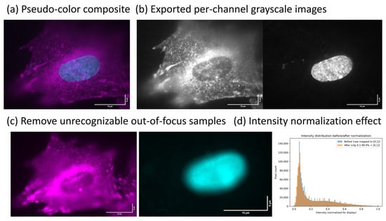
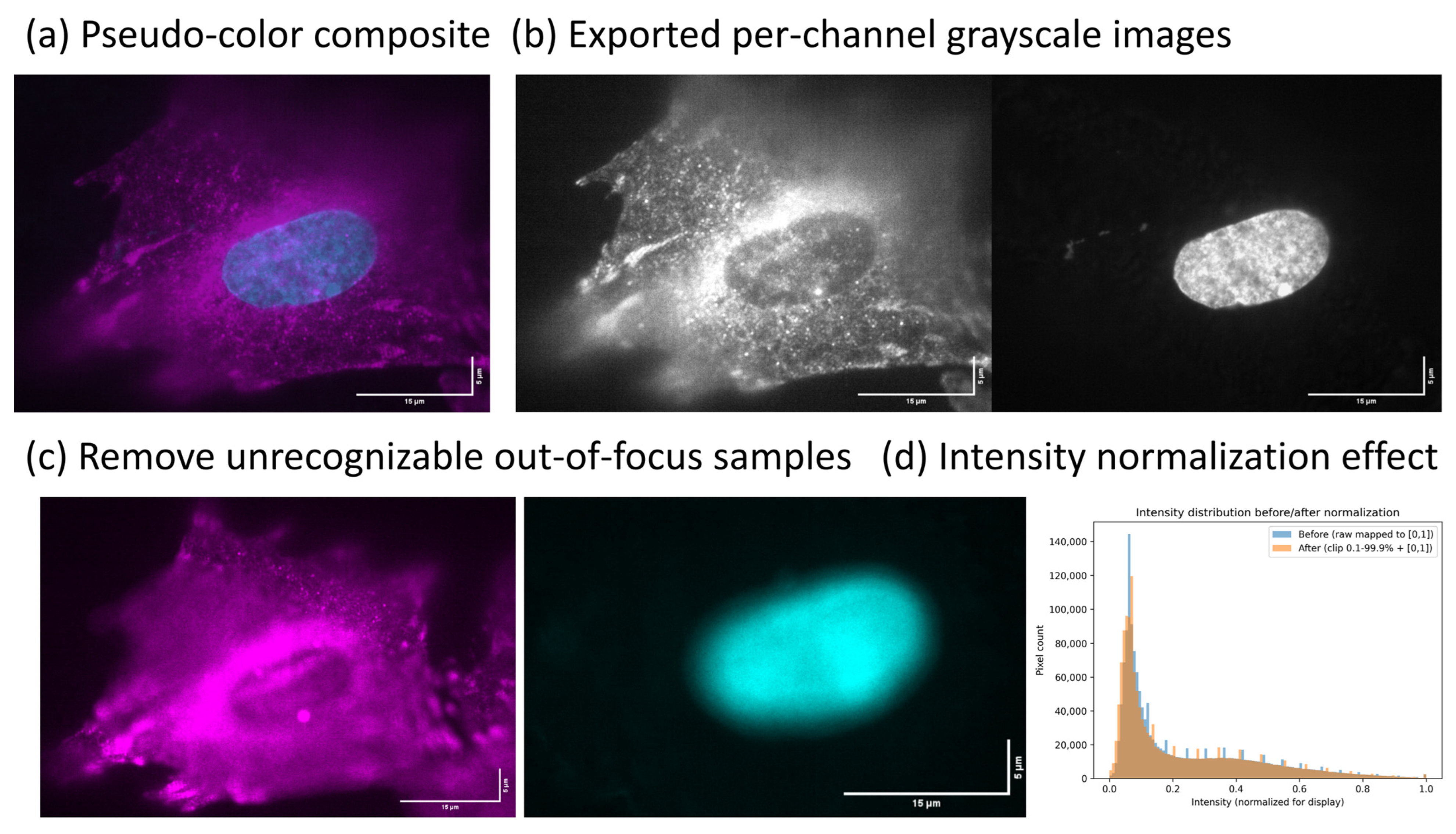
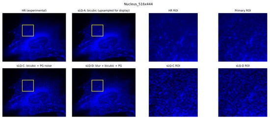
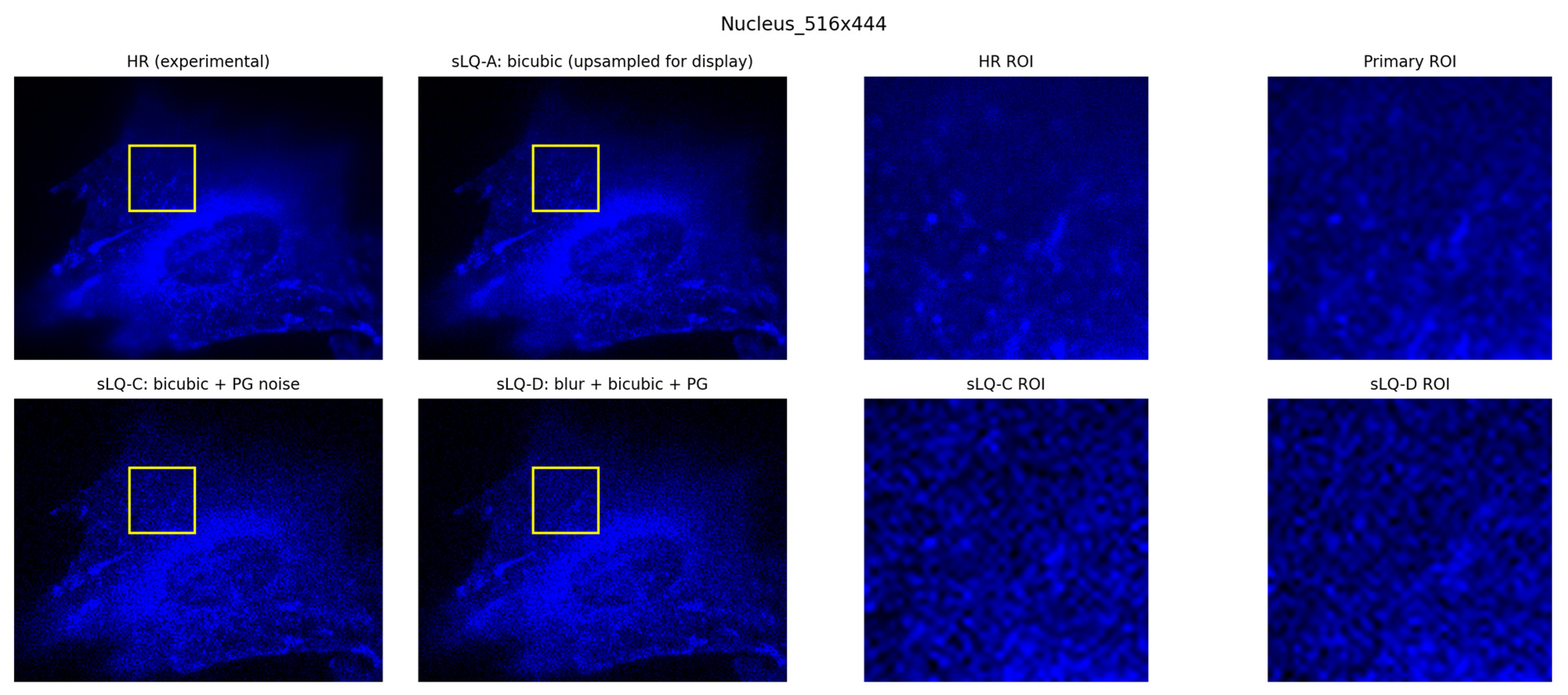
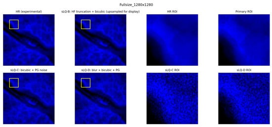
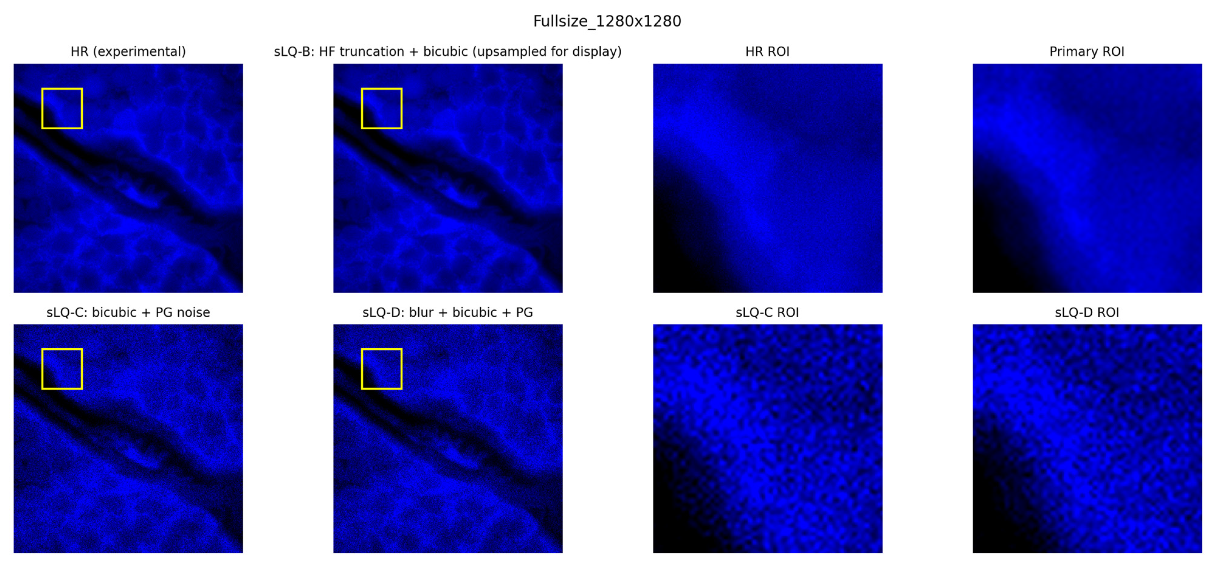
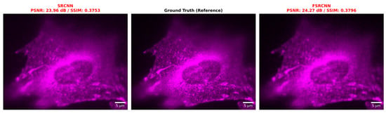
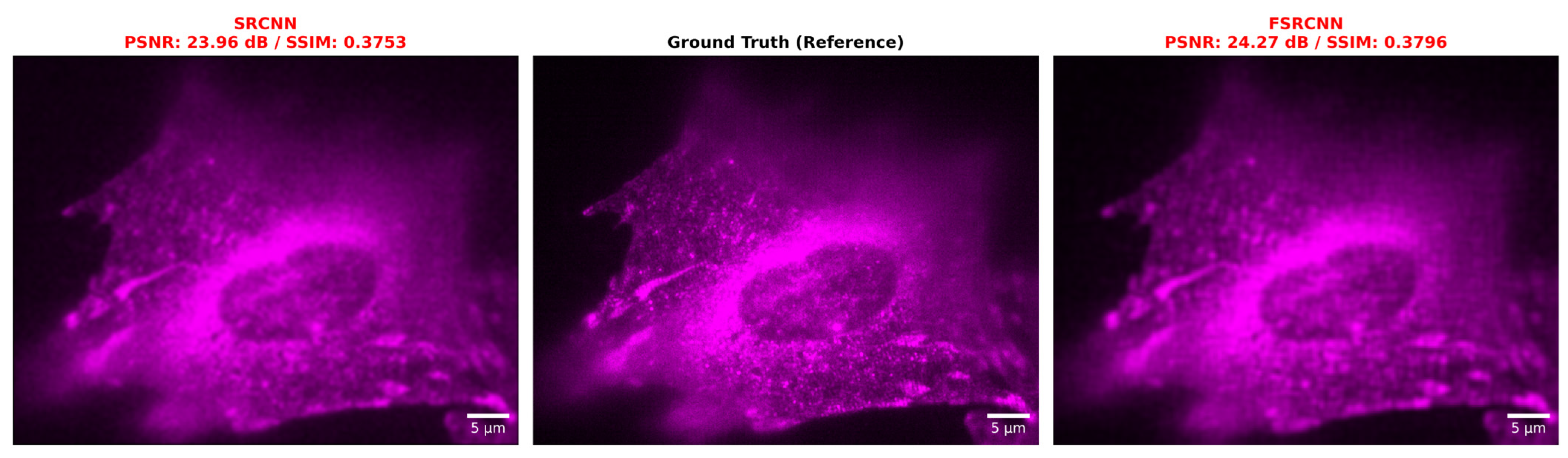
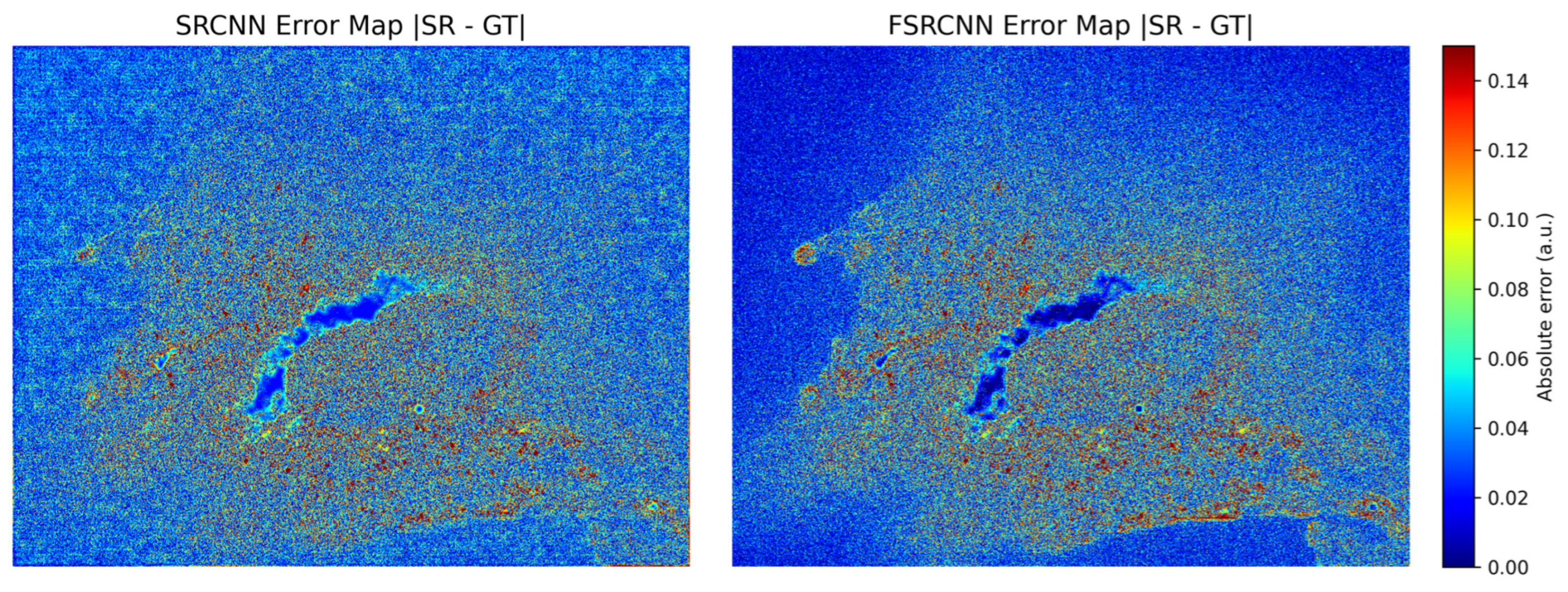
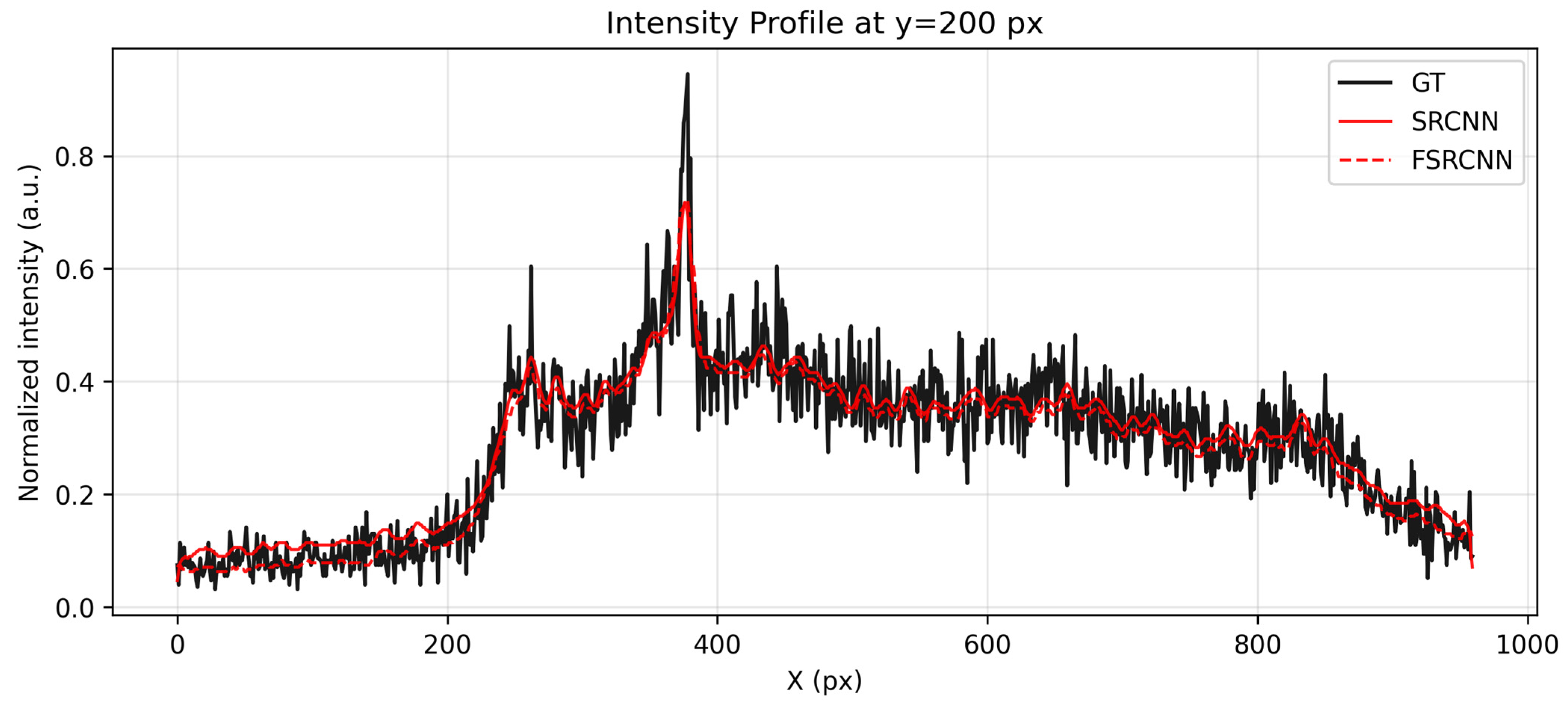
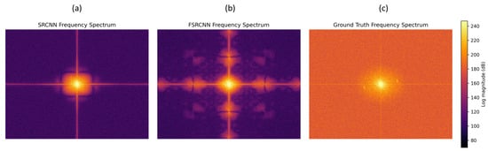
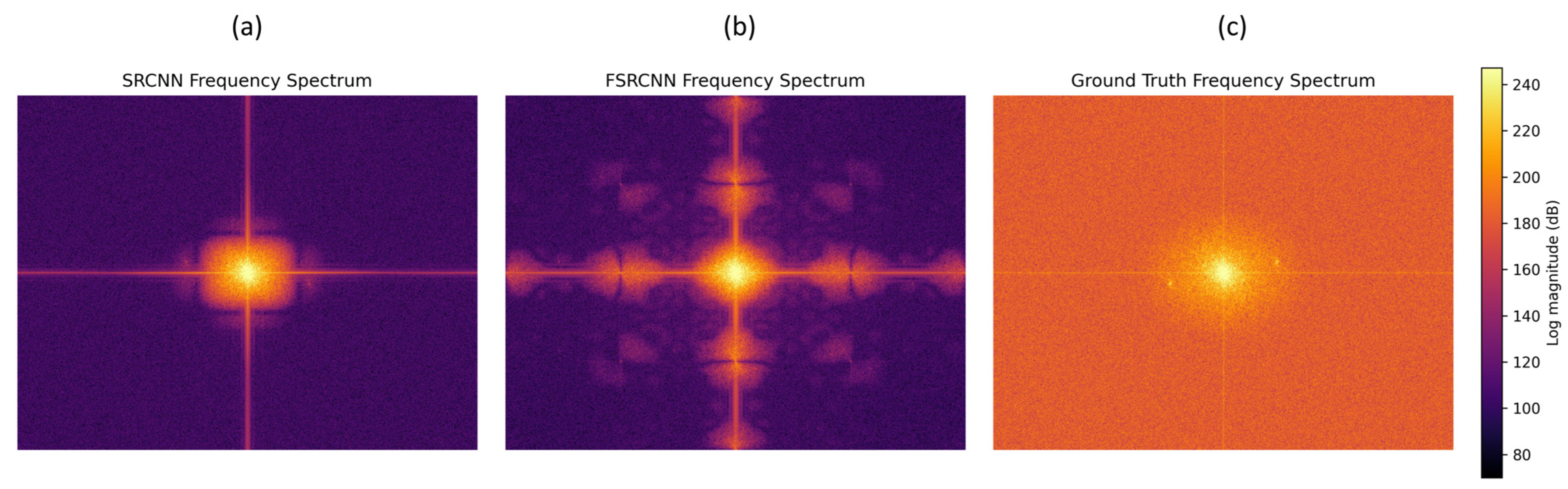
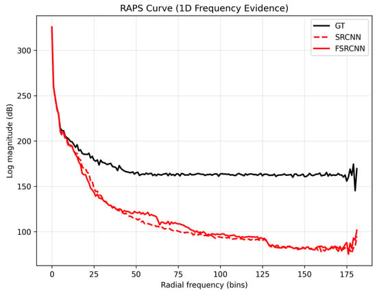
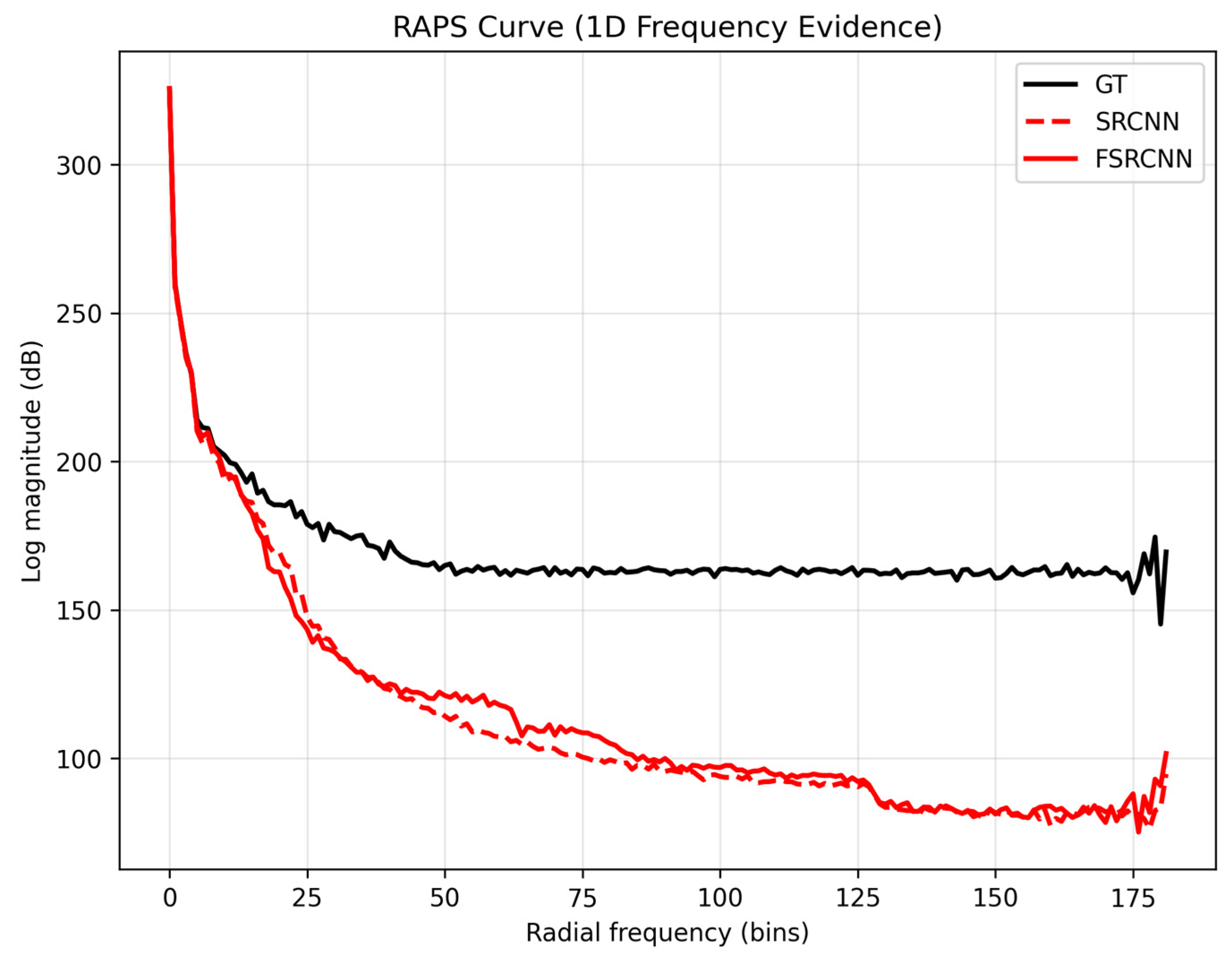
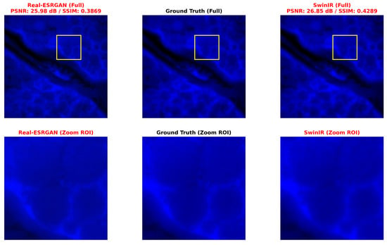
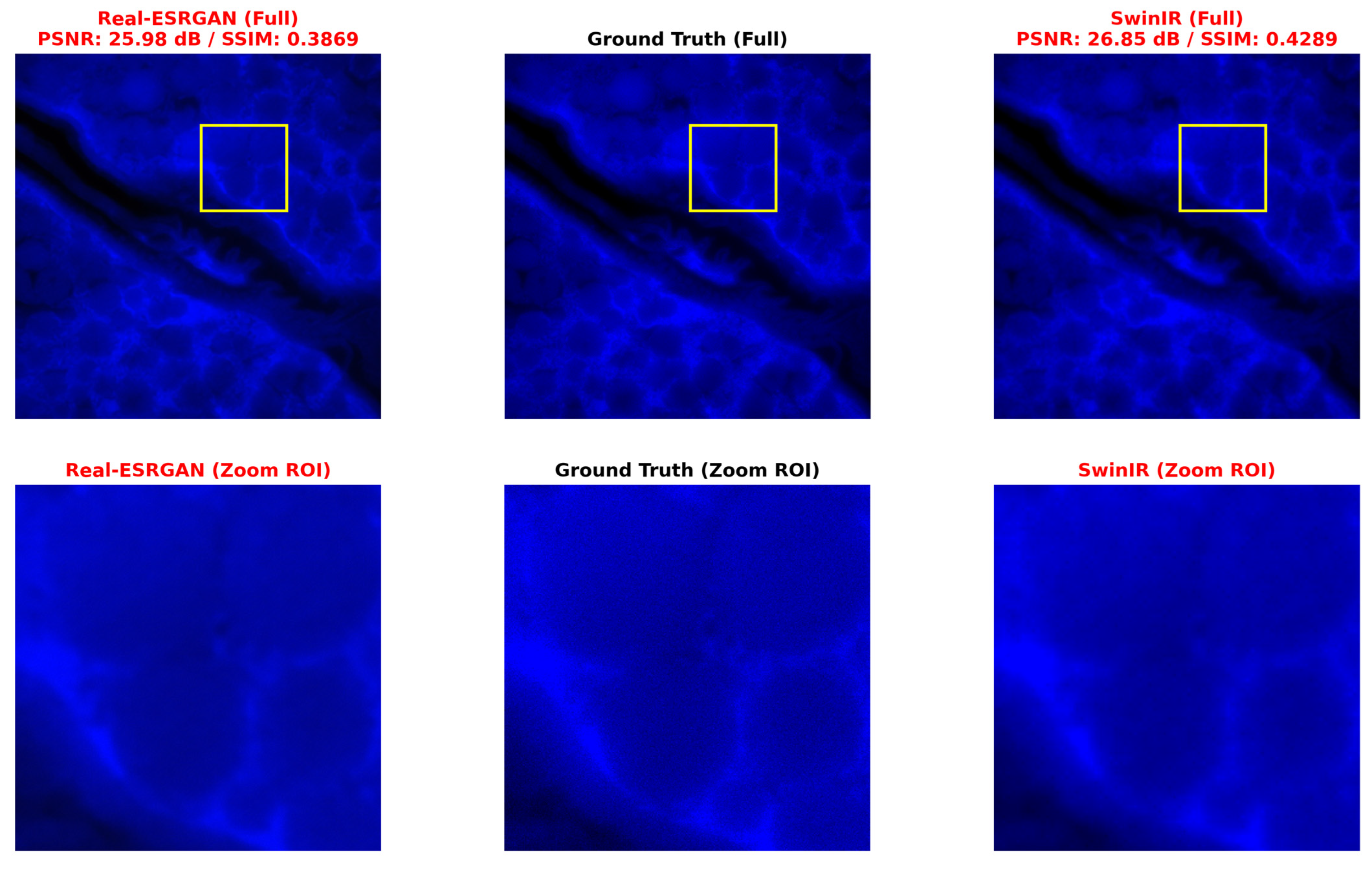
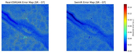
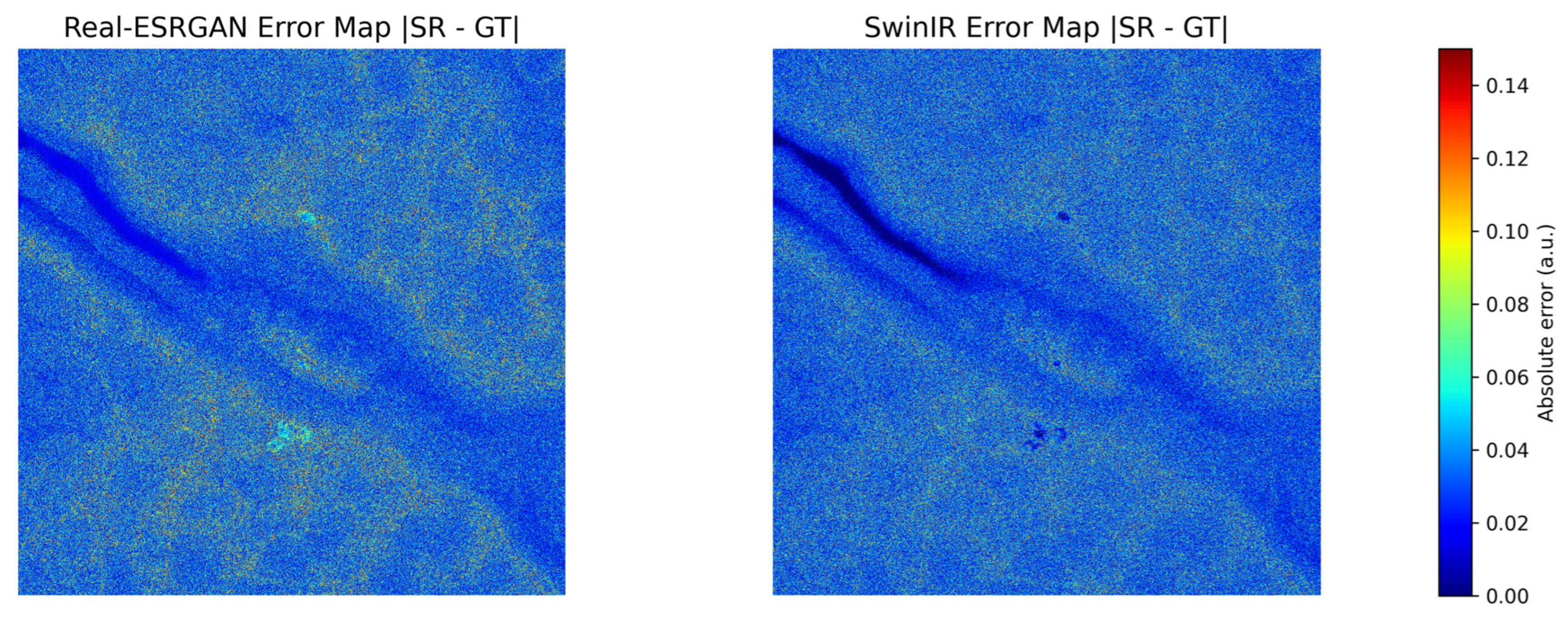
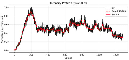
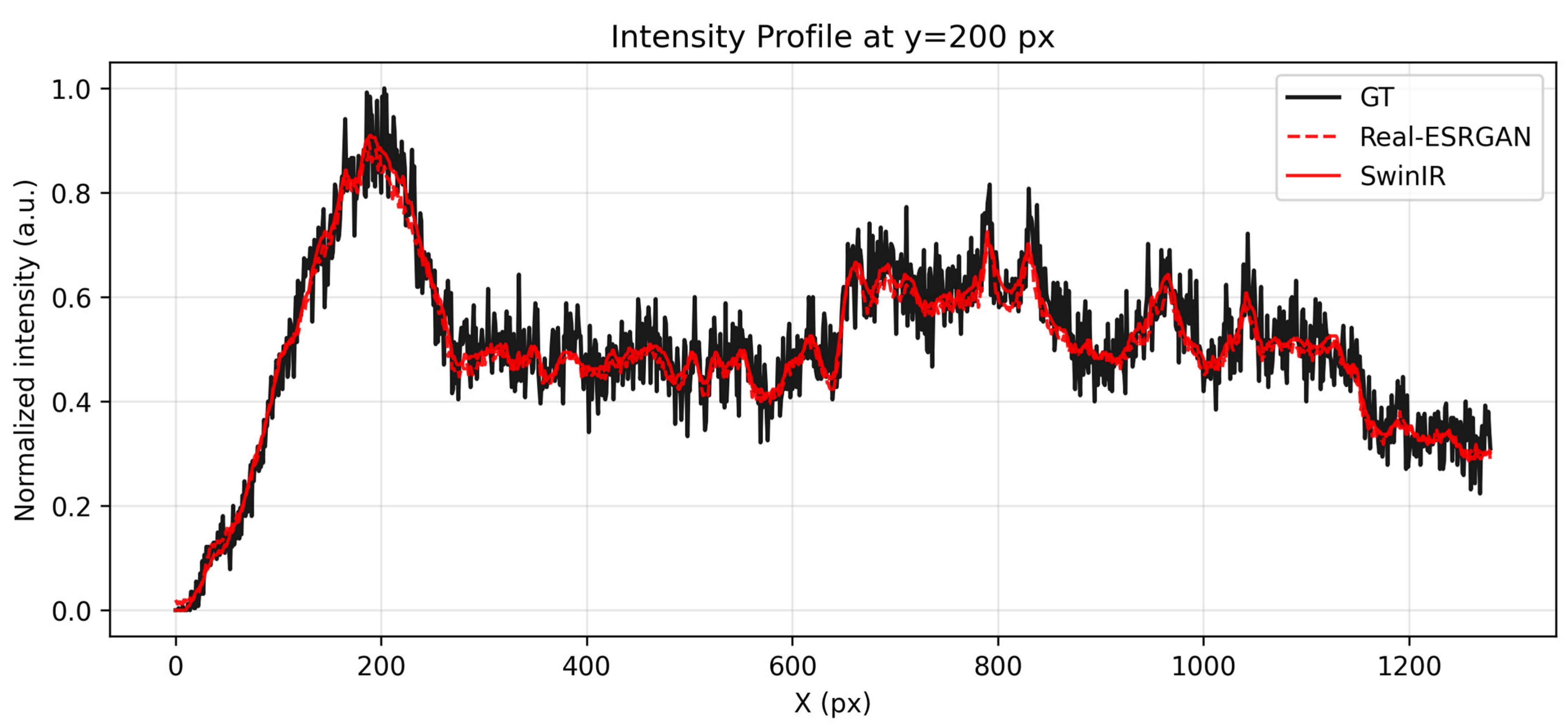
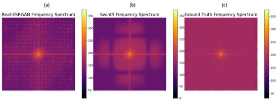
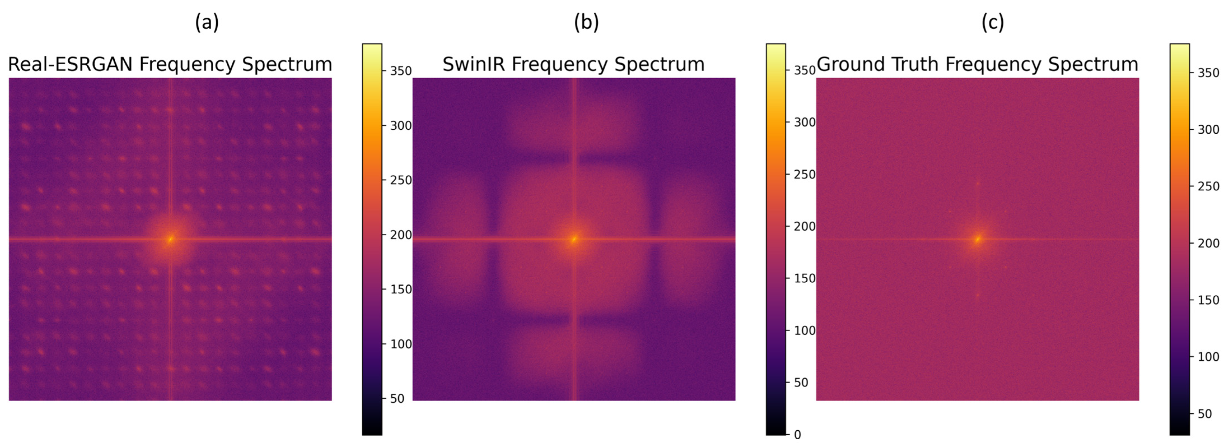
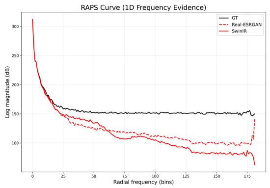
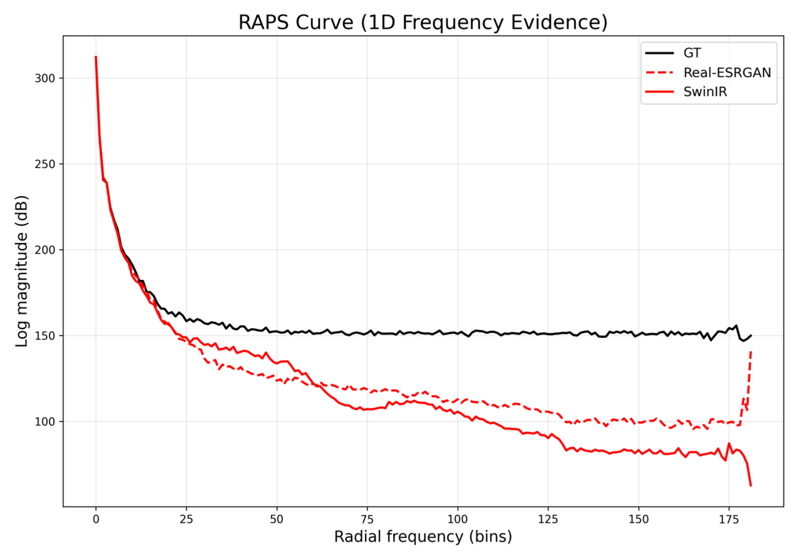
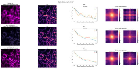
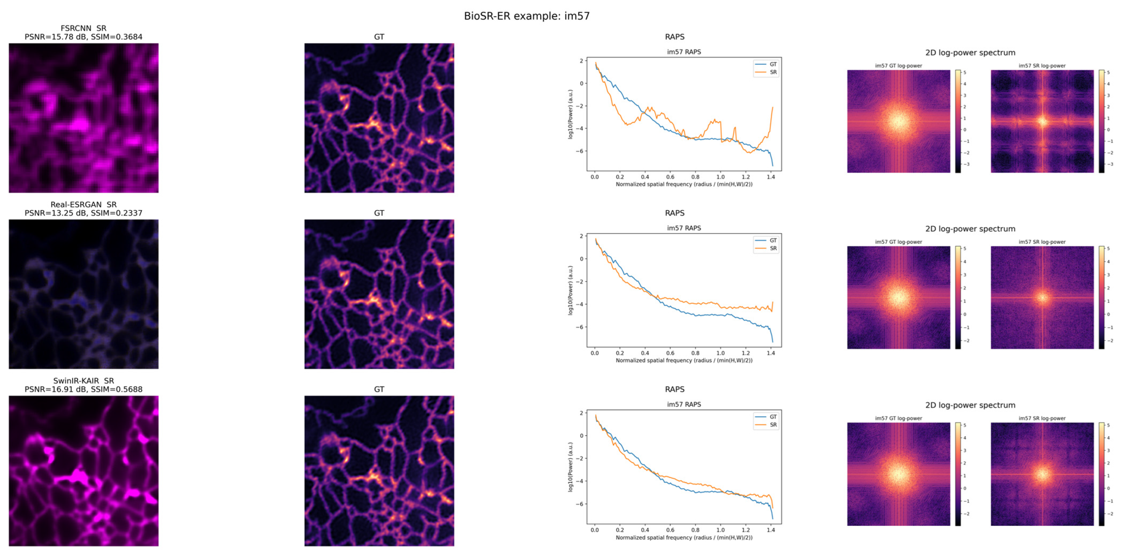

Disclaimer/Publisher’s Note: The statements, opinions and data contained in all publications are solely those of the individual author(s) and contributor(s) and not of MDPI and/or the editor(s). MDPI and/or the editor(s) disclaim responsibility for any injury to people or property resulting from any ideas, methods, instructions or products referred to in the content. |
© 2026 by the authors. Licensee MDPI, Basel, Switzerland. This article is an open access article distributed under the terms and conditions of the Creative Commons Attribution (CC BY) license.