Wavefront Prediction for Adaptive Optics Without Wavefront Sensing Based on EfficientNetV2-S

Abstract

Adaptive optics (AO) aims to counteract wavefront distortions caused by atmospheric turbulence and inherent system errors. Aberration recovery accuracy and computational speed play crucial roles in its correction capability. To address the issues of slow wavefront aberration detection speed and low measurement accuracy in current wavefront sensorless adaptive optics, this paper proposes a wavefront correction method based on the EfficientNetV2-S model. The method utilizes paired focal plane and defocused plane intensity images to directly extract intensity features and reconstruct phase information in a non-iterative manner. This approach enables the direct prediction of wavefront Zernike coefficients from the measured intensity images, specifically for orders 3 to 35, significantly enhancing the real-time correction capability of the AO system. Simulation results show that the root mean square error (RMSE) of the predicted Zernike coefficients for D/r₀ values of 5, 10, and 15 are 0.038λ, 0.071λ, and 0.111λ, respectively, outperforming conventional convolutional neural network (CNN), ResNet50/101 and ConvNeXt-T models. The experimental results demonstrate that the EfficientNetV2-S model maintains good wavefront reconstruction and prediction capabilities at D/r₀ = 5 and 10, highlighting its high precision and robust wavefront prediction ability. Compared to traditional iterative algorithms, the proposed method offers advantages such as high precision, fast computation, no need for iteration, and avoidance of local minima in processing wavefront aberrations.

1. Introduction

Adaptive optics (AO) improves imaging quality by measuring and compensating wavefront errors introduced by the propagation medium in real time. It has been widely used in ground-based telescopes, microscopy, ocular aberration correction, and laser communication [1,2,3,4,5]. A conventional AO system typically consists of a wavefront sensor, a controller, and a wavefront corrector: the sensor measures the distorted wavefront, the controller computes the control signals, and the corrector generates a conjugate phase to cancel aberrations. Despite its effectiveness, this architecture suffers from two major limitations. First, the wavefront-sensing branch usually requires an additional measurement optical path, increasing system complexity, alignment difficulty, and cost. Second, as AO applications expand to scenarios such as free-space optical communication, intracavity aberration correction, and extended-target imaging, the constraints of traditional sensor-based AO increasingly hinder efficiency and practicality. These challenges have motivated the development of wavefront sensorless (WFS-less) AO as an effective alternative [6]. WFS-less AO reconstructs the pupil phase from intensity information using algorithmic inversion and can be broadly categorized into single-image and phase-diversity approaches. Single-image methods infer wavefront errors from one intensity image; however, due to the inherent many-to-one ambiguity in intensity-to-phase mapping, they often exhibit limited accuracy and robustness. Phase-diversity methods use focused and defocused images to uniquely constrain the phase, thereby improving reconstruction fidelity [7]. Nevertheless, conventional WFS-less AO typically relies on iterative optimization and repeated measurements to reach an optimal correction, which reduces correction efficiency and limits deployment in time-critical applications.

In recent years, machine learning—especially data-driven deep learning—has attracted growing interest in AO [8,9]. Early work by Angel et al. [1] employed a three-layer feedforward network to map intensity distributions to Zernike coefficients, enabling piston and tilt correction in multi-telescope systems. Sandler and Barrett [10,11] further demonstrated real-star observations using a backpropagation neural network with focused/defocused image pairs, achieving Zernike coefficient estimation up to the 11th order. However, learning-based prediction under stronger turbulence and higher-order aberration regimes remains challenging, where the intensity patterns become more complex and subtle, and model generalization can degrade. Convolutional neural networks (CNNs) have a strong capacity for learning nonlinear input–output relationships and have achieved outstanding performance in many vision tasks, such as medical imaging [12], street-scene recognition [13], video recognition [14], vehicle detection [15] and microscopy [16]. In WFS-less AO, Nishizaki et al. [17] proposed a CNN to estimate the first 32 Zernike coefficients from a single intensity image. Ma et al. [18] introduced an AlexNet-based approach trained with focused/defocused image pairs and the corresponding coefficients. Yuan et al. [19] fine-tuned EfficientNet using simulated turbulence phase screens and predicted 66 coefficients from a single intensity image, and Yue et al. [20] developed an EfficientNet-B0-based sensorless prediction method using a single degraded focal-plane image. To enhance estimation accuracy, Ma et al. [21] proposed a GoogLeNet-based dual-frame recovery method, and Kok et al. [22] presented a ResNet50-based aberration characterization framework that can further refine predictions with a small number of iterations using phase-diversity images.

Although existing studies have demonstrated the feasibility of deep learning-based wavefront prediction for WFS-less AO, several limitations remain. First, under medium-to-strong turbulence conditions, where high-order aberrations dominate the wavefront distortion, many existing network backbones lack sufficient representational capability to reliably capture fine-grained, high-frequency distortion features from intensity measurements, resulting in increased prediction errors. Second, a number of reported approaches rely on multi-frame inputs and/or iterative refinement strategies, which impose additional acquisition and computational burdens and significantly constrain their applicability in high-speed, real-time AO systems. To address these challenges, this paper adopts EfficientNetV2-S as the backbone network for wavefront prediction in a WFS-less AO framework. A focused–defocused image pair is used as the network input to alleviate the inherent ambiguity of single-intensity measurements, while the corresponding Zernike coefficients are directly regressed in a single forward pass, thereby avoiding iterative optimization and enabling high-speed operation.

The selection of EfficientNetV2-S is motivated by both architectural and practical considerations specific to WFS-less AO. Compared with conventional CNN backbones, the EfficientNet family achieves superior accuracy–efficiency trade-offs through compound scaling of network depth and width, which is particularly advantageous for modeling turbulence-induced intensity distortions across multiple spatial scales. Compared with EfficientNetV1, EfficientNetV2 introduces Fused Mobile Inverted Bottleneck Convolution (Fused-MBConv) blocks that enhance low-level feature extraction and significantly improve training stability and efficiency, which is critical for learning high-order aberration representations from large-scale simulated datasets. Furthermore, the incorporation of squeeze-and-excitation (SE) attention strengthens channel-wise feature discrimination, enabling the network to better distinguish subtle intensity variations caused by complex atmospheric turbulence. Among the EfficientNetV2 variants, the S version provides a balanced compromise between representational capacity and computational complexity. While larger variants such as EfficientNetV2-M and -L offer increased model capacity, they incur substantially higher computational and memory costs, which are unnecessary for the present task and detrimental to real-time deployment. In contrast, EfficientNetV2-S retains sufficient modeling capability for high-order aberration prediction while maintaining a compact parameter size and low inference latency, making it well suited for deployment on embedded platforms such as NVIDIA Jetson. These characteristics render EfficientNetV2-S particularly appropriate for medium-to-strong turbulence conditions in WFS-less AO systems, where both robust nonlinear fitting and real-time performance are essential.

In this work, EfficientNetV2-S is compared with several representative architectures, including a conventional CNN, ResNet50/101, and ConvNeXt-T (Tiny), to evaluate wavefront prediction performance. Simulation and experimental results demonstrate that EfficientNetV2-S consistently achieves superior wavefront reconstruction accuracy and improved image restoration quality across different turbulence conditions, indicating its effectiveness and efficiency for deep learning-based wavefront prediction in WFS-less AO systems.

2. Materials and Methods

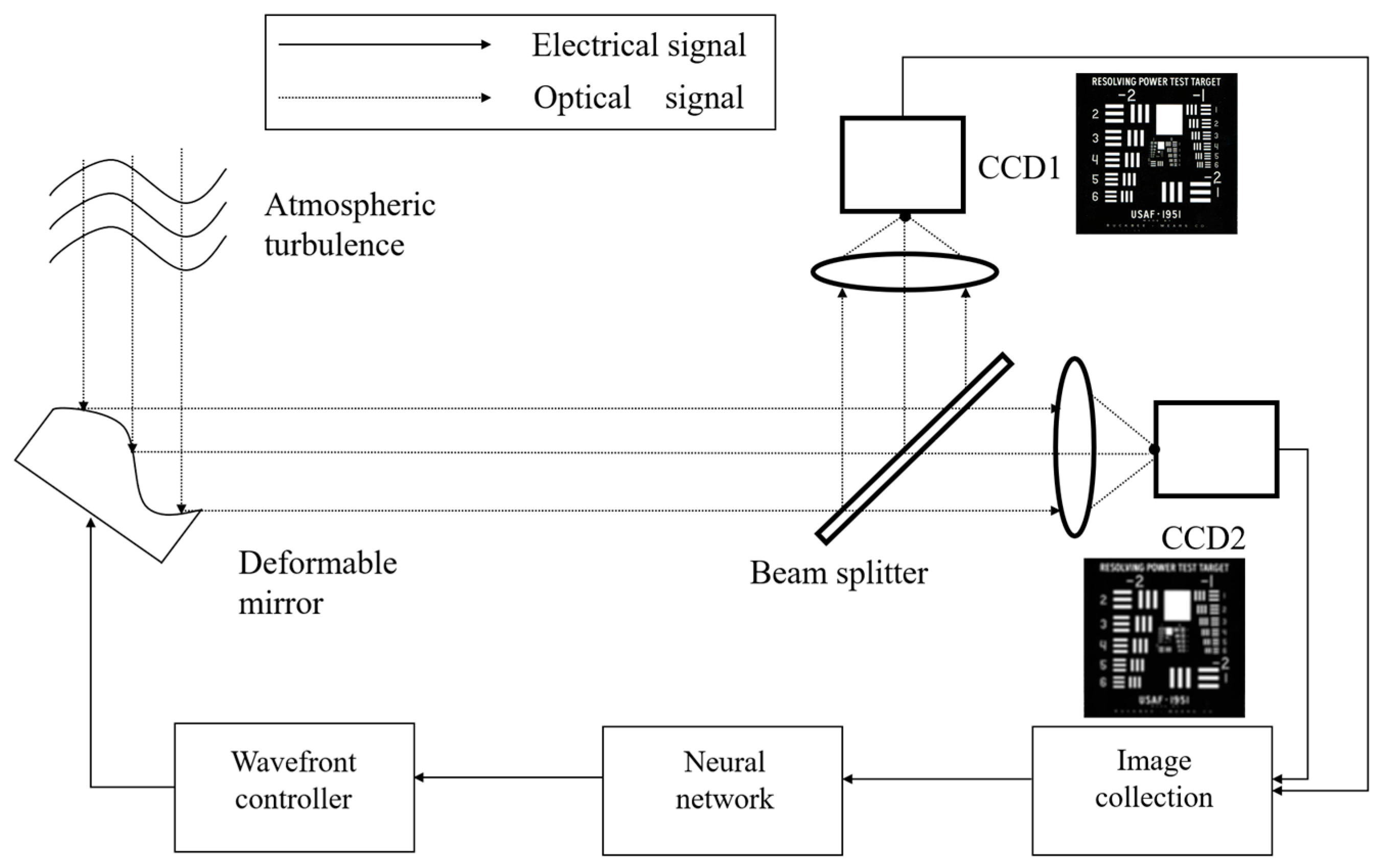
The schematic diagram of the WFS-less AO system based on deep learning is shown in Figure 1. The system mainly comprises a wavefront correction element (deformable mirror, DM), optical lenses, high-speed scientific cameras (CCD1 and CCD2), and a wavefront control module. Collimated light emitted from the source is distorted after propagating through atmospheric turbulence. The aberrated beam is then reflected by the DM and divided into two optical paths by a beam splitter. One beam is focused by a lens onto CCD1, where the focal-plane intensity distribution is recorded. The other beam, after an artificially introduced defocus, is incident on CCD2 to capture the intensity image at the defocused plane. The intensity images from the two CCDs are sent to the “Image collection” unit and combined as input data, which are then processed through a neural network to obtain the corresponding Zernike coefficients. The wavefront controller calculates the driving electrical signal for the DM based on these coefficients, and the signal returns to the DM via the solid line path to achieve closed-loop compensation of the wavefront aberration. In this way, the system can perform efficient wavefront correction using both in-focus and out-of-focus information without the need for a dedicated wavefront sensor.

Atmospheric turbulence phase screens are typically generated using two main approaches. The first is the power spectrum inversion method, which reconstructs the phase distribution from the turbulence power spectral density. The second is the Zernike polynomial expansion method, in which the phase is represented as a weighted sum of orthogonal Zernike basis functions. The power spectrum inversion approach primarily provides accurate representation of high-frequency components, while the Zernike polynomial expansion method is more widely adopted in practical applications for constructing atmospheric turbulence phase screens. This paper employs the Zernike polynomial expansion method to generate turbulence phase screens and constructs a numerical simulation model for WFS-less AO, thereby producing degraded target images and the corresponding Zernike aberration coefficients to form the training dataset for the network. Under atmospheric turbulence with different strengths, a randomly distorted wavefront $\phi (x,y)$ can be expressed as:

$$\phi (x,y)={\displaystyle \sum _{i=1}^M{a}_i}{z}_i(x,y)$$

(1)

In Equation (1), $\phi (x,y)$ represents the generated phase; $a_i$ is the coefficient of the $i$-th Zernike polynomial; $z_i(x,y)$ is the $i$-th Zernike polynomial; and $M$ is the Zernike order. When an aberrated plane wave passes through a lens, it generates an incident initial light field $W_0(x,y)$, which is imaged on CCD1 and CCD2 in the far field, obtaining the intensity distribution at the focal and defocused planes. By performing a Fourier transform on the incident light field $W_0(x,y)$, the complex amplitude of the light field at the focal plane can be reconstructed, that is, the complex amplitude $W_1\left(f_x,f_y\right)$ of the light field at the focal plane can be expressed as:

$$W_1\left(f_x,f_y\right)=Q_1\mathcal{F}\left\{W_0(x,y)\right\}$$

(2)

In Equation (2), $Q_1$ represents a complex constant, and $\mathcal{F}$ represents the Fourier transform. The complex amplitude of the light field $W_2\left(f_x,f_y\right)$ at the defocused plane can be expressed as:

$$W_2\left(f_x,f_y\right)=Q_2\mathcal{F}\left\{W_0(x,y)\exp \left[-\mathrm{i}{\phi }_{\mathrm{d}}(x,y)\right]\right\}$$

(3)

In Equation (3), $Q_2$ represents a complex constant, and ${\phi }_{\mathrm{d}}(x,y)$ represents the defocus-induced phase term. The intensity at the focal and defocused planes is the squared magnitude of the complex optical field, as given in Equation (4):

$$I_1(x,y)={\left|W_1\left(f_x,f_y\right)\right|}^2$$

(4a)

$$I_2(x,y)={\left|W_2\left(f_x,f_y\right)\right|}^2$$

(4b)

The intensity images acquired at the focal and defocused planes contain information about the wavefront aberrations of the optical system. To retrieve these aberrations, a neural network is employed to extract the corresponding Zernike coefficients from the recorded images, thereby enabling reconstruction of the system wavefront. To achieve this, the neural network is trained offline using a large number of samples, where the input consists of intensity images captured on the CCD under static distorted wavefronts, and the output corresponds to the associated Zernike coefficients. The wavefront reconstruction process based on a neural network can be viewed as a nonlinear mapping: by inputting two intensity images, the network outputs the Zernike coefficients of the corresponding distorted wavefront. After training the model, $\left\{a_1,a_2,\cdots ,a_M\right\}$ can be expressed as Equation (5), in which $f_{\mathrm{NN}}(\cdot )$ represents the neural network model.

$$\left\{a_1,a_2,\cdots ,a_M\right\}=f_{\mathrm{NN}}\left[I_1(x,y),I_2\left(x,y_y\right)\right]$$

(5)

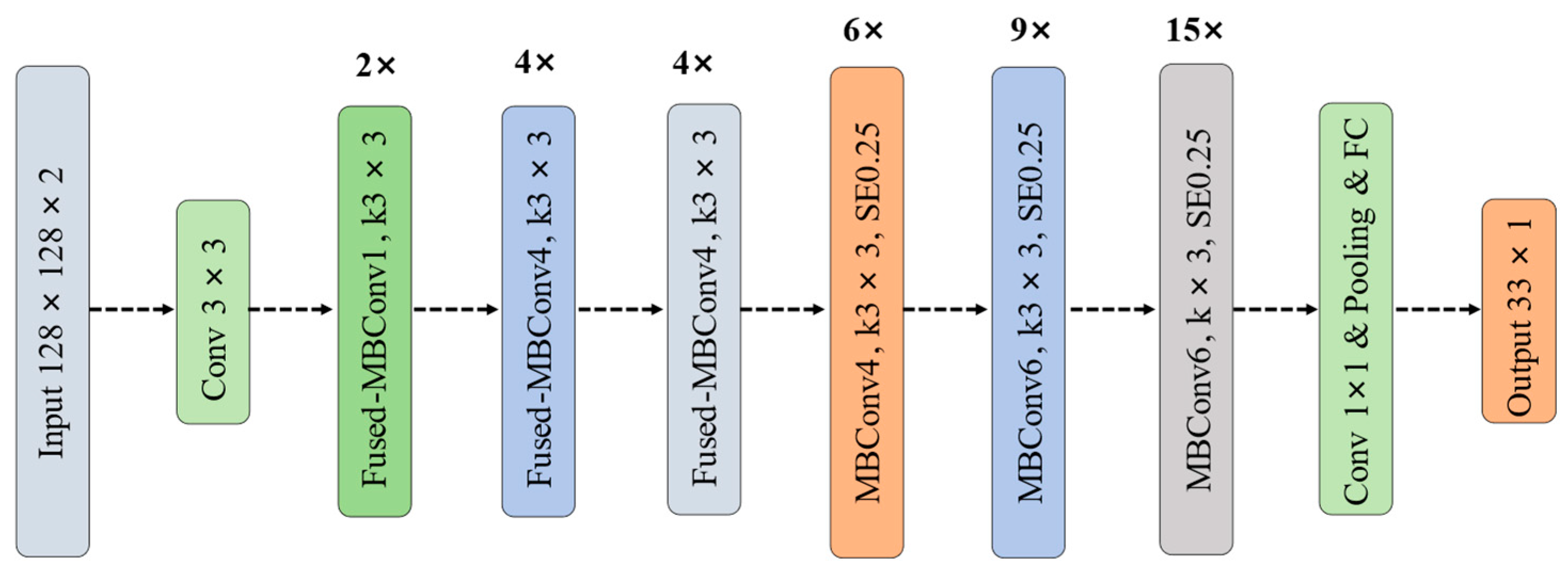
This paper proposes a WFS-less AO correction method based on the EfficientNetV2-S model. EfficientNetV2 is a next-generation CNN family proposed by Google in 2021 [23]. Through the use of neural architecture search (NAS) and compound scaling, it significantly improves training speed while maintaining parameter efficiency. EfficientNetV2-S, a lightweight variant in the EfficientNetV2 family, adopts compound scaling to jointly scale the network depth, width, and input resolution, thereby achieving a balanced trade-off between computational efficiency and model performance. Its overall architecture is shown in Figure 2 and

Table 1. EfficientNetV2-S network model parameters table [23].

Stage	Operator	Stride	Channels	Layers
0	Conv3 × 3	2	24	1
1	Fused-MBConv1, k3 × 3	1	24	2
2	Fused-MBConv4, k3 × 3	2	48	4
3	Fused-MBConv4, k3 × 3	2	64	4
4	MBConv4, k3 × 3, SE0.25	2	128	6
5	MBConv6, k3 × 3, SE0.25	1	160	9
6	MBConv6, k3 × 3, SE0.25	2	256	15
7	Conv1 × 1 & Pooling & FC	-	1280	1

.

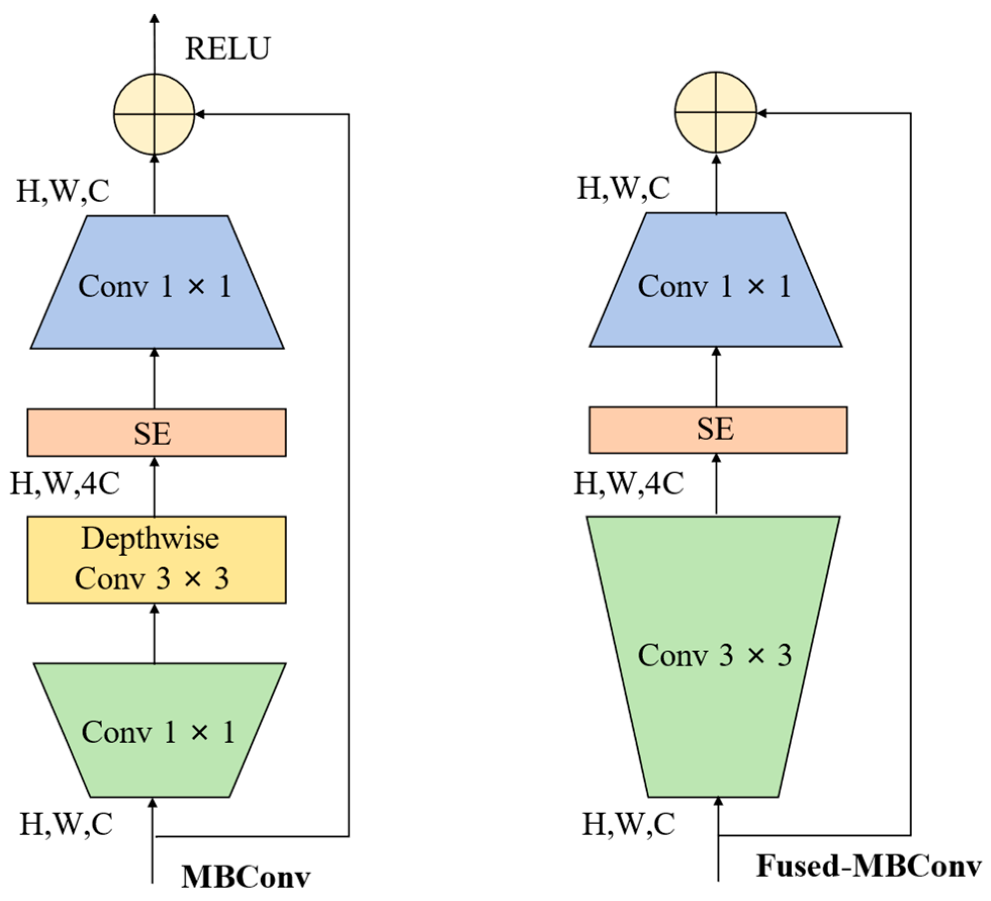
EfficientNetV2 is organized into multiple stages, with each stage built upon the Fused-MBConv block as the fundamental unit. Compared with the original EfficientNet, EfficientNetV2 introduces three key improvements to enhance training efficiency and feature representation. First, the Fused-MBConv module, as illustrated in Figure 3, replaces the depthwise 3 × 3 convolution and the 1 × 1 expansion convolution in Mobile Inverted Bottleneck Convolution (MBConv) with a single standard 3 × 3 convolution, which simplifies the computation graph and better exploits the parallelism of GPUs/TPUs, thereby significantly improving training throughput with only a slight increase in FLOPs. Second, the SE attention module adaptively recalibrates channel-wise feature responses by computing channel weights in the shortcut branch and applying them to the main-branch features through element-wise multiplication, effectively enhancing channel dependencies with negligible parameter overhead. Third, Drop-Connect is adopted instead of conventional Dropout by randomly dropping hidden layer connections rather than outputs, which further alleviates overfitting without introducing additional inference cost. Owing to these advantages, the lightweight variant EfficientNetV2-S is selected in this work as the backbone network to achieve a favorable trade-off between computational efficiency and representation capability. The detailed configurations of the EfficientNetV2 family are summarized in

Table 2. EfficientNetV2 series network configuration [23].

EfficientNetV2	S		M		L
	Min	Max	Min	Max	Min	Max
Image size	128	300	128	380	128	380
RandAugment	5	15	5	20	5	25
Mixup alpha	0	0	0	0.2	0	0.4
Dropout	0.1	0.3	0.1	0.4	0.1	0.5

.

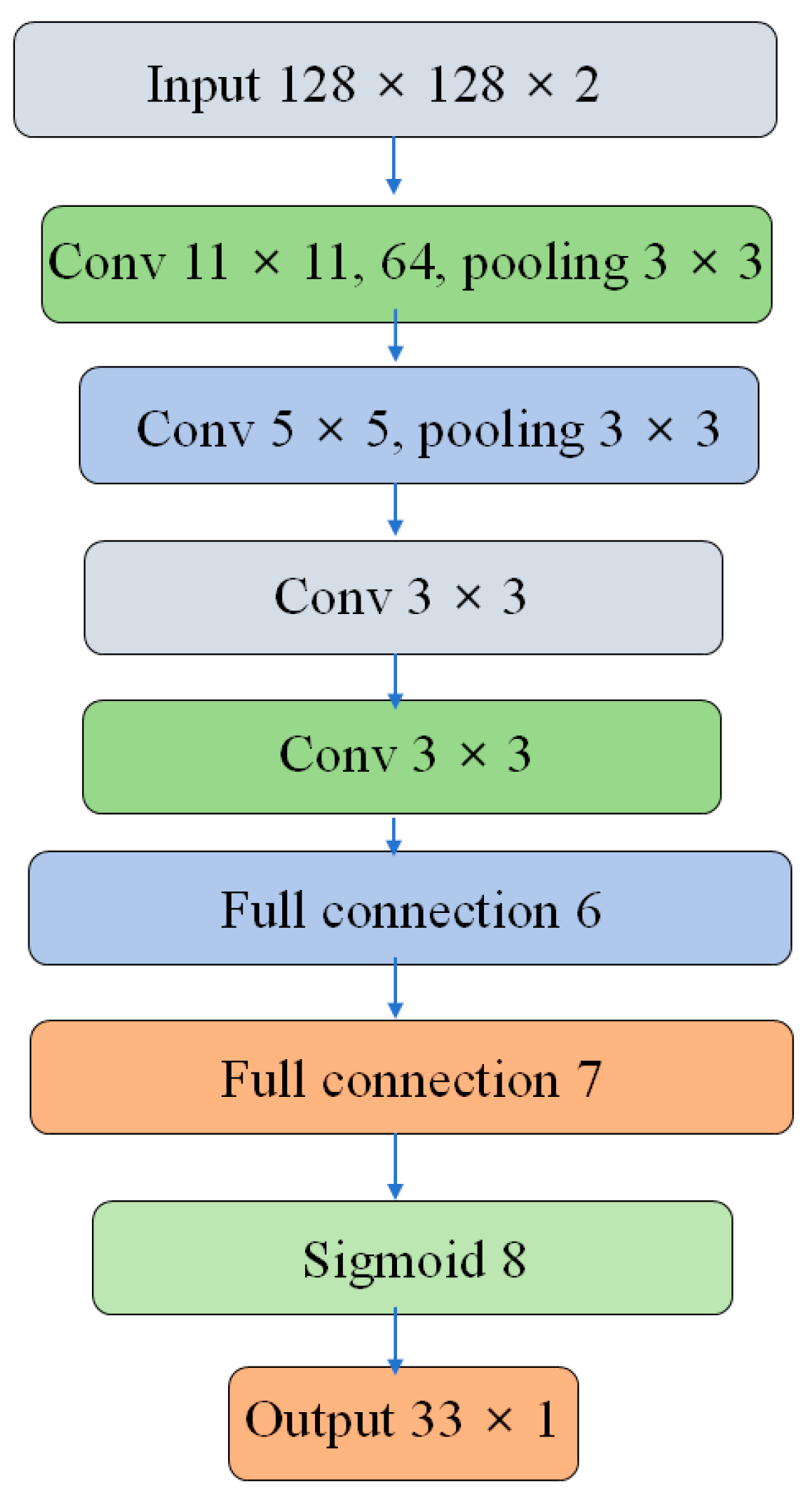
To verify the performance of EfficientNetV2-S for wavefront prediction, several representative network architectures are selected for comparison, including a conventional CNN, ResNet50, ResNet101, and ConvNeXt-T. The structural characteristics and key configurations of these counterpart networks are described as follows. The conventional CNN adopted in this study is composed of an eight-layer architecture, as illustrated in Figure 4. Within the network, a “3 × 3” notation denotes the convolution kernel size, while “64” specifies the number of kernels employed in the corresponding convolutional layer. The stride parameter defines the step length of each convolution operation. To improve nonlinear representation capability, the ReLU activation function is applied after every layer. The output layer consists of 33 neurons, corresponding to the prediction of 33 Zernike coefficients from the 3rd to the 35th modes, excluding the piston and tip/tilt components.

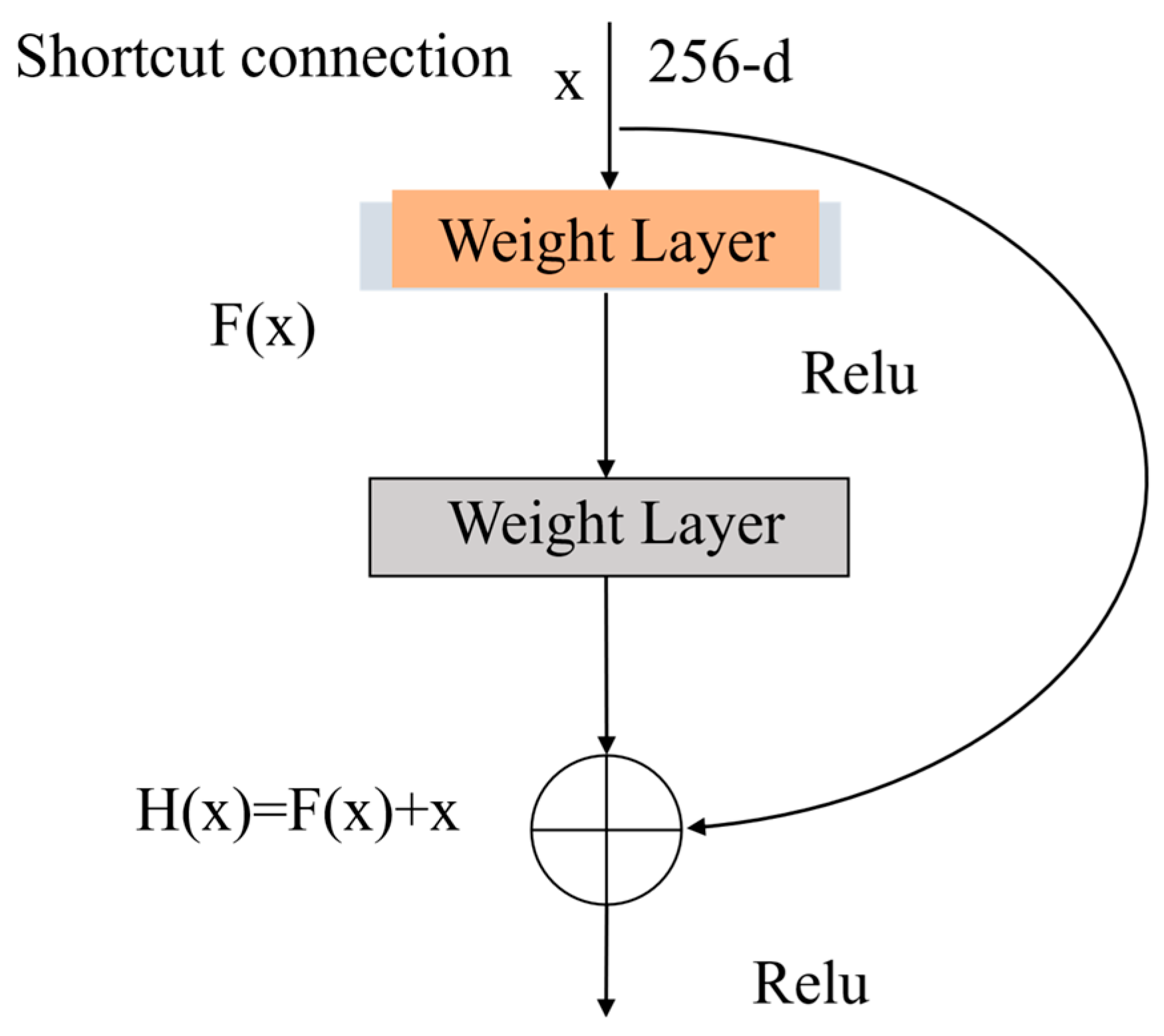
Residual networks (ResNet) have developed from early 18-layer configurations to very deep architectures containing up to 152 layers. In principle, increasing network depth enables the extraction of more complex and abstract features, potentially enhancing model performance. However, excessive nonlinear transformations in deep networks may lead to progressive loss of feature information, resulting in performance degradation as depth increases. To overcome this limitation, ResNet introduces residual blocks that employ shortcut connections to implement identity mappings. These connections allow the network to preserve feature information better, enhance sensitivity to data variations, and facilitate the construction of robust mappings from image inputs to numerical outputs. Moreover, residual learning effectively alleviates the vanishing gradient problem associated with deep architectures, thereby preventing network degradation and improving prediction accuracy. The detailed ResNet architecture is illustrated in Figure 5. As the target output of this study consists of 33 Zernike coefficients, only the final fully connected layer is adjusted to produce 33 output nodes. The residual module is shown in Figure 6. Through the “shortcut connection”, the input is directly passed to the output $\mathrm{H}\left(\mathrm{x}\right)=\mathrm{F}\left(\mathrm{x}\right)+\mathrm{x}$, resulting in $\mathrm{H}\left(\mathrm{x}\right)=\mathrm{x}$ when $\mathrm{F}\left(\mathrm{x}\right)=0$. $\mathrm{F}\left(\mathrm{x}\right)$ denotes the residual function, which represents the residual mapping to be learned [24]. Therefore, the training objective is to make the residual result close to 0, thus avoiding the accuracy degradation caused by deepening the network. 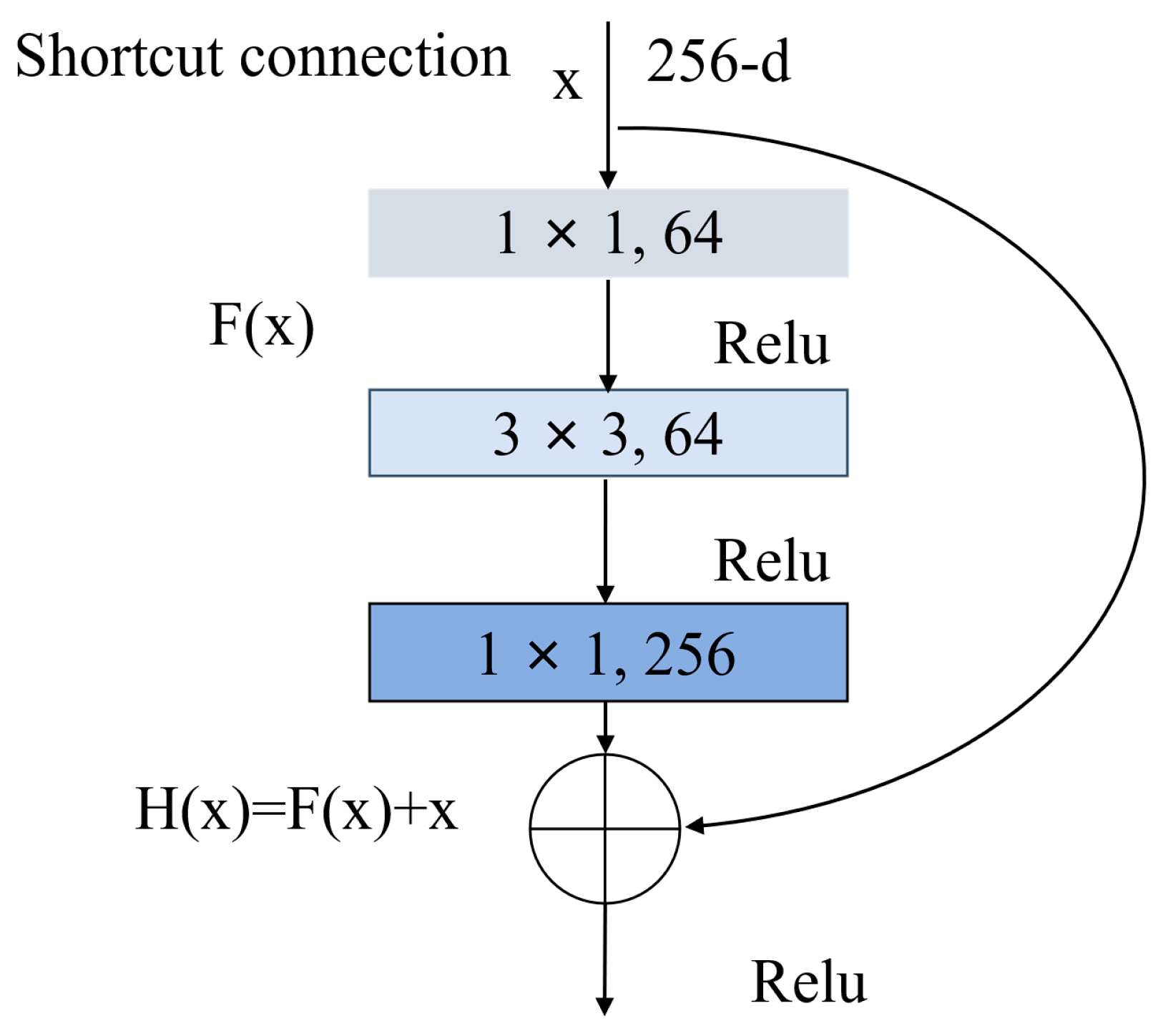Figure 7 depicts the specific building block for ResNet50/101.

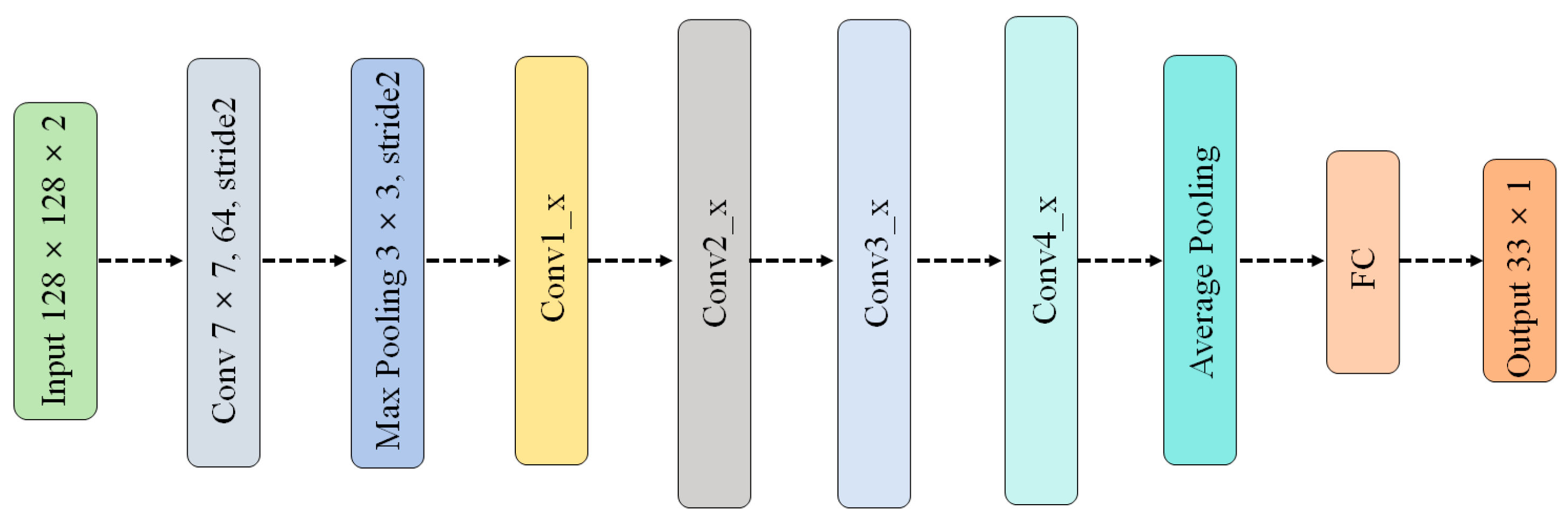
ConvNeXt [25] is a novel and efficient CNN model proposed by the Facebook AI Research (FAIR) team in 2022. Compared with traditional convolutional networks, ConvNeXt significantly improves training and inference performance while maintaining structural efficiency, by incorporating a series of advanced design choices such as larger convolution kernels and hierarchical architectures. The ConvNeXt model adopts a simplified “modular” design. Within the ConvNeXt family, ConvNeXt-T serves as a lightweight baseline model targeting high-efficiency application scenarios, and its architecture is illustrated in Figure 8.

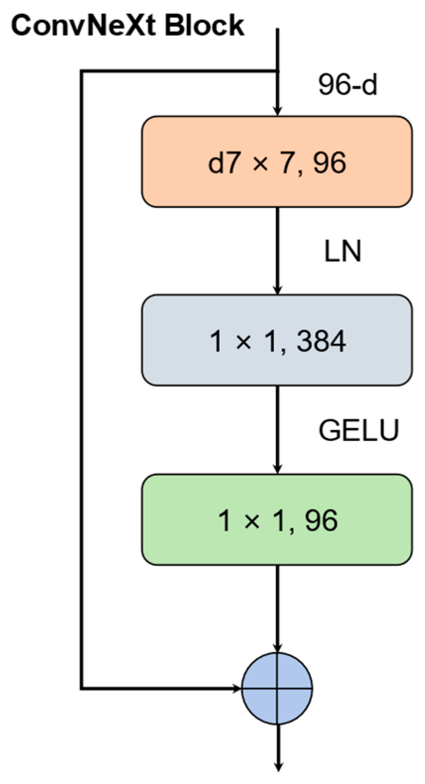
The model stacks 3, 3, 9, and 3 ConvNeXt blocks in its four stages, respectively, and progressively reduces the spatial resolution while increasing the channel dimensionality, thereby achieving a favorable balance between computational cost and representational capacity. The architecture of a ConvNeXt block is illustrated in Figure 9. While maintaining a relatively small model size, ConvNeXt-T demonstrates excellent accuracy and inference efficiency across a variety of visual tasks. Compared with larger ConvNeXt-S, B, and L models, ConvNeXt-T significantly reduces computational complexity and memory overhead at the cost of only a minor drop in peak accuracy, resulting in faster inference speed and higher energy efficiency.

According to the Kolmogorov turbulence theory, the covariance matrix $C$ of the Zernike polynomial coefficient vector $A=\left\{a_1,a_2,\cdots ,a_M\right\}$ can be obtained, which is expressed as:

$$〈a_i{a}_j〉=c_{ij}{\left({\displaystyle \frac{D}{r_0}}\right)}^{5/3}$$

(6)

In Equation (6), $c_{ij}$ represents the covariance coefficient; $a_i$ and $a_j$ are the $i$-th and $j$-th Zernike coefficients, respectively; $D$ is the aperture diameter; $r_0$ is the atmospheric coherence length; $r_0={\left[0.423k^2{\displaystyle {\int }_0^L{C}_n^2(z)\mathrm{d}z}\right]}^{-3/5}$; $k={\displaystyle \frac{2\pi }{\lambda }}$; $\lambda$ is the wavelength; $C_n^2(z)$ is the refractive-index structure constant along the propagation path; and $L$ is the propagation distance. The Zernike polynomial coefficient vector $A$ can be obtained using the Karhunen–Loève (KL) polynomials.

$$\left\{\begin{array}{l}C=VS{V}^{\mathrm{T}}\hfill \\ A=VB\hfill \end{array}\right.$$

(7)

In Equation (7), $S$ is a diagonal matrix, $V$ is the coefficient matrix of the KL polynomials with the Zernike basis, and $B$ is the corresponding vector of KL coefficients. Using Equation (1) and the Zernike coefficient vector statistically generated according to the Kolmogorov turbulence spectrum, atmospheric turbulence-distorted wavefronts can be synthesized. In this study, three datasets with D/r₀ = 5, 10, 15 were prepared for training and testing.

By simulating the optical system together with atmospheric turbulence effects, a large and reliable dataset is generated, consisting of degraded intensity images and their corresponding Zernike coefficients. Specifically, 15,000 randomly generated sets of Zernike coefficients $\left\{a_1,a_2,\cdots ,a_M\right\}$ and the associated intensity images $I_1(x,y)$ and $I_2(x,y)$ are used for network training, while an additional 1000 independently generated samples are reserved for testing. The training and test datasets are strictly non-overlapping. The proposed model is trained using the generated datasets, and its learning performance is evaluated based on the loss function. In this study, the L1 loss between the predicted and ground-truth Zernike coefficients is adopted, which is defined as:

$$f_{\mathrm{loss} }={\displaystyle \sum _{i=1}^M\left|a_{true,i}-a_{predict,i}\right|}$$

(8)

In Equation (8), $a_{true,i}$ is the true value of the $i$-th Zernike coefficient, and $a_{predict,i}$ is the predicted value of the $i$-th Zernike coefficient. Subsequently, the network model is iteratively optimized using the backpropagation algorithm. After each training epoch, the updated model is evaluated on a validation set to monitor its generalization performance. Based on the validation results, the training process is further refined to obtain the final optimized prediction model. In this paper, the effectiveness of the proposed method is validated through comparative experiments with other neural network models under identical datasets and experimental conditions.

3. Results and Discussion

3.1. Numerical Simulation

All simulations and experiments were conducted using the PyTorch deep learning framework (PyTorch 2.6.0+cu124). The figures were generated using MATLAB R2024b. The computer used for the experiment was running Windows 11, with the following hardware configuration: Intel Core i9-10900K CPU (3.7 GHz), 32 GB DDR4 RAM, and an NVIDIA GeForce RTX 2080Ti GPU. We constructed conventional CNN, ResNet50/101, ConvNeXt-T and EfficientNetV2-S networks, and trained these networks based on the established dataset. Each network was trained for 400 epochs with a batch size of 64. The loss function used was the L1 loss of the Zernike coefficients. A custom cosine annealing learning rate decay strategy was used, and the Adam optimizer was employed. The specific parameters of the four convolutional neural networks are shown in

Table 3. Specifications of the neural network.

Neural Network	Input	Epochs	Optimizer	Batch Size	Loss Function
CNN	128 × 128	400	Adam	64	L1
ResNet50/101	128 × 128	400	Adam	64	L1
ConvNeXt-T	128 × 128	400	Adam	64	L1
EfficientNetV2-S	128 × 128	400	Adam	64	L1

.

To further investigate the contribution of individual modules in the EfficientNetV2-S architecture, ablation experiments were conducted by removing the SE attention module and by replacing Fused-MBConv blocks with standard MBConv blocks. The L1 loss and the Zernike Root Mean Square Error (ZRMSE) were employed as evaluation metrics to quantify the prediction accuracy of the Zernike coefficients. For a more intuitive comparison of algorithm performance, the L1 loss function was scaled by a factor of 5000. The ZRMSE is defined in Equation (9).

$$ZRMSE=\sqrt{{\displaystyle \frac{1}{M}}{\displaystyle \sum _{i=1}^M{\left(a_{true,i}-a_{predict,i}\right)}^2}}$$

(9)

The experiments were conducted under two different turbulence conditions, D/r₀ = 5 and D/r₀ = 10, to examine model performance across different turbulence strengths, and the corresponding results are summarized in

Table 4. Performance comparison of ablation variants under D/r₀ = 5.

Model	L1 Loss	ZRMSE
Baseline	109	0.038λ
Variant 1	137	0.047λ
Variant 2	208	0.068λ

and

Table 5. Performance comparison of ablation variants under D/r₀ = 10.

Model	L1 Loss	ZRMSE
Baseline	208	0.071λ
Variant 1	228	0.077λ
Variant 2	294	0.091λ

. Specifically, the model without the SE attention module is denoted as “Variant 1”, while the model in which Fused-MBConv is replaced by standard MBConv is denoted as “Variant 2”. These ablation studies aim to elucidate the individual contributions of the SE attention and Fused-MBConv modules to the overall prediction performance, particularly under varying turbulence conditions.

Under D/r₀ = 5, the experimental results indicate that there are differences in model performance, especially with the removal of the SE module or the replacement of Fused-MBConv, which have a certain impact on model accuracy. Specifically, removing the SE module leads to a slight increase in L1 loss and ZRMSE, indicating that this module plays a role in enhancing model accuracy. A more noticeable change occurs when Fused-MBConv is replaced with MBConv, resulting in a significant drop in performance. This is especially evident in weaker turbulence conditions, where Fused-MBConv plays a particularly important role in improving feature extraction and convolution efficiency.

When the turbulence intensity increases to D/r₀ = 10, L1 loss and ZRMSE for all models show a noticeable increase, reflecting the more complex impact of wavefront aberrations on model prediction under stronger turbulence conditions. Under these conditions, the effect of removing the SE module becomes more pronounced, and performance further declines. The performance degradation becomes even more evident when Fused-MBConv is replaced by the standard MBConv. In strong turbulence environments, standard MBConv may not effectively handle high-order aberrations, leading to performance deterioration.

Overall, the increase in turbulence intensity significantly affects model performance, and removing or replacing key modules such as the SE module and Fused-MBConv leads to a notable decline in accuracy. This indicates that these modules are crucial for the stability and accuracy of the model under different turbulence conditions.

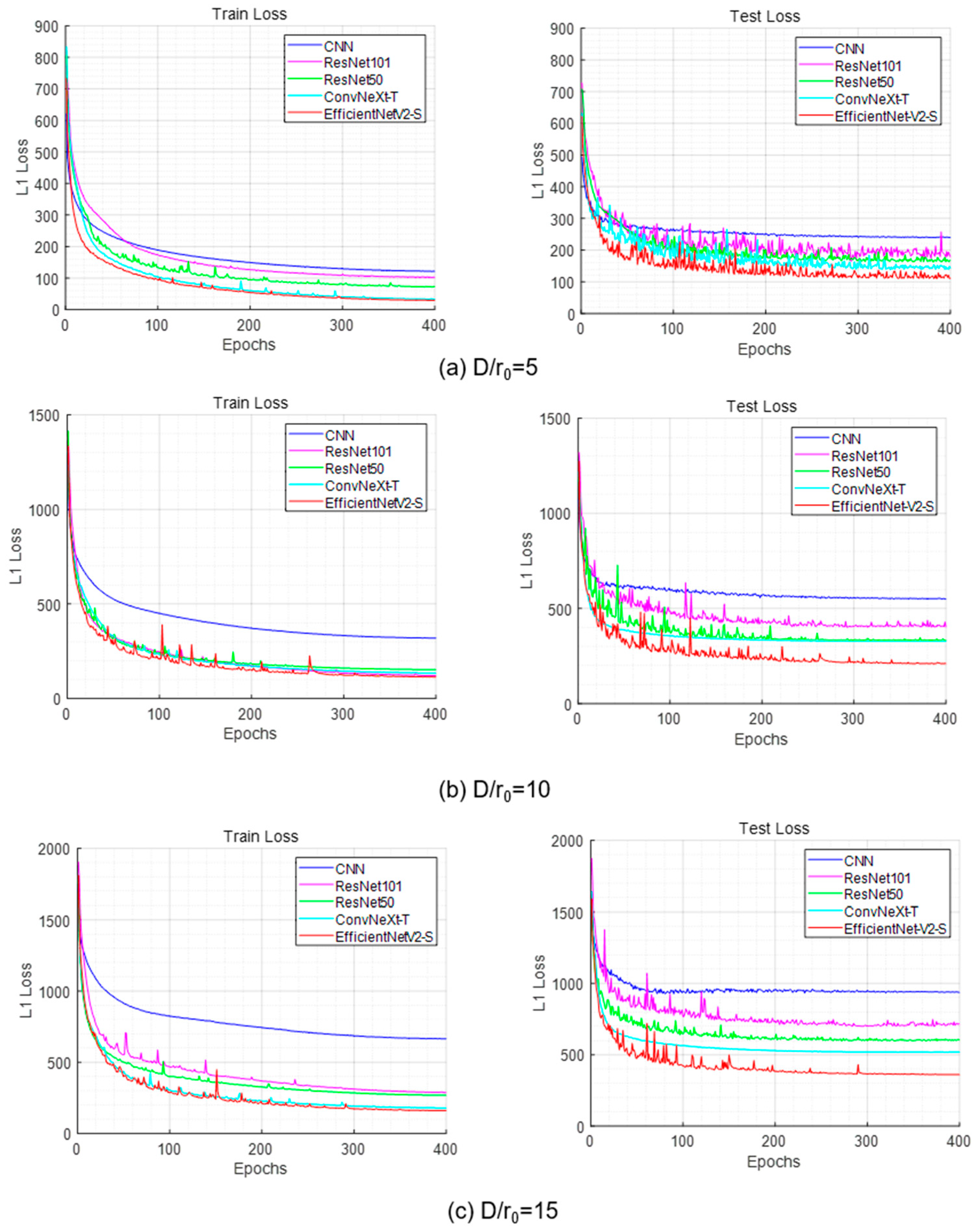
Building upon the ablation study, we further evaluated the proposed approach against several widely used deep learning models to comprehensively assess its effectiveness. We trained the conventional CNN, ResNet50, ResNet101, ConvNeXt-T, and EfficientNetV2-S using 15,000 training images and 1000 validation images. Figure 10a–c present the training and validation loss curves computed by Equation (8). For all models, the loss decreases with increasing epochs and gradually converges to a stable level. Across both weak and strong turbulence conditions in WFS-less AO, EfficientNetV2-S consistently converges faster and achieves the lowest final L1 loss, indicating its superior stability. Benefiting from the efficient feature representation of Fused-MBConv and SE modules and effective feature reuse, it maintains lower loss and more stable outputs, demonstrating stronger robustness and generalization.

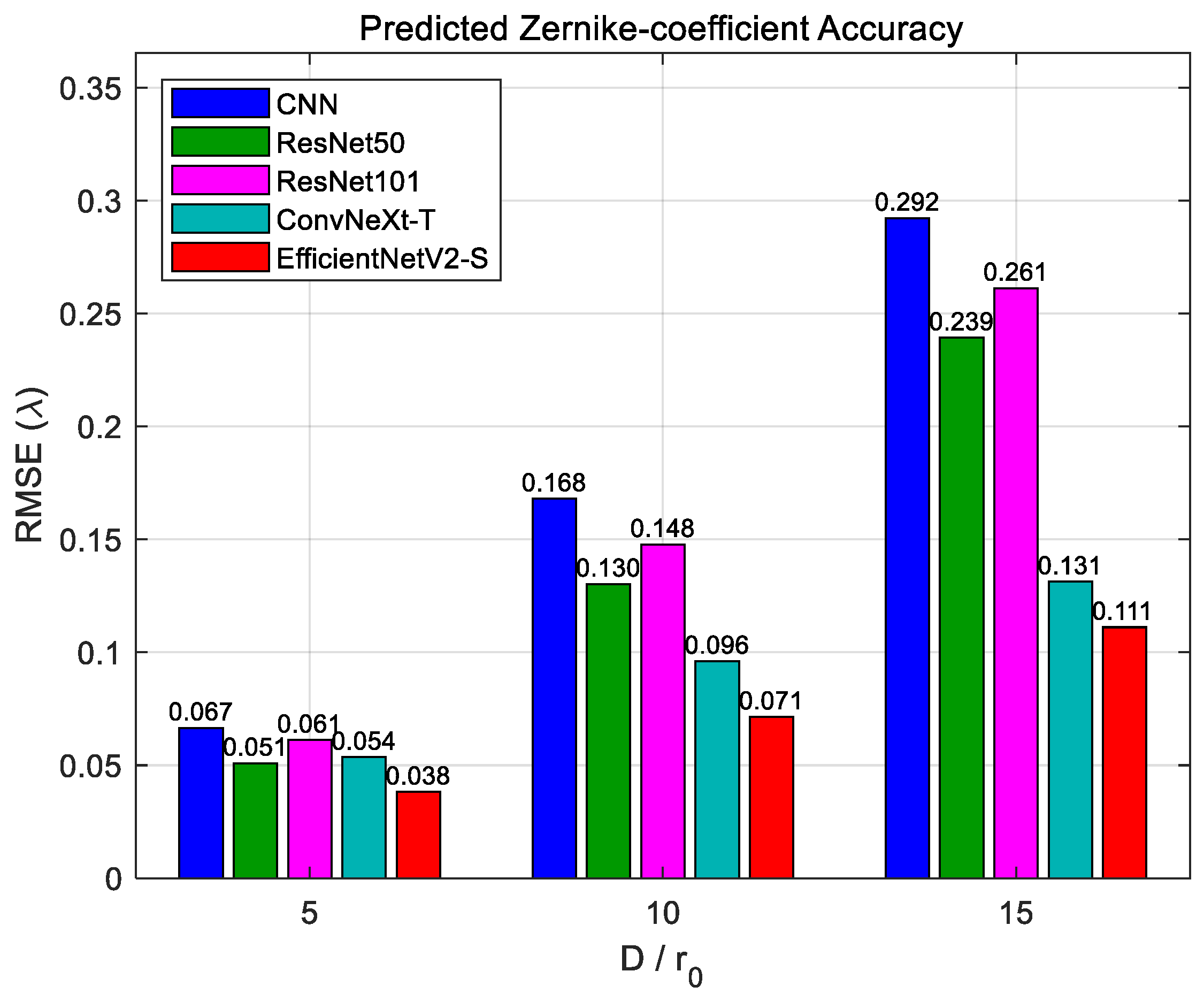
Figure 11 provides a quantitative comparison of the Zernike coefficient prediction errors (in units of λ) for the five networks under different turbulence strengths D/r₀ = 5, 10, and 15. When the atmospheric turbulence strength is specified as D/r₀ = 5, the ZRMSE of the conventional CNN, ResNet50, ResNet101, ConvNeXt-T, and EfficientNetV2-S are 0.067λ, 0.051λ, 0.061λ, 0.054λ, and 0.038λ, respectively. When D/r₀ = 10, the ZRMSE for the five respective networks are 0.168λ, 0.128λ, 0.148λ, 0.096λ, and 0.071λ. When D/r₀ = 15, the ZRMSE for the five respective networks are 0.292λ, 0.239λ, 0.261λ, 0.131λ, and 0.111λ.

As the turbulence strength increases, EfficientNetV2-S shows a more pronounced advantage over the other models. This is mainly attributed to the efficient feature extraction of Fused-MBConv, the enhanced channel representation provided by SE attention, and the well-balanced depth–width configuration enabled by compound scaling. Meanwhile, the chart indicates that ResNet50 outperforms ResNet101 in both loss value and wavefront detection accuracy. Increasing network depth introduces more nonlinear transformations, which may cause feature information to degrade and lead to “network degradation”, making training more difficult. Although residual connections can mitigate this effect, their benefit diminishes when the network becomes excessively deep, resulting in poorer training performance.

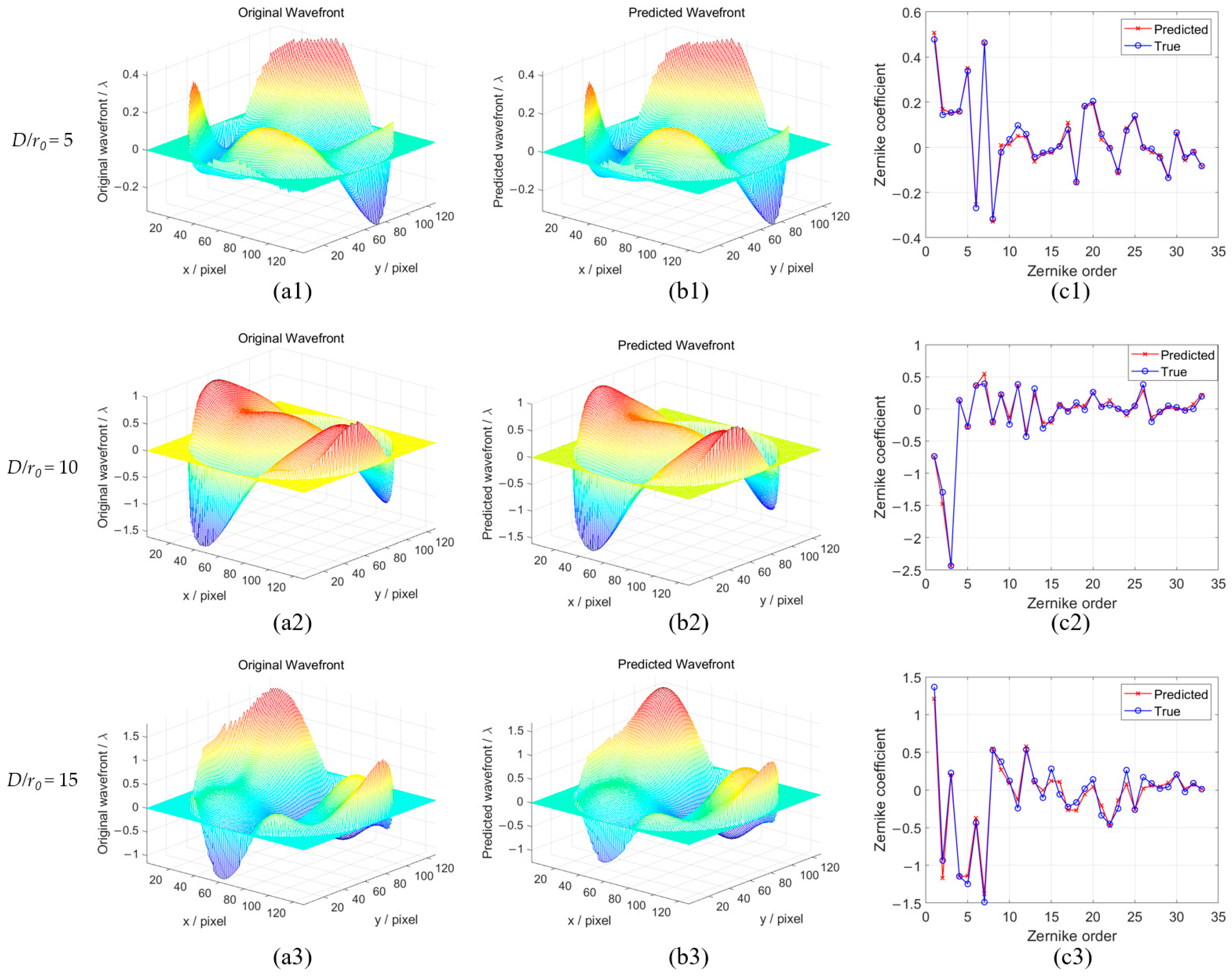
The first column shows the true wavefront, the second column shows the wavefront predicted by EfficientNetV2-S, and the third column shows the residual wavefront aberration. As shown in the figures, across different turbulence intensities, the wavefront reconstructed by EfficientNetV2-S is highly consistent with the 3D morphology of the true wavefront: peak/valley locations and high-order fluctuations are captured with good accuracy, indicating strong nonlinear fitting ability and good generalization in predicting high-order Zernike coefficients.

However, as turbulence increases, the reconstruction accuracy decreases. Under strong turbulence (D/r₀ = 15), a slight phase discontinuity ring appears near the pupil edge. With stronger turbulence, recovery errors for high-order Zernike distortion coefficients become more pronounced, which may be attributed to the limited resolution of the simulation grid and the greater complexity of recovering high-order distortions.

The evaluation of randomly selected samples at D/r₀ = 5, 10, and 15 shows that the model maintains good performance under varying turbulence strengths. As illustrated in Figure 12 (final epoch), an accurate prediction of Zernike coefficients from the 3rd to the 35th order is achieved. Even under strong turbulence, despite increased errors, the model preserves reasonable amplitude distributions and trends, offering reliable prior information for subsequent wavefront compensation.

3.2. Experimental Validation

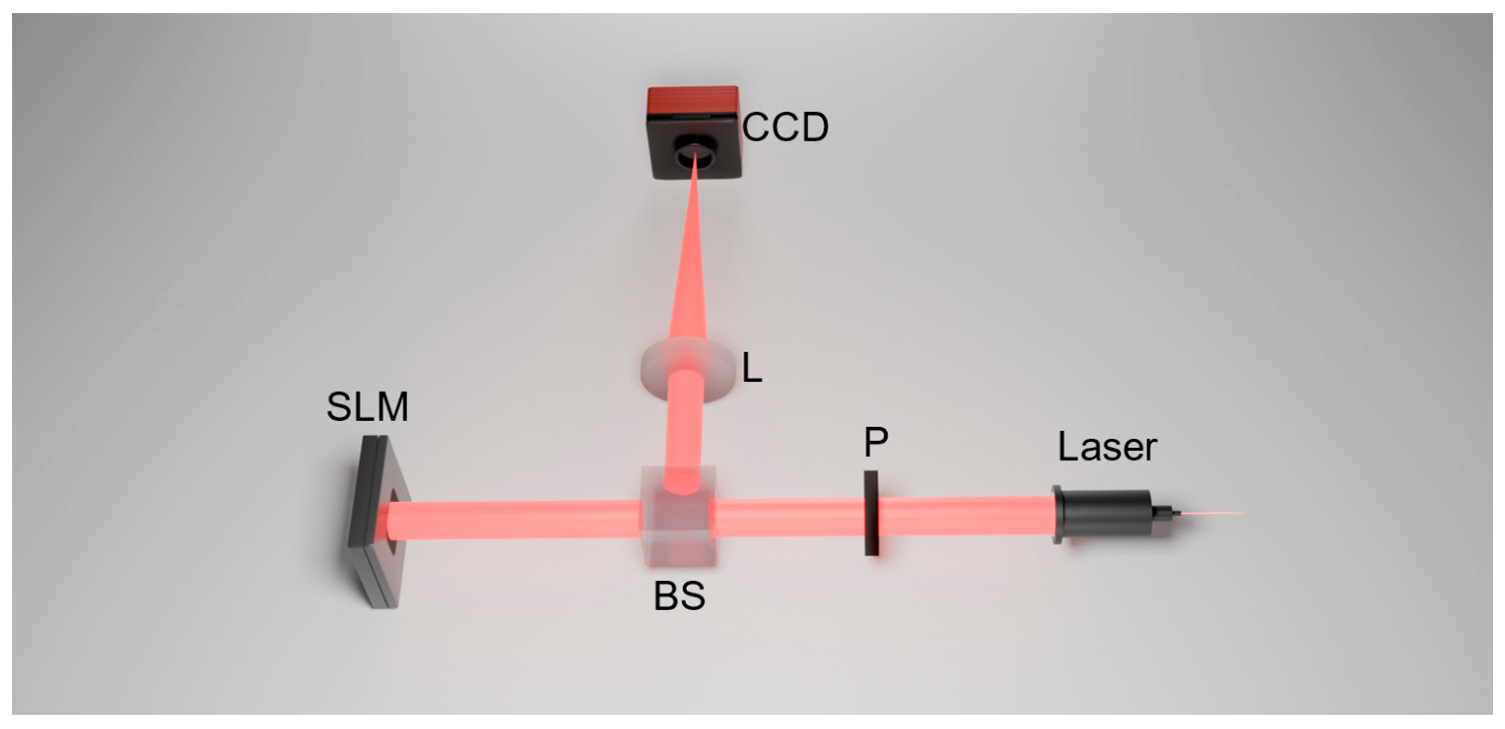
To further validate the feasibility of the proposed method, a real-world experiment has been conducted. The experimental optical setup is schematically illustrated in Figure 13. This section directly uses the data collected from the experimental system to train an EfficientNetV2-S model. It mainly consists of a light source (Laser), a linear polarizer (P), a beam splitter (BS), a spatial light modulator (SLM), a focusing lens (L), a CCD camera, and a PC. The polarizer aligns the laser’s polarization direction to meet the operational requirements of the SLM. The SLM is then used to modulate the optical path length of the beam, thereby emulating atmospheric turbulence disturbances. Key parameters of the SLM and the camera are listed in

Table 6. Specific parameters of the SLM and the camera.

Devices	Pixel Size	Number of Pixels	Bit Depth
SLM	9.2 µm × 9.2 µm	1920 × 1152	12-bit
CCD	3.45 µm × 3.45 µm	1920 × 1200	12-bit

.

The SLM employed in the experimental platform is a liquid-crystal optical phased array manufactured by Meadowlark Optics Inc. (Frederick, CO, USA). Image acquisition is performed using a Teledyne BFS-U3-23S3C-C camera (Thousand Oaks, CA, USA). All experiments are conducted within a PyTorch-based deep learning framework on a computing platform running Windows 11. The hardware configuration includes an Intel Core i9-10900K CPU operating at 3.7 GHz, 32 GB of DDR4 memory, and an NVIDIA GeForce RTX 2080 Ti GPU. To simulate wavefront perturbations induced by atmospheric turbulence, Zernike mode coefficients following a Kolmogorov turbulence spectrum are first randomly generated. Based on these coefficients, grayscale images are synthesized under different turbulence strengths, specifically D/r₀ = 5 and 10.

The synthesized grayscale images were sequentially loaded onto the SLM to generate the corresponding disturbed wavefronts. During this process, the coefficients of the first two Zernike modes (piston and tip–tilt) were set to zero. The camera was positioned at the focal plane of the lens to acquire focal-plane images. Rather than physically translating the camera to obtain defocused-plane images, a defocus aberration with a peak-to-valley (PV) value of one wavelength was introduced by applying an additional phase term to the SLM. In total, 13,000 data samples were collected. Each sample consists of one focal-plane image, one defocused-plane image, and the corresponding Zernike coefficients from the 3rd to the 35th order describing the disturbed wavefront. The complete dataset was divided into a training set and a test set containing 12,000 and 1000 samples, respectively.

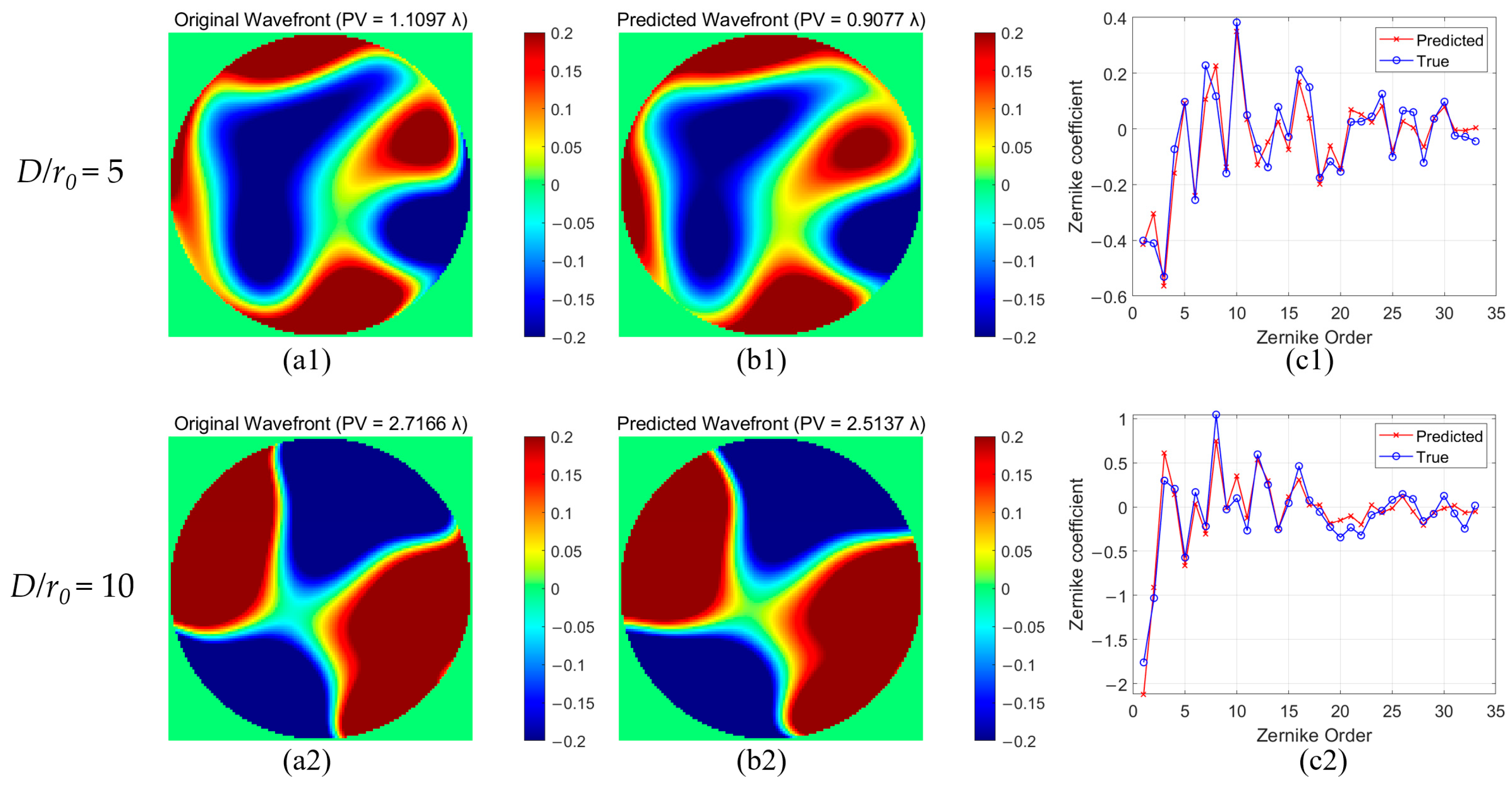
The wavefront reconstruction results of the EfficientNetV2-S network under the conditions of D/r₀ = 5 and D/r₀ = 10 are shown in Figure 14. For D/r₀ = 5, the PV values of the initial and predicted wavefronts are 1.1097λ and 0.9077λ, respectively. The model successfully recovers the overall wavefront morphology, and the predicted 3rd to 35th-order Zernike coefficients are highly consistent with the ground truth. Although the recovery error for higher-order aberrations is relatively larger, especially near the pupil boundary, the model still effectively reconstructs the wavefront morphology.

When D/r₀ = 10, the PV values of the initial and predicted wavefronts are 2.7166λ and 2.5137λ, respectively. As the turbulence intensity increases, the wavefront reconstruction performance exhibits a slight degradation; however, the model remains capable of recovering wavefronts with similar spatial morphology. These results demonstrate that EfficientNetV2-S can provide reliable and effective prior information across varying turbulence conditions, thereby facilitating subsequent wavefront compensation.

4. Conclusions

This paper presented a deep learning-based wavefront prediction framework for WFS-less AO using EfficientNetV2-S as the backbone network. By leveraging focused–defocused image pairs and directly regressing Zernike coefficients in a single forward pass, the proposed method avoids iterative optimization and effectively addresses the ambiguity inherent in single-intensity measurements. The framework enables the efficient and accurate prediction of high-order wavefront aberrations under various turbulence conditions. Comprehensive simulation and experimental results demonstrate that EfficientNetV2-S consistently outperforms conventional CNNs as well as representative modern architectures, including ResNet50/101 and ConvNeXt-T, in terms of L1 loss and ZRMSE. Ablation studies further confirm that key architectural components—namely the Fused-MBConv blocks and the SE attention mechanism—play a critical role in improving feature extraction, training stability, and robustness, particularly under medium-to-strong turbulence where high-order aberrations dominate. Even as turbulence intensity increases and overall prediction errors rise, the proposed model remains capable of recovering wavefronts with reasonable spatial morphology, providing reliable prior information for subsequent wavefront compensation. Beyond prediction accuracy, EfficientNetV2-S offers a favorable balance between representational capability and computational efficiency. Its compact parameter size and low inference latency make it well suited for real-time wavefront prediction, which is essential for practical WFS-less AO systems. These characteristics are particularly advantageous for deployment on embedded and edge-computing platforms, such as NVIDIA Jetson devices, where computational resources and power budgets are limited.