Frequency Modulation Spectroscopy and Modulation Transfer Spectroscopy for Laser Stabilization to Rubidium Atomic Resonances

Abstract

We make a detailed comparison of frequency modulation spectroscopy (FMS) and modulation transfer spectroscopy (MTS) and of their applications in stabilizing laser frequency. In both FMS and MTS, intensity modulations of probe beam are observed in saturated absorption spectroscopy of ⁸⁷Rb atoms. However, the two modulation profiles appear different due to their distinct origins. Demodulation gives rise to frequency discrimination spectra, which can serve as error signals for frequency locking. The optimal error signal of FMS has a larger linear slope but also a slanted baseline, in contrast to that of MTS. We apply FMS and MTS to stabilize two 780 nm external cavity diode lasers to $D_2$ lines of ⁸⁷Rb atoms. We measure laser linewidth and stability using beat notes of two independently locked lasers. A laser linewidth as narrow as 12.9 kHz is achieved in FMS locking, compared to 70.8 kHz in MTS locking. A laser stability at the level of 10⁻¹² is reached in both schemes. Nevertheless, FMS locking offers a better short-term stability, whereas MTS locking yields a smaller long-term drift. Our investigation of FMS and MTS would be valuable for making a choice of these spectroscopy techniques for laser stabilization as well as other relevant applications.

1. Introduction

Lasers have been utilized for manipulating and detecting states of atoms, molecules, and other microscopic particles or even macroscopic objects for various kinds of quantum technologies, including time and frequency standards [1], precision sensing [2,3], quantum computation [4,5], and many others. It is absolutely necessary to stabilize the laser frequency in these applications to achieve minimal drifts and narrow instantaneous linewidth, so that coherence of the laser field is maintained as much and as long as possible for efficient and precise control of quantum states. Among a plethora of stabilization techniques [6], those involving interferometric modulation are widely used [7,8,9,10,11]. Such schemes have some vary desirable features. For one, zero crossings of the error signal reside at spectral resonances and are not much affected by the fluctuation of laser intensity and polarization or other environmental factors. For another, modulation frequencies are often in the range of MHz or higher and quite away from low frequency noises. These modulation-based locking schemes have many variations, especially with regard to locking references. The Pound–Drever–Hall (PDH) scheme typically refers to locking laser frequency to optical cavity modes [12]. Frequency modulation spectroscopy (FMS) employs a similar modulation technique but uses atomic resonances as references [13]. Moreover, optical frequency/phase lock loop (OFLL/OPLL) utilizes a stabilized laser system or an optical frequency comb as references, where beat notes between the reference laser and the laser to be locked are demodulated to generate an error signal for locking [14].

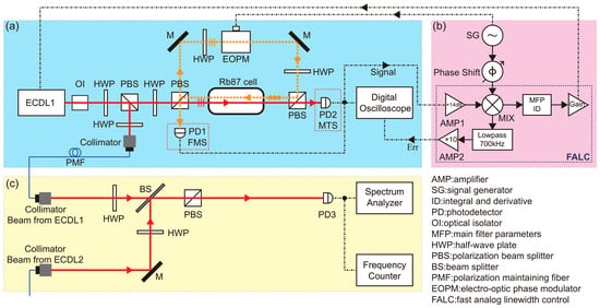
Closely related to FMS is modulation transfer spectroscopy (MTS). The setups for both FMS and MTS are based on saturated absorption spectroscopy (SAS) of atomic transitions and appear nearly the same, other than the position of photo detector (PD), as indicated in Figure 1a. In a SAS setup, the laser beam going into PD is defined to be the probe and the other beam counter-propagating in the atomic vapor cell to be the pump. In the case of FMS, it is the probe that goes through an electro-opto phase modulator (EOPM), and in the case of MTS, it is the pump. Accordingly, the modulation of the probe beam in FMS directly comes from EOPM, but that in MTS is transferred from the modulation of the pump beam via a nonlinear four-wave mixing process. Both FMS and MTS can be used for laser locking, where frequency discrimination spectroscopy (FDS) is generated after demodulating the PD signal and serves as error signals to be fed back to the laser, as sketched in Figure 1b. The distinct modulation origins of FMS and MTS give rise to the modulation profiles of different shapes and consequently, and the resulting error signals of FMS and MTS offer different advantages in laser stabilization. FMS had already become an important locking technique in the 1980s [8,9,13], while initial work on FMS started much earlier [15]. MTS was applied to locking at a later time than FMS [16], even though MTS spectroscopic study started in the early 1980s [10,17,18,19,20]. MTS locking has gathered more attention in recent years [11,21,22,23,24,25,26,27], and there are even works combining FMS and MTS in order to achieve better locking [28].

Figure 1. Schematics of experimental setup. (a) Optical setup. A SAS setup mainly consists of two laser beams overlapping and counter-propagating through the atomic vapor cell. In the figure, the two lines representing two overlapping beams inside the cell are purposely displaced for the sake of clarity. An EOPM is placed in one beam path to introduce modulation before the beam enters the vapor cell. Depending on a PD’s position, PD1 (PD2) detects FMS (MTS) signals, which are then observed in a digital oscilloscope and sent to locking electronics. (b) Locking electronics. Inside a commercially available FALC, spectroscopic signals are demodulated to produce error signals, which are monitored by a digital oscilloscope. After going through a PID controller and an amplifier, error signals are then fed back to the laser in (a) for frequency stabilization. (c) Beat measurement setup. Beat notes are produced from the locked ECDL in (a) and another ECDL of similar specifications that is locked with the same spectroscopic technique. Beat notes are then measured by a spectral analyzer and a frequency counter, and the measurement results are analyzed to derive the linewidth and stability of two locked lasers. The model numbers of the instruments used in our experiment are listed in Table S1 of the Supplementary Materials.

Notwithstanding the extensive adoption of MTS and FMS in laser frequency stabilization, the existing literature exhibits notable deficiencies. First, the limited experimental comparisons reported to date have generally been conducted on distinct setups or under disparate conditions, thereby precluding a clear understanding of the intrinsic differences between the two locking schemes and their respective advantages. Second, the modulation frequency, which critically affects both the error-signal shape and the locking performance, has not been investigated for MTS and FMS across a wide frequency range. Third, despite the availability of independent theoretical treatments for each method, a unified simulation framework enabling direct comparison of their modulation profiles under identical conditions has yet to be established. This work provides a combined experimental and theoretical comparison of MTS and FMS under identical conditions.

In this paper, we conduct a detailed comparison of FMS and MTS spectroscopy before and after demodulation as well as their applications in locking laser frequency. We observe the probe intensity modulations of FMS and MTS in SAS, which clearly reveal different profiles near sub-Doppler resonances. We compare these modulation profiles with their respective analytical formulas and find good agreements. Frequency discrimination spectroscopy is obtained by demodulating the PD signals of FMS and MTS, which has a linear slope at each resonant peak where modulation is present. Such a frequency discrimination signal is well suited to serve as an error signal for laser locking. We characterize the optimal error signal slopes from FMS and MTS at different modulation frequencies in order to find the best locking parameters. FMS and MTS are then used to stabilize the frequencies of two external cavity diode lasers (ECDLs), which are locked independently, either via FMS or via MTS. The locking performance is evaluated with beat notes between two lasers. We measure laser linewidths achieved when locking via FMS or MTS at four modulation frequencies. The laser linewidths and the error signal slopes are inversely correlated. As the error signals of FMS have considerably larger slopes than that of MTS, FMS locking results in a narrower instantaneous linewidth. From the fractional Allan variance, it is evaluated that lasers locked via MTS appear to have a better long-term stability, due to the flat baseline of its error signal. The systematic measurements and comparisons presented in the paper should be useful when making choices in using either FMS and MTS in a variety of laser stabilization applications.

2. Spectroscopy Principles and Measurements

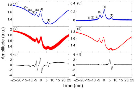
FMS and MTS are typically observed in atomic vapor cells at room temperature or at some elevated temperatures. At these conditions, Doppler broadening can reach ∼ GHz and a sub-Doppler spectral technique, such as SAS, is necessary to resolve transitions between hyperfine atomic levels. A SAS setup with a room-temperature cell of enriched ⁸⁷Rb vapor is shown in Figure 1a. A probe beam and a pump beam, both derived from a 780 nm ECDL of frequency ${\nu }_c$, overlap and counter-propagate inside the atomic vapor cell. As ${\nu }_c$ scans through D2 transitions $|5S_{1/2},F=2⟩\to |5P_{3/2},F^{\prime }=1,2,3⟩$, SAS can be detected by PD and observed on an oscilloscope. When no EOPM is present or turned on in the optical path, the SAS detected by either of the two PDs in Figure 1a is nearly identical to each other. A typical SAS is shown in Figure 2a, which contains six sub-Doppler spectral peaks sitting on the Doppler-broadened absorption profile. The plot in Figure 2b is a difference spectrum of subtracting the Doppler-broadened absorption from SAS. We regard each of the sub-Doppler spectral peaks in Figure 2b as a generic atomic resonance of the Lorentzian profile with a central frequency ${\nu }_0$ and a full width at half maximum (FWHM) of $\Delta \nu$,

$$g\left(\nu \right)={\displaystyle \frac{\Delta \nu /2\pi }{{(\nu -{\nu }_0)}^2+{(\Delta \nu /2)}^2}}.$$

(1)

Figure 2. (a) SAS of the ⁸⁷Rb D2 transitions $|5S_{1/2},F=2⟩\to |5P_{3/2},F^{\prime }=1,2,3⟩$. (b) Difference between SAS and the Doppler broadened absorption of the probe itself with no pump beam present. The sub-Doppler spectral peaks in (a,b) are labeled to be (1)–(6), where (1)–(3) represent the transitions $|5S_{1/2},F=2⟩\to |5P_{3/2},F^{\prime }=3,2,1⟩$ respectively, and (4)–(6) correspond to the crossovers between the transitions (1) and (2), between the transitions (1) and (3), and between the transitions (2) and (3). (c) Modulated SAS in FMS, where EOPM is placed in the probe beam path. (d) Modulated SAS in MTS, where EOPM is placed in the pump beam path. In both (c,d), the EOPM is driven with modulation frequency ${\nu }_m$ = 25 MHz. FDS after demodulation and filtering of FMS (e) and of MTS (f). All spectra (a–f) are obtained by scanning the laser carrier frequency ${\nu }_c\left(t\right)=v_{f}t+{\nu }_d$ with the same $v_f$ = 20.85 GHz/s and the same ${\nu }_d$ and observed on a digital oscilloscope. The position and the HWHM of the sub-Doppler peak (i), $t_i$ and $t_{{\Gamma }_i}$ with $i\in \{1,4,5\}$, are obtained by fitting the multiple resonances in (b) with the Lorentizian lineshape. Moreover, the scanning speed $v_f$ is derived from $|t_1-t_4|$. The offset frequency ${\nu }_d$ is set such that $t_4\sim 0$ on the digital oscilloscope.

2.1. Frequency Modulation Spectroscopy

When an EOPM driven with frequency ${\nu }_m$ is placed in the optical path as illustrated in Figure 1a, the laser beam of frequency ${\nu }_c$ passing through EOPM obtains frequency sidebands ${\nu }_c\pm n{\nu }_m$, whose amplitudes are given by Bessel functions $J_n$

$$\begin{array}{cc}\hfill E_L\left(t\right)& =E_0\sin ({\omega }_{c}t+M\sin {\omega }_{m}t)\hfill \\ \hfill & =E_0\left[{\displaystyle \sum _{n=0}^{\infty }}{J}_n\left(M\right)\sin ({\omega }_c+n{\omega }_m)t+{\displaystyle \sum _{n=1}^{\infty }}{(-1)}^n{J}_n\left(M\right)\sin ({\omega }_c-n{\omega }_m)t\right]\hfill \end{array},$$

(2)

where ${\omega }_{c,m}=2\pi {\nu }_{c,m}$, and M is the modulation index. The modulation index is generally small and higher-order sidebands of $n>1$ are usually negligible. If only the first-order sidebands of ${\nu }_c\pm {\nu }_m$ are included, the modulated laser field can be simplified as

$$E_L\left(t\right)=E_0\left[J_0\left(M\right)\sin {\omega }_{c}t+J_1\left(M\right)\sin ({\omega }_c+{\omega }_m)t-J_1\left(M\right)\sin ({\omega }_c-{\omega }_m)t\right].$$

(3)

When this frequency modulated laser beam passes through an atomic gas near a resonance ${\nu }_c\sim {\nu }_0$, the sidebands and the carrier see different complex transmission coefficients $T\left(\nu \right)=\exp (-\delta (\nu )+i\varphi (\nu \left)\right)$ at their respective frequencies, where the real and imaginary components of T specify absorption and phase shift from dispersion, respectively. Interference of three frequency components (${\nu }_c,{\nu }_c\pm {\nu }_m$) results in intensity modulation. When the laser frequency ${\nu }_c$ is far away from atomic resonances, all three frequencies see the same transmission $T\left({\nu }_c\right)=T({\nu }_c\pm {\nu }_m)$. When ${\nu }_c$ is exactly at an atomic resonance ${\nu }_c={\nu }_0$, the transmissions of the two sidebands are the same $T({\nu }_c+{\nu }_m)=T({\nu }_c-{\nu }_m)$, but different from $T\left({\nu }_c\right)$. In either of the two latter cases, interference of frequency components is canceled out with no resulting intensity modulation.

For FMS, the EOPM is placed in the optical path of the probe and the modulated probe counter-propagates against the unmodulated pump inside the atomic vapor cell and is then detected by a PD, as illustrated in Figure 1a. The intensity modulation in FMS near a sub-Doppler SAS resonance, due to the three frequency components in Equation (3), is expressed by [7,10]

$$\begin{array}{cc}\hfill S_{\mathrm{FMS}}\left({\omega }_m\right)& =C{J}_0\left(M\right)J_1\left(M\right)\times \left[(L_{1/2}-L_{-1/2})\cos \left({\omega }_{m}t\right)+(D_{1/2}+D_{-1/2}-2D_0)\sin \left({\omega }_{m}t\right)\right]\hfill \\ \hfill & =C{J}_0\left(M\right)J_1\left(M\right)\times \left[L_{\mathrm{FMS}}\left({\omega }_m\right)\cos \left({\omega }_{m}t\right)+D_{\mathrm{FMS}}\left({\omega }_m\right)\sin \left({\omega }_{m}t\right)\right]\hfill \end{array}.$$

(4)

In the above Equation (4), $L_{n/2}$ and $D_{n/2}$, where n = 0 & ±1, are the absorption and dispersion functions associated with the generic Lorentzian resonance of Equation (1) [9,10],

$$L_{n/2}={\displaystyle \frac{{\Gamma }^2}{{\Gamma }^2+{({\omega }_c-{\omega }_0+(n/2){\omega }_m)}^2}},D_{n/2}={\displaystyle \frac{\Gamma \times ({\omega }_c-{\omega }_0+(n/2){\omega }_m)}{{\Gamma }^2+{({\omega }_c-{\omega }_0+(n/2){\omega }_m)}^2}},$$

(5)

where ${\omega }_0=2\pi {\nu }_0$ and $\Gamma =2\pi (\Delta \nu /2)$ are the angular frequencies of the spectral peak and of half width at half maximum (HWHM). Moreover, the constant C in Equation (4) characterizes the properties of the atomic gas and the probe and pump beams other than those specified in the above equations.

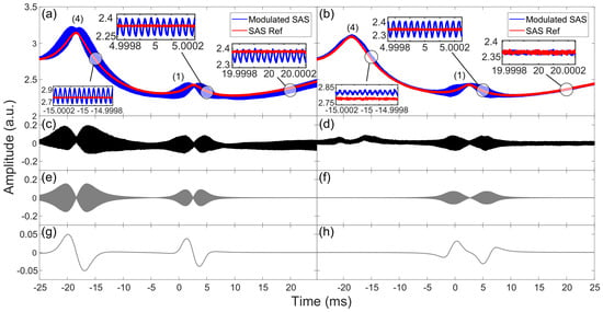
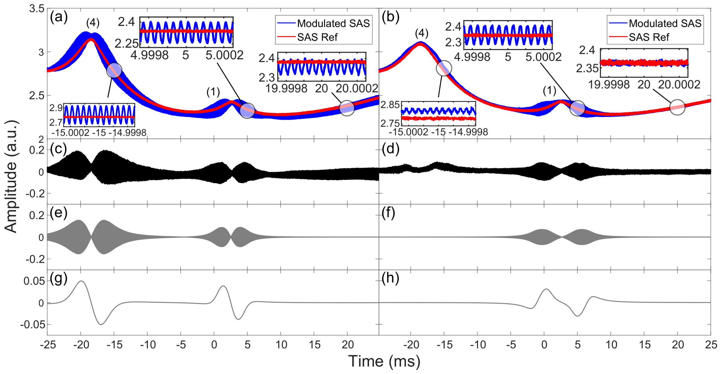
The modulated SAS in FMS is shown in Figure 2c, where the spectral line is obviously thicker than in Figure 2a due to intensity modulation, which is however unresolved at this scale. Note that intensity modulation in FMS appears not only near the sub-Doppler resonances but also across the whole range of the Doppler-broadened absorption profile. The reason is that the origin of modulation, as explained in the paragraph following Equation (3), also applies to the Doppler-broadened absorption resonance. This is in contrast to the case of MTS, as detailed in Section 2.2. A zoomed view of SAS in Figure 2a and the modulated SAS in Figure 2c is shown in Figure 3a, where some detailed features become visible. Due to the interference cancellation, the amplitude of intensity modulation is near zero at the resonant peaks (1) and (4). From the further zoomed spectral segments given in the three inset figures, the intensity modulation of frequency ${\nu }_m$ = 25 MHz is clearly seen. Figure 3c is the difference of the two plots in Figure 3a, where the amplitude variation of the intensity modulation can be described by Equation (4). To simulate the FMS modulation signal in Figure 3c, we first transform the absorption and dispersion functions of frequency in Equation (5) into the corresponding functions of time,

$$L_{n/2}={\displaystyle \frac{t_{{\Gamma }_i}^2}{t_{{\Gamma }_i}^2+{(t-t_i+(n/2)({\nu }_m/v_f))}^2}},D_{n/2}={\displaystyle \frac{t_{{\Gamma }_i}(t-t_i+(n/2)({\nu }_m/v_f))}{t_{{\Gamma }_i}^2+{(t-t_i+(n/2)({\nu }_m/v_f))}^2}},$$

(6)

where the values of $t_i$ and $t_{{\Gamma }_i}$ ($i\in \{1,4\}$) as well as $v_f$ are specific to Figure 3. By inserting Equation (6) into Equation (4) and leaving C as a free parameter, we plot in Figure 3e the FMS signals around peaks (1) and (4). The calculated modulation profile of Figure 3e agrees well with the experimental profile shown in Figure 3c. Note that the residual modulations on the base line of Figure 3c are due to the Doppler-broadened absorption and not included in the simulation described above.

Figure 3. Zoom-in view of SAS and modulated SAS of FMS (a) and of MTS (b), where only the two strongest sub-Doppler resonances (1) and (4) are included. The modulation frequency ${\nu }_m$ = 25 MHz and the scanning speed $v_f$ = 6.35 GHz/s, which is calculated in the same way as that described in the caption of Figure 2. For a direct comparison, a slight offset has been added so that SAS and the modulated SAS are overlapped at the resonance peak (1). Three different segments on the modulated SAS of FMS (MTS) are displayed in the three inset figures of (a) (of (b)), where the presence of intensity modulation (${\nu }_m$ = 25 MHz) are clearly seen. Difference between SAS and the modulated SAS of FMS (c) and of MTS (d). The differences are obtained by subtracting SAS from the modulated SAS in (a) and (b) respectively. Simulated intensity modulation using Equation (4) for FMS (e) and using Equation (7) for MTS (f), together with Equation (6). Simulated FDS using Equation (8) for FMS (g) and for MTS (h).

2.2. Modulation Transfer Spectroscopy

For MTS, an EOPM is placed in the optical path of the pump, not of the probe as in FMS. In contrast to FMS, the probe is unmodulated before entering the atomic vapor cell. However, since the probe counter-propagates against the modulated pump inside the atomic vapor cell, the modulation of the pump beam can be transferred via a nonlinear four-wave mixing process to the probe, which is then detected by a PD as depicted in Figure 1a. An efficient four-wave mixing process requires energy conservation and phase matching, and within the atomic medium, these conditions are best fulfilled near the cycling transition $|5S_{1/2},F=2⟩\to |5P_{3/2},F^{\prime }=3⟩$, that is, near the peak (1) of SAS. The atoms that see this transition have nearly zero velocity along the propagation of the beams and are driven by the pump and the probe at a closed cycle with a minimal population leakage to other levels. Four-wave mixing then results in two new frequency components ${\nu }_c\pm {\nu }_m$ co-propagating with the probe beam of frequency ${\nu }_c$. As seen in Figure 2d, intensity modulations appear much stronger near peak (1) than other resonances. The MTS modulation, when only counting the first-order sidebands, is expressed by [10,11]

$$\begin{array}{cc}\hfill S_{\mathrm{MTS}}\left({\omega }_m\right)& =C^{\prime }{J}_0\left(M\right)J_1\left(M\right)\times \left[(L_{-1}-L_{-1/2}+L_{1/2}-L_1)\cos \left({\omega }_{m}t\right)+(D_1-D_{1/2}-D_{-1/2}+D_{-1})\sin \left({\omega }_{m}t\right)\right]\hfill \\ \hfill & =C^{\prime }{J}_0\left(M\right)J_1\left(M\right)\times \left[L_{\mathrm{MTS}}\left({\omega }_m\right)\cos \left({\omega }_{m}t\right)+D_{\mathrm{MTS}}\left({\omega }_m\right)\sin \left({\omega }_{m}t\right)\right]\hfill \end{array},$$

(7)

where $L_{n/2}$ and $D_{n/2}$ with n = ±1 & ±2 are the same as defined in Equation (5), and the constant $C^{\prime }$ characterizes the properties of the nonlinear process not explicitly specified in the above equation. Shown in Figure 3b is a zoomed view of SAS and the modulated SAS in Figure 2a,d, together with three further zoomed spectral segments in the inset figures. It is very clearly seen that the intensity modulation of ${\nu }_m$ = 25 MHz appears quite strong near peak (1), but only minimal near peak (4) and not obvious at all along the Doppler broadened absorption profile, which is contrary to that seen in FMS. The difference between SAS and the modulated SAS is shown in Figure 3d, which is the MTS signal described by Equation (7). The plot in Figure 3f is the simulated MTS signal produced by inserting Equation (6) into Equation (7), where the values of $t_{{\Gamma }_1}$ and $t_1$ are the same as those used to generate Figure 3e and $C^{\prime }$ is a free parameter. The calculated modulation profile of Figure 3f agrees well with the experimental profile shown in Figure 3d.

2.3. Frequency Discrimination Spectroscopy

Frequency discrimination spectroscopy can be generated when the modulated SAS in Figure 2c or in Figure 2d is sent to the electronic setup in Figure 1b, where it is amplified and mixed with the local RF oscillator that drives the EOPM. The resulting FDS from FMS is shown in Figure 2e and from MTS in Figure 2f, respectively. FDS has a frequency discrimination slope at each resonance where intensity modulations are present and this slope produced by demodulation can be expressed as

$$\begin{array}{cc}\hfill {\mathrm{FDS}}_X\left({\omega }_m\right)& ={[A\times S_{\mathrm{X}}\sin ({\omega }_{m}t+\varphi )]}_{\mathrm{lowpass} \mathrm{filter}}\hfill \\ \hfill & =A^{\prime }\times \left[L_{\mathrm{X}}\left({\omega }_m\right)\sin \left(\varphi \right)+D_{\mathrm{X}}\left({\omega }_m\right)\cos \left(\varphi \right)\right],\hfill \end{array}$$

(8)

where $A^{\prime }$ is a constant including the amplification coefficient A, and X $\in${FMS,MTS}. Shown in Figure 3g,h are the simulated FDS using Equation (8) together with the parameters of Figure 3e,f. The shape and steepness of the FDS slopes are related to the intensity modulation profiles, as expected from Equation (8). A frequency discrimination slope can be used as an error signal for laser locking. As discussed above, substantial intensity modulations appear around all six sub-Doppler peaks in FMS but only around the cycling transition peak (1) in MTS. Consequently, in FMS, FDS slopes can be clearly seen at all six sub-Doppler resonances, three of which have an adequate amplitude to be used for locking. In contrast, a FDS slope of sizable amplitude appears only at peak (1) in MTS. In the FDS from FMS, the baseline is non-flat due to the intensity modulation of the Doppler broadened absorption resonance, whereas the FDS of MTS has a very flat baseline. These FDS features offer different advantages when used as error signals for laser frequency locking applications. On the one hand, locking on the steep FDS slopes of FMS gives rise to narrow instantaneous laser linewidths; but the nearby locations and slanted baseline may cause the frequency locking points to jump between slopes or drift with the baseline. On the other hand, the FDS of MTS has a distinct single slope on a very flat background, which makes frequency locking to have a good long-term stability. In the following Section 3, we present detailed studies on using the FDS slopes of FMS and of MTS at different modulation frequencies as error signals for laser frequency stabilization.

3. Laser Frequency Stabilization

As discussed above, the FDS slopes can be used as error signals for laser frequency locking. As depicted in Figure 1b, such error signals, after processing by the PID and gain modules, are fed back to laser controllers to lock the frequency to a particular resonant peak. In the case of FMS, where several error signal slopes are available, it is more often to choose the strongest signal with the largest slope at the resonant peak (4) for locking. In the case of MTS, only the slope at the resonant peak (1) is sizable and it is the choice of locking point. In this section, we apply FMS and MTS for laser locking at four different modulation frequencies and characterize the linewidth and stability of lasers by measuring beat notes of two independently locked lasers.

3.1. Error Signals

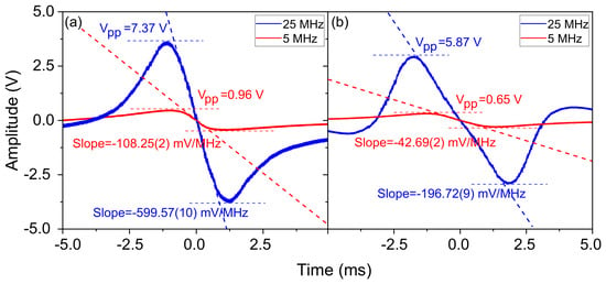
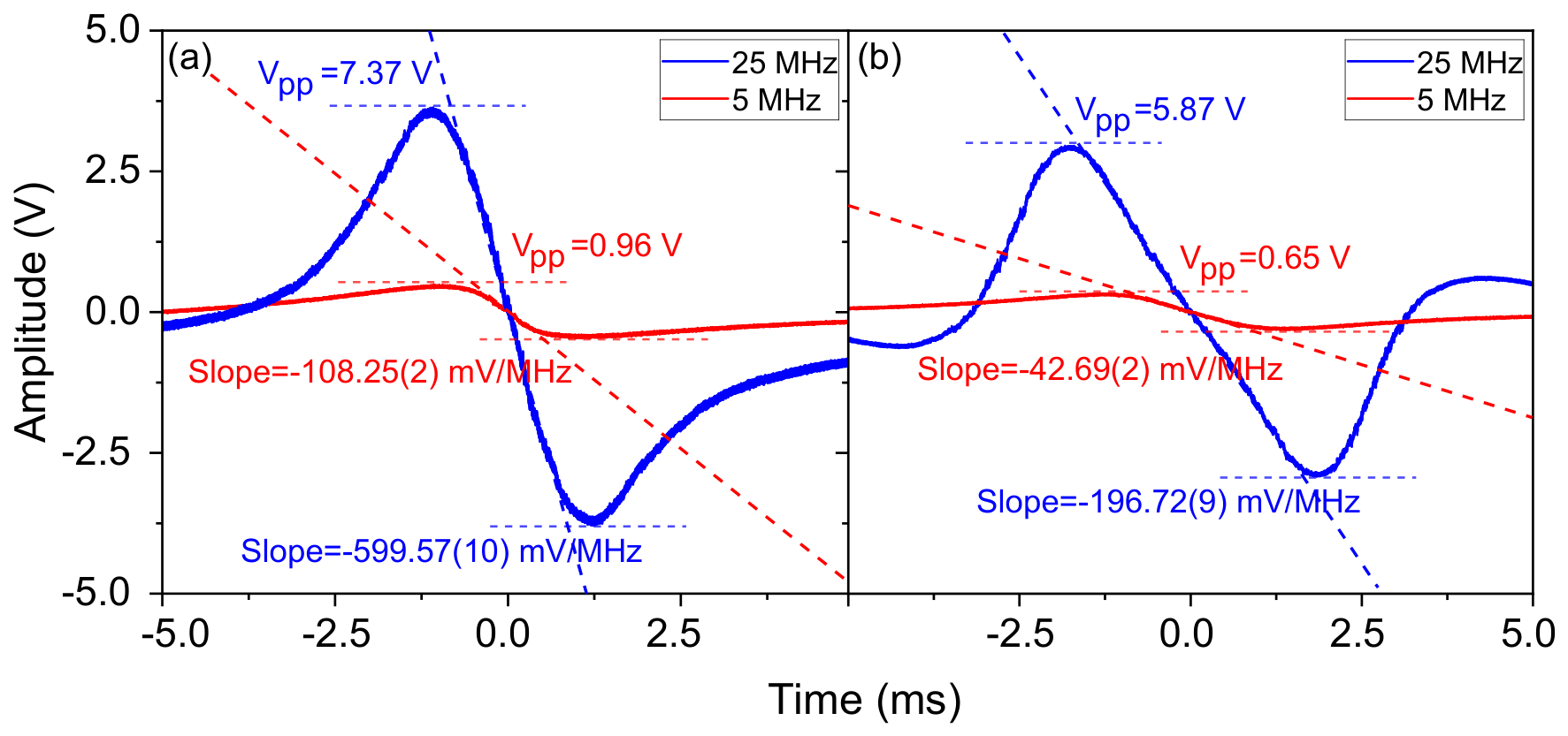
Shown in Figure 4a,b are the error signals of FMS and of MTS with ${\nu }_m$ = 5 MHz and 25 MHz, respectively. These error signals have been optimized for maximal amplitudes. Detailed system operating parameters and procedures can be found in the Supplementary Materials.

Figure 4. Error signals of FMS at ${\nu }_m$ = 5 MHz and at ${\nu }_m$ = 25 MHz (a) and of MTS at ${\nu }_m$ = 5 MHz and at ${\nu }_m$ = 25 MHz (b). In this figure, the scanning speed $v_f$ = 8.23 GHz/s. The slopes are acquired with linear fitting and the uncertainties come from fitting error. It should be noted that the experimental error signals presented in this figure were acquired after filtering, amplification and some other electronic processing within the FALC. Meanwhile, the simulated error signals in Figure 3g,h have the application factor set to be 1.

The linear slopes of such error spectra near resonances can be extracted by linear fit, as illustrated in Figure 4a,b. It can be seen that the error signal slopes of FMS are considerably larger than that of MTS. This can be understood by examining the modulation profiles shown in Figure 3c,d and the theoretical plots in Figure 3e–h. One reason is that the modulation amplitude of peak (4) used as the locking point in FMS is substantially larger than that of peak (1) used as the locking point in MTS. Another is that the two modulation maxima at the two sides of a resonance are closer to each other in FMS than in MTS. A larger slope of error signal is generally more desirable as it results in a larger feedback when the laser frequency deviates from the locking point, hence in a stronger locking. Note that the direct comparison of error signal slopes is justified by similar experimental conditions.

3.2. Laser Linewidths

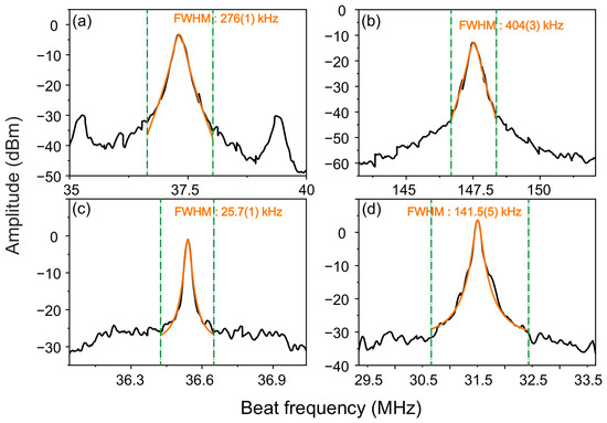
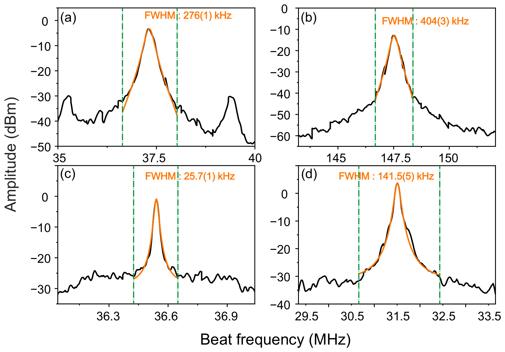
To characterize laser linewidths, we perform beat measurements between two ECDLs independently locked via either FMS or MTS. The beat measurement setup is shown in Figure 1c, where the other laser is not pictured. Beat notes detected by PD3 is sent to a spectral analyzer, where the linewidth of beat notes is measured. In FMS, peak (4) is chosen to be the locking point while in MTS peak (1) is chosen. There are AOMs in the optical paths for frequency shifting. Both lasers are locked with either FMS or MTS, at four different modulation frequencies ${\nu }_m$ = 5 MHz, 12.5 MHz, 25 MHz, and 50 MHz. The FALC/PID settings, servo settings, and optimization procedure used during frequency locking are detailed in Section S4 of the Supplementary Materials. The measured linewidths of beat notes between two lasers are shown in Figure 5 for two modulation frequencies. Since both the two lasers and the two sets of locking electronics used are similar to each other, we assume that the linewidth of beat notes comes equally from the linewidth of each laser and therefore estimate the laser linewidth to be half of beat note linewidth. This assumption has been verified experimentally by beating with a laser of 3 kHz linewidth achieved by locking to an ultrastable cavity.

Figure 5. Beat note spectra of two lasers locked by (a) FMS with ${\nu }_m$ = 5 MHz; (b) MTS with ${\nu }_m$ = 5 MHz; (c) FMS with ${\nu }_m$ = 25 MHz; (d) MTS with ${\nu }_m$ = 25 MHz. Each beat note spectrum is an average of 20 measurements. Orange lines are a Lorentzian fitting to the spectral peaks, from which FWHMs with uncertainties are obtained. Green dashed lines give the boundaries for the Lorentzian fitting.

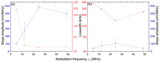
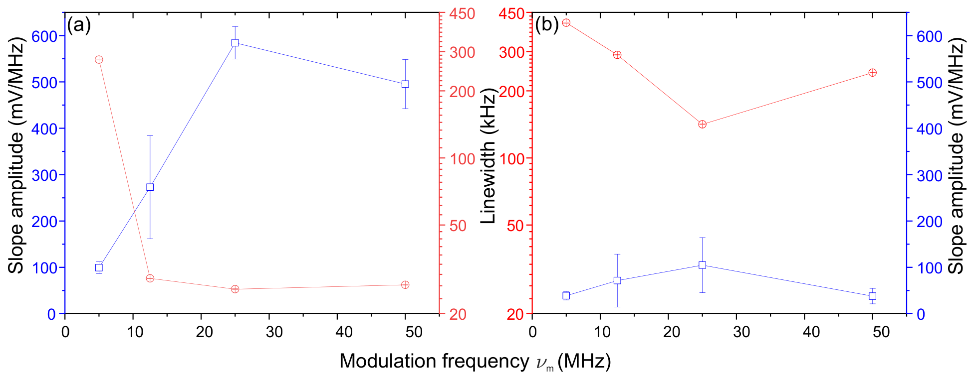
The beat note linewidths of FMS (of MTS) locking at four different modulation frequencies are plotted in Figure 6a,b. The strong correlation between linewidths and error signal slopes can be clearly seen, that is, the larger the slope, the narrower the linewidth. Eventually, the narrowest laser linewidth is $\delta {\nu }_c$ = 12.9 kHz, obtained with FMS locking of ${\nu }_m$ = 25 MHz.

Figure 6. Amplitude of error signal slope and beat note linewidth vs modulation frequency in FMS locking (a) and in MTS locking (b). The error bars of slope amplitude are the standard error of two slopes, each for one laser. The error bars of linewidth are the ones from Lorentzian fitting as stated in the caption of Figure 5.

3.3. Laser Stability

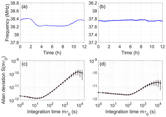
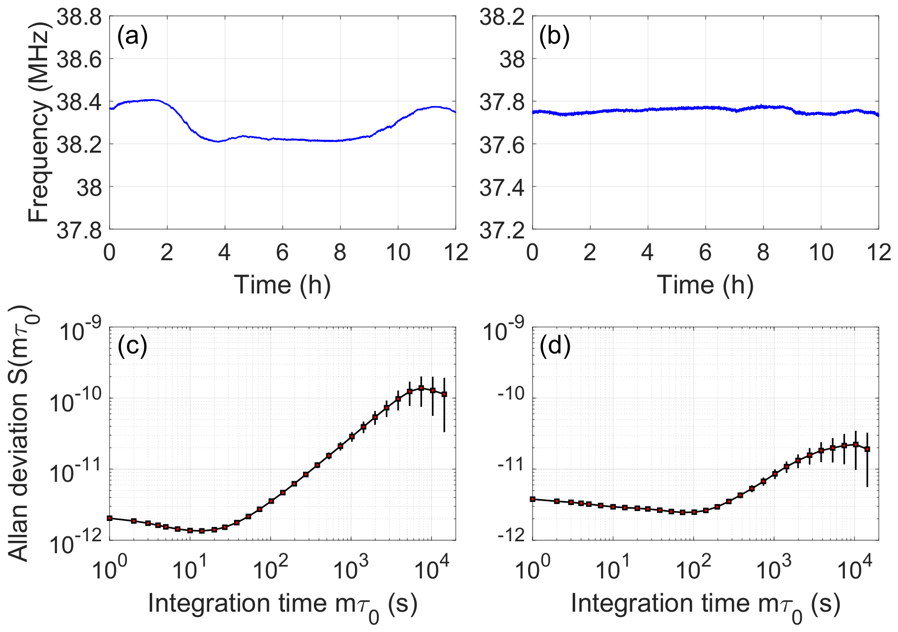
To estimate laser stability, we monitor beat notes with a frequency counter (FC), as indicated in Figure 1c and calculate the Allan deviation. Shown in Figure 7a,b are the measured beat frequencies from two FMS-locked lasers and from two MTS-locked lasers, respectively, where the frequency readings recorded by FC are binned with ${\tau }_0$ = 1 s time interval. The beat note frequency fluctuation through 12 hour duration is about 200 kHz for FMS locking and about 60 kHz for MTS locking. Laser stability can be evaluated by the fractional Allan deviation,

$$S\left(m{\tau }_0\right)={\displaystyle \frac{1}{{\nu }_c}}\sqrt{{\displaystyle \frac{1}{2(N-2m)}}\sum _{k=1}^{N-2m}{\left({\overline{y}}_{k+m}\left(m\right)-{\overline{y}}_k\left(m\right)\right)}^2},\mathrm{with}{\overline{y}}_k\left(m\right)={\displaystyle \frac{1}{m}}{\displaystyle \sum _{i=k}^{k+m-1}}{y}_i,$$

(9)

where $y_i$ is the average frequency within the ith time bin, N is the total number of time bins, and $m{\tau }_0$ is the integration time of Allan variance. Moreover, error bars are defined to be

$$SE\left(m{\tau }_0\right)={\displaystyle \frac{S\left(m{\tau }_0\right)}{\sqrt{\frac{N}{m}-1}}}.$$

(10)

Figure 7. Beat notes frequency measured by a FC for FMS locking of two lasers (a) and for MTS locking of two lasers (b). Beat note frequency stability evaluated by the fractional Allan deviation for FMS locking (c) and for MTS locking (d).

Plotted in Figure 7c,d are the fractional Allan deviations calculated from data in Figure 7a,b, respectively, with the error bars given by Equation (10). It can be clearly seen that the long-term frequency drift is considerably smaller in MTS locking than in FMS locking. This is a result of the flat baseline in the MTS error signal, as explained in Section 2.2. Although potential sources that may affect the long-term drifts of both FMS and MTS locking have not been systematically investigated, the vapor cell temperature was monitored throughout the long-term measurements and showed no significant correlation with the observed frequency drift. Eventually, the best laser stability is $S_c\left(m{\tau }_0\right)$ = 0.95$\times {10}^{-12}$ @∼10 s in FMS locking and is $S_c\left(m{\tau }_0\right)$ = 1.7$\times {10}^{-12}$ @∼100 s in MTS locking.

4. Conclusions

In this paper, we study FMS and MTS in detail, including comparing the experimental spectra to those simulated with analytical formula. Our investigation clearly demonstrates the similarity and difference in these spectroscopic techniques. Moreover, we apply both FMS and MTS for laser stabilization. With moderate efforts in optimizing parameters, we have achieved quite satisfactory locking performance: a laser linewidth of 12.9 kHz (70.8 kHz) with FMS (MTS) locking and a frequency fluctuation of 60 kHz (200 kHz) over 12 hours with MTS (FMS) locking. These results clearly show the advantages of FMS and MTS when applied for laser stabilization. Such direct comparison would be interesting to researchers, especially newcomers, working on these spectroscopic techniques and may help in making suitable choices when applying them for laser stabilization. A summary of key experimental results for MTS and FMS locking is provided in Section S5 of the Supplementary Materials. The comparison in this work currently only is for locking the Rb-87 D2 line. The generalization to other transitions and atomic species should be verified in future studies. Moreover, adding active control of the cell temperature may further improve the locking performance.

References

- Ludlow, A.D.; Boyd, M.M.; Ye, J.; Peik, E.; Schmidt, P.O. Optical atomic clocks. Rev. Mod. Phys. 2015, 87, 637–701. [Google Scholar] [CrossRef] [Scilit]
- Degen, C.L.; Reinhard, F.; Cappellaro, P. Quantum sensing. Rev. Mod. Phys. 2017, 89, 035002. [Google Scholar] [CrossRef] [Scilit]
- Brown, J.M.; Walker, T.G. Perspective: Practical atom-based quantum sensors. Phys. Rev. A 2025, 112, 040102. [Google Scholar] [CrossRef] [Scilit]
- Steane, A. Quantum computing. Rep. Prog. Phys. 1998, 61, 117. [Google Scholar] [CrossRef] [Scilit]
- Nielsen, M.A.; Chuang, I.L. Quantum Computation and Quantum Information; Cambridge University Press: Cambridge, UK, 2000. [Google Scholar]
- Mäusezahl, M.; Munkes, F.; Löw, R. Tutorial on laser locking techniques and the manufacturing of vapor cells for spectroscopy. New J. Phys. 2024, 26, 105002. [Google Scholar] [CrossRef] [Scilit]
- Hall, J.L.; Hollberg, L.; Baer, T.; Robinson, H.G. Optical heterodyne saturation spectroscopy. Appl. Phys. Lett. 1981, 39, 680–682. [Google Scholar] [CrossRef] [Scilit]
- Schenzle, A.; DeVoe, R.G.; Brewer, R.G. Phase-modulation laser spectroscopy. Phys. Rev. A 1982, 25, 2606–2621. [Google Scholar] [CrossRef] [Scilit]
- Bjorklund, G.C.; Levenson, M.D.; Lenth, W.; Ortiz, C. Frequency modulation (FM) spectroscopy. Appl. Phys. B 1983, 32, 145–152. [Google Scholar] [CrossRef] [Scilit]
- Shirley, J.H. Modulation transfer processes in optical heterodyne saturation spectroscopy. Opt. Lett. 1982, 7, 537–539. [Google Scholar] [CrossRef] [Scilit] [PubMed]
- McCarron, D.J.; King, S.A.; Cornish, S.L. Modulation transfer spectroscopy in atomic rubidium. Meas. Sci. Technol. 2008, 19, 105601. [Google Scholar] [CrossRef] [Scilit]
- Drever, R.W.P.; Hall, J.L.; Kowalski, F.V.; Hough, J.; Ford, G.M.; Munley, A.J.; Ward, H. Laser Phase and Frequency Stabilization Using an Optical Resonator. Appl. Phys. B 1983, 31, 97. [Google Scholar] [CrossRef] [Scilit]
- Bjorklund, G.C. Frequency-modulation spectroscopy: A new method for measuring weak absorptions and dispersions. Opt. Lett. 1980, 5, 15–17. [Google Scholar] [CrossRef] [Scilit] [PubMed]
- Schünemann, U.; Engler, H.; Grimm, R.; Weidemüller, M.; Zielonkowski, M. Simple scheme for tunable frequency offset locking of two lasers. Rev. Sci. Instrum. 1999, 70, 242–243. [Google Scholar] [CrossRef] [Scilit]
- Harris, S.E.; Oshman, M.K.; McMurtry, B.J.; Ammann, E.O. Proposed Frequency Stabilization of the FM Laser. Appl. Phys. Lett. 1965, 7, 185–187. [Google Scholar] [CrossRef] [Scilit]
- Eickhoff, M.; Hall, J.L. Optical frequency standard at 532 nm. IEEE Trans. Instrum. Meas. 1995, 44, 155–158. [Google Scholar] [CrossRef]
- Raj, R.K.; Bloch, D.; Snyder, J.J.; Camy, G.; Ducloy, M. High-Frequency Optically Heterodyned Saturation Spectroscopy Via Resonant Degenerate Four-Wave Mixing. Phys. Rev. Lett. 1980, 44, 1251–1254. [Google Scholar] [CrossRef] [Scilit]
- Bloch, D.; Raj, R.K.; Peng, K.S.; Ducloy, M. Dispersive Character and Directional Anisotropy of Saturated Susceptibilities in Resonant Backward Four-Wave Mixing. Phys. Rev. Lett. 1982, 49, 719–722. [Google Scholar] [CrossRef] [Scilit]
- Ducloy, M.; Bloch, D. Theory of degenerate four-wave mixing in resonant Doppler-broadened systems - I. Angular dependence of intensity and lineshape of phase-conjugate emission. J. Phys. 1981, 42, 711. [Google Scholar] [CrossRef] [Scilit]
- Ducloy, M. Doppler-free two-photon heterodyne spectroscopy by single-beam frequency modulation. Opt. Lett. 1982, 7, 432–433. [Google Scholar] [CrossRef] [Scilit] [PubMed]
- Lim, M.J.; McPoyle, S.; Cervantes, M. Modulation Transfer Spectroscopy of a four-level ladder system in atomic rubidium. Opt. Commun. 2022, 522, 128651. [Google Scholar] [CrossRef] [Scilit]
- Noh, H.R.; Park, S.E.; Li, L.Z.; Park, J.D.; Cho, C.H. Modulation transfer spectroscopy for 87Rb atoms: Theory and experiment. Opt. Express 2011, 19, 23444–23452. [Google Scholar] [CrossRef] [Scilit] [PubMed]
- Sun, D.L.; Zhou, C.; Zhou, L.; Wang, J.; Zhan, M.S. Modulation transfer spectroscopy in a lithium atomic vapor cell. Opt. Express 2016, 24, 10649–10662. [Google Scholar] [CrossRef] [Scilit] [PubMed]
- Wu, B.; Zhou, Y.; Weng, K.X.; Zhu, D.; Fu, Z.J.; Cheng, B.; Wang, X.L.; Lin, Q. Modulation transfer spectroscopy for D1 transition line of rubidium. J. Opt. Soc. Am. B 2018, 35, 2705–2710. [Google Scholar] [CrossRef] [Scilit]
- Lee, S.; Moon, G.; Park, S.E.; Hong, H.G.; Lee, J.H.; Seo, S.; Kwon, T.Y.; Lee, S.B. Laser frequency stabilization in the 10−14 range via optimized modulation transfer spectroscopy on the 87Rb D2 line. Opt. Lett. 2023, 48, 1020–1023. [Google Scholar] [CrossRef] [Scilit] [PubMed]
- Cheng, B.; Wang, Z.Y.; Wu, B.; Xu, A.P.; Wang, Q.Y.; Xu, Y.F.; Lin, Q. Laser frequency stabilization and shifting by using modulation transfer spectroscopy. Chin. Phys. B 2014, 23, 104222. [Google Scholar] [CrossRef] [Scilit]
- Wu, Y.Y.; Qin, F.J.; Ding, Z.C.; Xu, R.; Li, D.Y. Research on the Frequency Stabilization System of an External Cavity Diode Laser Based on Rubidium Atomic Modulation Transfer Spectroscopy Technology. Photonics 2024, 11, 298. [Google Scholar] [CrossRef] [Scilit]
- Zi, F.; Wu, X.J.; Zhong, W.C.; Parker, R.H.; Yu, C.H.; Budker, S.; Lu, X.; Müller, H. Laser frequency stabilization by combining modulation transfer and frequency modulation spectroscopy. Appl. Opt. 2017, 56, 2649–2652. [Google Scholar] [CrossRef] [Scilit] [PubMed]
Disclaimer/Publisher’s Note: The statements, opinions and data contained in all publications are solely those of the individual author(s) and contributor(s) and not of MDPI and/or the editor(s). MDPI and/or the editor(s) disclaim responsibility for any injury to people or property resulting from any ideas, methods, instructions or products referred to in the content. |
© 2026 by the authors. Licensee MDPI, Basel, Switzerland. This article is an open access article distributed under the terms and conditions of the Creative Commons Attribution (CC BY) license.