


Abstract
Dark-field wafer inspection systems are central to early defect detection, but the standard time (ST) of the inspection step limits throughput. We present a quantitative optimization framework that removes most of the dominant intra-tool component of ST, optical beam alignment, without equipment investment. Unlike periodic alignment and conventional fault detection and classification (FDC) monitoring, it derives the action limit of each monitored equipment parameter from a physically established beam-position tolerance at the wafer plane and applies those limits, cycle by cycle, to decide whether alignment is executed. Throughput log analysis attributed 4.0 of the 5.5 percentage-point performance loss, or 72.7%, to beam alignment. A geometric relation, calibrated empirically at two incidence angles, showed that the beam displacement from stage height deviation scales with the cotangent of the incidence angle, making shallow-incidence recipes the worst case. Over 28 days, the measured beam shift stayed within ±0.1 μm against a ±0.2 μm tolerance. Because alignment only re-centres the beam and sets no detection parameter, it can be skipped while the beam stays inside that tolerance; repeated low-angle inspections and a 300-lot production trend showed no degradation in sensitivity, matching rate, or false detection rate within the resolution of the evaluation. For the 20° standard recipe family, suppressing 80% of alignment executions on production tools lowered the median processing time from 4.16 min to 4.02 min, a 3.5% throughput gain; the interquartile range did not narrow, so the demonstrated benefit is the removal of a mean processing overhead, not a reduction in dispersion. The method applies to oblique-incidence dark-field platforms whose alignment routine only re-centres the beam; its coefficients, tolerance, and thresholds are platform-specific and must be re-measured before transfer.
1. Introduction
As semiconductor manufacturing continues to advance toward sub-10 nm technology nodes, the demand for highly sensitive and reliable inspection systems has increased sharply [1]. In particular, dark-field wafer inspection systems play a critical role in detecting micro-defects such as particles, pattern collapse, and bridging during intermediate process steps [2]. These inspection systems are deployed at key control points, including after-develop inspection (ADI), after-etch inspection (AEI), and post-chemical-mechanical-planarization inspection, where their outputs directly determine lot disposition decisions such as hold, rework, or release. Consequently, the performance and stability of inspection tools are directly linked to yield, process control, and overall manufacturing productivity. The optical principles that govern the illumination and collection paths of such systems are treated comprehensively in the standard references [3,4].
However, as process complexity increases, maintaining consistent inspection performance across tools has become increasingly challenging. One of the most critical limitations is the excess of the realized standard time (ST) over its assigned value, since ST governs inspection throughput and equipment utilization. Queueing-theoretic treatments of manufacturing systems show that the mean waiting time at a workstation depends on both the mean process time and its coefficient of variation, so that the mean and the dispersion of ST each determine effective capacity at high utilization [5,6,7], and both have been targets of fab-level release and scheduling control [8,9]. In high-volume manufacturing environments, even a small excess time per wafer therefore accumulates into measurable capacity loss [10,11]. In practice, average processing time (APT) is frequently observed to exceed the assigned standard, and to vary, not only across nominally identical tools but also within the same tool over time. The present work addresses the mean component of this excess, that is, the recurring overhead that a fixed procedural step adds to every inspection cycle; the dispersion component is characterized but not reduced, and is identified as follow-up work.
Among the various components of the inspection sequence, optical beam alignment is a fundamental operation required to maintain the accuracy of the optical system. Conventional inspection strategies assume that beam alignment must be executed prior to inspection to ensure consistent detection sensitivity; on the platform evaluated in this study, it is triggered whenever the inspection recipe changes and, otherwise, on a fixed period of approximately one hour. As a result, beam alignment is repeatedly performed regardless of actual system stability, introducing additional overhead into the inspection process. Despite its widespread use, the necessity of performing beam alignment under all conditions has not been rigorously evaluated from a quantitative or system-level perspective.
Our previous study on the same class of dark-field platform addressed the opposite end of the performance trade-off, optimizing illumination polarization, wavelength, and incidence angle to lower the detection limit for 30 nm particles [12]. The present work is independent in execution and scope: it targets throughput rather than sensitivity, uses production throughput logs and equipment monitoring data rather than electromagnetic simulation, and reports results obtained on a different set of production tools. No text or datasets from [12] are reproduced in this manuscript, and neither the constants nor the conclusions of the two studies are interchangeable: the earlier work characterized detection sensitivity, whereas the present work characterizes throughput on a different set of production tools.
The technical contributions of this work are threefold. First, it decomposes the measured ST loss of a production dark-field inspection fleet into its constituent operations and quantifies the share attributable to beam alignment. Second, it establishes a geometric tolerance criterion linking stage height deviation, incidence angle, and beam displacement at the wafer plane, and calibrates that criterion against tool measurements [13]. Third, it demonstrates a conditional-execution scheme, built on fault detection and classification (FDC) infrastructure, on production tools and reports the resulting change in the APT distribution together with the detection-performance evidence that supports it.
The distinction from existing practice should be stated explicitly. Periodic or recipe-triggered alignment, the current industrial norm, is a time-based rule: it executes on a schedule regardless of whether the beam has moved, so it simultaneously wastes executions while the optics are stable and leaves a genuine excursion uncorrected until the next scheduled run. Standard FDC monitoring, in turn, is a surveillance function: it compares equipment parameters against control limits and raises alarms or interlocks for maintenance, but it neither relates those parameters to the optical quantity that governs detection nor modifies the inspection sequence itself. The framework proposed here differs from both in three respects. First, it identifies its target quantitatively, by decomposing the measured ST loss and showing that a single intra-tool operation accounts for 72.7% of it. Second, it replaces the time-based rule with a physical one: the action threshold of each monitored parameter is derived, through the calibrated geometric relation of Equation (1) and the measured thermal and pressure couplings, from the beam displacement that the parameter produces at the wafer plane, so that the execution decision is taken against a beam-position tolerance that was itself established by direct detection testing. Third, it uses the FDC infrastructure as a control input rather than as an alarm channel—the decision is taken before every inspection cycle and acts on the sequence directly—so that the number of executions falls while the worst-case interval between a disturbance and its correction becomes shorter, not longer (Section 4.2). To the best of the authors’ knowledge, a conditional-execution scheme for an optical calibration step that is derived from production throughput data, tied to a physical beam-position tolerance, and validated on production tools has not previously been reported for dark-field inspection systems. The claim of generality is a claim about this structure and about the physical conditions that make it valid—a calibration step that is positional rather than parametric, a monitored quantity that can be mapped onto it, and monitoring fast enough to decide on it—rather than an empirical claim about other tool types; Section 4.3 states those conditions, the measurements required for a transfer, and the cases in which the method should not be transferred at all.
Collectively, these contributions provide a comprehensive framework that integrates production-data analysis, optical modeling, and condition-based equipment control into a unified throughput optimization strategy. Beyond the specific application investigated in this study, the proposed methodology also illustrates how equipment monitoring and physics-based decision-making can be combined to improve manufacturing productivity without additional hardware investment or modification of inspection recipes. Figure 1 places the inspection step within the overall process flow, which clarifies why inspection standard time translates directly into screening capacity.
Figure 1.
Position of the inspection step within the semiconductor process flow and the principal measurement categories of the metrology and inspection sector. The inspection branch (left) covers wafer-level defect detection and defect review, whereas the metrology branch (right) covers thickness, critical dimension (CD), structure, and overlay measurement.
Figure 1 distinguishes the inspection step from the adjacent metrology operations. Inspection tools generate wafer-level defect maps and feed defect review, whereas metrology tools return thickness, critical dimension, structure, and overlay values. Because inspection results are used for lot disposition rather than for parametric process control, inspection throughput directly constrains how much material can be screened, and any reduction in inspection standard time is realized immediately as additional screening capacity. Within the inspection sequence itself, beam alignment is primarily responsible for maintaining the positional accuracy of the illumination beam on the wafer surface. However, beam position can be influenced by various factors, including mechanical variations such as stage Z-height deviation, as well as environmental fluctuations such as temperature and atmospheric pressure. These factors introduce potential beam shifts, which may affect defect detection sensitivity if not properly controlled.
In this study, we challenge the conventional assumption that beam alignment must always be executed and propose a quantitative optimization framework that enables selective skipping of beam alignment operations under controlled conditions. Through production throughput log analysis, beam alignment was identified as the dominant contributor to inspection performance loss, accounting for 72.7% of the measured loss, motivating a detailed investigation into its necessity and impact on inspection performance. A physics-based analysis was conducted to evaluate beam position shifts induced by mechanical and environmental variations. The analysis shows that, within a defined tolerance range of ±0.2 μm at the wafer plane, beam alignment can be omitted without an observable change in detection performance. Based on this finding, a monitoring-based control framework is proposed, in which critical parameters such as stage position, temperature, and pressure are continuously tracked to determine whether beam alignment is required. The proposed approach integrates data-driven monitoring with a real-time decision logic that selectively skips alignment operations while holding the beam inside its validated positional envelope. Experimental validation was performed on production inspection tools in a high-volume semiconductor manufacturing environment. The results demonstrate that the proposed method suppresses about 80% of the beam-alignment executions and, with them, most of the beam-alignment component of ST, and improves throughput for the 20° standard recipe family without an observable change in defect detection performance; the benefit is a reduction of the mean processing overhead, not of its dispersion. By shifting from a conservative, always-execute strategy to a condition-based control paradigm, the proposed framework provides a practical and scalable direction for data-driven optimization of inspection equipment in advanced semiconductor manufacturing environments.
2. Beam Alignment Variability Analysis and Conditional Execution Strategy
2.1. Standard Time (ST) Loss Decomposition and APT Distribution Analysis
In high-volume semiconductor manufacturing, inspection throughput is a critical factor that directly impacts equipment productivity and overall fab efficiency. Standard time (ST), defined as the total time required to complete a single inspection sequence, serves as a key performance metric for evaluating tool efficiency. In practice, ST is composed of multiple sequential operations, including wafer loading, stage movement, optical setup, beam alignment, and defect scanning. Tool efficiency is expressed here as performance availability, defined as the ratio of the standard ST assigned to the step to the median processing time actually realized, a performance term of the same kind as those used in overall equipment effectiveness [14,15]; the median is used as the central statistic because it is insensitive to the residual outliers that survive the trim described below. For the step examined here, the assigned standard ST was 3.83 min; throughout the paper, quoted times are rounded to 0.01 min and quoted percentages to 0.1 point, while all ratios are computed from the unrounded values.
Because the standard-time assignment rule derives the standard value from the faster part of the observed APT population after ±2σ outlier removal, performance availability is structurally capped at 97.5% under the distribution shape observed on this fleet; the residual 2.5% is a property of the assignment rule as applied, not of the equipment. The standard value is frozen at recipe qualification and was not re-derived after the intervention, so the same cap applies to both evaluation windows compared in this study.
To quantify the excess of realized ST over the assigned standard, together with its spread, we analysed the average processing time (APT) across a fleet of 20 production dark-field inspection tools operating under identical process conditions. The dataset comprised every lot of a single standard group and process program identifier, belonging to the 20° standard recipe family (Section 3.1), processed over a 20-day window, with outliers beyond ±2σ of the mean APT removed before analysis. The resulting per-wafer APT population is summarized as an interquartile interval in Figure 2; the full frequency distribution was not retained. Tools were deployed at in-line inspection checkpoints such as ADI, AEI, and post-chemical-mechanical-planarization inspection. Despite nominally identical configurations, a spread of 0.30 min between the first and third quartiles of the per-wafer APT population was observed. This pooled spread combines within-tool and between-tool components, which the present dataset does not separate; a variance decomposition is identified as future work in Section 4.4. The APT population thus sat well above the assigned standard and showed a substantial spread, and because inspection steps are executed repeatedly for every lot, wafers processed in the slow tail of this spread accumulate a disproportionate share of the throughput loss. The scattering measurement that the inspection step performs, and the spatial filtering it relies on, are described in [16,17]. Figure 2 summarizes the baseline APT statistics and the loss decomposition derived from them.
Figure 2.
Standard-time performance of the dark-field inspection fleet before optimization. (a) Interquartile interval of the per-wafer APT population, pooled over the 20 tools of the fleet and over every lot of the selected standard group and process program in the 20-day window, (Q1 = 4.02 min, median 4.16 min, Q3 = 4.32 min) against the assigned standard ST of 3.83 min; the shaded region is the 0.33 min gap between the two, corresponding to a performance availability of 92.0%. Whiskers are omitted because the full range of the population was not retained. (b) Pareto decomposition of the 5.5 percentage-point performance loss into its constituent operations. Bars give the contribution of each operation class in percentage points (orange, intra-tool; blue, tool-to-tool), and the line, read on the right-hand axis, gives the cumulative share of the 5.5-point total. Beam alignment is the only intra-tool term and accounts for 4.0 points, or 72.7% of the total; the three tool-to-tool terms—alignment search failure, autofocus, and loading position—contribute 0.75, 0.50, and 0.25 points, respectively.
Two properties of this dataset should be defined precisely, because they determine how the summary statistics may be read. First, the fleet is homogeneous: the 20 tools are units of the same dark-field platform and model configuration supplied by one vendor, with the same illumination and collection hardware, the same recipe set, and the same maintenance specification, and they differ only in installation date, maintenance history, and the accumulated wear that preventive maintenance is intended to bound. The results reported here therefore characterize one tool type, and unit-to-unit variability enters only through those secondary differences. Second, the word average in average processing time refers to two nested operations, and the population summarized in Figure 2a pools both. The tool reports, for each lot, the processing time per wafer averaged over the wafers of that lot; the population is then formed from these per-lot values over every lot of the selected standard group and process program processed in the window by any of the n = 20 tools. Averaging is thus performed over wafers within a lot and pooled over lots and over tools, and the quoted quartiles are order statistics of that pooled population rather than of a per-tool mean. The number of independent equipment units is 20, which is the relevant count whenever the between-tool component is at issue. Because the per-record data were not retained (Appendix A), no confidence interval is attached to the quartiles, and the differences reported in Section 3.3 are stated as observed shifts of the pooled distribution rather than as tested effects.
The 20-day length of the window was set by the reporting and maintenance cadence of the line rather than by a statistical stopping rule, and this should be stated plainly. Twenty production days is the standard reporting period of the fab; it spans a complete rotation of the product mix within the selected standard group; and it exceeds the preventive-maintenance interval of the platform, so that every tool contributes lots from both freshly maintained and end-of-interval states. Since the baseline alignment period is approximately one hour, the window is more than two orders of magnitude longer than the interval between alignment events, and each tool contributes several hundred of them. The same length, the same product restriction, and the same ±2σ trim were applied to the post-deployment window of Section 3.3, so that any residual dependence on window length acts in the same direction on both populations and largely cancels in the comparison. What this design does not provide is a sensitivity analysis over alternative window lengths: the archived logs retain the per-window summaries rather than the per-record data, so the quartiles cannot be recomputed for sub-windows or for shifted windows, and the insensitivity of the reported statistics to the choice of window is therefore argued from the matched design rather than demonstrated. A rolling-window analysis on prospectively retained records is identified as future work in Section 4.4.
Figure 2a summarizes the per-wafer APT population before optimization through its quartiles. The measured APT population had a median of 4.16 min with a first quartile of 4.02 min and a third quartile of 4.32 min. Over the same window, the measured performance availability of the fleet was 92.0% against the structural ceiling of 97.5%, leaving a performance loss of 5.5 percentage points. The 0.30 min interquartile spread indicates, in addition, that inspection performance was not uniformly maintained across the fleet, which complicates production scheduling and capacity utilization; this spread is characterized here but, as shown in Section 3.3, it is not the quantity that the proposed framework reduces.
Figure 2b resolves the 5.5-point loss into its constituent operations. The chart is a Pareto decomposition: each bar is the contribution of one operation class to the performance loss, in percentage points; the bar colour distinguishes the intra-tool term from the tool-to-tool terms; and the line, read on the right-hand axis, gives the cumulative share of the 5.5-point total (72.7%, 86.4%, 95.5%, and 100%). The contributions were obtained as follows. Each operation class was identified from the step-level timestamps in the equipment throughput logs of the 20-tool fleet over the 20-day baseline window; its accumulated time was summed over all lots in the window, and the sum was expressed as a fraction of the available operating time. Because performance availability is itself a ratio of times, this fraction is directly the number of percentage points by which the operation lowers availability. The four classes together account for the full 5.5-point gap between the 97.5% ceiling and the measured 92.0%, so the decomposition is exhaustive at the resolution of the logged step boundaries. It is a decomposition of the mean loss; no variance decomposition was performed.
The decomposition attributed 0.75 percentage points to alignment search failures, 0.50 points to autofocus, 0.25 points to loading-position error, and 4.0 points to beam alignment. The first three are tool-to-tool terms: they arise from the mechanical or optical state of an individual tool, differ from tool to tool, and are already bounded by preventive maintenance, so they cannot be reduced further by a procedural change. Beam alignment is different in kind. It is an intra-tool term, recurring within every tool regardless of its maintenance state, because it is triggered by the recipe change and by the fixed timer described in Section 1 rather than by any drift of the tool; it accounted for 4.0/5.5 = 72.7% of the total loss [18]. This distinction is what makes the decomposition actionable: the largest term is also the only one that a change of procedure, as opposed to hardware maintenance, can remove.
The current practice of executing beam alignment on every recipe change and on a fixed period introduces redundant operations whenever the optical system is in fact stable. This conservative approach, while ensuring alignment accuracy, adds a recurring overhead to the mean inspection time; whether it also contributes to the dispersion of APT was not measured in this dataset and is not claimed here. Beam alignment therefore represents the single largest opportunity for reducing the mean ST loss. Based on these observations, it becomes evident that reducing or selectively eliminating unnecessary beam alignment operations can improve inspection efficiency. However, such an approach requires a rigorous understanding of the underlying optical mechanisms and the conditions under which alignment can be safely skipped without compromising detection performance. This motivates a detailed analysis of the beam alignment process and its sensitivity to mechanical and environmental variations, which is presented in the following section [19,20].
2.2. Optical Beam Alignment Mechanism and Sensitivity Factors
Optical beam alignment in dark-field wafer inspection systems is a critical process that ensures the accurate positioning of the illumination beam on the wafer surface. Proper alignment is required to maintain consistent scattering signal intensity from defects, which directly influences detection sensitivity and inspection reliability; the scattering of light by particles and defects on a wafer surface, and its dependence on the illumination geometry, is treated in [21,22,23]. The alignment process compensates for positional deviations in the optical path, which may arise from mechanical tolerances and environmental fluctuations during system operation. In a typical dark-field inspection system, the illumination beam is projected onto the wafer at a specific incident angle, and scattered light from defects is collected by the detection optics and integrated on a time-delay-integration (TDI) sensor [24,25]. On the evaluated platform, alignment is executed by translating a motorized angle mirror along the axis transverse to the beam until the scattered-light profile is re-centred on the sensor, using a ceramic reference block mounted on the stage chuck. The accuracy of this process depends on the precise positioning of the beam relative to the wafer surface. Any deviation in beam position, commonly referred to as beam shift, can lead to variations in the scattering signal and potentially degrade defect detection performance [26]. The coupling is radiometric rather than parametric: the TDI sensor integrates scattered light from a fixed projected area on the wafer, so a lateral displacement of the illumination profile changes the local irradiance delivered to that area and hence the scattered power collected from a defect within it, while leaving every detection setting of the recipe untouched. Figure 3 shows the corresponding optical arrangement and the two error paths it must control.
Figure 3.
Optical mechanism of beam alignment in a dark-field inspection system. The illumination beam is folded by a steerable angle mirror onto the wafer surface, and the scattered light is imaged onto a time-delay-integration (TDI) sensor. Two error paths are indicated: ① a focus position shift arising from stage Z-height deviation, and ② a beam position shift at the wafer plane, which the angle mirror compensates for through the lateral shift action shown.
Figure 3 illustrates the optical architecture of the inspection system and the factors that induce beam position shift within it. The illumination beam is folded by a mirror pair, passes through the beam-forming lens, and is directed onto the wafer at the recipe-defined incidence angle; scattered light is collected by the objective group and integrated on the TDI sensor, whose projected area on the wafer defines the effective inspection swath. As shown in the figure, beam shift can be caused by multiple sources, including mechanical variations such as stage Z-height displacement, as well as environmental factors such as temperature changes and atmospheric pressure fluctuations. These variations affect the optical path length and alignment geometry, resulting in positional deviations of the illumination beam on the wafer surface, and are corrected by the lateral shift action of the angle mirror.
Among these factors, stage Z-height variation plays a particularly important role, as it directly alters the focal position and beam incidence geometry. The geometric origin of the effect is simple. For an illumination beam incident at an angle θ measured from the wafer surface, raising the wafer by ΔZ shortens the path of the beam to the surface by ΔZ/sin θ, and because the beam travels at the angle θ to the surface, the illuminated spot moves along the surface by (ΔZ/sin θ)·cos θ = ΔZ·cot θ. In pure free-space geometry, with a fixed illumination column and an exact measurement of the surface height, a stage height deviation ΔZ therefore displaces the illuminated spot laterally by
where Δx is the lateral displacement of the illumination spot at the wafer plane, and k is a dimensionless coupling coefficient, equal to unity in the free-space case just described. On a real tool, k absorbs every departure from that idealization—in particular the relation between the height signal actually monitored and the true excursion of the wafer surface, and any motion of the illumination path that is common with the stage—and it is therefore treated in this work as an empirical constant to be calibrated, not as a derived quantity. Equation (1) was calibrated against tool measurements at two operating points: a stage height deviation of ΔZ = 1.8 μm produced a lateral beam displacement of 2.5 μm at θ = 20° and 17.2 μm at θ = 3°, that is, 1.39 and 9.56 μm per micrometre of height deviation. As shown in Figure 4a, a single constant k = 0.5 reproduces both measurements to within 1.1% (predicted 1.37 and 9.54 μm/μm), and the measured ratio 2.5/17.2 = 0.145 matches the predicted cot 20°/cot 3° = 0.144 to within 1%. Two features of this calibration should be stated plainly. First, it rests on two incidence angles and a single height deviation, so it fixes k for this platform but does not test the cotangent form against other monotonic angle dependences; k = 0.5 is an empirical calibration value, not a verified physical constant. Second, the value is one half of the free-space prediction k = 1. The physical origin of this factor has not been established experimentally in the present study. The most plausible explanation, adopted here as a working hypothesis, is that the monitored height signal is the autofocus servo position rather than an independent measurement of the wafer surface: the illumination column partially follows the stage Z motion, so that the beam displacement realized at the wafer plane is roughly one half of the free-space value for the same servo-reported height change. Other contributions, such as common-mode motion of the optical mounts with the stage, cannot be excluded with two operating points. The angular scaling, which is the property used in this work, is unaffected by the value of k; the origin of the factor is listed as a limitation in Section 4.4, together with the independent surface-height measurement and incidence-angle sweep that would resolve it. Equation (1) should therefore be read as calibrated against, rather than verified by, the two available operating points. The practical consequence is that shallow-incidence recipes are the worst case by a factor of approximately seven, so the tolerance analysis must be anchored to the lowest incidence angle in the recipe set rather than to the nominal condition.
Δx = k · ΔZ · cot θ
Figure 4.
Feasibility of conditional beam alignment under controlled mechanical and environmental stability. (a) Equation (1) evaluated with the empirically calibrated coefficient k = 0.5 (two operating points; Section 2.2) against the two measured incidence angles; the predicted displacement per unit stage height deviation reproduces the measured 1.39 μm/μm at 20° and 9.56 μm/μm at 3° to within 1.1%. (b) Error budget at the 20° nominal incidence angle: the stage-height term of Equation (1) at the observed ±0.1 μm, the thermal term at the measured 0.2 μm/°C over the observed 0.5 °C, the pressure term of Equation (3) over the ±5 hPa monitoring band, their root-sum-square, and the directly measured beam shift, all against the ±0.2 μm tolerance. The directly measured value lies below the summed bound, indicating partial cancellation. (c) Observed variation of the three monitored parameters and of the beam-position criterion, shown against the respective thresholds of Table 1; a threshold crossing triggers execution of the alignment. (d) Beam position movement measured over the three-week alignment-free interval for the mid and low illumination channels, against the ±0.2 μm tolerance band.
For the same reason, the way in which Δx is obtained should be stated explicitly, since it determines what k does and does not represent. The lateral displacement is not measured at the wafer plane with an independent probe. It is obtained during the alignment routine from the position of the illumination spot on the TDI sensor, which is converted to an equivalent displacement at the wafer plane through the magnification of the collection path and the sensor pixel pitch; the routine reports the result in micrometres referred to the wafer plane, and it is this quantity that is plotted in Figure 4d, listed in Table 1, and compared with the ±0.2 μm tolerance. The sensor-to-wafer-plane conversion is a fixed property of the collection optics and is applied before Equation (1) is evaluated. Consequently, k is not the calibration factor of the TDI unit. It is the dimensionless ratio between the wafer-plane displacement obtained in this way and the free-space geometric prediction ΔZ·cot θ computed from the monitored height signal, so it quantifies the coupling between the monitored signal and the realized displacement, not the conversion between sensor counts and micrometres. The distinction matters in one direction: a systematic error in that conversion would be absorbed into k and could not be separated from a genuine optical coupling with the two operating points available. This is a further reason for treating the factor of one half as a hypothesis rather than an established mechanism, and the independent surface-height measurement proposed in Section 4.4 would also yield an uncertainty for the conversion itself.
Table 1.
Beam-position tolerance criterion, the FDC action thresholds, the variation observed during the evaluation window, and the beam displacement that the observed variation implies at the 20° nominal incidence angle (20° standard recipe family; see Section 3.1 for the scope of validity). The first row is the acceptance criterion; the remaining three rows are the signals monitored in real time. The root-sum-square of the three contributions is 0.171 μm, against a directly measured beam shift of ≤0.1 μm; the pressure entry is evaluated conservatively at the full ±5 hPa band rather than at the observed variation.
Similarly, temperature variation leads to thermal expansion of the optical mounts, displacing the optical centre by
where α is the linear thermal expansion coefficient of the mount material and L the relevant mechanical path length, while temperature and pressure fluctuations also modify the refractive index of the air along the optical path according to
ΔL = α · L · ΔT
Δ(nL) = L · (∂n/∂T · ΔT + ∂n/∂P · ΔP)
The two derivatives of Equation (3) are not fitted here. They are evaluated at the 355 nm illumination wavelength from the Ciddor equation [27] and cross-checked against the updated Edlén equation [28], which agree to better than 1% over the temperature and pressure range monitored in this work. Near 20 °C and 1013 hPa, this gives ∂n/∂P ≈ 2.7 × 10⁻⁷ hPa−1 for air in the ultraviolet and, since the refractivity of air is proportional to density at fixed composition, ∂n/∂T = −(n − 1)/T ≈ −9 × 10⁻⁷ K−1. A tool-side correlation study gave a beam displacement of 0.57 μm across a full 1000 hPa change in ambient pressure, so that the pressure term contributes less than 0.01 μm over the ±5 hPa monitoring band of Table 1, more than an order of magnitude below the alignment tolerance; the pressure term of Equation (3) is therefore not the limiting contribution. The thermal term of Equation (2) was likewise bounded experimentally, by the temperature-forcing evaluation described in Section 2.3, rather than computed from α and L, which are not independently characterized for this mount assembly. Over the monitored operating envelope, the geometric term of Equation (1) is the largest single term in the error budget. Despite these potential sources of variation, the magnitude of beam shift under normal operating conditions is therefore bounded within a limited range.
To evaluate the impact of beam shift on inspection performance quantitatively, a sensitivity analysis was conducted by examining the relationship between beam displacement and defect detection response. That analysis, described in Section 2.3 and summarized in Table 2, indicates that within a defined tolerance range, no change in the detection response is observed, suggesting that the system exhibits inherent robustness against small alignment deviations. This observation challenges the conventional assumption that beam alignment must be executed prior to every inspection cycle. If the beam position remains within an acceptable tolerance band, repeated alignment operations may not be necessary to maintain detection performance. Instead, alignment can be conditionally executed only when system variations exceed predefined thresholds. Therefore, the key question is not whether beam alignment is required, but under what conditions it can be safely skipped. To answer this, it is essential to define the allowable tolerance range for beam position and to evaluate the stability of the system under realistic operating conditions. This leads to the feasibility analysis of conditional beam alignment, which is discussed in the following section [29,30].
Table 2.
Summary of the detection-performance checks that support the ±0.2 μm beam-position tolerance and the conditional-execution scheme. Outcomes are reported at the level retained in the archived dataset; individual per-repeat metric values and the numerical response at each offset step were not retained (see text).
2.3. Feasibility of Conditional Beam Alignment Under Controlled Conditions
Based on the analysis of beam alignment mechanisms and the sensitivity of defect detection to beam position variations, we investigate the feasibility of selectively skipping beam alignment operations under controlled conditions. While conventional inspection procedures mandate alignment prior to each inspection cycle to ensure consistent performance, the results of the previous section indicate that the inspection system tolerates small beam position deviations. To evaluate this feasibility quantitatively, we define a tolerance band for allowable beam shift within which no change in the defect detection response is observed [31].
The ±0.2 μm tolerance used in this study should be interpreted as an equipment-specific empirical acceptance band rather than as a universal optical limit. It was established by deliberately applying incremental offsets to the angle mirror and monitoring, at each offset, the scattered-light profile on the TDI sensor and the inspection response of the recipe. The acceptance boundary was defined as the largest beam-position deviation for which the scattered-light profile remained within the equipment control limits and no change was observed in the evaluated detection metrics; the procedure and its outcome are summarized in Table 2 (Section 3.4), and the resulting tolerance region is shown together with the sensitivity of the beam displacement to each monitored parameter in Figure 5 (Section 3.1). Beam shifts of up to ±0.2 μm at the wafer plane were not associated with an observable change in the evaluated detection metrics, whereas excursions beyond that band moved the scattered-light profile outside its control limits, so the boundary is located by measurements on both sides of its edge rather than by extrapolation. Because the tolerance depends on the optical magnification, illumination footprint, sensor projection, and recipe geometry of the evaluated platform, it should be re-established before application to another tool family or incidence-angle configuration.
Figure 5.
Sensitivity of the beam displacement at the wafer plane to each monitored parameter, with the ±0.2 μm tolerance region shaded and the FDC action thresholds of Table 1 marked. (a) Geometric term of Equation (1) evaluated with k = 0.5, for the nominal 20° recipe family and for the 3° low-angle recipe; the tolerance is reached at ΔZ = 0.144 μm at 20° and at 0.021 μm at 3°. (b) Environmental terms of Equations (2) and (3): chamber temperature at 0.2 μm/°C (lower axis) and ambient pressure at 0.57 μm per 1000 hPa (upper axis). (c) Combined error budget at the action thresholds and over the observed operating envelope, showing the individual contributions, their root-sum-square, and the displacement measured directly on the sensor. Markers denote the variation observed during the evaluation.
The environmental threshold of Table 1 was established by the same forcing method: the internal air-handling fan speed was varied to drive the chamber temperature away from its setpoint, and the beam position was re-measured at each level, which located the onset of scattered-profile drift at approximately ±1 °C. Two independent forcing paths thus place the edge consistently: the direct mirror-offset test locates it at ±0.2 μm of beam displacement at the wafer plane, and the temperature-forcing evaluation places the onset of scattered-profile drift at approximately ±1 °C, which at the measured coupling of 0.2 μm/°C corresponds to the same ±0.2 μm displacement. During the 28-day production evaluation, moreover, the beam shift measured directly on the sensor remained at or below ±0.1 μm, so normal operation engages at most one half of the acceptance band.
It is worth stating the logic of the safety argument explicitly at this point, because it is positional rather than statistical. Beam alignment sets no detection parameter: it only returns the illumination beam to its reference position on the sensor. Detection sensitivity is a function of where the beam is, not of whether the alignment routine was executed. Omitting the alignment step is therefore not expected to alter the detection outcome, provided that the beam position and the relevant optical conditions remain within the validated operating envelope, and executing it when the beam is already centred returns the same position and changes nothing except the elapsed time. The evidence that matters is therefore the beam-position evidence, and the detection comparisons reported in Section 3.4 are confirmatory.
Figure 4 illustrates the feasibility of conditional beam alignment under controlled mechanical and environmental stability conditions. When the key system parameters remain within predefined bounds, beam displacement remains within the acceptable tolerance range, and beam alignment can be omitted without an observable change in inspection performance. As illustrated in Figure 4, the observed variations of the monitored parameters remain below their respective action thresholds, providing operational margin for conditional beam alignment. The combined error budget, including stage height deviation, chamber temperature variation, and ambient pressure fluctuation, remains within the predefined beam-position tolerance under normal production conditions. Consequently, the optical system maintained a stable illumination geometry throughout the evaluation period, indicating that routine beam alignment provides no additional benefit while the monitored parameters remain within their allowable ranges.
To validate this approach, a long-term stability analysis was conducted under typical production conditions. Key parameters influencing beam alignment, including stage Z-height variation, temperature drift, and pressure fluctuation, were continuously monitored on four tools over a 28-day period. The observed variations remained within the defined tolerance limits throughout: stage Z-height stayed within ±0.1 μm and chamber temperature varied by less than 0.5 °C. Ambient pressure is evaluated as the change within a single inspection cycle rather than as an absolute level, since the barometric level itself moves by tens of hectopascals over a month; on that basis, the per-cycle excursion stayed below 1 hPa. By Equation (1), a stage height deviation of ±0.1 μm corresponds to a beam displacement of 0.14 μm at the 20° nominal incidence angle, approximately 70% of the ±0.2 μm tolerance band, and the beam shift measured directly on the sensor likewise stayed within ±0.1 μm. An independent check was performed over a three-week interval for both of the platform’s illumination channels, the mid-angle and the low-angle path: the beam position recorded at the start of the interval was compared with that recorded at the end without any intervening realignment, and the movement was zero for the mid channel and 0.010–0.015 μm for the low channel, at most 8% of the tolerance band (Figure 4d).
The impact of alignment skipping on defect detection performance was evaluated separately, using the 3° extreme low-angle recipe identified by Equation (1) as the worst case, with three repeated inspections per condition; the 3° recipe was chosen for this check precisely because the geometric margin of Table 1 does not extend to it (Section 3.1), so that a null result there is the most demanding one available. Across the three repeated inspections performed for each condition, detection sensitivity, matching rate, and false detection rate showed no degradation beyond the repeat-to-repeat range of the measurement when beam alignment was omitted. In addition, the 300-lot production trend collected over the two months following deployment showed no systematic shift in defect-capture behaviour. The scope and outcome of these checks are tabulated in Section 3.4 (Table 2). These results provide confirmatory operational evidence within the evaluated sample, but they should not be interpreted as a formal statistical demonstration of equivalence.
These observations indicate that the alignment process, while essential under unstable conditions, is not always required during steady-state operation. They support a conditional alignment strategy, in which beam alignment is executed only when system conditions exceed predefined thresholds. By eliminating unnecessary alignment operations, this approach directly reduces the mean inspection time and contributes to improved throughput, while the monitoring of the stability parameters keeps the beam inside its validated positional envelope. The feasibility of conditional beam alignment is therefore supported both by the optical sensitivity analysis and by the production data [32], and it establishes the foundation for the monitoring-based control framework presented in the following section [33,34].
3. Experimental Configuration and Results Analysis
3.1. Tools, Dataset, and Evaluation Protocol
All measurements were performed on production dark-field wafer inspection tools of a single platform family operating in a high-volume memory fabrication line. The illumination source is a 355 nm ultraviolet solid-state laser; the beam is attenuated, expanded, and folded onto the wafer by a motorized angle mirror, and the scattered light is collected onto a TDI sensor. Two illumination geometries were evaluated, with distinct roles. The standard recipe family at an incidence angle of 20° measured from the wafer surface is the family on which the conditional-execution scheme was deployed and on which the throughput evaluation was performed. An extreme low-angle recipe at 3°, which Equation (1) identifies as the worst case for height-induced beam displacement, was used only for the detection-robustness check described in Section 3.4; it was not operated under conditional execution in production.
Three datasets were used. First, throughput logs from the same fleet of 20 tools (the homogeneous fleet of identical units described in Section 2.1) were used for the ST decomposition and the APT summaries: a 20-day baseline window, restricted to a single standard group and process program identifier of the 20° standard recipe family, provides the pre-optimization population of Figure 2. Second, a feasibility set acquired on 4 tools monitored continuously for 28 days was used for the long-term stability evaluation of Figure 4; that length was chosen so that the monitoring interval would exceed the baseline alignment period of approximately one hour by more than two orders of magnitude and would contain at least one preventive-maintenance event on every monitored tool, and it embeds the three-week alignment-free interval reported in Section 2.3. The criteria used to select the 20-day throughput windows, and the limits of what a non-concurrent matched design can establish, are set out in Section 2.1. Third, real-time FDC traces from the monitored fleet were used for the monitoring evaluation of Figure 6. A second 20-day window collected after deployment under the same product restriction provides the post-deployment population of Figure 7, so the two throughput windows are matched on product content but are not concurrent. Detection performance was confirmed separately on the 3° recipe with three repeated inspections per condition, and by a mass-production trend covering 300 lots over two months (Section 3.4, Table 2). Certain production-related numerical values have been normalized for confidentiality purposes.
Figure 6.
FDC-based real-time monitoring used for the beam alignment decision, shown across the monitored production fleet; tool identifiers and internal parameter names have been removed from the plots. (a) Chamber temperature over a 22 h window; each trace is one monitored temperature signal, and although the fleet spans 22.7–24.1 °C, the within-tool variation is far below the action threshold, which is applied to the deviation of each tool from its own baseline rather than to an absolute level. (b) Stage Z-height reported by the autofocus system in the tool’s native encoder units over a 2.5-day window; each trace is one tool, and no drift is resolvable at the plotted scale. The encoder-to-micrometre conversion is tool-specific and is not disclosed here; the quantitative check against the ±0.14 μm threshold is made on the converted signal inside the FDC system.
Figure 7.
Effect of the proposed conditional alignment framework. (a) Interquartile interval of the per-wafer APT population for the baseline and the proposed state; every quartile moves to a shorter time, with the median falling by 0.14 min and Q1 and Q3 by 0.17 and 0.14 min; the interquartile range does not narrow (0.30 min before, 0.33 min after), so the distribution is shifted, not compressed. (b) Recovery of the beam-alignment loss term: suppressing 80% of the alignment executions raises performance availability from 92.0% to 95.2% against the 97.5% structural ceiling, and the value obtained from the measured APT ratio coincides with it.
Two states are compared throughout. In the baseline state, beam alignment is executed on every recipe change and, otherwise, on a fixed period of approximately one hour, so that its execution frequency depends on the product mix as well as on the timer. In the proposed state, alignment is executed only when one or more monitored parameters exceed the thresholds listed in Table 1; over the evaluation window, this reduced the number of alignment executions by approximately 80% relative to the baseline schedule. All tool settings, inspection recipes, and defect classification criteria were held identical between the two states, and the two evaluation windows were matched on standard group and program identifier, so the alignment schedule is the dominant controlled difference between them; a concurrent control fleet was not maintained, however, and the comparison is therefore a before-and-after design, a restriction noted in Section 4.4.
Table 1 summarizes the beam-position tolerance criterion, the FDC action thresholds, and the variation actually observed during the evaluation, together with the beam displacement each observed variation implies at the 20° nominal incidence angle. At that angle Equation (1) gives 1.39 μm of lateral displacement per micrometre of stage height deviation, and the temperature-forcing evaluation of Section 2.3 gives 0.2 μm per degree Celsius, so the observed stage-height and temperature variations contribute 0.139 μm and 0.100 μm respectively, while the pressure term, evaluated conservatively over the full ±5 hPa monitoring band rather than at the smaller observed per-cycle variation, contributes 0.003 μm. Treating the three as independent, their root-sum-square is 0.171 μm, that is, 86% of the ±0.2 μm tolerance; the beam shift measured directly on the sensor is smaller still, at ≤0.1 μm, indicating partial cancellation between the terms and confirming that the summed budget is a conservative upper bound.
It should be emphasized that the individual thresholds of Table 1 were set against the observed envelope of each parameter separately, at 1.4 to 5 times that envelope, with the stage-height threshold the tightest at 1.4 times, and that they were used as operational screening limits rather than as a formally allocated joint error budget. This leaves limited headroom: a simultaneous excursion of stage height and chamber temperature to their respective thresholds would exceed the tolerance, and the implemented decision logic would not detect it (Section 3.2; Figure 5c). The present validation therefore applies to the combinations of stage Z-height, chamber temperature, and ambient pressure actually observed during the production evaluation—within which the root-sum-square estimate of the three contributions was 0.171 μm and the directly measured displacement ≤0.1 μm, both inside the ±0.2 μm tolerance—and not to every combination inside the individual threshold ranges. No simultaneous excursion of several parameters toward their limits occurred during the evaluation, and such states are not covered by the present validation; a formally allocated combined error budget should be established, and the combined-budget guard of Section 3.2 implemented, before the framework is extended beyond the evaluated operating envelope (Section 4.4).
The scope of validity of the geometric criterion must be distinguished by recipe family. For the 20° nominal recipe family, the criterion of Table 1 provides a geometric margin: the stage-height threshold bounds the displacement of Equation (1) at 97% of the tolerance, and the variation actually observed holds it at approximately 70%. This is the family on which the FDC-based conditional execution was deployed and on which the throughput results of Section 3.3 were obtained. For the 3° low-angle recipe, Equation (1) predicts a sevenfold larger displacement for the same stage height deviation, so the same thresholds provide no geometric margin, and the criterion was not transferred to it. The 3° recipe was included only as an extreme-condition detection check, in which repeated inspections with and without beam alignment showed no degradation in the evaluated detection metrics beyond the repeat-to-repeat range (Section 3.4); it was not operated under conditional execution in production. Accordingly, the physics-based FDC criterion presented in this study is validated for the 20° nominal recipe family, whereas its application to the 3° recipe, or to any other shallow-angle recipe, requires a separately qualified threshold or a displacement criterion normalized to the illumination footprint (Section 4.4).
Figure 5 shows the same relations graphically, because the link between the measured sensitivities and the declared tolerance is the assumption on which the framework rests and is best judged on a common displacement axis. Panel (a) plots the geometric term of Equation (1) against stage height deviation for the two incidence angles evaluated, with the ±0.2 μm tolerance region shaded. At the nominal 20° the tolerance is reached at ΔZ = 0.144 μm, so the action threshold of ±0.14 μm sits just inside it, at 97% of the tolerance, while the variation actually observed, ±0.1 μm, corresponds to 0.139 μm, or 70%. At 3°, the same tolerance is reached at ΔZ = 0.021 μm, one seventh of the height deviation required at 20°, which is the quantitative form of the statement that the low-angle recipe is not covered by these thresholds. Panel (b) plots the environmental terms of Equations (2) and (3) on the same displacement axis: the thermal coupling reaches the tolerance at 1.0 °C, exactly at its action threshold, whereas the pressure term stays below 0.003 μm across the whole ±5 hPa monitoring band and is barely visible on the same scale. Panel (c) combines them. At the action thresholds the individual contributions are 0.195, 0.200 and 0.003 μm and their root-sum-square, 0.279 μm, lies outside the tolerance—the combined-budget gap analysed in Section 3.2—whereas over the observed operating envelope the contributions are 0.139, 0.100 and 0.003 μm, giving 0.171 μm, and the displacement measured directly on the sensor is smaller still at ≤0.1 μm, that is, at most one half of the tolerance. The measured sensitivity and the declared tolerance are therefore consistent under the conditions actually encountered, with a factor of two of margin on the directly measured quantity, while the thresholds themselves leave no margin against a simultaneous excursion; both statements are properties of Figure 5, and neither weakens the other.
Figure 5 is a sensitivity curve in the displacement domain, which is the domain in which the execution decision is taken and in which the tolerance is defined. The corresponding curve in the detection domain—detection metrics against a deliberately applied beam offset—was acquired during the offset sweep described in Section 2.3, but the archived dataset retains only the pass/fail outcome of each offset step and not the numerical response at each step, so that curve cannot be reproduced here; what the sweep established, namely the location of the acceptance boundary and the fact that the first step beyond it moved the scattered-light profile outside its control limits, is reported in Table 2. Re-acquiring the detection-domain curve with per-step values retained is listed in Section 4.4.
3.2. FDC-Based Monitoring and Alignment Control Framework
To operationalize the conditional beam alignment strategy, a monitoring-based control framework was developed to determine, in real time, whether beam alignment should be executed. While the previous section established that alignment can be safely skipped within a defined tolerance range, practical implementation requires continuous tracking of system conditions to ensure that these limits are not exceeded. The proposed framework is built upon a fault detection and classification (FDC) infrastructure, which is widely used in semiconductor manufacturing for real-time equipment monitoring and process control [35,36,37]. By leveraging FDC capabilities, critical parameters influencing beam alignment stability can be continuously measured and evaluated against the thresholds of Table 1. Two of the three signals, chamber temperature and stage Z-height, were newly instrumented for this work, since neither had previously been exposed as a real-time FDC item on the platform. Figure 6 shows the resulting traces for these two signals across the monitored fleet; atmospheric pressure is acquired by the same route but is omitted from the figure because its contribution to beam displacement is more than an order of magnitude smaller than either of the other monitored contributions (Section 2.2).
These parameters are collected in real time and processed through a decision logic module that evaluates, before each inspection cycle, whether the current system state satisfies the predefined stability criteria. The logic as implemented in production is deliberately simple. Each of the three monitored signals is compared with its own action threshold in Table 1, the threshold being applied to the deviation of the signal from the tool’s own baseline rather than to an absolute level. If every signal lies within its threshold, alignment is skipped for the current cycle; if any one signal exceeds its threshold, alignment is executed; that is, the three individual conditions are combined by a logical OR. If any monitored signal is unavailable or stale, the decision logic likewise defaults to executing the alignment, so that a sensor or communication fault degrades throughput rather than detection assurance. Every decision, together with the signal values on which it was based, is logged within the FDC system.
The single-parameter form of this rule has a consequence that should be stated explicitly. Because each threshold was set individually against the observed envelope of its parameter (Section 3.1), the rule does not evaluate the combined effect of several parameters that move together while each remains inside its own limit. Consider the scenario in which stage Z-height and chamber temperature drift simultaneously towards their action limits. At the 20° incidence angle, a stage-height deviation at its threshold of ±0.14 μm corresponds by Equation (1) to a displacement of 0.195 μm, and a temperature deviation at its threshold of ±1.0 °C corresponds, at the measured coupling of 0.2 μm/°C, to 0.200 μm; the pressure term adds at most 0.003 μm. If the two excursions were of the same sign and independent, their root-sum-square would be 0.279 μm and their linear sum 0.398 μm, both beyond the ±0.2 μm tolerance, yet neither signal would have crossed its own threshold, and the implemented rule would not trigger an alignment. The implemented thresholds were therefore adequate during the evaluation only because the observed operating envelope, in which the combined root-sum-square reached 0.171 μm, and the directly measured displacement stayed at or below 0.1 μm, remained well inside the tolerance and away from the region in which such a joint excursion could exceed it. No simultaneous excursion of this kind was observed during the evaluation, and the production data cannot speak to what the rule would have done in one.
The remedy is a combined-budget guard that evaluates the predicted beam displacement rather than each driver separately. Using the coefficients already established in this work, the predicted displacement at the wafer plane is
where ΔZ, ΔT, and ΔP are the deviations of the three monitored signals from their baselines, k = 0.5 is the coefficient of Equation (1), cT = 0.2 μm/°C is the thermal coupling from the temperature-forcing evaluation of Section 2.3, and cP = 0.57 μm per 1000 hPa is the pressure coupling from the correlation study of Section 2.2. Alignment would then be executed whenever Δxpred exceeds the tolerance, or a fraction of it chosen to leave a safety margin, in addition to the individual conditions. Equation (4) can be computed in the FDC system from the same three signals, so the guard requires no additional instrumentation. Its effect is to make the allowable excursion of each parameter depend on the current state of the others: for example, if the chamber temperature has drifted by 0.7 °C, corresponding to 0.140 μm, the remaining allowance for the stage-height term is √(0.22 − 0.142) = 0.143 μm, that is, ΔZ ≤ 0.103 μm rather than the 0.14 μm of the individual threshold, and the guard would fire at that point although neither individual limit had been reached. The root-sum-square form assumes that the three contributions are independent; the directly measured displacement was smaller than the root-sum-square of the contributions during the evaluation (Section 3.1), which indicates partial cancellation and makes Equation (4) conservative under the observed conditions, but a linear-sum form should be used where independence cannot be assumed. This combined-budget guard was not part of the production implementation evaluated here—the combined budget was examined post hoc, as reported in Section 3.1—and it is identified in Section 4.4 as a required addition before wider deployment.
Δxpred = √[(k · ΔZ · cot θ)2 + (cT · ΔT)2 + (cP · ΔP)2]
This condition-based control mechanism enables dynamic adaptation to system variations while minimizing unnecessary operations, in the same way that condition-based maintenance replaces fixed-interval maintenance with decisions driven by the monitored state of the equipment [38]. Unlike conventional approaches that rely on fixed alignment routines, the proposed framework introduces a data-driven strategy that selectively executes alignment only when required. This not only reduces redundant alignment steps but also keeps the beam inside its validated positional envelope under varying operating conditions [39]. To ensure robustness, the monitoring system incorporates both short-term and long-term evaluation of parameter stability. Short-term monitoring detects immediate deviations that may affect beam position, while long-term trend analysis identifies gradual drifts in system behaviour. This dual-layer monitoring approach supports the reliability of the decision-making process and guards against the accumulation of alignment errors over time. Furthermore, all monitoring data and alignment decisions are logged within the FDC system, enabling traceability and supporting preventive maintenance planning. By analysing historical trends, potential system degradation can be identified in advance, allowing proactive intervention before performance degradation occurs [40].
The integration of FDC-based monitoring with alignment control establishes a closed-loop system that links physical system stability to operational decision-making. This approach transforms beam alignment from a fixed procedural step into an adaptive, condition-driven process, reducing the mean processing overhead of inspection while shortening, rather than lengthening, the worst-case interval between a disturbance and its correction (Section 4.2) [41,42].
3.3. Throughput Improvement and Alignment Overhead Reduction
To evaluate the effectiveness of the proposed monitoring-based beam alignment control framework, experimental validation was conducted on production dark-field inspection tools operating in a high-volume semiconductor manufacturing environment, on the 20° standard recipe family (Section 3.1). The primary objective of this evaluation was to quantify the reduction in the beam-alignment component of standard time (ST), and the corresponding improvement in inspection throughput, achieved through selective alignment skipping. Performance was assessed by analysing the average processing time (APT) and its distribution across tools before and after applying the proposed method. Prior to optimization, the APT population had a median of 4.16 min and an interquartile range of 0.30 min across the tool fleet; the excess of the median over the 3.83 min standard reduced overall throughput, and the spread complicated production scheduling and equipment utilization. After implementation of the proposed alignment control framework, the median processing time decreased to 4.02 min, reflecting the removal of unnecessary alignment operations. The data-driven monitoring practices on which the decision rule depends are reviewed in [43,44]. Figure 7 shows the post-optimization distribution.
Figure 7 presents the comparative result of the optimization. As shown in Figure 7a, the median APT decreased from 4.16 min to 4.02 min after deployment of the conditional alignment framework. This 0.14 min reduction corresponds to an 8.4 s decrease in processing time per wafer, or 3.4% of the processing time, and is consistent in magnitude with the beam-alignment overhead estimated from the baseline loss decomposition. Although the before-and-after design does not fully exclude uncontrolled temporal effects, the matched product conditions and unchanged inspection settings support alignment suppression as the primary contributor to the observed shift. The first and third quartiles decreased by 0.17 min and 0.14 min, respectively, so the whole distribution moved toward shorter processing times rather than only its centre; the interquartile range, however, changed from 0.30 min to 0.33 min, and the dispersion of the APT population was therefore not reduced.
That the median fell while the interquartile range did is not an anomaly of the data but the expected signature of the mechanism. The beam-alignment term enters APT as an additive overhead whose per-wafer magnitude is set by the alignment schedule—the recipe-change trigger and the fixed timer—rather than by the state of the tool, so in the baseline state it adds an approximately constant increment, on average 0.175 min per wafer (derived below from the recovered 0.14 min and the 80% suppression), to every tool and every lot. Removing 80% of that increment shifts the location of the whole distribution by 0.8 × 0.175 = 0.14 min, which is what every quartile shows, but it leaves the width of the distribution to the terms that were not touched: the three tool-to-tool terms of Section 2.1 (alignment search failures, autofocus, and loading position), which differ between tools and set the between-tool component of the spread, together with lot-composition effects within each window. Two further features act, if anything, to widen the post-deployment spread slightly. The 20% of alignment executions that remain are now triggered by threshold crossings rather than by a timer, so the residual overhead falls irregularly on some lots and not on others, which converts a near-uniform offset into an intermittent one; and the two 20-day windows are matched on product but are not concurrent, so their lot mixes differ. The change from 0.30 min to 0.33 min is within what these two effects could produce. What the framework removes is therefore the mean beam-alignment component of ST, the intra-tool term identified in Section 2.1, and not the spread of the total APT population; whether the beam-alignment step contributes to dispersion as distinct from mean time was not tested, and this distinction is examined further in Section 4.4.
Figure 7b resolves the same result into its cause, showing how much of the 4.0-percentage-point beam-alignment loss term the framework recovers and how the outcome sits against the 97.5% structural ceiling. Importantly, the observed improvement in throughput was obtained without a change in the detection criterion or in the detection outcome: as summarized in Section 3.4, detection sensitivity, matching rate, and false detection rate showed no degradation beyond their repeat-to-repeat range in the with/without comparison, and the 300-lot production trend showed no systematic shift; here, matching rate denotes the fraction of defects reported in a reference inspection that are re-detected at the same wafer coordinates in a repeat inspection of the same wafer. The proposed approach thus eliminates only those alignment steps that are unnecessary under stable conditions. From a production perspective, the removal of the alignment step shortens the mean inspection time and therefore improves scheduling and capacity planning through the mean rather than through the spread; the spread itself did not improve. Furthermore, the decrease in average processing time contributes to effective capacity expansion without requiring additional equipment investment: at the observed lot mix, suppressing approximately 80% of the alignment executions recovers 0.80 × 4.0 = 3.2 of the 4.0 percentage points attributed to beam alignment, raising performance availability from 92.0% to 95.2%. The same value follows from the measured APT ratio, 92.0% × 4.16/4.02 = 95.2%; the two routes are not independent, since both rest on the same measured APT medians, but their consistency confirms that the loss attributed to beam alignment in Section 2.1 is of the right magnitude. Equivalently, the recovered 0.14 min corresponds to an average beam-alignment overhead of 0.14/0.80 = 0.175 min, or 10.5 s, per inspected wafer in the baseline state. In throughput terms, the change corresponds to approximately 3.5% more wafers processed per unit time across the evaluated fleet. When scaled across a large number of tools in a high-volume manufacturing environment, even modest reductions in inspection time aggregate into a material capacity gain. Overall, the experimental results demonstrate that the proposed monitoring-based alignment control framework provides a practical and scalable means of reducing the mean processing overhead of inspection [45,46].
Because the baseline and post-deployment datasets were obtained from matched but non-concurrent production windows, the observed reduction in APT should be interpreted as being associated with the conditional alignment strategy rather than as an exclusively causal estimate. Product content, standard group, process program identifier, inspection recipes, and classification criteria were held consistent between the two windows, making the alignment schedule the principal controlled difference. Nevertheless, fleet-wide temporal changes that were not captured by these matching criteria cannot be completely excluded because a concurrent control fleet was not maintained.
Because a throughput claim of this kind can be read as more sweeping than it is, the residual alignment activity should be described precisely. The alignment routine itself was neither removed, modified, nor disabled, and no alignment-related hardware or software was changed: what changed is the trigger. Approximately 80% of the executions that the baseline schedule would have performed were suppressed, so about one execution in five remains, now initiated by a threshold crossing rather than by the timer. Alignment is additionally executed, unconditionally, at recipe qualification, after any maintenance action that touches the illumination path, on the first inspection following preventive maintenance, and whenever one of the three monitored signals is unavailable or stale. In terms of the ST budget, the 4.0-percentage-point beam-alignment term is therefore reduced but not eliminated: the recovered 0.14 min per wafer raises performance availability by about 3.2 percentage points, that is, by roughly 80% of that term, leaving of order 0.8 points, or an average of 0.035 min (2.1 s) per wafer, still attributable to the alignment step. Statements in this paper that the framework removes the beam-alignment component of ST should be read in that sense throughout.
3.4. Detection-Performance Verification
The detection evidence that supports the positional argument of Section 2.3 is collected here, because it is distributed over three separate checks that answer different questions, and because the basis of the ±0.2 μm tolerance should be visible in one place. Table 2 summarizes each check, the recipe and conditions under which it was made, the quantities evaluated, and the outcome at the level retained in the archived dataset. The first check is the offset sweep that established the tolerance: incremental offsets were applied to the angle mirror, and at each offset the position of the scattered-light profile on the TDI sensor was compared with its control limits and the inspection response of the recipe was recorded. Offsets up to and including ±0.2 μm at the wafer plane left the profile inside its control limits and produced no observable change in the evaluated detection metrics, whereas the first offset beyond that band moved the profile outside its control limits; the tolerance is therefore the last offset that passed, not an extrapolation. The second check is the direct with/without comparison on the 3° low-angle recipe, the worst case identified by Equation (1): three repeated inspections were run with beam alignment executed and three with it omitted, holding all recipe settings and classification criteria fixed, and detection sensitivity, matching rate, and false detection rate were compared between the two conditions. For all three metrics, the values obtained without alignment lay within the repeat-to-repeat range of the values obtained with alignment, so that no degradation attributable to the omission could be resolved. The third check is the production trend: over the 300 lots inspected on the 20° standard recipe family in the two months after deployment, the defect-capture behaviour showed no systematic shift relative to the pre-deployment trend. The long-term beam-position measurement of Figure 4d is included in the table for completeness, since it is the positional evidence on which the other three checks rest.
Two limitations of this evidence should be stated together with it. First, the archived dataset retains the pass/fail outcome of each offset step and the conclusion of each repeated comparison, but not the individual metric values of the repeats or the numerical detection response at each offset step. Representative numerical values of sensitivity, matching rate, and false detection rate therefore cannot be reported, and the outcomes in Table 2 are stated as qualitative results within the resolution of the measurement rather than as quantitative differences; we have preferred this to reconstructing values that the retained data cannot substantiate. Second, three repeats per condition bound the detectable effect only coarsely. Both points are addressed by the powered equivalence study, with pre-declared margins and retained per-repeat values, identified as future work in Section 4.4; the two one-sided tests procedure provides the appropriate framework for such a study [47,48]. The role of the evidence in the argument is unchanged by these limitations: the case for skipping rests on the beam remaining inside its measured positional tolerance, for which numerical values are reported in Section 2.3 and Section 3.1, and the detection checks confirm rather than establish that case.
4. Discussion
4.1. Interpretation of the Throughput Gain
The measured gain follows directly from the ST decomposition of Section 2.1. Beam alignment accounted for 4.0 of the 5.5 percentage points of performance loss, and suppressing approximately 80% of its executions recovered 0.14 min of median APT, which is consistent with the 4.0-point intra-tool term being the component actually addressed. The magnitude of the observed APT reduction was consistent with the expected recovery of the beam-alignment overhead identified in the baseline loss decomposition: the three tool-to-tool terms were left untouched, and the improvement matches the magnitude of the one term that was.
It is equally important that the gain did not come from relaxing the detection criterion. The tolerance argument of Section 2.2 is geometric rather than statistical: Equation (1) fixes how much beam displacement a given stage height deviation can produce; the stage-height threshold of Table 1 bounds that displacement at 97% of the measured tolerance at the 20° nominal incidence angle, and the variation actually observed holds it at approximately 70%. For the 3° low-angle recipe family, the same envelope does not provide a geometric margin, and that family therefore rests on direct detection testing alone. The long-term stability evidence of Figure 4d, together with the detection comparison on the 3° recipe and the 300-lot mass-production trend (Table 2), then confirms empirically what the geometry requires. Reversing the two, that is, observing no degradation and inferring that the optics must be stable, would not have supported deployment, because the absence of a measurable difference in a finite sample is not by itself evidence of physical stability.
4.2. Practical Implications and Scalability
From an operational standpoint, the framework converts a fixed procedural step into a monitored one, which changes how inspection capacity is planned. It is in this respect—the use of FDC data as a per-cycle control input to the inspection sequence, with action limits derived from a physically established beam-position tolerance, rather than as an alarm channel—that the framework departs from standard FDC practice, and it is the physical tolerance, rather than the monitoring itself, that distinguishes it from a periodic schedule (Section 1). Because the improvement is obtained by removing an operation rather than by accelerating one, it requires no hardware modification, no recipe requalification, and no change to the defect classification criteria, and it can therefore be deployed on tools already in production qualification. The three monitored signals are generic to dark-field platforms with a steerable illumination path, so the same decision logic transfers to other tool families once the platform-specific empirical coefficient k of Equation (1), the thermal and pressure couplings, and the tolerance band have been re-measured (Section 4.3). This positions the approach within the broader effort to trade inspection efficiency against sensitivity explicitly rather than implicitly [49].
The framework also has a safety property that a fixed schedule does not. Under the baseline strategy, a genuine optical excursion occurring between two scheduled alignments would remain uncorrected until the next scheduled execution. Under the proposed strategy, the monitored parameters are evaluated every cycle, so an excursion triggers alignment immediately. Conditional execution therefore reduces the number of alignment operations while shortening, not lengthening, the worst-case interval between a disturbance and its correction.
4.3. Scope of Applicability and Transfer to Other Systems
The framework combines elements that are individually standard—throughput-log decomposition, a geometric tolerance, and FDC monitoring—so its transferability rests less on the elements than on the conditions under which their combination is valid. Three conditions define the class of systems to which the method applies as formulated here. First, the calibration step that is suppressed must be positional rather than parametric: beam alignment on this platform only returns the illumination beam to a reference position and writes no detection parameter, so that detection performance is a function of where the beam is and not of whether the routine has run. Second, the quantity that governs detection must be reachable from monitored equipment parameters through a physical relation that can be calibrated, which is what Equations (1)–(3) provide for an obliquely incident illumination beam on a moving stage. Third, the platform must expose those parameters at a rate compatible with a per-cycle decision, which is the role of the FDC infrastructure. Dark-field inspection tools with oblique illumination, a steerable illumination path, and a periodic or recipe-triggered alignment routine satisfy all three, and this is the class for which the method is claimed.
Within that class, the distinction between what transfers and what must be re-measured is sharp. What transfers is the procedure: decompose the measured ST loss into its constituent operations and establish whether a single calibration step dominates; fix a positional tolerance by direct offset testing; express the monitored parameters as a predicted displacement through the calibrated relation; and use that prediction as a per-cycle execution criterion with a fail-safe default. What does not transfer is any of the numbers. The coupling coefficient k of Equation (1) is an empirical constant of the platform and depends on how the monitored height signal relates to the wafer surface; on this tool that signal is the autofocus servo position, and a tool measuring the surface independently would be expected to give a different value, plausibly closer to unity. The thermal and pressure couplings, 0.2 μm/°C and 0.57 μm per 1000 hPa, are properties of one mount assembly and optical path length. The ±0.2 μm tolerance is an equipment-specific acceptance band set by the illumination footprint, the collection magnification, and the recipe geometry. The action thresholds of Table 1 follow from those three inputs together with the observed operating envelope. A transfer therefore requires four measurements—a calibration of k at two or more incidence angles, thermal and pressure forcing, an offset sweep for the tolerance, and an envelope survey for the thresholds—before any execution decision is delegated to the monitor. The effort is modest, but it is not optional, and the 72.7% share reported here is a property of this fleet rather than a figure to be assumed elsewhere; on a tool where the dominant ST term is a different operation, the decomposition would simply point at that operation instead.
Outside that class, the results should not be carried over, and the reasons are physical rather than procedural. Where the incidence is normal or near-normal, the geometric term of Equation (1) vanishes with cot θ and the dominant height-induced effect becomes defocus rather than lateral displacement, so the criterion would have to be re-derived in a different observable; the decomposition and the decision structure would survive, the tolerance analysis would not. Where the alignment routine also sets a detection parameter—a gain, a normalization, or a threshold re-established as part of the same routine—the positional argument fails at its root, because skipping the routine then changes the detection configuration and not merely the beam position; electron-beam inspection, whose equivalent routine sets focus and landing energy, is the clearest case in which the method must not be transferred. Between dark-field tools of different suppliers the situation is intermediate: illumination geometry, the number of collection channels, the height-sensing scheme, and the alignment trigger differ, but the physical mechanism is the same, so the framework is expected to apply with re-measured constants and with the tolerance re-established on that platform. That expectation has not been tested. All data in this study come from one platform family in one fabrication line, and a cross-manufacturer comparison would have required access to tools that were not available to us; the generality claimed here is therefore a claim about the structure of the method and about the three conditions listed above, and not an empirical claim about other tool types.
4.4. Limitations and Future Directions
Several limitations should be stated explicitly, and they bound the claims made above. First, the interquartile range of the APT distribution did not narrow, changing from 0.30 min to 0.33 min even though every quartile moved to a shorter time; accordingly, the results of this study should be read as a reduction in the mean alignment overhead and not as a reduction in total APT dispersion. The framework removes most of the beam-alignment contribution to ST, which is the intra-tool term (Section 3.3); the residual spread presumably reflects the remaining tool-to-tool terms—alignment search failures, autofocus, and loading position—together with lot-composition effects, but the present dataset does not separate these contributions and this work did not address them. Claims about dispersion in this study should therefore be read as applying to the beam-alignment component of ST and not to total APT variability; the mechanism by which the median falls while the interquartile range does not is set out in Section 3.3.
Second, the detection evidence is confirmatory rather than statistical, and it is reported qualitatively. The safety argument rests on the beam staying inside its positional tolerance, and the detection comparisons—three repeated inspections per condition on the worst-case 3° recipe, plus a 300-lot production trend—were run to check that conclusion, not to establish it; moreover, the archived dataset retains the outcome of each comparison but not the individual metric values of the repeats, so representative numerical values of sensitivity, matching rate, and false detection rate could not be reported (Section 3.4). A capture-rate study against a calibrated particle standard across a deliberate offset range, with retained per-repeat values and a pre-declared equivalence margin, would tie the positional tolerance directly to a detection metric and is the natural way to strengthen the argument, although the conclusion does not depend on it.
Third, the geometric margin provided by the thresholds of Table 1 holds at the 20° nominal incidence angle but not at 3°, where Equation (1) predicts a sevenfold larger displacement for the same stage height deviation. The 3° recipe family is therefore qualified empirically, by the detection comparison of Section 2.3, and not by the geometric argument; a dedicated low-angle threshold, or a tighter stage-height specification for that family, should be established before the scheme is applied to further shallow-angle recipes; the FDC deployment and the throughput results of Section 3.3 concern the 20° family only. Fourth, the long-term evaluation covers 28 days of continuous monitoring and a three-week alignment-free interval, which bounds seasonal drift, optical component ageing, and consumable degradation only weakly; a multi-quarter follow-up including scheduled preventive maintenance events is required before the thresholds of Table 1 can be regarded as stable over a tool lifetime. Fifth, all data originate from a single platform family in a single fabrication line, so the reported thresholds should be re-measured rather than transferred directly to other platforms; in addition, the throughput comparison is a before-and-after design over matched but non-concurrent windows without a control fleet, so fleet-wide drifts between the two windows cannot be fully excluded.
Sixth, Equation (1) is a two-point calibration rather than a derived law, and k = 0.5 is an empirical value. Free-space geometry gives k = 1; the physical origin of the factor of one half has not been established experimentally in this study, and the explanation offered in Section 2.2—that the monitored height signal is the autofocus servo position rather than an independent measurement of the wafer surface, with the illumination column partially following the stage—is the most plausible hypothesis consistent with the calibration, not a demonstrated mechanism. Moreover, two points cannot distinguish the cotangent form from other monotonic angle dependences, and the intermediate angles used by other recipe families were not measured. The angular ordering used in this work does not depend on k, but a dedicated ray-trace study, together with an independent surface-height measurement and an incidence-angle sweep, is required before the constant can be transferred to another platform; the same measurement would separate a genuine optical coupling from any systematic error in the sensor-to-wafer-plane conversion, which is applied before k is evaluated and would otherwise be absorbed into it (Section 2.2).
Seventh, the thresholds of Table 1 were set against the observed envelope of each parameter individually, at 1.4 to 5 times that envelope, rather than by allocating the ±0.2 μm tolerance across the contributions, and the implemented decision logic combines the individual conditions by a logical OR. The root-sum-square of the observed contributions already reaches 86% of the tolerance, so a simultaneous excursion of stage height and chamber temperature to their respective thresholds would exceed it without triggering an alignment (Section 3.2). No such event occurred during the evaluation, and the directly measured beam shift stayed below the summed bound, but the combined-budget guard of Equation (4), which was examined post hoc and was not part of the production implementation, should be implemented and the thresholds re-derived on a formal combined-budget basis before wider deployment.
Eighth, the tolerance is expressed as an absolute displacement at the wafer plane, and the illumination footprint dimensions are not disclosed here. This is a substantive restriction, because the quantity that governs the scattering perturbation is plausibly the displacement normalized to the footprint rather than the displacement itself. Since the footprint is elongated along the plane of incidence by 1/sin θ while the displacement of Equation (1) scales as cot θ, the ratio of the two varies only as cos θ and is therefore nearly the same at 3° and at 20°. If that is the operative invariant, it would reconcile the apparent margin violation at 3° with the null detection result reported in Section 2.3, and it would mean that a single absolute tolerance should not be transferred across incidence angles. Measuring the footprint at both angles and re-expressing the criterion in normalized terms is the first item of the follow-up work.
Ninth, the analysis is constrained by what the archived data retain. The throughput logs preserve per-window summaries rather than per-record values, so the frequency distribution of the APT population cannot be displayed and the quartiles cannot be recomputed for alternative or shifted evaluation windows; the normalized summary that can be reconstructed is given in Appendix A, and the insensitivity of the results to the choice of window is argued from the matched design rather than demonstrated. The detection sweep likewise retains pass/fail outcomes rather than the numerical response at each offset step, so the detection-domain sensitivity curve cannot be plotted (Section 3.1). Neither restriction affects the displacement-domain evidence, which is reported quantitatively in Table 1 and Figure 5, but both bound how far the statistical claims can be pressed, and both are removable by prospective data retention rather than by new experiments.
Future work will address these points through implementation of the combined-budget guard of Equation (4) in the production decision logic, an incidence-angle sweep spanning the full recipe range, a powered equivalence study on the matching rate with a pre-declared margin and retained per-repeat values of all three detection metrics, a variance decomposition of the APT population that separates within-tool from between-tool components, prospective retention of per-record throughput logs so that the APT distribution can be published and a rolling-window sensitivity analysis performed, a footprint measurement at both incidence angles, and extension of the conditional-execution principle to the remaining periodic calibration operations in the inspection sequence, where the same monitor-then-decide structure is expected to apply.
5. Conclusions
In this study, we proposed a quantitative optimization framework for improving inspection throughput in dark-field wafer inspection systems by selectively skipping optical beam alignment operations under controlled conditions. While conventional approaches assume that beam alignment must be executed prior to each inspection cycle, our analysis demonstrated that this assumption is overly conservative and leads to unnecessary process overhead. Through production data analysis, beam alignment was identified as the dominant intra-tool contributor to standard time (ST) loss, accounting for 4.0 of the 5.5 percentage points of measured performance loss, or 72.7% of the total. A physics-based evaluation of the optical system showed that the beam displacement induced by stage height deviation scales with the cotangent of the incidence angle, with a coupling coefficient k = 0.5 that was calibrated empirically at two operating points, and that the displacement remains within a ±0.2 μm tolerance band under stable operating conditions. Based on this finding, the feasibility of conditional alignment was established without an observable change in defect detection performance. To enable practical implementation, a monitoring-based control framework was developed on fault detection and classification (FDC) infrastructure, continuously tracking stage Z-height, chamber temperature, and atmospheric pressure against the individual thresholds of Table 1. What distinguishes the framework from periodic alignment and from standard FDC monitoring is that the action limits of the monitored parameters are derived from a physically established beam-position tolerance at the wafer plane and used as a per-cycle control input to the inspection sequence, rather than as a schedule or an alarm. Experimental validation on production inspection tools, for the 20° standard recipe family, suppressed about 80% of the alignment executions—the routine itself being retained and still triggered by a threshold crossing—and reduced the median average processing time from 4.16 min to 4.02 min, a reduction of 8.4 s per wafer, or 3.4%; the interquartile range did not narrow, so the demonstrated benefit is a reduction of the mean processing overhead rather than of dispersion. No degradation in sensitivity, matching rate, or false detection rate beyond the repeat-to-repeat range of the measurement was identified within the scope and sample size of the present evaluation, consistent with the positional argument: beam alignment re-centres the beam without setting any detection parameter, so holding the beam inside its tolerance is not expected to alter the detection outcome. A separate confirmatory evaluation on the 3° low-angle recipe, the worst case identified by the geometry, showed no degradation beyond the repeat-to-repeat range under the tested conditions; this recipe was, however, not qualified by the geometric margin established for the 20° configuration and was not operated under conditional execution. The mass-production trend of 300 lots across two months likewise showed no systematic shift in defect-capture behaviour. Importantly, these improvements were achieved without additional hardware investment, highlighting the cost-effectiveness and scalability of the proposed method. The proposed framework introduces a shift from a fixed procedural approach to data-driven, condition-based control of an optical calibration step. It is formulated for the class of systems in which the suppressed step is positional rather than parametric and in which the governing optical quantity can be predicted from monitored parameters; the procedure transfers within that class, whereas the coupling coefficients, the tolerance, and the thresholds are platform-specific and must be re-measured (Section 4.3). By integrating real-time monitoring with operational decision-making, this work provides a practical pathway toward enhancing equipment productivity in advanced semiconductor manufacturing environments. Future work will implement the combined-budget guard of Equation (4), extend the calibration of Equation (1) across the incidence-angle range, and quantify the detection response with a powered equivalence study; the same monitor-then-decide structure may then be extended to other inspection and metrology systems, further advancing the development of intelligent and autonomous process control in smart fabrication facilities.
Author Contributions
Conceptualization, H.S. and D.S.; methodology, H.S.; software, H.S.; validation, H.S. and D.S.; formal analysis, H.S.; investigation, H.S.; resources, D.S.; data curation, H.S.; writing—original draft preparation, H.S.; writing—review and editing, D.S.; visualization, H.S.; supervision, D.S.; project administration, D.S. All authors have read and agreed to the published version of the manuscript.
Funding
This research received no external funding.
Institutional Review Board Statement
Not applicable.
Informed Consent Statement
Not applicable.
Data Availability Statement
The data presented in this study are available on request from the corresponding author. The data are not publicly available due to manufacturing confidentiality restrictions.
Conflicts of Interest
H.S. is affiliated with Samsung Institute of Technology. The company provided access to production equipment and manufacturing data. The company had no role in the academic interpretation of the results, preparation of the manuscript, or decision to publish. The authors declare no other conflicts of interest.
Appendix A. Normalized APT Summary and Data Availability
What can be shown from the retained summaries is given in Figure A1, where both populations are expressed in units of the assigned standard time of 3.83 min so that the two windows and the structural ceiling can be read on one axis. In normalized terms, the baseline population has Q1 = 1.050, median 1.086, and Q3 = 1.128, and the post-deployment population has Q1 = 1.005, median 1.050, and Q3 = 1.091; the 97.5% performance-availability ceiling of Section 2.1 corresponds to 1.026. Two features of the shape survive normalization and are worth stating, since they can be computed from the retained quartiles alone. The quartile skewness, (Q3 − median) − (median − Q1) divided by the interquartile range, is +0.07 for the baseline population and −0.03 after deployment, so the mild right skew of the baseline—consistent with a slow tail rather than a symmetric spread—is not amplified by the intervention. And the whole normalized interval shifts by approximately 0.035 without contracting, which is the same statement as Section 3.3 made in dimensionless form: the intervention moves the distribution rather than compressing it. A full frequency distribution, retained prospectively, is listed among the follow-up items in Section 4.4.
Figure A1.
Per-wafer APT summaries of the two 20-day evaluation windows, normalized to the assigned standard time of 3.83 min. Boxes span the first to the third quartile and the heavy line marks the median; the solid vertical line is the assigned standard (normalized value 1.000) and the dashed line the 97.5% performance-availability ceiling implied by the standard-time assignment rule (1.026). Only the quartile summary is shown because the per-record data needed for a frequency distribution were not retained (see text).
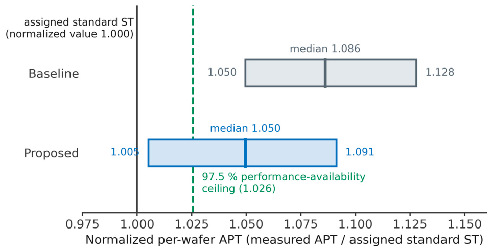
References
- Orji, N.G.; Badaroglu, M.; Barnes, B.M.; Beitia, C.; Bunday, B.D.; Celano, U.; Kline, R.J.; Neisser, M.; Obeng, Y.; Vladar, A.E. Metrology for the next generation of semiconductor devices. Nat. Electron. 2018, 1, 532–547. [Google Scholar] [CrossRef] [Scilit]
- Cooper, D.W. Particulate contamination and microelectronics manufacturing: An introduction. Aerosol Sci. Technol. 1986, 5, 287–299. [Google Scholar] [CrossRef] [Scilit]
- Born, M.; Wolf, E. Principles of Optics: Electromagnetic Theory of Propagation, Interference and Diffraction of Light, 7th ed.; Cambridge University Press: Cambridge, UK, 1999; ISBN 9780521642224. [Google Scholar]
- Smith, W.J. Modern Optical Engineering: The Design of Optical Systems, 4th ed.; McGraw-Hill: New York, NY, USA, 2007; ISBN 9780071476874. [Google Scholar]
- Kingman, J.F.C. The single server queue in heavy traffic. Math. Proc. Camb. Philos. Soc. 1961, 57, 902–904. [Google Scholar] [CrossRef] [Scilit]
- Hopp, W.J.; Spearman, M.L. Factory Physics, 3rd ed.; Waveland Press: Long Grove, IL, USA, 2011; ISBN 9781577667391. [Google Scholar]
- Little, J.D.C. A proof for the queuing formula: L = λW. Oper. Res. 1961, 9, 383–387. [Google Scholar] [CrossRef] [Scilit]
- Wein, L.M. Scheduling semiconductor wafer fabrication. IEEE Trans. Semicond. Manuf. 1988, 1, 115–130. [Google Scholar] [CrossRef] [Scilit]
- Lu, S.C.H.; Ramaswamy, D.; Kumar, P.R. Efficient scheduling policies to reduce mean and variance of cycle-time in semiconductor manufacturing plants. IEEE Trans. Semicond. Manuf. 1994, 7, 374–388. [Google Scholar] [CrossRef]
- Uzsoy, R.; Lee, C.-Y.; Martin-Vega, L.A. A review of production planning and scheduling models in the semiconductor industry part I: System characteristics, performance evaluation and production planning. IIE Trans. 1992, 24, 47–60. [Google Scholar] [CrossRef] [Scilit]
- Mönch, L.; Fowler, J.W.; Mason, S.J. Production Planning and Control for Semiconductor Wafer Fabrication Facilities: Modeling, Analysis, and Systems; Springer: New York, NY, USA, 2013. [Google Scholar] [CrossRef] [Scilit]
- Shin, H.; Shin, D. Simulation-assisted image analysis for high-sensitivity detection of 30 nm particles in non-patterned wafer inspection systems. Photonics 2026, 13, 673. [Google Scholar] [CrossRef] [Scilit]
- Greivenkamp, J.E. Field Guide to Geometrical Optics; SPIE Press: Bellingham, WA, USA, 2004. [Google Scholar] [CrossRef] [Scilit]
- Nakajima, S. Introduction to TPM: Total Productive Maintenance; Productivity Press: Cambridge, MA, USA, 1988. [Google Scholar]
- Muchiri, P.; Pintelon, L. Performance measurement using overall equipment effectiveness (OEE): Literature review and practical application discussion. Int. J. Prod. Res. 2008, 46, 3517–3535. [Google Scholar] [CrossRef] [Scilit]
- Stover, J.C. Optical Scattering: Measurement and Analysis, 3rd ed.; SPIE Press: Bellingham, WA, USA, 2012. [Google Scholar] [CrossRef] [Scilit]
- Taubenblatt, M.A.; Batchelder, J.S. Patterned wafer inspection using spatial filtering for the cluster environment. Appl. Opt. 1992, 31, 3354–3362. [Google Scholar] [CrossRef] [Scilit]
- Dom, B.E.; Brecher, V. Recent advances in the automatic inspection of integrated circuits for pattern defects. Mach. Vis. Appl. 1995, 8, 5–19. [Google Scholar] [CrossRef] [Scilit]
- Khalaj, B.H.; Aghajan, H.K.; Kailath, T. Patterned wafer inspection by high resolution spectral estimation techniques. Mach. Vis. Appl. 1994, 7, 178–185. [Google Scholar] [CrossRef] [Scilit]
- Uhrich, C.; Hesselink, L. Submicrometer defect detection in periodic structures by photorefractive holography: System design and performance. Appl. Opt. 1994, 33, 744–757. [Google Scholar] [CrossRef] [Scilit]
- Germer, T.A. Angular dependence and polarization of out-of-plane optical scattering from particulate contamination, subsurface defects, and surface microroughness. Appl. Opt. 1997, 36, 8798–8805. [Google Scholar] [CrossRef] [Scilit]
- Kim, J.H.; Ehrman, S.H.; Mulholland, G.W.; Germer, T.A. Polarized light scattering by dielectric and metallic spheres on silicon wafers. Appl. Opt. 2002, 41, 5405–5412. [Google Scholar] [CrossRef] [Scilit]
- Eremin, Y.; Orlov, N. Simulation of light scattering from a particle upon a wafer surface. Appl. Opt. 1996, 35, 6599–6604. [Google Scholar] [CrossRef] [Scilit]
- Wong, H.-S.; Yao, Y.L.; Schlig, E.S. TDI charge-coupled devices: Design and applications. IBM J. Res. Dev. 1992, 36, 83–106. [Google Scholar] [CrossRef] [Scilit]
- Lepage, G.; Bogaerts, J.; Meynants, G. Time-delay-integration architectures in CMOS image sensors. IEEE Trans. Electron Devices 2009, 56, 2524–2533. [Google Scholar] [CrossRef] [Scilit]
- Liu, C.; Xu, S.; Liu, Y.; Xiao, Z. Aperture design for a dark-field wafer defect inspection system. Appl. Opt. 2021, 60, 10830–10837. [Google Scholar] [CrossRef] [Scilit]
- Ciddor, P.E. Refractive index of air: New equations for the visible and near infrared. Appl. Opt. 1996, 35, 1566–1573. [Google Scholar] [CrossRef] [Scilit]
- Birch, K.P.; Downs, M.J. An updated Edlén equation for the refractive index of air. Metrologia 1993, 30, 155–162. [Google Scholar] [CrossRef] [Scilit]
- Yang, T.; Li, Y.; Stantchev, R.; Zhu, Y.; Qin, Y.; Zhou, X.; Huang, W. Detection of defects on the surface of a semiconductor by terahertz surface plasmon polaritons. Appl. Opt. 2016, 55, 4139–4144. [Google Scholar] [CrossRef] [Scilit]
- Chen, P.-C.; Miao, W.-C.; Ahmed, T.; Pan, Y.-Y.; Lin, C.-L.; Chen, S.-C.; Kuo, H.-C.; Tsui, B.-Y.; Lien, D.-H. Defect inspection techniques in SiC. Nanoscale Res. Lett. 2022, 17, 30. [Google Scholar] [CrossRef] [Scilit]
- Ren, Z.; Fang, F.; Yan, N.; Wu, Y. State of the art in defect detection based on machine vision. Int. J. Precis. Eng. Manuf.-Green Technol. 2022, 9, 661–691. [Google Scholar] [CrossRef] [Scilit]
- López de la Rosa, F.; Sánchez-Reolid, R.; Gómez-Sirvent, J.L.; Morales, R.; Fernández-Caballero, A. A review on machine and deep learning for semiconductor defect classification in scanning electron microscope images. Appl. Sci. 2021, 11, 9508. [Google Scholar] [CrossRef] [Scilit]
- Huang, S.-H.; Pan, Y.-C. Automated visual inspection in the semiconductor industry: A survey. Comput. Ind. 2015, 66, 1–10. [Google Scholar] [CrossRef] [Scilit]
- Chien, C.-F.; Nguyen, T.H.V.; Li, Y.-C.; Chen, Y.-J. Bayesian decision analysis for optimizing in-line metrology and defect inspection strategy for sustainable semiconductor manufacturing and an empirical study. Comput. Ind. Eng. 2023, 182, 109421. [Google Scholar] [CrossRef] [Scilit]
- Shankar, N.G.; Zhong, Z.W. Defect detection on semiconductor wafer surfaces. Microelectron. Eng. 2005, 77, 337–346. [Google Scholar] [CrossRef] [Scilit]
- Moyne, J.; Iskandar, J. Big data analytics for smart manufacturing: Case studies in semiconductor manufacturing. Processes 2017, 5, 39. [Google Scholar] [CrossRef] [Scilit]
- Chien, C.-F.; Hsu, C.-Y.; Chen, P.-N. Semiconductor fault detection and classification for yield enhancement and manufacturing intelligence. Flex. Serv. Manuf. J. 2013, 25, 367–388. [Google Scholar] [CrossRef] [Scilit]
- Jardine, A.K.S.; Lin, D.; Banjevic, D. A review on machinery diagnostics and prognostics implementing condition-based maintenance. Mech. Syst. Signal Process. 2006, 20, 1483–1510. [Google Scholar] [CrossRef] [Scilit]
- Miyazaki, Y.; Tanaka, H.; Kosaka, N.; Tomoda, T. Surface defect inspection system with an optical spatial frequency filter for semiconductor patterned wafers. Proc. SPIE 1992, 1673, 515–525. [Google Scholar] [CrossRef] [Scilit]
- Susto, G.A.; Schirru, A.; Pampuri, S.; McLoone, S.; Beghi, A. Machine learning for predictive maintenance: A multiple classifier approach. IEEE Trans. Ind. Inform. 2015, 11, 812–820. [Google Scholar] [CrossRef] [Scilit]
- Wang, C.-H. Recognition of semiconductor defect patterns using spatial filtering and spectral clustering. Expert Syst. Appl. 2008, 34, 1914–1923. [Google Scholar] [CrossRef] [Scilit]
- Schlosser, T.; Friedrich, M.; Beuth, F.; Kowerko, D. Improving automated visual fault inspection for semiconductor manufacturing using a hybrid multistage system of deep neural networks. J. Intell. Manuf. 2022, 33, 1099–1123. [Google Scholar] [CrossRef] [Scilit]
- Park, Y.-J.; Fan, S.-K.S.; Hsu, C.-Y. A review on fault detection and process diagnostics in industrial processes. Processes 2020, 8, 1123. [Google Scholar] [CrossRef] [Scilit]
- Yin, S.; Ding, S.X.; Xie, X.; Luo, H. A review on basic data-driven approaches for industrial process monitoring. IEEE Trans. Ind. Electron. 2014, 61, 6418–6428. [Google Scholar] [CrossRef] [Scilit]
- Qin, S.J. Statistical process monitoring: Basics and beyond. J. Chemom. 2003, 17, 480–502. [Google Scholar] [CrossRef] [Scilit]
- Chiang, L.H.; Russell, E.L.; Braatz, R.D. Fault Detection and Diagnosis in Industrial Systems; Springer: London, UK, 2001; ISBN 9781852333278. [Google Scholar]
- Schuirmann, D.J. A comparison of the two one-sided tests procedure and the power approach for assessing the equivalence of average bioavailability. J. Pharmacokinet. Biopharm. 1987, 15, 657–680. [Google Scholar] [CrossRef] [Scilit]
- Lakens, D. Equivalence tests: A practical primer for t tests, correlations, and meta-analyses. Soc. Psychol. Personal. Sci. 2017, 8, 355–362. [Google Scholar] [CrossRef] [Scilit]
- Yu, F.; Xu, M.; Wang, J.; Zhang, X.; Tang, X. Balancing the efficiency and sensitivity of defect inspection of non-patterned wafers with TDI-based dark-field scattering microscopy. Sensors 2024, 24, 1622. [Google Scholar] [CrossRef] [Scilit]
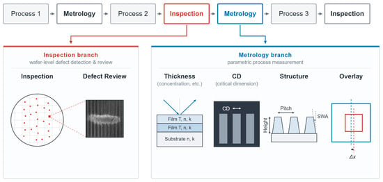
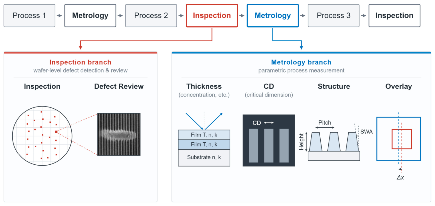
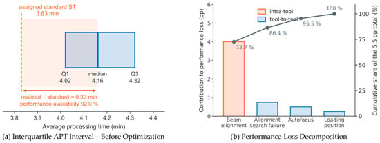
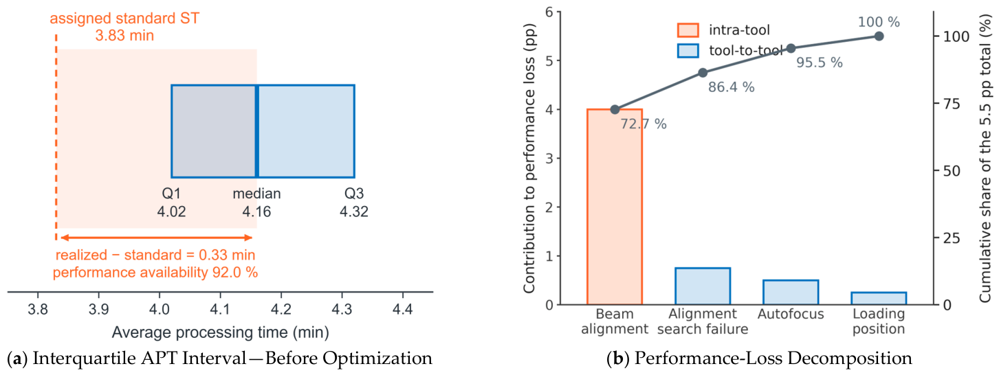
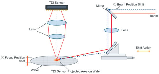
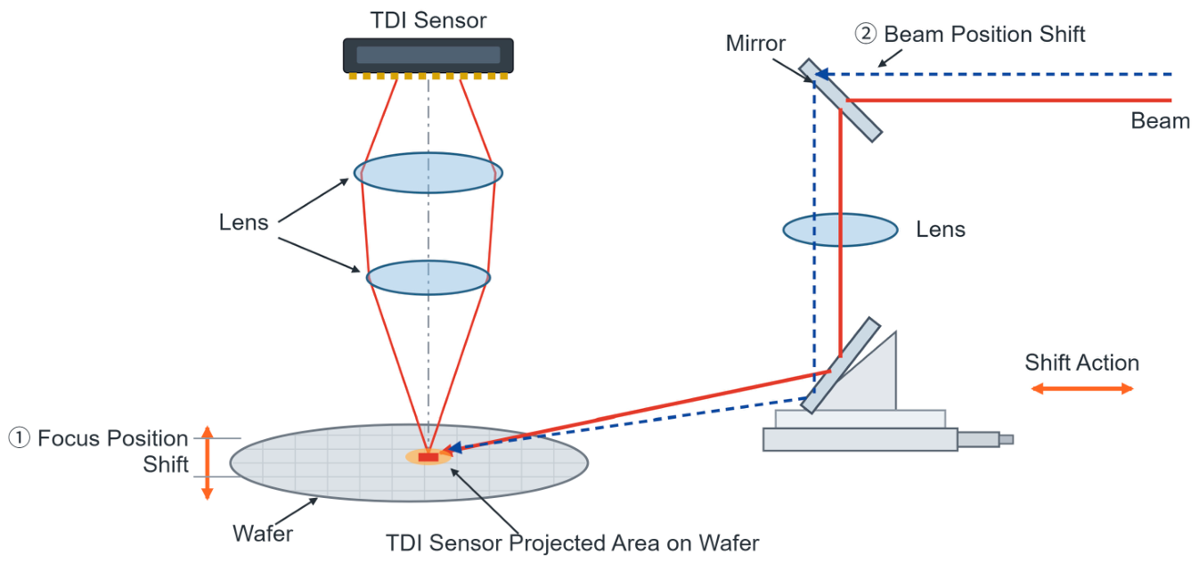
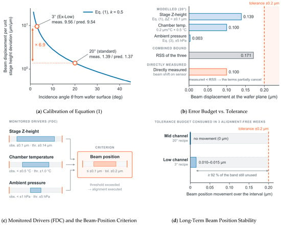
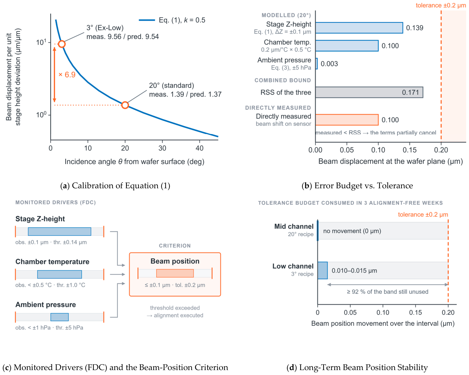
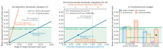
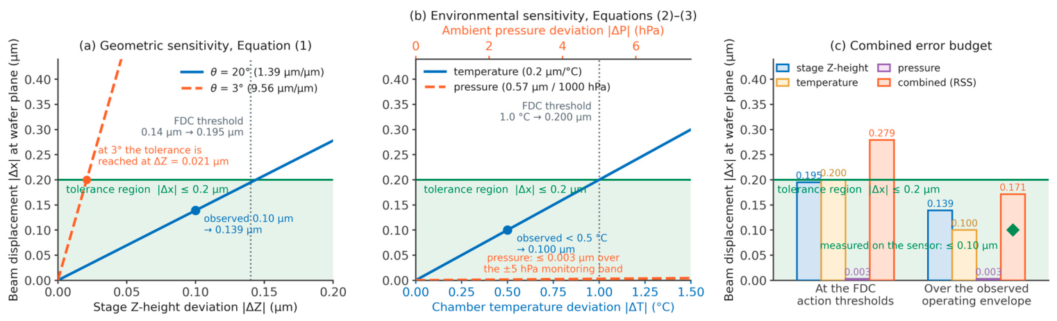
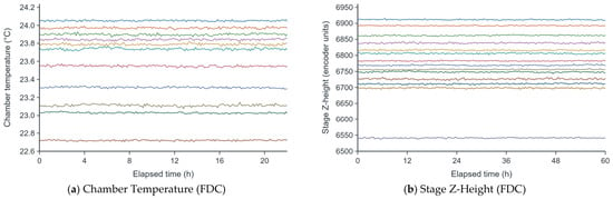
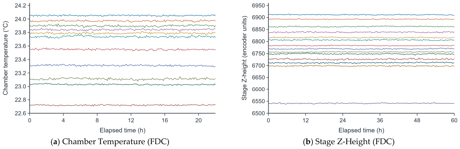
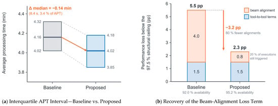
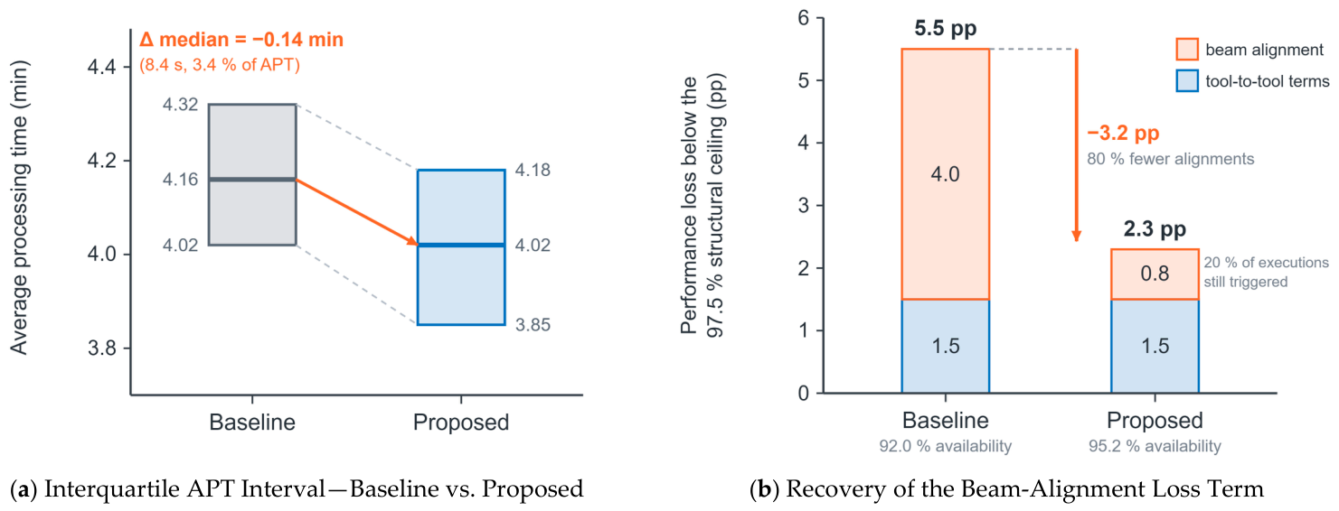

Disclaimer/Publisher’s Note: The statements, opinions and data contained in all publications are solely those of the individual author(s) and contributor(s) and not of MDPI and/or the editor(s). MDPI and/or the editor(s) disclaim responsibility for any injury to people or property resulting from any ideas, methods, instructions or products referred to in the content. |
© 2026 by the authors. Licensee MDPI, Basel, Switzerland. This article is an open access article distributed under the terms and conditions of the Creative Commons Attribution (CC BY) license.