


Abstract
Light-emitting diode (LED) sources for high-end display and professional lighting must maintain color-point accuracy and color-rendering stability over a wide correlated color temperature (CCT) range. Three-color mixing places the color point on the Planckian locus, but non-synchronous thermal drift of the channels induces CCT shift, instability, and color-rendering degradation during long-term operation. This paper proposes a green–azure–warm-white (GAW) mixing and temperature-compensation method based on the hybrid genetic–particle swarm optimization (HGPSO) algorithm. For each channel, three-Gaussian chromaticity–temperature and spectral-power-distribution–temperature models are established, and the Duv tolerance is converted into per-channel duty-cycle bounds that shrink the HGPSO search space, enabling lookup-table-based real-time compensation on an embedded MCU. Within the 30–90 °C solder-pad range, compensation reduced the average CCT deviation at 65 °C and 85 °C from 115 K and 199 K to 14.3 K and 15.8 K and the average || from 0.00167 and 0.0023 to within 0.001. The average deviation fell from 0.58% and 1.28% to 0.44% and 0.51% and the average deviation from 1.83% and 2.69% to 0.27% and 0.32%. The luminous-efficacy deviation remains within ±5% below 4500 K (maximum −8.05% at 6500 K). Cross-vendor validation confirms the portability of the method for long-term color consistency in display and lighting systems.
1. Introduction
In recent years, LEDs have gradually replaced traditional light sources and become the mainstream light source in the display and lighting field, owing to their notable advantages of compact size, low energy consumption, and long lifetime. High-end display backlights, museum lighting, professional film lighting, and medical lighting impose dual requirements on the light source: achieving wide-range CCT tunability while maintaining high color-point stability during color tuning. A single-CCT LED source can no longer meet such demands [1,2,3,4,5]. Consequently, tunable-CCT LED systems have attracted considerable attention from both academia and industry owing to their excellent adaptability and control flexibility [6,7].
To realize high-quality tunable-CCT sources, existing technical solutions mainly revolve around two approaches: dual-CCT dimming and multicolor mixing; however, the problems of color-point stability and temperature adaptability remain fundamentally unresolved [8,9,10,11]. The current mainstream scheme mostly employs two white LEDs of different CCTs for dimming-based color mixing. Although this method can achieve continuous CCT tuning within the 2700–6500 K range, the chromaticity-coordinate line connecting the two white LEDs does not coincide with the Planckian locus on the CIE 1931 chromaticity diagram. Consequently, the mixed source’s color point is distributed along the two-point connecting line rather than along the locus, leading to noticeable chromaticity-coordinate deviation in the intermediate-CCT region and reducing color-rendering accuracy; this deviation is further aggravated at elevated temperatures. To address the issue of color-point deviation from the Planckian locus, researchers have proposed three-color LED mixing schemes that adjust the luminous-flux ratio of the three channels so that the mixed source’s color point is strictly distributed along the Planckian locus, thereby ensuring chromaticity accuracy across the full CCT range. However, because the three participating LEDs employ different phosphor excitation characteristics and excitation schemes, their sensitivities to ambient temperature variation differ, causing the system to face two prominent problems under temperature fluctuation. First, chromaticity-coordinate shift causes CCT and instability. Temperature variation leads to non-synchronous drift of the three-channel chromaticity coordinates, causing the mixed color point to deviate from the Planckian locus, consequently inducing shifts in both CCT and . In practical applications, such shifts bring severe engineering consequences: in high-end lighting venues, multiple luminaires exhibit different color-point shift directions and magnitudes owing to individual thermal characteristics, destroying the overall spatial color consistency; meanwhile, inconsistent positive/negative shift directions cause the source appearance to appear greenish or purplish, and even if single-lamp metrics are acceptable, the overall spatial color performance becomes noticeably chaotic when multiple lamps are placed together. Furthermore, high-end applications such as medical lighting and professional film lighting impose strict standards on CCT and (e.g., ANSI C78.377 specifies a tolerance of no more than ±0.006, and some medical scenarios require || < 0.0005); chromaticity-coordinate shift will directly cause products to exceed the standard tolerance, failing to meet application requirements [12,13,14]. Second, spectral power distribution distortion causes color-rendering degradation. Temperature rise not only causes redshift of each channel’s spectral peak and reduction in radiation intensity, but also, owing to the significant differences in temperature sensitivity among different phosphors, the three-channel spectra exhibit different variation magnitudes and characteristics, distorting the originally optimized mixed spectral shape and ultimately causing color-rendering indicators such as the color fidelity index () and the color gamut index (Rg) to degrade significantly with temperature fluctuation, failing to guarantee long-term color stability [15,16]. In summary, although three-color LED mixing systems can achieve precise color-point control along the Planckian locus at room temperature, chromaticity-coordinate shift and spectral distortion under actual operating temperature fluctuation severely constrain their engineering application, urgently requiring a method and algorithm capable of real-time compensation of chromaticity-coordinate shift and stabilization of the spectral power distribution.
For the temperature-compensation problem of three-color LED mixing systems, existing studies have begun exploration but still exhibit obvious inadequacy in compensation dimension and precision. Some temperature-compensation methods targeting LED remain at the luminance level, restoring the output luminance to its initial state by adjusting voltage or current, without correcting the chromaticity-coordinate shift [17,18]. Liu et al. further optimized the color performance of RGBW LEDs on the basis of luminance compensation, improving the consistency of the color-rendering index [19]; however, their method suffers from high computational complexity, making real-time control on embedded platforms difficult. Meanwhile, the color-evaluation metrics employed are not comprehensive: only CCT is considered, while is neglected. Owing to metamerism, may differ significantly under the same CCT, and compensating only the CCT cannot guarantee the true accuracy of the color point. Very recently, temperature compensation for RGBW LEDs has also been investigated for automotive interior lighting [20], and the conditions for achieving thermally stable color characteristics of trichromatic, white-LED sources have been systematically analyzed [21].
Substantial progress has also been reported on tunable-CCT and multicolor LED mixing systems. Zhan et al. approximated the blackbody locus with a limited set of phosphor-converted LEDs and achieved high color fidelity across the tunable range [11]; neural-network-based controllers were later introduced to hold the target color point under time-varying ambient-light conditions [22], and bidirectional deep-learning frameworks have recently been explored for the chromatic–optical prediction and inverse design of LED systems [23]; Eissfeldt et al. proposed a virtual-channel construction that reduces a five-channel system to four independently controllable variables, enabling real-time color mixing on embedded hardware [10]. Despite this progress, three dimensions remain open. First, regarding the temperature-modeling dimension, thermal effects are either disregarded or corrected only at the luminance level [17,18,19]; the spectra of the individual channels are not predicted by an explicit SPD–temperature model, so the spectral distortion under thermal drift cannot be compensated. Second, regarding the optimization objectives, most studies optimize CCT accuracy and color rendering only, while the tolerance and the luminous-efficacy loss are seldom imposed as explicit constraints during the search. Third, regarding the hardware implementation, the optimization is usually performed offline, and the optimization results are rarely deployed as a real-time compensation strategy on a low-cost embedded controller.
As the later analysis relies on an explicit spectral description of each mixing channel, it is also worth briefly noting how LED emission is commonly modeled. Four representations are frequently employed: direct interpolation of measured SPDs, single- or double-Gaussian approximations, multi-Gaussian superpositions combining the chip emission with the phosphor band, and coupled electro-thermal–optical models [24,25,26,27]. In this work, a three-Gaussian SPD–temperature model is adopted, since the spectra of the phosphor-converted LEDs used here exhibit asymmetric multi-peak structures that single- or double-Gaussian forms cannot reproduce, while the three-Gaussian form remains analytically tractable for repeated chromaticity and color-rendering evaluations inside the optimization loop; the model formulation and its fitting accuracies (R2 > 0.985 for the chromaticity–temperature model and R2 > 0.987 for the SPD–temperature model) are detailed in Section 2.
Given the above limitations, multi-primary LED mixing to achieve tunable CCT is considered a more promising technical approach in display and lighting systems. Recent studies have further pursued this direction: evolutionary multi-objective algorithms such as NSGA-II have been applied to the spectral optimization of multi-primary phosphor-free LEDs [28]; multi-objective genetic algorithms have been employed to design four-primary-color display systems [29]; wide-gamut four-primary micro-LED architectures have likewise been demonstrated [30]; and the broader color-conversion display technology has been systematically reviewed in [31]. This scheme must not only achieve continuous CCT tuning but also jointly optimize multiple key indicators including CCT deviation, , chromaticity coordinates, and color-rendering performance, constituting a typical multi-objective optimization problem. For such complex optimization tasks with conflicting objectives, the hybrid genetic–particle swarm optimization (HGPSO) algorithm exhibits significant advantages: by fusing the local-search capability of particle swarm optimization (PSO) with the global-optimization characteristics of the genetic algorithm (GA) in a parallel architecture, HGPSO can rapidly converge to a near-optimal solution in a high-dimensional parameter space and effectively avoid the tendency of a single algorithm to fall into local optima [32,33,34,35]. The primary novelty of this work therefore lies not in the HGPSO algorithm itself—which is an established hybrid optimization framework—but in its problem-specific formulation and system-level integration for LED color mixing: (i) a chromaticity-constrained search-space reduction method that converts the tolerance into explicit per-channel duty-cycle bounds, shrinking the candidate space by more than three orders of magnitude; (ii) a three-Gaussian SPD–temperature model that enables temperature-predictive fitness evaluation; and (iii) an embedded LUT-based compensation architecture that makes the optimization results deployable in real time on a low-cost MCU. To quantify the benefit of this formulation, Section 3.3 reports a controlled benchmark in which HGPSO is compared with standard PSO and the GA under identical LED data, chromaticity constraints, population size, and stopping criteria, in both the constrained and the full (unconstrained) search spaces. However, applying HGPSO to multi-primary LED mixing still faces two major challenges: first, the increase in the number of multi-primary LED channels raises the search-space dimension, significantly increasing the computational complexity and making real-time execution on embedded systems difficult; second, spectral drift caused by temperature variation requires the mixing parameters to be dynamically adjusted with temperature, and without an accurate temperature-spectrum model, the compensation accuracy drops sharply. Therefore, reducing the algorithmic complexity through rational LED selection and temperature modeling and implementing real-time temperature compensation on an embedded platform are the keys to translating multi-primary LED mixing technology into engineering practice. To address the above challenges, this study proposes a GAW three-color LED mixing optimization and temperature-compensation method based on HGPSO. Targeting the color-point drift and color-rendering degradation problems under multi-luminaire placement and long-term continuous operation in high-end display and lighting scenarios, this method compresses the search-space dimension through GAW three-color LED selection while ensuring gamut coverage, achieves accurate characterization of each channel’s spectral variation with temperature by combining a three-Gaussian temperature-spectrum model, employs the HGPSO algorithm to solve the optimal mixing parameters under multi-objective constraints, and finally constructs a temperature-compensation LUT on an embedded platform, achieving synchronous stabilization of the color point and color-rendering performance over a wide temperature range; meanwhile, by introducing a luminous-efficacy penalty term into the fitness function to constrain luminous efficacy loss, the engineering practicality of the proposed method is ensured, providing a systematic solution for the color stability of multi-primary LED mixing systems in engineering practice.
2. Method and Experiment
2.1. Light Source Evaluation
In the CIE 1931 color space, the closed curve formed by connecting the chromaticity coordinates of monochromatic spectral colors is termed the spectral locus, which exhibits a horseshoe-shaped distribution. The region enclosed by the spectral locus and the line joining its two endpoints encompasses all physically realizable colors. An important property of the CIE x–y chromaticity diagram is that for any two chromaticity-coordinate points, all colors on the line segment joining them can be realized by spectral mixing in the corresponding proportions; if three or more chromaticity-coordinate points are selected, all colors within their convex hull can be mixed [27,36].
The chromaticity of white light is typically characterized by the CCT, defined as the temperature at which the chromaticity of a blackbody radiator matches that of the light source [37]. Based on Planck’s radiation law and the colorimetric transformation formulae, the tristimulus values and corresponding chromaticity coordinates of blackbody radiation at different temperatures can be computed. Connecting these coordinate points yields a continuous curve on the chromaticity diagram known as the Planckian locus (or blackbody locus). However, the chromaticity coordinates of a real source may deviate from the Planckian locus; in this case, the correlated color temperature is used, defined as the temperature corresponding to the point on the Planckian locus closest to the source chromaticity. For an ideal white-light source, the chromaticity coordinates should vary strictly along the Planckian locus during CCT adjustment.
To quantify the degree of deviation of a source’s chromaticity point from the Planckian locus, the parameter is introduced, which describes both the distance and the direction of the deviation of the test source’s chromaticity coordinates from the Planckian blackbody locus. An excessively large || indicates that the light color of the source deviates too far, producing a perceptually yellowish or off-color appearance [38]. is calculated as:
where are the CIE 1960 UCS chromaticity coordinates of the test source, and (u0, v0) are the CIE 1960 UCS chromaticity coordinates of the closest point on the Planckian locus to . The CIE 1960 UCS chromaticity coordinates can be converted from the chromaticity coordinates in the CIE x–y chromaticity diagram via the following relations:
To quantitatively assess the object color rendition capability of a light source, this study employs two key metrics established by the Illuminating Engineering Society (IES): color fidelity index () and color gamut index [39,40,41]. During the optimization of mixed-light sources, besides achieving the target correlated color temperature and minimizing chromaticity point deviations, it is crucial to simultaneously optimize the and parameters to ensure optimal lighting quality. The is calculated by determining the color differences between the CAM 02-UCS coordinates of each color evaluation sample (CES) under the test light source and those under a reference light source. The arithmetic mean of these color differences is then computed. represents the color similarity between the test light source and the reference light source, providing an accurate measure of average color fidelity [42,43]. When approaches 100, it indicates minimal color shifts from the reference light source, ensuring highly accurate color reproduction. In summary, during the mixed-light optimization process, achieving the target CCT and minimizing chromaticity point deviations should be complemented by optimizing and . This comprehensive approach ensures high-quality lighting with accurate color rendering and vibrant color representation.
Here, is the Euclidean distance in the CAM02-UCS color space between the test source and the reference source for the i-th color evaluation sample.
is a measure of color gamut, defined as the ratio of the area () of the polygon formed by the average coordinates in each hue-angle bin under the test source to the area () of the polygon formed by the reference illuminant:
The LED mixing performance will be evaluated from four aspects: CCT deviation, , , and . To more thoroughly investigate the effects induced by temperature variation and to seek appropriate solutions, it is necessary to establish an individual source-temperature model for each LED participating in the mixing [25,26,27]; related thermal characterization of power LEDs, including efficiency degradation and junction-temperature estimation for lifetime prediction, has been reported in [44,45].
2.2. LED Light Source Temperature Model
In terms of LED selection, to achieve white-light mixing over the 2700–6500 K CCT range (the standard tunable-CCT interval defined by ANSI C78.377, covering indoor lighting scenarios from warm to daylight [12]) with the mixed color point strictly moving along the blackbody radiation locus while ensuring good color-rendering performance and temperature stability, this study systematically evaluated candidate LED schemes from five dimensions: gamut coverage, spectral width, color rendering, control complexity, and temperature adaptability.
First, based on the chromaticity-addition principle of the CIE 1931 chromaticity diagram, the chromaticity points of the LEDs participating in the mixing must form a geometric gamut that completely encloses the target-CCT segment of the Planckian locus; this is the prerequisite for the physical realizability of the mixing [46,47,48]. Accordingly, one chromaticity point each must be selected from the green, azure, and warm-white regions to form the optimally covering large triangle. Second, to enhance the spectral continuity and color-rendering performance of the synthesized white light, the mixing LEDs should cover as wide a wavelength range as possible, thereby avoiding the insufficient caused by spectral gaps in narrowband RGB schemes. Third, given that the above two requirements are satisfied, the minimum-LED principle should be followed to reduce the search-space dimension of the HGPSO algorithm and simplify the temperature modeling and hardware-driving complexity. Considering the above, this study finally selected a green LED (G, OSRAM, peak 528.4 nm, FWHM 145.4 nm), an azure LED (A, Nichia, peak 453.0 nm, FWHM 70.2 nm), and a warm-white LED (W, OSRAM, phosphor-converted) for mixing. As shown in Figure 1, the large triangle formed by the G, A, and W chromaticity points on the CIE 1931 chromaticity diagram completely covers the 2700–6500 K segment of the Planckian locus, geometrically guaranteeing the mixability of any target chromaticity point within this CCT range. This coverage can be verified quantitatively. By the additive color-mixing principle [49], the chromaticity of any duty-cycle combination of the three channels lies within the triangle formed by the G, A, and W chromaticity points (Table 1), with the exact position determined by the mixing ratios. The Planckian locus was therefore evaluated in the CIE 1976 u′v′ diagram at 50 K intervals over 2700–6500 K: all sampled points lie strictly inside this triangle, with a minimum distance to the gamut boundary of 0.9 × 10⁻³ at 6500 K, where the locus comes closest to the A–W mixing line; the margin at the 2700 K end is 7.0 × 10⁻³. Feasibility under the imposed duty-cycle and power constraints follows from the LUT solutions: over all CCT setpoints and the full 30–90 °C range, the required duty cycles remain within the allowed range; the warm-white channel operates at its full duty of 1.0 as the base channel, while the azure and green channels remain below 0.66 and 0.03, respectively. The corresponding total electrical power stays below 0.35 W, about 24% of the summed rated channel power (1.4 W), and the required duty ratios vary continuously between setpoints, so every intermediate CCT is equally realizable. Since the temperature-induced primary shifts are corrected by the LUT compensation, the coverage is maintained over the entire operating temperature range. Meanwhile, the wide FWHM of the G channel effectively fills the green spectral gap between the blue peak of the A channel and the yellow peak of the W channel, and the phosphor-converted broadband of the W channel provides a continuous energy distribution over the 400–700 nm range. The superposition of the three yields a continuous spectrum without significant gaps, providing the spectral foundation for achieving high color-rendering performance. The relative spectral power distribution of the selected GAW LEDs together with the photopic luminous efficiency function V(λ) is shown in Figure 2.
Figure 1.
Comparison of color gamut coverage for GAW, RGB, and WW-CW configurations on the CIE 1931 chromaticity diagram.
Table 1.
Related optical parameters of GAW LED.
Figure 2.
Spectral characteristics of GAW tri-color LEDs and the photopic luminous efficiency function V(λ).
It should be noted that all LEDs used in this work were taken from the same manufacturing batch to ensure batch-level consistency. Before the formal measurements, each LED was burned in under rated current for 3 h, and measurements were performed only after the optical output had reached a stable operating state, so that the rapid initial depreciation stage of the LED lifetime curve was excluded. Each test condition was measured several times, and the reported data are statistical averages; the measurement repeatability was better than the magnitude of the temperature-induced variations under investigation. Within this framework, the spectral variations captured by the temperature models are dominated by the thermal effect, while slow aging-induced depreciation remains negligible over the test period.
During the testing process, all LEDs were driven by constant current to ensure they operate under their rated conditions. Figure 3 shows the structural block diagram of the test system, which includes an MCU driving the three LED light sources. It is important to note that changes in the junction temperature of the LEDs can cause spectral shifts, specifically manifested as peak wavelength shifts and variations in spectral intensity. To study and analyze these effects, after applying the rated current to each LED, we measure the temperature (T) of the solder pads on the LED board using temperature sensors. In this way, for each individual LED participating in the mixing, the chromaticity coordinates and the SPDs were measured at seven solder-pad temperatures from 30 °C to 90 °C, and the chromaticity–temperature and SPD–temperature models presented in the following subsections were calibrated channel by channel from these measured data.
Figure 3.
Test circuit: (a) test circuit schematic diagram; (b) main control and drive circuit; (c) LED test substrate; (d) temperature sensor.
All spectral measurements were performed with a HAAS-1200 array spectroradiometer (manufacturer: Hangzhou Everfine Photoelectric Information Co., Ltd., Hangzhou, China, China brand EVERFINE; model: HAAS-1200), covering the 380–1000 nm spectral range with a spectral resolution (FWHM) of 3.0 nm and a wavelength accuracy of ±0.3 nm. The optical head was coupled via a 1.2 m optical fiber to a 0.5 m diameter integrating sphere (Everfine), with the module mounted on the side port of the sphere in a 2π geometry, and each recorded spectrum was averaged over 10 scans. Wavelength calibration was performed with a low-pressure mercury (Hg–Ar) lamp, and radiometric calibration was performed against an EVERFINE luminous-flux/spectral radiant-flux standard lamp (e.g., SLD204, 2856 K) traceable to the National Institute of Metrology of China (NIM); the resulting calibration uncertainty, combined with the measurement repeatability (k = 1), constitutes the error bars reported in Section 3.1. The luminous efficacy reported in Section 3.2 was determined from the measured SPD: the photopic luminous flux was obtained by weighting the measured SPD with the CIE V(λ) function, and the luminous efficacy was computed as the photopically weighted flux divided by the time-averaged electrical input power of the module, measured with an EVERFINE PF9811 intelligent digital power meter.
All temperatures reported in this work refer to the solder-pad temperature measured on the LED board. The junction temperature, which fundamentally governs the spectral shift, is related to the solder-pad temperature by
where is the electrical power of each channel, and is the junction-to-solder-pad thermal resistance specified in the manufacturer datasheets. Since all LEDs were driven at constant rated current, the power dissipation is constant, and the junction-to-pad temperature difference is a fixed offset. Consequently, the solder-pad temperature and the junction temperature are in one-to-one correspondence, and the established temperature models remain physically valid with a constant temperature-axis offset that is implicitly absorbed during model fitting. The solder-pad temperature was measured using YET-620 L with an accuracy of ±(0.3%|t| + 0.40) °C, attached with thermally conductive adhesive to the copper pad approximately 0.5 mm from the LED solder joint; the sensors were calibrated against a standard before the experiments, and the overall measurement uncertainty, combining sensor accuracy, placement, and acquisition error, was estimated to be ±1 °C. The solder-pad temperature was adopted as the model variable because it can be directly and reliably measured both in the laboratory setup and in the final embedded system, whereas the junction temperature can only be estimated indirectly.
The specific parameters of the GAW LED used at 30 °C are shown in Table 1.
To visually demonstrate the chromaticity coordinate shifts of LEDs under different junction temperatures, mathematical models were developed for both the chromaticity coordinate shift trajectories and the luminance shift magnitudes. The chromaticity coordinate shift trajectories are illustrated in Figure 4; separate fitting equations were established for the chromaticity coordinates (x, y) and the luminance Y, as shown in the following formulas:
Figure 4.
Chromaticity coordinate distribution of GAW LEDs at different temperatures: (a) green LED, (b) azure LED, and (c) white LED.
The fitting mathematical equations for the chromaticity coordinates (x, y) and luminous intensity Y of the three types of LEDs are shown in Equations (8)–(11).
To verify the validity of the established mathematical model, the chromaticity coordinates of the GAW LEDs at 65 °C and 85 °C were computed using the model and compared with the actually measured chromaticity coordinates of the three LEDs at those temperatures. The results show that the measured and computed results are in close agreement, with goodness of fit R2 greater than 0.985. At 65 °C, the average shifts of the x and y coordinates of the three LEDs are 0.0007 and 0.0005, respectively; at 85 °C, the average shifts of the x and y coordinates are 0.0009 and 0.0004, respectively.
Figure 5 also allows the thermal behavior of the individual channels to be quantified. For each channel, the peak wavelength λpeak and the FWHM were extracted from the measured SPDs at each solder-pad temperature, and the corresponding luminance variation is described by the fitted models in Equation (10). Over the 30–90 °C range, the peak wavelength of the G channel shifts from 528.4 nm at a rate of 0.011 nm/°C, with the FWHM changing at 0.077 nm/°C and the luminance decreasing by 30.6%; the azure channel exhibits a peak shift from 453.0 nm at 0.022 nm/°C, a FWHM variation of 0.055 nm/°C, and a luminance decrease of 9.6%; for the W channel, the blue peak shifts at 0.015 nm/°C, the phosphor-emission band (which dominates the luminance) shifts at 0.033 nm/°C, and the luminance decreases by 6.6%, reflecting the thermal quenching of the phosphor. Among the three channels, the G channel contributes most strongly to the observed color-point drift because it suffers the strongest luminance quenching and the fastest spectral broadening, so the resulting change in spectral shape displaces its chromaticity point the most. This channel-wise imbalance in the thermal behavior is precisely why individual chromaticity–temperature and SPD–temperature models, rather than a shared model, are established for the three channels in the following subsections. In addition, because elevated temperatures induce significant shifts in the LED SPD, such as the redshift of the blue characteristic peak and the thermal quenching of the broadband phosphor emission (as illustrated in Figure 5), a mathematical model relating the absolute SPD to temperature must be established for precise analysis. Given that the SPD of the source is not a conventional single- or double-peak spectrum but rather a multi-peak composite structure formed by the superposition of a narrowband blue LED chip and a broadband phosphor emission spectrum, traditional single- or double-Gaussian models cannot accurately describe its asymmetry and shoulder characteristics. To this end, a three-Gaussian model was adopted to analytically fit the mixed spectrum [27], with the fitting formula as follows:
where S(λ) is the absolute spectral power distribution, A represents the integral area under the curve, ω is a custom width parameter, and is the peak wavelength.
Figure 5.
The spectral power distribution of GAW LEDs at different temperatures: (a) green LED, (b) azure LED, and (c) white LED.
Based on the above model, the SPDs of the green, azure, and white LEDs were fitted individually. The three-Gaussian parameters in Equation (11) were estimated for each LED by the Levenberg–Marquardt nonlinear least-squares method. The initial peak wavelength was set to the wavelength of the maximum radiant intensity in the measured spectrum, the initial width to the measured FWHM, and the initial integrated area was obtained by trapezoidal numerical integration of the measured spectrum. The fitting converged when the relative change in the residual sum of squares was below or after at most 300 iterations, and the coefficient of determination R2 was computed for each fitted spectrum. The fitting results at 30 °C are shown in Figure 6.
Figure 6.
Displays the measured spectra and fitted spectra of LEDs at 30 ◦C for (a) green LED, (b) azure LED, and (c) white LED.
Based on the fitted models, the SPD of each LED can be described by three characteristic parameters: the peak intensity, the peak wavelength, and the FWHM. Each of the nine fitted parameters (A1, A2, A3, , , , , and ) was expressed as a quadratic polynomial in the temperature T, so that an SPD function with temperature as the independent variable can be constructed. The resulting coefficient matrices for the green, azure, and white LEDs are given in Equations (14)–(16).
The selection of polynomial order is the result of a trade-off between flexibility and robustness. Since the chromaticity shift of the fluorescence conversion channel is nonlinearly affected by temperature, the first-order model shows a systematic residual trend and cannot reproduce the measured curvature. For the chromatic coordinates and SPD parameters, a third-order and second-order polynomial are, respectively, used for fitting, which can reduce the fitting residuals to a level comparable to the measurement repeatability. The high-order polynomials are intentionally discarded because the number of temperature samples measured is limited, and the number of coefficients of the high-order polynomials is close to the number of samples, resulting in regression degradation to interpolation, fitting measurement noise, and severe oscillations between temperature nodes, which instead reduces the prediction accuracy in the intermediate temperature range.
To verify the reliability of the model, the computed SPDs were compared with the measured SPDs. The matching between the measured and model-computed SPDs of the three LEDs at 30 °C, 45 °C, 65 °C, and 85 °C was compared, and the corresponding coefficients of determination are recorded in Table 2. The results show that the model-computed results agree well with the measured SPDs, with an greater than 0.987.
Table 2.
Spectral fitting coefficients for GAW LEDs sources at different temperatures.
The adopted model reproduced the measured spectra with a normalized RMSE below 4% of the peak across all fitting temperatures, and the hold-out validation at 50 °C yielded a comparable NRMSE of 3.1%, confirming the predictive rather than merely descriptive accuracy of the model.
2.3. HGPSO and Chromaticity Coordinate Limits
The HGPSO algorithm is commonly used to solve complex multi-objective optimization problems. The problem to be solved in this study is how to ensure that, as the CCT and temperature vary, the chromaticity point of the mixed source moves strictly along the Planckian locus while maintaining optimal color-rendering performance. The CCT and were used as the criteria for judging whether the source chromaticity point satisfies the requirements, while and were used as the criteria for evaluating the color-rendering capability. The multi-band LEDs were mixed using pulse-width modulation (PWM); the SPD of the combined source is a linear combination of the individual SPDs, and the duty cycles of the three LED channels were taken as the three dimensions determining the spatial position of each particle.
Here, are the duty cycles of the respective LEDs, and represent the absolute SPDs of the white, azure, and green LEDs.
One of the goals of mixed-light design is to make the chromaticity coordinates of the synthesized white light as close as possible to the blackbody locus. Based on this goal, the search space of the algorithm can be constrained to improve computational efficiency. Before executing the algorithm, the established chromaticity–temperature model can be used to predict the chromaticity coordinate shifts of LEDs at different temperatures. It is important to note that since the chromaticity coordinates of light sources do not have linear superposition properties, the principle of tristimulus value superposition must be used to calculate the chromaticity coordinates of the mixed light source at different temperatures.
We define the tristimulus values for the green LED, azure LED, and white LED as , , and , respectively, when they participate in the mixing. The tristimulus values of the mixed light source are . The relationship between them is as follows:
Additionally, based on the blackbody locus, we calculate the target white-light chromaticity coordinates and determine the x and y limits that satisfy . Taking 2700 K white light as an example, the CIE 1960 UCS chromaticity coordinates for 2700 K white light are (0.2625, 0.3516). After calculation, the determined chromaticity coordinate range that satisfies the condition is x ∈ (0.45, 0.4702) and y ∈ (0.4001, 0.4216).
After determining the target CCT point and its tolerance range, the ranges of the luminance values satisfying the constraints can be obtained for any CCT condition. The specific constraint relations are as follows:
Based on the constraints, the ranges of the luminance , , and of each channel satisfying the conditions can be computed. The duty cycle of each channel is defined as the ratio of the mixing luminance to the rated maximum luminance, yielding the constrained range of the duty cycle of each channel, which effectively shrinks the search space and significantly improves the computational efficiency. However, owing to the limitation of chromaticity matching imposed by metamerism, satisfying the duty-cycle constraint can only ensure that the mixed source meets the chromaticity-tolerance requirement, without simultaneously guaranteeing other spectral-performance indices. Therefore, it is necessary to continue searching within this interval for the optimal result satisfying all the optimization objectives.
Here, and are the maximum luminance values of the three LEDs under rated power.
According to Formulas (20) and (21), at the given CCT and temperature, the feasible duty-cycle intervals for the three channels only occupy a small portion of the entire space. When the duty-cycle resolution is 0.01, the unconstrained space contains approximately 1.0 × 10⁶ candidate combinations, while the constrained space reduces the number of candidates by several orders of magnitude. Section 3.3 of this paper systematically assesses the quantitative impact of this reduction in the search space on the convergence speed and the feasibility of the solutions.
We use the duty cycles of the three-channel LEDs as the three dimensions that determine the spatial position of particles, and the duty-cycle ranges calculated previously are used as the boundaries for particle movement. The brightness (duty-cycle) step is determined by the binary gene encoding rather than by the driver resolution or the LUT size: each channel is encoded with 7 bits, giving = 128 quantization levels, i.e., a duty-cycle step of 1/128 ≈ 0.008 (approximately 0.01), and the three-channel genome comprises 21 bits, corresponding to ≈ 2.1 × discrete combinations. The LUT stores only the optimized duty values (three per temperature point), so the step length does not affect the LUT size; a 7-bit value is additionally packable within a single byte. A comparison of 6-, 7-, and 8-bit encodings quantifies the accuracy–cost compromise of this choice. On the cost side, the discrete search space grows eightfold per added bit (2.6 × → 2.1 × → 1.7 × combinations), so the fixed evaluation budget of 5 × assessments represents a decreasing fraction of the grid (19%, 2.4%, and 0.3%), making convergence progressively harder. On the accuracy side, the worst-case chromaticity error introduced by quantization scales linearly with the step: evaluated with the colorimetric model of Section 2.1 by Monte Carlo sampling around the LUT solutions (Table 3), the worst-case |Δu′v′| amounts to 1.0 × , 4.9 × , and 2.4 × for 6, 7, and 8 bits, respectively. Because HGPSO re-optimizes the chromaticity on the discrete grid, the realized accuracy is far better than this conservative bound: the optimized solutions reach || ≤ 0.0008 (Table 3), and a local grid search around the nominal solutions shows that the worst realized || over the five setpoints amounts to 52%, 38%, and 38% of the || < 0.003 tolerance for 6, 7, and 8 bits, respectively. Eight-bit encoding would bring no practical accuracy benefit at eight times the search cost, whereas six-bit encoding consumes more than half of the tolerance at the low-CCT end. The 7-bit step (≈0.01) is therefore the coarsest encoding that keeps the realized chromaticity error well within the tolerance with sufficient margin while keeping the search space small enough for reliable convergence. We begin by initializing the population, converting the duty cycles of each color LED into corresponding 7-bit binary-encoded genes. The duty-cycle information from three channels is concatenated to form a 21-bit binary encoding, which serves as the stored genetic information. Crossover and mutation operations are performed on this set of genes.
Table 3.
The best color-mixing result at 30 °C with intensities of the three channels.
The core optimization objective of this study is to achieve accurate chromaticity-coordinate compensation for the GAW three-color LED mixing system over a wide temperature range, which requires the joint optimization of four key indicators: CCT deviation, , , and . However, since the azure channel (453 nm) is far from the peak of the human-eye photopic luminous efficiency function V(λ) (555 nm), the increased proportion of the azure channel in the high-CCT region leads to a significant decrease in luminous efficacy. Optimizing only the chromaticity and color-rendering indicators while neglecting the luminous efficacy loss would compromise the engineering practicality of the proposed method. To address this issue, a luminous-efficacy penalty term is introduced on the basis of the four core indicators, enabling the algorithm to actively balance color-point accuracy against luminous efficacy loss during the search for optimal mixing parameters, yielding the following Equation (23):
where S* is the individual fitness to be minimized, CCT_ABS is the absolute deviation between the actual CCT of an individual and the target CCT, and – are weight coefficients. LE denotes the actual luminous efficacy, and LE′ denotes the luminous efficacy of the reference light source at the same CCT. and denote the design targets of the color-rendering indices, defined as the and Rg of the designed GAW mixed light at the same CCT in the nominal state (stable 30 °C, Table 4), e.g., = 71.73 at 2700 K and = 92.56 at 4500 K. The optimization therefore seeks to preserve, at any operating temperature, the color-rendering capability of the nominal spectrum rather than to reach fixed absolute thresholds; the CCT dependence of itself is a consequence of the spectral design, and adopting the nominal-state values as targets keeps Equation (23) consistent with the compensation objectives defined on the same 30 °C baseline. Since CCT, , , , and LE have different dimensions, a prior normalization is required before weighting. In Equation (23), this normalization is realized in a reference-based relative form: every term is written as a deviation from its own fixed design reference—the target CCT, the nominal-state rendering targets and , a perfectly stable color point (|| = 0), and the same-CCT reference efficacy LE′—so that all terms vanish when their targets are exactly met and grow monotonically with the violation. Statistical normalizations such as min–max or z-score were deliberately not adopted because their reference statistics (extrema, mean, or variance) depend on the evolving population and would render the fitness landscape non-stationary across iterations, whereas the reference-based deviations remain fixed and well defined throughout the search. The residual scale differences among the five deviations are absorbed by the weights –, whose determination is described next.
Table 4.
Optimal duty cycles of the G, A, and W channels as a function of temperature for the five CCT setpoints (excerpted from the compensation LUT).
The determination of the weight coefficients is performed in two steps. First, is set to 0—that is, the luminous-efficacy penalty term is temporarily excluded—and – are determined solely for the four core indicators (CCT, , , and ). The determination of – follows the principle of core-objective priority: since the core objective of this study is accurate chromaticity-coordinate compensation, CCT and should be prioritized over and . Nine CCT sampling points were selected within the 2700–6500 K range, and the HGPSO algorithm was executed under multiple weight configurations, followed by a comparative analysis of the Pareto front distributions. The results indicate that when = 0.15, = 0.10, = 0.40, and = 0.35, the Pareto front distribution is the most uniform, effectively exploring the optimal-solution boundary in the color-point accuracy direction while maintaining solution-set diversity in the color-rendering performance direction. After – were determined, the luminous-efficacy penalty term was introduced as an auxiliary constraint, and was set to 0.20; this value was determined by comparing the optimization results under different configurations and achieves an optimal balance between luminous efficacy loss and color-point accuracy. Two properties of this weight setting are worth noting. First, although the five coefficients sum to 1.20 rather than to unity, this has no effect on the optimization: the fitness is used only for ranking individuals, and multiplying S* by any positive constant shifts all fitness values uniformly without changing the ranking or the selected optimum; Σk = 1.2 merely reflects the scale at which the weights were tuned. For ease of interpretation, the equivalent normalized weights—obtained by dividing each coefficient by Σk = 1.2—are ′ = 0.125, ′ = 0.083, ′ = 0.333, ′ = 0.292, and ′ = 0.167, which sum to unity. Second, the configuration is robust to the weight settings: in a single-parameter perturbation test, each coefficient was varied by ±50% around its nominal value with the others fixed, and the resulting Pareto fronts and the final optimal solutions remained essentially unchanged, indicating that the reported performance is not an artifact of one particular weight combination. Finally, it should be emphasized that acts as a trade-off regulator rather than a remedy: it re-weights the search between color-point accuracy and luminous efficacy, but the efficacy loss in the high-CCT region originates from the spectral position of the azure channel (453 nm) relative to the V(λ) peak (555 nm) under the chromaticity constraints; therefore mitigates, but cannot eliminate, this structural loss, as quantified in Section 3.2.
The overall flow of the algorithm is as follows: After inputting the spectral data and the spectral-ratio constraint range, initialization is performed; the initial generation is sorted according to individual fitness, and the global historical best position () and the individual historical best position () are recorded. The subsequent optimization proceeds in two parallel parts: (1) each individual updates its velocity (combining the inertia term and the guidance from the individual best and the global best) and then its position; (2) the GA operations are performed, with crossover and mutation applied to low-fitness individuals. The individuals obtained from crossover and mutation are then combined with the individuals processed by the PSO operations to form a new population. The fitness is recomputed and sorted, only the original population size is retained, and and are updated. The iterative loop continues until the set number of generations is reached. The algorithm flowchart is shown in Figure 7.
Figure 7.
HGPSO flowchart.
3. Results and Discussion
3.1. Impact of Temperature on Light Source Parameters
This study established three key compensation objectives—CCT, , and color-rendering performance ( and ) compensation—to ensure optimal output parameters over the 2700–6500 K range. Although luminous efficacy is also temperature-dependent, it is primarily governed by the channel proportion determined by CCT selection rather than temperature fluctuation and can be indirectly stabilized through spectral stabilization; its discussion is therefore deferred to the engineering-practicality evaluation section. The LED state at a stable 30 °C was defined as the standard reference, with each CCT point measured repeatedly and the data in Table 3 reported as statistical averages to ensure reliability and reproducibility. Under this baseline, the HGPSO-optimized results over 2700–6500 K yielded an average CCT deviation of 10.2 K, an average || of 0.00052, ∈ [71.73, 92.56], and ∈ [99.11, 111.57], confirming high-precision CCT control and color-rendering performance at the baseline temperature.
As the temperature rises, the SPD of the LED source changes significantly; if uncompensated and mixed directly according to the initial duty-cycle results, the parameters of the mixed source will differ substantially from the initial state. To analyze this deviation, the source parameters were subsequently measured at 65 °C and 85 °C. Figure 8 presents the deviations of CCT and ||, while Figure 9 presents the deviations of and . Error bars denote the combined standard uncertainty (k = 1) obtained from 10 repeated measurements, the root-sum-square combination of the measurement repeatability, and the spectrometer calibration uncertainty; the calibration component is common to all CCT setpoints at a given temperature, while the thermal component increases from ±0.50 and ±0.60 at 30 °C to ±0.75 and ±0.85 at 85 °C. When the operating temperature rose to 65 °C, the average CCT deviation increased to 115 K (maximum 160 K), the average || was 0.00167 (maximum 0.002) with a deviation rate of 684%, the average deviation rate reached 0.58%, and the average deviation rate reached 1.83%. When the temperature further rose to 85 °C, the average CCT deviation increased to 199 K (maximum 282 K), the average || was 0.0023 (maximum 0.003), and the average and deviation rates reached 1.28% and 2.69%, respectively. The 30 °C reference values in Table 4 were likewise obtained from repeated measurements and reported as statistical averages. It is worth noting that the non-smooth appearance of the curves is dominated by the physical and optimization structure rather than by measurement scatter: on the one hand, the chromaticity constraint || < 0.003 confines the feasible duty-cycle region at each setpoint to 0.015–0.025% of the full search space so that the optimized solution is pinned to the constraint boundary, and small differences between adjacent setpoints are directly translated into the mixing spectrum; on the other hand, the narrowband azure channel (FWHM ≈ 70 nm) makes the colorimetric quantities, aggregated over the 99 TM-30 color samples, sensitive to these small spectral-shape differences. The error bars (±0.5–0.75 for and ±0.6–0.85 for ) are substantially smaller than the setpoint-to-setpoint variation, confirming that the curve profiles reflect the true temperature response of the mixed source; after compensation, the corresponding curves in Figure 10 stay close to the 30 °C reference with average deviations of only 0.44–0.51% () and 0.27–0.32% () (Table 5).
Figure 8.
CCT and changes of light sources at different temperatures: (a) CCT; (b) .
Figure 9.
and changes of light sources at different temperatures: (a) ; (b) .
Figure 10.
Color performance of LED light source after color compensation: (a) temperature 85 °C for ; (b) temperature 85 °C for ; (c) temperature 65 °C for ; (d) temperature 65 °C for .
Table 5.
Average optical parameters of the GAW source before and after temperature compensation at 65 °C and 85 °C.
Studies indicate that a || exceeding 0.001 already induces a visible greenish or purplish color-appearance shift, and at 0.003, the shift becomes distinctly perceptible [3,14]. Chromaticity tolerances differ strongly across applications: ANSI C78.377 specifies a tolerance of ±0.006 for nominal white light in general lighting [12], whereas certain color-critical medical applications are reported to require || < 0.0005 [13,14]. The uncompensated || values of 0.00167 (65 °C) and 0.0023 (85 °C) therefore remain within the ANSI C78.377 limit, but they exceed both the 0.001 visibility threshold and the 0.0005 level required by color-critical applications, which would cause perceivable color-appearance inconsistency under multi-luminaire placement. Establishing a temperature-compensation mechanism to suppress the shift is thus a necessary condition for color-point stability in professional lighting.
It should be emphasized that although the CCT deviation itself remains within an acceptable range for general lighting scenarios, the accompanying || shift has a more critical impact on practical applications. As a scalar metric, CCT reflects only the numerical change in color temperature, whereas directly characterizes the distance of the chromaticity point from the Planckian locus and is the core parameter governing human color-appearance perception.
3.2. Temperature Compensation
Due to being limited by the computational capability of the experimental MCU, the system cannot run HGPSO in real time to perform the mixing-channel ratio computation and temperature compensation. To minimize the impact of computational latency on system performance, the compensation parameters for each temperature point were precomputed from 30 °C to 90 °C in 1 °C steps and stored in the MCU, thereby constructing a LUT-based dynamic temperature-compensation mechanism that enables rapid correction of the LED output parameters according to the real-time monitored temperature.
Beyond serving as a deployment mechanism, the precomputed LUT directly documents how the optimum channel balance evolves as the spectra drift with temperature. For each temperature point on the 30–90 °C grid, the channel spectra predicted by the temperature models established in Section 2 were fed into the same HGPSO routine under the identical chromaticity constraint (|| < 0.003) and weight configuration, and the resulting optimal duty cycles were stored in the LUT. Table 4 excerpts the resulting G, A, and W channel contributions at the three experimentally characterized temperatures (30 °C, 65 °C, and 85 °C) for the five CCT setpoints of Table 3.
As shown in Table 4, the compensation is realized almost entirely by re-balancing the narrowband channels: the white channel remains at its rated maximum duty of 1 across the entire temperature range, while at 6500 K, the azure duty shifts from 0.634 at 30 °C to 0.589 at 85 °C and the green duty from 0.005 to 0.002. This continuous re-balancing is the mechanism behind the performance recovery in Table 5: because the three channels drift non-synchronously with temperature, holding the mixed color point on the Planckian locus requires the duty ratio to be re-solved at every temperature rather than fixed at its 30 °C value. The direction and magnitude of the duty adjustments are consistent with the per-channel drift behavior quantified in Section 2, confirming that the compensation operates by tracking the temperature-induced spectral drift rather than by static trimming.
It should be clarified that the real-time operation of the embedded system refers to LUT-based temperature compensation rather than to real-time execution of the HGPSO optimization: the HGPSO optimization is performed offline on a PC, and the MCU executes only temperature acquisition, LUT lookup, and PWM updating. The system is built on an STM32F103C8T6 microcontroller (ARM Cortex-M3, 72 MHz, 64 KB Flash, 20 KB SRAM). The LUT stores the precomputed duty cycles for 9 target CCTs × 61 temperature points × 3 channels at 8-bit resolution, occupying approximately 1.6 KB (1647 bytes), i.e., less than 2.6% of the on-chip Flash. On the 72 MHz core, a LUT lookup requires approximately 1 µs, and the updated duty cycle takes effect within one PWM carrier period (50 µs at the 20 kHz carrier), so the lookup-and-update latency is below 0.1 ms; the solder-pad temperature is sampled once per second, which dominates the end-to-end control latency of approximately 1 s (still two to three orders of magnitude smaller than the thermal time constants of the system). This offline optimization/online-compensation separation guarantees deterministic real-time behavior on a low-cost MCU while retaining the optimization quality of HGPSO.
The priority of the optimization objectives was set by adjusting the weighting coefficients in Equation (23), with CCT and (taken as unified characterization parameters of chromaticity-coordinate shift) compensated first, followed by and as color-rendering performance indicators. During the algorithmic screening, individuals with the minimal chromaticity-coordinate shift (CCT and closest to the set targets) were preferentially selected as the optimization solutions. After compensation, the performance of the source at 65 °C and 85 °C is shown in Figure 10 and Figure 11 and Table 5, while Figure 12 visualizes the underlying color-point restoration on the CIE 1931 chromaticity diagram.
Figure 11.
and CCT of LED light source after color compensation: (a) temperature 85 °C for ; (b) temperature 85 °C for CCT; (c) temperature 65 °C for ; (d) temperature 65 °C for CCT.
Figure 12.
Chromaticities of the 20 CCT setpoints (30, 65, and 85 °C) before and after compensation: (a) CIE 1931 overview; (b,c) magnified views of the 4500 K and 2700 K setpoints.
The detailed results are given in Table 5, where the uncompensated and compensated cases are compared directly. After temperature compensation, at 85 °C, the average CCT deviation was 15.8 K, and || was controlled within 0.001, effectively suppressing the chromaticity-coordinate shift; meanwhile, the average deviation was 0.51%, and the average deviation was 0.32%. At 65 °C, the average CCT deviation was 14.3 K, || was controlled within 0.001, the average deviation was 0.44%, and the average deviation was 0.27%.
The worst cases over the investigated CCT and temperature ranges are reported explicitly. For the uncompensated source, the maximum deviations occur at the 2700 K setpoint, reaching ΔCCT = 282 K and || = 0.003 at 85 °C, whereas the deviations in the neutral-white region (4500–5500 K) remain the smallest. After compensation, the maximum residual deviations are ΔCCT = 21 K, || = 0.0006, Δ = 1.5%, and Δ = 1%. After compensation, the maximum residual deviations relative to the 30 °C nominal state are ΔCCT = 21 K, |Duv| = 0.0006, Δ = 1.5%, and Δ = 1% at 85 °C; the CCT and Duv residuals peak near the 5000–5500 K setpoints, whereas the Rf and Rg residuals are largest at the warm-CCT end (Figure 10 and Figure 11).
This behavior is consistent with the distribution of the correction authority over the CCT range: at 2700 K, the mixed spectrum is dominated by the warm-white channel, with azure and green duties of only 0.031 and 0.015 (Table 3), so the two narrowband channels that perform the correction contribute the smallest share of the mixture; in the neutral-white region, the azure channel operates at intermediate duties (0.33–0.49), providing the largest correction authority and the smallest residual deviations. This tendency is directly visible in Figure 12a: the uncompensated points (hollow symbols) drift along the Planckian locus toward warmer CCTs and away from it in the direction, whereas the compensated points (filled symbols) cluster tightly around the target chromaticities and fall within the || = 0.003 corridor at all setpoints and temperatures. The magnified views in Figure 12b,c resolve the neutral-white region, where the correction authority is largest, and the 2700 K warm end, where the residual deviations are the largest over the investigated range yet remain inside the tolerance band. The 30 °C nominal state, which serves as the compensation reference, is reproduced identically before and after compensation.
One limitation of the GAW configuration should be stated explicitly. The color-rendering performance at 2700 K is noticeably lower than that in the neutral-white region: even at the 30 °C reference condition, before any thermal drift occurs, the optimized at 2700 K is 71.7, about 21 points lower than the 92.6 obtained at 4500 K. This gap originates from the hardware channel set rather than from the optimization or compensation framework. High-fidelity reproduction of a warm-white reference spectrum requires substantial long-wavelength energy beyond approximately 600 nm; in the GAW configuration, however, the only contribution in this region is the broadband phosphor tail of the warm-white channel, since the green (peak 528 nm) and azure (peak 453 nm) channels provide negligible emission above 600 nm and no independently addressable red or amber primary is available, so the optimizer cannot shape the long-wavelength part of the spectrum regardless of the optimization method. It should be emphasized that this limitation does not undermine the optimization or compensation scheme itself—the chromaticity accuracy at 2700 K remains within the same tolerances as at the other setpoints—but it does restrict the current three-channel implementation in warm-CCT applications with stringent color-fidelity requirements (e.g., > 90); for such applications, extending the channel set with an amber or red primary, as noted in the Conclusions, would be the appropriate engineering choice.
Furthermore, to verify that the proposed method possesses good portability and engineering practicality, this study further selected six different LED devices from three manufacturers: Honourtek, OSRAM, and Bridgelux. Two mixed light source systems were constructed for testing and validation, with specific device parameters shown in Table 6. The experiments employed the same HGPSO optimization and temperature compensation methods proposed in this paper. The performance results after compensation are illustrated in Figure 13 and Table 7.
Table 6.
Optical parameters of six different LEDs.
Figure 13.
Color performance of LED light source with 30 °C, 65 °C, and 85 °C after color compensation. (a) Combination1 for . (b) Combination1 for . (c) Combination2 LED for . (d) Combination2 LED for .
Table 7.
CCT, color-rendering, and luminous-efficacy results before and after compensation for the two cross-vendor combinations.
After compensation, the two cross-vendor combinations maintained an average CCT deviation of 9–17 K and || within 0. 001 at 65 °C and 85 °C (Table 7), while the average and deviations with respect to the 30 °C nominal state remained within 1% and 0.8%, respectively, and the compensated luminous efficacy ranged from 76 to 88 lm/W. Regarding the device models, the temperature models were not shared across devices: each of the six LEDs was individually characterized before the experiment, with the chromaticity-coordinate–temperature and SPD–temperature data measured at seven temperature points between 30 °C and 90 °C and the three-Gaussian coefficients fitted per device using the identical procedure described in Section 2; the subsequent duty-cycle bounding, HGPSO optimization, and LUT generation then ran without any manual re-tuning. The portability demonstrated here should therefore be understood as portability of the method rather than of the parameters: the model structure, optimization formulation, and compensation architecture transfer to new devices without modification, while the model coefficients are device-specific and are obtained by a one-time off-line thermal–spectral characterization, which is a standard requirement for model-based temperature compensation. The same condition applies to channel selection: a new channel set must still satisfy the gamut-coverage requirement of Section 2 for the target CCT range. The two combinations were deliberately selected to span different manufacturers and channel pairings (six devices from three manufacturers in total) so as to cover the device-level diversity encountered in practice; together with the per-device characterization of all six LEDs, they provide system-level evidence of portability, although the sample size remains limited as acknowledged in Section 4.
To comprehensively evaluate the dynamic temperature-compensation performance of the system, the source was tested in constant-temperature environments at 20 °C and 40 °C. The target CCT was set to 4000 K; starting from source turn-on, the operating-temperature variation with time was continuously monitored, and key performance parameters such as CCT, , , and were synchronously acquired. The dynamic deviation of each performance index from start-up to thermal steady state was analyzed to verify the response capability and compensation effect of the temperature-compensation algorithm under different ambient temperatures and heating rates. The result is shown in Figure 14.
Figure 14.
Temperature compensation results at dynamic temperatures: (a) 20 °C constant temperature; (b) 40 °C constant temperature.
It should be clarified that the experiments in Figure 13 are intrinsically dynamic rather than constant-temperature measurements. The LEDs were driven from a cold start at constant current, so the solder-pad temperature rose continuously from approximately 30 °C to 60 °C (20 °C ambient) and to 85 °C (40 °C ambient), while the compensation loop remained active throughout the thermal transient. The solder-pad temperature, CCT, ||, , and were sampled every 2 s, so the reported curves represent the complete dynamic trajectories rather than steady-state snapshots. The settling behavior is as follows: after start-up, the deviation increased temporarily during the rapid temperature rise, reached its maximum at approximately 4 min, and then decreased monotonically, settling within ±1% after approximately 10 min and remaining stable thereafter. A varying-temperature experiment under an externally imposed thermal ramp is beyond the scope of the present study and is noted as future work.
Because multiple source-performance indices (CCT, , , and ) are considered, to more intuitively quantify the deviation between the measured and theoretically computed performance, a deviation parameter was introduced to synthesize the multiple performance indices, computed as:
where CCT is the target correlated color temperature, the theoretical color fidelity index, the theoretical gamut index, and the theoretical chromaticity deviation; CCT′, , , and are the corresponding measured values.
The results show that over time, when operating at a 20 °C ambient temperature, the source temperature rises to approximately 60 °C and then stabilizes; the maximum optical-performance deviation was 4.9%, with an average deviation of 3.41%. At a 40 °C ambient temperature, the source temperature rises to approximately 85 °C and then stabilizes; the maximum optical-performance deviation was 5.31%, with an average deviation of 3.55%. Among them, 4.9% and 5.31% of the transient deviations can be attributed to the elimination effect. According to the performance of the MCU and the sampling rate, the lookup and update calculations are completed within 0.1 milliseconds, and the sampling interval is 1 s, both of which are one order of magnitude shorter than the involved thermal transient process. Therefore, the control loop delay cannot explain the deviations that last for several minutes. Similarly, the influence of systematic LUT or interpolation errors can be excluded because, in the steady state, this transient deviation disappears. However, both the transient and steady-state stages go through the same measurement–lookup–update chain. Therefore, the dominant factor is the mismatch in thermal inertia between the sensor and the heating structure: the sensor monitors the pad temperature (Section 2.2), which lags behind the junction temperature, with a time constant of approximately several minutes. Thus, during the preheating process, the LUT index is based on the lagging temperature, resulting in temporary insufficient compensation. The actual impact of this transient deviation is limited and predictable: the deviation exists only in the first few minutes after startup, its direction is fixed during the transient period, and it converges to the steady-state accuracy after reaching equilibrium.
To evaluate the engineering practicality of the GAW mixed source, its luminous efficacy was measured over the full 2700–6500 K range, with a commercial Bridgelux LED at the same CCT serving as the reference baseline, as shown in Figure 15 and Table 8. The luminous efficacy of the Bridgelux commercial LED increases approximately linearly with the CCT, rising from approximately 113 lm/W at 2700 K to approximately 136 lm/W at 6500 K. The luminous efficacy of the GAW source exhibits a rapid-then-slow growth trend, rising from approximately 114 lm/W at 2700 K to approximately 125.2 lm/W at 6500 K. The efficacy-deviation curve shows that in the low-CCT region (2700–3000 K), the GAW source is slightly higher than the Bridgelux LED (deviation of +0.8% to +1.38%); the two become equal at approximately 3200 K; above 3500 K, the GAW source falls below the Bridgelux LED, with the deviation increasing nonlinearly as CCT rises, reaching −8.05% at 6500 K.
Figure 15.
Luminous efficacy and relative deviation of the GAW source versus the Bridgelux LED across 2700–6500 K.
Table 8.
Luminous efficacy of the GAW source and the Bridgelux LED at 2700–6500 K.
The efficacy difference between the two sources originates from the difference in their SPD composition. The Bridgelux commercial LED employs a blue chip to excite a yellow phosphor, producing a continuous broadband spectrum with energy concentrated near the V(λ) peak (555 nm); as the blue component increases with the CCT, the luminous efficacy continues to rise. The GAW source is synthesized by mixing three channels (green at 528 nm, azure at 453 nm, and warm-white), and its luminous efficacy depends on the energy contribution of each channel under V(λ) weighting. In the low-CCT region, the warm-white channel dominates, and its spectral peak (approximately 560 nm) is close to the V(λ) peak, so the GAW source efficacy is comparable to that of the Bridgelux LED. As the CCT increases, the proportion of the azure channel rises. Since its wavelength is far from the V(λ) peak, the growth in GAW source luminous efficacy is smaller than that of the Bridgelux LED.
Despite the above efficacy loss, the GAW source retains differentiated engineering applicability across different CCT regions. In the 2700–3500 K region, the efficacy deviation is within ±2%, and the source provides a stable color point, making it suitable for applications with strict color-consistency requirements such as museum lighting and professional film lighting; it should be noted, however, that color rendering in this region is bounded by the channel configuration (ten-run mean ≈ 72 at 2700 K), so the demonstrated benefit is color-point stability rather than high color fidelity. In the 3500–5000 K region, the efficacy deviation ranges from −2.24% to −6.01%, achieving a good balance between color-point accuracy and luminous efficacy, with color-rendering indices ( ≈ 84–93) adequate for high-end commercial and medical lighting applications. In the 5000–6500 K region, the efficacy deviation reaches −6.01% to −8.05%, indicating a more pronounced efficacy loss; however, the color-point stability and the maintained color-rendering indices ( ≈ 89–93) still make the source suitable for special applications where color-consistency requirements take precedence over efficacy requirements.
Viewed jointly with the compensation results, these data quantify the Pareto trade-off actually realized by the optimization: across the full 2700–6500 K range, the chromaticity objectives were essentially fully achieved (average CCT deviations of 14.3 K at 65 °C and 15.8 K at 85 °C, with || controlled within 0.001, well inside the 0.003 design tolerance), while the efficacy position relative to the commercial baseline changes from +0.8% to +1.38% in the low-CCT region to −8.05% at 6500 K; the residual efficacy loss is thus the price paid for pinning the color point and the rendering performance. This loss is structural rather than an artifact of the weighting: under the chromaticity constraints (|| < 0.003), the admissible duty-cycle region at each CCT is narrow, and as CCT rises, the azure channel (453 nm)—far from the V(λ) peak (555 nm)—must carry a larger share of the radiant power, which bounds the attainable efficacy of the mixed spectrum itself. The luminous-efficacy penalty term operates on this structural trade-off as a regulator: with the adopted = 0.20 the realized operating point is exactly the one quantified above, and increasing can buy back efficacy only by spending the chromaticity and color-rendering margin, whereas decreasing shifts the solution in the opposite direction; it mitigates but cannot eliminate the high-CCT efficacy loss. For efficacy-sensitive applications, the weight settings can therefore be re-tuned within this trade-off, and the spectrum comparison is shown in Figure 16.
Figure 16.
Comparison of optimal spectra with phosphor-converted LEDs at two CCTs.
3.3. Computational Performance Benchmark
To quantify the computational cost of the proposed method and the reported performance, which is systematic rather than dependent on a particular random initialization, a controlled benchmark was conducted. All experiments were implemented in MATLAB R2022a and executed on an Intel Core i7–12700H CPU with 24 GB RAM. The optimizer settings were identical to those in Section 2 (population size n = 100, 500 generations, and duty-cycle resolution 0.01), so that every run performs a fixed budget of 100 × 500 = 5.0 × 10⁴ fitness evaluations. The three algorithms—HGPSO, standard PSO, and the GA—were benchmarked under identical LED data, fitness function (Equation (23)), generation budget, and initialization protocol, in both the constrained search space defined by the chromaticity-derived duty-cycle bounds (Section 2) and the full unconstrained cube [0, 1]3. The chromaticity constraint (|| < 0.003) is an engineering requirement inherited from the application rather than an algorithmic mechanism, so the constrained formulation does not privilege any particular algorithm. For each configuration, ten independent runs were performed, each with its own randomly generated initial population; within each paired cross-algorithm comparison, common random numbers were used (all algorithms were seeded with the same initial population), so that performance differences are attributable to the search mechanisms rather than to initialization. Results are reported as the mean ± standard deviation over the ten runs, together with the best and worst values.
The benefit of the constrained formulation is first quantified geometrically. Monte Carlo sampling of 2 × 10⁷ duty-cycle triples uniformly distributed in the unit cube shows that at the nominal 30 °C state, the region satisfying the chromaticity requirement (|| ≤ 0.003 with respect to the target CCT, within a ±200 K band) occupies only 0.015–0.025% of the cube across the nine setpoints (Table 9), i.e., the chromaticity-derived bounds shrink the effective search space by three to four orders of magnitude (≈4.0 × 10³ to 6.5 × 10³ per setpoint). At initialization, when the population is uniformly distributed over the cube, a population of 100 individuals therefore contains on average only ≈0.02 feasible members in the unconstrained space; the constrained formulation eliminates this waste by construction, since initialization, position updates, and boundary handling are all restricted to the chromaticity-derived interval set so that essentially the entire evaluation budget is spent on admissible candidates. Table 10 reports the algorithmic consequences at the representative 4500 K setpoint: in the unconstrained space, the first feasible solution appeared only after 186 ± 92 generations on average (versus 0 generations in the constrained space), 2 of the 10 unconstrained HGPSO runs failed to reach the chromaticity tolerance within the 500-generation budget, and the mean final fitness was 4.1 × for the unconstrained configuration versus 2.8 × for the constrained configuration.
Table 9.
Feasible fraction of the full duty-cycle space and the resulting search-space reduction at the nine CCT setpoints.
Table 10.
Computational performance of HGPSO, PSO, and the GA with and without the chromaticity-constrained search space at 4500 K (ten runs per configuration).
In terms of computational cost, a single constrained HGPSO run completes in 600 ± 14 s on the benchmark platform, while PSO and the GA require 585 ± 11 s and 592 ± 13 s under the same evaluation budget. The memory footprint of the optimizer itself is negligible: the population state (positions, velocities, and personal/global bests for N = 100 three-dimensional individuals) amounts to 8 KB. More importantly, the optimizer is executed offline; the deployed compensator does not run any search at runtime but evaluates a pre-computed duty-cycle LUT (61 temperature points ×3 channels per setpoint, i.e., 183 entries per setpoint) on the embedded MCU, whose real-time response is demonstrated in Section 3.2 (Figure 13). The convergence behavior of all configurations is shown in Figure 17, which compares the three algorithms under the identical budget in the constrained space. HGPSO reached its fitness plateau within 150 generations and exhibited no stagnation events (defined as no improvement of the best-so-far fitness for more than 50 consecutive generations) in any of the ten runs, whereas PSO stagnated in four of the ten runs, and the GA required >500 generations to reach the mean final fitness attained by HGPSO. This is consistent with the complementarity of the two coupled operators in HGPSO: the genetic crossover and mutation applied to low-fitness individuals re-inject diversity exactly where the swarm has collapsed, mitigating premature convergence, while the PSO velocity guidance accelerates exploitation around promising regions; the GA lacks the velocity guidance and therefore converges more slowly, and standard PSO lacks the regeneration mechanism and is consequently more prone to stagnation. Finally, Table 11 reports the across-run statistics of HGPSO at all nine setpoints over ten independent runs: the relative standard deviation of the final fitness remains below 5% at every setpoint, and all runs satisfy the chromaticity tolerance, confirming that the compensation performance reported in Section 3.1 (Table 4) is robust against the stochastic nature of the optimization.
Figure 17.
Convergence at 4500 K: (a) comparison of HGPSO, PSO, and GA; (b) constrained vs. unconstrained HGPSO.
Table 11.
Across-run statistics of HGPSO over ten independent runs at the nine CCT setpoints.
3.4. Comparison with Existing Studies
To close the literature loop, the differences between the present method and the main technical families reviewed above are summarized along the three dimensions introduced in Section 1, namely the temperature-modeling depth, the completeness of the optimization objectives, and the hardware-implementation level. The relevant families include luminance- or output-level temperature compensation [8,17,18], real-time color mixing without an explicit thermal model [10], color-control optimization for high color rendering [11], neural-network-based color control [22], and optimization-based RGBW temperature compensation [19].
Regarding the temperature-modeling dimension, the luminance- and output-level schemes correct the thermal drift after it appears at the output, whereas the RGBW method in [19] adjusts the mixing ratios on the basis of output consistency; in contrast, the present method establishes an explicit three-Gaussian SPD–temperature model for every participating channel so that the spectral change of each channel is predicted rather than corrected afterwards. Regarding the optimization objectives, earlier studies typically target CCT accuracy and color-rendering indices, while the tolerance and the luminous-efficacy loss are seldom imposed as explicit constraints; in the present work, the fitness function (Equation (23)) jointly includes the deviation, the deviation, the CCT deviation, ||, and the luminous-efficacy penalty, and the chromaticity constraint || < 0.003 is imposed throughout the search. Regarding the hardware implementation, real-time color mixing has been demonstrated on embedded platforms [13], but without thermal compensation; the present work instead follows an offline-optimization/online-compensation architecture: HGPSO is executed once offline (Section 3.3), and the resulting duty-cycle LUTs are deployed on a low-cost embedded MCU, where the real-time temperature compensation is performed (Figure 13).
To clarify the positioning of the proposed method relative to the state of the art, the studies closest in purpose to this work are compared qualitatively here. The junction-temperature-feedback schemes [8,17,18] compensate only the luminous output and leave the temperature-induced chromaticity shift uncorrected. The RGBW method [19] extends the compensation to color-rendering indices but at a computational cost that is difficult to accommodate on embedded platforms, and it evaluates the color point through CCT alone without considering . The multi-channel mixing systems [10] achieve color tuning over a range of CCTs but do not explicitly compensate for temperature-induced drift, and the recent stability analysis of trichromatic sources in [21] establishes the conditions under which the color point can be kept thermally stable but does not address color-rendering metrics or embedded implementation. Very recently, temperature compensation for RGBW LEDs has been investigated for automotive interior lighting [20], evolutionary multi-objective algorithms have been applied to the spectral optimization of multi-primary LEDs [28] and four-primary display systems [29], and bidirectional deep learning frameworks have been explored for chromatic–optical prediction and inverse design [23]. Compared with these efforts, the proposed GAW scheme differs in three respects: it jointly compensates CCT, ||, , and rather than a subset of these quantities; it covers a 30–90 °C solder-pad temperature range through a per-temperature LUT that executes in real time on a low-cost MCU; and its effectiveness is verified experimentally across the full 2700–6500 K CCT range and across devices from three manufacturers.
In summary, the comparison indicates that the contribution of this work lies not in a new optimization algorithm but in a problem-specific integration that jointly closes the three gaps identified above: an analytically constrained search space with a reduction of more than three orders of magnitude (Section 3.3), a spectral-level temperature model embedded in the fitness evaluation, and a deployable LUT compensation architecture for real-time embedded operation.
4. Conclusions
To address the degradation of color consistency caused by temperature variations over a wide CCT range in applications such as display backlights, museum lighting, and professional film lighting, this paper proposes a GAW three-color LED mixing-optimization and temperature-compensation method based on an HGPSO algorithm. The GAW channels—comprising a green LED, an azure LED, and a phosphor-converted warm-white LED—were systematically selected based on five dimensions: gamut coverage, spectral width, color rendering, control complexity, and temperature adaptability. This selection ensures that the CIE 1931 gamut triangle fully encloses the 2700–6500 K Planckian segment while maintaining a continuous synthesized spectrum. For each channel, chromaticity-coordinate–temperature and spectral-power-distribution–temperature models were established. The HGPSO search space was constrained by || < 0.003, and a LUT approach was adopted to enable real-time temperature compensation on an embedded MCU, thereby achieving an effective balance between algorithmic efficiency and compensation accuracy. It should be noted that the demonstrated benefit of the compensation is color-point stability over temperature; color rendering at very warm CCTs remains bounded by the three-channel configuration (Section 3.2).
Experimental results demonstrate that without compensation, raising the solder-pad temperature from 30 °C to 85 °C causes the average CCT deviation to increase from 10.2 K to 199 K and the average || from 0.00052 to 0.0023, exceeding the 0.001 threshold of visible color-appearance shift. Following the implementation of the proposed compensation scheme, within the solder-pad temperature range of 30–90 °C, the GAW mixed light source maintained high chromaticity stability across the 2700–6500 K range. The compensation accuracy is not uniform across the CCT range: the method performs best in the neutral-white region (approximately 4500–5500 K), where the residual deviations remain close to the 30 °C reference level, whereas the largest residual deviations occur at the boundary setpoints of the range, in particular at 2700 K (Section 3.2). At 65 °C, the average CCT deviation was 14.3 K, the average deviation was 0.44%, and the average deviation was 0.27%. At 85 °C, the average CCT deviation was 15.8 K, the average deviation was 0.51%, and the average deviation was 0.32%, with | consistently controlled within 0.001. Across the nine setpoints of Table 11, the ten-run mean ranges from 71.7 at 2700 K to 92.9 at 5000 K, and the ten-run mean from 98.7 at 6500 K to 111.8 at 2700 K. In absolute terms at the average level, the compensated source achieved = 86.3 and = 103.4 at 65 °C and = 86.2 and = 103.4 at 85 °C against 30 °C reference values of = 86.7 and = 103.7.
The GAW source exhibits luminous efficacy comparable to commercial phosphor-converted white LEDs (pc-LEDs) in the low-CCT region. However, a decline in efficacy is observed in the high-CCT region. This is attributed to the increased proportion of the azure channel, whose peak wavelength deviates from the V(λ) maximum. Specifically, below 4500 K, the relative efficacy deviation of the GAW source remains within ±5%, which is acceptable for practical engineering applications. Above 4500 K, this deviation gradually increases with CCT, reaching approximately −8.05% at 6500 K. Dynamic-compensation experiments further indicate that the average optical-performance deviations at ambient temperatures of 20 °C and 40 °C were maintained within 3.41% and 3.55%, respectively.
Cross-vendor validation using two additional LED combinations confirms that following compensation, the CCT deviation remained below 20 K, || was controlled within 0.001, and the average color-rendering deviations remained within 1% () and 0.8% (). These results demonstrate the portability of the proposed workflow and architecture across manufacturers: after the required one-time per-device thermal–spectral characterization, the same modeling, optimization, and compensation procedure can be applied without modification. This portability of the methodology does not imply independence from the LED type or manufacturer: each device must still be characterized individually, and the achievable performance depends on the specific channel spectra.
The principal contribution of this study lies in providing a comprehensive engineering and technical solution for display and lighting systems, encompassing LED selection, temperature modeling, algorithmic optimization, and real-time compensation, thereby providing a practical technical reference for color-consistency assurance in high-end display backlights and professional lighting applications. The limitations of this study are as follows: the temperature-modeling range is confined to 30–90 °C and does not encompass extreme low-temperature (<0 °C) or high-temperature (>100 °C) scenarios; the compensation accuracy of the LUT method is bounded by the 1 °C temperature-sampling step; the color-rendering capability at very warm CCTs is bounded by the three-channel configuration (ten-run mean ≈ 72 at 2700 K), so high-fidelity warm-white operation would require an additional amber or red primary; and although data from three manufacturers were incorporated, the sample size remains limited. Moreover, this study targets the reversible spectral drift caused by junction-temperature variation within normal operating conditions; the long-term irreversible thermal-aging degradation (e.g., phosphor deterioration and package yellowing) is beyond its scope. Since the compensation is implemented as duty-cycle LUTs, slow aging drifts can, in principle, be absorbed by periodically re-calibrating the LUTs, which will be investigated in future work. Future work may explore modeling over a wider temperature range, neural-network-based real-time compensation algorithms, and the extension of the proposed method to RGBW, RGBA, and other multi-primary LED systems.
Author Contributions
Z.X.: Conceptualization, data curation, software, formal analysis, investigation, methodology, validation, writing—original draft, and writing—review and editing. Z.L.: Conceptualization, methodology, visualization, writing—original draft, and writing—review and editing. C.Z.: Resources and supervision. M.H.: Resources. Z.Z.: Funding acquisition, project administration, and supervision. All authors have read and agreed to the published version of the manuscript.
Funding
This study was funded by the National Natural Science Foundation of China (62475077, 62135003); the Natural Science Foundation of Guangdong Province (2024A1515010586); the Special Project for Research and Development in Key areas of Guangdong Province (2022B0303040003); the Guangzhou Municipal Science and Technology Project (202201010704); the Guangdong Special Support Plan (2023TY07Z039); and the Horizontal Project of Shenzhen CNHT Co., Ltd. (342387).
Data Availability Statement
Data will be made available on request.
Acknowledgments
This work was also supported by grants from the Guangdong Special Support Plan (Grant No. 2023TY07Z039) and the Horizontal Project of Shenzhen CNHT Co., Ltd. (Grant No. 342387). The authors would like to thank the editors and reviewers for their valuable comments that helped us improve this manuscript.
Conflicts of Interest
Author Chaohui Zhuang was employed by the company Company of Shenzhen Rayconn Electronics. The remaining authors declare that the research was conducted in the absence of any commercial or financial relationships that could be construed as a potential conflict of interest.
References
- Hayashida, T.; Iwasaki, H.; Masaoka, K.; Shimizu, M.; Yamashita, T.; Iwai, W. Appropriate indices for color rendition and their recommended values for UHDTV production using white LED lighting. Opt. Express 2017, 25, 15010–15027. [Google Scholar] [CrossRef] [Scilit] [PubMed]
- Qiao, L.; Zhang, H.; Yu, J.; Cao, F.; Gao, Y. Design of smart light source based on bi-color LED with single duty cycle for correlated color temperature adjustment. Opt. Quantum Electron. 2021, 53, 610. [Google Scholar] [CrossRef] [Scilit]
- Neyezhmakov, P.; Pitiakov, O.; Shpak, S.; Kyslytsia, S.; Kozhushko, G. The current state of energy efficiency and light quality of led products. Ukr. Metrol. J. 2022, 1, 12–19. [Google Scholar] [CrossRef] [Scilit]
- Huang, Z.; Chen, W.; Liu, Q.; Wang, Y.; Pointer, M.R.; Liu, Y.; Liang, J. Towards an optimum colour preference metric for white light sources: A comprehensive investigation based on empirical data. Opt. Express 2021, 29, 6302–6319. [Google Scholar] [CrossRef] [Scilit] [PubMed]
- Yang, W.; Jeon, J.Y. Effects of correlated colour temperature of LED light on visual sensation, perception, and cognitive performance in a classroom lighting environment. Sustainability 2020, 12, 4051. [Google Scholar] [CrossRef] [Scilit]
- Oh, J.H.; Yang, S.J.; Do, Y.R. Healthy, natural, efficient and tunable lighting: Four-package white LEDs for optimizing the circadian effect, color quality and vision performance. Light Sci. Appl. 2014, 3, e141. [Google Scholar] [CrossRef] [Scilit]
- Zhang, M.; Chen, Y.; He, G. Color Temperature Tunable White-Light LED Cluster with Extrahigh Color Rendering Index. Sci. World J. 2014, 2014, 897960. [Google Scholar] [CrossRef] [Scilit] [PubMed]
- Qu, X.; Wong, S.C.; Chi, K.T. Temperature measurement technique for stabilizing the light output of RGB LED lamps. IEEE Trans. Instrum. Meas. 2009, 59, 661–670. [Google Scholar] [CrossRef] [Scilit]
- Zhu, L.; Yao, B.; Deng, L.; Yang, Y.; Wang, G.; Gu, C.; Xu, L. Evaluation of gamut enhancement in yellow regions and a choice of optimal wavelength for a RGBY four-primary laser display system. Opt. Express 2022, 30, 38938–38952. [Google Scholar] [CrossRef] [Scilit] [PubMed]
- Eissfeldt, A.; Khanh, T.Q. Algorithm for real-time colour mixing of a five-channel LED system while optimising spectral quality parameters. Light. Res. Technol. 2022, 54, 563–575. [Google Scholar] [CrossRef] [Scilit]
- Zhan, X.; Wang, W.; Chung, H.S.H. A novel color control method for multicolor LED systems to achieve high color rendering indexes. IEEE Trans. Power Electron. 2017, 33, 8246–8258. [Google Scholar] [CrossRef] [Scilit]
- ANSI C78.377-2017; American National Standard for Electric Lamps—Specifications for the Chromaticity of Solid State Lighting Products. American National Standards Institute: Washington, DC, USA, 2017. Available online: https://www.nema.org/standards/view/American-National-Standard-for-Electric-Lamps (accessed on 8 July 2026).
- Durmus, D. Correlated color temperature: Use and limitations. Light. Res. Technol. 2022, 54, 363–375. [Google Scholar] [CrossRef] [Scilit]
- Royer, M.; Murdoch, M.J.; Smet, K.; Whitehead, L.; David, A.; Houser, K.; Esposito, T.; Livingston, J.; Ohno, Y. Improved Method for Evaluating and Specifying the Chromaticity of Light Sources. Leukos 2023, 19, 35–52. [Google Scholar] [CrossRef] [Scilit]
- Chhajed, S.; Xi, Y.; Li, Y.-L.; Gessmann, T.h.; Schubert, E.F. Influence of junction temperature on chromaticity and color-rendering properties of trichromatic white-light sources based on light-emitting diodes. J. Appl. Phys. 2005, 97, 054506. [Google Scholar] [CrossRef] [Scilit]
- van de Haar, M.A.; Tachikirt, M.; Berends, A.C.; Krames, M.R.; Meijerink, A.; Rabouw, F.T. Saturation Mechanisms in Common LED Phosphors. ACS Photonics 2021, 8, 1784–1793. [Google Scholar] [CrossRef] [Scilit] [PubMed]
- Sisto, M.; Gauvin, J. Accurate chromatic control and color rendering optimization in LED lighting systems using junction temperature feedback. In Proceedings of SPIE Optics + Photonics, Thirteenth International Conference on Solid State Lighting, San Diego, CA, USA, 17–21 August 2014; SPIE: Bellingham, WA, USA, 2014; Volume 9190. [Google Scholar] [CrossRef] [Scilit]
- Park, S.-C.; Park, K.-H.; Chang, J.-H. Luminance-Degradation Compensation Based on Multistream Self-Attention to Address Thin-Film Transistor-Organic Light Emitting Diode Burn-In. Sensors 2021, 21, 3182. [Google Scholar] [CrossRef] [Scilit] [PubMed]
- Liu, X.; Jiang, C.; Liu, X.; Liu, Z.; Hu, M.; Zhuang, Z. RGBW LED mixing temperature compensation method with high output consistency. Opt. Laser Technol. 2024, 171, 110440. [Google Scholar] [CrossRef] [Scilit]
- Rapaccini, D.; Falaschetti, L.; Lissandron, S.; Conti, M.; Orcioni, S.; Morici, A. Temperature compensation for chromatic stability of RGBW LEDs in automotive interior lighting. Electronics 2025, 14, 3451. [Google Scholar] [CrossRef] [Scilit]
- Onwukaeme, C.; Ryu, H. Conditions for thermally stable color characteristics of trichromatic white light-emitting diodes. Opt. Express 2024, 32, 44581. [Google Scholar] [CrossRef] [Scilit]
- Zhan, X.; Wang, W.; Chung, H. A neural-network-based color control method for multi-color LED systems. IEEE Trans. Power Electron. 2018, 34, 7900–7913. [Google Scholar] [CrossRef] [Scilit]
- Lin, S.; Chen, H.; Lin, Z.; Xie, Q.; Chen, C.; Lin, H.; Shen, X.; Lin, S. Bidirectional deep learning for chromatic-optical predicting and inverse design of LED systems with multi-objective optimization of circadian efficacy and gamut. Opt. Express 2025, 33, 50278. [Google Scholar] [CrossRef] [Scilit] [PubMed]
- Reifegerste, F.; Lienig, J. Modelling of the temperature and current dependence of LED spectra. J. Light Vis. Environ. 2008, 32, 288–294. [Google Scholar] [CrossRef] [Scilit]
- Ye, H.; Koh, S.W.; Yuan, C.; van Zeijl, H.; Gielen, A.W.J.; Lee, S.-W.R.; Zhang, G. Electrical–thermal–luminous–chromatic model of phosphor-converted white light-emitting diodes. Appl. Therm. Eng. 2014, 63, 588–597. [Google Scholar] [CrossRef] [Scilit]
- Cai, M.; Yang, D.; Tian, K.; Chen, W.; Chen, X.; Zhang, P.; Fan, X.; Zhang, G. A hybrid prediction method on luminous flux maintenance of high-power LED lamps. Appl. Therm. Eng. 2016, 95, 482–490. [Google Scholar] [CrossRef] [Scilit]
- Tan, Q.; Rao, F.; Xu, H.; Zhang, Y. LED spectral model characterized by several Gaussian functions. Chin. J. Opt. Appl. Opt. 2012, 5, 493–498. [Google Scholar] [CrossRef] [Scilit]
- Dang, X.; Zeng, C.; Wang, G.; Zhu, X.; Zhou, M.; Wan, Q.; Luo, L.; Guo, X.; Zhao, J.; Xiong, Z. Spectral optimization of multi-primary-color phosphor-free LEDs for healthy lighting by NSGA-II. Opt. Laser Technol. 2025, 192, 113652. [Google Scholar] [CrossRef] [Scilit]
- Ke, S.; Kuang, Q.; Lin, Y.; Ye, L.; Yang, K.; Chen, Z.; Yao, M.; Chai, Y.; Guo, Z. A four-primary-color healthy display system designed with multi-objective genetic algorithms based on user age and application scenarios. Opt. Laser Technol. 2025, 184, 112514. [Google Scholar] [CrossRef] [Scilit]
- Sun, P.; Min, M.; Wu, Q.; Huang, W.; Xiao, Q.; Xiao, W.; Zheng, C. A four-primary-color micro-LED display with wide color gamut, low blue light hazard, and promise to improve working efficiency in the working conditions. AIP Adv. 2025, 15, 015008. [Google Scholar] [CrossRef] [Scilit]
- Li, G.; Tseng, M.-C.; Chen, Y.; Yeung, F.S.-Y.; He, H.; Cheng, Y.; Cai, J.; Chen, E.; Kwok, H.-S. Color-conversion displays: Current status and future outlook. Light Sci. Appl. 2024, 13, 301. [Google Scholar] [CrossRef] [Scilit] [PubMed]
- Chen, X.; Du, W.; Qi, R.; Qian, F.; Tianfield, H. Hybrid gradient particle swarm optimization for dynamic optimization problems of chemical processes. Asia-Pac. J. Chem. Eng. 2013, 8, 708–720. [Google Scholar] [CrossRef] [Scilit]
- Shehadeh, H.A. A hybrid sperm swarm optimization and gravitational search algorithm (HSSOGSA) for global optimization. Neural Comput. Appl. 2021, 33, 11739–11752. [Google Scholar] [CrossRef] [Scilit]
- Duan, B.; Guo, C.; Liu, H. A hybrid genetic-particle swarm optimization algorithm for multi-constraint optimization problems. Soft Comput. 2022, 26, 11695–11711. [Google Scholar] [CrossRef] [Scilit]
- Lv, X.; Zhou, D.; Li, F. Test optimization selection based on HGPSO Algorithm. In Proceedings of the 7th International Conference on Control Engineering and Artificial Intelligence (CCEAI ’23), Sanya, China, 28–30 January 2023; Association for Computing Machinery: New York, NY, USA, 2023; pp. 113–117. [Google Scholar] [CrossRef] [Scilit]
- Ren, H.; Li, S.; Sun, R.; Su, Z. Study on LED color mixing for stage lighting based on locus fitting of blackbody. In 2017 International Conference on Computer Technology, Electronics and Communication (ICCTEC), Dalian, China, 19–21 December 2017; IEEE: New York, NY, USA, 2017; pp. 295–299. [Google Scholar] [CrossRef] [Scilit]
- Li, C.; Cui, G.; Melgosa, M.; Ruan, X.; Zhang, Y.; Ma, L.; Xiao, K.; Luo, M.R. Accurate method for computing correlated color temperature. Opt. Express 2016, 24, 14066–14078. [Google Scholar] [CrossRef] [Scilit] [PubMed]
- Li, C.; Luo, M.R.; Melgosa, M.; Pointer, M.R. Testing the accuracy of methods for the computation of CIE tristimulus values using weighting tables. Color Res. Appl. 2016, 41, 125–142. [Google Scholar] [CrossRef] [Scilit]
- ANSI/IES TM-30-18; IES Method for Evaluating Light Source Color Rendition. ANSI/IES: Washington, DC, USA, 2018.
- Royer, M.P. Comparing measures of average color fidelity. Leukos 2018, 14, 69–85. [Google Scholar] [CrossRef] [Scilit]
- Qu, X.; Siu, W.; Chi, T. Color Control System for RGB LED Light Sources Using Junction Temperature Measurement. In IECON 2007—33rd Annual Conference of the IEEE Industrial Electronics Society, Taipei, Taiwan, 5–8 November 2007; IECON Proceedings (Industrial Electronics Conference); IEEE: New York, NY, USA, 2007; pp. 1363–1368. [Google Scholar] [CrossRef] [Scilit]
- Balocco, C.; Volante, G. A Method for Sustainable Lighting, Preventive Conservation, Energy Design and Technology—Lighting a Historical Church Converted into a University Library. Sustainability 2019, 11, 3145. [Google Scholar] [CrossRef] [Scilit]
- Ohno, Y.; David, A.; Houser, K.; Wei, M.; Royer, M.; Smet, K.; Whitehead, L. Development of the IES method for evaluating the color rendition of light. Opt. Express 2015, 23, 15888–15906. [Google Scholar] [CrossRef] [Scilit] [PubMed]
- Plotog, I.; Vladescu, M. Power LED efficiency in relation to operating temperature. In SPIE Advanced Topics in Optoelectronics, Microelectronics, and Nanotechnologies, Constanta, Romania, 21–24 August 2014; Advanced Topics in Optoelectronics, Microelectronics, and Nanotechnologies VII; SPIE: Bellingham, WA, USA, 2015; Volume 9258, pp. 652–657. [Google Scholar] [CrossRef] [Scilit]
- Rammohan, A.; Ramesh Kumar, C.; Chandramohan, V.P. Experimental analysis on estimating junction temperature and service life of high power LED array. Microelectron. Reliab. 2021, 120, 114121. [Google Scholar] [CrossRef] [Scilit]
- Žukauskas, A.; Vaicekauskas, R.; Ivanauskas, F.; Vaitkevičius, H.; Shur, M.S. Spectral Optimization of Phosphor-Conversion Light-Emitting Diodes for Ultimate Color Rendering. Appl. Phys. Lett. 2008, 93, 051115. [Google Scholar] [CrossRef] [Scilit]
- Khanh, T.Q.; Bodrogi, P.; Vinh, T.Q. Human Centric Lighting and Color Quality. In Color Quality of Semiconductor and Conventional Light Sources; Wiley: Hoboken, NJ, USA, 2017; pp. 335–355. [Google Scholar] [CrossRef] [Scilit]
- Dangol, R.; Islam, M.S.; Hyvärinen, M.; Bhushal, P.; Puolakka, M.; Halonen, L. User acceptance studies for LED office lighting: Preference, naturalness and colourfulness. Light. Res. Technol. 2013, 47, 36–53. [Google Scholar] [CrossRef] [Scilit]
- Schubert, E.F. Light-Emitting Diodes, 2nd ed.; Cambridge University Press: Cambridge, UK, 2006. [Google Scholar] [CrossRef] [Scilit]
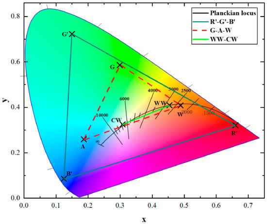
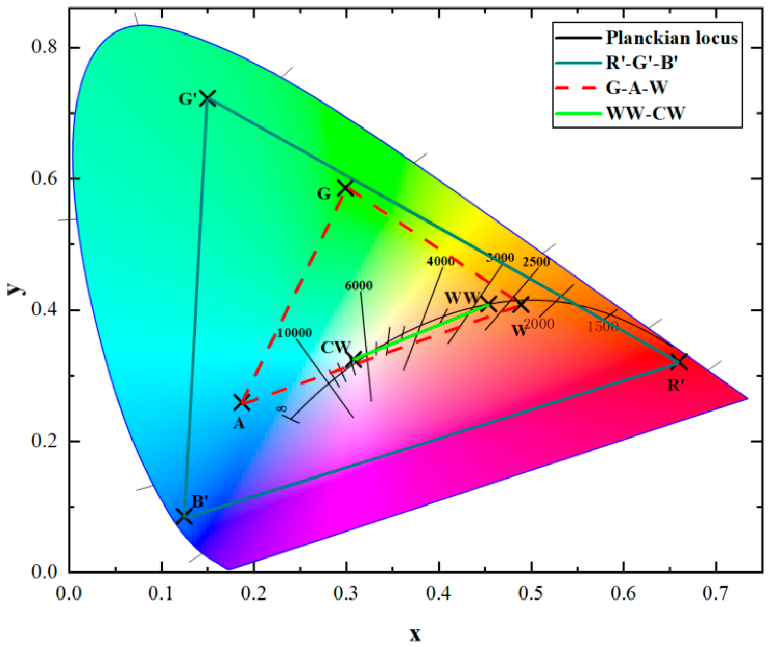
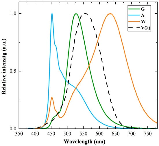
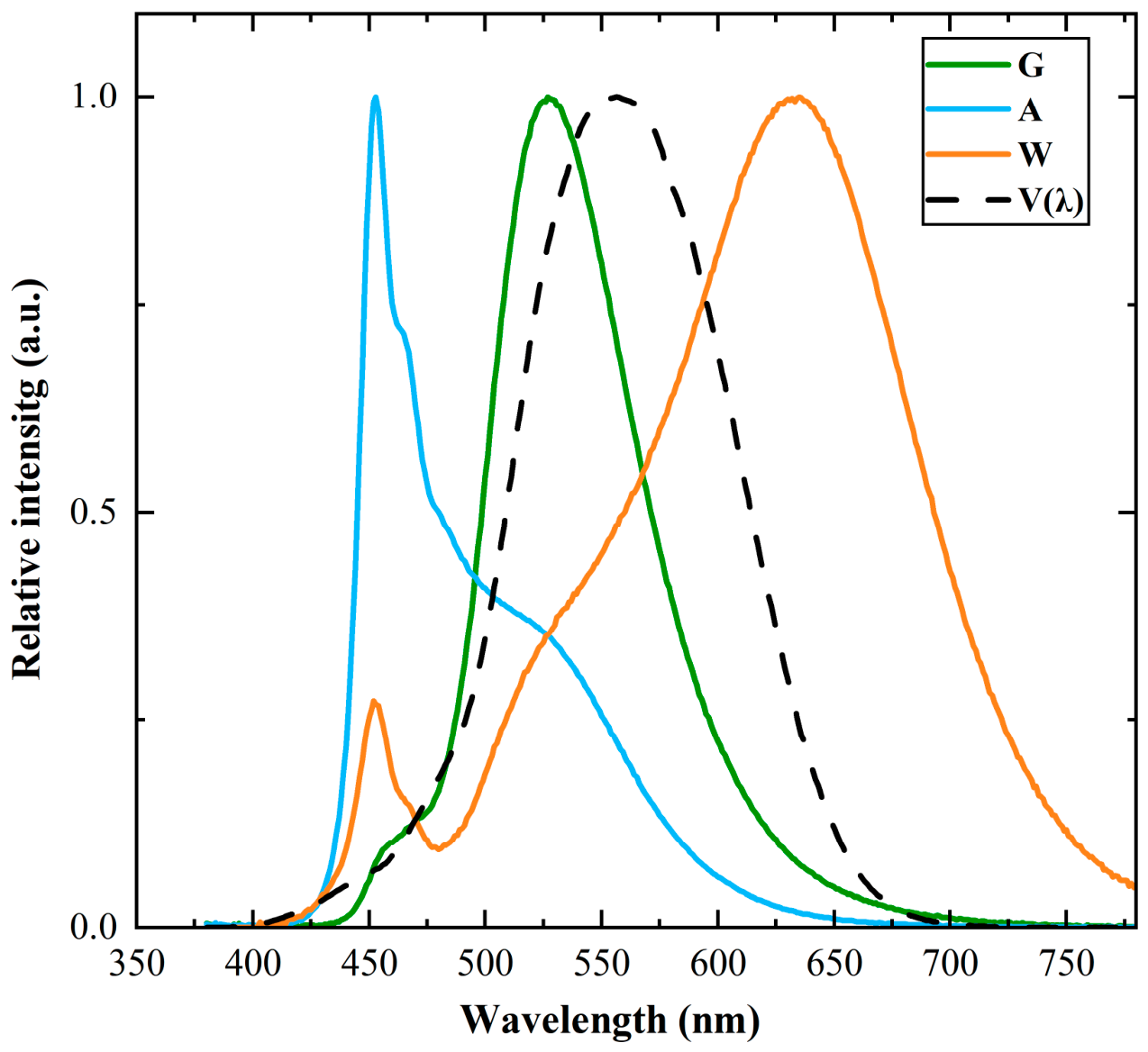
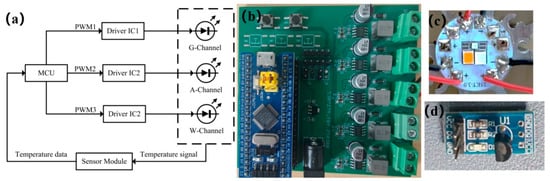
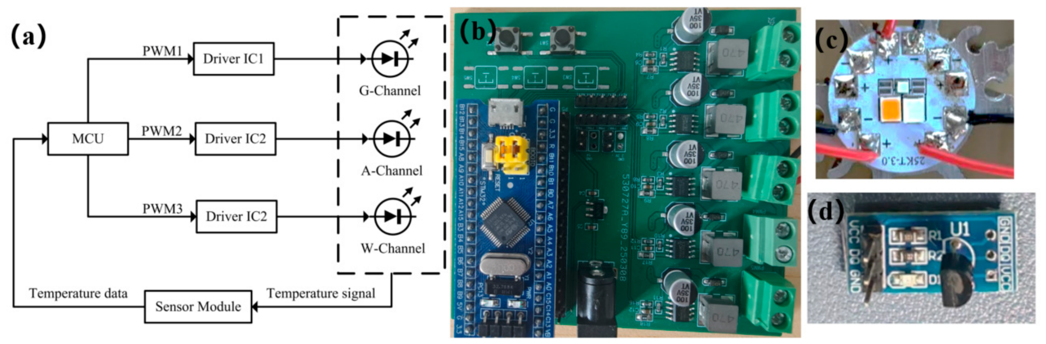
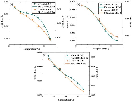
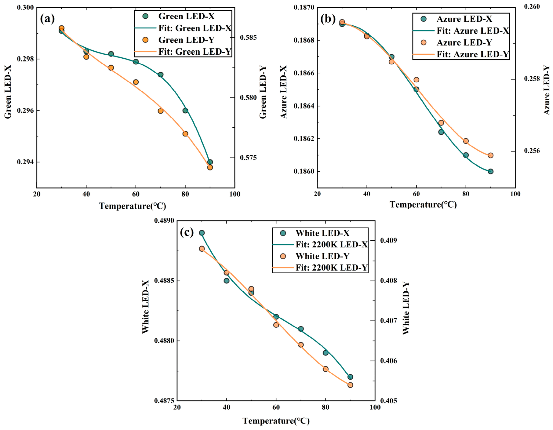
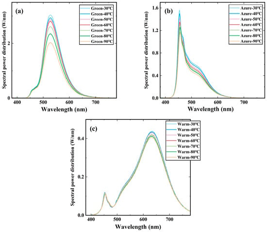
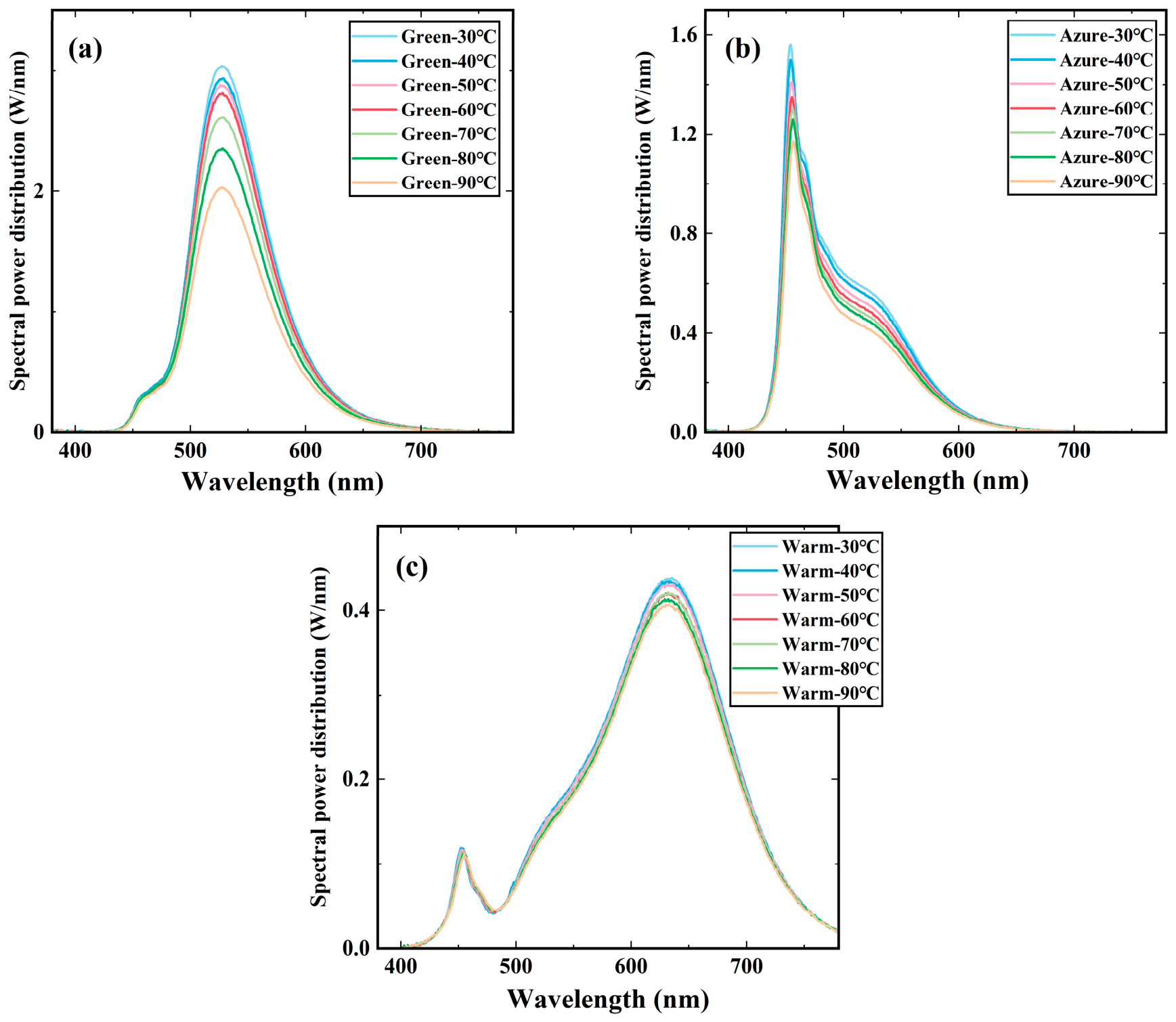
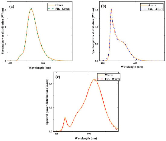
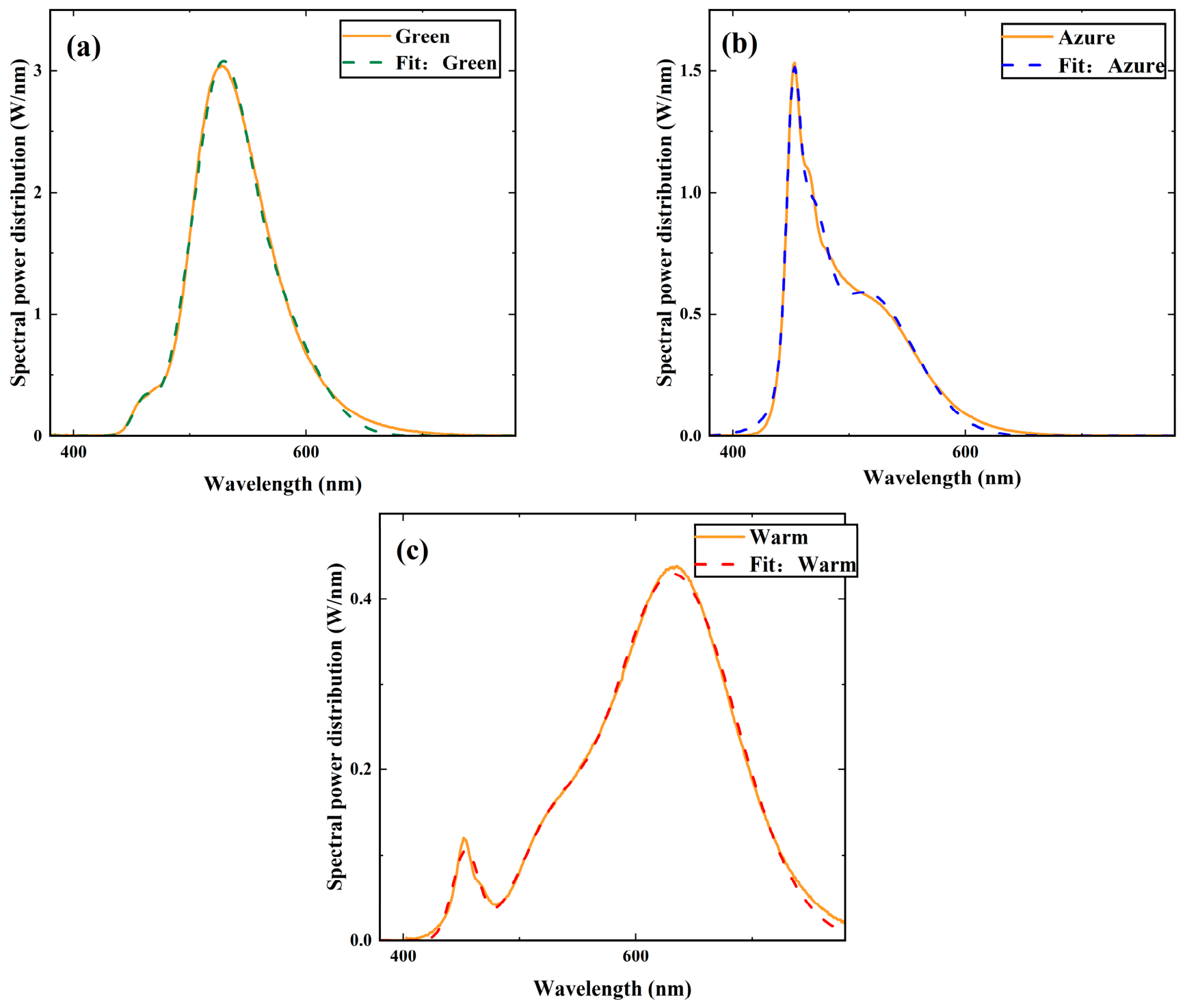
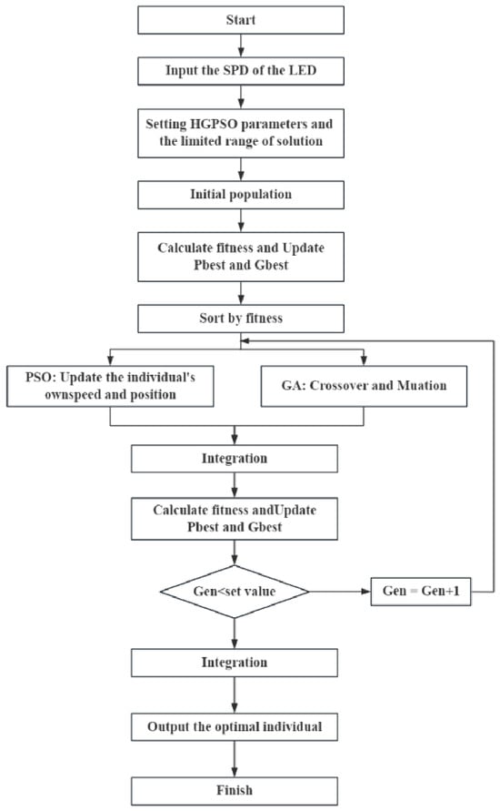
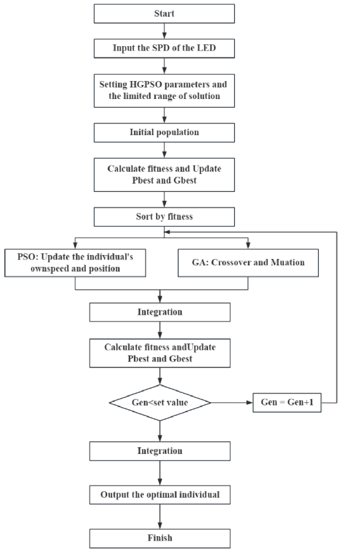
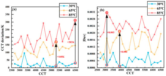
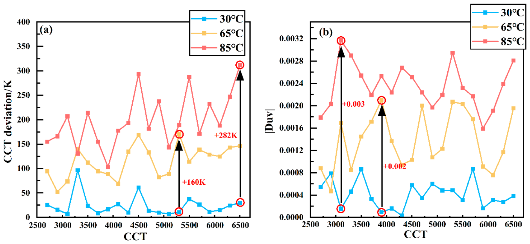
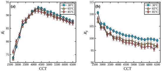
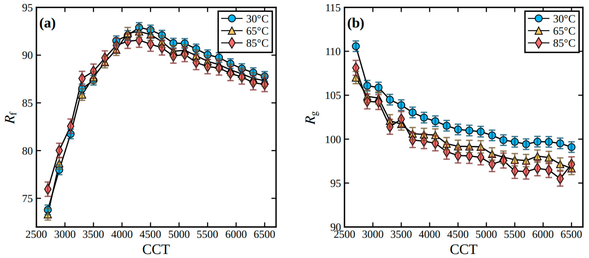
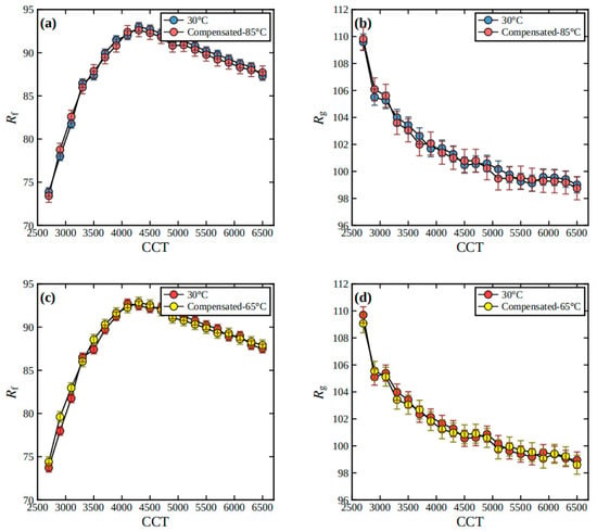
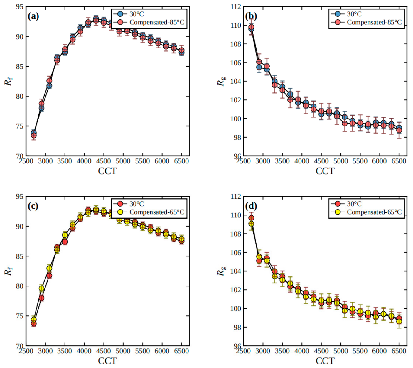
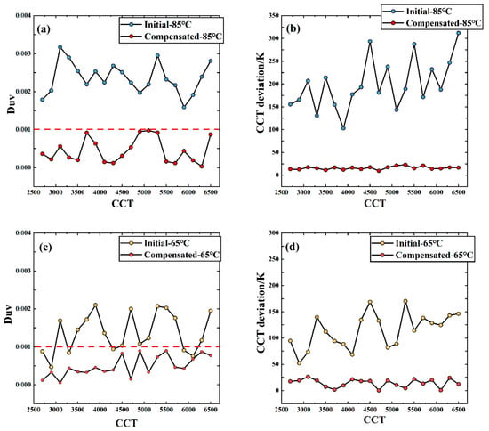
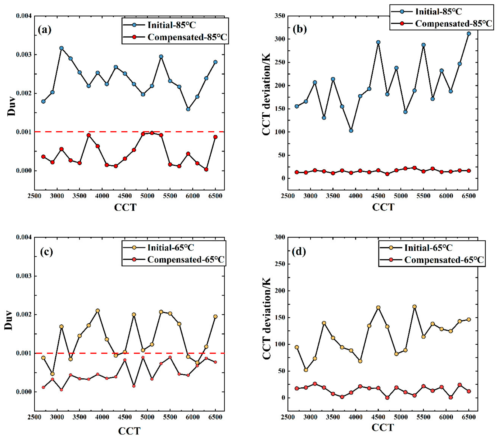
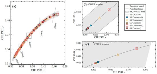
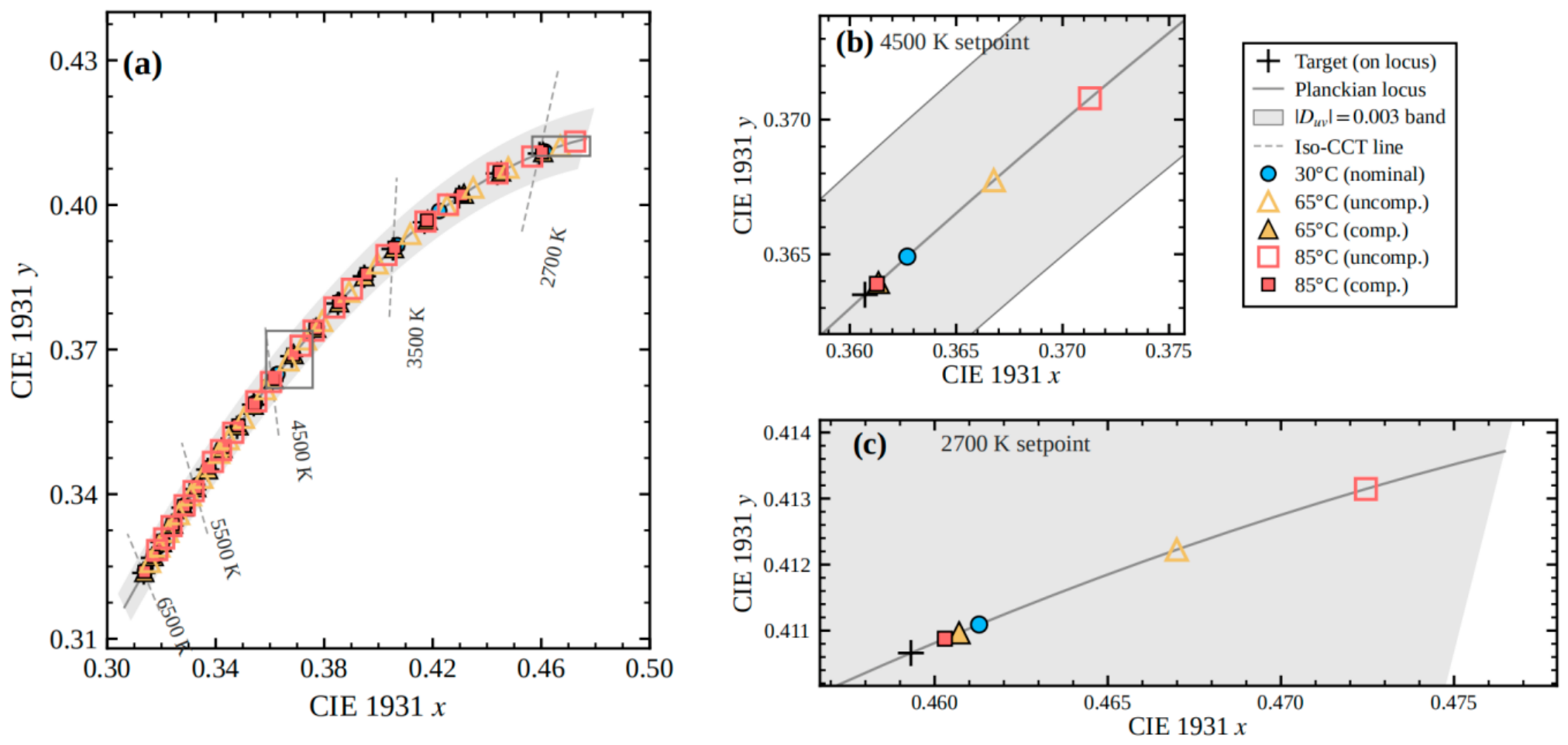
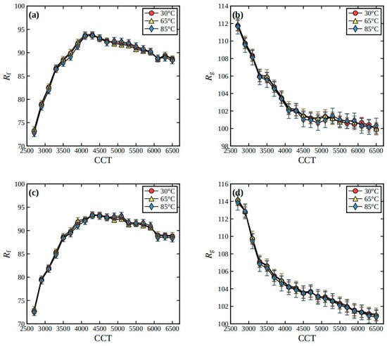
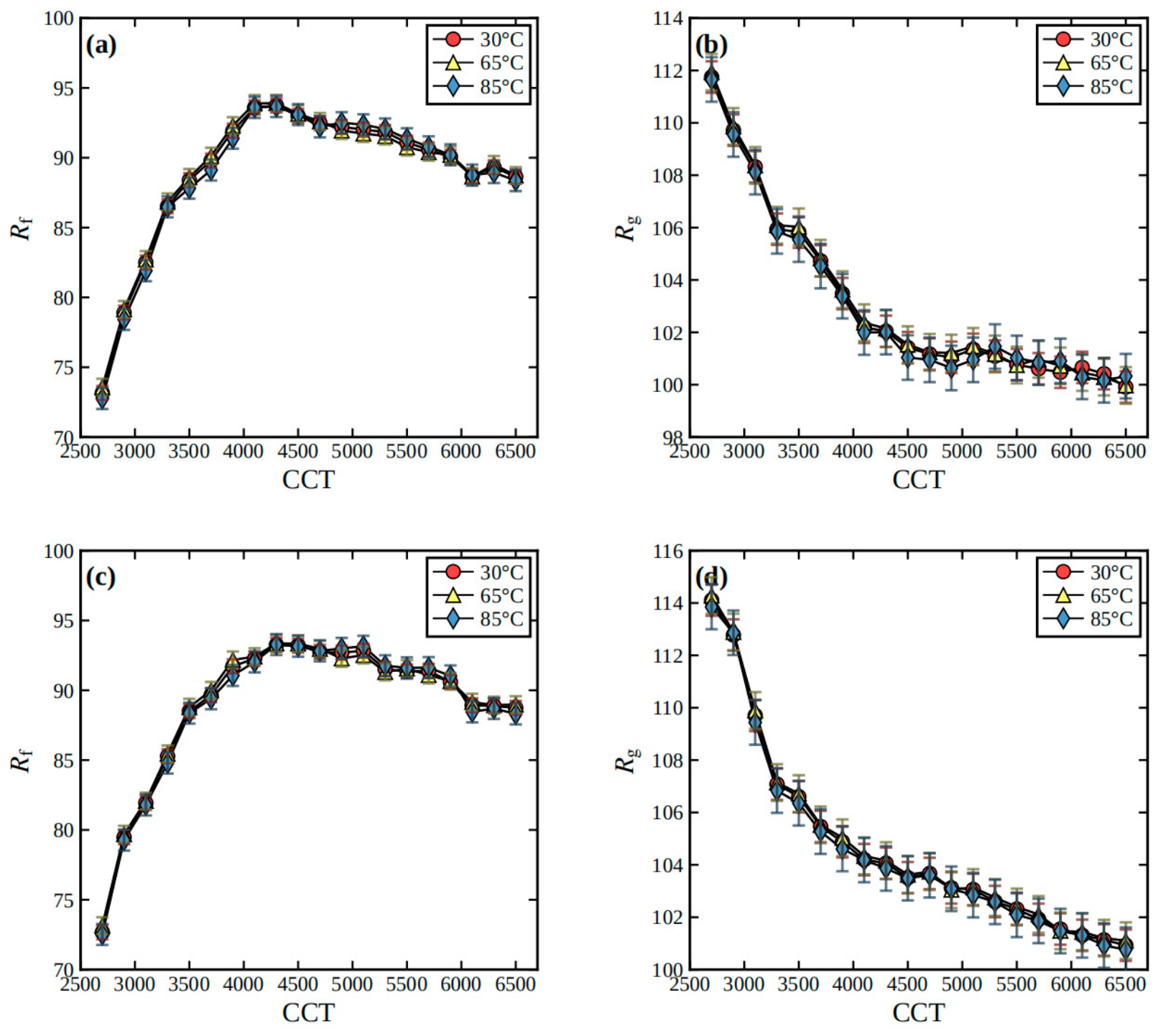
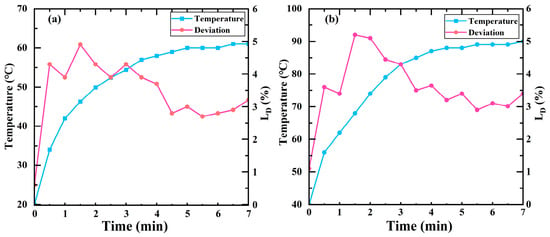
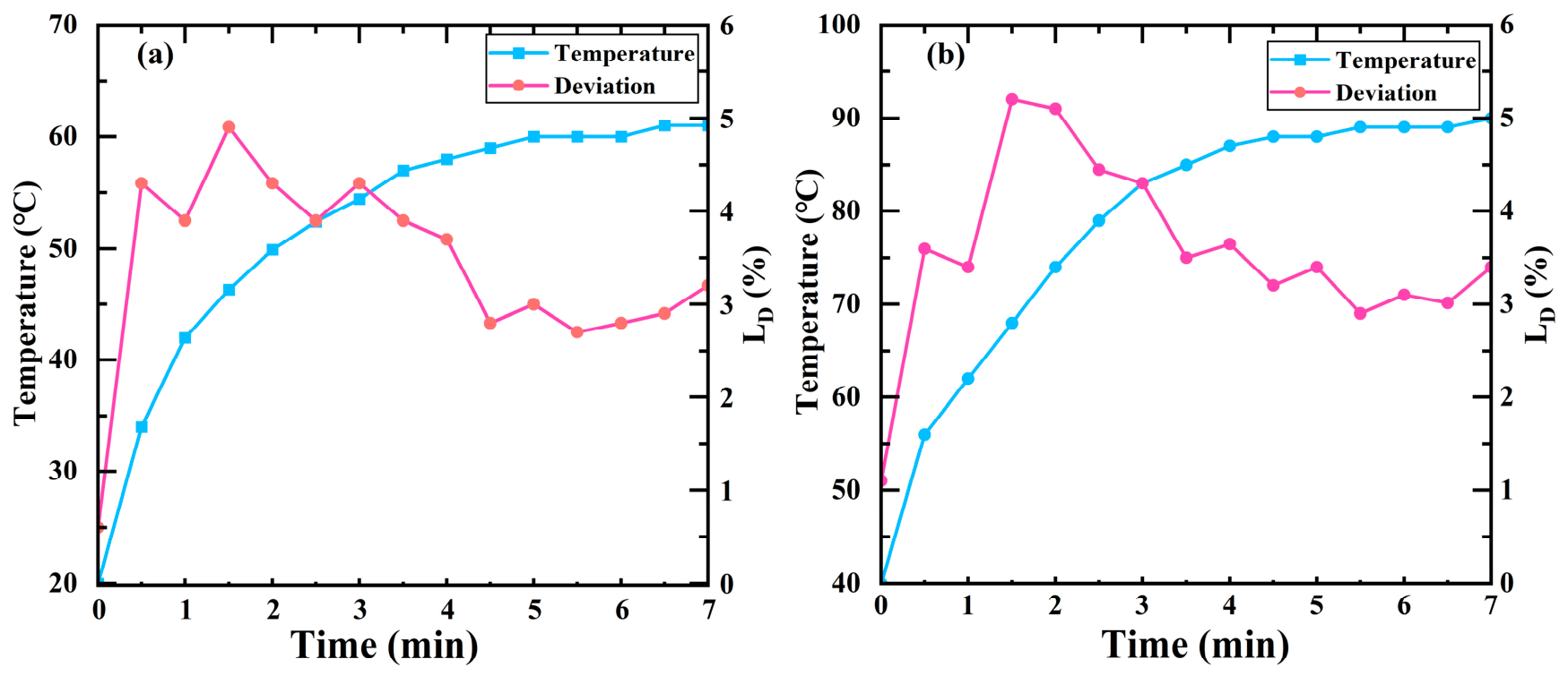
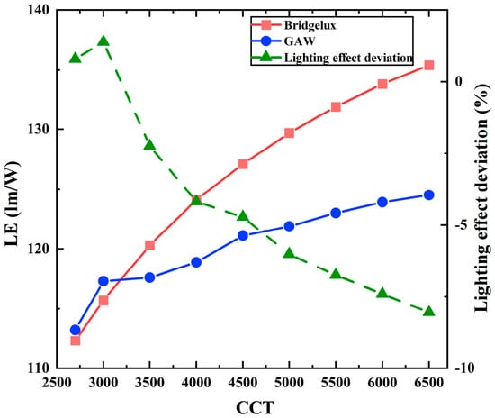
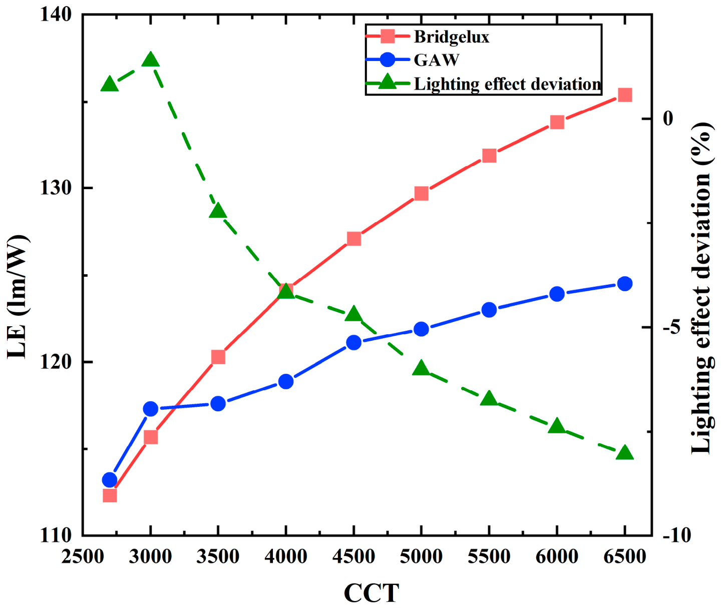
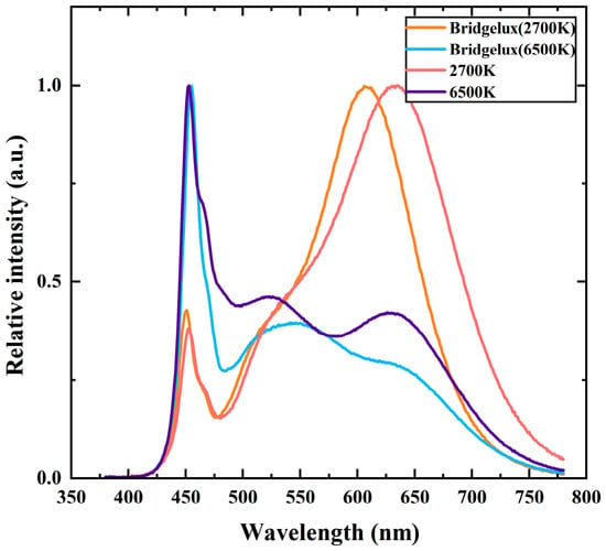
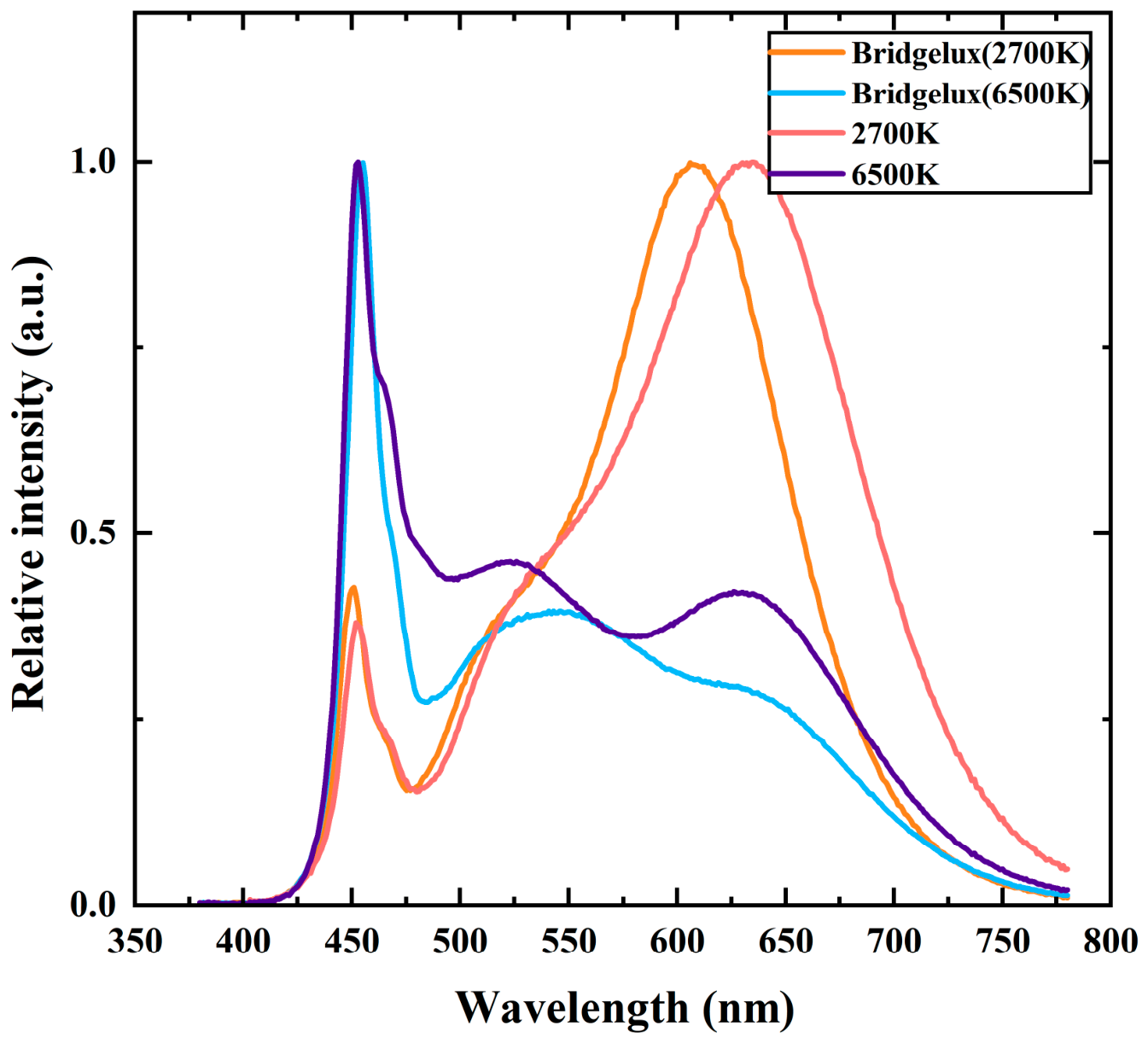
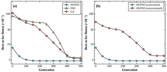
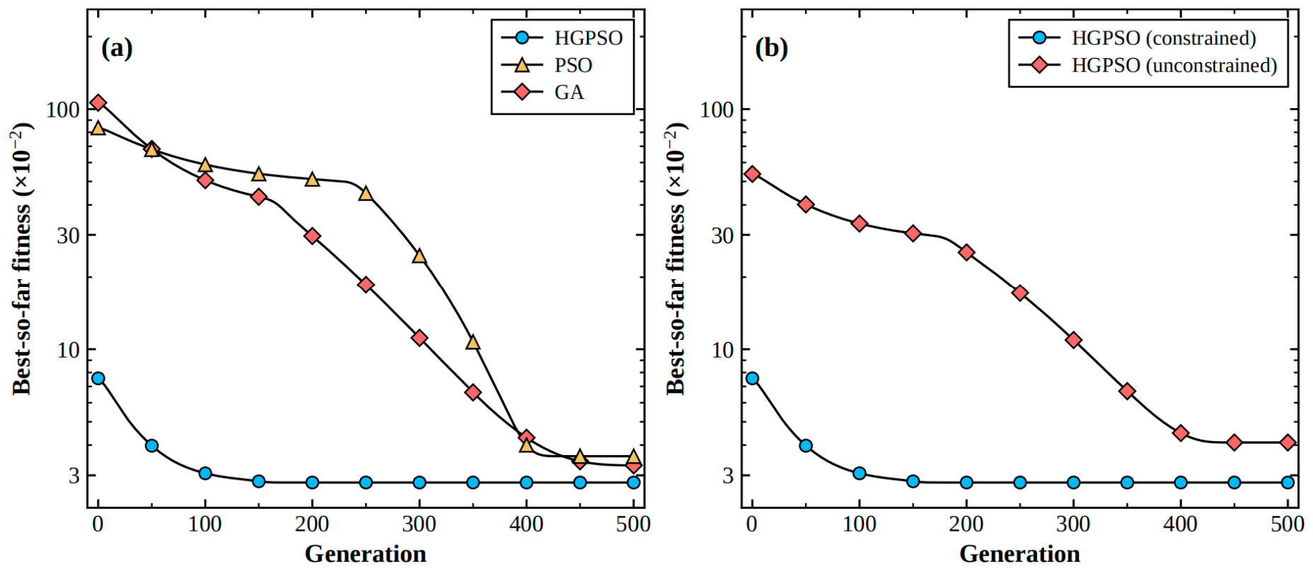

Disclaimer/Publisher’s Note: The statements, opinions and data contained in all publications are solely those of the individual author(s) and contributor(s) and not of MDPI and/or the editor(s). MDPI and/or the editor(s) disclaim responsibility for any injury to people or property resulting from any ideas, methods, instructions or products referred to in the content. |
© 2026 by the authors. Licensee MDPI, Basel, Switzerland. This article is an open access article distributed under the terms and conditions of the Creative Commons Attribution (CC BY) license.