Numerical Analysis of Long-Exposure Imaging Quality in a Joint-Turbulence Environment

Abstract

Refractive index fluctuations in turbulent media severely degrade optical imaging quality. Airborne electro-optic systems often involve optical propagation through both atmospheric turbulence (AT) and compressible turbulence (CT), which forms a joint-turbulence (JT) environment. Current models evaluate this by multiplying the optical transfer functions (OTFs) of individual turbulence types and implicitly assume statistical independence. By analyzing phase fluctuation superposition on the receiving aperture, we derive a new wave-structure function for JT that includes a cross correlation term parameterized by a mutual correlation coefficient. We then establish a long-exposure OTF model for JT imaging which reduces to the conventional method when the fields are uncorrelated. Simulations using resolution test targets and natural scene images evaluated via structural similarity and peak signal-to-noise ratio metrics show that JT degrades image quality significantly more than AT or CT alone. This degradation intensifies monotonically with increases in the correlation coefficient, CT propagation distance, and CT strength. Enlarging the receiving aperture effectively compensates for this degradation. These findings prove that correlation-aware JT models are essential for accurately evaluating image quality and provide a theoretical foundation for advanced-imaging system design.

1. Introduction

When images propagate through turbulent media, random refractive-index fluctuations induce wavefront distortion and intensity scintillation, thereby reducing the resolution and quality of imaging systems [1]. In applications such as airborne electro-optical payloads, laser communications, and remote-sensing imaging, the propagation path often traverses two types of turbulence with distinct physical mechanisms. The first is the extensively studied atmospheric turbulence (AT), whose refractive-index fluctuations arise primarily from temperature fluctuations and obey Kolmogorov statistics in the inertial range [2]. The second is compressible turbulence (CT), which commonly occurs in high-speed aircraft boundary layers, shock boundary-layer interaction regions, and engine wakes [3,4,5]. To model such dynamics, the statistical theory of optical-wave propagation in random media provides a fundamental framework for describing these problems [6]. Recent studies of coherent structures in high-speed boundary layers [7] and aero-optical effects in supersonic turbulent boundary layers [8,9] have further demonstrated that CT differs fundamentally from AT. AT can be regarded as incompressible turbulence, and its refractive-index spectrum follows the Kolmogorov model with a −5/3 power law [10,11]. In contrast, the refractive-index fluctuations in CT arise from temperature and pressure fluctuations. Compressibility modifies the energy spectrum structure and scaling laws and is accompanied by dilatational modes, shock structures, and pronounced anisotropy; consequently, the refractive-index spectrum cannot be described by the classical Kolmogorov model [12,13,14]. In practical imaging links, an optical beam often first passes through a long AT path and then propagates over a CT region near an aircraft before reaching the receiver, together forming a joint-turbulence (JT) environment [15]. Therefore, developing an imaging-degradation model applicable to JT environments is an urgent requirement for the design and image-quality evaluation of electro-optical systems on high-speed platforms.

Research on turbulence-induced imaging degradation has a long history and continues to advance. Fried established the classical theory of long- and short-exposure imaging resolution and introduced the turbulence coherence diameter as a core parameter [16]. Building on this foundation, speckle imaging theory exploits the high-frequency information retained in short-exposure frame sequences to suppress turbulence-induced blur, while the long-exposure modulation- transfer function (MTF) model based on the wave-structure function has become the statistical optics foundation for describing the effect of turbulence on the optical transfer function (OTF) [17]. In recent years, turbulent imaging theory has progressed in several directions. For CT, systematic analyses of aberration sources and imaging-degradation theories have gradually been established [18,19]. Methods for estimating optical turbulence strength in realistic airborne environments have been proposed [20], and selected propagation characteristics of beams in CT have also been investigated [21,22,23]. For transfer function modeling, researchers have developed a wave-structure function and a long-exposure MTF model for Gaussian beams in anisotropic turbulence [24], an average short-exposure MTF theory [25], and an atmospheric MTF model for satellite payloads that accounts for the combined effects of turbulence and aerosols [26]. For numerical simulation, optical simulation based on the phase-screen method has become an important tool for studying turbulent imaging [27]. Wave optics simulations and phase-screen accuracy analyses for non-Kolmogorov turbulence have also been reported [28,29]. Furthermore, research has been conducted on aero-optical effects in compressible flows, as well as wavefront sensing and adaptive optical compensation for airborne platforms [30,31,32]. However, these studies address only a single-turbulence environment, and rely mainly on numerical or experimental methods. Theoretical OTF calculations for JT environments remain immature. Existing practice usually multiplies the OTFs of the two turbulent components directly, which implicitly assumes their statistical independence and neglects the correlation between CT- and AT-induced phase fluctuations. The applicability and accuracy of this treatment have not been systematically evaluated.

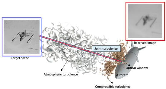
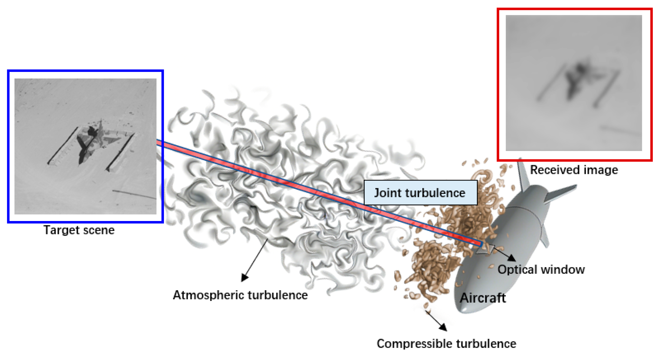
To address these issues, this study starts from the superposition of total phase fluctuations on the receiving aperture, and derives a JT wave-structure function containing a cross term. The cross term is parameterized by a mutual correlation coefficient that characterizes the correlation between AT- and CT- induced phase fluctuations. On this basis, an OTF model for long-exposure imaging in JT environments is established. This model reduces to the conventional OTF product model when the two turbulence fields are statistically independent. The structural similarity index (SSIM) and peak signal-to-noise ratio (PSNR) are then used to quantitatively evaluate image quality. Systematic simulations are performed to analyze the imaging differences among AT, CT, and JT, as well as the effects of the mutual correlation coefficient, CT propagation distance, CT strength, and receiver-aperture diameter on long-exposure JT imaging.The schematic diagram is shown in Figure 1.

Figure 1. Schematic diagram of image transmission in JT.

2. OTF Theory for JT Imaging System

For an incoherent imaging system, the OTF for long-exposure imaging in JT must be derived from the wave-structure function of beam propagation, which characterizes the statistically averaged random phase fluctuations. To derive the OTF for JT, it is necessary to begin with the most fundamental phase fluctuations in the JT field.

2.1. Wave-Structure Function Under JT Coupling

Consider a monochromatic optical wave with wavelength λ propagating through a turbulent medium with refractive-index fluctuations over a distance L, where the wavenumber is k = 2π/λ. The complex amplitude of the optical field at position vector r = (x, y) on the receiving aperture plane can be written as

$$u\left(r\right)=u_0\left(r\right)\exp \left[V_{JT}\left(r\right)+i{\phi }_{JT}\left(r\right)\right]$$

(1)

where $u_0\left(r\right)$ is the complex amplitude of the optical field in free space, $V_{JT}\left(r\right)$ is the log-amplitude fluctuation, which characterizes turbulence-induced intensity fluctuations, and ${\phi }_{JT}\left(r\right)$ is the phase fluctuation, which characterizes turbulence-induced wavefront distortion.

If two types of turbulence with distinct physical mechanisms are present along the propagation path, the total phase fluctuation on the receiving aperture plane can be expressed as

$$\Delta {\phi }_{JT}\left(r\right)=\Delta {\phi }_A\left(r\right)+\Delta {\phi }_C\left(r\right)$$

(2)

where $\Delta {\phi }_A\left(r\right)$ and $\Delta {\phi }_C\left(r\right)$ denote the phase fluctuations induced by AT and CT, respectively.

The wave-structure function is essentially the mean square difference of the complex phase fluctuations between two points r₁ and r₂ on the aperture plane [10]

$$D_{JT}\left(r\right)=⟨{\left|{\phi }_{JT}\left(r_1\right)-{\phi }_{JT}\left(r_2\right)\right|}^2⟩$$

(3)

where $D_{JT}\left(r\right)$ is the wave-structure function of JT, r = |r₁ − r₂| is the magnitude between the two points, and ⟨·⟩ denotes the statistical ensemble average.

Substituting ${\phi }_A\left(r\right)$ and ${\phi }_C\left(r\right)$ into Equation (3) yields

$$\begin{array}{ll}{D}_{JT}\left(r\right)& =⟨{\left|{\phi }_A\left(r_1\right)+{\phi }_C\left(r_1\right)-{\phi }_A\left(r_2\right)-{\phi }_C\left(r_2\right)\right|}^2⟩\\ & =⟨{\left|\left[{\phi }_A\left(r_1\right)-{\phi }_A\left(r_2\right)\right]+\left[{\phi }_C\left(r_1\right)-{\phi }_C\left(r_2\right)\right]\right|}^2⟩\end{array}$$

(4)

The phase difference between positions r₁ and r₂ is ${\phi }_A\left(r_1\right)-{\phi }_A\left(r_2\right)=\Delta {\phi }_A$, ${\phi }_C\left(r_1\right)-{\phi }_C\left(r_2\right)=\Delta {\phi }_C$. Therefore, Equation (4) can be written as

$$\begin{array}{ll}{D}_{JT}\left(r\right)& =⟨{\left|\Delta {\phi }_A+\Delta {\phi }_C\right|}^2⟩\\ & =⟨\Delta {\phi }_A^2⟩+⟨\Delta {\phi }_C^2⟩+2⟨\Delta {\phi }_A\Delta {\phi }_C⟩\end{array}$$

(5)

The first term of the structure function $⟨\Delta {\phi }_A^2⟩$ is precisely the wave-structure function of AT itself $D_A\left(r\right)$. The second term $⟨\Delta {\phi }_C^2⟩$ is the wave-structure function $D_C\left(r\right)$ in CT, and the third term $⟨\Delta {\phi }_A\Delta {\phi }_C⟩$ is the covariance between the differences of the two distinct random fields, denoted here as the cross term $D_{Corss}\left(r\right)$. The cross term characterizes the joint statistical behavior of the phase fluctuations of the two turbulence types at the same pair of spatial points on the receiving plane, and cannot be incorporated into $D_A\left(r\right)$ or $D_C\left(r\right)$. However, there is one relationship that can be confirmed, which is $⟨\Delta {\phi }_A\Delta {\phi }_C⟩\le \sqrt{D_A\left(r\right)D_C\left(r\right)}$. When the two turbulence fields are statistically independent and have zero mean, the cross term vanishes, $⟨\Delta {\phi }_A\Delta {\phi }_C⟩=0$, and Equation (5) reduces to the independent superposition model. When the two fields are considered jointly and their phase fluctuations are positively correlated, the cross term is greater than zero. To parameterize the cross term, we define the cross-correlation coefficient p(r) of the phase fluctuations of the two turbulence types, such that

$$D_{Cross}\left(r\right)=2p\left(r\right)\sqrt{D_A\left(r\right)D_C\left(r\right)}, \left|p\left(r\right)\right|\le 1$$

(6)

where $p\left(r\right)=0$, $p\left(r\right)>0$, and $p\left(r\right)<0$ correspond to statistical independence, positive correlation, and negative correlation, respectively. The upper bound |p(r)| ≤ 1 is guaranteed by the Cauchy–Schwarz inequality. It should be noted that p(r) is a phenomenological parameter, and no established physical model or experimental calibration is currently available for determining its value. Nevertheless, a nonzero correlation between the AT- and CT-induced phase fluctuations is physically plausible. The CT region is not generated in isolation: the boundary layer and wake are produced by the aircraft moving through the atmosphere, and large-scale atmospheric disturbances convect into and modulate the near-airframe flow, so the two turbulent regions are driven by partially common flow states, rather than being strictly unrelated random processes. In addition, aerodynamic heating of the airframe and engine exhaust mix heated air into the downstream atmospheric path, introducing temperature fluctuations that share a common origin with the compressible region, and when the propagation path is short, common large-scale flow structures may span both regions. Accordingly, the value of p is expected to depend on the degree of coupling between the two turbulent regions, including the separation between the AT path and the CT region, the convection time of large-scale structures, and the extent to which density fluctuations in the two regions share such common drivers. For configurations in which a long AT path is followed by a thin near-airframe CT layer, the two regions share only limited common large-scale content, and the correlation is expected to be weak, so that realistic values of p are likely closer to 0 than to 1. A rigorous estimation of p(r) would require synchronized wavefront measurements or coupled flow-field-driven phase-screen simulations, which is left for our future work. In this study, p is therefore treated as a free parameter scanned over its full physical range [0, 1]. p = 0 recovers the conventional independent-superposition model, while p = 1 provides a conservative upper-bound estimate of the cross-term contribution, rather than a typical value. For simplicity, p is assumed constant over the receiving aperture in the simulations.

This constant p assumption can be interpreted as an effective, aperture-averaged value of p(r) over the range of separations r $\in$ (0, D₀) that contribute to the long-exposure OTF. The actual r-dependence of p is currently unknown, and cannot be determined without experimental data; moreover, it need not follow the decaying trend typical of other second-order statistics, since the phase increments at small separations are dominated by the largely independent small-scale fluctuations of the two regions, whereas the shared large-scale flow structures contribute increasingly at larger separations. Because any assumed functional form of p(r) would introduce additional unknown parameters without experimental support, a constant p is the only parameter-free closure.

Therefore, the total wave-structure function is

$$D_{JT}\left(r\right)=D_A\left(r\right)+D_C\left(r\right)+2p\left(r\right)\sqrt{D_A\left(r\right)D_C\left(r\right)}$$

(7)

To determine the wave-structure function in JT, it is necessary to derive the wave-structure functions for AT and CT separately. For AT, the wave-structure function has been derived theoretically. Here, we directly adopt the plane wave-structure function based on the Kolmogorov spectrum [17]

$$D_A\left(r\right)=2.91k^2{L}_{AT}{C}_n^2{r}^{5/3}$$

(8)

where $L_{AT}$ is the propagation distance through AT and is the atmospheric refractive-index structure constant.

In CT, $D_C\left(r\right)$ can be expressed in the general form of the plane wave-structure function [17]

$$D_C\left(r\right)=8{\pi }^2{k}^2{L}_{CT}{\displaystyle {\int }_0^{\infty }\kappa {\Phi }_{n,\mathrm{CT}}\left(\kappa \right)\left[1-J_0\left(\kappa r\right)\right]\mathrm{d}\kappa }$$

(9)

where $J_0$ is the zero-order Bessel function of the first kind. The refractive-index fluctuations for beam propagation in CT are modeled using the temperature and pressure co-spectrum ${\Phi }_{n,\mathrm{CT}}\left(\kappa \right)$, given by [5]:

$$\begin{array}{ll}{\Phi }_{n,\mathrm{CT}}\left(\kappa \right)={\displaystyle \frac{{\left(K_{GD}{\overline{\rho }}^2\gamma R\overline{T}\right)}^2}{4\pi {\overline{a}}^2{\overline{P}}^2}}& \left[B_P{\epsilon }^{4/3}{y}^{-4/3}{l}_{\mathrm{CT}}^{13/3}{\left(1+{\kappa }^2{l}_{\mathrm{CT}}^2\right)}^{-13/6}\right.\\ & \left.+R^2\beta \chi {\epsilon }^{-1/3}{l}_{\mathrm{CT}}^{11/3}{\left(1+{\kappa }^2{l}_{\mathrm{CT}}^2\right)}^{-11/6}\right]\end{array}$$

(10)

where $\gamma$ is the ratio of specific heats for air, and $K_{GD}$ is the G-D constant, which is a parameter related to the optical wavelength. $\overline{\rho }$, $\overline{T}$, and $\overline{P}$ are the average air density, temperature, and pressure, respectively. y is the distance of the turbulence from the wall, $\overline{a}$ is the average value of sound velocity, $B_P$ is a dimensionless constant, $\epsilon$ is the turbulence-dissipation rate, and l_CT is the characteristic length scale (l_CT = L_0,CT/2π, and L_0,CT is the outer scale of turbulence). R is the gas constant, $\beta$ is a nondimensional constant, and $\chi$ is the average temperature-dissipation rate. The spectrum in Equation (10) was derived in Ref. [5] from the velocity structure function of compressible flow with nonzero divergence, combined with the Gladstone–Dale relation and a simplified van der Waals equation of state. In this model, the refractive-index fluctuations are jointly determined by the pressure spectrum and the temperature spectrum, resulting in a three-dimensional spectral slope between −11/3 and −13/3, rather than the single −11/3 slope of the Kolmogorov model. The theoretical spectrum has been validated against NPLS wind-tunnel experiments at Ma = 3 and Re = 7.65 × 10⁵, in which the measured slopes of the wavefront amplitude spectrum (−5/3 to −7/3) and the deflection-angle amplitude spectrum (−2/3 to −4/3) agree well with the theoretical predictions in the inertial subrange. The spectrum in Equation (10) assumes a zero inner-scale model for CT. This assumption is justified for the present imaging analysis because the long-exposure OTF is dominated by inertial-range phase statistics at aperture-scale separations (r ≤ D₀), to which dissipation-range scales contribute negligibly. A finite inner-scale model would mainly refine the high-wavenumber asymptotic behavior, and is left for future work.

For computational convenience, we denote the constant term in Equation (10):

$$C_1={\displaystyle \frac{{\left(K_{GD}{\overline{\rho }}^2\gamma R\overline{T}\right)}^2}{4\pi {\overline{a}}^4{\overline{P}}^2}}{B}_P{\epsilon }^{4/3}{y}^{-4/3},C_2={\displaystyle \frac{{\left(K_{GD}{\overline{\rho }}^2\gamma R\overline{T}\right)}^2}{4\pi {\overline{a}}^4{\overline{P}}^2}}{R}^2\beta \chi {\epsilon }^{-1/3}$$

(11)

When Equations (10) and (11) are substituted into Equation (9), the second-order approximation of the Bessel function cannot be used. Otherwise, the integral diverges because the refractive-index spectrum has not yet been corrected for the turbulence scales. Direct integration must therefore be used, yielding

$$\begin{array}{c}{D}_C\left(r\right)=8{\pi }^2{k}^2{L}_{CT}\left\{{\displaystyle \frac{3}{7}}{l}_{CT}^{7/3}{C}_1+{\displaystyle \frac{3}{5}}{l}_{CT}^{5/3}{C}_2\right.-\left[C_1{\displaystyle \frac{l_{CT}^{7/6}}{2^{7/6}\Gamma \left(13/6\right)}}{r}^{7/6}{K}_{-7/6}\left(\frac{r}{l_{CT}}\right)\right.\\ \left.\left.+C_2{\displaystyle \frac{l_{CT}^{5/6}}{2^{5/6}\Gamma \left(11/6\right)}}{r}^{5/6}{K}_{-5/6}\left(\frac{r}{l_{CT}}\right)\right]\right\}\end{array}$$

(12)

where $K_{-7/6}(r/l_{CT})$ and $K_{-5/6}(r/l_{CT})$ are the modified Bessel functions of the second kind of orders −6/7 and −5/6, respectively. For computational convenience, the modified Bessel functions of the second kind can be expanded as a series:

$$\begin{array}{l}{K}_{7/6}\left(\frac{r}{l_{CT}}\right)={\displaystyle \frac{2^{1/6}\Gamma \left(7/6\right)}{{\left(\frac{r}{l_{CT}}\right)}^{7/6}}}-{\displaystyle \frac{3\Gamma \left(7/6\right)}{2^{5/6}}}{\left(\frac{r}{l_{CT}}\right)}^{5/6}+{\displaystyle \frac{\Gamma \left(-7/6\right)}{2^{13/6}}}{\left(\frac{r}{l_{CT}}\right)}^{7/6}+o{\left[\frac{r}{l_{CT}}\right]}^{17/6}\\ K_{5/6}\left(\frac{r}{l_{CT}}\right)={\displaystyle \frac{\Gamma \left(5/6\right)}{2^{1/6}{\left(\frac{r}{l_{CT}}\right)}^{5/6}}}+{\displaystyle \frac{\Gamma \left(-5/6\right)}{2^{11/6}}}{\left(\frac{r}{l_{CT}}\right)}^{5/6}+{\displaystyle \frac{3\Gamma \left(5/6\right)}{2^{7/6}}}{\left(\frac{r}{l_{CT}}\right)}^{7/6}+o{\left[\frac{r}{l_{CT}}\right]}^{17/6}\end{array}$$

(13)

where $o{\left[r/l_{CT}\right]}^n$ denotes higher-order infinitesimal terms. Since $r/l_{CT}\ll 1$, substituting Equation (13) into Equation (12) yields the approximate plane wave-structure function

$$\begin{array}{c}{D}_C(r)\approx 8{\pi }^2{k}^2{L}_{CT}\left\{C_1\left[{\displaystyle \frac{3l_{CT}^{1/3}\Gamma \left(7/6\right)}{4\Gamma \left(13/6\right)}}{r}^2-{\displaystyle \frac{\Gamma \left(-7/6\right)}{2^{10/3}\Gamma \left(13/6\right)}}{r}^{7/3}\right]\right.\\ \left.-C_2\left[{\displaystyle \frac{\Gamma \left(-5/6\right)}{2^{8/3}\Gamma \left(11/6\right)}}{r}^{5/3}+{\displaystyle \frac{3\Gamma \left(5/6\right)}{4l^{1/3}\Gamma \left(11/6\right)}}{r}^2\right]\right\}\end{array}$$

(14)

Finally, substituting Equations (8), (14), and (7) yields the wave-structure function in JT.

2.2. Long-Exposure OTF

For an incoherent imaging system, the long-exposure OTF is the statistical average of the autocorrelation of the pupil function over the random wavefront, and its turbulence-induced component satisfies [17]:

$$OT{F}_{JT}=\exp \left[-{\displaystyle \frac{1}{2}}{D}_{JT}\left(r\right)\right], r=\lambda L_{Total}\left|f\right|$$

(15)

where f = (f_x, f_y) is the spatial frequency, with units of m⁻¹, and r = λL|f| gives the correspondence between spatial frequency and r. Under long-exposure conditions, the ensemble average of the phase transfer function (PTF) is zero for the zero-mean turbulent phase. Consequently, $OT{F}_{JT}$ reduces to a real quantity and is equivalent to the modulation transfer function (MTF).

Therefore, $OT{F}_{JT}$ can be expressed as

$$OT{F}_{JT}=\exp \left\{-{\displaystyle \frac{1}{2}}\left[D_A\left(\lambda L_{AT}f\right)+D_C\left(\lambda L_{CT}f\right)+2p\left(\lambda L_{Total}f\right)\sqrt{D_A\left(\lambda L_{AT}f\right)D_C\left(\lambda L_{CT}f\right)}\right]\right\}$$

(16)

where $L_{Total}$ is the total propagation distance.

The OTF of the entire system can then be expressed as

$$OT{F}_{Total}=OT{F}_{static}\cdot OT{F}_{JT}$$

(17)

where $OT{F}_{static}$ is the ideal static statistical OTF. For a circular-aperture diffraction-limited system, the ideal static statistical OTF can be written as [17]:

$$H_{\mathrm{static}}\left(\frac{f}{f_c}\right)={\displaystyle \frac{2}{\pi }}\left[{\cos }^{-1}\left(\frac{f}{f_c}\right)-{\displaystyle \frac{f}{f_c}}\sqrt{1-{\left(\frac{f}{f_c}\right)}^2}\right]$$

(18)

where $f_c=D_0/\left(\lambda L_{\mathrm{total}}\right)$ is the cutoff frequency, and D₀ is the receiver-aperture diameter. For an image $I_{in}\left(x,y\right)$, the transmitted image can be expressed as

$$I_{\mathrm{out}}\left(x,y\right)={\mathcal{F}}^{-1}\left[G_{in}\left(f_x,f_y\right)\cdot OT{F}_{Total}\left(f_x,f_y\right)\right], G_{in}\left(f_x,f_y\right)=\mathcal{F}\left[I_{in}\left(x,y\right)\right]$$

(19)

where $G_{in}\left(f_x,f_y\right)$ is the spectrum of the input image, $\mathcal{F}$ denotes the Fourier transform, ${\mathcal{F}}^{-1}$ denotes the inverse Fourier transform, $f_x$ and $f_y$ are the x and y components of the spatial frequency f, respectively, and $f=\sqrt{f_x^2+f_y^2}$.

3. Results

Unless otherwise specified, the parameters for analyzing beam-propagation characteristics are selected as follows: AT parameters $C_n^2={10}^{-16}{\mathrm{m}}^{-2/3}$, L_AT = 2000 m, and CT parameters $B_p=8$, $\epsilon =0.5 {\mathrm{m}}^{-2}\cdot {\mathrm{s}}^{-3}$, $R=8.31 \mathrm{J}\cdot {\left(\mathrm{mol}\cdot \mathrm{K}\right)}^{-1}$, $\beta =0.8$, $\chi \approx 1 {\mathrm{K}}^2\cdot {\mathrm{s}}^{-1}$ [33,34], $y\approx L_{\mathrm{CT}}$. Therefore, $C_1/C_2\approx 0.0365$, and taking $C_2={10}^{-9}{\mathrm{m}}^{-2/3}$, l_CT = 0.4 m, L_CT = 1.0 m, the transmission distance is determined by the shock-wave/boundary-layer interaction region thickness, and is typically within a few tens of centimeters. Since oblique incidence increases the transmission distance, a value of less than 1.0 m is adopted here. Here, C₂ is defined as the constant prefactor of the CT refractive-index spectrum in Equation (10), which characterizes the intensity of refractive-index fluctuations in CT, analogous to the role of $C_n^2$ in AT. It should be noted that C₂ is not a purely empirical parameter: through the spectrum model of Equation (10), it is indirectly related to the characteristic flow parameters of the compressible flow, such as the Mach number and the Reynolds number, since these parameters determine the mean flow state and the turbulence-dissipation rates that enter the spectrum. C₂ typically takes a value between 10⁻¹⁰ and 10⁻⁷ m^−2/3. The sampling frequency is df = 1/w₀, where w₀ = 0.3 m is the target scene width, the receiver aperture is D₀ = 0.3 m, and the mutual correlation coefficient of the JT is p = 1; the value p = 1 is adopted as a conservative worst-case choice. It should be emphasized that p = 1 is an idealized upper-bound case, rather than a generic JT condition. Because the cross term enters D_JT with a positive sign, p = 1 maximizes the wave-structure function and therefore corresponds to the worst-case degradation of the imaging quality, while p = 0 gives the lower bound. A near-unity p could arise physically when both segments are driven by common large-scale structures, e.g., when the atmospheric path traverses the extended turbulent wake of the aircraft, rather than quiescent free atmosphere.

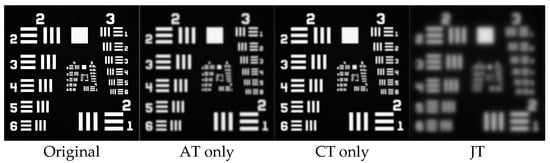
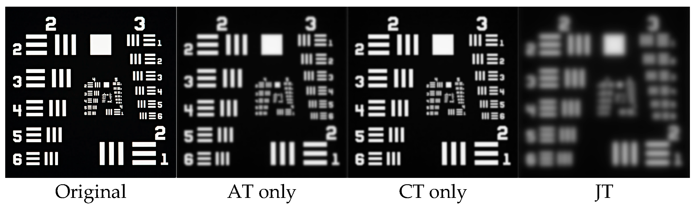
Figure 2 and Table 1 present the long-exposure imaging results obtained after the Resolution Test Target (RTT) image propagates through AT, CT, and JT, respectively. All three turbulence environments cause varying degrees of edge blur in the bars and reduced contrast of the group numbers. Notably, the PSNR under JT is approximately 4.50 dB and 6.83 dB lower than those under AT and CT, while the SSIM under JT is approximately 0.14 and 0.22 lower. These results indicate that the degradation under JT arises from the coupling of the two turbulence components. As shown in Figure 2, some bars are difficult to distinguish in the JT image, whereas the corresponding bars remain identifiable in the AT and CT images. This demonstrates that the high-frequency components abundant in the resolution target are highly sensitive to the high-frequency attenuation of the turbulence MTF and can directly reveal the additional loss of imaging resolution caused by JT coupling.

Figure 2. Long-exposure RTT images in different turbulence environments (from left to right: original, AT only, CT only, JT with p = 1); L_AT = 2000 m, L_CT = 1.0 m, C₂ = 10⁻⁹ m^−2/3, D₀ = 0.3 m. The corresponding SSIM and PSNR values are listed in Table 1.

Table 1. SSIM and PSNR of each long-exposure image in Figure 2 compared with the original image.

	AT Only	CT Only	JT
SSIM	0.6856	0.7608	0.5412
PSNR (dB)	15.1151	17.4478	10.6169

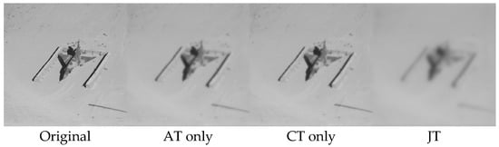
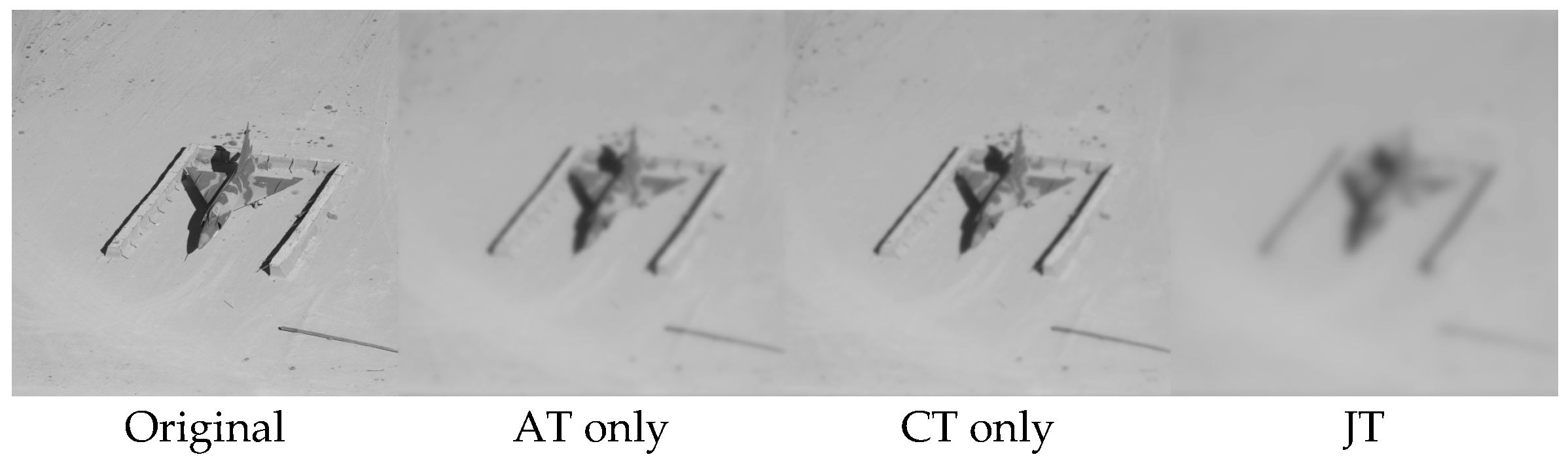
Figure 3 and Table 2 show the results for the Airplane image. Compared with Figure 2, the image-quality metrics under all three turbulence conditions are markedly higher. The difference between the two sets of images primarily results from their different target spectrum distributions. The energy of the natural image is concentrated in the low-frequency region, whereas the long-exposure turbulence in the MTF model decreases monotonically with spatial frequency. Low-frequency components are therefore less affected by turbulence, making the Airplane image less sensitive to turbulence than the RTT. This comparison demonstrates that the severity of turbulence-induced imaging degradation must be evaluated in conjunction with the spectral characteristics of the target. The richer the high-frequency details of the target, the more significant the additional image-quality loss caused by the coupling of the two turbulence components.

Figure 3. Long-exposure Airplane images in different turbulence environments (from left to right: original, AT only, CT only, JT with p = 1); parameters are the same as in Figure 2, with metrics in Table 2.

Table 2. SSIM and PSNR of each long-exposure image in Figure 3 compared with the original image.

	AT Only	CT Only	JT
SSIM	0.8574	0.8823	0.8305
PSNR (dB)	27.0395	29.1459	23.3639

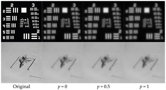
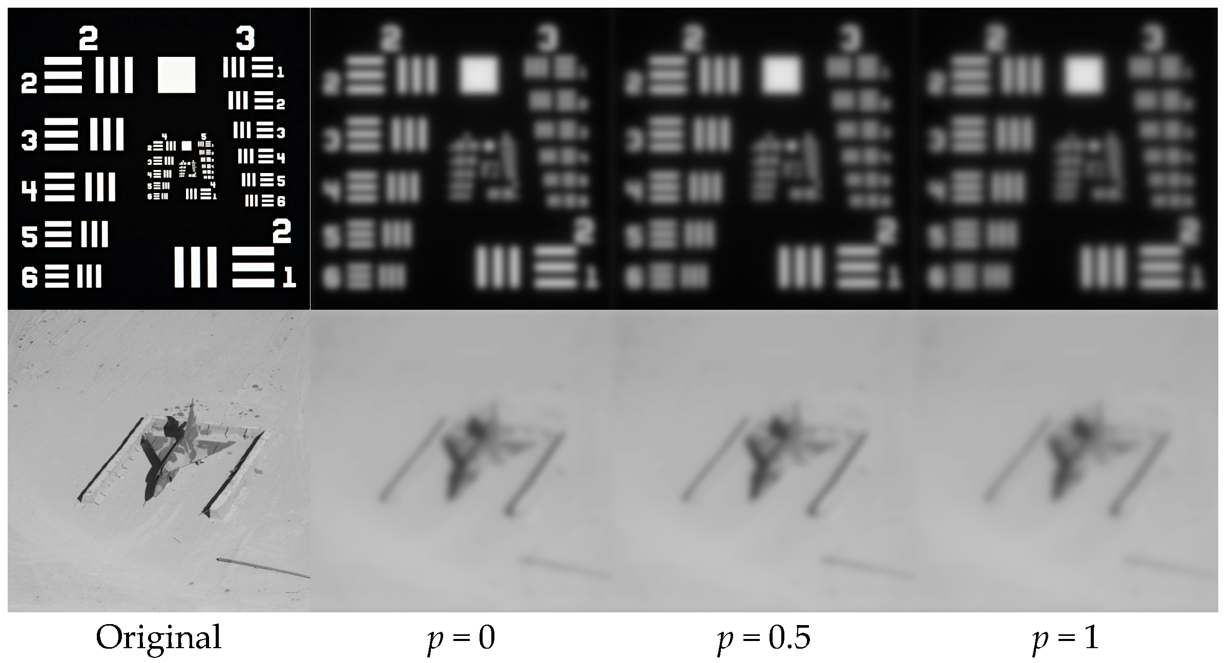
Figure 4 and Table 3 examine the effect of the mutual correlation coefficient p in JT on long-exposure imaging. As p increases from 0 to 1, the SSIM and PSNR of both target images decrease monotonically. The PSNR of the RTT decreases from 11.24 dB to 10.62 dB, while that of the Airplane image decreases from 23.89 dB to 23.36 dB. The case p = 0 corresponds to statistical independence between the two turbulence components, under which the joint wave-structure function reduces to the simple sum of the individual AT and CT wave-structure functions, which is the conventional OTF product model. An increase in p indicates stronger correlation between the phase fluctuations of the two turbulence components. The resulting cross term increases the total wave-structure function. These results show that the independent superposition assumption systematically overestimates image quality in JT environments. For the RTT, this overestimation reaches approximately 0.6 dB at p = 1. The cross-term correction is the key distinction between the proposed JT imaging theory and the conventional superposition model, and is necessary for explaining the additional resolution loss in coupled turbulence.

Figure 4. Long-exposure RTT and Airplane images in JT with different mutual correlation coefficients (from left to right: original, p = 0, 0.5, 1); other parameters are the same as in Figure 2, with metrics in Table 3.

Table 3. SSIM and PSNR of each long-exposure image in Figure 4 compared with the original image.

	p = 0	p = 0.5	p = 1
SSIM (RTT)	0.5639	0.5517	0.5412
PSNR (RTT) (dB)	11.2361	10.8958	10.6169
SSIM (Airplane)	0.8329	0.8315	0.8305
PSNR (Airplane) (dB)	23.8908	23.6000	23.3639

From a practical perspective, the sensitivity of the predicted image quality to the uncertainty in p is weak: the dependence is approximately linear, and an uncertainty of Δp = 0.1 corresponds to only about 0.06 dB (RTT) and 0.05 dB (Airplane) in PSNR. The total variation over the full range p $\in$ [0, 1] (about 0.6 dB for the RTT) is also much smaller than the degradation gap between JT and a single turbulence component (4.5–6.8 dB).

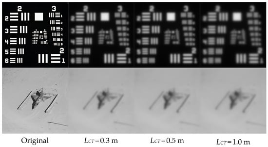
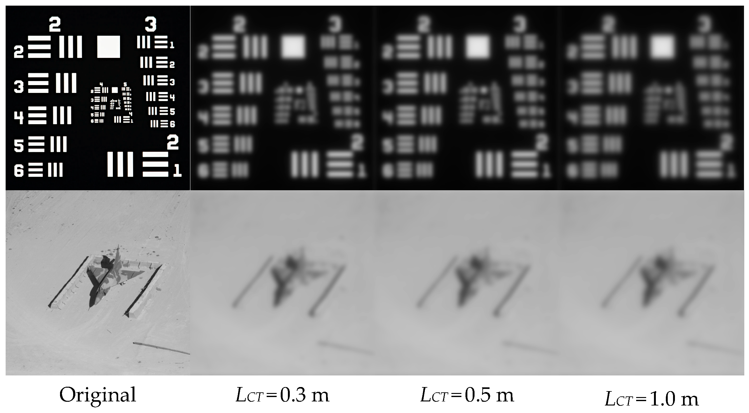
Figure 5 and Table 4 show the variation in long-exposure images as the CT propagation distance L_CT increases from 0.3 m to 1.0 m. With increasing L_CT, the image quality of both targets decreases monotonically. The PSNR of RTT decreases from 11.34 dB to 10.62 dB, while that of the Airplane image decreases from 23.98 dB to 23.36 dB. This trend arises from the cumulative effect of the CT wave-structure function with propagation distance; a larger L_CT increases the contribution of CT to the total wave-structure function, reduces the equivalent coherence diameter, and produces stronger MTF attenuation. It should be emphasized that, although the CT interaction distance (on the order of meters) is much shorter than the AT propagation distance (2000 m), the resulting image-quality degradation is comparable to that caused by AT. This indicates that the wavefront disturbance per unit length in CT is much stronger than that in conventional AT. Therefore, in imaging links containing compressible regions such as boundary layers or high-speed flows, even a thin compressible region must be incorporated into the JT model; otherwise, the actual degradation will be significantly underestimated.

Figure 5. Long-exposure RTT and Airplane images in JT at different CT propagation distances (from left to right: original, L_CT = 0.3, 0.5, 1.0 m; p = 1); other parameters are the same as in Figure 2, with metrics in Table 4.

Table 4. SSIM and PSNR of each long-exposure image in Figure 5 compared with the original image.

	LCT = 0.3 m	LCT = 0.5 m	LCT = 1.0 m
SSIM (RTT)	0.5674	0.5611	0.5412
PSNR (RTT) (dB)	11.3387	11.1578	10.6169
SSIM (Airplane)	0.8333	0.8326	0.8305
PSNR (Airplane) (dB)	23.9786	23.8237	23.3639

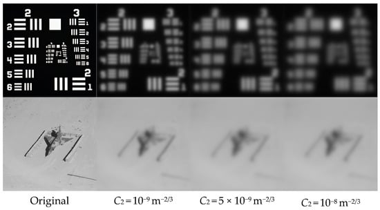
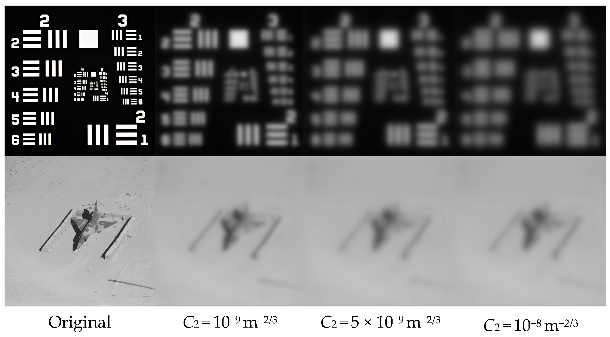
Figure 6 and Table 5 examine the effect of CT strength (represented by C₂, similar to the structure constant $C_n^2$, characterizing the intensity of turbulent fluctuations), which increases from 10⁻⁹ m^−2/3 to 10⁻⁸ m^−2/3. As C₂ increases, the image quality deteriorates markedly. The PSNR of the RTT decreases successively, from 10.62 dB to 9.61 dB and 8.83 dB, while the SSIM decreases from 0.5412 to 0.4764. The PSNR of the Airplane image decreases from 23.36 dB to 22.17 dB. This behavior occurs because C₂ is physically analogous to $C_n^2$ in AT, and characterizes the magnitude of refractive-index fluctuations in CT. When C₂ increases by approximately one order of magnitude, the PSNR of the bar target decreases by approximately 1.79 dB. A comparison with Table 1 shows that, at C₂ = 10⁻⁸ m^−2/3, the difference between the JT image (8.83 dB) and AT alone (15.12 dB) exceeds 6 dB, indicating that CT can then dominate the JT environment and become the primary factor limiting imaging quality.

Figure 6. Long-exposure RTT and Airplane images in JT under different CT strengths (from left to right: original, C₂ = 10⁻⁹, 5 × 10⁻⁹, 10⁻⁸ m^−2/3; p = 1, L_CT = 1.0 m); metrics in Table 5.

Table 5. SSIM and PSNR of each long -xposure image in Figure 6 compared with the original image.

	C2 = 10−9 m−2/3	C2 = 5 × 10−9 m−2/3	C2 = 10−8 m−2/3
SSIM (RTT)	0.5412	0.5022	0.4764
PSNR (RTT) (dB)	10.6169	9.6134	8.8276
SSIM (Airplane)	0.8305	0.8279	0.8270
PSNR (Airplane) (dB)	23.3639	22.5957	22.1651

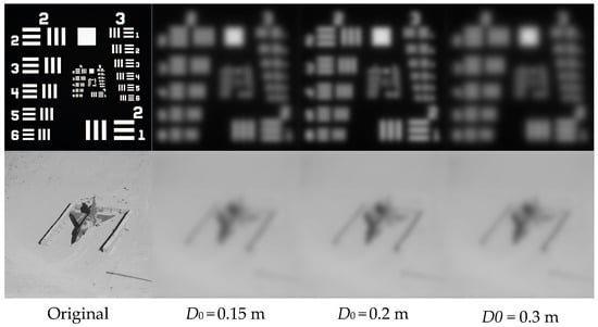
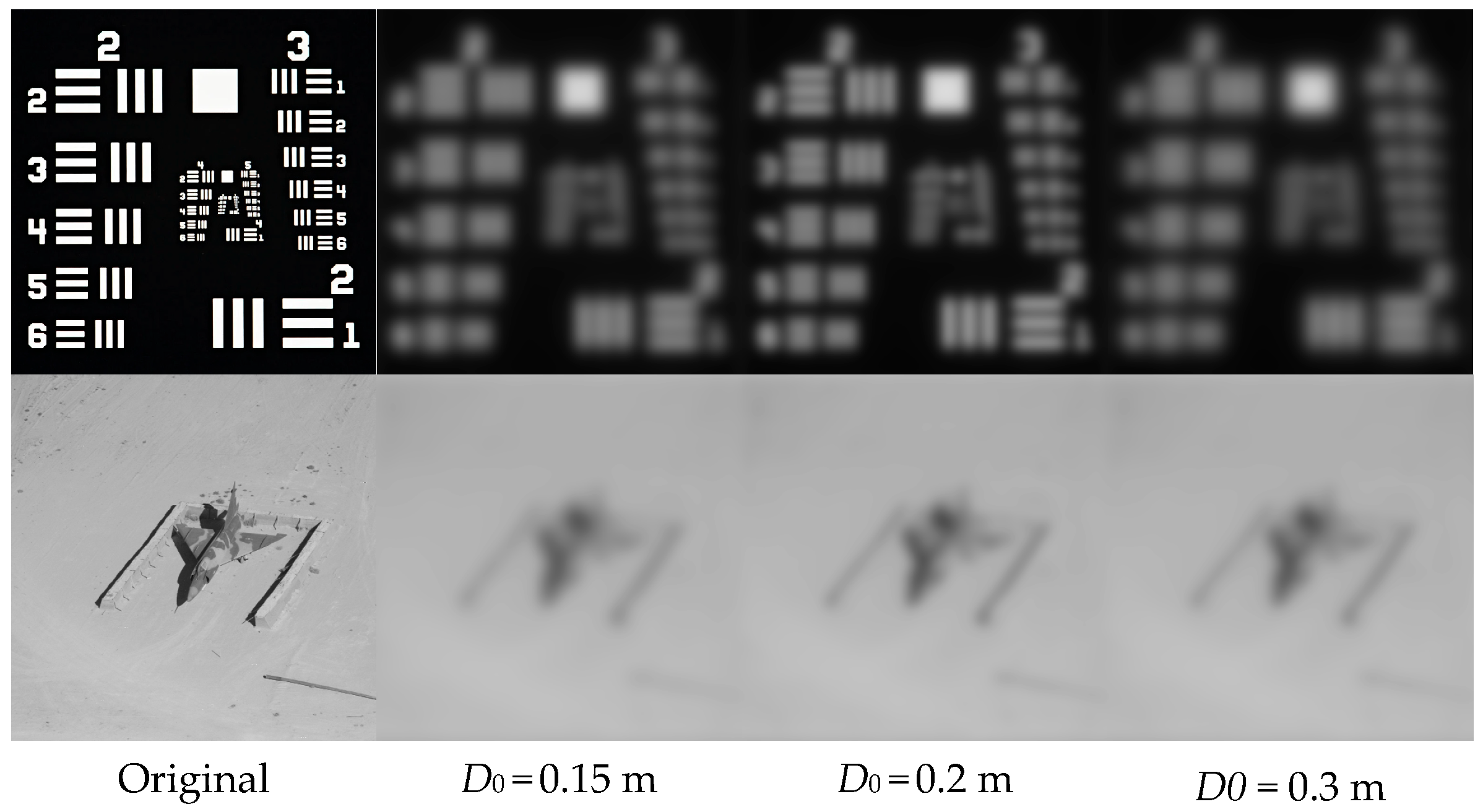
Figure 7 and Table 6 analyze the improvement in long-exposure JT imaging produced by the receiver-aperture diameter D₀. As D₀ increases from 0.15 m to 0.3 m, the imaging quality improves, the SSIM of the RTT increases from 0.49 to 0.54, and the PSNR increases from 9.16 dB to 10.62 dB. The PSNR of the Airplane image also increases from 22.42 dB to 23.36 dB. The improvement provided by the aperture has two origins. First, the diffraction-limited cutoff frequency f_c = D₀/(λL) increases linearly with D₀, thereby increasing the spatial-frequency bandwidth transmitted by the system. Second, the ratio of the aperture to the equivalent coherence radius increases, and the averaging effect over the aperture plane weakens the influence of random wavefront distortion. Thus, enlarging the receiver aperture is a direct system-level means of compensating for JT-induced degradation. In practical engineering, however, the aperture cost and the diminishing returns under the combined constraints of diffraction and turbulence must be balanced, and an excessively large payload is difficult to support in aerospace environments.

Figure 7. Long-exposure RTT and Airplane images in JT at different receiver apertures (from left to right: original, D₀ = 0.15, 0.2, 0.3 m; p = 1); other parameters are the same as in Figure 2, with metrics in Table 6.

Table 6. SSIM and PSNR of each long-exposure image in Figure 7 compared with the original image.

	D0 = 0.15 m	D0 = 0.2 m	D0 = 0.3 m
SSIM (RTT)	0.4897	0.5138	0.5412
PSNR (RTT) (dB)	9.1621	9.8396	10.6169
SSIM (Airplane)	0.8273	0.8285	0.8305
PSNR (Airplane) (dB)	22.4212	22.8471	23.3639

4. Discussion

The simulation results in Section 3 reveal several aspects that deserve further discussion.

First, the central distinction between the proposed JT model and the conventional independent-superposition model lies in the cross term $2p\left(r\right)\sqrt{D_A\left(r\right)D_C\left(r\right)}$. Our results show that neglecting this term systematically overestimates the imaging quality in JT environments (by up to about 0.6 dB in PSNR for the RTT at p = 1). The mutual correlation coefficient p is, admittedly, a phenomenological parameter whose value cannot yet be determined from first principles or from available measurements. Nevertheless, the model remains practically useful even without a precise value of p. Since the cross term enters the wave-structure function monotonically, p = 0 and p = 1 provide rigorous lower and upper bounds of the predicted degradation, and real airborne scenarios must lie between them. Moreover, the sensitivity analysis in Section 3 shows that the dependence on p is weak, and approximately linear (an uncertainty of Δp = 0.1 corresponds to only about 0.06 dB in PSNR), which is far smaller than the degradation gap between JT and a single turbulence component (4.5–6.8 dB). In other words, the dominant conclusion, that JT coupling substantially worsens imaging beyond either component alone, is robust against the uncertainty in p. From a physical standpoint, p = 1 is an idealized upper bound, rather than a generic condition; for the typical configuration of a long AT path followed by a thin near-airframe CT layer, the two regions share only limited common large-scale content, and realistic values of p are expected to be closer to 0 than to 1. A near-unity correlation could arise only in special configurations, e.g., when the imaging path traverses the extended turbulent wake of the aircraft so that both segments are driven by common large-scale flow structures.

Second, the comparison between the AT and CT contributions highlights an important feature of compressible turbulence: although the CT interaction distance (≤1 m) is three orders of magnitude shorter than the AT path (2000 m), its contribution to the total wave-structure function is comparable to that of the AT, and it dominates the JT environment once C₂ reaches 10⁻⁸ m^−2/3. This confirms that the wavefront disturbance per unit length in CT is far stronger than in conventional AT, which is consistent with the steep spectral slope (between −11/3 and −13/3) of the CT refractive-index spectrum. Practically, this means that in airborne-imaging links, even a thin boundary-layer or wake region cannot be neglected, and that flow-control-based suppression of near-airframe turbulence may be more effective than increasing the aperture of the receiver.

Third, the comparison between the two targets demonstrates that the severity of JT-induced degradation must be evaluated jointly with the spectral content of the scene: high-frequency-rich targets (the RTTs) suffer much stronger additional losses from the cross term than natural images whose energy concentrates at low spatial frequencies. This has direct implications for resolution-critical applications such as target recognition and optical ranging from airborne platforms.

Several limitations of the present work should be acknowledged. (i) The CT spectrum in Equation (10) assumes a zero inner scale, which is justified for aperture-scale separations that dominate the long-exposure OTF, but a finite inner-scale model would refine the high-wavenumber behavior. (ii) The mutual correlation coefficient is treated as a constant, aperture-averaged parameter, its actual dependence on the separation r and on flow parameters (e.g., Mach number, Reynolds number, and the geometric configuration of the path) is unknown, and requires synchronized wavefront measurements or coupled flow-field simulations to establish. (iii) The present validation is based on numerical simulations using the derived OTF, which confirms the internal consistency and predicted trends of the model. An independent experimental validation, e.g., imaging through controlled combined turbulence in a wind-tunnel/turbulence-chamber facility, is the most meaningful next step, since a Monte-Carlo realization of correlated phase screens would itself require prescribing the very cross-spectrum under investigation. These aspects constitute the main directions of our follow-up research.

5. Conclusions

This study addresses the degradation mechanism of long-exposure imaging quality under the joint action of atmospheric turbulence (AT) and compressible turbulence (CT), in which the conventional independent-superposition model neglects the mutual correlation between the phase fluctuations induced by the two turbulence components. Starting from the total phase fluctuation on the receiving aperture plane, we derive a joint-turbulence (JT) wave-structure function containing a cross term parameterized by a mutual correlation coefficient p, and establish an OTF model for long-exposure imaging in JT environments. The model reduces to the conventional OTF product model when the two turbulence fields are statistically independent (p = 0).

Using SSIM and PSNR as evaluation metrics, systematic simulations are performed to analyze the effects of the turbulence type, the mutual correlation coefficient, the CT propagation distance, the CT strength, and the receiver-aperture diameter on image quality. The main conclusions are as follows. (1) Imaging degradation under JT is significantly stronger than that under AT or CT alone; for the resolution test target, the PSNR under JT is approximately 4.50 dB and 6.83 dB lower than those under AT and CT, respectively. (2) The degradation increases monotonically with the mutual correlation coefficient p, the CT propagation distance L_CT, and the CT strength C₂; the independent-superposition model, therefore, systematically overestimates the image quality in JT environments (by up to about 0.6 dB in PSNR at p = 1), and the cross-term correction is the key distinction between the proposed JT theory and the conventional model. (3) Although the CT interaction distance is three orders of magnitude shorter than the AT path, its contribution to the degradation is comparable to that of the AT, and CT dominates the JT environment once C₂ reaches 10⁻⁸ m^−2/3. (4) The richer the high-frequency details of the target, the more significant the additional image-quality loss caused by JT coupling. (5) Enlarging the receiver aperture raises the diffraction-limited cutoff frequency and strengthens aperture averaging, thereby effectively compensating for JT-induced degradation.

These results indicate that, for imaging links containing compressible regions such as boundary layers and high-speed flows, a JT model accounting for the cross term must be used to accurately evaluate image quality, with p = 0 and p = 1 providing the lower and upper bounds of the predicted degradation. The proposed model and conclusions provide a theoretical basis for the design of turbulent-imaging systems and for degradation modeling in image-restoration algorithms for such scenarios. The limitations of the present work, including the phenomenological treatment of p and the simulation-based validation, are discussed in Section 4. Developing a physical model or experimental calibration for p and conducting independent experimental verification constitute the main directions of our future research.

References

- Mahalov, A.; Moustaoui, M. Characterization of atmospheric optical turbulence for laser propagation. Laser Photonics Rev. 2010, 4, 144–159. [Google Scholar] [CrossRef] [Scilit]
- Malkin, V.M. Kolmogorov and nonstationary spectra of optical turbulence. Phys. Rev. Lett. 1996, 76, 4524–4527. [Google Scholar] [CrossRef] [Scilit] [PubMed]
- Ding, H.; Yi, S.; Xu, Y.; Zhao, X. Recent developments in the aero-optical effects of high-speed optical apertures: From transonic to high-supersonic flows. Prog. Aerosp. Sci. 2021, 127, 100763. [Google Scholar] [CrossRef] [Scilit]
- Lynch, K.P.; Miller, N.E.; Guildenbecher, D.R.; Butler, L.; Gordeyev, S. Aero-Optical Measurements of a Mach 8 Boundary Layer. AIAA J. 2023, 61, 991–1001. [Google Scholar] [CrossRef] [Scilit]
- Xie, J.; Bai, L.; Wang, Y.; Guo, L. Refractive index fluctuation spectrum of lightwave propagation in supersonic compressible turbulent flow. Waves Random Complex Media 2025, 35, 1372–1388. [Google Scholar] [CrossRef] [Scilit]
- Ishimaru, A. Wave Propagation and Scattering in Random Media; Academic Press: New York, NY, USA, 1978; Volume 2. [Google Scholar]
- Bross, M.; Scharnowski, S.; Kähler, C.J. Large-scale coherent structures in compressible turbulent boundary layers. J. Fluid Mech. 2021, 911, A2. [Google Scholar] [CrossRef] [Scilit]
- Shi, Y.; Niu, S.L.; Wang, L.; Ye, L.; Zhang, Y.Z.; Hong, H.Y. SFMHANet: Surface Fitting Constrained Multidimensional Hybrid Attention Network for Aero-Optics Thermal Radiation Effect Correction. IEEE J. Sel. Top. Appl. Earth Obs. Remote Sens. 2025, 18, 4568–4583. [Google Scholar] [CrossRef] [Scilit]
- Ren, X.; Yu, H.; Yao, X.; Su, H.; Hu, P. Shock boundary layer interaction and aero-optical effects in a transonic flow over hemisphere-on-cylinder turrets. Int. J. Aerosp. Eng. 2022, 2022, 3397763. [Google Scholar] [CrossRef] [Scilit]
- Tatarskii, V.I. The Effects of the Turbulent Atmosphere on Wave Propagation; Israel Program for Scientific Translations: Jerusalem, Israel, 1971. [Google Scholar]
- Kolmogorov, A.N. The local structure of turbulence in incompressible viscous fluid for very large Reynolds numbers. Dokl. Akad. Nauk SSSR 1941, 30, 301–304. [Google Scholar]
- Ding, H.; Yi, S.; Zhao, X.; Yi, J.; He, L. Research on aero-optical prediction of supersonic turbulent boundary layer based on aero-optical linking equation. Opt. Express 2018, 26, 31317–31332. [Google Scholar] [CrossRef] [Scilit] [PubMed]
- Mathews, E.; Wang, K.; Wang, M.; Jumper, E.J. The wavenumber spectra of aero-optical phase distortions by weakly compressible turbulence. Opt. Express 2019, 27, 5670–5684. [Google Scholar] [CrossRef] [Scilit] [PubMed]
- Xie, J.; Bai, L.; Wang, Y.; Guo, L. Transmittance and energy transfer of Gaussian beam propagation in anisotropic compressible turbulence. Waves Random Complex Media 2026, 36, 805–821. [Google Scholar] [CrossRef] [Scilit]
- Xie, J.Y.; Zheng, J.C.; Bai, L. Evolution characteristics of Gaussian beam intensity and energy retention mechanisms under multi-scale joint turbulence. Phys. Lett. A 2025, 564, 131138. [Google Scholar] [CrossRef] [Scilit]
- Fried, D.L. Optical resolution through a randomly inhomogeneous medium for very long and very short exposures. J. Opt. Soc. Am. 1966, 56, 1372–1379. [Google Scholar] [CrossRef] [Scilit]
- Andrews, L.C.; Phillips, R.L. Laser Beam Propagation Through Random Media; SPIE Press: Bellingham, WA, USA, 2005. [Google Scholar]
- Kalensky, M.; Gordeyev, S.; Kemnetz, M.R.; Spencer, M.F. Aero-optical effects, part I. System-level considerations: Tutorial. J. Opt. Soc. Am. A 2024, 41, 2163–2174. [Google Scholar] [CrossRef] [Scilit] [PubMed]
- Kalensky, M.; Gordeyev, S.; Kemnetz, M.R.; Spencer, M.F. Aero-optical effects, part II. Sources of aberrations: Tutorial. J. Opt. Soc. Am. A 2024, 41, 2175–2187. [Google Scholar] [CrossRef] [Scilit] [PubMed]
- Kalensky, M.; Spencer, M.F.; Jumper, E.J.; Gordeyev, S. Estimation of atmospheric optical turbulence strength in realistic airborne environments. Appl. Opt. 2022, 61, 6268–6279. [Google Scholar] [CrossRef] [Scilit] [PubMed]
- Wang, Y.; Bai, L.; Xie, J.; Huang, C.; Guo, L. Radial spectrum spread of Laguerre-Gaussian beam transmission in weak compressible turbulence. Opt. Commun. 2024, 554, 130111. [Google Scholar] [CrossRef] [Scilit]
- Deng, Q.; Wei, S.; Chen, W.; Yang, L.; Bo, Y.; Guo, L. Research on the Propagation Characteristics of Power Exponential Vortex Beams in Hypersonic Plasma Turbulence. IEEE Antennas Wirel. Propag. Lett. 2024, 23, 1186–1190. [Google Scholar] [CrossRef] [Scilit]
- Gao, X.; Han, Y.; Wang, J. Propagation characteristics of the Bessel-Gaussian beams in turbulent plasma sheath surrounding the hypersonic aerocraft. J. Quant. Spectrosc. Radiat. Transf. 2024, 322, 109017. [Google Scholar] [CrossRef] [Scilit]
- Guan, B.; Yu, H.; Song, W.; Choi, J. Wave structure function and long-exposure MTF for Gaussian-beam waves propagating in anisotropic maritime atmospheric turbulence. Appl. Sci. 2020, 10, 5484. [Google Scholar] [CrossRef] [Scilit]
- Hu, G.; Xiang, Y.; Jin, Z. Study of the average short-exposure modulation transfer function in the presence of atmospheric turbulence. J. Opt. Soc. Am. A 2025, 42, 735–744. [Google Scholar] [CrossRef] [Scilit] [PubMed]
- Hosseini, H.; Khoshsima, M. Comprehensive investigation of the atmospheric Modulation Transfer Function (MTF) for satellite imaging payloads: Considering turbulence and aerosol effects over Tehran. Phys. Scr. 2024, 99, 075044. [Google Scholar] [CrossRef] [Scilit]
- Xie, J.; Zheng, J.; Bai, L. Analysis of light propagation and imaging characteristics in joint turbulence. Phys. Scr. 2026, 101, 295507. [Google Scholar] [CrossRef] [Scilit]
- Miao, J.; Wang, J.; Qian, X.; Zhu, W.; Zhang, Y.; Li, J. Propagation Properties of the COAM Matrix of Twisted Gaussian Schell-Model Beams in Non-Kolmogorov Turbulence. Photonics 2025, 12, 1195. [Google Scholar] [CrossRef] [Scilit]
- Bos, J.P. Exploring the effects of non-Kolmogorov turbulence on intensity statistics via wave optics simulations. In Proceedings of the Laser Communication and Propagation Through the Atmosphere and Oceans XIV, San Diego, CA, USA, 3–8 August 2025; pp. 241–248. [Google Scholar]
- Keskin, O.; Jolissaint, L.; Bradley, C. Hot-air optical turbulence generator for the testing of adaptive optics systems: Principles and characterization. Appl. Opt. 2006, 45, 4888–4897. [Google Scholar] [CrossRef] [Scilit] [PubMed]
- Lee, J.H.; Shin, S.; Park, G.N.; Rhee, H.-G.; Yang, H.-S. Atmospheric Turbulence Simulator for Adaptive Optics Evaluation on an Optical Test Bench. Curr. Opt. Photonics 2017, 1, 107–112. [Google Scholar] [CrossRef] [Scilit]
- Galaktionov, I.; Toporovsky, V. Performance Analysis of an Optical System for FSO Communications Utilizing Combined Stochastic Gradient Descent Optimization Algorithm. Appl. Syst. Innov. 2025, 8, 143. [Google Scholar] [CrossRef] [Scilit]
- Gotoh, T.; Fukayama, D. Pressure spectrum in homogeneous turbulence. Phys. Rev. Lett. 2001, 86, 3775–3778. [Google Scholar] [CrossRef] [Scilit] [PubMed]
- Kaiser, R.; Fedorovich, E. Turbulence Spectra and Dissipation Rates in a Wind Tunnel Model of the Atmospheric Convective Boundary Layer. J. Atmos. Sci. 1998, 55, 580–594. [Google Scholar] [CrossRef] [Scilit]
Disclaimer/Publisher’s Note: The statements, opinions and data contained in all publications are solely those of the individual author(s) and contributor(s) and not of MDPI and/or the editor(s). MDPI and/or the editor(s) disclaim responsibility for any injury to people or property resulting from any ideas, methods, instructions or products referred to in the content. |
© 2026 by the authors. Licensee MDPI, Basel, Switzerland. This article is an open access article distributed under the terms and conditions of the Creative Commons Attribution (CC BY) license.