A Fast Autofocus System Based on the Advancement of the CGH Algorithm

Abstract

Traditional CGH algorithms often face a trade-off between computational efficiency and reconstruction fidelity. In this study, we propose a hybrid hologram synthesis framework that combines geometric and physical optics to generate phase-only holograms for SLM. A freeform surface obtained from geometric optics provides a smooth continuous phase initialization for the iterative CGH solver, which substantially reduces the number of required iterations. We further improve the SGD-based optimization by introducing an adaptive step size factor and explicit phase constraints during the update process. These modifications guide the solution toward a smooth phase profile, thereby suppressing high-frequency phase noise and mitigating speckle artifacts. Compared with a standard CGH algorithm, the proposed method achieves an approximately four times improvement in computational efficiency while maintaining reconstruction quality. Finally, we integrate the resulting holograms into an eye tracker–based autofocus system, enabling real-time adaptation to changes in the human eye’s focal state.

1. Introduction

Computer-generated holography (CGH) can create arbitrary light distribution through computation of light propagation. In this process, a computed phase or amplitude pattern is displayed on a spatial light modulator (SLM) and, under coherent illumination, the desired optical field is reconstructed. Consequently, CGH has been widely applied in diverse optical systems due to its ability to precisely modulate the amplitude and phase of light. For example, in optical trapping and tweezers, CGH is used to generate dynamic multi-spot patterns that can trap, move and rotate micro-particles or biological cells in three dimensions [1,2]. Similarly, in holographic displays and 3D imaging, CGH provides realistic depth cues for virtual and augmented reality and near-eye displays [3,4,5]. In microscopy and bioimaging, CGH supports structured illumination, light-sheet shaping and multifocal excitation to improve resolution and imaging speed [6,7]. Despite these capabilities, achieving both high reconstruction quality in experimental settings and high computational efficiency remains challenging [8].

Much progress has been made in this field since Dennis Gabor invented the holographic principle in the 1940s [9]. Over the past few decades, research has focused on improving CGH algorithms [10,11,12,13,14]. Iterative methods are among the most popular algorithms. For example, the Gerchberg–Saxton (GS) algorithm alternately propagates the optical field between the hologram plane and the target plane. Through this iterative process, the algorithm gradually minimizes the error between the calculated and desired patterns [15,16]. The GS algorithm is simple to implement and easily adaptable to various optical system, making it a popular choice for generating holograms of both 2D and 3D objects. However, despite its usefulness, it can stagnate in local minima, resulting in limited reconstruction [17]. To address this, the Stochastic Gradient Descent (SGD) algorithm has been adapted for CGH [18,19]. It formulates a loss between the target and reconstructed intensity and updates the hologram by descending the loss gradient [20]. Previous work has shown the SGD can improve image quality relative to the traditional approach and has been incorporated into starte-of-the-art frameworks. For example,

Peng [8] integrated the SGD method with a camera-in-the-loop iteration process, which accounts for experimental aberrations to achieve optical reconstruction results comparable to numerical simulations. Furthermore, Chen extended the SGD method to the multi-depth hologram generation process [20]. Since both the GS and SGD algorithms treat CGH as an iterative optimization problem, achieving higher image quality generally requires more iteration steps. This creates an inherent trade-off between computational cost and reconstruction quality. In addition, both algorithms are sensitive to the initial phase estimate because the phase retrieval problem is a highly non-convex optimization problem. In the SGD method, where the phase serves as the optimization variable, the gradient descent trajectory is strongly influenced by the starting point, so a poor initialization may cause very slow convergence or suboptimal solutions [21,22].

Recently, refractive beam shaping approaches based on freeform surfaces have provided smooth and continuous phase profiles; however, many design methodologies are primarily grounded in geometric optics and therefore neglect diffraction effects [23,24]. To address this, hybrid design strategies that unify geometrical optics with diffraction theory have been proposed in recent years [25,26,27]. In these approaches, a refractive surface pre-shapes the wavefront so that the optical field at the target plane approximates the desired distribution. A properly designed freeform surface can provide a smooth and continuous phase profile, which in turn serves as a high-quality initial guess for iterative algorithms. Schmidt introduced a freeform hologram design that starts with a smooth refractive solution, and constrains the GS iterations toward the initial phase value during optimization [25]. This method overcomes the stray light issues and significantly reduces the speckle effect. Similarly, Leonid used the obtained geometrical-optics solution as a starting point in iterative Fourier transform algorithms and finally designed a fabrication-friendly diffractive optical element that avoids irregular texture [26]. Shi adopted the deterministic position-dependent phase initialization method; when many Fresnel zone kernels are superposed on the hologram plane, the high-frequency phase components tend to cancel out, and then a smooth and predominantly low-frequency phase profile is generated, which is important for stable and effective CNN training [28]. In Choi’s method [29], the phase is regularized to be piecewise smooth rather than fully random, and the amplitude-matching loss with penalty function encourages a smooth phase within regions while allowing sparse discontinuities near edges. In addition, we observe that most algorithms focus on image fidelity or depth of focus in simulation, while neglecting whether the receiving position actually coincides with the designed focal plane of the phase pattern. In practice, system misalignment and optical tolerances can cause a mismatch in focal position, so that the camera does not receive the intended image even if the hologram is optimal in the numerical model. To address this issue, we develop a closed-loop autofocus scheme that adjusts the hologram’s focal length according to the image captured by the camera. Considering the unique characteristics of near-eye displays, we integrated an eye tracker to detect the eye’s position in our experiment, which serves as the trigger mechanism for the autofocus process.

In this work, we have designed a fast autofocus system comprising an eye tracker, a spatial light modulator (SLM), and a CMOS camera. To accelerate both the optimization process and the quality of the holograms displayed on the SLM, a hybrid method is used to calculate the hologram. We first compute a smooth and continuous initial phase function using geometric methods; this physically informed phase profile is then used as the initial guess for SGD algorithm. We also refine the SGD method and improve its calculation efficiency. When the hologram is loaded onto the SLM, the eye tracker triggers real-time camera acquisition. The captured images are compared with the target image to iteratively adjust the focal value of the hologram until optimal focus is achieved. During each refocusing step, although the hologram is recalculated, the target image remains unchanged, so the initial phase only needs to be computed once, which further reduces the focusing time. Simulated and experimental results are presented to demonstrate the feasibility of the proposed method, which we hope will provide a new approach for VR/AR and holographic display applications.

2. Principle and Discussion

The refractive beam shaping technology considers the redirection of the incident rays and obtains the desired pattern on the target plane. According to this method, a mapping function between the incident and target plane is calculated. This function is used to specify how individual rays are reassigned [30]. Generally, the redirection is realized by a specific freeform surface based on energy conservation and Snell’s law. Finally, a smooth and continuous freeform surface is calculated in this approach. This surface can be converted into the initial phase guess for the CGH algorithm based on thin-element approximation. Overall, the hologram calculation process consists of two steps. In the first step, we calculate a smooth continuous initial phase value for the CGH algorithm. In the second step, we compute the hologram which is displayed on the SLM.

2.1. The Refractive Surface Calculation

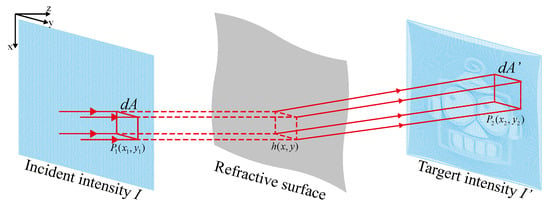
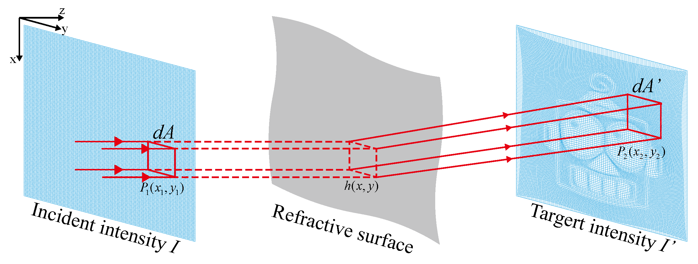
As illustrated in Figure 1, the incident beam propagates along the z-axis. The coordinates on the incident plane $P_1$ are denoted $x_1$ and $y_1$. The points on the target plane are described by $(x_2,y_2)$. Between the two planes is a refractive surface; it is a single value function z which is represented by x and y. To achieve the target distribution, we need to redistribute the incident beam’s energy according to the law of conservation. This process establishes a one-to-one mapping function between points on the incident plane and the target plane. For example, this implies that concentrating a bundle of light rays into a smaller spatial region increases the local flux density, whereas expanding the ray bundle results in a lower intensity. According to the energy conservation, we have

$$IdA=I^{\prime }d{A}^{\prime }$$

(1)

where I and $I^{\prime }$ represent the intensity distributions on the incident and target planes, respectively, while $dA$ and $d{A}^{\prime }$ denote the corresponding infinitesimal area elements. The coordinate transformation from the incident plane $(x_1,x_2)$ to the target plane $(x_1.x_2)$ is defined by the mapping function $x_2=f(x_1,y_1)$ and $y_2=g(x_1,y_1)$. By applying the conservation of energy to this mapping, we derive the Jacobian matrix:

$$J=\left[\begin{array}{cc}{\displaystyle \frac{\partial f}{\partial x_1}}& {\displaystyle \frac{\partial f}{\partial y_1}}\\ {\displaystyle \frac{\partial g}{\partial x_2}}& {\displaystyle \frac{\partial g}{\partial y_2}}\end{array}\right]$$

(2)

The determinant of the Jacobian matrix, $det\left(J\right)$, characterizes the local scaling ratio of an infinitesimal area element following the coordinate transformation. Consequently, the relationship is given by

$$I^{\prime }=det\left(J\right)I$$

(3)

Assuming a collimated uniform incident beam is incident into a uniform grid, the energy flux through each grid cell is identical. However, if the target plane is similarly discretized into a uniform grid, the energy within each cell will typically differ from that of the incident plane due to the non-uniform intensity distribution of the target field. To satisfy the energy conservation condition in Equation (3), the coordinates on the target plane must be adjusted. We introduced an error function, $E(x,y)$, to quantify the deviation between the transformed incident energy and the desired target energy distribution:

$$E(x,y)=Idet\left(J\right)-I^{\prime }$$

(4)

where E represents the local energy density residual. To minimize this error, the coordinate points $(x_2,y_2)$ on the target plane must be moved to locally expand or compress the grid cells. We model this process by treating the error E as a source term that drives the grid deformation, governed by the Poisson equation:

$${\nabla }^2\varphi =-E$$

(5)

where the scalar potential $\varphi$ defines a gradient field indicating the direction and magnitude of the required coordinate displacement. Once the gradient direction is determined, we introduce a virtual step t, which represents the displacement magnitude of the target plane coordinates along this gradient. The evolution of the coordinates is described by

$${\displaystyle \frac{\partial P_2}{\partial t}}=\nabla \varphi$$

(6)

This equation induces a slight deformation of the target grid, resulting in a new coordinate distribution. The updated coordinates are then substituted back into Equation (4) to recalculate the error. Generally, repeating this process for several iterations yields a stable energy mapping function from the incident plane to the target plane.

Following the determination of the mapping function, we proceed to calculate the refractive surface profile. We assume the incident beam propagates along the positive z-axis, corresponding to a unit incident vector $\widehat{\mathbf{I}}=(0,0,1)$. The surface sag is defined by $z=h(x,y)$. After refraction, the unit outgoing vector $\widehat{T}$ is expressed as

$$\widehat{\mathbf{T}}={\displaystyle \frac{\left(x_2-x_1,y_2-y_1,H-h(x,y)\right)}{\sqrt{{(x_2-x_1)}^2+{(y_2-y_1)}^2+{\left(H-h(x,y)\right)}^2}}}$$

(7)

where H denotes the axial position of the target plane. For brevity, we define the distance $d=\sqrt{{(x_2-x_1)}^2+{(y_2-y_1)}^2+{(H-h)}^2}$ to simplify Equation (7). The unit normal vector N of the refractive surface is given by

$$\mathbf{N}=\left({\displaystyle \frac{\partial h}{\partial x}},{\displaystyle \frac{\partial h}{\partial y}},-1\right)$$

(8)

Applying Snell’s law in vector form yields the relationship between the surface gradients and the coordinate mapping:

$$\left\{\begin{array}{cc}\hfill N_x& ={\displaystyle \frac{x_2-x_1}{d\left(n-\frac{H-h}{d}\right)}}\hfill \\ \hfill N_y& ={\displaystyle \frac{y_2-y_1}{d\left(n-\frac{H-h}{d}\right)}}\hfill \end{array}\right.$$

(9)

Subsequently, the surface height reconstruction is formulated as a Poisson equation:

$${\nabla }^{2}h=\nabla ·{\mathbf{N}}_{xy}$$

(10)

By solving Equation (10), we obtain the refractive surface height. The thin-element approximation is used to convert the refractive surface into the initial phase $\varphi (x,y)$:

$$\varphi (x,y)={\displaystyle \frac{2\pi }{\lambda }}(n-1)h(x,y)$$

(11)

where $\lambda$ is the wavelength of the light, and n is the refractive index of the material.

2.2. Stochastic Gradient Descent Principle

Through the calculations described above, the freeform surface is converted into a phase-only profile, which serves as the initialization for the SGD algorithm. During this optimization process, the angular spectrum method (ASM) is used as a diffraction propagation method to calculate the reconstructed distribution on the target plane. The expression of ASM is given by the following equation:

$$E_{\mathrm{ASM}}^{\mathrm{img}}\left(\varphi (x,y)\right)=\int \int E_{0}exp\left(j\varphi (x,y)\right)H(f_x,f_y)exp\left(j2\pi (f_{x}x+f_{y}y)\right)d{f}_{x}d{f}_y$$

(12)

where $\varphi (x,y)$ is the loaded phase value, $E_0$ is the incident filed amplitude, and $f_x$ and $f_y$ are the spatial frequency on the x and y axis. $E_{\mathrm{ASM}}^{\mathrm{img}}\left(\varphi (x,y)\right)$ is the reconstructed field distribution on the target plane. H is the transfer function in free space propagation, and it is written as

$$H(f_x,f_y)=exp\left(j{\displaystyle \frac{2\pi z}{\lambda }}\sqrt{1-{\left(\lambda f_x\right)}^2-{\left(\lambda f_y\right)}^2}\right)$$

(13)

where z is the light propagation distance between the hologram and the target plane. The reconstructed field distribution is expressed by $I_{\mathrm{ASM}}={\left|E_{\mathrm{ASM}}^{\mathrm{img}}\right|}^2=E_{\mathrm{ASM}}^{\mathrm{img}}·\overline{E_{\mathrm{ASM}}^{\mathrm{img}}}$. The loss function between the reconstructed field distribution and the desired distribution $I_{t}ar$ is shown as

$$L\left(\varphi \right)=\sum {\left(I_{\mathrm{ASM}}-I_{\mathrm{tar}}\right)}^2$$

(14)

Since the optical field distribution on the target plane is a complex amplitude, minimizing the loss function requires computing its gradient with respect to the propagated field $E_{ASM}$. Applying the chain rule, we derive the gradient expression:

$$g\left(\varphi \right)={\displaystyle \frac{\partial L\left(\varphi \right)}{\partial E_{\mathrm{ASM}}^{\mathrm{img}}}}={\displaystyle \frac{\partial L\left(\varphi \right)}{\partial I_{\mathrm{ASM}}}}{\displaystyle \frac{\partial I_{\mathrm{ASM}}}{\partial E_{\mathrm{ASM}}^{\mathrm{img}}}}$$

(15)

This equation calculates the gradient on the image plane, which quantifies how variations in the reconstructed field distribution influence the loss function. However, to update the hologram, it is necessary to determine the impact of the object plane phase profile on the loss function. Consequently, back propagation is required to map this error gradient from the image plane back to the object plane. The gradient on the object plane is expressed by

$$G\left(\varphi \right)=\int \int g\left(\varphi \right)exp\left(-j{\displaystyle \frac{2\pi z}{\lambda }}\sqrt{1-{\left(\lambda f_x\right)}^2-{\left(\lambda f_y\right)}^2}\right)exp\left(-j2\pi (f_{x}x+f_{y}y)\right)d{f}_{x}d{f}_y$$

(16)

By solving this equation, we obtain the gradient of the loss function with respect to the complex amplitude at the object plane; we now derive the gradient with respect to the phase profile. The relationship is given by

$${\displaystyle \frac{\partial L\left(\varphi \right)}{\partial \varphi }}=G\left(\varphi \right){\displaystyle \frac{\partial E_{\mathrm{ASM}}^{\mathrm{obj}}}{\partial \varphi }}$$

(17)

To ensure stable minimization of the loss function with respect to the phase of the hologram, we employ the Adaptive Moment with Maximal Second Moment algorithm (AMSrad) for iterative updates. AMSGrad improves upon standard optimization methods by maintaining an element-wise upper bound of the second moment bias correction. This mechanism prevents the effective step size from increasing unexpectedly during iterations, thereby enhancing convergence stability for non-convex optimization problems. Let $g_t={\displaystyle \frac{\partial L}{\partial {\varphi }_t}}$ denote the phase gradient at the t-th iteration. The exponential moving averages of the first and second moments of the gradient are calculated as follows:

$$\left\{\begin{array}{cc}\hfill m_t& ={\beta }_1{m}_{t-1}+(1-{\beta }_1)g_t\hfill \\ \hfill v_t& ={\beta }_2{v}_{t-1}+(1-{\beta }_2)g_t^2\hfill \end{array}\right.$$

(18)

where ${\beta }_1,{\beta }_2\in (0,1)$ represent the decay rates for the first moment and second moment estimates, respectively. To mitigate initialization bias, the following bias correction steps are performed:

$${\widehat{m}}_t={\displaystyle \frac{m_t}{1-{\beta }_1^t}},{\widehat{v}}_t={\displaystyle \frac{v_t}{1-{\beta }_2^t}}$$

(19)

Subsequently, a maximum value constraint is applied to the second moment estimate, ${\widehat{v}}_t^{max}=max\left({\widehat{v}}_{t-1}^{max},{\widehat{v}}_t\right)$. This step normalizes the update size using the historical maximum, effectively preventing increases in step size caused by a diminishing denominator. Finally, the updated phase is expressed as

$${\varphi }_{t+1}^{\prime }={\varphi }_t-\gamma \left(\alpha -{\displaystyle \frac{{\widehat{m}}_t}{\sqrt{{\widehat{v}}_t^{max}}+\epsilon }}\right)$$

(20)

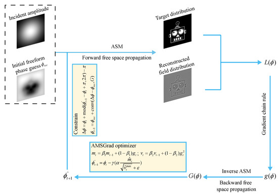
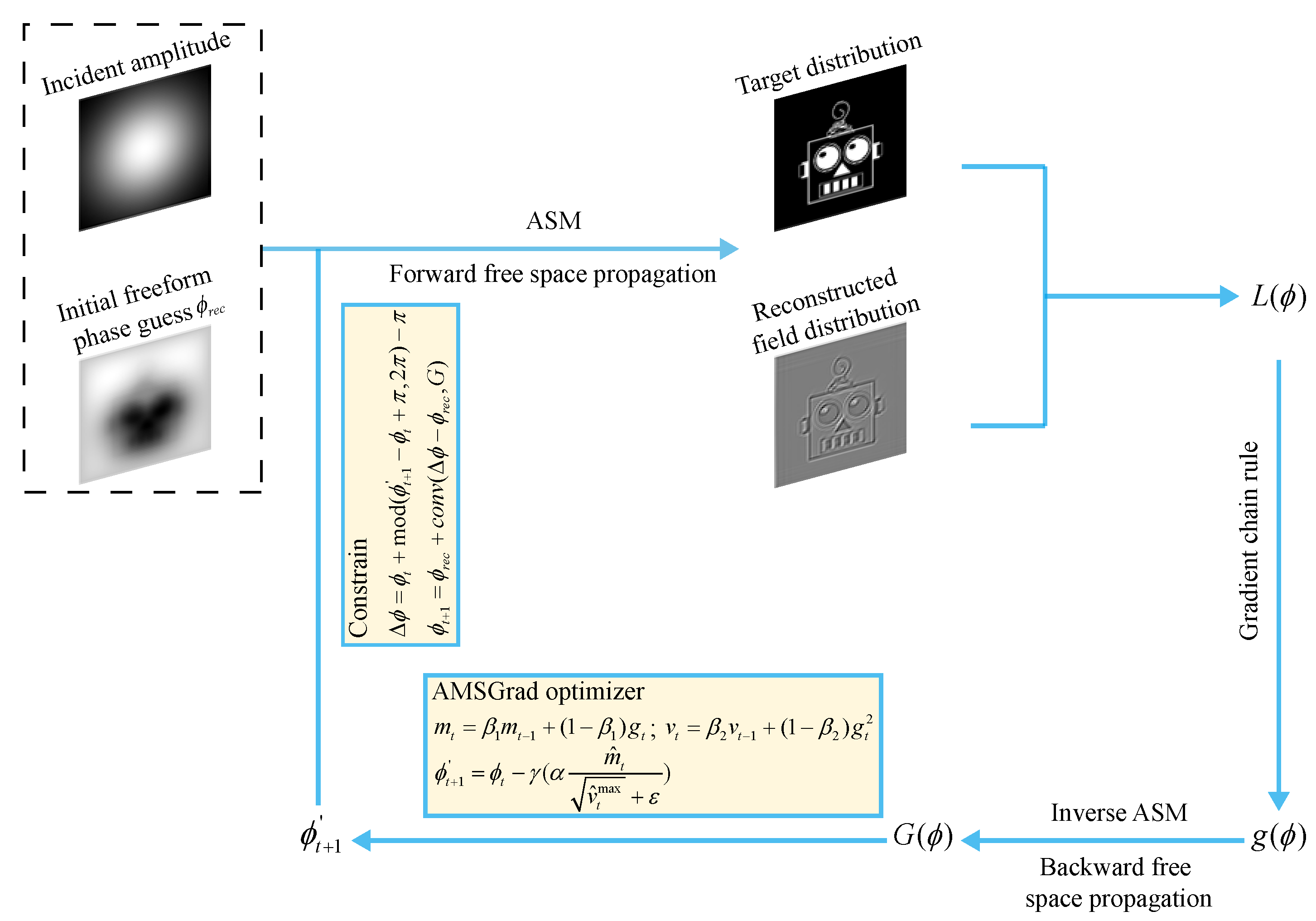
where $\alpha$ denotes the learning rate, and $\epsilon$ is a small constant added for numerical stability to prevent division by zero. The parameter $\gamma$ represents the step size factor, which varies with the iteration count. Since the specific choice of step size directly impacts both the convergence of the SGD algorithm and the reconstruction quality of the CGH, a detailed discussion is presented in the next section. Furthermore, phase constraints are incorporated into the SGD algorithm to prevent the optimized phase profile from deviating significantly from the smooth and continuous geometric initialization, as illustrated in Figure 2. At the end of each iteration, the phase difference between the updated phse and the previous phase is calculated using $\Delta \varphi ={\varphi }_t+mod\left({\varphi }_{t+1}^{\prime }-{\varphi }_t+\pi ,2\pi \right)-\pi$. This operation constrains the phase difference within the interval $[-\pi ,\pi ]$, effectively suppressing large phase jumps and preventing abrupt transitions. Then, we calculate the deviation between the updated phase and the geometrically derived initial phase, applying a Gaussian filter to the result. The introduction of this Gaussian kernel serves to smooth high-frequency nosie and suppress speckle effects, ensuring a continuous phase update. The final updated phase is expressed as ${\varphi }_{t+1}={\varphi }_{rec}+conv(\mathrm{\Delta }\varphi -{\varphi }_{rec},G)$. By repeating this iterative process, we ultimately obtain the optimized phase distribution capable of accurately reconstructing the desired optical field.

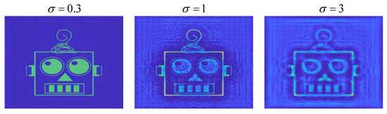
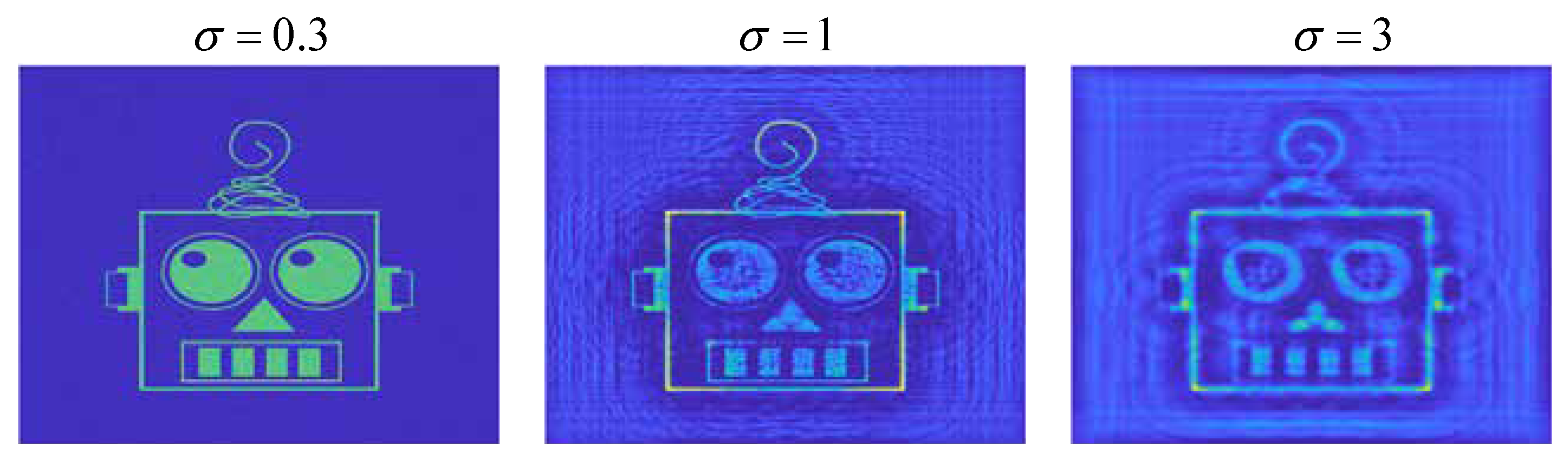
The diffraction reconstructions in Figure 3 illustrate the trade-off between phase profile smoothing and effective étendue, as controlled by the Gaussian kernel size. With a small kernel ($\sigma =0.3$), the phase retains more high spatial frequency content, so the reconstructed field preserves sharper edges and finer features of the target, consistent with a broader synthesized angular spectrum and better utilization of the SLM bandwidth. Increasing the smoothing to $\sigma =1$, the image becomes worse, fine structures are partially washed out, and the reconstruction shows more pronounced low-frequency background modulation. When the kernel is further enlarged ($\sigma =3$), most high-frequency information is suppressed, and it leads to a strong loss of detail, reduced contrast, and an overall blurred reconstruction. In other words, stronger phase smoothing improves phase continuity, but it narrows the effective spatial frequency support of the hologram and degrades reconstruction fidelity, which is especially detrimental for high-detail operation.

2.3. Objective Metrics

To evaluate the quality of the reconstructed image, we employ the structural similarity index measure (SSIM) and peak signal-to-noise ratio (PSNR) as objective metrics [31,32]. Given the intensity value $I_{A}SM$ in the reconstructed image and the intensity value $I_{t}ar$ in the desired image, the SSIM is defined as

$$\mathrm{SSIM}(I_{\mathrm{ASM}},I_{\mathrm{tar}})={\displaystyle \frac{(2{\mu }_x{\mu }_y+c_1)(2{\sigma }_{xy}+c_2)}{({\mu }_x^2+{\mu }_y^2+c_1)({\sigma }_x^2+{\sigma }_y^2+c_2)}}$$

(21)

where ${\mu }_x$ and ${\mu }_y$ are the average values of the intensity $I_{ASM}$ and $I_{tar}$, and ${\sigma }_x$ and ${\sigma }_y$ are the variances of the intensity; ${\sigma }_{xy}$ is the sample covariance, and $c_1$ and $c_2$ are small constants that prevent instability when denominators are near zero. The SSIM value considers changes in structural information, luminance, contrast, and texture, and its value lies in $[-1,1]$, with larger values indicating closer similarity. The PSNR presents the error on a logarithmic scale:

$$\mathrm{PSNR}=10·{log}_{10}\left({\displaystyle \frac{MA{X}_{\mathrm{val}}^2}{\mathrm{MSE}}}\right)$$

(22)

where $MA{X}_{val}$ is the maximum pixel value of the reconstructed image, and $MSE$ denotes the mean squared error between the constructed and original pixel values.

3. Experimental Results and Discussion

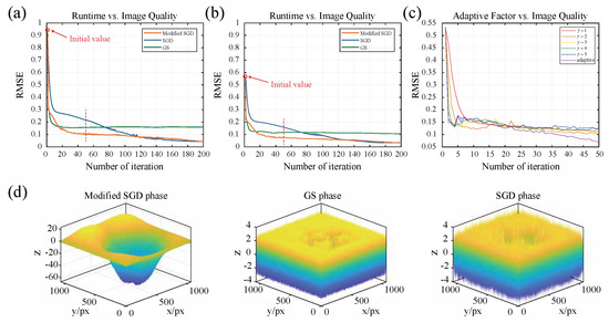
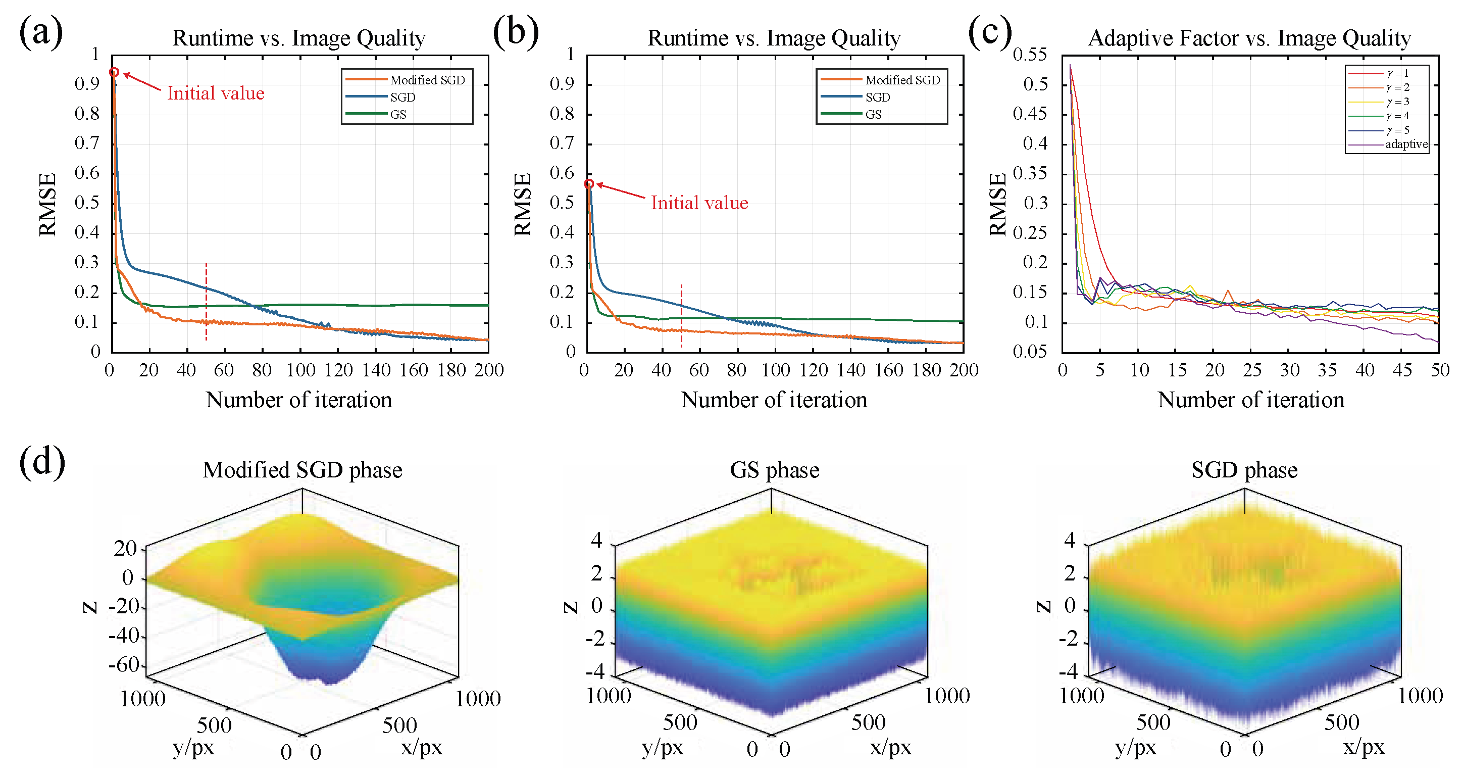
We compare the iterative performance and final phase distributions of the GS algorithm, the standard SGD algorithm, and our proposed modified SGD algorithm. These comparisons are illustrated in Figure 4.

Figure 4a compares the convergence performance of the modified SGD, standard SGD and GS algorithms for CGH optimizations. When the CGH iteration starts from a flat phase ($\varphi =0$), the initial reconstructed field is usually far from the desired target. As a result, the early iterations spend more iteration on calculating the correct spatial frequency content, so the RMSE value begins at a relatively large value and decreases more gradually. In contrast, using a calculated smooth phase as the starting point provides a much better initialization, as shown in Figure 4b. This is because the smooth phase already encodes an approximation of the target wavefront, and the initial reconstruction is closer to the desired image. Therefore, all three algorithms begin with a smaller initial error and present a faster drop in the error curve in the iteration process. In both Figure 4a,b, the modified SGD algorithm and GS algorithm exhibit nearly identical convergence rates, indicating comparable optimization speed. However, the GS algorithm converges to a higher RMSE value, suggesting that it reaches a suboptimal solution with limited reconstruction accuracy. In contrast, the modified SGD algorithm achieves a final reconstruction quality comparable to standard SGD while maintaining GS-like convergence speed. These results indicate that the modified SGD algorithm preserves the high-quality reconstruction of SGD but significantly accelerates convergence, effectively combining the strengths of both methods. Figure 4c investigates the impact of different factor values on the convergence efficiency and image quality. When $\gamma$ is set to 1, the algorithm exhibits a slower convergence rate, resulting in a suboptimal final RMSE after 50 iterations. Increasing the factor ($\gamma =2,3$) accelerates the descent speed, and the error is further reduced. However, as $\gamma$ is increased to 4 or 5, the initial convergence is rapid, but the excessive step size results in a higher RMSE. To address this, we implemented a dynamic adaptive factor that decreases as iterations progress. As shown by the purple curve, this approach achieves an initial convergence speed comparable to the $\gamma =5$ setting, yet it stabilizes at the lowest RMSE. Therefore, by dynamically adjusting the adaptive factor, the proposed method effectively balances rapid convergence with high-precision reconstruction, avoiding the pitfalls of fixed step sizes. Figure 4d illustrates the final optimized phase maps for the three algorithms. Compared with the other two final phase maps, the phase map optimized by the modified SGD maintains the smooth and continues characteristics of the initial refractive surface. This preservation can reduce phase abruptions and discontinuities, which is important for suppressing noise and stray light in the reconstructed image. In contrast, the phase maps generated by the standard SGD and GS algorithms exhibit more high-frequency noise and transitions.

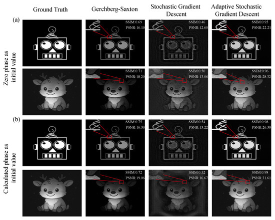
Then, we present the simulated results for two distinct examples; one is a binary amplitude image, and the other is a grayscale continuous image, as shown in Figure 5. Specifically, Figure 5a presents the results when all algorithms start from a zero phase initialization, whereas Figure 5b reports the results when all algorithms start from the calculated initial phase derived from the refractive surface. In both groups, all methods are run under the 50 iterations. It can be observed that the standard SGD algorithm fails to converge effectively within the limited time and exhibits significant deviation from the ground truth. The GS algorithm manages to stabilize within 50 iterations, and its reconstruction quality is inferior to the proposed method. According to the zoomed-in regions, the GS results are degraded by visible noise artifacts and speckle. However, the adaptive SGD reaches a stable solution and achieves consistently higher SSIM and PSNR than GS and standard SGD. Moreover, by comparing results shown in Figure 5a,b, we find that using the calculated refractive surface phase for initialization improves the reconstruction metrics for all three algorithms to different extents.

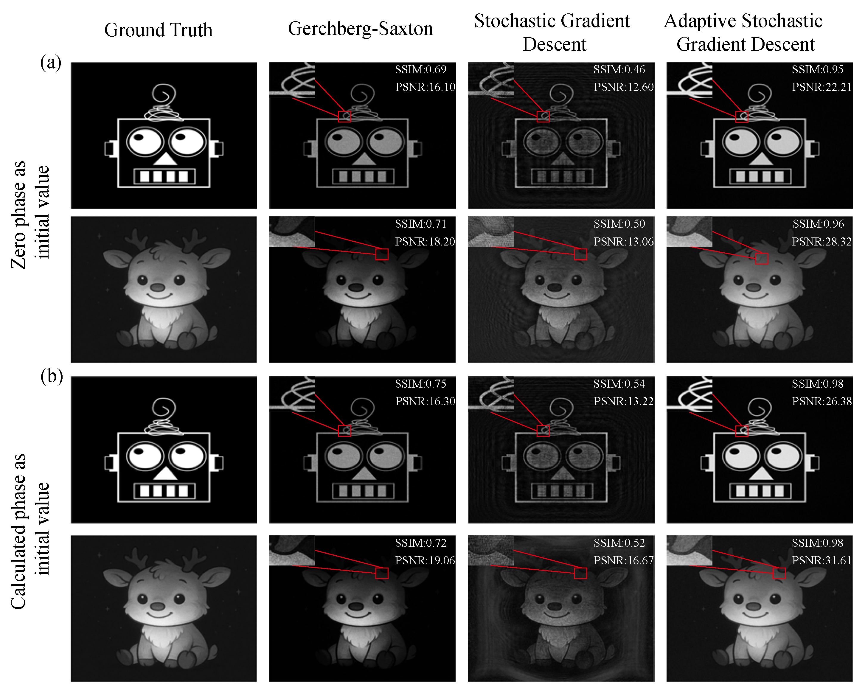
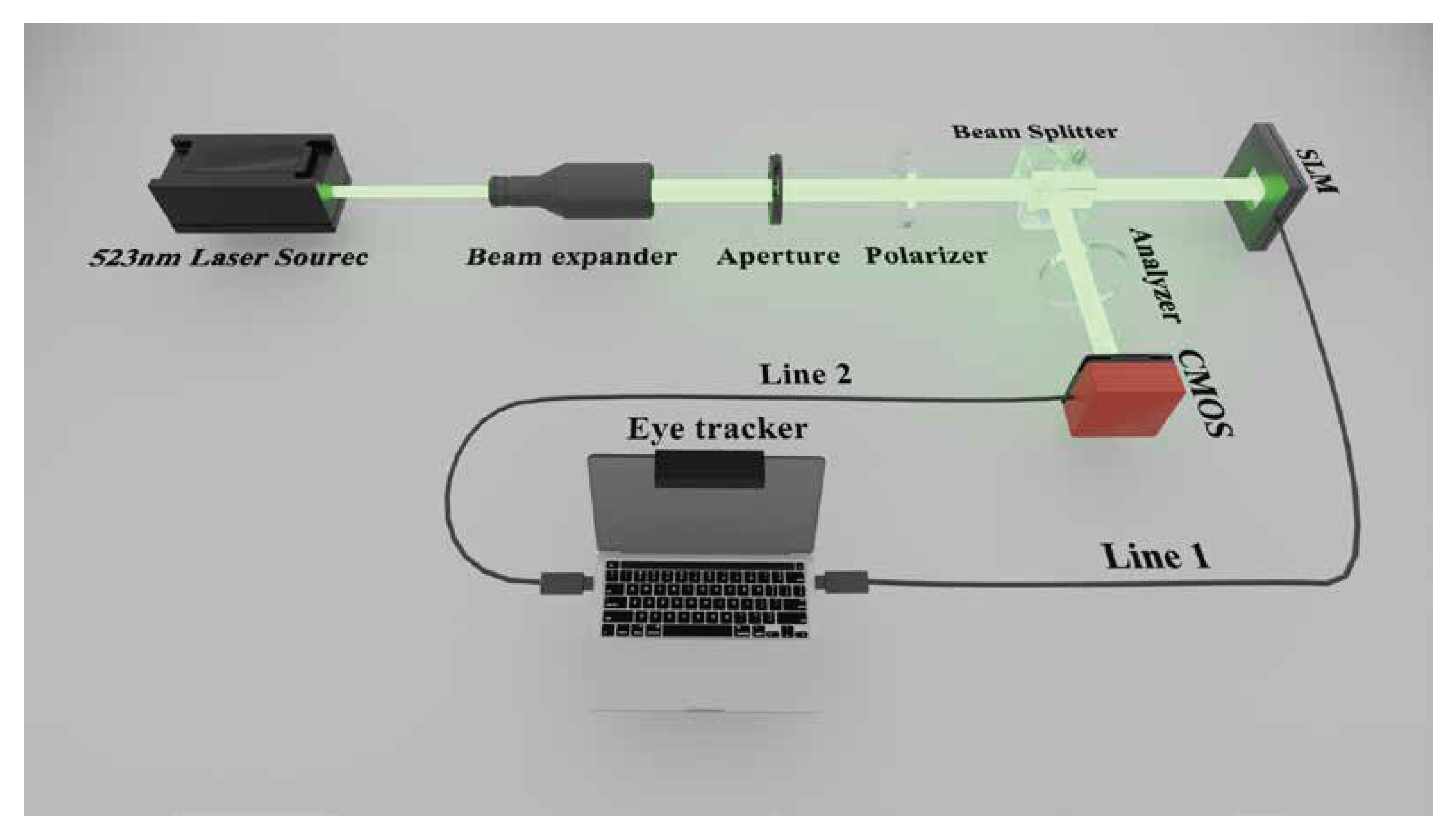
Finally, the proposed method is used in an autofocusing holographic system. The optical schematic is illustrated in Figure 6. The 532 nm laser serves as the coherent light source. The beam is initially expanded and collimated by a beam expander to ensure uniform illumination. An aperture is used to control the size of the beam, so the spot fits the SLM’s active area. A polarizer is used to set the polarization of the incident beam, since only the polarization component aligned with the SLM’s working axis can be effectively modulated. The polarized beam transmits through a beam splitter and illuminates the reflective SLM. The resolution is 1920 × 1080, and the pixel size is 6.4 um. The modulated wavefront is reflected back to the beam splitter and redirected toward a CMOS camera. Line 1 orders the SLM to load the optimized phase map, and Line 2 orders the CMOS to capture images. Furthermore, a Tobii X2-30 eye tracker is integrated into the system to detect the direction of the observer’s gaze, enabling real-time gaze-contingent autofocusing.

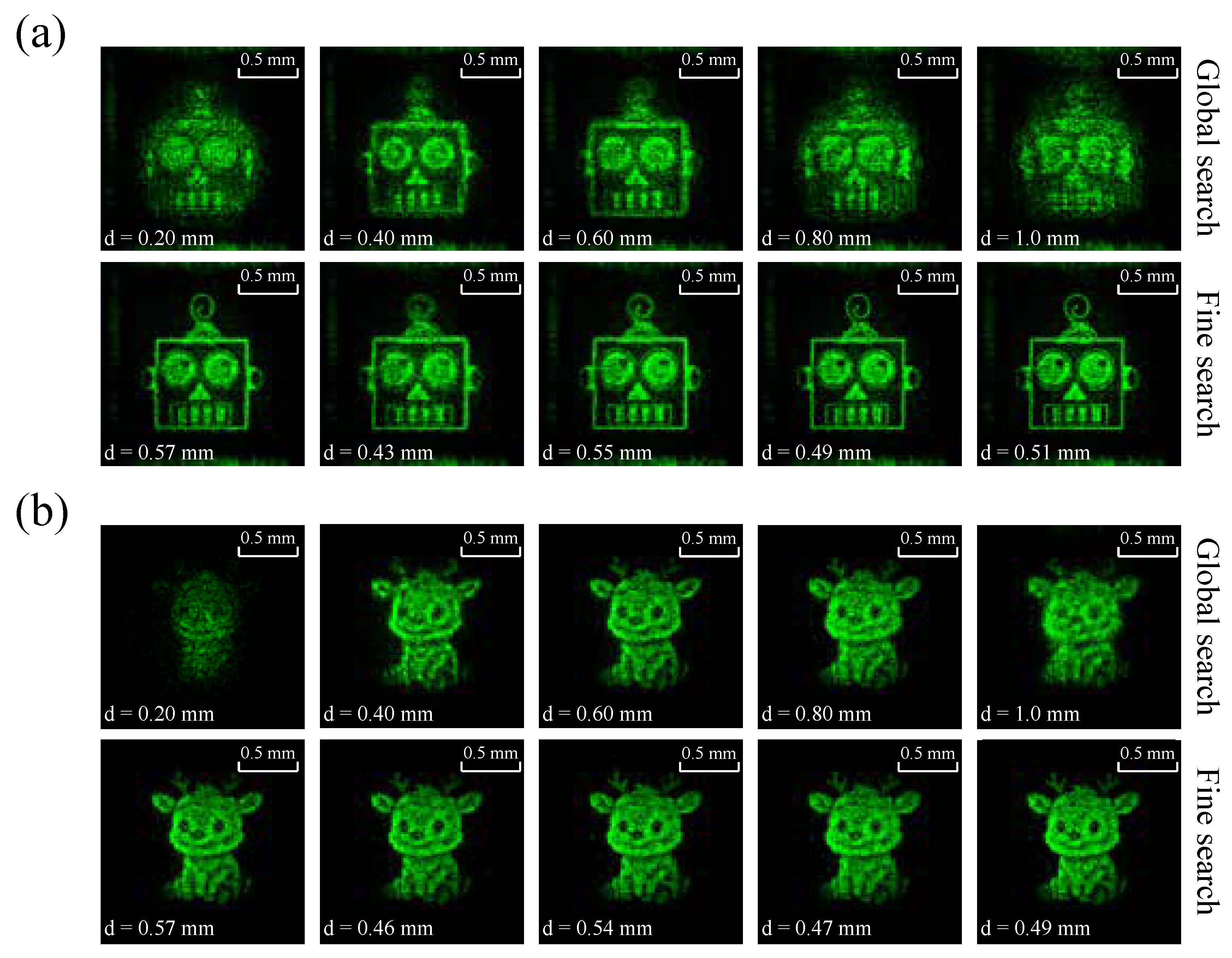
The autofocus procedure is detailed in Algorithm 1. To efficiently locate the optimal focal length within the range $d_{min},d_{max}$ while minimizing the number of iterations, we employ a hybrid strategy combining a global coarse search with a fine search based on parabolic interpolation. Initially, the global coarse search scans the designated range to identify the discrete focal length, which yields the highest PSNR value. Subsequently, a fine search is initialized around this current estimate using three adjacent focal points. These measurements are fitted to a second-order polynomial. By analyzing the polynomial coefficients $(a,b,c)$, the algorithm determines the curve; if the parabola is concave, its vertex $f_{new}=-b/2\ast a$ provides a continuous estimate of the focal length that maximizes the PSNR. Conversely, if the fit is not concave, the algorithm falls back to the best of the three discrete sampled points. This interpolation process is repeated for several iterations to ensure convergence to the precise optimal focus value.

Algorithm 1: Autofocus program

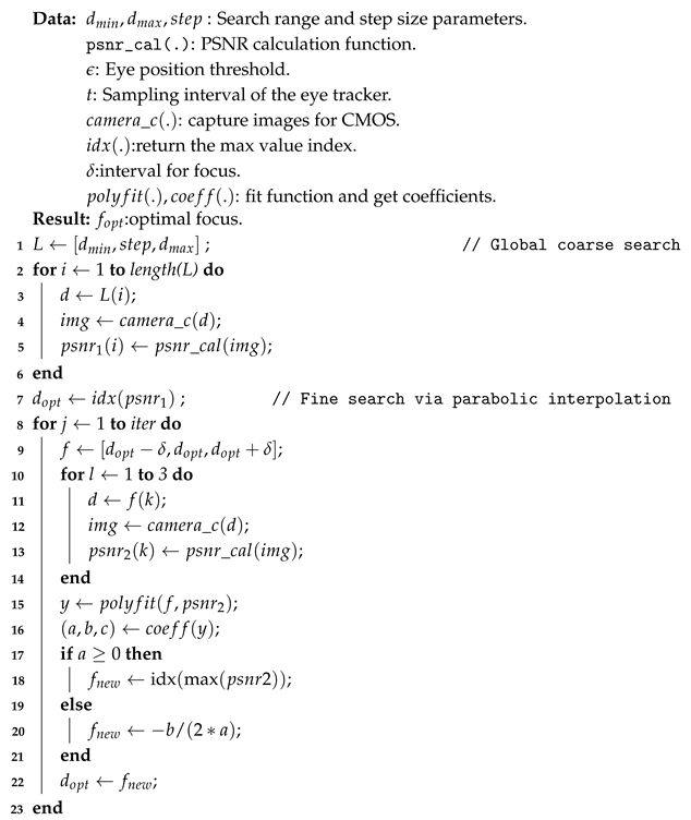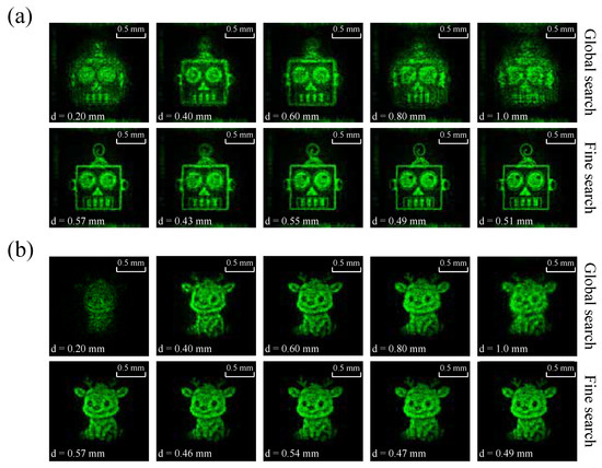
Figure 7 demonstrates the two-step autofocus results for two images. The camera is fixed at a distance of 0.5 m to capture the holographic reconstructions. The autofocusing system’s process is divided into two distinct stages according to Algorithm 1. The system first scans a wide range of focus from 0.2 m to 1.0 m. In the first row in Figure 7a, at d = 0.20 m and d = 1.0 m, the images are significantly defocused and blurry with low contrast. The visual quality improves as the distance approaches the center. The system identifies the optimal focal position from 0.40 m to 0.60 m. Then, the system switches to a fine search algorithm and converges effectively, determining the optimal focus parameter (d = 0.51 m). The final image has high contrast and clear edges, indicating that the phase map loaded onto the SLM matches the camera position. In Figure 7b, the system also yields the sharpest reconstructions.

4. Conclusions

In this study, we present an autofocus system based on an eye tracker device. By combining the advantages of refractive and diffractive beam shaping, we calculate a good start point for the CGH algorithm. We refine the SGD algorithm and introduce an adaptive step factor to increase the calculation efficiency. Compared to the standard SGD algorithm, the modified SGD algorithm exhibits four times higher computational efficiency. Furthermore, due to the constraints of the modified SGD algorithm, the smoothness of the diffractive surface profile reduces noise in the reconstructed field. The effectiveness of our proposed method is demonstrated herein by simulation and experimental results. The system finally calculates the optimal focus of the phase map. We hope that the eye tracker-based autofocus system will contribute to AR/VR technologies.

References

- Grier, D.G.; Roichman, Y. Holographic optical trapping. Appl. Opt. 2006, 45, 880–887. [Google Scholar] [CrossRef] [Scilit]
- Woerdemann, M.; Alpmann, C.; Esseling, M.; Denz, C. Advanced optical trapping by complex beam shaping. Laser Photonics Rev. 2013, 7, 839–854. [Google Scholar] [CrossRef] [Scilit]
- Yuan, G.; Zhou, M.; Peng, Y.; Chen, M.; Geng, Z. Error-compensation network for ringing artifact reduction in holographic displays. Opt. Lett. 2024, 49, 3210–3213. [Google Scholar] [CrossRef] [Scilit]
- Liu, T.; Ning, H.; Cao, H.; Luo, D.; Xu, Z.; Luo, C.; Su, G.; Liu, Y.; Yao, R.; Peng, J. Research progress of large viewing-area 3D holographic near-eye display. Laser Photonics Rev. 2024, 18, 2300641. [Google Scholar] [CrossRef] [Scilit]
- He, L.; Chen, X.; Yang, Y.; Liu, X.; Chen, Y.; Xu, L.; Gu, C. Using high-diffraction-efficiency holographic optical elements in a full-color augmented reality display system. Opt. Express 2023, 31, 29843–29858. [Google Scholar] [CrossRef] [Scilit]
- Rosen, J.; Brooker, G. Non-scanning motionless fluorescence three-dimensional holographic microscopy. Nat. Photonics 2008, 2, 190–195. [Google Scholar] [CrossRef] [Scilit]
- O’Connor, T.; Doblas, A.; Javidi, B. Structured illumination in compact and field-portable 3D-printed shearing digital holographic microscopy for resolution enhancement. Opt. Lett. 2019, 44, 2326–2329. [Google Scholar] [CrossRef] [Scilit]
- Peng, Y.; Choi, S.; Padmanaban, N.; Wetzstein, G. Neural holography with camera-in-the-loop training. ACM Trans. Graph. 2020, 39, 1–14. [Google Scholar] [CrossRef] [Scilit]
- Gabor, D. Holography, 1948–1971. Science 1972, 177, 299–313. [Google Scholar] [CrossRef] [Scilit]
- Pi, D.; Liu, J.; Wang, Y. Review of computer-generated hologram algorithms for color dynamic holographic three-dimensional display. Light Sci. Appl. 2022, 11, 231. [Google Scholar] [CrossRef] [Scilit] [PubMed]
- Zhang, H.; Zhao, Y.; Cao, L.; Jin, G. Fully computed holographic stereogram based algorithm for computer-generated holograms with accurate depth cues. Opt. Express 2015, 23, 3901–3913. [Google Scholar] [CrossRef] [Scilit] [PubMed]
- Madsen, A.E.G.; Eriksen, R.L.; Glückstad, J. Comparison of state-of-the-art computer generated holography algorithms and a machine learning approach. Opt. Commun. 2022, 505, 127590. [Google Scholar] [CrossRef] [Scilit]
- Blinder, D.; Nishitsuji, T.; Schelkens, P. Real-time computation of 3D wireframes in computer-generated holography. IEEE Trans. Image Process. 2021, 30, 9418–9428. [Google Scholar] [CrossRef] [Scilit]
- Sui, X.; He, Z.; Chu, D.; Cao, L. Non-convex optimization for inverse problem solving in computer-generated holography. Light Sci. Appl. 2024, 13, 158. [Google Scholar] [CrossRef] [Scilit]
- Yang, G.; Dong, B.; Gu, B.; Zhuang, J.Y.; Ersoy, O.K. Gerchberg–Saxton and Yang–Gu algorithms for phase retrieval in a nonunitary transform system: A comparison. Appl. Opt. 1994, 33, 209–218. [Google Scholar] [CrossRef] [Scilit]
- Hwang, H.E.; Chang, H.T.; Lie, W.N. Fast double-phase retrieval in Fresnel domain using modified Gerchberg-Saxton algorithm for lensless optical security systems. Opt. Express 2009, 17, 13700–13710. [Google Scholar] [CrossRef] [Scilit]
- Fienup, J.R. Phase retrieval algorithms: A comparison. Appl. Opt. 1982, 21, 2758–2769. [Google Scholar] [CrossRef] [Scilit]
- Chen, C.; Lee, B.; Li, N.N.; Chae, M.; Wang, D.; Wang, Q.H.; Lee, B. Multi-depth hologram generation using stochastic gradient descent algorithm with complex loss function. Opt. Express 2021, 29, 15089–15103. [Google Scholar] [CrossRef] [Scilit] [PubMed]
- Shen, C.; Zheng, Y.; Le, Z. Novel approach based on stochastic gradient descent for controlling the reconstructed phase randomness of computer-generated holograms. Opt. Lasers Eng. 2023, 166, 107593. [Google Scholar] [CrossRef] [Scilit]
- Chen, Y.; Chi, Y.; Fan, J.; Ma, C. Gradient descent with random initialization: Fast global convergence for nonconvex phase retrieval. Math. Program. 2019, 176, 5–37. [Google Scholar] [CrossRef] [Scilit] [PubMed]
- Chakravarthula, P.; Peng, Y.; Kollin, J.; Fuchs, H.; Heide, F. Wirtinger holography for near-eye displays. ACM Trans. Graph. 2019, 38, 1–13. [Google Scholar] [CrossRef] [Scilit]
- Schroff, P.; La Rooij, A.; Haller, E.; Kuhr, S. Accurate holographic light potentials using pixel crosstalk modelling. Sci. Rep. 2023, 13, 3252. [Google Scholar] [CrossRef] [Scilit] [PubMed]
- Wu, R.; Wang, H.; Liu, P.; Zhang, Y.; Zheng, Z.; Li, H.; Liu, X. Efficient optimal design of smooth optical freeform surfaces using ray targeting. Opt. Commun. 2013, 300, 100–107. [Google Scholar] [CrossRef] [Scilit]
- Ries, H.; Muschaweck, J. Tailored freeform optical surfaces. J. Opt. Soc. Am. A 2002, 19, 590–595. [Google Scholar] [CrossRef] [Scilit]
- Schmidt, S.; Thiele, S.; Toulouse, A.; Bösel, C.; Tiess, T.; Herkommer, A.; Gross, H.; Giessen, H. Tailored micro-optical freeform holograms for integrated complex beam shaping. Optica 2020, 7, 1279–1286. [Google Scholar] [CrossRef] [Scilit]
- Doskolovich, L.L.; Mingazov, A.A.; Byzov, E.V.; Skidanov, R.V.; Ganchevskaya, S.V.; Bykov, D.A.; Bezus, E.A.; Podlipnov, V.V.; Porfirev, A.P.; Kazanskiy, N.L. Hybrid design of diffractive optical elements for optical beam shaping. Opt. Express 2021, 29, 31875–31890. [Google Scholar] [CrossRef] [Scilit]
- Feng, Z.; Froese, B.D.; Liang, R. Composite method for precise freeform optical beam shaping. Appl. Opt. 2015, 54, 9364–9369. [Google Scholar] [CrossRef] [Scilit] [PubMed]
- Shi, L.; Li, B.; Kim, C.; Kellnhofer, P.; Matusik, W. Towards real-time photorealistic 3D holography with deep neural networks. Nature 2021, 591, 234–239. [Google Scholar] [CrossRef] [Scilit] [PubMed]
- Choi, S.; Gopakumar, M.; Peng, Y.; Kim, J.; O’Toole, M.; Wetzstein, G. Neural 3D holography: Learning accurate wave propagation models for 3D holographic virtual and augmented reality displays. ACM Trans. Graph. 2021, 40, 240. [Google Scholar] [CrossRef] [Scilit]
- Yue, Y.; Iwasaki, K.; Chen, B.Y.; Dobashi, Y.; Nishita, T. Poisson-based continuous surface generation for goal-based caustics. ACM Trans. Graph. 2014, 33, 1–7. [Google Scholar] [CrossRef] [Scilit]
- Brunet, D.; Vrscay, E.R.; Wang, Z. On the mathematical properties of the structural similarity index. IEEE Trans. Image Process. 2012, 21, 1488–1499. [Google Scholar] [CrossRef] [Scilit] [PubMed]
- Setiadi, D.R.I.M. PSNR vs SSIM: Imperceptibility quality assessment for image steganography. Multimed. Tools Appl. 2021, 80, 8423–8444. [Google Scholar] [CrossRef] [Scilit]
Disclaimer/Publisher’s Note: The statements, opinions and data contained in all publications are solely those of the individual author(s) and contributor(s) and not of MDPI and/or the editor(s). MDPI and/or the editor(s) disclaim responsibility for any injury to people or property resulting from any ideas, methods, instructions or products referred to in the content. |
© 2026 by the authors. Licensee MDPI, Basel, Switzerland. This article is an open access article distributed under the terms and conditions of the Creative Commons Attribution (CC BY) license.