


Abstract
Regenerative vibrations are a major hindrance to flexible cantilever structures during milling, resulting in a reduced tool life and diminished surface finish. In this research, two actively controlled methods are directly compared: a genetic algorithm (GA)-optimized classical proportional-integral-derivative (PID) controller and a GA-optimized fractional-order PID (FOPID) controller for a milling-dependent regenerative force on a flexible cantilever beam via numerical modeling, using piezoelectric actuator/sensor patches. The original aspect lies in synergistically combining fractional-order control with genetic algorithm-based optimization to actively reduce chatter and increase the machining stability of flexible milling systems. The simulation results from the GA-FOPID controller exhibited a reduction in vibration of approximately 92.70% compared with the open-loop system by reducing the RMS value from 1.5058 × 10⁻⁴ m to 1.0996 × 10⁻⁵ m. By reducing the vibration level and enlarging the predicted stable machining region, these improvements could potentially contribute to longer tool life, improved surface finish, and reduced post-processing requirements, although these technological benefits were not directly modeled in the present study. The main innovation of this work involves a unique combination of fractional-order control, PZT actuation, and genetic algorithm optimization in a regenerative milling delay architecture. To the best of the authors’ knowledge, based on the literature surveyed in this work, this combination of techniques has not previously been reported for active chatter suppression. The stability lobe diagram (SLD) analysis, conducted under the single-mode approximation that serves as the reference framework for the like-for-like comparison of the five investigated configurations, shows that the critical axial depth of cut at the representative spindle speed increases from ap,crit(1500) = 0.061 mm for the uncontrolled system to 0.52 mm under GA-FOPID control. This enlargement of the predicted stable machining region was further confirmed, at a comparable order of magnitude, when the structural model was extended to include the two next bending modes, indicating that the trend is not an artifact of the single-mode simplification. Therefore, although the results were obtained exclusively from numerical simulation and have not yet been experimentally validated, they support the use of optimization-based methods to implement FOPID strategies as a means to increase both reliability and performance of flexible milling configurations.
Keywords:
cantilever beam; milling; chatter; active vibration control; PID; FOPID; genetic algorithm 1. Introduction
The aeronautical industries widely use high-speed milling of thin-walled components known for their low stiffness. However, self-excited vibrations called chatter originate from dynamic tool–workpiece interactions [1]. These regenerative vibrations manifest when the structural flexibility of the thin-walled workpiece induces a phase lag relative to the dynamic cutting forces, driving a self-excited feedback loop. Severe consequences include both substandard surface quality that generates visible marks and laborious manual finishing requirements. Moreover, chatter accelerates tool wear, increases cutting forces and reduces geometric accuracy, which increases production costs while decreasing process efficiency [2]. Understanding this phenomenon forms an essential step toward developing precision manufacturing techniques that predominantly support the manufacturing of high-performance lightweight components.
In milling operations, regenerative chatter prediction and suppression continue to be major difficulties due to the interactions between the forces created by the cutting process and the dynamics of the structure when working with flexible structures. These vibrations have a significant impact on the performance of machining processes, including stability, surface finish, and productivity. Therefore, a great deal of research has been conducted to develop methods to prevent vibrations, resulting in enhanced dynamic performance and reliability.
The increasing need for better manufacturing productivity has led researchers to develop passive and active vibration control strategies that fine-tune the machining process stability limits. Many passive methods are directly related to the operational part of the machine tool and have been shown to be simple, robust and effective in controlling machining vibration. Chaari et al. [3] carried out an experimental study on spherical ball impact dampers, demonstrating their great potential for reducing structural vibration levels. Similarly, Gafsi et al. [4] presented a passive absorber installed in the milling cutter spindle which was able to effectively suppress the structural modes causing regenerative chatter. Chaari et al. [5] showed that passive damping achieved vibration reduction as well as quality improvement (flatness) on a workpiece, which indicates that there is an obvious link between dynamic stability and surface finish.
Given the restrictions of totally passive solutions, efforts have also been devoted to developing active vibration control (AVC) strategies which influence the chatter stability boundaries of machining systems. Mechatronic systems are implemented to create dynamic forces that counteract and cancel structural vibrations. Actuators, sensors, and controllers are generally the main components of these systems used to maintain stable machining operations [1]. Model-based control methods, including Linear Quadratic Gaussian (LQG) and H-infinity (H∞) techniques, provide effectiveness in milling operation stabilization through utilization of system dynamic responses for parameter tuning [2]. Li et al. developed an intelligent strategy by combining an optimized Linear Quadratic Regulator (LQR) with an Adaptive Neuro-Fuzzy Inference System (ANFIS) to mitigate chatter [6]. In addition, to enhance system robustness, Van de Wouw et al. implemented a μ-synthesis-based controller design that successfully suppresses regenerative chatter under various machining conditions [7], while Paul and Morales-Menendez et al. [8] developed a hybrid control method merging PD/PID controllers with Type-2 Fuzzy Logic to compensate for system nonlinearities through fuzzy processing and thus improve control results. Such controllers are implemented for complex systems and designed to deal with dynamic nonlinear behaviors that exceed the PID capacity. These limitations have motivated the emergence of fractional-order controllers, which have attracted considerable interest over the last two decades due to their ability to handle complex system dynamics using fractional powers of integral and derivative terms [9]. Due to their additional tuning parameters, they have been successfully applied to regulate different manufacturing and engineering processes where they provide excellent performance, adaptability, and effectiveness [10,11]. Du et al. [12] discuss active chatter mitigation in machining using time-delay feedback control for vibration suppression.
Recent studies have established that fractional-order strategies possess unique capabilities for modeling and controlling complex dynamic plants. For instance, Ding et al. [13] developed an adaptive chatter-suppression approach that combines a fractional-order PID (FOPID) controller with spindle speed variation to broaden the stability region in milling operations.
Soufi et al. [14] developed a combination of Active Disturbance Rejection Control (ADRC) and Fractional-Order PID (FOPID) using Particle Swarm Optimization to tune out the effects of actuator saturation. The new method produced a 68.5% reduction in the RMS and greatly expanded the stability-lobe borders in the case of regenerative chatter control during milling processes involving electromagnetic proof-mass actuators.
In addition, compared to conventional control methodologies, the Jellyfish Search Optimizer (JSO)-based FOPID strategy offers a more robust and efficient approach for controlling paper machine headbox pressure and stock level, ensuring improved dynamic performance and stability [15].
Smart materials, specifically lead zirconate titanate (PZT) ceramics, possess reciprocal electromechanical properties that enable simultaneous vibration sensing and actuation. They function as sensors by generating electrical charge under mechanical deformation, and as actuators by inducing mechanical strain when subjected to an electric field [16]. PZT materials produce substantial actuation forces relative to their size. When bonded, deposited, or embedded into a structure, they minimally influence its weight and performance [17].
The performance of the control system and the controlled response depend heavily on where sensors and actuators are installed. Research on optimal placement represents a significant portion of studies on these components. Ongoing research continues to explore the promising capabilities of piezoelectric smart structures within engineering settings. For instance, through Euler–Bernoulli beam theory combined with PZT actuators and an LQR controller, Hashemi et al. [18] developed a smart active vibration control system for wind turbine blades to minimize the transverse vibrations and reduce bending deformation under external loads.
Fractional-order approaches have lately become quite popular because they provide a mathematically rigorous framework for modeling and controlling non-local complex systems characterized by hereditary behavior and memory effects. In machining operations, the occurrence of regenerative chatter and the structural coupling between the machine components result in time-varying behavior that cannot be easily described by conventional integer-order dynamic models. Therefore, several researchers have demonstrated that fractional-order approaches to modeling systems are significantly better than classical approaches for tracking performance and reducing vibration, and they also provide improved system representation. However, very little research has been conducted in the area of GA-optimized FOPID controller integration with smart PZT-enabled flexible machining systems while concurrently considering the regenerative delay dynamics and enhancing the stability lobes of the milling system. To the best of the authors’ knowledge, limited works have addressed GA-optimized FOPID active chatter suppression using collocated PZT actuation integrated with regenerative milling dynamics and stability-lobe analysis.
Previously established research in the area of active suppression of chatter in machining has addressed portions of the overall problem. FOPID control has been employed as a method to mitigate vibrations in cantilevered beam structures [9], during various manufacturing operations [13,14], and for PID controller tuning with genetic algorithms in various engineering applications [19,20]. In addition, both [6,8] provide examples of AI-assisted tuning of chatter controllers for milling. Robust μ-synthesis has been pursued using a model-based approach in [7]. Validation of collocated PZT actuation on flexible structures has occurred in [14] across controller type, optimization method, machining/application model, inclusion of the regenerative delay, validation method, and key findings.
Considering the limitations we have identified, the objective of this research is to identify and develop different methods of active vibration control for reducing vibrations that occur during milling operations. The first method utilizes a standard PID controller, while the second employs a FOPID controller. Both methods will be tuned using a GA, which is an artificial intelligence-based optimization method that provides optimal results compared with traditional tuning techniques. This paper demonstrates the advantages of evolutionary optimization techniques over conventional tuning techniques by improving parameter selection and overall dynamical performance of both controllers. This research enhances our understanding of vibration attenuation mechanisms while providing practical recommendations for improving the reliability of machining operations and suppressing chatter. We also conduct detailed comparisons between both control strategies in terms of their dynamic characteristics, their ability to reduce vibration, and their practical implementation to help in modeling more efficient and effective vibration reduction systems for flexible milling structures.
The remainder of this document is structured as follows. The mathematical modeling of the beam’s dynamic system is discussed in Section 2. A comprehensive description of the problem is given, along with a simplified dynamic scenario. A time-domain system model was established as the basis for the numerical investigation. Section 3 presents the PID and FOPID controllers along with their optimized control law versions based on a genetic algorithm (GA) method, and subsequently analyzes the stability of chatter. Next, the simulation, numerical results and frequency-domain analysis for the different approaches are shown together with a stability lobe diagram interpretation as well as an operational sensitivity analysis in Section 4. Finally, a comparative discussion of the control strategies’ performances is presented in Section 5 before the summary of main conclusions.
2. Mathematical Modeling
2.1. Milling Process Modelling
Modeling the cutting process is crucial for studying and suppressing the chatter phenomenon during milling operations, which involve an interaction between the workpiece and the cutting tool, as shown in Figure 1.
Figure 1.
Dynamics of the milling operation.
The cutting forces that excite the structure were introduced in [21] as simplified orthogonal cutting forces to model their dynamics during the manufacturing process. They are described as follows:
where Ftj and Frj denote, respectively, the tangential and radial cutting forces; Ktc and Krc are, respectively, the tangential and radial cutting coefficients; Kre and Kte are, respectively, the edge force coefficients; ap represents the depth of cut, and hj represents the instantaneous chip thickness.
The formulation proposed by Altintas [22] enables the calculation of the regenerative cutting force Fc at the tool tip acting on the flexible plate:
where Z is the number of cutter teeth, and φj represents the angular position of the j-th tooth.
As shown in Figure 2 above, hj(t) represents the chip cut thickness by tooth j, which depends on the tooth position y(t) at the instant t and the tooth position at the previous pass y (t − τ). Between two passes, a time interval τ, known as the time delay, has passed, and the tooth progresses by h0(t), corresponding to the parameter known as tooth feed. So, this leads to the following relationship:
where the engagement function is given as:
where φst and φex are, respectively, the immersion angles at the entry and exit states, and φj is the radial immersion angle, given by:
Figure 2.
Regenerative effects.
Half immersion milling conditions were used in this study; the radial immersion ratio was defined as ae/D = 0.5, and the cutter engagement was defined as an entry angle of φst = 0 and an exit angle of φex = π/2, corresponding to up milling.
In milling operations, the time delay is usually expressed as:
where N is the spindle speed.
The chip thickness expression can be expanded as follows:
where fz represents the feed per tooth (mm/tooth).
By substituting Equations (6) and (7) into Equation (2), the regenerative dynamic force becomes:
With
Thus, for all teeth engaged, the expression of becomes:
For a rectangular cantilever beam, the expression for bending stiffness is written as:
The directional stiffness ratio is derived as follows:
where
Therefore,
Therefore, since the beam’s geometry has a significant stiffness along the x-direction, the dynamic response is dominated by the vibrations which occur in the y-direction. Consequently, y(t) >> x(t) [23], which leads to ; , only the direct y-direction force component Fyy is considered.
This simplification is justified by the beam’s geometric proportions: the ratio of beam width to thickness (bB/tB) = 10 (i.e., 20 mm/2 mm). The second area moment, i.e., Ixx, is about 100 times greater in the x-direction than in the y-direction, leading to the same bending stiffness ratio. As a result, the amount of displacement experienced due to the applied cutting forces in the x-direction is minuscule compared to that in the y-direction and does not influence the total dynamic force vector (the contribution from Fxy and Fyx together is less than 1%). The decoupling of the x/y directions is consistent with Kochtbene et al.’s [23] approach to modeling similar flexible beam configurations. This modeling error is therefore negligible in comparison with the sensitivity of the control performance metrics evaluated in this study.
The model is then simplified to:
The milling force model used in this study is based on Altintas’ linear mechanistic formulation [22], which assumes that the cutting coefficients Ktc, Krc, Kte and Kre are constant throughout the cutting engagement arc. This model is applicable under stable cutting conditions where the chip thickness does not vary much relative to feed per tooth; it is consistent with the simulation parameters used (fz = 0.04 mm/tooth, ap = 0.5 mm). The model does not capture nonlinear cutting-force behavior due to very high chip loads, tool run-out, or process damping, which become substantial at low spindle speeds. These simplifications have generally been made in the regenerative chatter literature [1,2], and are appropriate for this study’s main objective of evaluating and comparing the proposed controllers’ ability to suppress vibration using well-defined, reproducible test conditions.
As a consequence of this regenerative cutting force, the beam-tool-machine system can be excited at its natural frequencies. Thus, it is crucial to evaluate milling process conditions to avoid chatter. Therefore, the stability lobe diagram (SLD) is an effective tool used to evaluate the stability boundaries by combining spindle speed and axial depth of cut (ap).
In this study, the critical depth of cut associated with a specified spindle speed is labeled as ap,crit (N). The stability limits indicate the minimum stability limit, since ap,min is based on the least stable machining conditions (the ideal valley of stability lobes). The maximum of this quantity corresponds to the maximum stable depth of cut obtained from the analysis of the stability lobes.
The stability limit is obtained through analysis of the interaction between structural dynamics and the regenerative cutting force. Its expression is given as [24]:
where Gy(jω), in m/N, is the y-direction structural receptance of the workpiece, ᾱyy is the averaged directional milling coefficient defined in Section 4.5 (Step 1), and Ktc, in N/m2, is the tangential cutting coefficient, so that a_lim is obtained in meters. For the controlled configurations, Gy(jω) is replaced by the closed-loop mechanical receptance Gy,CL(jω) of Equation (60), which carries the same unit m/N.
The spindle speed corresponding to the stability lobes, defined by the phase difference between consecutive root passes, is expressed as follows [25]:
where ωc is the chatter frequency, k is the lobe number, and is the phase shift.
2.2. Beam Modelling
For structural vibration control system analysis, obtaining an accurate dynamic system model is crucial. For flexible structures, three standard modeling techniques are typically used: first, finite-element analysis (FEA), which yields a high-order discrete system. This approximate method has been extensively employed in the literature for modeling cantilevered structures bonded with collocated piezoelectric (PZT) sensor–actuator pairs. Second, system identification, which utilizes experimental data to estimate the system’s parameters. Finally, analytical modeling based on the modal approach, where the system’s differential equations are solved analytically [26].
Shawn Le [27] characterized the dynamics of a flexible aluminum cantilever beam using Euler–Bernoulli beam theory, which relies on the classical kinematic assumptions of plane section conservation and infinitesimal rotations [28].
As shown in Figure 3 below, the PZT actuator was located at the beam’s root (0–25 mm from the clamped end), and the sensor was located at 38–50 mm, following the near-co-located configuration suggested by Abdul-Wahid A. Saif et al. [16]. This was done to provide the greatest level of controllability and observability of the first bending mode, since the actuators have a larger moment arm near the fixed end and the sensor captures the modal strain better in this area.
Figure 3.
Schematic of the cantilevered beam with PZT actuator–sensor pair.
The study involved developing a state-space representation of a beam equipped with a pair of piezoelectric (PZT) actuators and a single PZT sensor to build the analytical model.
The Euler–Bernoulli beam theory provides the partial differential equation governing beam dynamics, the solution of which is typically obtained using modal analysis, enabling an accurate representation of the flexible structure’s behavior [29]:
where IB is the beam’s moment of inertia, w(x,t) is the beam’s transverse displacement, δ represents the Dirac function, xF is the milling force application position, and MA is the bending moment acting on the beam, which is given as follows [30]:
where EA, d31, Ieq, and VA represent, respectively, the PZT actuator’s Young’s modulus, piezoelectric strain constant, the equivalent moment of inertia of both the beam and the PZT patches, and the actuator voltage.
Since the PZT pairs have the same dimensions, and according to [27], the Ieq is defined as:
Using the modal analysis approach [30], the transverse displacement w(x,t) can be decomposed into spatial and temporal terms as follows:
where φi(x) represents the normalized, orthogonal mode shapes and ηi(t) represents the associated generalized displacement.
By substituting Equation (21) into Equation (18), the beam actuator dynamic system equation is as follows [26]:
where KA is given by (the sensor constant KS is defined separately in equation (28)):
Taking the Laplace Transform of Equation (22) and substituting it into Equation (21) yields the total deflection due to VA and Fy:
By substituting the expression for the electric charge of the PZT sensor Qs(t), the voltage VS(t) is given as:
By replacing Qs(t) with its expression from Equation (26), the sensor voltage expression becomes:
where is the surface area of the PZT sensor, and KS is given as:
From Equations (27) and (28), since the sensor voltage VS is affected by both the control input VA and the disturbance input Fy, the equations for the transfer functions are derived, respectively, from the actuator-generated strain and the tip-force-induced strain:
2.3. Modal Parameters and Numerical Implementation
In the previous section, the dynamic model resulting from the derivation of beam dynamics has been numerically implemented using the truncated modal technique. The three vibration modes chosen in this study correspond to the following natural frequencies (95.36 Hz, 597.56 Hz, and 1714 Hz), which result from solving the Euler–Bernoulli eigenvalue problem using cantilever boundary conditions with respect to Equation (18). For the structural model, the first three bending modes were included. Higher-order modes were neglected as a modeling assumption because of their expected limited contribution to structural receptance under the machining conditions analyzed in this study. The quantitative effect of the higher modes on the stability lobes is assessed in Section 4.5, where the stability boundaries obtained with the single-mode and with the full three-mode receptance are compared.
The same damping ratio (ξ = 0.0052) was assigned to the three retained modes. This simplification was adopted to maintain a consistent structural model while avoiding the introduction of additional uncertain modal damping parameters. Accordingly, the stability analysis presented in this work is based on a first-mode approximation. This approximation is motivated by the dominant first resonance observed in the structural frequency response for the investigated operating conditions; the contribution of the higher modes to the stability lobes is quantified in Section 4.5.
The modal frequencies stated above already include the additional stiffness and mass contributions of the bonded piezoelectric actuator and sensor patches. The equivalent moment of inertia, Ieq, defined in Equation (20), was used instead of the bare beam moment of inertia, IB, for the entire eigenvalue solution; it is calculated using both the beam data and the piezoelectric patch data (found in Section 4.1).
All simulations were initiated at rest, with no displacement or velocity for any retained mode (ηi (0) = 0 and (0) = 0) at the beginning of the simulation. The regenerative time delay τ = 60/(NZ) is applied using a fixed-period delay buffer, defined by the solver’s fixed time interval (Section 4.1), which holds the history of the tooth position y(t-τ) necessary to calculate the chip thickness in Equation (6).
2.4. Model Verification Against Analytical Beam Theory
To verify the internal consistency of the retained modal parameters, the eigenvalues of the classical Euler–Bernoulli cantilever boundary-value problem were computed (λ1 = 1.8751, λ2 = 4.6941, λ3 = 7.8548, from cos(λ).cosh(λ) = −1). Since ωi ∝ λi2, the ratio (ωi/ω1)2 must equal (λi/λ1)4 independently of the beam’s material and geometric properties. This ratio was verified to be within 0.03% for mode 1, 0.04% for mode 2 and 2.4% for mode 3 (these deviations being quoted on the frequency ratios ωi/ω1 rather than on their squares), confirming that the retained natural frequencies are internally consistent with Euler–Bernoulli theory. Comparing the purely analytical bare-beam natural frequencies to the frequencies retained in the present model (95.36 Hz, 597.56 Hz, 1714 Hz), which additionally account for the mass and stiffness contribution of the bonded PZT actuator and sensor patches (Section 2.3), yields differences of 0.7–3.15% across the three modes—consistent with the expected influence of the piezoelectric patches on the equivalent moment of inertia and mass. As a qualitative benchmark, deviations of comparable magnitude between analytical Euler–Bernoulli predictions and experimental/numerical results have been reported for other cantilever-beam configurations in the literature (Abbas et al. [31]), though no strictly equivalent published configuration (identical material, geometry, and PZT integration) was identified for a direct quantitative comparison.
In addition to this internal verification, the retained modal parameter set is supported by the independent characterization published for the source configuration of the present model. The PZT-laminated aluminum cantilever studied by Le [27]—the reference on which the modeling approach of Section 2.2 is based, and whose transducer parameters and placements coincide with those of the PZT actuator and sensor configuration of Section 4.1—was verified by finite-element analysis (Pro-Mechanica) and characterized experimentally on a physical beam station. In [27], the finite-element natural frequencies of the first three modes deviate from the Euler–Bernoulli predictions by 2.9%, 2.9% and 5.4%, respectively, which is of the same order as the deviations discussed above; the experimentally measured ratio of the second to the first resonance (6.05) agrees within 3.5% with the modal-frequency ratio retained here (ω2/ω1 = 6.27); and the experimentally identified first-mode damping ratio (0.005) directly supports the modal damping ξ = 0.0052 adopted in this study. These finite-element and experimental data from the literature provide independent support for the modal pattern—frequency ratios and damping level—on which the present model is built. It should be noted that the experimental characterization in [27] was obtained under free-vibration and PZT excitation, not under machining excitation. The extension of this structural configuration to the regenerative milling excitation is precisely the object of the present study, and a dedicated experimental modal analysis of the specific beam of the workpiece described in Section 4.1, together with validation under real cutting forces, remains part of the planned experimental phase.
3. Active Control Strategies
3.1. PID Controller
In the present study, the first control strategy used is the proportional-integral-derivative (PID) controller, which operates based on the PZT sensor voltage as shown in Figure 4. This controller has been widely used in industrial process control applications for more than a century, due to its simplicity and ease of online re-tuning [32].
Figure 4.
Control architecture.
Its main objective is to reduce system vibrations while stabilizing the sensor voltage. This control approach involves three actions: the P-action, which produces an output proportional to the input signal and enhances the response speed; the I-action, which eliminates the steady-state error; and the D-action, which improves damping [32].
The relationship between the control input VS and the output VA, governed by the PID control law and fed to the actuator, can be expressed as follows:
where the desired sensor voltage VD is equal to zero in our case, as we aim to dampen the system’s vibrations.
Thus, the expression for the measured actuator voltage becomes:
The system’s dynamics are modeled in the MATLAB R2016a/SIMULINK environment as illustrated in the block diagram of the proposed vibration suppression in Figure 5. Its architecture consists of four main components: the PID controller, the beam dynamics, the sensor, and the actuator’s transfer-function blocks.
Figure 5.
Block diagram of the proposed vibration suppression system.
The beam’s transfer function is driven by the milling force Fc(t), generating a displacement response y(t), which is subsequently measured by a sensor block and then converted into a voltage signal VS(t). A negative-feedback configuration is applied as a control approach, where the error signal e(t) is defined as follows:
This error is then fed into the PID controller, which generates the appropriate control voltage VA(t), which is directly applied to the actuator to reduce the oscillation amplitude, as given in Equation (31).
3.2. Fractional-Order PID Controller (FOPID)
The FOPID, or PIλDμ, is the second control strategy applied to the system. It represents an extension of the classical PID controller with two additional parameters, as shown in Figure 6 below: λ is the fractional order of the integrator and μ is the fractional order of the differentiator. These parameters provide added value in terms of noise rejection, robust design and flexibility [33].
Figure 6.
FOPID architecture.
The FOPID controller expression in the frequency domain is given as follows:
Therefore, it can be concluded that PID is merely a special case of the FOPID (λ = 1, μ = 1) [34], and its operating area is shown in Figure 7.
Figure 7.
Operating regions of FOPID compared to PID.
The expression for the measured actuator voltage is:
where e(t) = VD(t) − VS(t); KP, KI, and KD are the classic PID gains;
- is the fractional integral operator:
These operators allow controllers to depend on the entire past history of the signal.
The μ and λ parameters, despite being small fractions (0 < λ, μ < 1), provide improved control performance and offer the controller greater flexibility [25].
Since, in our case, VD = 0, the expression for VA in Equation (35) becomes:
When Equation (38) is converted into the Laplace domain, the expression for actuator voltage is as follows:
3.3. Artificial Intelligence-Based Optimization Using Genetic Algorithms
Artificial Intelligence-based optimization techniques are now widely used for complex nonlinear optimization problems in advanced control and manufacturing. One of these techniques is the Genetic Algorithm (GA), which is an evolutionary optimization method that uses the principles of natural selection and genetics following the so-called Darwinian theory [34]. The GA operates by imitating candidate solutions’ cooperation and competition processes in order to evolve a population of potential answers, represented by either real-valued or binary strings called chromosomes, towards optimality. The algorithm operates in a cyclic manner with three basic steps—selection, genetic operations and replacement as shown in Figure 8.
Figure 8.
Flowchart of the genetic algorithm.
Each chromosome’s fitness performance is evaluated via a given objective function, which forms the selection pool including good individuals. The selected parents are subjected to genetic operations: crossover, where portions of their genes are exchanged to produce offspring, and mutation, which randomly introduces variations into the individuals to increase population diversity. The newly generated solutions are then inserted into the population, replacing the lower-performing individuals under a defined replacement strategy. The population iteratively converges over generations to better solutions and avoids getting stuck in local minima. GA successfully navigates large search spaces by balancing exploration (through mutation and crossover) and exploitation (via fitness-guided selection), allowing it to be appropriately used for difficult optimization problems.
The investigation of the use of GA for PID or FOPID gains optimization is motivated by its ability to handle complex systems with nonlinear constraints, multiple objectives, and dynamic environments [35]. The GA aims to minimize an objective function based on a chosen error criterion, selected from four commonly used cost functions: the Integral Absolute Error (IAE), the Integral Square Error (ISE), the Integral Time Absolute Error (ITAE) and the Integral Time Square Error (ITSE) [36].
3.3.1. Control Objective Formulation
In this section, priority is given to optimizing the fractional-order PID controller parameters, since it is more complex to tune than the classic PID due to the necessity of tuning five parameters: KP, KI, KD, λ, and μ.
The expression for the FOPID controller is:
The nominal tracking loop, used strictly for controller synthesis, is as follows:
where Gd(s) is the electrical plant of the beam–actuator–sensor loop. It is identical to the transfer function defined in Equation (43), and the symbol G(s) previously used here has been replaced to avoid any confusion with the mechanical receptance of Equation (16):
To mathematically formalize the closed-loop optimization framework, a clear distinction must be made between the comprehensive non-linear simulation environment and the nominal synthesis model used for controller design. The actual physical milling process exhibits high nonlinearity, infinite dimensionality due to the regenerative time delay τ, and periodically time-varying cutting coefficients. However, for the offline parameter optimization loop via the Genetic Algorithm, a linearized nominal plant model is used for controller synthesis.
This nominal synthesis model is not obtained by experimental system identification: it is the analytical truncated three-mode modal model derived in Section 2.2 (Equations (29) and (30)), evaluated with the modal parameters of Section 2.3. The regenerative delay loop and the periodically varying cutting coefficients are deliberately excluded from this synthesis model; however, they are fully retained in the nonlinear MATLAB/Simulink plant on which every candidate controller is evaluated during the GA search (Section 3.3.2, Step 4). The electrical control path from the applied actuator voltage to the measured sensor voltage is captured by the nominal transfer function denoted as:
This represents the electrical control path relating the applied PZT actuator voltage VA(s), in volts, to the resulting sensor voltage VS(s), in volts.
Similarly, the open-loop disturbance path from the cutting-force perturbation Fy(s), in newtons, to the sensor voltage VS(s), in volts, is defined as follows:
This characterizes how the regenerative cutting force is transmitted to the measured sensor voltage, and the associated physical tip displacement is recovered through Equation (53).
Under active feedback control, the implementable FOPID control law is as follows:
In this structural vibration control layout, the desired tracking reference is initialized to zero (V_D(t) = 0). By applying the principle of superposition, the total closed-loop sensor voltage output is formulated as:
Therefore, the closed-loop milling force-to-sensor voltage transfer function is as follows.
Rearranging this expression yields the complete block-model representation of the closed-loop system and defines the fundamental sensitivity behaviors:
- The nominal actuator-to-sensor path (Gd(s)) is formulated explicitly by Equation (43).
- The force-to-sensor path (Gf(s)) is formulated explicitly by Equation (44).
- The Input Sensitivity Function (S(s)) quantifies the nominal loop’s capacity to reject external disturbances.
- 4.
- The complementary sensitivity function (T(s)) represents the tracking capability under the nominal analytical synthesis model.
- 5.
- The disturbance-to-sensor-voltage sensitivity function
Since the main aim of the active vibration control strategy proposed in this research is to mitigate the physical vibration of the flexible beam, the disturbance-rejection properties are represented in terms of the beam-tip displacement Y(s), which is considered to be the main indicator in the entire numerical analysis.
- 6.
- The open-loop disturbance-to-physical-tip-displacement receptance is as follows:
- 7.
- The sensor transfer function relates the physical tip displacement to the measured sensor voltage.
For clarity, the input quantity, output quantity, physical unit, and role of every transfer function in the closed-loop formulation are summarized as follows:
Gd(s), Equation (43): input VA [V], output VS [V], unit V/V—electrical control path used for controller synthesis.
Gf(s), Equation (44): input Fy [N], output VS [V], unit V/N—open-loop disturbance path. S(s), Equation (48): dimensionless input-sensitivity function of the electrical loop.
T(s), Equation (49): dimensionless complementary sensitivity function; Equation (50): input Fy [N], output VS [V], unit V/N—closed-loop disturbance-to-sensor-voltage function.
Gy(s), Equation (51): input Fy [N], output Y [m], unit m/N—open-loop mechanical disturbance receptance.
GyA(s): input VA [V], output Y [m], unit m/V—actuation receptance of the beam–actuator subsystem.
Gy,CL(s), Equations (57), (58), and (60): input Fy [N], output Y [m], unit m/N—closed-loop mechanical receptance, which is the principal performance metric of this study and the quantity entering Equation (16).
HS(s), Equation (52): input Y [m], output VS [V], unit V/m—sensor path, from which Gf(s) = HS(s)Gy(s), and Gd(s) = HS(s)GyA(s).
Two distinct mechanical paths must be distinguished at this point: the disturbance receptance Gy(s) = Y(s)/Fy(s) of Equation (51), in m/N, and the actuation receptance GyA(s) = Y(s)/VA(s), in m/V, which relates the applied actuator voltage to the resulting tip displacement. Combining each of them with the sensor relation HS(s) of Equation (52) gives the two electrical paths introduced in Equations (43) and (44):
Therefore,
From Equations (45) and (52), the actuator voltage formulation become:
When Equation (55) is substituted into Equation (54),
This can also be written as follows:
Using the identity Gd(s) = HS(s)GyA(s) from Equation (35), Equation (57) becomes:
Regarding system stability, the roots of the characteristic equation are:
dictate the localized stability of the baseline feedback electronic loop; they represent a necessary but not sufficient condition for the complete machining architecture. The global process stability boundaries must encompass the infinite-dimensional transcendental nature of the regenerative time delay e-sτ embedded within the cutting-force vector Fc(t), the fractional-order operator non-local memory properties, and the periodically time-varying cutting coefficients.
For the stability analysis, setting s = jω in Equation (58) yields the closed-loop mechanical receptance in m/N, which is used as the y-direction receptance in Equation (16):
With HS(s) in V/m, Gy(s) in m/N and GyA(s) in m/V, the identities of Equation (53) give Gd = HS·GyA in V/V and Gf = HS·Gy in V/N, in agreement with the definitions of Equations (43) and (44). Equation (54) is a superposition written for the physical tip displacement, so that each of its terms is expressed in meters. The characteristic polynomial 1 + C(s)Gd(s) is dimensionless and is unchanged with respect to Equation (59); the substitution affects the numerator only, Gy(s) replacing Gf(s). The closed-loop function of Equation (60) therefore carries the unit m/N and is the mechanical receptance required by the stability relation of Equation (16). The closed-loop sensor-voltage response of Equation (50) remains valid and is related to Equation (60) by VS(jω)/Fy(jω) = HS(jω)·Gy,CL(jω), which restores the consistency between the electrical and the mechanical descriptions of the closed loop.
So, the genetic algorithm seeks the best values for the chromosome, given as
with the following bounds:
xj = [KP,j; KI,j; KD,j; λj; μj]
- KP ∈ [100, 5000], KI ∈ [0.01, 1000], and KD ∈ [1, 2000] for the GA-PID search.
- KP ∈ [80, 6000], KI ∈ [0, 1200], KD ∈ [0.8, 2400], λ ∈ [0.3, 1], μ ∈ [0.2, 0.9] for the GA-FOPID search (Equation (68) and and the corresponding parameter-bound table given in Section 4.3)
The FOPID controller optimization is complicated by the multi-parametric nature of the system, and one standard error criterion is inadequate. Hence, a composite (weighted scalar) objective function was used. This custom objective function is a selective blend of the Integral Time Absolute Error (ITAE) to penalize long-duration transient oscillations, the Integral Square Error (ISE) to suppress high-amplitude vibration peaks, and a penalty factor for the control effort to avoid aggressive actuator saturation. For a “zero vibration” target (VD(t) = 0), the most convenient objective function is based on minimizing VS(t) and VA(t).
The expression for the cost function becomes:
where
With VS and VA expressed in volts and t in seconds, ITAE has the dimension V·s2, whereas ISE and the actuator-effort criterion have the dimension V2·s. The three criteria are therefore not homogeneous and cannot be added with dimensionless coefficients. To avoid the symbol clash with the actuator Young’s modulus EA, the control-effort criterion of Equation (64) is denoted JV in what follows. The objective function actually implemented is written in dimensionally explicit form as:
With = 0.45 V−1·s−2, = 0.45 V−2·s−1, and = 0.02 V−2·s−1
So that J is dimensionless. Equation (65) is a re-expression of Equation (63) and not a modification of the optimization problem: the numerical values of the coefficients are unchanged, and the minimizers are identical, provided that the integrals are evaluated with the voltages in volts and the time in seconds over the horizon Tf = 10 s used in Section 4.1. Making the units of the coefficients explicit also makes explicit the fact that the numerical optimum is defined with respect to this particular system of units: the linear-voltage ITAE term and the quadratic-voltage ISE and JV terms would be weighted differently relative to one another if the voltages were expressed in another unit.
The first term penalizes persistent, long-lasting vibrations, the second penalizes the vibration amplitude, and the third prevents the GA from selecting unrealistic and aggressive actuation voltages. Equations (62)–(64) define the objective function exactly as implemented in the MATLAB/Simulink optimization code. The same expression, with the same weights, is used for the GA-PID optimization (with λ = μ = 1) and for the GA-FOPID optimization.
In Equation (63), the weighting coefficients w1, w2, and w3 were selected so that, under nominal operating conditions, each weighted term contributes a comparable order of magnitude to the total cost. The three criteria enter Equation (63) in their raw (unnormalized) integral forms; no normalization reference values are involved, and the weights apply directly to the integrals defined in Equations (62) and (64); the weighting coefficients therefore necessarily carry physical units, as made explicit in Equation (65) below. The w1 term is defined as equal to 0.45 for penalizing the time-weighted accumulated absolute sensor voltage (ITAE, dimension V·s2); w2 is equal to 0.45 for penalizing the instantaneous amplitude of vibration (metric: V2·s); and w3 is equal to 0.02 for penalizing actuator effort (metric: V2·s), because placing much less weight on w3 shows that suppression of vibration has a higher priority than minimizing actuator costs. Results from preliminary sensitivity analysis show that increasing w3 beyond 0.05 degraded the vibration attenuation by more than 15% due to over-penalizing control effort, and that values for w3 less than 0.001 caused actuator voltage spikes exceeding 200 V. The selected value of w3 = 0.02 provided the best tradeoff between suppression performance and control effort for all parameter combinations evaluated.
According to the characteristic equation of stability, Equation (59), and since s−λ and sμ cannot be simulated directly, a fifth-order Oustaloup recursive approximation is deployed within the operational frequency bandwidth of interest, rad/s, as follows:
where n = 5, α = μ, and α = λ, respectively, for the derivative and integrator terms. In Equation (66), ω′i and ωi denote the recursive zero and pole frequencies of the Oustaloup realization and are unrelated to the weighting coefficients w1, w2 and w3 of Equation (63).
This interval was selected to encompass the dominant structural natural frequencies of the flexible workpiece, the control loop crossover frequency, and the frequency content of the regenerative cutting force.
The approximation order of n = 5 was assessed through sensitivity tests, which considered other approximation orders (n = 3, 5, 7, and 9) as shown in Table 1. The results show that all approximation orders considered yield comparable accuracy in approximation in the relevant frequency range for the milling process. In particular, the errors in approximation at the structural modal frequencies are very low for all approximation orders, while only slight changes in RMS magnitude and phase errors are found in the selected frequency range. On the contrary, increasing the Oustaloup approximation order results in a marked increase in the complexity of the rational realization—from 14 to 38—and also an increase in the condition number of the state matrix by about one order of magnitude. Therefore, the increase of approximation order beyond n = 5 brings little practical value with a considerable increase in complexity and computational effort of the controller.
Table 1.
Sensitivity of the Oustaloup approximation to order n over the frequency interval [101, 105] rad/s.
The band-limited Oustaloup approximation provides a stable, finite-dimensional rational transfer-function realization of the fractional operators over the selected frequency band, which is the standard practice for implementing Caputo-type fractional-order controllers within a time-domain simulation environment. Zero initial conditions are implicitly assumed in the state-space realization of this approximation, which is consistent with the initial rest condition used throughout the closed-loop simulations.
Figure 9, Figure 10, Figure 11 and Figure 12 illustrate the magnitude and phase responses of the approximated fractional operators, the corresponding approximation errors, and the pole-zero distribution of the rational method. It can be noted that the fifth-order approximation produces results that agree with the ideal fractional-characteristic performance, except for some minor variances at the boundaries of the band of approximations, which is expected from the finite-band rational approximations.
Figure 9.
(a) Magnitude comparison and (b) phase comparison between the ideal fractional derivative operator sμ and its 5th-order Oustaloup recursive approximation.
Figure 10.
(a) Magnitude comparison and (b) phase comparison between the ideal fractional integral operator s−λ and its 5th-order Oustaloup approximation.
Figure 11.
Magnitude and phase approximation errors of the 5th-order Oustaloup recursive approximation for the derivative and integral fractional operators: (a) derivative magnitude error, (b) derivative phase error, (c) integral magnitude error, and (d) integral phase error.
Figure 12.
Pole-zero distribution of the rational FOPID controller obtained using the 5th-order Oustaloup approximation.
It is noted that this sensitivity analysis characterizes the numerical robustness of the fractional-operator approximation itself; a dedicated evaluation of sensor-noise rejection and parametric robustness under model uncertainty has been identified as a direction for future work.
Because the maximum errors reported in Table 1 are global values that occur only in the immediate vicinity of the approximation-band edges (101 and 105 rad/s), the approximation accuracy was additionally evaluated locally, in the frequency ranges that actually govern the closed-loop behavior. At the first natural frequency (95.36 Hz), the magnitude and phase errors are below 0.001 dB and 0.92° for the derivative operator sμ (μ = 0.71), and below 0.001 dB and 1.11° for the integral operator s−λ (λ = 0.86). Over the chatter-frequency band 60–160 Hz—which contains the dominant chatter frequency, the tooth-passing frequency (100 Hz) and the control-loop gain-crossover frequency (≈98 Hz for the GA-FOPID loop)—the errors remain below 0.002 dB and 1.3° for the derivative operator and below 0.003 dB and 1.5° for the integral operator; over the extended band 40–1800 Hz, which contains the three retained structural modes, they remain below 0.05 dB and 5.6°. The band-edge phase maxima reported in Table 1 (≈31.5° and ≈36°) therefore occur far from the frequency range that determines the stability lobes and the closed-loop damping, where the phase error of the implemented operators is of the order of 1°.
A practical balance of accuracy and computational cost is achieved by using the fifth-order Oustaloup approximation in the GA loop, where the plant is analyzed multiple times during each generation. A higher approximation order would increase the rational approximation resolution but would considerably increase the controller order and computational burden. The frequency band of relevance [101, 105] rad/s covers all of the structural dynamics. However, approximation-induced phase and amplitude errors at band extremes may introduce minor deviations from the ideal fractional response, a limitation that should be considered when extending this approach to higher-frequency applications.
The findings from the sensitivity analysis provided in Table 2 below indicate that approximation orders (n = 3, 5, 7 and 9) yield similar approximation accuracy across the relevant frequency range. The closed-loop simulations demonstrate that the controller performance is weakly sensitive to the approximation order. In particular, the closed-loop RMS displacement decreases from 4.006 × 10⁻⁵ m to 3.961 × 10⁻⁵ m when the approximation order is increased from 3 to 5, resulting in an improvement of about 1.12%, while further increases in the approximation order to 7 and 9 provide an additional improvement of about 0.28%. Meanwhile, the controller order increases from 14 to 38, and the condition number of the state matrix increases by almost one order of magnitude. Thus, increasing the approximation order beyond n = 5 leads to a substantial increase in the implementation complexity and deteriorates numerical conditioning without providing a marked improvement in vibration mitigation in the closed-loop system.
Table 2.
Closed-loop RMS displacement sensitivity to the Oustaloup order approximation.
Overall, the fifth-order approximation is considered a suitable trade-off between ease of implementation, quality of approximation, and closed-loop control efficiency.
In this work, the Caputo fractional derivative definition is adopted because of its compatibility with physical initial conditions.
The expression for the approximated implementable controller is as follows:
3.3.2. Tuning the Genetic Algorithm
The architecture presented in Figure 13 represents the GA tuning of a FOPID controller. It illustrates the optimization loop, which iteratively searches for the optimal controller parameters by simulating the closed-loop response and following the steps below:
Figure 13.
GA optimization algorithm.
- Step 1: Define the plant model G(s) and the FOPID controller structure as given in Equation (40).
- Step 2: Set parameter bounds from Equation (61) and randomly initialize chromosome xj.
- Step 3: Approximate the fractional operators s−λ and sμ from Equation (66) for each individual.
- Step 4: Build a closed-loop system and simulate to compute VS(t) and VA(t).
- Step 5: Evaluate the cost function from Equation (63) using the chromosome’s fitness performance.
- Step 6: The assessment of termination conditions is conducted. If the maximum generation count Gmax is reached, or the optimal fitness Fbest fails to improve for 10 successive iterations, the loop concludes. The algorithm yields the optimized vector x* = [KP*, KI*, KD*, λ*, μ*] for the concluding verification phase.
- Step 7: If the stopping criteria are not met, a new generation is produced. Parents are selected using the stochastic uniform method. The scattered crossover with a crossover rate of 0.8 is then performed, after which adaptive feasible mutation is applied to preserve the diversity of the population and comply with the constraints. The best individuals are saved. The counter of generations is incremented, and the procedure goes back to Step 3 for the new generation evaluation.
4. Simulation and Numerical Results
This section presents a comprehensive numerical analysis of the proposed active vibration control strategies for suppressing regenerative chatter in half-immersion milling. The system is analyzed under the following control approaches: open-loop (no control), classical PID, fractional-order PID (FOPID), and both controllers tuned using a genetic algorithm (GA-PID and GA-FOPID).
Controller gains are optimized using GA models with the objective of simultaneously minimizing VS(t), representing the vibration response, and VA(t), representing the actuator voltage, under realistic constraints.
4.1. Simulation Environment and System Specifications
To guarantee high numerical accuracy and eliminate any potential solver-induced instabilities, the closed-loop system was simulated using a high-definition fixed-step Runge–Kutta (ode4) numerical integration solver with a fundamental sampling period of Ts = 10−6 s.
To ensure that the time step choice does not alter the outcomes of the study, a sensitivity analysis was conducted by repeating all simulations with a larger constant step of Ts = 10−5 s. The relative differences between the two selected time steps did not exceed 0.2% for any controller, thus confirming the occurrence of numerical convergence. In Section 4.6 and Section 4.7 below, the values affected by this step-size effect are presented together with the mean ± half-range.
This microsecond-level time resolution provides a sampling frequency of 1 MHz, which is far above the highest structural mode of interest (1714 Hz), thereby preventing spectral aliasing during the subsequent Fast Fourier Transform (FFT) analysis and ensuring accurate numerical integration of the fifth-order Oustaloup recursive approximations.
The cutting parameters applied to simulate the milling force are given in Table 3, while the aluminum beam characteristics and the PZT patch parameters are given in Table 4 and Table 5 below, respectively.
Table 3.
Machining parameters.
Table 4.
Summary of the beam’s characteristics.
Table 5.
Summary of the PZT sensor–actuator parameters [16].
The details listed in Table 4 correspond to a standard aluminum alloy beam, 6061-T6, which is widely used for manufacturing lightweight structures in the aerospace industry, and its mechanical properties are well established in the literature. The beam dimensions (131.4 mm × 20 mm × 2 mm) were selected in the present study as representative of thin, flexible aerospace workpieces, such that the fundamental bending mode (95.36 Hz) lies within the frequency range excited by the investigated milling conditions. The arrangement and properties of the piezoelectric elements (PZT) are adopted from the beam configuration of Abdul-Wahid A. Saif et al. [16], providing a well-documented basis for PZT-based active vibration control; this configuration is itself based on the experimentally characterized beam station of Le [27].
The properties of the PZT layers used in this research are listed in Table 5. These parameters are taken from the investigations conducted by [16], which refer to commercially available PZT-5A material and indicate the piezoelectric coefficient d31 = −1.9 × 10⁻¹⁰ m/V.
Finally, the machining parameters given in Table 3 were selected following representative standards for high-speed operations for aluminum alloys reported in the literature. The spindle speed was intentionally set so that the passing tooth frequency would be close to the first frequency of the beam, in order to create realistic conditions for the assessment of stabilizers.
Time response simulations are performed for a duration of 10 s with a maximum fixed step of about 10−6 s, allowing high-definition recording of regenerative vibration effects and closed-loop dynamics.
The non-optimized baseline PID parameters were initially derived using the classical Ziegler–Nichols method and subsequently refined by root-locus analysis to ensure closed-loop stability before GA optimization. The loop gains were computed to enforce conventional industrial stability margins, specifically a phase margin of 45° and a gain margin of ΔG ≥ 6 dB to ensure closed-loop asymptotic stability under steady-state conditions. By contrast, for the baseline FOPID controller, no universal systematic tuning rules exist for fractional-order operators under regenerative delay constraints; hence, a heuristic trial-and-error approach was adopted for the initial baseline. Since a universal tuning approach for fractional-order controllers in regenerative time-delay systems is not available, the FOPID gains were set via an initial heuristic search in their physically admissible ranges. The gains were set to provide a stable baseline response under the nominal cutting conditions, while the fractional orders were initialized at λ = 0.3 and μ = 0.2 and subsequently refined to the values reported in Table 6, corresponding to conservative non-integer values that preserve integral and derivative actions without introducing excessive control effort or high-frequency amplification. As expected, while these baseline configurations guarantee stability for standard reference tracking, they are completely unprepared for the severe multi-frequency disturbances introduced by regenerative chatter. This highlights the necessity of our proposed GA framework, which uses the composite objective function of Equations (62)–(64) to aggressively reshape the controller’s active compliance specifically for chatter suppression.
Table 6.
PID and FOPID gains with associated RMS displacements.
4.2. Displacement Response Under PID and FOPID Control
This subsection analyzes the displacement response of the cantilever beam under PID and FOPID control, emphasizing the differences in vibration mitigation and settling behaviors.
The effectiveness of a PID-based control loop relies heavily on the proper selection of its three gain parameters: KP, KI, KD. Proper system performance tuning requires the precise adjustment of these parameters. However, during a milling process, which is considered a complex dynamic system, PID still has limitations.
Figure 14 illustrates the tip displacement response of the cantilever beam under these scenarios: no control, PID-control, and FOPID-control. In the uncontrolled scenario, the response is characterized by persistent high-amplitude oscillations that reflect the excitation of the beam’s natural frequency by the milling forces.
Figure 14.
Beam responses to PID and FOPID controllers.
The implementation of a PID controller has considerably improved the system behavior. The vibration amplitude is decreased by approximately 37.41%, leading to a marked decrease in the displacement signal RMS value, which indicates a lower vibration energy. Furthermore, this confirms the effectiveness of the controller in damping dominant oscillatory modes and stabilizing the structure during cutting operations.
In comparison, the FOPID controller clearly outperforms the alternative configurations based on the evaluated metrics. The RMS value is further reduced, indicating more efficient vibration attenuation. These improvements are due to the additional flexibility introduced by the fractional orders and , enabling finer tuning of the system dynamics and a better representation of the process dynamic memory associated with machining systems.
From a quantitative standpoint, and according to the metrics provided in Table 6 below, the FOPID controller achieves a more substantial suppression of unwanted vibrations and offers improved harmonic behavior. Therefore, the controlled system displays better stability and superior overall performance in terms of vibration mitigation.
To sum up, while the classical PID controller provides a satisfactory reduction in vibration amplitude and enhances system stability, the FOPID controller outperforms it in terms of RMS reduction and robustness. This qualifies FOPID control as particularly well-suited to advanced vibration control in milling operations, where both high precision and dynamic adaptability are mandatory.
Through the studied AVC approaches, the system has successfully compensated for these inherent resonant frequencies, thus stabilizing the beam’s behavior. As with traditional methods, these controllers operate effectively; yet their underlying assumptions can drive the outcomes away from the expected behavior, typically demanding further adjustments.
Therefore, to obtain the most suitable parameter values for greater vibration suppression, an optimization technique is employed in this study. More details are presented in the following section.
4.3. Implementation of GA-Optimized PID and FOPID Controllers
As introduced in Section 4.1, the non-optimized baseline parameters of Table 6 were obtained by systematic manual tuning based on Ziegler–Nichols initialization, root-locus and frequency-domain analysis of the open-loop plant transfer function G(s). This process started with the Ziegler–Nichols ultimate gain method for selecting a baseline proportional gain, and then made subsequent adjustments to the integral and derivative gains to minimize the amplitude of residual oscillations and to eliminate the steady-state error of the sensor voltage, VS(t). For the FOPID controller, the fractional orders λ and μ were initially set to 0.3 and 0.2, respectively, and then iteratively refined until the RMS displacement was minimized. The manually tuned PID and FOPID parameters also provided starting reference points for the GA search bounds presented in Section 4.3, thereby ensuring that the GA optimization searched in a physically meaningful parameter space surrounding a known feasible solution.
For the FOPID, since it is complex and demands precise control of the closed-loop behavior in terms of vibration amplitude and response duration, the cost function employed to optimize its parameters is the composite (weighted scalar) objective function of Equations (62)–(64), which is the single objective function implemented in the MATLAB/Simulink optimization code for both the GA-PID and the GA-FOPID controllers. The GA parameters were determined through an integrated methodology which included preliminary convergence tests as well as suggestions from the literature on evolutionary optimization [19,20]. A population of size 60 was chosen, which provided enough genetic variation for the five-dimensional search space (KP, KI, KD, λ, and μ) while keeping the computations reasonable in MATLAB/Simulink. Earlier experiments showed that a population of 40–60 individuals gives a proper balance between optimization efficiency and computational costs when applying the GA for PID tuning [19]. The maximum number of generations was set to 25 since repeated optimization experiments have demonstrated that the results of optimization always converge after approximately 5–8 generations, and thus a further increase in the number of generations has no notable effect. This observation is consistent with established GA tuning practices for well-defined search spaces [20]. Finally, a stopping criterion based on 10 generations without improvement was used to save computation time while keeping the optimization quality.
The optimization of both GA-PID and GA-FOPID controllers uses a composite objective function that consists of three performance criteria that reflect the major characteristics of the active vibration control issue. The weighting factors are not chosen randomly but are based on engineering perspectives; thus, both control systems perform the optimization process under a single performance criterion.
The Integral of Time-Weighted Absolute Error (ITAE) is assigned a weight of w1 = 0.45, as it helps to eliminate the persistence of vibrations over time. The Integral of Squared Error (ISE) also has a weight of w2 = 0.45, reducing the peaks of transient vibrations, which are directly connected to chatter severity, product quality, and tool load during the cutting process. By giving the same importance to both ITAE and ISE when performing optimization, the solution of the active vibration control problem achieves a compromise between quick decay of vibrations and minimal vibration amplitude during all stages of the machining process.
The weight coefficient associated with the actuator effort term was chosen relatively low (w3 = 0.02). This term is introduced as a soft regularizer to penalize large control voltages but still ensure that the optimization problem is mainly focused on vibration reduction. The specific value was determined by preliminary sensitivity analysis and is known to provide an optimal balance between performance and actuator requirements. Larger values increase the penalty imposed on control efforts and reduce vibration attenuation, while smaller values do not introduce proper regularization of the actuator voltage.
The same weighting factors (w1 = 0.45, w2 = 0.45, and w3 = 0.02) are used for both GA-PID and GA-FOPID optimizations. In this way, both controllers are guaranteed to optimize exactly the same composite objective function under the same optimization conditions. The two optimizations are therefore driven by the same performance criterion, so that the observed differences in cost-function value, convergence behavior and closed-loop dynamics do not originate from different optimization objectives. However, they cannot be attributed to the controller structure alone, since the two search domains are not identical, as discussed below and in Section 5.
The controllers’ parameters were not chosen randomly. Since the controlled workpiece is a flexible beam, gains should not be too large to avoid actuator saturation, derivative orders should not intensify noise, and fractional orders should be stable while actuator effort is limited.
Since FOPID is a generalization of PID, a local search region is defined for the gain bounds to exploit the best PID result while still allowing exploration for better solutions. This exploration is based on the use of (0.8 and 1.2) coefficients, as follows:
The same applies to KI and KD gains.
The 1.2 coefficient allows stronger control when needed, and the 0.8 coefficient allows smoother control. This permits GA algorithms to explore meaningful neighborhoods without spending time in unproductive regions while keeping solutions physically realistic.
The integrator lower bound is chosen as λ ≥ 0.3, since, below this value, its effect disappears and the controller loses the ability to regulate. Also, the derivative lower bound is chosen as μ ≥ 0.2 since, below this value, its effect ceases, and the controller is no longer able to dampen oscillations, while the choice for the upper bound has been made as μ ≤ 0.9 to avoid a full derivative behavior, which is time-consuming.
Because the FOPID search intervals are wider than the PID intervals and include the two additional fractional orders, the two optimizations do not explore identical search spaces. The comparison reported in this study is, therefore, explicitly a comparison between the best controllers obtainable within their individually designed feasible domains, and not an isolation of the effect of the fractional orders under strictly common bounds. It is noted that the optimized GA-PID gains (KP = 3111, KI = 104, KD = 390) lie strictly inside the intersection of the two domains, so the wider FOPID bounds do not disadvantage the PID controller; nevertheless, this caveat is restated in the Discussion (Section 5).
The genetic algorithm settings used for both GA-PID and GA-FOPID optimizations are summarized in Table 7 below.
Table 7.
Genetic Algorithm description.
The convergence characteristics of GA for optimizing PID and FOPID controller parameters are shown in Figure 15 below. Since GA is a stochastic process, the optimization process was carried out 10 times independently. The shown convergence curve is a representative run in which the optimal fitness value was obtained. Figure 15 illustrates the convergence characteristics of the population over the best objective function values. The objective function of the GA-PID controller (Figure 15a) reaches a value of around 1.398 × 10 −5 after 6–8 generations, and then the fitness reaches a stable plateau without further improvement. The average fitness approaches the best fitness value, which shows that the population converges to a solution with low variance. The convergence curve shows the typical characteristic of genetic algorithms with a rapid exploration phase followed by a slow optimization stage until achieving convergence. The optimized controller parameters mentioned in Table 10 are from the best run, which generates an RMS vibration reduction of 90.05%, confirming that the reported performance indicates a stable optimum rather than just good initialization.
Figure 15.
Convergence curves of the Genetic Algorithm: (a) GA-PID; (b) GA-FOPID.
A comparable convergence behavior can be noted for a GA-FOPID controller, as shown in Figure 15b, with the function value converging to approximately 6.233 × 10⁻⁶ and the search achieving convergence in about 8–10 generations. The convergence process can be explained by an initial rapid decline in the value within the first generations, followed by a gradual finalization of the solution until it converges to a plateau. Thus, this behavior confirms that additional generations do not enhance the results after the optimal solution is found.
To check the repeatability of the optimization process, the statistical data from 10 independent runs are presented in Table 8, where minimum, maximum, mean, median, and standard deviation values of the resulting objective function values are provided. The median and mean values remain very close to the optimum for both controllers, while the standard deviations are below 1% of the corresponding mean values. It can be concluded from the low statistical dispersion of the results of the two optimization methods that the GA search is consistently reproducible and that the resulting controller parameters remain consistent despite the stochastic nature of the algorithm. In general, it can be noted that the GA-FOPID controller not only converges more rapidly compared to the GA-PID controller but also achieves the highest vibration damping, with an RMS decrease of 92.70%.
Table 8.
Statistical results from 10 independent GA optimization runs.
Therefore, Table 9 summarizes the parameter bounds of the PID and FOPID controllers:
Table 9.
PID and FOPID parameter bounds for the GA.
Figure 16 shows the system’s response comparison under GA-PID and GA-FOPID controllers. The tip displacement for the uncontrolled beam shows persistent oscillations with a maximum amplitude reaching a peak of 0.378 mm. Using a classical PID controller modestly reduces the vibration amplitude, while the GA-PID controller furnishes lower oscillation amplitudes with displacement RMS = 1.4982 × 10⁻⁵, but there are still periodic bursts of oscillation. However, the greatest amplitude vibration attenuation was obtained with the GA-FOPID controller since the RMS of tip displacement has dropped to 1.0996 × 10⁻⁵. Therefore, it is evident that using GA optimization combined with the FOPID controller effectively reduced beam chatter during milling.
Figure 16.
Beam’s response to GA-PID and GA-FOPID controllers.
To compare the results, the tuned parameters of the different approaches applied and the related RMS displacements are presented in Table 10. The open-loop response provided an RMS of 1.5058 × 10⁻⁴ m, while the GA-PID controller improves the RMS to 1.4982 × 10⁻⁵ m, achieving a 90.05% improvement, whereas the GA-FOPID controller offers an RMS equal to 1.0996 × 10⁻⁵ m, permitting an improvement of about 92.70%, which successfully mitigates vibrations due to properly tuned parameters. This indicates that genetic algorithms used with PID or FOPID controllers provide greater adaptability and accuracy of vibration control.
Table 10.
Comparative assessment of GA-PID and GA-FOPID controllers.
Controller parameters optimized via GA are presented in Table 10 for both controllers.
The actuator voltage time histories obtained by the four control strategies throughout the milling process are depicted in Figure 17. These responses show the amount of control exerted by each control strategy in order to mitigate regenerative vibrations. Whereas the classic PID controller frequently reaches the actuator voltage limit, the FOPID controller requires considerably lower control effort. Both GA-based control methods provide smooth profiles of the actuator voltage but are also efficient in terms of vibration control.
Figure 17.
Actuator voltage for PID, FOPID, GA-PID, and GA-FOPID controllers.
In Table 11, the actuator-voltage specifications are summarized for the different controllers, with respect to the voltage limit of ±200 V. The PID controller has the maximum control effort, whereby its RMS voltage equals 193.11 V, and the controller is saturated during 89.9% of the simulation time. Thus, it is not suitable to use a PID controller when operating with the specified actuator voltage. The FOPID controller has substantially reduced actuator requirements, with an RMS voltage of 120.25 V and a saturation time of only 2%. At the same time, it is able to ensure a vibration reduction of 73.7%. Both GA-optimized controllers do not have saturation under ideal operating conditions. The GA-PID controller exhibits an RMS voltage of 85.68 V and a peak actuator voltage of 191.88 V. The GA-FOPID controller displays the lowest RMS voltage (70.66 V) as well as the minimum voltage-squared control effort index (9987.43 V2·s), and at the same time ensures the highest vibration reduction. As a result, the GA-based controllers provide considerably better actuator utilization in comparison with PID and FOPID controllers for the considered operating conditions.
Table 11.
Actuator voltage demand, saturation level, voltage-squared control effort, and vibration attenuation for the investigated controllers.
4.4. Frequency-Domain Analysis and Results
In addition to assessing the time response of the milling machine system, its dynamic characteristics were examined in the frequency domain using the Fast Fourier Transform (FFT) and the Frequency Response Function (FRF). These analyses provide complementary information on the vibration components associated with regenerative chatter and enable a frequency-domain assessment of the proposed controllers.
The FFT analysis was applied to the steady-state displacement signal y(t) measured at the beam tip. For the spectral analysis, the transient response was discarded, and the mean value of the displacement signal was removed to eliminate the DC component. The resulting frequency resolution was approximately Δf ≈ 1 Hz, which was sufficient to identify the tooth-passing frequency and its associated harmonics.
The discrete Fourier transform is normalized by the signal length, and a single-sided amplitude spectrum is obtained by doubling the positive frequency components, while omitting the DC component and the Nyquist component. Thus, the spectral amplitudes represent physical displacements in micrometers.
To facilitate comparison among the different controllers investigated, the displacement spectra are expressed on a logarithmic scale, with the reference displacement set to 1 μm. The spectral level can be calculated as follows:
where Y(f) is defined as the single-sided displacement spectrum in meters. The resulting spectral levels are then reported in dB re 1 μm.
To evaluate the dynamic compliance of the controlled milling system, the FRF is calculated as follows:
where Fy(t) is the cutting force in the feed direction (N), and Y(f) is the displacement spectrum (m).
Gy(f) = Y(f)/Fy(f)
Figure 18 demonstrates the FFT spectra for the uncontrolled system as well as for the other studied controllers (PID, FOPID, GA-PID, and GA-FOPID), while Table 12 below summarizes the corresponding results.
Figure 18.
FFT of beam displacement—comparison among all controllers.
Table 12.
RMS displacement and spectral amplitudes for all investigated controllers.
For the uncontrolled system, the vibration spectrum shows a peak at nearly 100 Hz, which corresponds to the tooth-passing frequency for the given spindle speed N. According to the values recorded in Table 12, the dominant spectral amplitude is around 159.7 µm (44.07 dB re 1 µm), indicating that the tooth-passing frequency dominates the structural vibrations near the first natural frequency.
With feedback control applied, all controllers reduce the dominant spectral component at approximately 100 Hz. The peak amplitude decreases from 159.7 µm for the uncontrolled system to 100.0 µm for the PID controller (40 dB re 1 μm), 42.0 µm for the FOPID controller (32.47 dB re 1 μm), 15.9 µm for the GA-PID controller (24.02 dB re 1 μm), and 11.7 µm for the GA-FOPID controller (21.34 dB re 1 μm). The GA-FOPID controller therefore provides the greatest attenuation of the dominant vibration component.
Despite the substantial attenuation of the tooth-passing frequency by the GA-PID and GA-FOPID controllers, some additional secondary frequencies are visible in the spectrum around 40–80 Hz. This can be attributed to the modified closed-loop system behavior and residual structural vibrations. However, the amplitude of the dominant spectral component is substantially reduced in all cases.
Table 12 summarizes the steady-state RMS displacement, together with the dominant spectral component and its corresponding spectral level, for all investigated controllers.
The open-loop response exhibits the largest estimated dominant spectral amplitude (159.7 µm), whereas the PID, FOPID, GA-PID, and GA-FOPID controllers reduce this value to 100.0 µm, 42 µm, 15.9 µm, and 11.7 µm, respectively. The progressive reduction in the dominant spectral component follows the same trend observed in the RMS analysis, confirming that all control strategies effectively attenuate the principal vibration component; the GA-FOPID controller provides the best overall frequency-domain performance.
The results of the FRF analysis presented in Figure 19 also confirm this observation. Compared to the uncontrolled system, the investigated controllers substantially reduce the dynamic compliance around the resonance frequencies where the workpiece is excited by the tooth-passing frequency close to 100 Hz. The optimized controllers achieve the lowest FRF magnitude value, demonstrating that the active control methods not only decrease vibrations in the time domain but also reduce sensitivity to dynamic cutting-force excitation in the frequency domain.
Figure 19.
FRF comparison of all controllers.
4.5. Stability Lobe Diagram
At this point, it is essential to distinguish among three regimes that can be confused in the interpretation of the time-domain responses of Section 4.2 and Section 4.3: (i) forced vibration produced directly by the milling force amplitude; (ii) resonance amplification when the tooth-passing frequency approaches the system’s natural frequency without crossing the regenerative stability limit; and (iii) self-excited regenerative chatter, which takes place if the operating point falls above the critical depth of cut defined by the SLDs (Section 4.6 shows this regime at the nominal operating point through the positive value of the envelope growth rate σ = 3.29 sˉ1). In the present research, the term “chatter” will be used only when regime (iii) occurs.
The obtained stability lobe diagram consists of several lobes separating stable and unstable cutting domains. The machining conditions situated below the lobes represent the stable cutting area, whereas those above the lobes induce chatter vibrations. The SLDs show that higher spindle speeds may provide greater machining stability than lower spindle speeds, under certain conditions, owing to favorable phase relationships between successive tooth passes. This is due to optimal phase shifts occurring between consecutive tooth passes.
For reproducibility, the stability boundaries are computed using the following explicit numerical algorithm, which implements the single-frequency (zero-order) regenerative formulation of Equations (16) and (17) and is applied identically to the open-loop, PID, FOPID, GA-PID, and GA-FOPID configurations:
Step 1—Oriented dynamics. The structural dynamics are represented by the y-direction receptance of the beam: the open-loop FRF for the uncontrolled case and the closed-loop mechanical receptance Gy,CL of Equation (60), in m/N, for the controlled configurations. The periodically varying directional milling coefficients are averaged over the tooth-engagement arc following the zero-order approximation of Altintas and Budak [18]: with the entry and exit angles φst = 0 and φex = π/2 of the half-immersion up-milling operation (Equation (4)), the averaged y-direction directional coefficient is ᾱyy = (Z/2π) ∫(sin φ − (Krc/Ktc) cos φ) cos φ dφ, evaluated over [φst, φex], which gives ᾱyy = 0.182 for the present parameters. The number of engaged teeth, the angular position of the individual teeth, the radial cutting-force component, and the tooth engagement therefore enter the stability computation through Z, φst, φex, and the ratio Krc/Ktc.
Step 2—Chatter-frequency sweep. The chatter frequency, fc, is swept from 0.5·f1 to 1.6·f1 (48–153 Hz) with a fixed increment of 0.01 Hz. The chatter frequency is distinct from both the structural natural frequency and the tooth-passing frequency: it lies close to, but not exactly at, the dominant closed-loop resonance, while the spindle speed enters only through the phase relationship of Equation (17).
Step 3—Candidate branches. For every fc at which the real part of the oriented receptance is negative, the candidate critical depth is evaluated from Equation (16), and the corresponding spindle speeds are recovered from the phase condition of Equation (17) for lobe numbers k = 0, 1, …, 24, which cover the operating speed range (100–2700 rpm) completely.
Step 4—Admissibility. Candidate solutions with a non-positive depth of cut are discarded. The numerical tolerance of the procedure is set by the frequency increment in Step 2, corresponding to a relative tolerance below 10−4 on ap.
Step 5—Lower envelope. All admissible (N, ap) branch points are collected on a uniform spindle-speed grid with a 1 rpm increment. The stability boundary ap,crit(N) is defined as the smallest candidate depth in each grid cell, i.e., the lower envelope of all lobe branches. The smallest positive solution at a given spindle speed is thus identified by direct minimization over the swept chatter frequencies and lobe numbers rather than by root-tracking.
Step 6—Like-for-like comparison. Steps 1–5 are repeated with identical sweep range, increment, tolerance, and grid for all five configurations, so that the comparison between controllers is not affected by algorithmic choices.
To verify that the computed boundary does not depend on the zero-order approximation itself, the open-loop stability boundary was additionally recomputed using a first-order semi-discretization of the delayed single-mode equation of motion, in which the periodically varying directional coefficient is retained without averaging (the delay period is discretized adaptively with 160 intervals per vibration period, stability is evaluated from the spectral radius of the Floquet transition matrix, and the boundary is located by bisection on ap). Over the operating speed range the two boundaries agree with a median relative deviation of 1.9% (mean 4.1%), and within approximately 2% at the stability minima (lobe valleys) that govern the selection of stable cutting depths; the largest local differences (up to approximately 27%) are confined to the nearly vertical flanks of the lobe peaks, where the boundary value is extremely sensitive to small frequency shifts, and they decrease systematically when the discretization is refined. At the representative spindle speed of 1500 rpm, the two methods agree within 7.1%. This cross-check verifies the frequency-domain implementation, the treatment of the periodically varying directional coefficients, and the constructed lower envelope.
Although the stability boundaries are evaluated over the operating spindle-speed range of 100–2700 rpm, the numerical values discussed below and summarized in Table 13 correspond to the representative spindle speed of 1500 rpm, where the tooth-passing frequency (100 Hz) is closest to the first bending natural frequency (95.36 Hz). In the following, ap,crit(N) denotes the critical axial depth of cut at a given spindle speed, N.
Table 13.
Increase in allowable critical axial depth (single-mode approximation; the corresponding three-mode values at 1500 rpm are provided in the text).
Every subplot compares a controller against the open-loop stability limit, which is shown by the black dashed line. The colored line indicates the respective controller. The unstable condition in the uncontrolled system is represented by the green area, while the colored area indicates the further extension of stability enabled by the controller.
As shown in Figure 20, at the representative spindle speed of 1500 rpm, the uncontrolled system has the critical axial depth of ap,crit(1500) = 0.061 mm, which shows that regenerative chatter may appear at larger depths of cut. The PID controller increases the predicted critical axial depth to 0.231 mm, enlarging the stable machining zone. A fractional-order PID controller leads to even further improvements, raising the critical depth to 0.324 mm. The improvement brought by the GA-based optimization is also noteworthy. The GA-PID controller reaches a depth of 0.346 mm, while the GA-FOPID controller provides the largest critical depth of cut at the representative operating point (0.52 mm), corresponding to the widest chatter-free operating region among the investigated controllers.
Figure 20.
Individual SLDs for PID, FOPID, GA-PID and GA-FOPID controllers.
The SLDs allow a direct comparison of all controllers under the same machining conditions (Figure 21). The sequence that defines the stability boundaries persists throughout the spindle speed range examined. Open Loop < PID < FOPID < GA-PID < GA-FOPID.
Figure 21.
Comparison of SLDs for all controllers.
Overall, the GA-FOPID controller enlarges the stable machining area throughout the investigated spindle-speed range and provides the highest critical depth of cut at the representative operating point, demonstrating its superior chatter-suppression capability. An enlarged chatter-free cutting area and an increase in the maximum stable cutting depth also indicate that the GA-FOPID controller can reduce regenerative vibration and thereby improve the predicted machining stability. The implications for productivity remain to be confirmed experimentally.
In order to make a quantitative comparison of the different control strategies under the same conditions, the critical depth of cut, ap,crit, at the representative spindle speed of 1500 rpm is extracted from the SLDs for each controller. The improvement ratio is calculated according to:
where the value of ap,crit,OL is the critical axial depth when using an open-loop system under the same conditions.
According to the data presented in Table 13, it is obvious that all applied controllers considerably improve the allowable axial depth without chatter for the system. Particularly, it can be observed that the use of a conventional PID controller increases the critical axial depth of cut from 0.061 mm to 0.231 mm, while the FOPID controller increases the stabilization limit up to 0.324 mm, showing the importance of fractional-order control. By performing parameter optimization using the GA, the GA-PID controller further improves the critical depth of cut, increasing it to 0.346 mm.
While the preceding analysis was carried out using the single-mode receptance for tractability and direct comparability with the classical Altintas–Budak formulation, the dynamic model of Section 2.3 includes two additional bending modes (597.56 Hz and 1714 Hz) whose contribution to the stability boundary must be quantified rather than assumed negligible. The stability lobe diagram was therefore recomputed using the full three-mode receptance, with an equal modal damping ratio ζ = 0.0052, and the chatter-frequency sweep was extended up to 1900 Hz so that lobe families associated with the second and third modes could be resolved at their corresponding spindle speeds. The comparison between the single-mode (monomodal) and three-mode (multimodal) boundaries, for both the open-loop system and the GA-FOPID-controlled system, is shown in Figure 22, split into two panels sharing the same spindle-speed axis: the upper panel shows the boundary near the operating point of 1500 rpm at the original scale (0–2 mm), and the lower panel shows the full multimodal boundary, on an extended depth-of-cut axis, over the extended range 100–26,000 rpm (Figure 22b), which encompasses the second-mode (≈9000 rpm) and third-mode (≈25,710 rpm) neighborhoods. Near the second mode, the multimodal boundary exhibits a local peak (approximately 4.53 mm at ≈9461 rpm) followed by a local minimum (approximately 1.68 mm) before rising continuously toward the third mode; near the third mode itself, the boundary shows no comparable local extremum within the extended range but instead increases monotonically and increasingly steeply, reaching approximately 15.18 mm as the third-mode frequency is approached.
Figure 22.
Comparison of monomodal vs. multimodal SLDs: (a) around the operating spindle speed N = 1500 rpm; (b) over the full spindle range, including mode 2 and mode 3.
Over the operating range (100–2700 rpm), the single-mode and three-mode boundaries agree within 1% at 84% of the evaluated spindle speeds (median deviation 0.15%, mean deviation 0.69%). The deviation is more pronounced at the representative operating point, which lies close to a transition between lobe branches.
At the representative operating point of 1500 rpm, including the higher modes lowers the open-loop critical depth from ap,crit,OL = 0.061 mm (single-mode) to 0.023 mm, while it slightly raises the GA-FOPID boundary from 0.52 mm to 0.57 mm. The contribution of the higher modes is therefore not negligible for the uncontrolled system, whose single-mode boundary is accordingly not conservative; the relative improvement provided by the controller is, however, larger—not smaller—once the higher modes are accounted for, with the controller-to-open-loop ratio at 1500 rpm increasing from approximately 8.5 (single-mode) to approximately 25 (multimodal). The single-mode comparison of Table 13 thus provides a conservative estimate of the benefit of the GA-FOPID controller. In the lower panel of Figure 22 (extended range, 100–26,000 rpm), the multimodal GA-FOPID boundary exhibits a pronounced local peak followed by a local minimum in the neighborhood of the second mode (≈9000–10,000 rpm)—at depths far above the operating depths considered in this study—before rising again as the third mode is approached. Within the operating range (100–2700 rpm), by contrast, the multimodal and single-mode GA-FOPID boundaries remain close to each other, and all like-for-like comparisons between the five controller configurations (Table 13) are performed at the same single-mode modeling level.
Finally, the GA-FOPID controller provides the highest critical depth of cut among the investigated controllers at the representative operating condition, raising the critical axial depth of cut from 0.061 mm (open-loop) to 0.52 mm under the single-mode approximation. As a verification exercise, the stability boundary was recomputed with the three-mode structural model at the same operating point (N = 1500 rpm), moving from ap,crit,OL(1500) = 0.023 mm to ap,crit,CL(1500) = 0.57 mm. This confirms that including the higher structural modes does not alter the qualitative conclusion of the single-mode analysis: the uncontrolled boundary remains low, and the GA-FOPID controller still provides a substantial enlargement of the stable region, the three-mode check being, if anything, more conservative for the open-loop case and more favorable for the controller. This verification was carried out for the open-loop and GA-FOPID configurations only, since its purpose was to confirm the adequacy of the single-mode framework rather than to establish an alternative quantitative comparison; the corresponding three-mode values for PID, FOPID, and GA-PID were accordingly not computed. Table 13, which remains the principal quantitative result of this study, is reported at the single-mode modelling level, at which all five configurations can be compared like for like.
4.6. Verification of Self-Excited Regenerative Instability
To distinguish regenerative chatter from transient forced vibrations, the stability assessment was based on the exponential growth rate of the vibration envelope rather than solely on RMS values.
Using the Hilbert transform, the vibration envelope was calculated to differentiate between regenerative chatter and transiently induced vibrations. By applying linear regression to the natural logarithm of the envelope during its initial transient period, the exponential growth rate σ was determined and used as an indicator of chatter stability. A positive value of σ signifies unstable regenerative chatter, while a negative value indicates stable, decaying vibrations. Under unstable cutting conditions (for example, for the cutting conditions: ap = 0.5 mm, N = 1500 rpm), regenerative chatter is expected to exhibit an exponentially growing transient response, which can be approximated—during the linear instability stage—by:
where
Transient amplification of the workpiece displacement was observed after tool engagement. The displacement envelope was extracted using a peak-detection algorithm, and its natural logarithm was calculated to separate the exponential growth term.
Figure 23b shows that the logarithmic envelope follows an approximately linear trend over the selected fitting interval, yielding a transient growth rate of σ = 3.29 s−1 with R2 = 0.938. This positive growth constant confirms that the vibration amplitude increases exponentially during the initial transient stage, in agreement with the linear theory of regenerative chatter.
Figure 23.
Exponential amplitude growth and loss of stability.
In addition, the consistency between the time-domain regenerative model and the predicted stability boundary was verified at operating points located symmetrically below and above the boundary, for both the open-loop and the GA-FOPID-controlled closed-loop systems. Using the single-mode regenerative model of Section 2 with the published modal parameters—with the static feed component removed so that the envelope reflects only the self-excited component, and with an initial tip perturbation of 1 µm—the envelope growth rate was estimated at N = 1500 rpm. Both the stability boundary used as reference and the time-domain model employed here are single-mode, so the verification is internally consistent by construction; the operating points 0.8·ap,crit and 1.2·ap,crit are defined with respect to the single-mode boundary of Section 4.5 and are not intended to be interpreted against the three-mode boundary reported there. The open-loop system was simulated over [0, 0.5] s, while the closed-loop system was simulated over [0, 1.5] s to accommodate its substantially slower envelope dynamics; for direct visual comparison, the closed-loop plots below display a zoom over the same [0, 0.5] s window used for the open-loop cases.
For the open-loop system, as shown in Figure 24, at ap = 1.2·ap,crit,OL (unstable regime), the envelope grows with σ = +7.399 ± 0.164 s−1, the envelope exhibiting pronounced beating visible over the fitting window, while, as shown in Figure 25, at ap = 0.8·ap,crit,OL (stable regime), the envelope decays with σ = −13.010 ± 0.110 s−1.
Figure 24.
Open-loop amplitude growth at an unstable operating point ap = 1.2·ap,crit,OL.
Figure 25.
Open-loop envelope decay at a stable operating point ap = 0.8·ap,crit,OL.
For the GA-FOPID-controlled system, as shown in Figure 26, at ap = 1.2·ap,crit,CL (unstable regime), the envelope grows with σ = +0.580 s−1, while, as shown in Figure 27, at ap = 0.8·ap,crit,CL (stable regime), the envelope decays with σ = −0.596 s−1.
Figure 26.
Closed-loop (GA-FOPID) envelope growth at the unstable operating point, ap = 1.2·ap,crit,CL.
Figure 27.
Closed-loop (GA-FOPID) envelope decay at the stable operating point, ap = 0.8·ap,crit,CL.
The reported uncertainties for the open-loop cases are the 95% confidence intervals of the regression slope over the fitting interval [0.05, 0.20] s, which was chosen to exclude the initial transient and the beat artifacts; the corresponding closed-loop uncertainties were found to be negligible (<10−4 s−1). The change in sign of σ across the predicted boundary, observed consistently in both the open-loop and closed-loop configurations, provides a direct time-domain verification of the stability-lobe calculation.
Note that the growth rate σ = 3.29 s−1 at the nominal operating point was obtained using the full nonlinear three-mode model, which includes the static feed component, whereas the boundary-verification estimates use the single-mode model with the static feed component removed; therefore, the two sets of values are not directly comparable.
Beyond this point, the response progresses into a bounded nonlinear limit cycle. The nonlinear chip-thickness formulation and intermittent tool–workpiece disengagement progressively limit further growth in amplitude. The observed sequence consisting of an initial forced transient, exponential amplitude growth, and subsequent nonlinear saturation represents the classical dynamic signature of regenerative chatter and clearly distinguishes the open-loop response from a purely forced harmonic vibration.
Obtaining a positive transient growth rate for the open-loop system further illustrates that the vibration mechanisms simulated in this research are due to regenerative instability rather than a bounded forced response, thus confirming that the underlying dynamics are governed by regenerative chatter. The GA-FOPID controller was found to shift the critical stability limit from ap,crit,OL = 0.061 mm to ap,crit,CL = 0.52 mm at N = 1500 rpm. Consequently, any depth of cut in the range 0.061 mm < ap < 0.52 mm, which would produce unstable regenerative chatter in the open-loop configuration, is rendered stable under GA-FOPID control, confirming the controller’s ability to suppress chatter by displacing the stability boundary rather than merely attenuating the vibration amplitude at a fixed operating point. These values correspond to the single-mode approximation adopted as the reference framework throughout this study (Section 4.5); the reader is referred to Section 4.5 for the corresponding three-mode boundary values (0.023 mm and 0.57 mm, respectively) and the associated discussion of the open-loop sensitivity to higher-mode inclusion.
4.7. Operational Sensitivity Analysis
To investigate the sensitivity of the active chatter-suppression approach to changes in the operating conditions, additional numerical tests were performed using seven different machining configurations. Whereas the controllers were considered only under one basic operating condition in the previous part, this section analyzes and discusses how the controllers perform when important parameters change.
The operational sensitivity study takes into account variations in cutter diameter, cutting parameters, spindle speed, and cutting-force coefficients while keeping the same controller parameters, which enables the evaluation of each control strategy’s sensitivity to operational conditions. The configurations under analysis are given below.
- Configuration 1 (Baseline): mm, mm, mm, mm/tooth.
- Configuration 2: mm, mm, mm, mm/tooth.
- Configuration 3: mm, mm, mm, mm/tooth.
- Configuration 4: rpm.
- Configuration 5: rpm.
- Configuration 6: N/, N/, N/m, and · N/m).
- Configuration 7: ξ = 0.001.
It should be emphasized that these seven configurations are deterministically selected operating scenarios and that, within each scenario, the machining parameters are varied jointly rather than one at a time, because they are technologically interdependent: in machining practice, the cutting parameters are selected together from the cutting-data correspondence tables associated with the tool and the workpiece material, not varied independently. Accordingly, when the cutter diameter is changed (Configurations 2 and 3), the radial immersion changes with it so that the engagement ratio ae/D = 0.5—and hence the entry and exit angles of Equation (4)—are preserved, while the feed per tooth and the axial depth of cut are adjusted together with the tool, so that each configuration forms a complete, technologically consistent cutting-condition set; likewise, the four cutting-force coefficients of Configuration 6 vary as a coherent set, since they characterize a given tool–material couple and cannot be perturbed independently in a physically meaningful way. A strict one-parameter-at-a-time design would generate cutting conditions that are not used in practice. Conversely, the parameters that are independent in practice are varied individually: the spindle speed alone in Configurations 4 and 5, and the modal damping alone in Configuration 7. The analysis therefore characterizes the sensitivity of the fixed-gain controllers to realistic, technologically consistent changes in the operating conditions; it does not isolate the individual effect of each coupled parameter, and it does not constitute a statistical robustness or uncertainty analysis. The effects of uncertainty in the natural frequencies, the PZT parameters, sensor noise, actuator and sensor positions, the time delay and the digital implementation are not examined here; a Monte Carlo propagation of these uncertainties, together with a dedicated sensor-noise study, is identified as future work (Section 6).
The analysis of the dynamic response of each configuration is carried out through the evaluation of the open-loop system as well as the respective controllers: PID, FOPID, GA-PID, and GA-FOPID. Initially, the time-domain response is analyzed, and subsequently, the output signal is compared based on RMS values and other statistical indicators of sensitivity to operating conditions.
4.7.1. Time-Domain Response
Figure 28a–n shows the displacement responses obtained for all the investigated cutting configurations. In every configuration, the open-loop system exhibits large-amplitude vibrations caused by the regenerative mechanism. The classical PID controller suppresses part of this vibration, but the residual amplitude remains considerable, especially in the configurations with larger cutting forces. The FOPID controller improves the response markedly, reducing both the vibration amplitude and the steady-state oscillations. The optimized controllers perform best, and the GA-FOPID controller consistently yields the lowest vibration amplitude.
Figure 28.
Time-domain response for tested configurations: (a) configuration 1; (b) zoom on configuration 1; (c) configuration 2; (d) zoom on configuration 2; (e) configuration 3; (f) zoom on configuration 3; (g) configuration 4; (h) zoom on configuration 4; (i) configuration 5, (j) zoom on configuration 5; (k) configuration 6, (l) zoom on configuration 6; (m) configuration 7, (n) zoom on configuration 7.
4.7.2. RMS Vibration Comparison
To further evaluate the sensitivity of the proposed control strategies to operating-condition changes, the optimized controller parameters obtained previously are kept unchanged without re-tuning for all the subsequent simulations. The purpose of this analysis is to assess the controller’s performance in seven different machining configurations, including variations in cutter diameter, cutting parameters, cutting-force coefficients, spindle speed, and damping. This strategy evaluates each controller’s ability to maintain its performance in mitigating vibrations and confirms its reliability and practicability.
The dynamic performance of each machining configuration is evaluated for the open-loop system and the PID, FOPID, GA-PID, and GA-FOPID controllers. First, the time-domain response is analyzed, followed by a quantitative analysis based on RMS displacement and reduction percentage for each controller to evaluate their sensitivity to the operating conditions.
The quantitative comparison of vibration levels is presented in Table 14 below, where the mean RMS displacement, maximum RMS displacement, and RMS reduction compared to open-loop systems are provided for each examined configuration.
Table 14.
Operational sensitivity results for the seven configurations are shown below.
The classic PID control provides a moderate decrease in vibration amplitude, with RMS vibration reduction ranging from about 28.32% to 50.89%. The FOPID control provides better vibration mitigation due to the influence of the fractional-order operators, which offer greater tuning flexibility and ensure a reduction range of about 42.42–80.54%. The GA-based optimized controllers provide the greatest attenuation where the GA-PID controller allows RMS vibration reduction ranging from 82.97% to 95%, while the GA-FOPID controller achieves the best performance with RMS amplitude reduction ranging from 85.73% to 95.40%.
These findings confirm that the optimized controllers are effective over all configurations examined in the present study. Although the vibration levels fluctuate depending on the processing parameters, the GA-based controllers always deliver the lowest RMS displacement results in comparison with other control methods. In addition, the GA-FOPID controller achieves optimal results in vibration control in every configuration with no need for parameter re-tuning since it reacts properly to changes occurring in the processes and in the system parameters.
Despite the effectiveness of the GA-FOPID control approach used, the current study still relies on idealized process parameters and leaves out certain sources of uncertainty that exist in real machining processes. The main disturbance considered is the regeneration force, while parameter variation sensitivity is obtained through robustness assessment described in Section 4.7.
4.7.3. Aggregate Comparison Across the Seven Configurations
The following graph (Figure 29) shows the mean RMS displacements obtained for all controllers tested under seven configurations. The PID controller partially reduces the vibrations, while the FOPID controller considerably improves the system’s response due to the presence of additional fractional-order parameters. The GA-PID and GA-FOPID controllers perform the best among the tested controllers since their RMS values are the lowest among all tested configurations.
Figure 29.
Mean RMS values under different cutting configurations.
Figure 30 presents the percentage reduction in RMS displacement compared to the uncontrolled case for each configuration. The GA-FOPID controller yields the best overall attenuation, exceeding 85% RMS displacement reduction. The results for PID and FOPID controllers show variations that emphasize the improved performance offered by GA-PID and GA-FOPID controllers. This is an indication that the optimally designed controllers are less influenced by changes occurring in the cutter diameters, spindle speeds, depths of cut and cutting-force coefficient values.
Figure 30.
RMS reduction under different cutting configurations.
Table 15 below summarizes the aggregate statistics of the tested controllers over the seven configurations. The highest level of vibration is registered in the case of the open-loop system with an average RMS displacement of about 173.84 µm. The application of the PID controller reduces the vibration level by 39%, but still leaves a considerable variation for the different operating states. Further application of FOPID control reduces the average vibration to 68.28%, which indicates the efficiency of the FOPID controller in suppressing regenerative chatter. At the same time, optimization-based controllers reveal the utmost effectiveness. Thus, the GA-PID controller leads to an average RMS decrease of 89.51%, together with the lowest coefficient of variation (17.8%). The developed GA-FOPID controller leads to the lowest mean RMS displacement (12.29 µm), the highest mean suppression (91.83%) and the lowest 90th-percentile RMS (14.81 µm). It should be noted that the lowest coefficient of variation (17.8%) is achieved by the GA-PID controller, whereas the GA-FOPID controller exhibits a slightly higher relative dispersion (21.35%) around a considerably lower mean value; in absolute terms, however, the GA-FOPID controller remains the best-performing controller in every investigated configuration.
Table 15.
Aggregate statistics for the seven configurations.
Figure 31 below presents the aggregate operational-sensitivity results based on the mean RMS, the RMS at the 90th percentile, and the maximum RMS. For the open-loop case, the statistical values are relatively high, meaning it is very sensitive when it comes to variation in parameters. Among all cases, the GA-FOPID controller has the smallest mean RMS (12.29 µm) and the smallest 90th-percentile RMS (14.81 µm), which demonstrates its effectiveness not only on average but also under the more severe configurations. Having the lowest maximum RMS confirms that it offers the best performance even in worst-case scenarios.
Figure 31.
Aggregate statistics.
5. Discussion
In this work, for the proposed PID and FOPID controllers, the different parameters are obtained using both conventional and Genetic Algorithms. Among the four tuned controllers studied: PID, FOPID, GA-PID, GA-FOPID, time-domain results for vibration attenuation show that both GA-optimized control approaches achieve better performance. They are able to noticeably reduce undesired oscillations.
When analyzing time-domain responses, the largest amplitude-modulation chatter vibrations come from the open-loop response, which corresponds to high oscillatory displacements with RMS = 1.5058 × 10⁻⁴ m. The PID controller gives moderate reductions in vibration amplitude, while residual oscillations remain throughout the entire cutting process with RMS = 9.4251 × 10⁻⁵ m, ensuring a 37.41% decrease. The FOPID controller allows a reduction of 73.70% (3.9610 × 10⁻⁵ m), while the optimized GA-PID controller provides a distinguished reduction of 90.05% (1.4982 × 10⁻⁵ m). Moreover, the newly optimized GA-FOPID controller provides an improved dynamic response with RMS = 1.0996 × 10⁻⁵ m, resulting in a 92.7% decrease in the amplitude. Such improvement originates from the increased flexibility of the dynamic response thanks to additional fractional-order parameters combined with the genetic algorithm’s optimization abilities.
The fractional-order controller, combined with its extra tuning options, provides greater precision in shaping the closed-loop dynamic characteristics. This leads to more effective attenuation of regenerative vibrations and an improved level of robustness to dynamic changes during the milling process.
Compared to the open-loop and PID system responses, the optimization achieved using the proposed GA-FOPID strategy provides a much better response, with lower levels of vibration (less oscillatory motion) and substantial reductions in chatter. This shows a clear improvement in machining stability and effective damping characteristics. Under the single-mode approximation, the computed critical depth of cut at 1500 rpm for the uncontrolled system is 0.061 mm, while after applying a PID controller it increases to approximately 0.231 mm, giving about a 278.69% increase. The FOPID and GA-PID controllers further increase the critical depth of cut to 0.324 mm and 0.346 mm, with improvements of 431.15% and 467.21% respectively. On the other hand, by using the optimized GA-FOPID controller, the critical depth of cut reaches almost 0.52 mm, giving an approximate 752.46% increase over the uncontrolled system at the single-mode modeling level, which offers a larger stability region for a large depth of cut. For the proposed GA-FOPID controller, this enlarged predicted stability region would allow higher material-removal rates while maintaining stable machining under the selected operating conditions, according to the numerical model.
The improved performance of the GA-FOPID controller can be explained by its extra fractional orders λ and μ, which allow better flexibility in establishing the response characteristics of the respective control loop than the conventional PID controller. It is worth noting that, contrary to the classical PID, where the integrations and differentiations are fixed, the fractional-order formulation allows for much more flexibility in optimizing the dynamic response over a wider frequency band. The additional degrees of freedom, in combination with the genetic algorithm, lead to better disturbance rejection, a smoother control effort, and improved vibration suppression.
It should nevertheless be recalled that, as discussed in Section 4.3, the GA-PID and GA-FOPID search domains are not identical: the FOPID domain is wider and includes the two additional fractional orders. The comparison, therefore, contrasts the best controllers obtainable within their individually defined feasible domains, and part of the observed performance difference may, in principle, reflect the dimensionality and bounds of the search spaces rather than the controller structure alone.
The numerical model is based on various assumptions, such as linearized cutting-force coefficients, Euler–Bernoulli beam theory, and neglected process damping. Although those assumptions fit the conditions investigated in the analysis, they may need modification in the case of highly non-linear machining regimes or very low spindle speeds.
The practical value of the proposed approach lies in the offline nature of the genetic-algorithm tuning: the gains are optimized once for the nominal machining conditions and then deployed without any additional online computation, making the proposed control well suited to CNC applications. The axial depth of cut is the stability-limited variable that the stability lobe diagram already characterizes explicitly, since Figure 20 and Figure 21 report the stability boundaries over the investigated spindle-speed range. The tool diameter, in turn, is a process-design variable dictated by the type of milling operation, the workpiece stiffness, the required material-removal rate and the workpiece material. A change in tool diameter leads to changes in the cutting-force coefficients, tooth engagement, tooth-passing frequency, and structural dynamics. However, the operational sensitivity analysis in Section 4.7 indicates that the proposed controller maintains its effectiveness with moderate changes in tool diameter without re-optimizing the controller gains. These variations can be treated as perturbations about the nominal operating point. In contrast, major variations in the machining configuration will define a considerably different machining system and will require a controller re-optimization. Robustness is accordingly understood here as the ability of the proposed controller to tolerate moderate uncertainties in the plant parameters around the nominal operating point.
In this work, robustness refers to uncertainty in the parameters of the nominal machining system, such as moderate variations in the modal properties and cutting-force coefficients. By contrast, changes in the workpiece material, structural geometry, or machining configuration define a different dynamic plant and therefore require a new optimization of the controller parameters, rather than representing a robustness issue.
The findings suggest that the optimized GA-FOPID controller exhibits a greater ability to mitigate chatter than the conventional PID controller, thereby achieving superior mechanical stability during machining, reduced vibration levels, and improved dynamic robustness of the final product. Therefore, GA is considered a feasible optimization approach for active vibration control for flexible beams, whether applied to classic or fractional-order PID controllers, with a slight lead by GA-FOPID.
The reported actuator-voltage analysis indicates that a real-time implementation of the GA-FOPID controller is potentially feasible with respect to the voltage limits of commercial PZT driving amplifiers; direct industrial deployment, however, is not claimed here, since the present model does not include power-amplifier dynamics, measurement noise, quantization, communication delays, PZT hysteresis, temperature dependence, or a discrete-time realization of the fractional-order controller. The fact that GA optimization occurs offline is beneficial for industrial environments. The GA-FOPID controller’s parameters are determined once and then written directly to the CNC control system rather than requiring computational processing while the CNC machine operates. The rational approximations for fractional-order operators, which in this work are Oustaloup’s rational function approximations, are easily discretized and can be implemented on generic digital signal processors (DSPs). In addition, the fixed structure of the rational approximations allows easy integration with existing control hardware. The sampling frequencies required at the structural modes near 100 Hz are well within modern CNC controller capabilities. Most modern CNC controllers operate at sampling rates that are several orders of magnitude higher. In addition, the actuator voltage penalty integrated into the cost function ensures that the optimized solution remains within the allowable operating range of commercially available PZT driving amplifiers, suggesting that the transition from simulation to a physical implementation is a realistic prospect, conditional on the experimental validation identified as future work.
The proposed methodology was further positioned with respect to similar published studies; this comparison is indicative only and does not constitute a validation, since the referenced studies employ different structures, actuators, cutting conditions and control architectures. Ding et al.’s work [13] on chatter suppression through integrated FOPID/Spindle Speed Variation (SSV) provided an example of a study using FOPID controllers without GA optimization or PZT actuation. They used process parameter modulation as a means to achieve stability improvement rather than active structural control. Ali et al. [9] also used FOPID controllers for vibration control of Euler–Bernoulli beams; however, they did not include a regenerative milling force model or stability-lobe analysis as part of their study. Kochtbene et al. [23] provided an example of experimental work that is close to the present study, demonstrating active vibration control using state feedback; however, Kochtbene used neither a FOPID controller nor an artificial intelligence (AI)-based optimization algorithm, as did Soufi et al. [14]. In this paper, a hybrid Fractional-Order PID with Active Disturbance Rejection Control (ADRC-FOPID) is proposed to suppress chatter in half-immersion milling. A Timoshenko cantilever flexible workpiece is modeled together with a delay-dependent regenerative cutting-force model. The lumped disturbance is canceled online by an Extended State Observer, and the five FOPID gains are tuned offline using Particle Swarm Optimization with a ±27 N actuator-saturation constraint. The RMS tip displacement is reduced by 68.5% by the ADRC-FOPID controller. Moreover, it increases the minimum and maximum stable depth of cut from 1.00 mm to 2.67 mm and from 23.17 mm to 37.67 mm, respectively. A robustness analysis over plant uncertainties and the operating window, with 38 points, results in a low mean RMS of 4.2 µm. Compared with classical controllers and robust controllers such as PID, LQR, H∞, and μ-synthesis, ADRC-FOPID achieves the highest critical limiting depth (7.58 mm) and peak stable depth (49.52 mm) on the same benchmark. Thus, the proposed strategy is an effective, robust candidate strategy for chatter suppression in milling [14]-incorporated FOPID regulation with a metaheuristic (PSO) method and stability-lobe assessment in regenerative chatter suppression and achieved a reduction in RMS by 68.5%; however, the study relies on an electromagnetic proof-mass actuator rather than collocated PZT receiving and actuating and does not place emphasis on actuator placement and piezoelectric coupling as that is integral to this research. The 92.70% RMS vibration reduction and the increase in critical depth of cut from 0.061 to 0.52 mm under the single-mode approximation shown by the GA-FOPID framework used in this study are higher than the figures reported in these previous studies, although the differences in structures, actuators and cutting conditions prevent a strict quantitative comparison. The combination of all four elements: FOPID control, GA optimization, PZT actuation, and SLD analysis represents a methodological advancement relative to each of the other studies.
These results indicate that increased machining stability is achieved not simply by an increase in feedback gain, but also through the improved ability of the fractional-order controller, ensured via GA-tuned parameters, to dynamically respond to changes and selectively shape the system’s response.
It should be noted that the study is presented in terms of a disturbance-rejection problem where the disturbance considered is a particularly severe external one, such as the regenerative cutting force, which is always present, nonlinear, multi-harmonic, and time-delayed (Equations (1)–(9)). Moreover, controllers are never assessed in relation to the nominal tracking of reference signals, but rather in terms of their capability to reject this disturbance. This capability is measured through the RMS displacement and frequency response functions, which provide an attenuation estimation for the entire frequency band instead of a given excitation frequency, as well as by stability lobe diagrams that demonstrate the closed-loop system’s response to the disturbance-inducing mechanism for all spindle speeds. Thus, the results related to controller performance contained in this study focus on the controller’s capability to reject the dominant physical disturbance responsible for regenerative chatter rather than on its reference-tracking capability.
A dedicated operational sensitivity study (Section 4.7) evaluates the fixed-gain controllers—tuned once at the nominal operating point and not re-tuned—under multiple variations in the machining parameters representative of realistic operating conditions. The GA-FOPID controller maintained the lowest mean RMS displacement (12.29 µm), the highest average suppression (91.83%), and the lowest 90th-percentile RMS (14.81 µm) across all configurations (with the lowest coefficient of variation being achieved by the GA-PID controller, cf. Table 15), demonstrating its low sensitivity to realistic operational variations without re-tuning. Two structural properties of the design contribute to this behavior: the fractional orders (λ, μ) provide additional phase-shaping flexibility, reducing the sensitivity of the closed-loop response to moderate loop-gain variations; and the control-effort penalty EA in the objective function steers the genetic algorithm away from fragile, high-authority solutions.
The simulations are indeed performed in a noise-free environment: no noise-rejection claim is made. However, the implemented control law is structurally favorable in this respect: the noise-to-actuator transfer function C(s)S(s) is band-limited by construction, since the differentiation order is fractional (μ = 0.71 < 1), and the Oustaloup realization saturates the derivative gain above ωh = 105 rad/s, which is expected to reduce high-frequency noise amplification compared with an ideal integer-order derivative.
However, some limitations should be taken into account. The results presented in this study are based on numerical simulations and therefore should be interpreted as suggestive evidence rather than definitive experimental validation. Experimental implementation under realistic machining conditions will constitute the next stage of this research. Overall, the findings suggest that using a GA-FOPID controller is a good way to reduce vibrations caused by chatter in a milling system with unknown variables and regenerative delay effects.
6. Conclusions
This study presents an active vibration control strategy via an optimized FOPID controller using a Genetic Algorithm for a milling process of a flexible workpiece. The construction of the machining system is accomplished through an Euler–Bernoulli beam theory representation of the workpiece, with a regenerative, delay-dependent cutting force during a milling operation. By taking advantage of the additional tuning flexibility afforded by the fractional-order PID controller, it is possible to provide new opportunities for enhancing the closed-loop stability and improving robustness against regenerative vibrations as well as process dynamic uncertainties.
It also details the use of a Genetic Algorithm (GA) to fine-tune a PID and a FOPID controller for active vibration control (AVC) of flexible beams during machining operations. The research began with an initial dynamic model describing the cutting process and eventually generated a structural model that was used as a plant for implementing both classic and fractional-order PID controllers. The AVC was used to reduce undesirable oscillations of the structure while increasing machining stability. The performance of both controllers was then compared.
The results of the numerical simulations showed that the GA-FOPID controller outperformed the classic PID, FOPID and GA-PID in terms of vibration damping. The proposed GA-FOPID controller exhibited considerably lower vibration amplitudes and resulted in better dynamic stability of the milling system. The results of the stability-lobe analysis also indicated that the stable machining area had increased substantially, thereby clearly indicating that there was an increase in both the critical depth of cut and machining stability limits. At the representative spindle speed of 1500 rpm, two modeling levels are reported and must be distinguished. Under the single-mode approximation, adopted throughout this study and used for the like-for-like comparison of the five configurations, the critical axial depth of cut increases from 0.061 mm in open loop to 0.52 mm under GA-FOPID control. Using the three-mode structural model, the same boundary moves from 0.023 mm to 0.57 mm. Inclusion of the second and third bending modes thus lowers the uncontrolled boundary appreciably at this operating point while raising the controlled one slightly. The single-mode result quoted above is therefore a conservative estimate of the benefit of the controller and should not be read as a modeling-independent result; the three-mode values are the ones that describe the full structural model at this operating point. Therefore, it can be concluded that the proposed GA-FOPID controller improves the predicted chatter suppression and dynamic stability of the milling process, which could ultimately benefit its overall production capability, although productivity itself was not evaluated in this study.
Results from this research indicated that using a GA to derive a FOPID controller offers a new and effective means of reducing chatter in milling systems subject to regenerative instability. The proposed controller offers greater potential than the other controllers studied.
It is important to note that all results presented here are based on numerical simulations performed using the developed analytical model and should be interpreted as numerical predictions. While the obtained results demonstrate the effectiveness of the proposed control approach, experimental validation is required to determine its applicability under real milling conditions. Therefore, the primary objective of future work is to implement the proposed methodology on an instrumented milling testbed and directly compare the simulated and experimental results. From an industrial perspective, it should be noted that the GA-FOPID method provides a systematic and reproducible framework for tuning active vibration control in flexible milling processes, which is especially relevant to aerospace and high-precision manufacturing, as effective chatter suppression leads to surface quality improvement.
As future work, the proposed control strategy will be experimentally validated on the flexible milling testbed. A comprehensive Monte Carlo analysis will be employed to determine the robustness of the proposed controller under the investigated machining conditions and cutting-force coefficients, as well as to investigate sensor-noise effects. Such analyses will give a statistical comparison of the controller performance under realistic parameter changes and emphasize its industrial applicability. In addition, hybrid optimization methods combining Genetic Algorithm and machine learning will be explored to reduce the computational burden without losing robustness. For instance, an artificial neural network can be trained by GA-optimized solutions to rapidly tune the controller, while reinforcement learning can help adjust the controller gains in real time under changing milling conditions.
Author Contributions
Conceptualization, M.T. and A.M.; methodology, R.C. and O.A.M.; software, M.T. and A.M.; validation, M.T., A.M. and R.C.; formal analysis, O.A.M.; investigation, R.C.; resources, A.M.; data curation, M.T.; writing—original draft preparation, M.T.; writing—review and editing, M.T., A.M. and R.C.; visualization, R.C. and O.A.M.; supervision, R.C.; project administration, O.A.M.; funding acquisition, no funding received. All authors have read and agreed to the published version of the manuscript.
Funding
The authors received no financial support for the research, authorship, or publication of this article.
Data Availability Statement
The numerical data, the complete mathematical model, all governing equations, and the full parameter sets required to independently re-implement the simulation framework are provided in Section 2, Section 3 and Section 4 of the manuscript. In addition, the complete stability-lobe computation is stated as an explicit step-by-step algorithm in Section 4.5, the genetic-algorithm loop is described step by step in Section 3.3.2, and a pseudocode summary of the closed-loop simulation, of the GA optimization and of the stability-lobe construction is provided in Appendix B, so that the study can be independently re-implemented without access to the in-house scripts. The in-house Simulink implementation and optimization scripts are part of an ongoing doctoral research project involving a forthcoming experimental phase and cannot be publicly released at this stage; they are available from the corresponding author upon reasonable request.
Acknowledgments
The authors are thankful to the Deanship of Scientific Research at the University of Bisha for supporting this work through the Fast-Track Research Support Program. In addition, this work is supported by the Mechanics, Modelling and Manufacturing Laboratory (LA2MP), which is supported by the Department of Mechanics at Sfax National Engineering School, Tunisia.
Conflicts of Interest
The authors declare that they have no conflicts of interest.
Abbreviations
The following abbreviations are used in this manuscript.
| ap | Depth of cut |
| ap_max | Maximum critical depth |
| ap_min | Minimum critical depth |
| ᾱyy | averaged directional milling coefficient |
| Cs | Capacitance per unit area of the PZT sensor |
| C(s) | controller transfer function |
| d31 | Piezoelectric strain constant |
| δ | Dirac function |
| EA | PZT actuator’s Young’s modulus |
| ξi | Damping coefficient |
| FOPID | Fractional-order Proportional-Integral-Derivative controller |
| fs | Frequency of samples |
| fz | Feed per tooth |
| Fc | Cutting forces |
| Frj | Radial cutting force |
| Ftj | Tangential cutting force |
| Fy | Tangential force |
| Fxx | effect of x vibration on force in x direction |
| Fxy | effect of y vibration on force in x direction |
| Fyx | effect of x vibration on force in y direction |
| Fyy | effect of y vibration on force in y direction |
| FCreg | regenerative cutting force |
| Φst | Immersion angles at entry |
| Φex | Immersion angles at exit |
| Φj | Radial immersion |
| Φi(x) | Normalized orthogonal mode shape |
| Φi(xF) | ith mode shape at the beam tip |
| gj | engagement function |
| GA | Genetic algorithm |
| GA-PID | Proportional integrator derivative controller tuned with genetic algorithm |
| GA-FOPID | Fractional-order Proportional integrator derivative controller tuned with genetic algorithm |
| Gd(s) | Actuator-voltage-to-sensor-voltage transfer function |
| Gf(s) | Cutting-force-to-sensor-voltage transfer function |
| Gy(s) | open-loop mechanical disturbance receptance |
| GyA(s) | actuation receptance |
| Gy,CL(s) | closed-loop mechanical receptance |
| hj | Chip thickness |
| Hs(s) | sensor transfer function |
| IB | Beam’s moment of inertia |
| Ieq | Equivalent moment of inertia of both the beam and the PZT patches |
| KA | Constant related to the actuator |
| kre, kte | Edge constants |
| Krc | Radial cutting coefficient |
| Ktc | Tangential cutting coefficient |
| KS | Constant related to the sensor |
| Kp | Proportional gain |
| KI | Integral gain |
| KD | Derivative gain |
| λ | fractional order of the integrator |
| μ | fractional order of the differentiator |
| MA | Bending moment |
| N | Spindle speed |
| Ns | Number of samples |
| ηi(t) | Generalized displacement related to the normalized orthogonal mode shape |
| PID | Proportional-integral-derivative |
| VA | Actuator voltage |
| VD | Desired sensor voltage |
| σ | Transient growth rate |
| S(s) | Sensitivity function |
| T(s) | Complementary sensitivity function |
| T | Signal spectral duration |
| τ | time delay |
| w(x,t) | Beam’s transverse displacement |
| w1 | Weight assigned to ITAE |
| w2 | Weight assigned to ISE |
| w3 | Weight assigned to actuator effort |
| Ωi | Natural frequency related to the ith mode |
| xF | Milling force application position |
| Z | Number of cutter teeth |
Appendix A
Table A1.
Comparison of the present study with representative prior works on active suppression of regenerative chatter in milling.
Appendix B. Algorithmic Summary of the Numerical Framework
| Algorithm A1: Closed-loop time-domain simulation (Section 2 and Section 4.1) |
|
| Algorithm A2: Genetic-algorithm optimization (Section 3.3.2) |
|
| Algorithm A3: Stability-lobe construction (Section 4.5) |
Follow Steps 1–6 of Section 4.5:
|
References
- Li, Z.; Song, Q.; Jin, P.; Liu, Z.; Wang, B.; Ma, H. Chatter suppression techniques in milling processes: A state of the art review. Chin. J. Aeronaut. 2024, 37, 1–23. [Google Scholar] [CrossRef] [Scilit]
- Yue, C.; Gao, H.; Liu, X.; Liang, S.Y.; Wang, L. A review of chatter vibration research in milling. Chin. J. Aeronaut. 2019, 32, 215–242. [Google Scholar] [CrossRef] [Scilit]
- Chaari, R.; Djemal, F.; Chaari, F.; Abbes, M.S.; Haddar, M. Experimental study of passive vibration suppression using absorber with spherical ball impact damper. Proc. Inst. Mech. Eng. Part C J. Mech. Eng. Sci. 2017, 231, 3193–3201. [Google Scholar] [CrossRef] [Scilit]
- Gafsi, W.; Chaari, R.; Masmoudi, N.; Khabou, M.T.; Chaari, F.; Haddar, M. Modeling of a passive absorber in milling tool machine. Appl. Acoust. 2017, 128, 94–110. [Google Scholar] [CrossRef] [Scilit]
- Chaari, R.; Haddar, M.; Djemal, F.; Chaari, F.; Haddar, M. Passive vibration absorber effect on the machining surface quality of a flexible workpiece. C. R. Méc. 2019, 347, 903–911. [Google Scholar] [CrossRef] [Scilit]
- Li, X.; Liu, S.; Wan, S.; Hong, J. Active suppression of milling chatter based on LQR-ANFIS. Int. J. Adv. Manuf. Technol. 2020, 111, 2337–2347. [Google Scholar] [CrossRef] [Scilit]
- Wouw, N.; Dijk, N.; Schiffler, A.; Nijmeijer, H.; Abele, E. Experimental Validation of Robust Chatter Control for High-Speed Milling Processes. In Time Delay Systems; Springer: Berlin/Heidelberg, Germany, 2017; pp. 315–331. [Google Scholar] [CrossRef] [Scilit]
- Paul, S.; Morales-Menendez, R. Active Control of Chatter in Milling Process using Intelligent PD/PID Control. IEEE Access 2018, 6, 72698–72713. [Google Scholar] [CrossRef] [Scilit]
- Ali, M.; Khan, M.W.; Abid, M.; Rehman, A.U. Variation of fraction in FOPID controller for vibration control of Euler–Bernoulli beam. SN Appl. Sci. 2020, 2, 1955. [Google Scholar] [CrossRef] [Scilit]
- Lumertz, M.M.; dos Santos, S.T.C.A.; Guazzelli, P.R.U.; de Oliveira, C.M.R.; de Aguiar, M.L.; Monteiro, J.R.B.A. Performance-based design of pseudo-sliding mode speed control for electrical motor drives. Control Eng. Pract. 2023, 132, 105413. [Google Scholar] [CrossRef] [Scilit]
- Nassef, A.M.; Abdelkareem, M.A.; Maghrabie, H.M.; Baroutaji, A. Metaheuristic-Based Algorithms for Optimizing Fractional-Order Controllers—A Recent, Systematic, and Comprehensive Review. Fractal Fract. 2023, 7, 553. [Google Scholar] [CrossRef] [Scilit]
- Du, J.; Liu, X.; Long, X. Time Delay Feedback Control for Milling Chatter Suppression by Reducing the Regenerative Effect. J. Mater. Process. Technol. 2022, 309, 117740. [Google Scholar] [CrossRef] [Scilit]
- Longyang, D.; Sun, Y.; Xiong, Z. Active Chatter Suppression in Turning by Simultaneous Adjustment of Amplitude and Frequency of Spindle Speed Variation. J. Manuf. Sci. Eng. 2019, 142, 021004. [Google Scholar] [CrossRef] [Scilit]
- Soufi, S.; Mseddi, A.; Chaari, R.; Haddar, M.; Bouzida, I. Robust Active Disturbance Rejection Fractional-Order Control for Regenerative Chatter Suppression in Milling. Appl. Mech. 2026, 7, 50. [Google Scholar] [CrossRef] [Scilit]
- Nataraj, D.; Subramanian, M. Design and optimal tuning of fractional order PID controller for paper machine headbox using jellyfish search optimizer algorithm. Sci. Rep. 2025, 15, 1631. [Google Scholar] [CrossRef] [Scilit] [PubMed]
- Saif, A.-W.A.; Mohammed, A.A.; AlSunni, F.; El Ferik, S. Active Vibration Control of a Cantilever Beam Structure Using Pure Deep Learning and PID with Deep Learning-Based Tuning. Appl. Sci. 2024, 14, 11520. [Google Scholar] [CrossRef] [Scilit]
- Sumit, R.S.; Sinha, A. Study of PID controller gain for active vibration control using FEM based particle swarm optimization in COMSOL multiphysics. J. Micromanuf. 2022, 6, 251659842210864. [Google Scholar] [CrossRef] [Scilit]
- Hashemi, A.; Jang, J.; Hosseini-Hashemi, S. Smart Active Vibration Control System of a Rotary Structure Using Piezoelectric Materials. Sensors 2022, 22, 5691. [Google Scholar] [CrossRef] [Scilit] [PubMed]
- Yusoff, T.A.F.K.; Atan, M.F.; Rahman, N.A.; Salleh, S.F.; Wahab, N.A. Optimization of PID Tuning Using Genetic Algorithm. J. Appl. Sci. Process Eng. 2015, 2, 97–106. [Google Scholar] [CrossRef] [Scilit]
- Jaen-Cuellar, A.; Romero-Troncoso, R.; Morales, L.; Osornio-Rios, R. PID-Controller Tuning Optimization with Genetic Algorithms in Servo Systems. Int. J. Adv. Robot. Syst. 2013, 10, 1. [Google Scholar] [CrossRef] [Scilit] [PubMed]
- Raman, S. A review of: ‘Manufacturing Processes and Equipment’ J. TLUSTY Prentice Hall, Upper Saddle River, NJ ISBN 0-201-49865-0. IIE Trans. 2002, 34, 647–648. [Google Scholar] [CrossRef] [Scilit]
- Altintaş, Y.; Budak, E. Analytical Prediction of Stability Lobes in Milling. CIRP Ann. 1995, 44, 357–362. [Google Scholar] [CrossRef] [Scilit]
- Kochtbene, F.; Moraru, G.; Carmona, J.-C.; Masciantonio, U. Active control of a vibrating beam in milling. In Proceedings of the 2016 UKACC 11th International Conference on Control (CONTROL), Belfast, UK, 31 August–2 September 2016; pp. 1–8. [Google Scholar] [CrossRef] [Scilit]
- Villacreses Naranjo, D.R.; Vignat, F.; Béraud, N. Impact of Uncertainties on the Stability Lobe Diagram for Vibration Evaluation in Milling. In Advances on Mechanics, Design Engineering and Manufacturing V; Springer: Berlin/Heidelberg, Germany, 2025; pp. 709–720. [Google Scholar] [CrossRef] [Scilit]
- Bashishtha, T.K.; Singh, V.P.; Yadav, U.K.; Sahu, U.K. Fractional-order PID controllers and applications: A comprehensive survey. Annu. Rev. Control 2025, 60, 101013. [Google Scholar] [CrossRef] [Scilit]
- Ebrahimi-Tirtashi, A.; Mohajerin, S.; Zakerzadeh, M.R.; Nojoomian, M.A. Vibration control of a piezoelectric cantilever smart beam by 1 adaptive control system. Syst. Sci. Control Eng. 2021, 9, 542–555. [Google Scholar] [CrossRef] [Scilit]
- Le, S. Active Vibration Control of a Flexible Beam. Master’s Thesis, San Jose State University, San Jose, CA, USA, 2009. [Google Scholar] [CrossRef] [Scilit]
- Shi, L.; Selvadurai, A.P.S. Dynamic response of an infinite beam supported by a saturated poroelastic halfspace and subjected to a concentrated load moving at a constant velocity. Int. J. Solids Struct. 2016, 88–89, 35–55. [Google Scholar] [CrossRef] [Scilit]
- Balamurugan, V.; Narayanan, S. Active Vibration Control of Piezolaminated Smart Beams. Def. Sci. J. 2001, 51, 103–114. [Google Scholar] [CrossRef] [Scilit][Green Version]
- Meirovitch, L. Elements of Vibration Analysis; McGraw-Hill: Columbus, OH, USA, 1986. [Google Scholar]
- Abbas, Q.; Nawaz, R.; Yaqoob, H.; Ali, H.M.; Jamil, M.M. Nonlinear vibration analysis of cantilever beams: Analytical, numerical and experimental perspectives. Partial Differ. Equ. Appl. Math. 2025, 13, 101115. [Google Scholar] [CrossRef] [Scilit]
- Wang, S.; Song, Q.; Liu, Z. Vibration suppression of thin-walled workpiece milling using a time-space varying PD control method via piezoelectric actuator. Int. J. Adv. Manuf. Technol. 2019, 105, 2843–2856. [Google Scholar] [CrossRef] [Scilit]
- Trivedi, R.; Verma, B.; Padhy, P. Indirect optimal tuning rules for fractional order proportional integral derivative controller. Int. J. Numer. Model. Electron. Netw. Devices Fields 2020, 34, e2838. [Google Scholar] [CrossRef] [Scilit]
- Awada, A.; Younes, R.; Ilinca, A. Optimized Active Control of a Smart Cantilever Beam Using Genetic Algorithm. Designs 2022, 6, 36. [Google Scholar] [CrossRef] [Scilit]
- Moali, O.; Mezghani, D.; Mami, A.; Oussar, A.; Nemra, A. UAV Trajectory Tracking Using Proportional-Integral-Derivative-Type-2 Fuzzy Logic Controller with Genetic Algorithm Parameter Tuning. Sensors 2024, 24, 6678. [Google Scholar] [CrossRef] [Scilit] [PubMed]
- Mahmood, A.; Almaged, M.; Abdullah, A.I. Design of Fractional Order PID Controller Based on Genetic Algorithm Optimization for Vertical Take-Off and Landing Platforms. J. Optim. Decis. Mak. 2023, 2, 263–269. [Google Scholar]
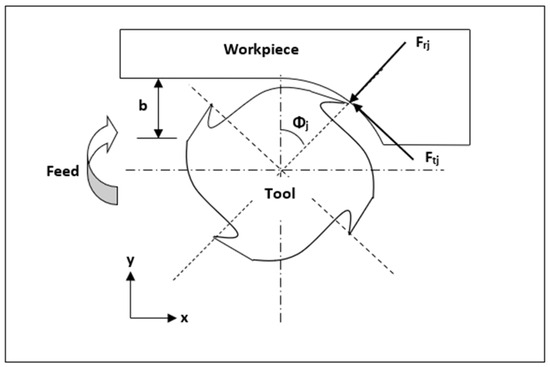
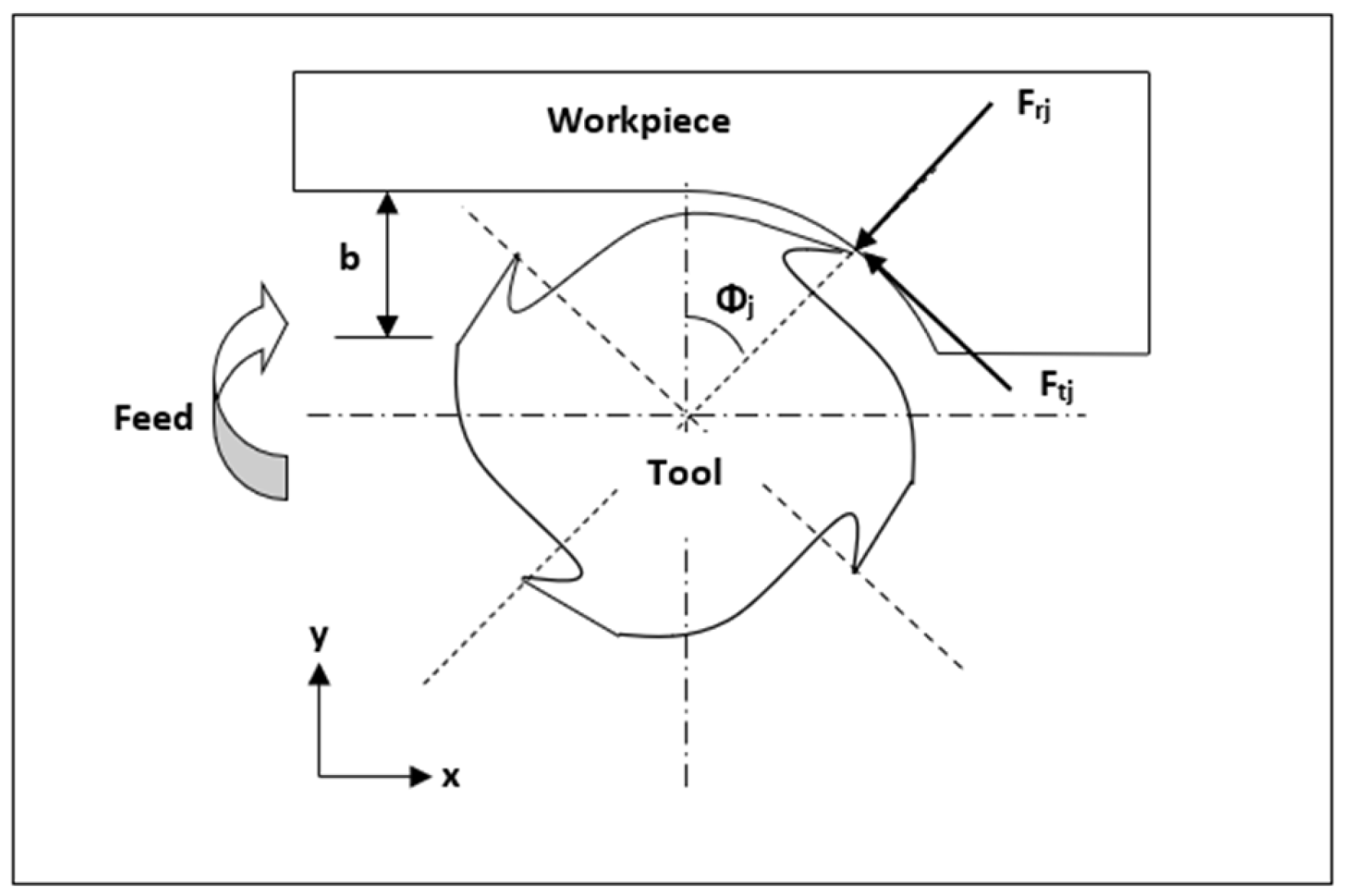
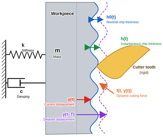
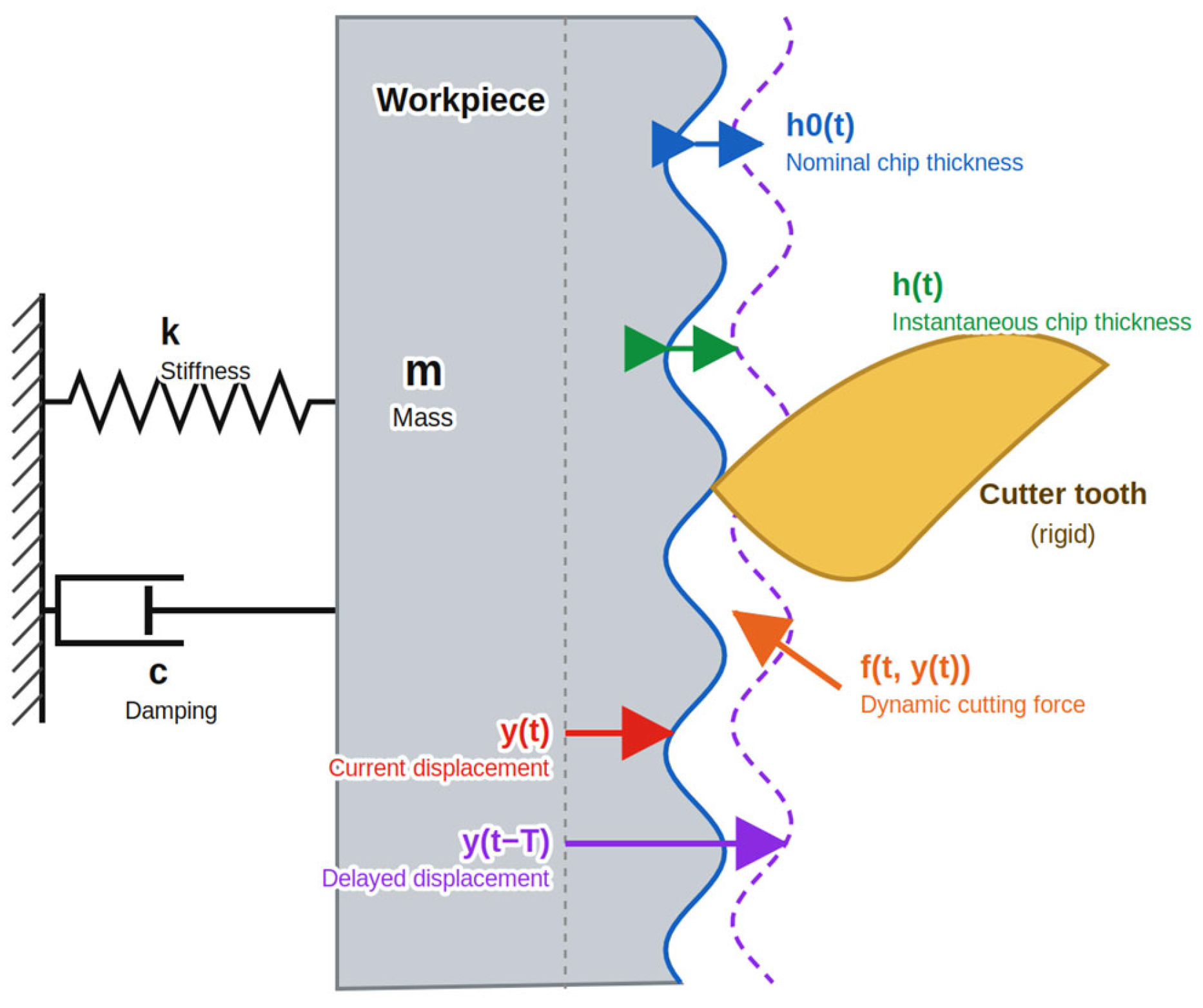
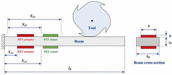
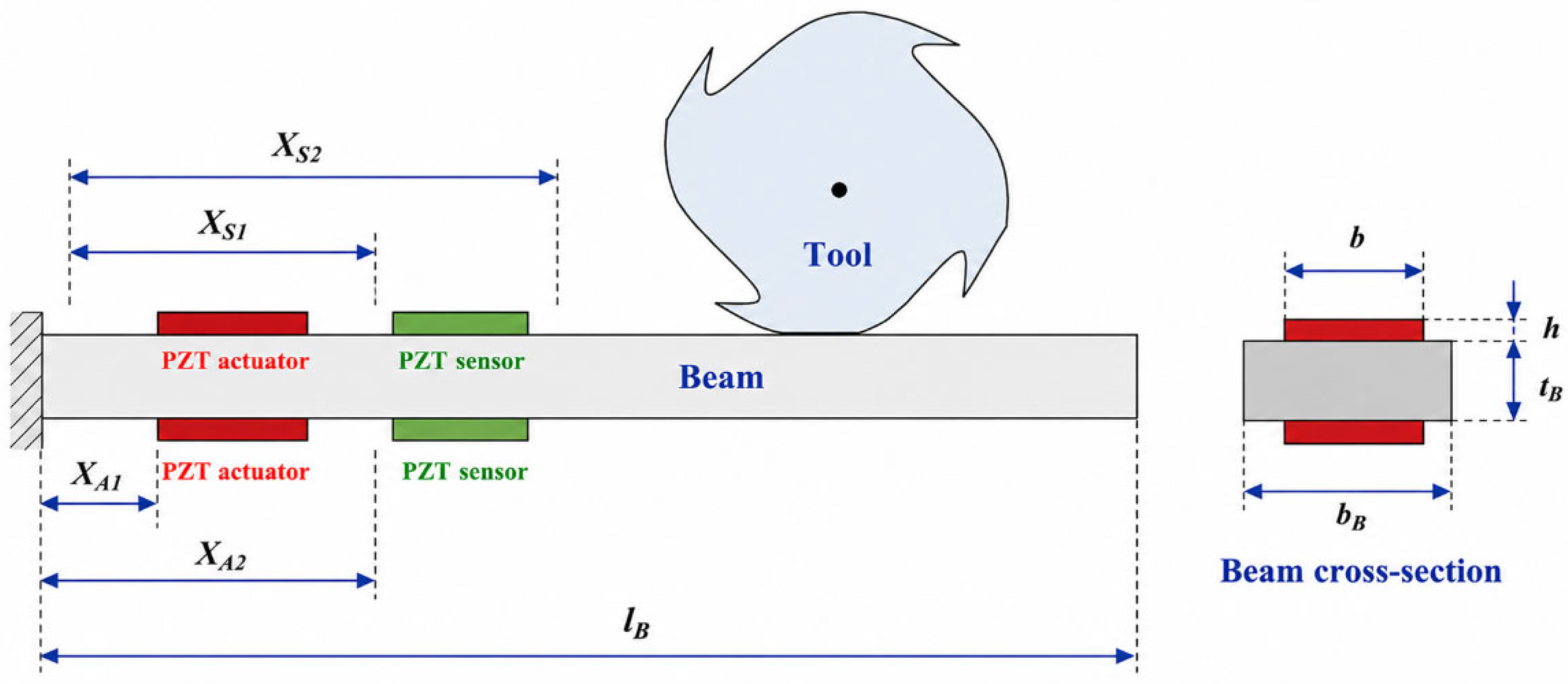
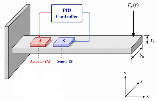
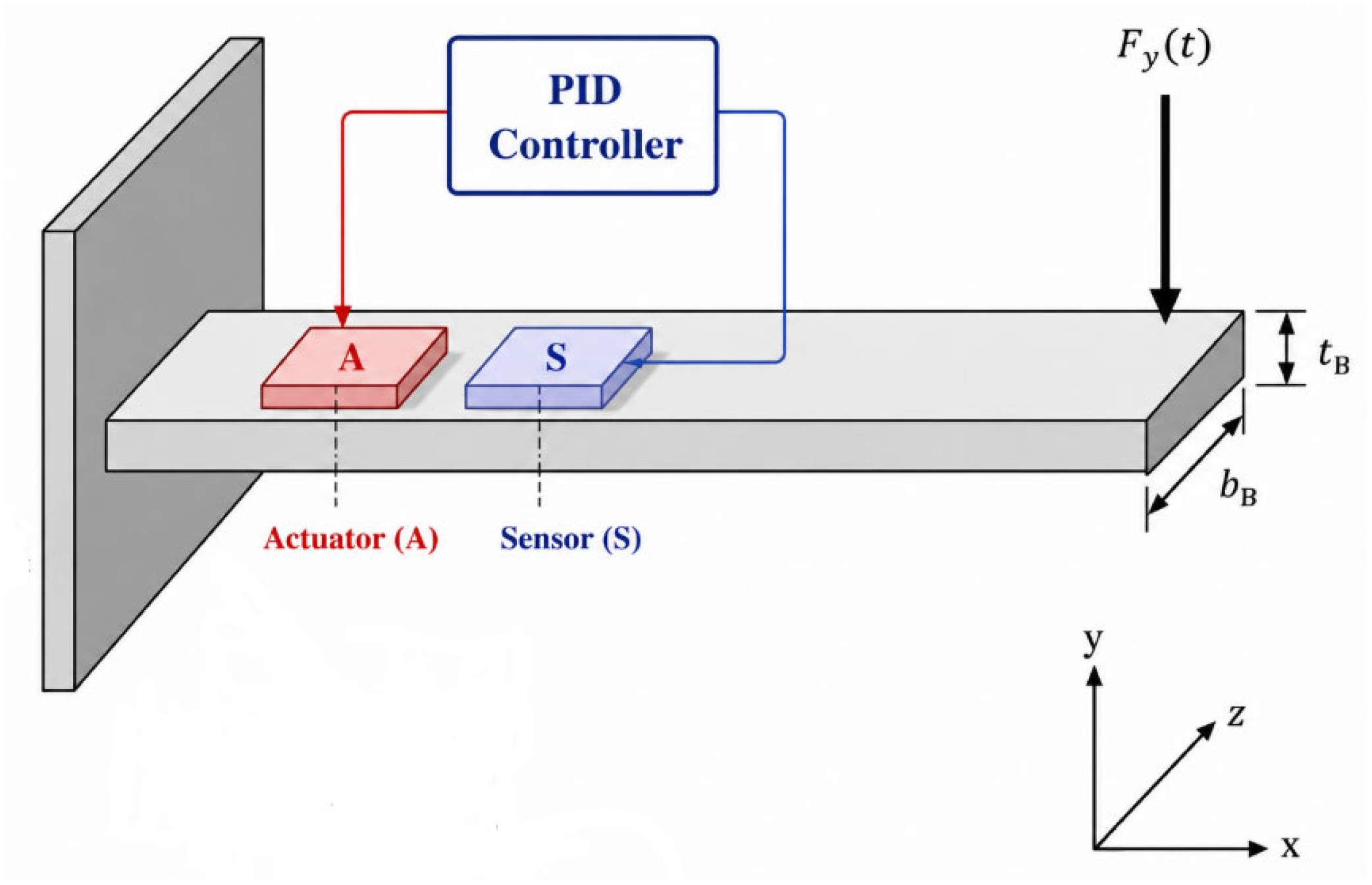
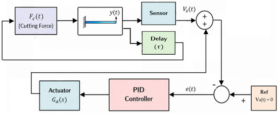
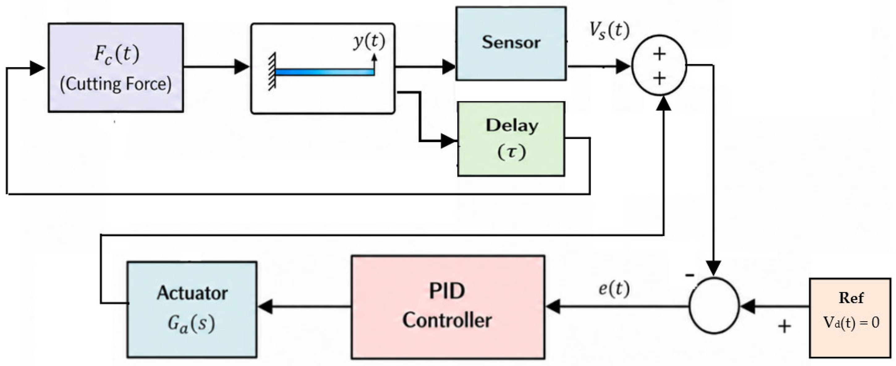
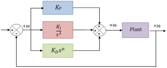
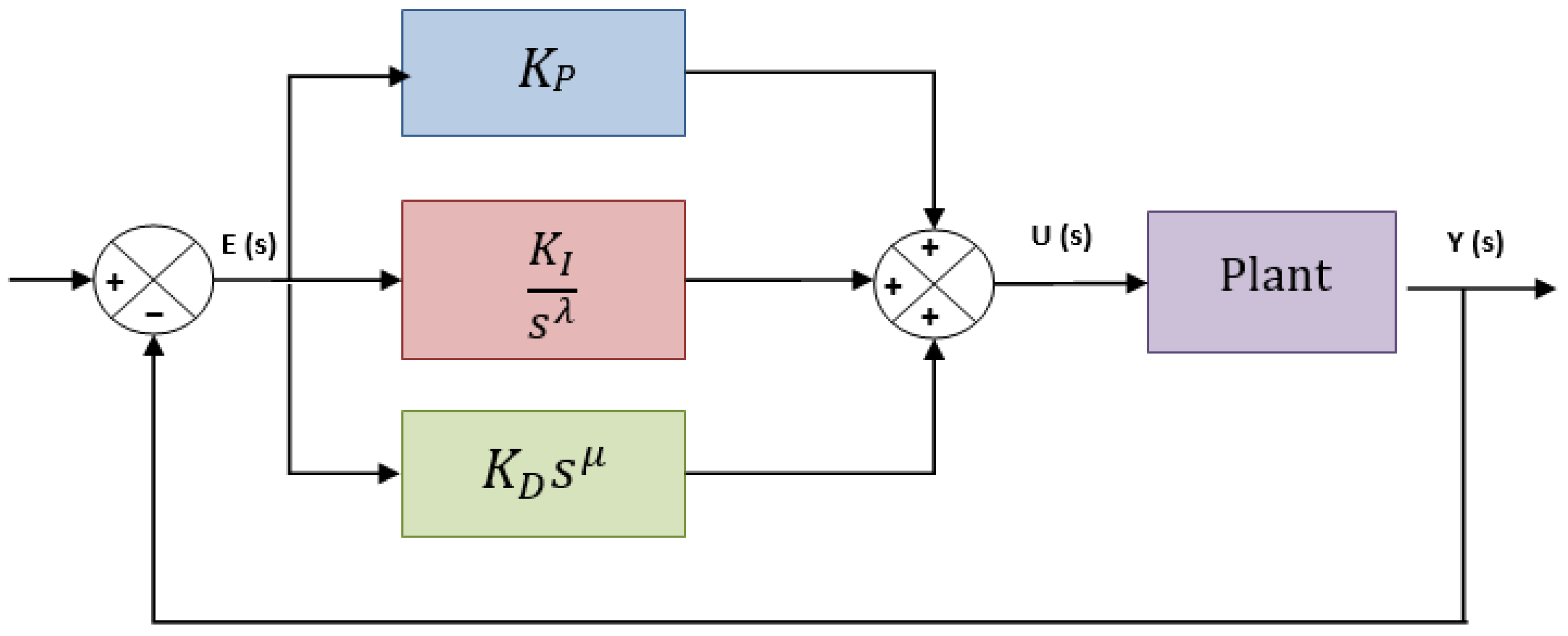
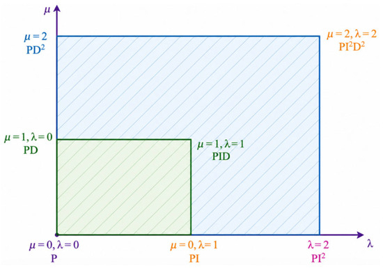
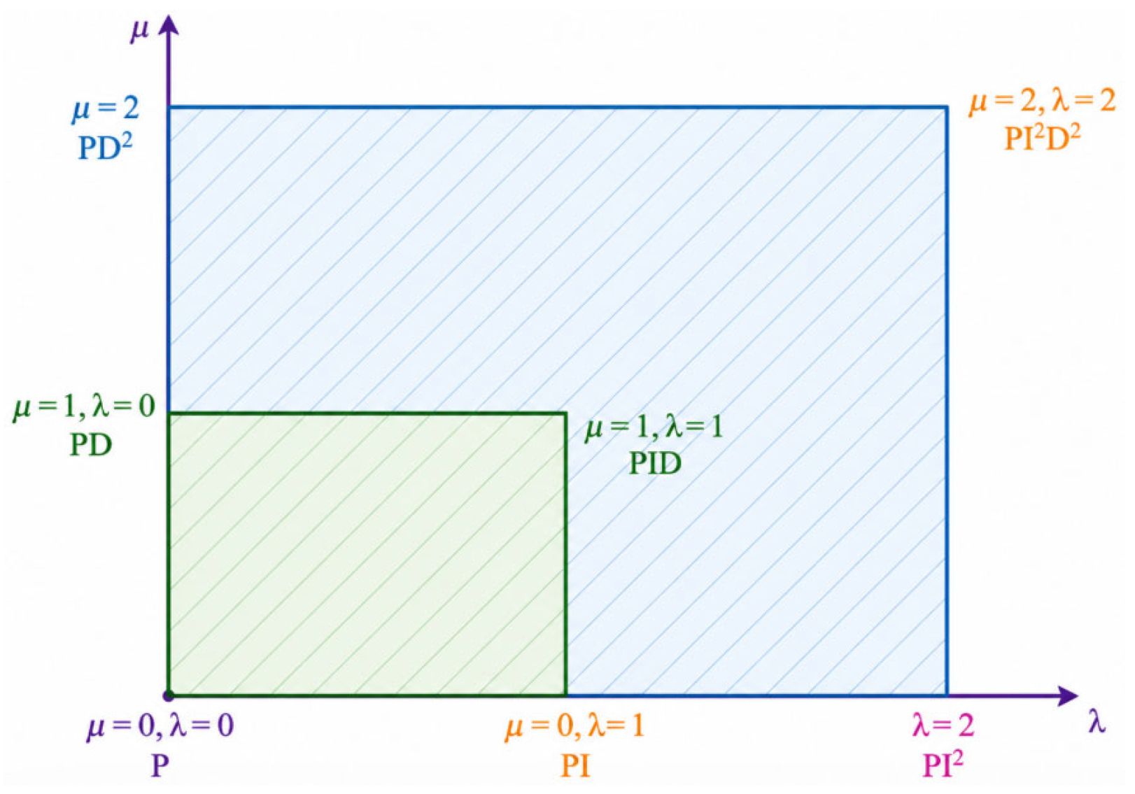
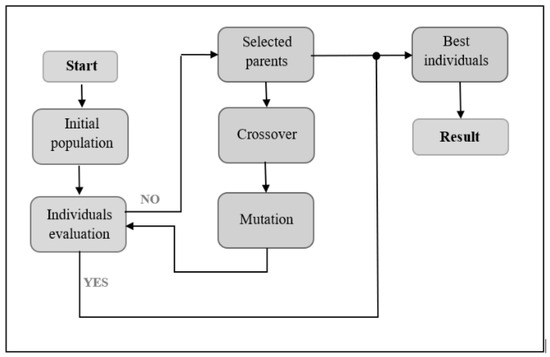
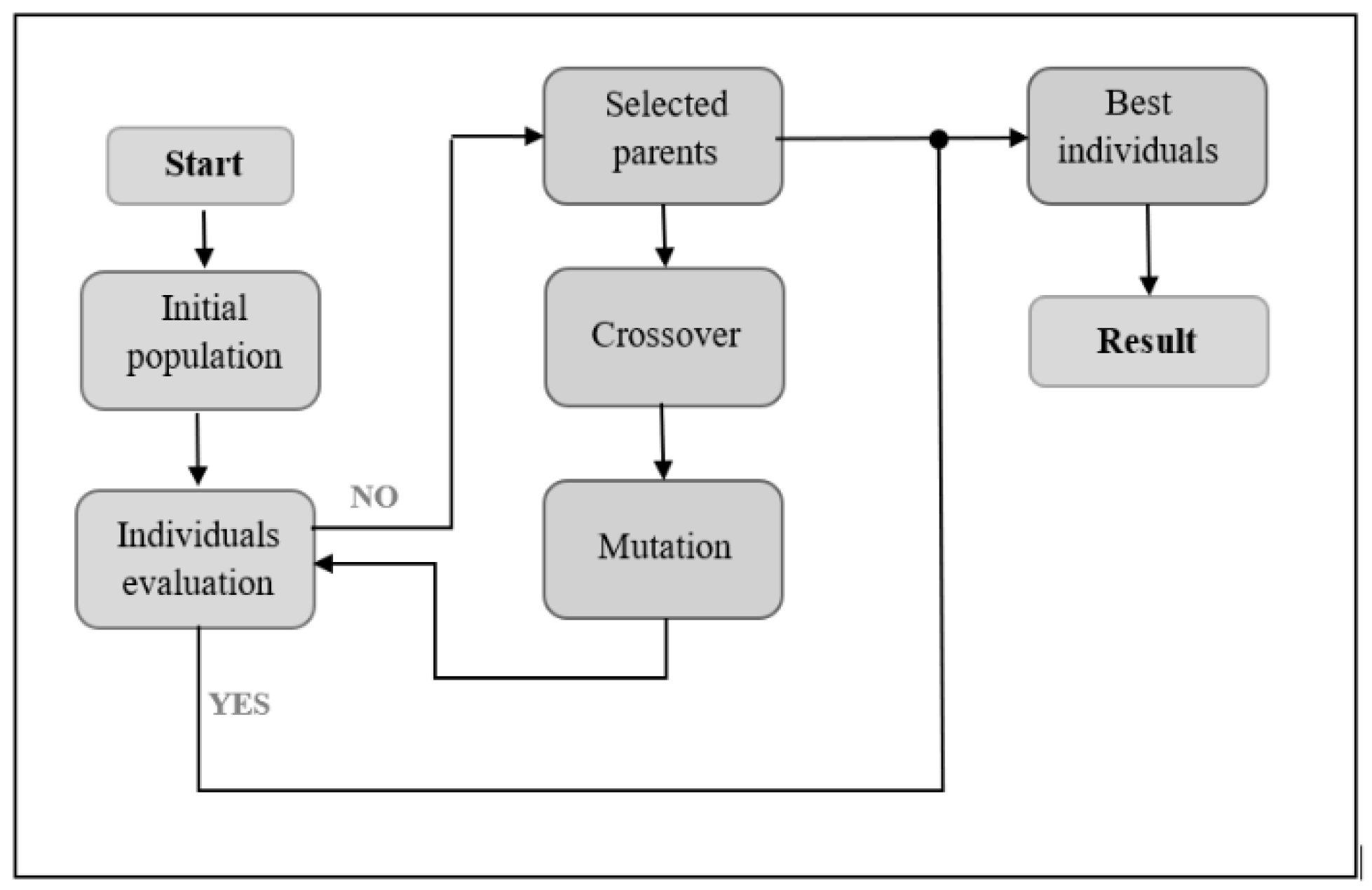
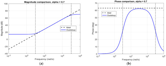
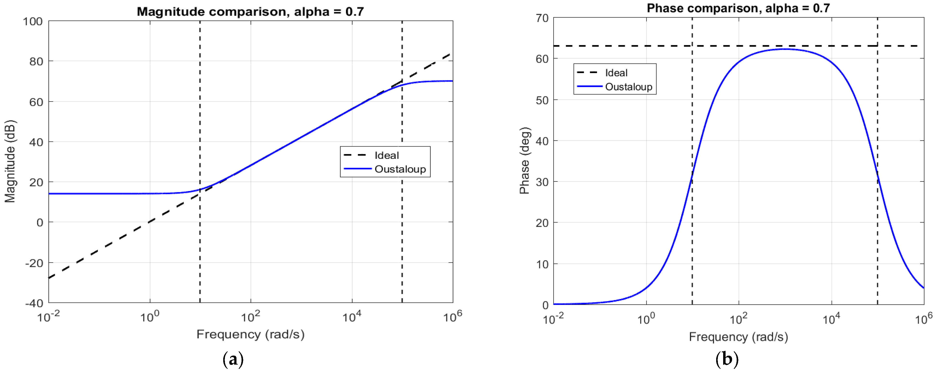
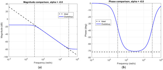
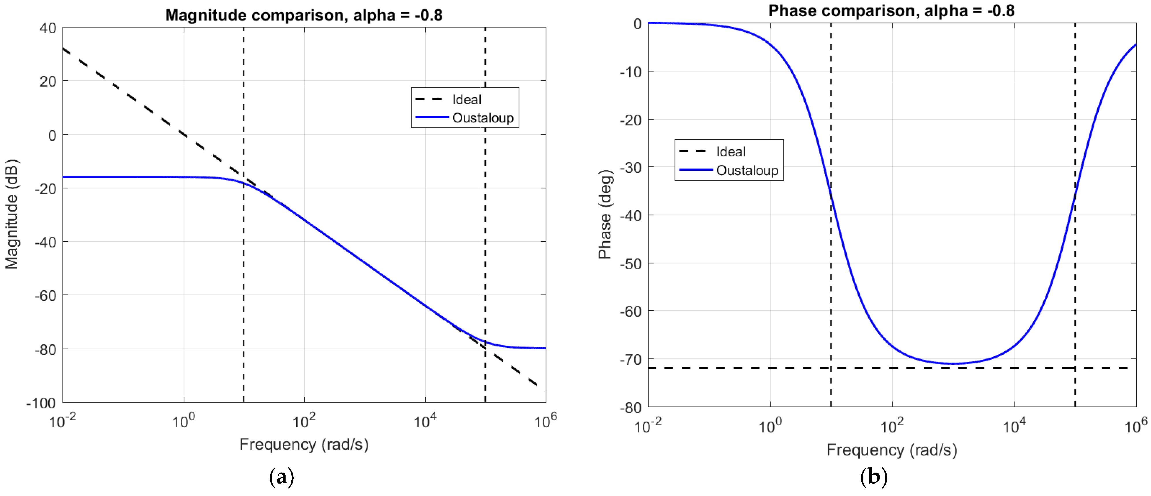
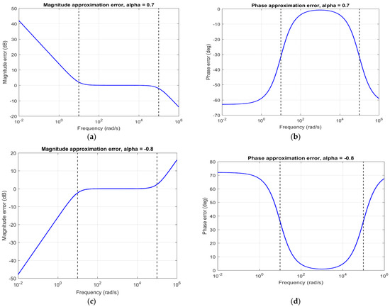
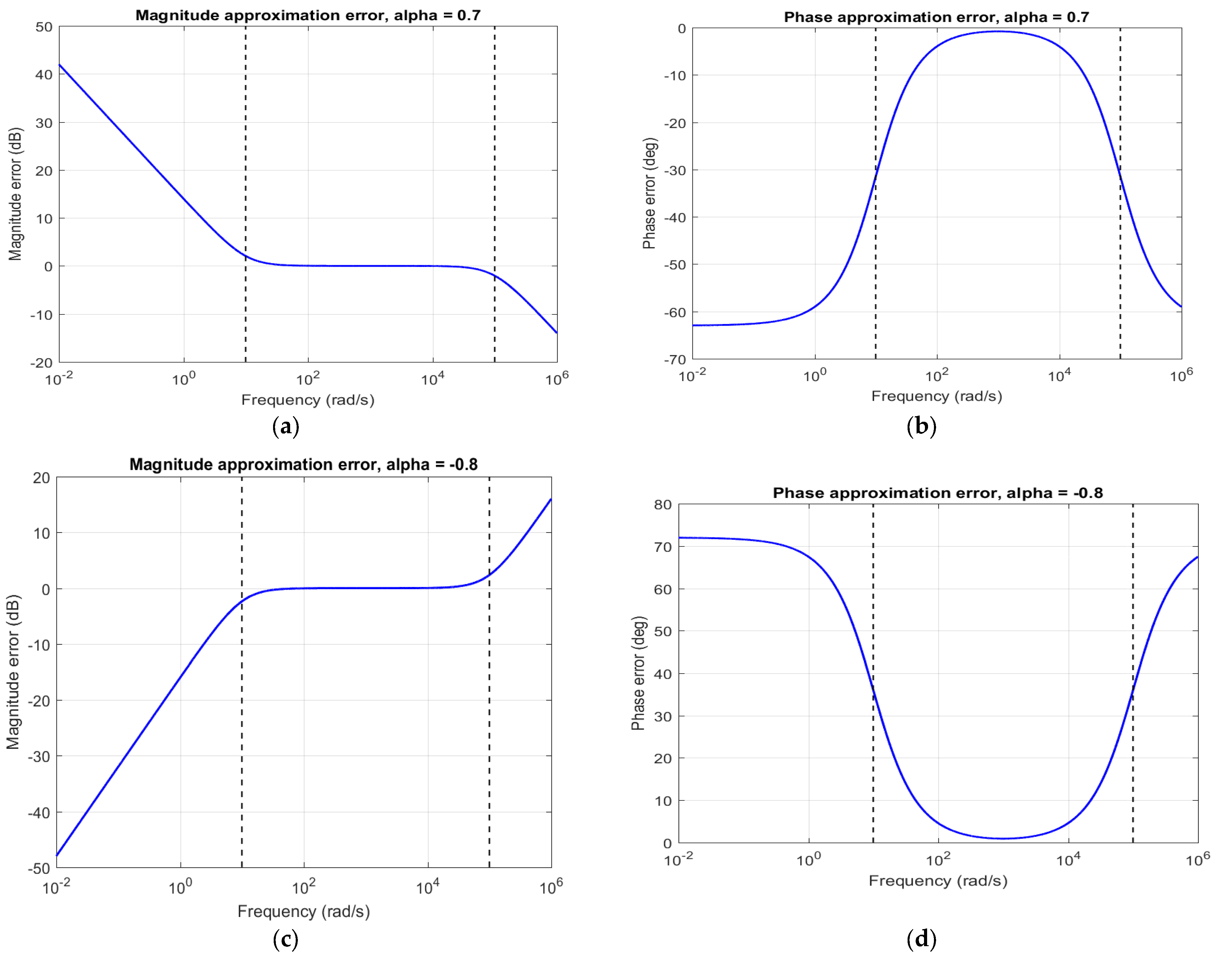
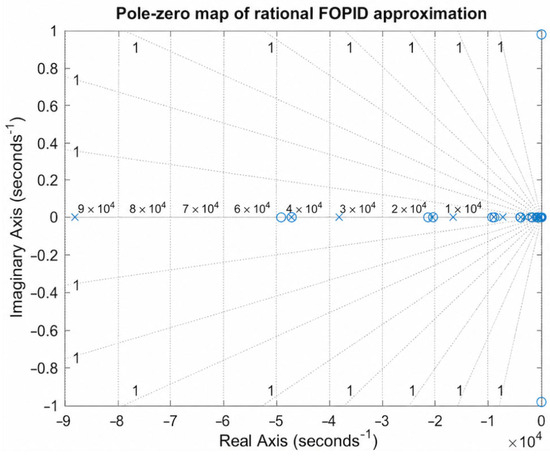
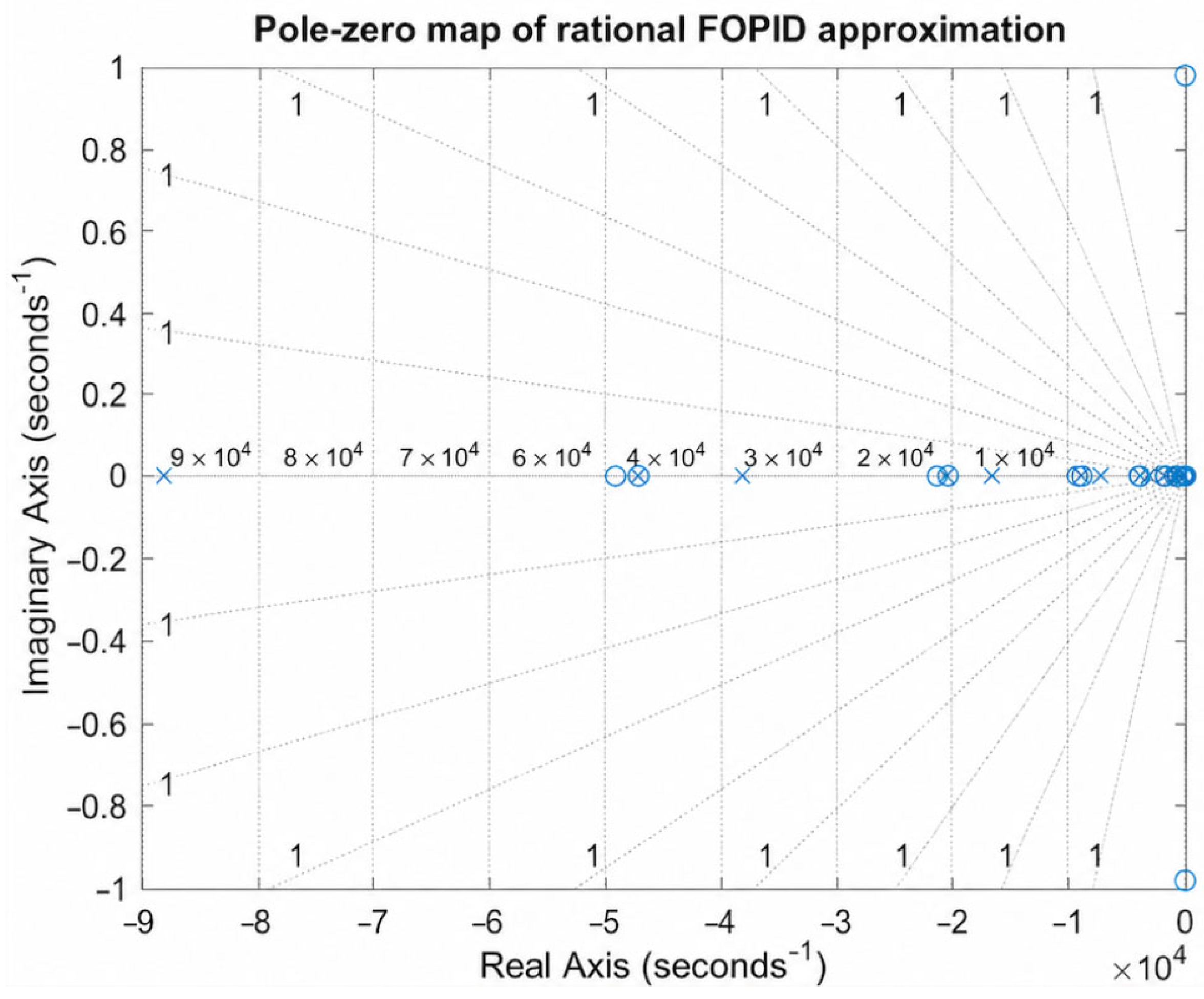
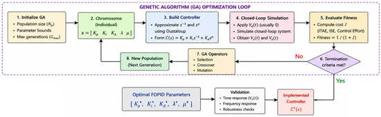
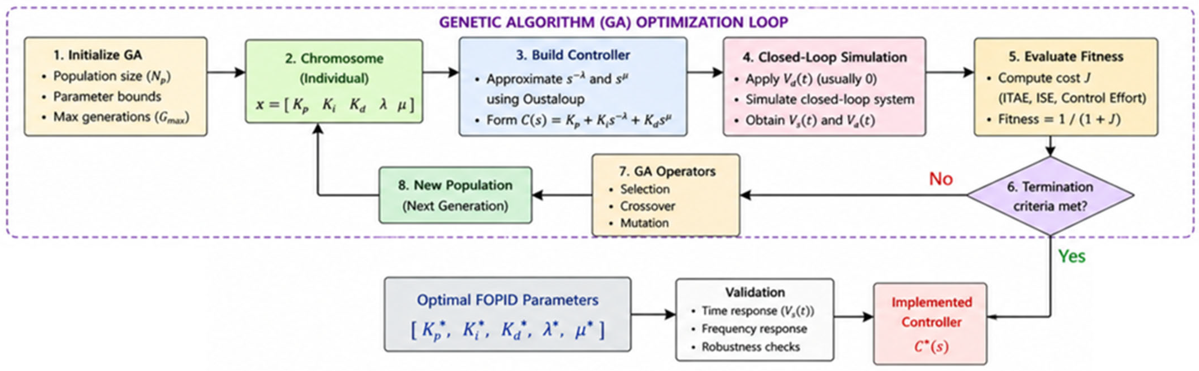
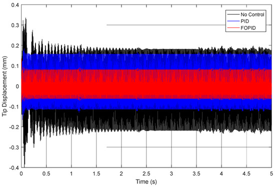
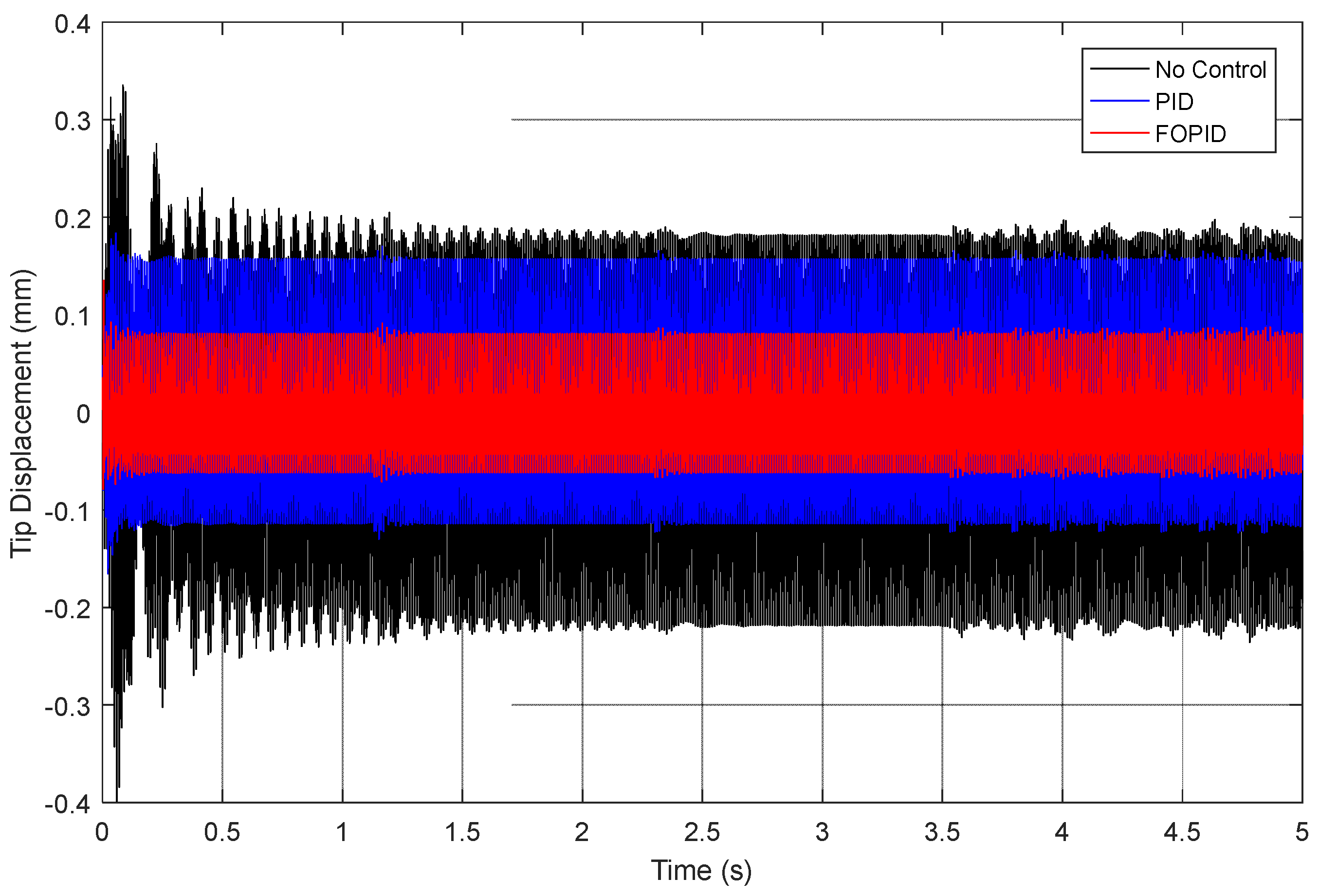
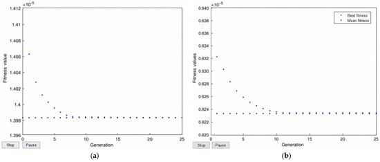
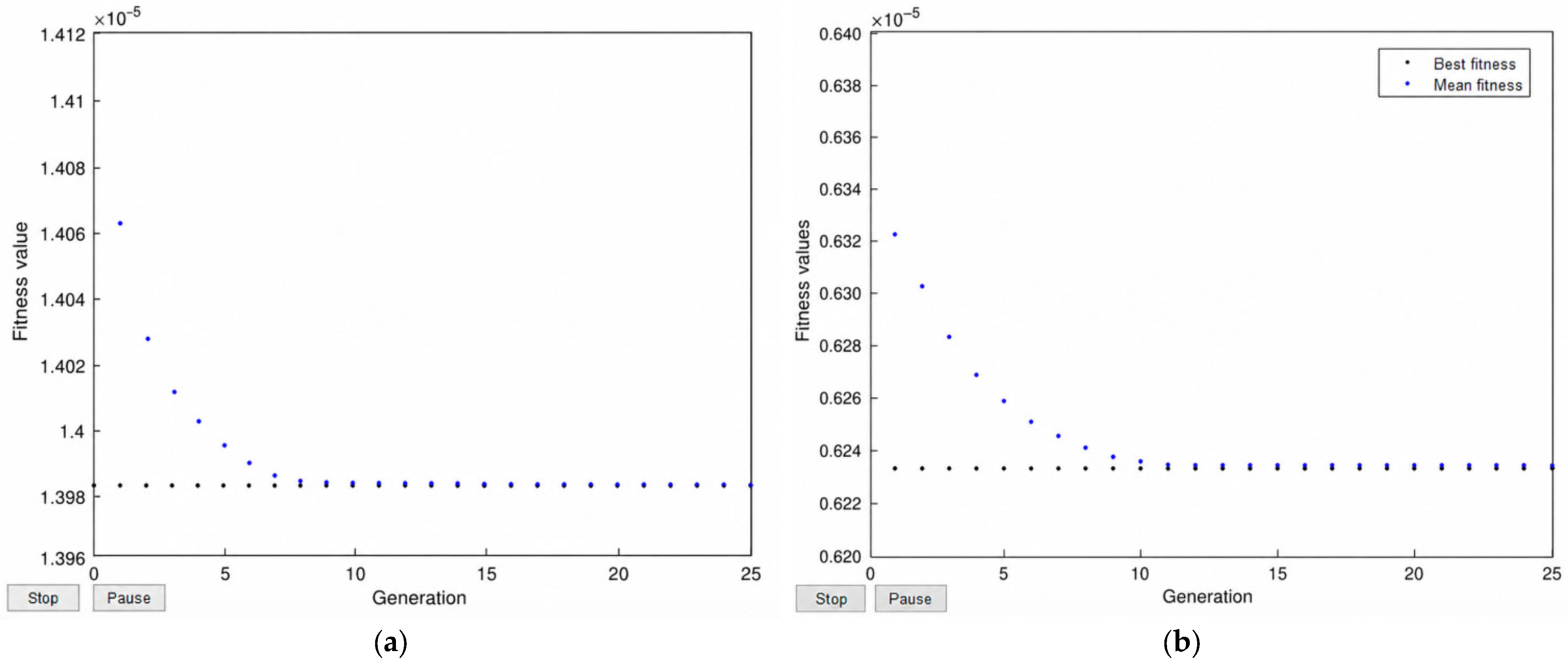
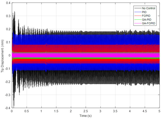
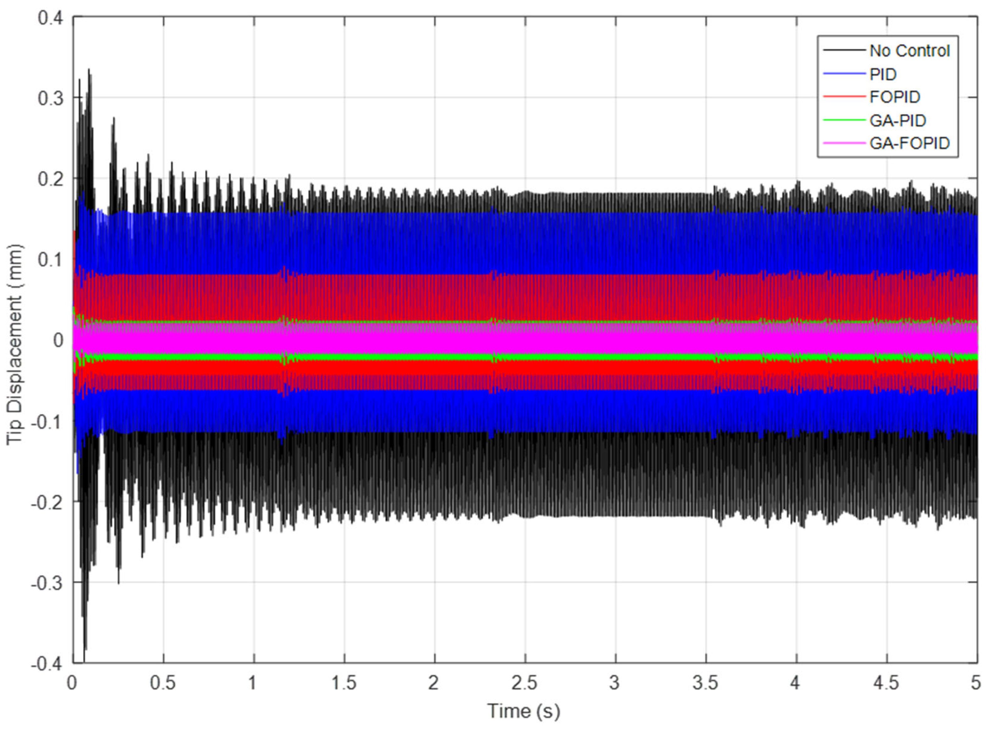
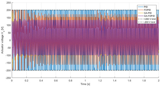
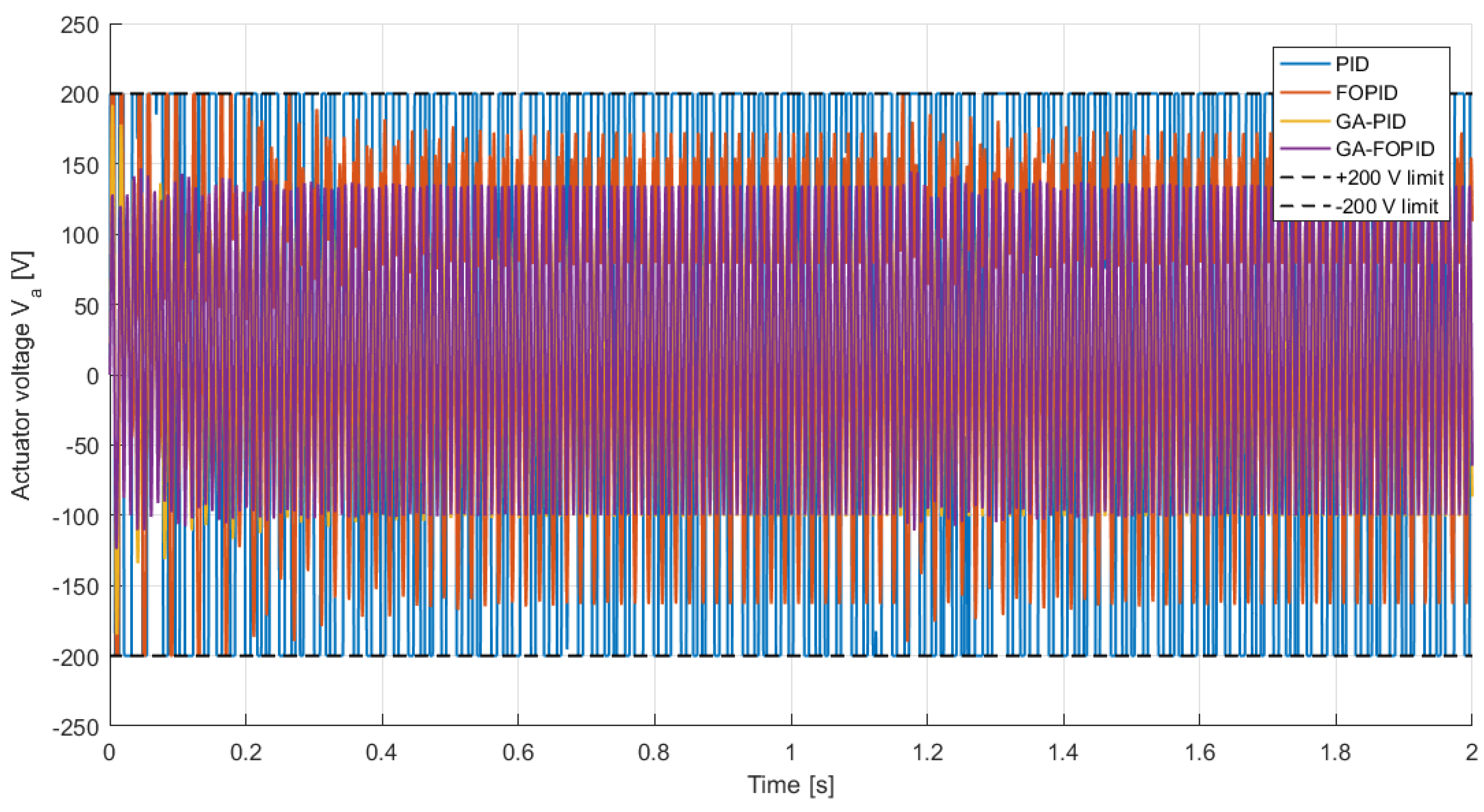
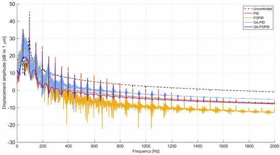
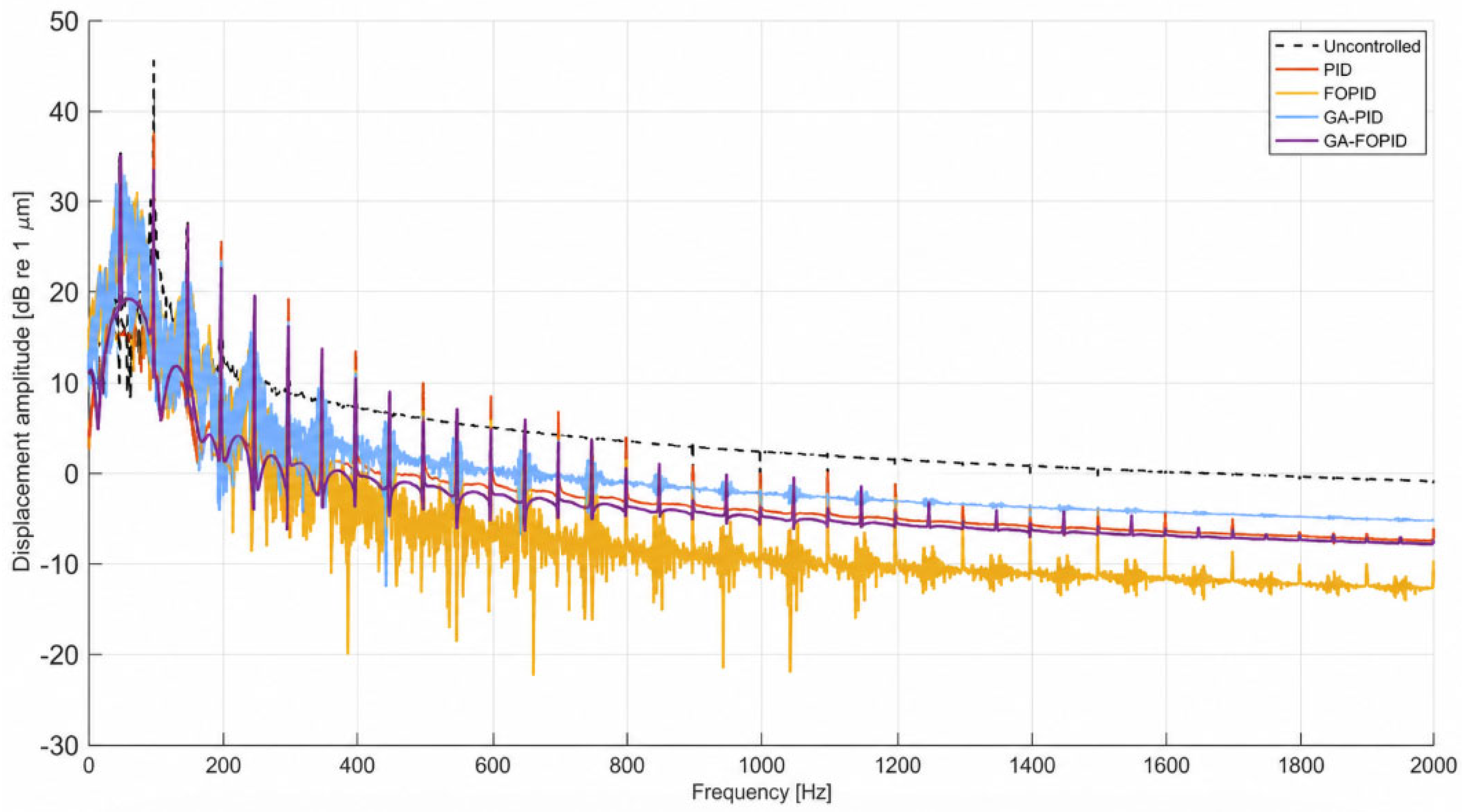
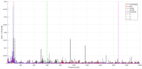
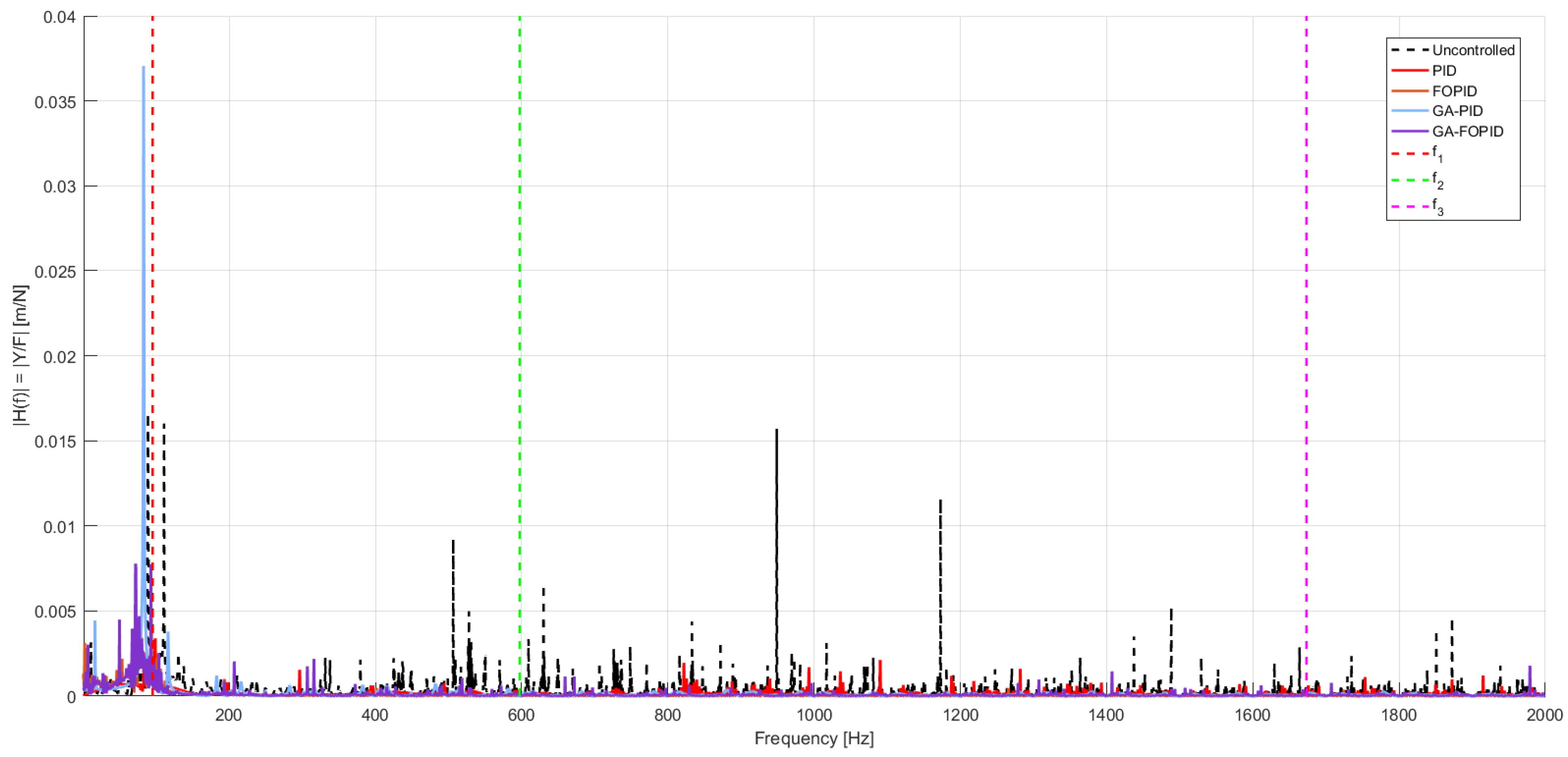
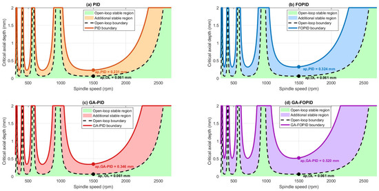
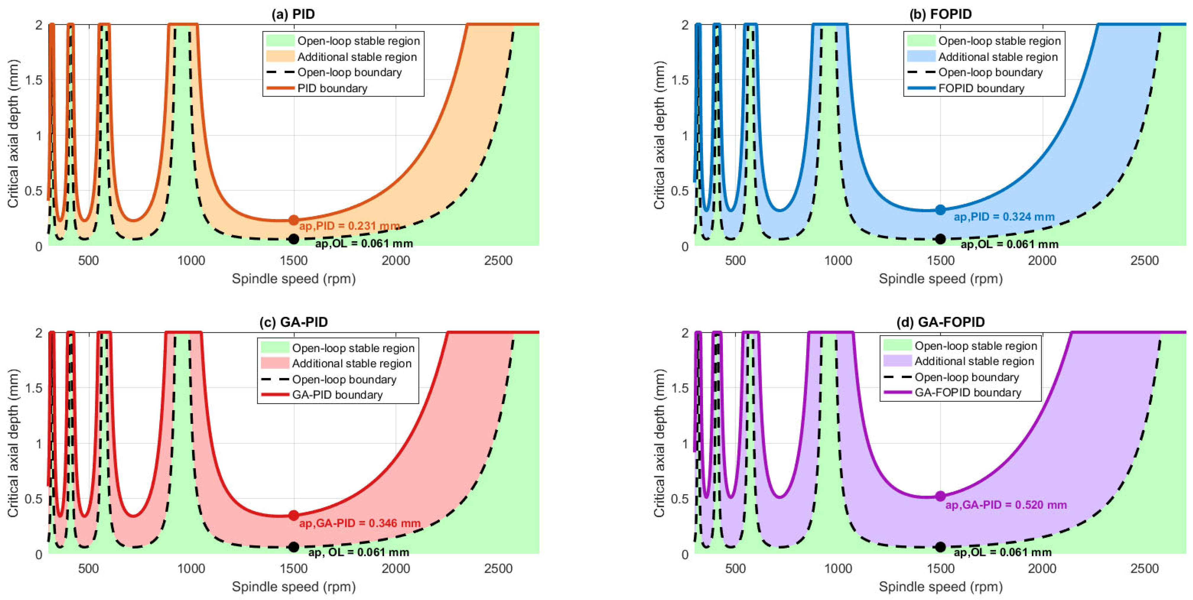
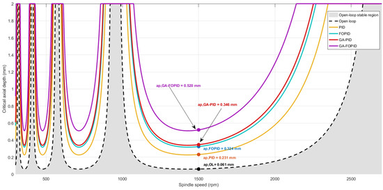
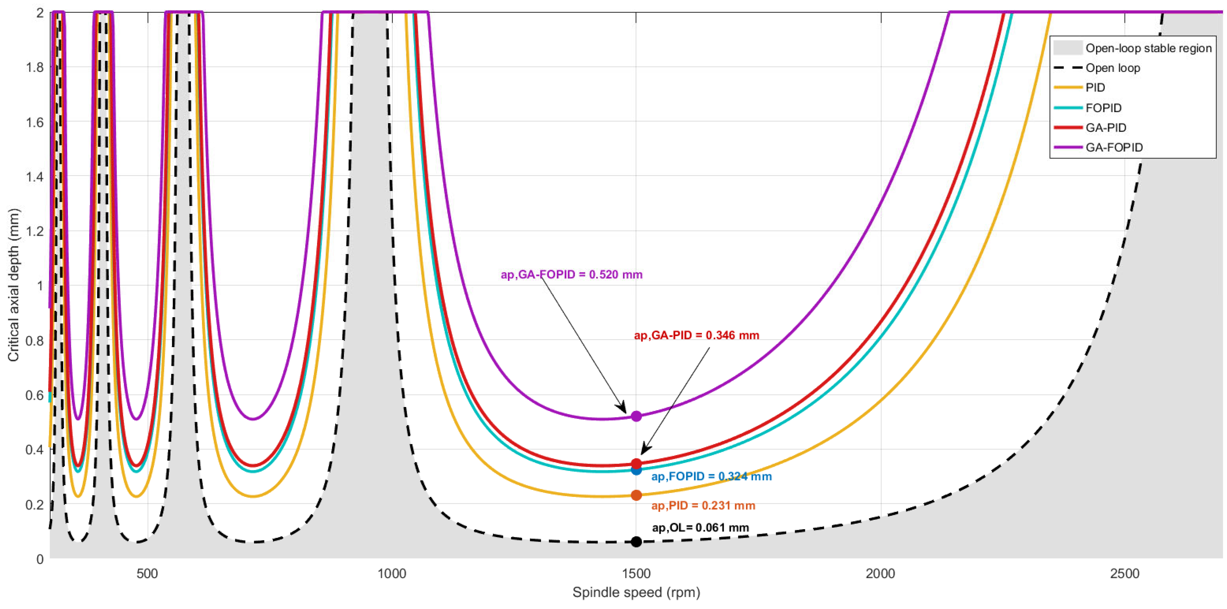
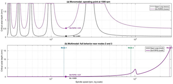
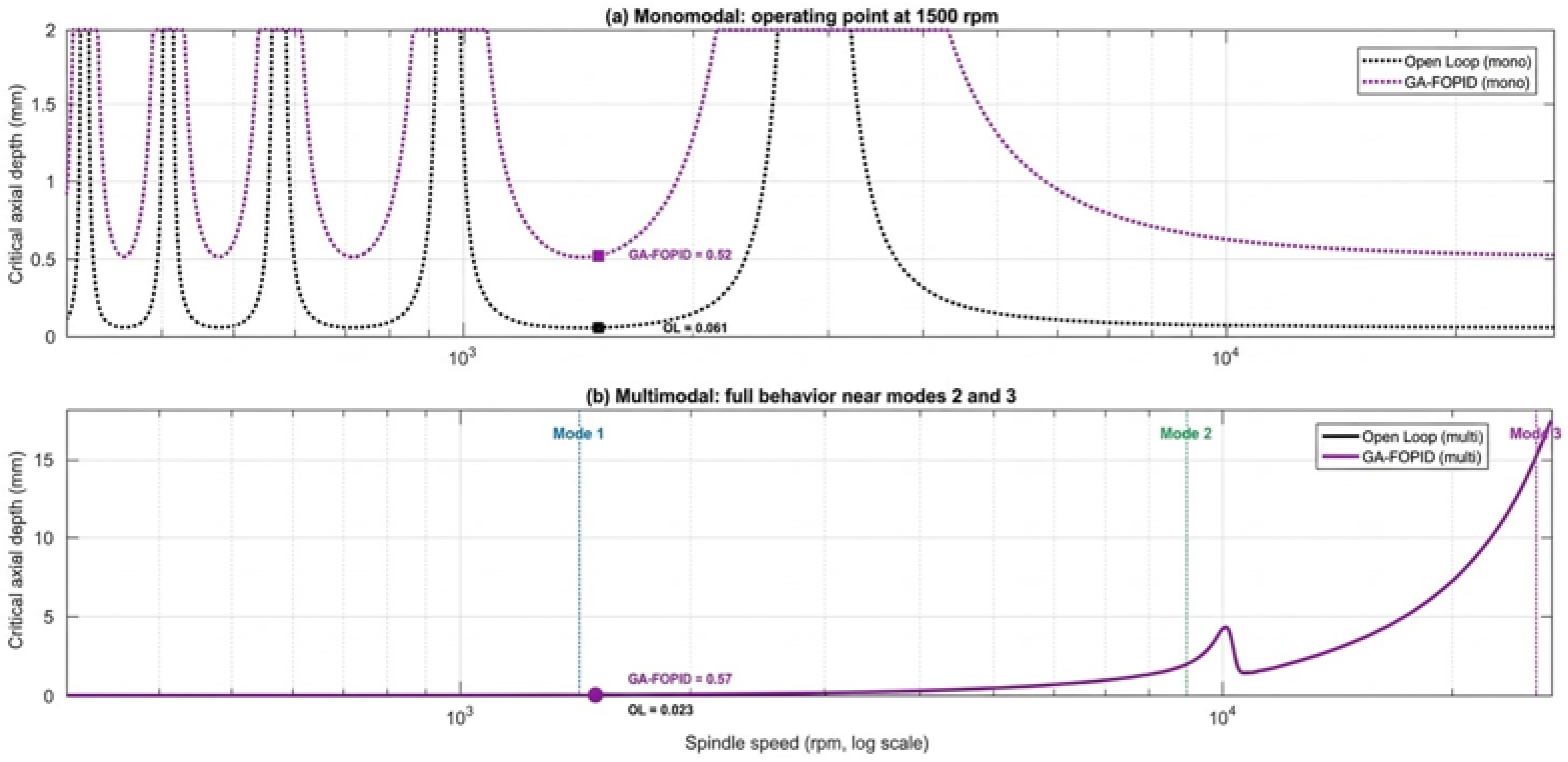
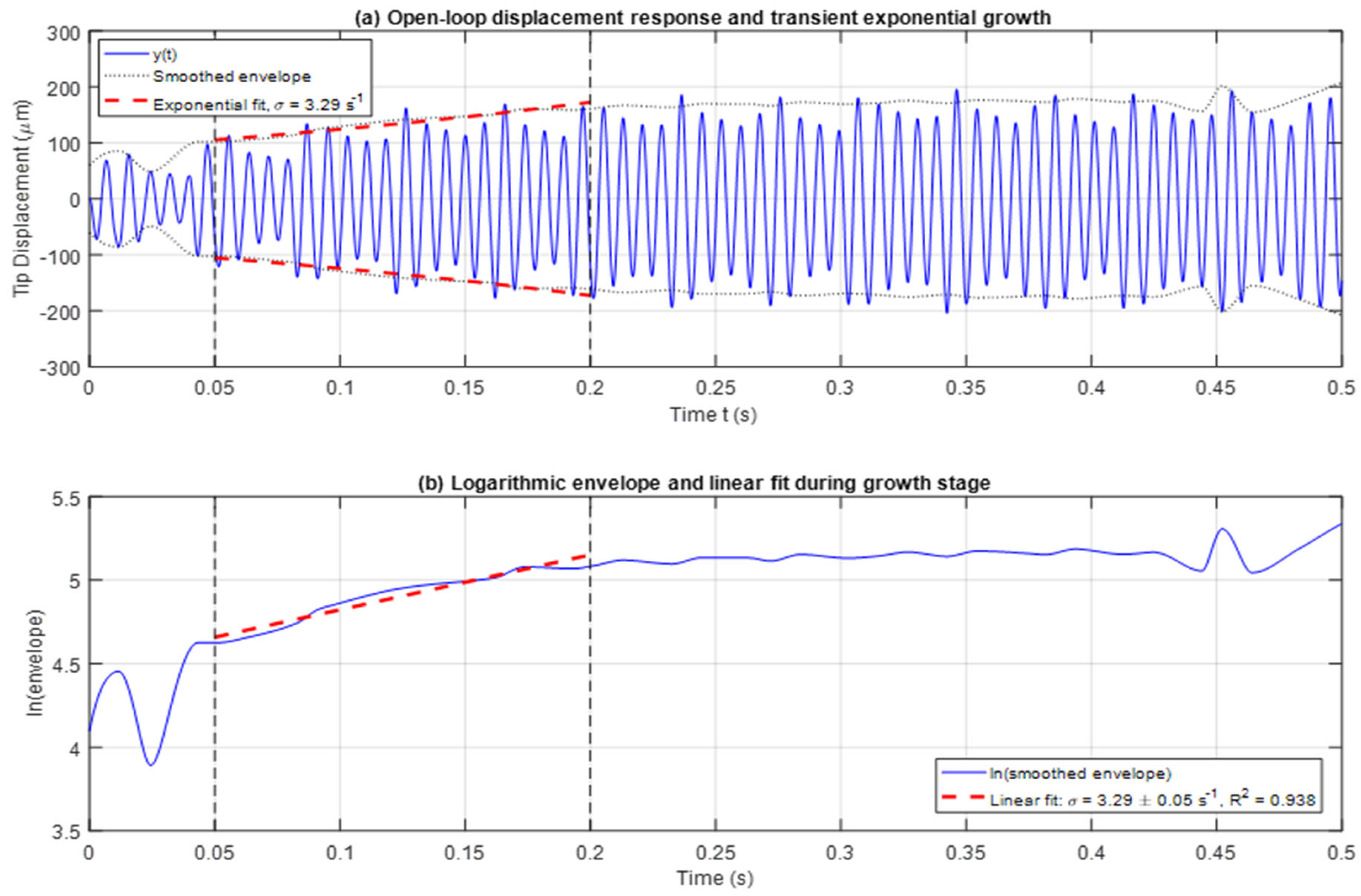
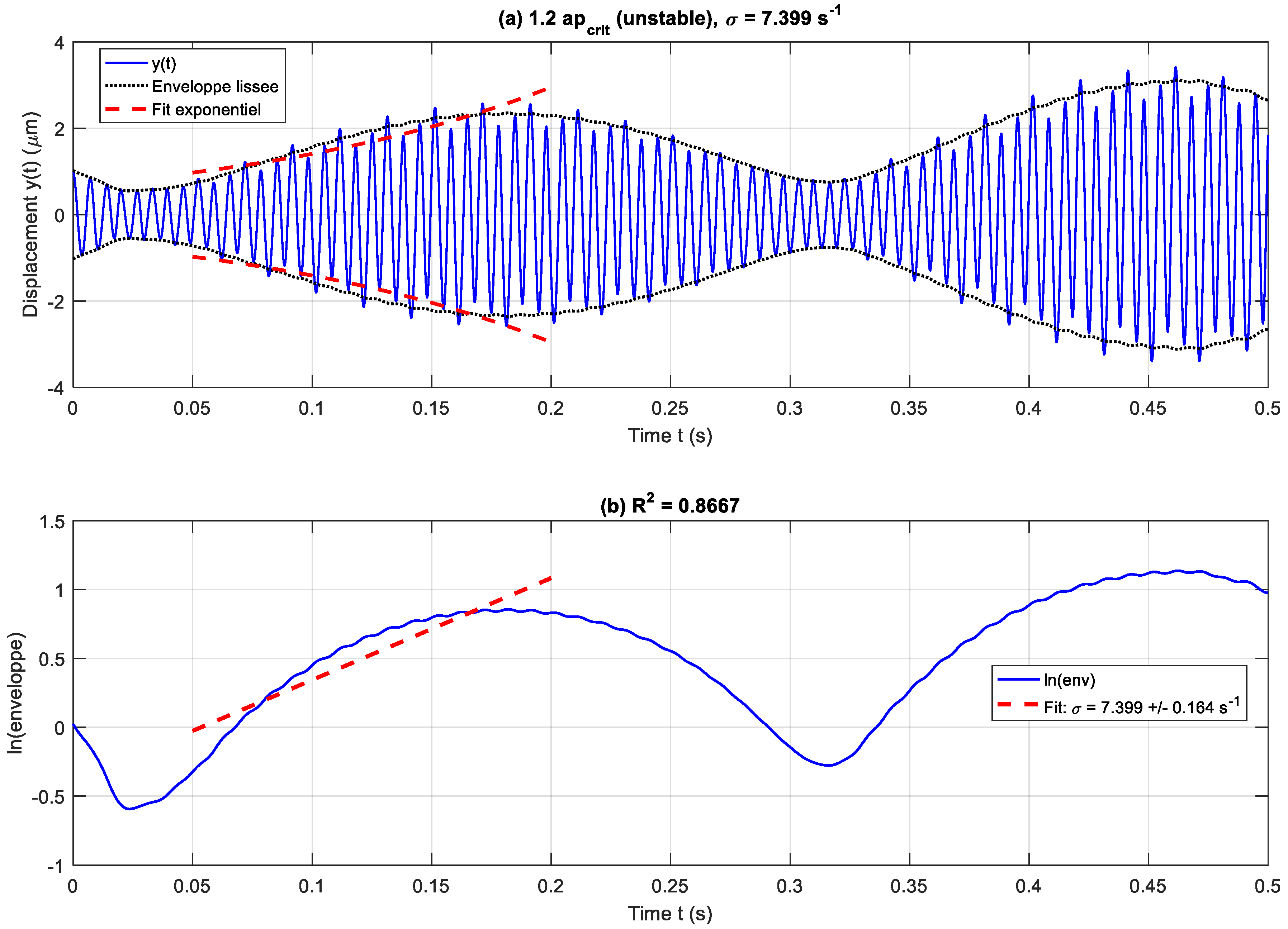
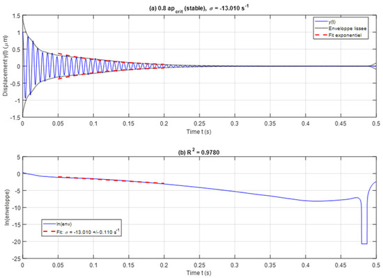
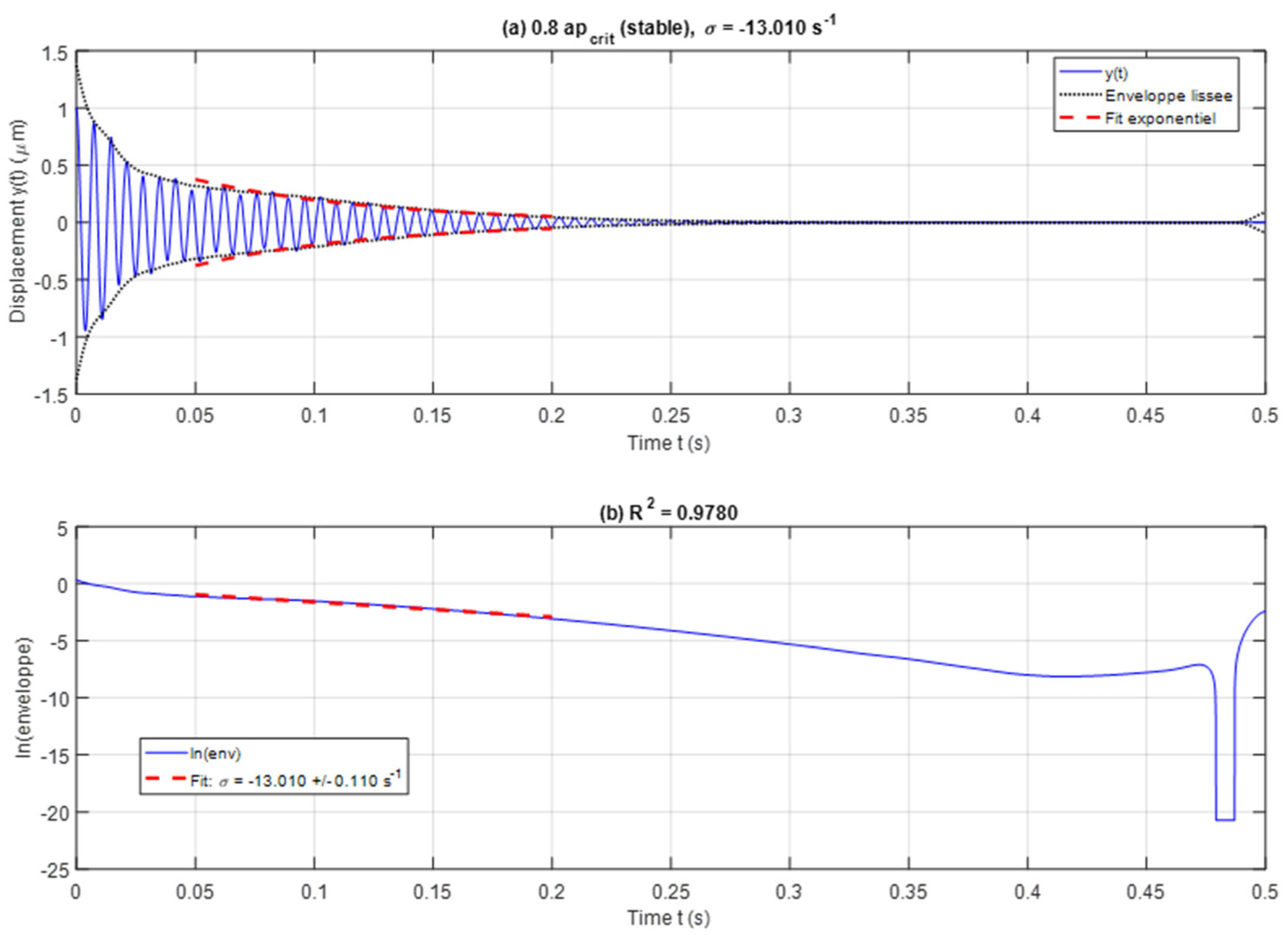
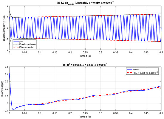
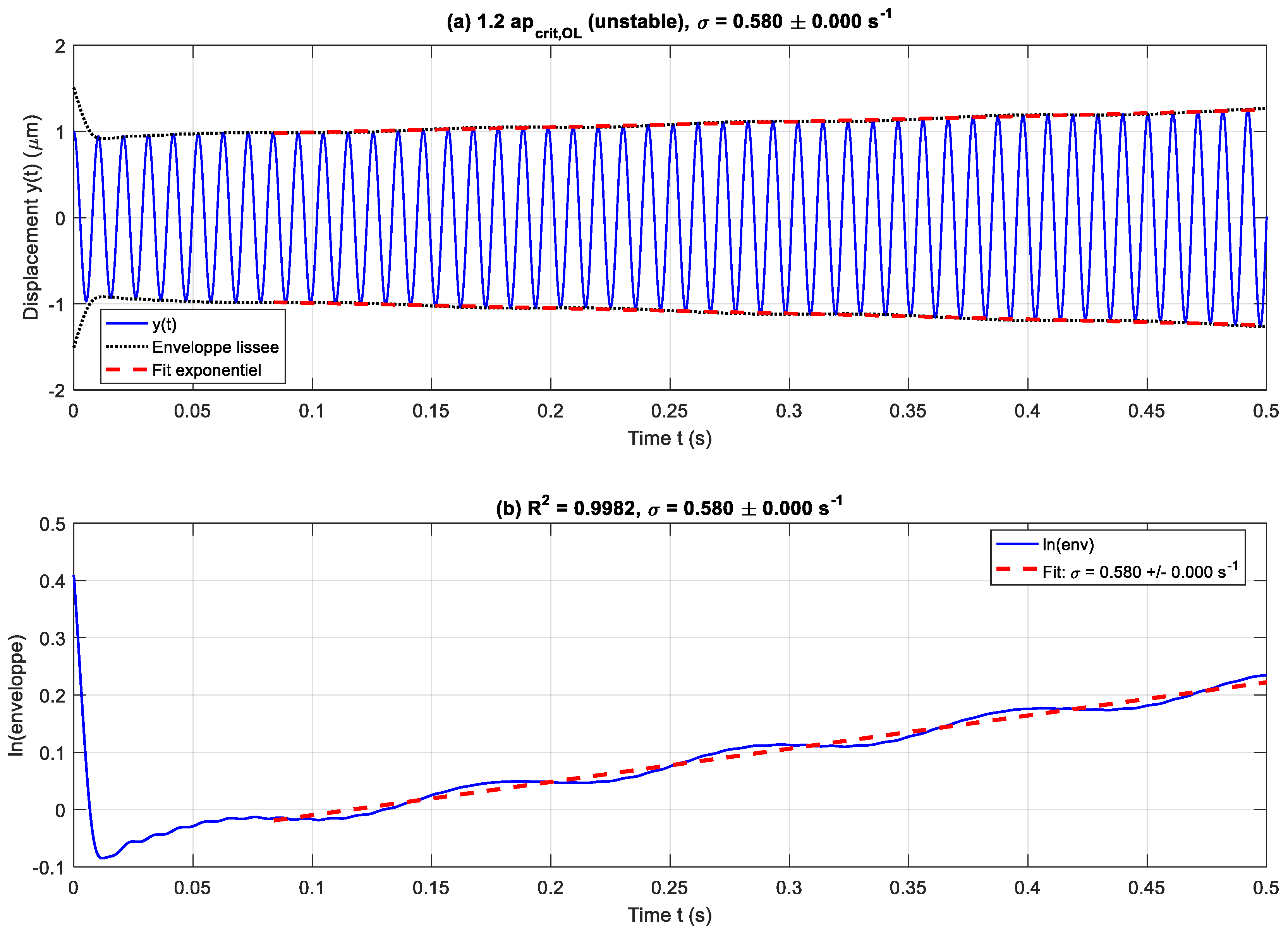
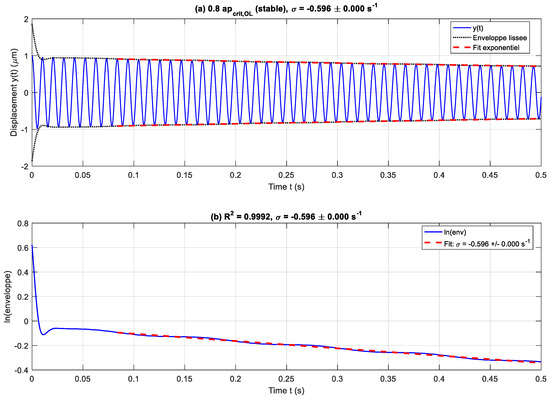
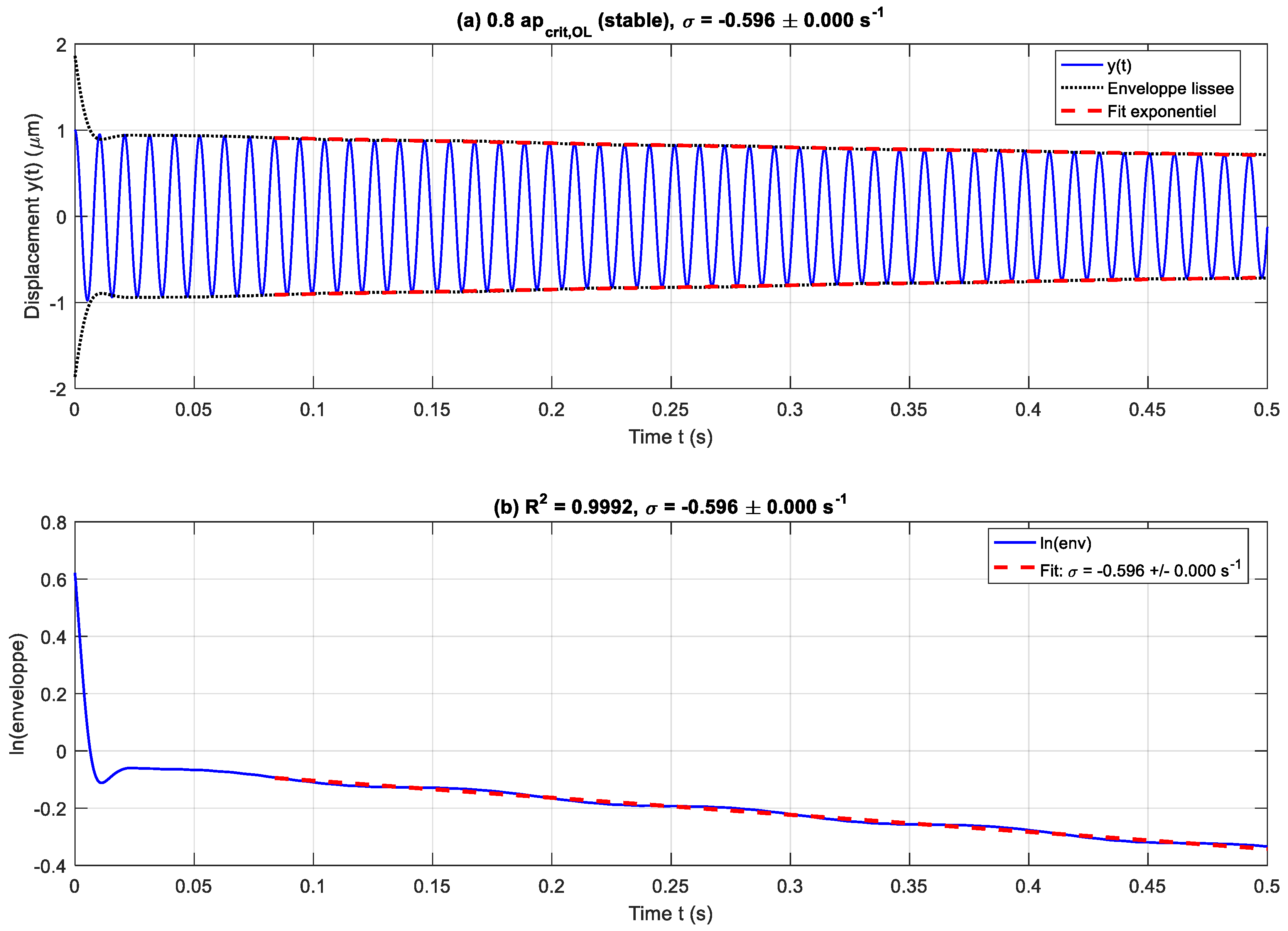
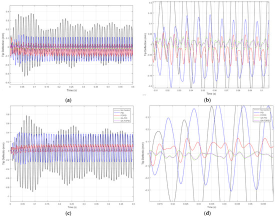
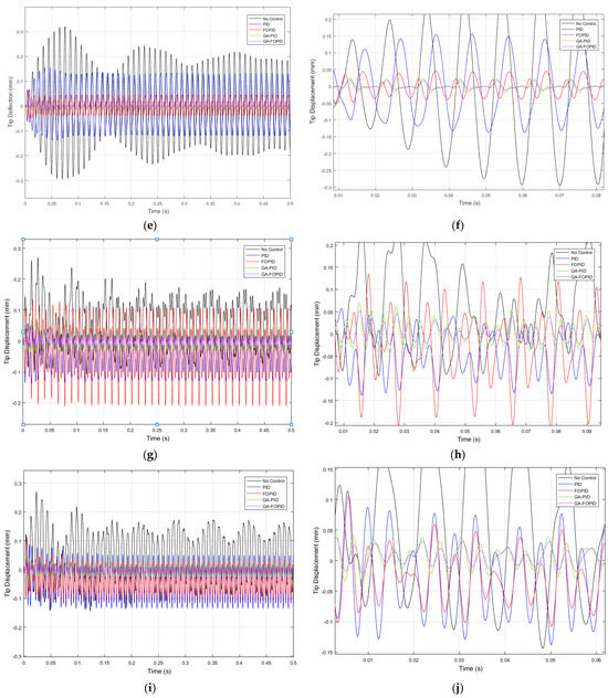
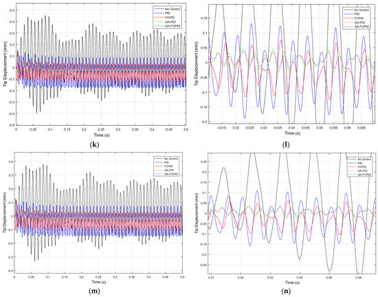
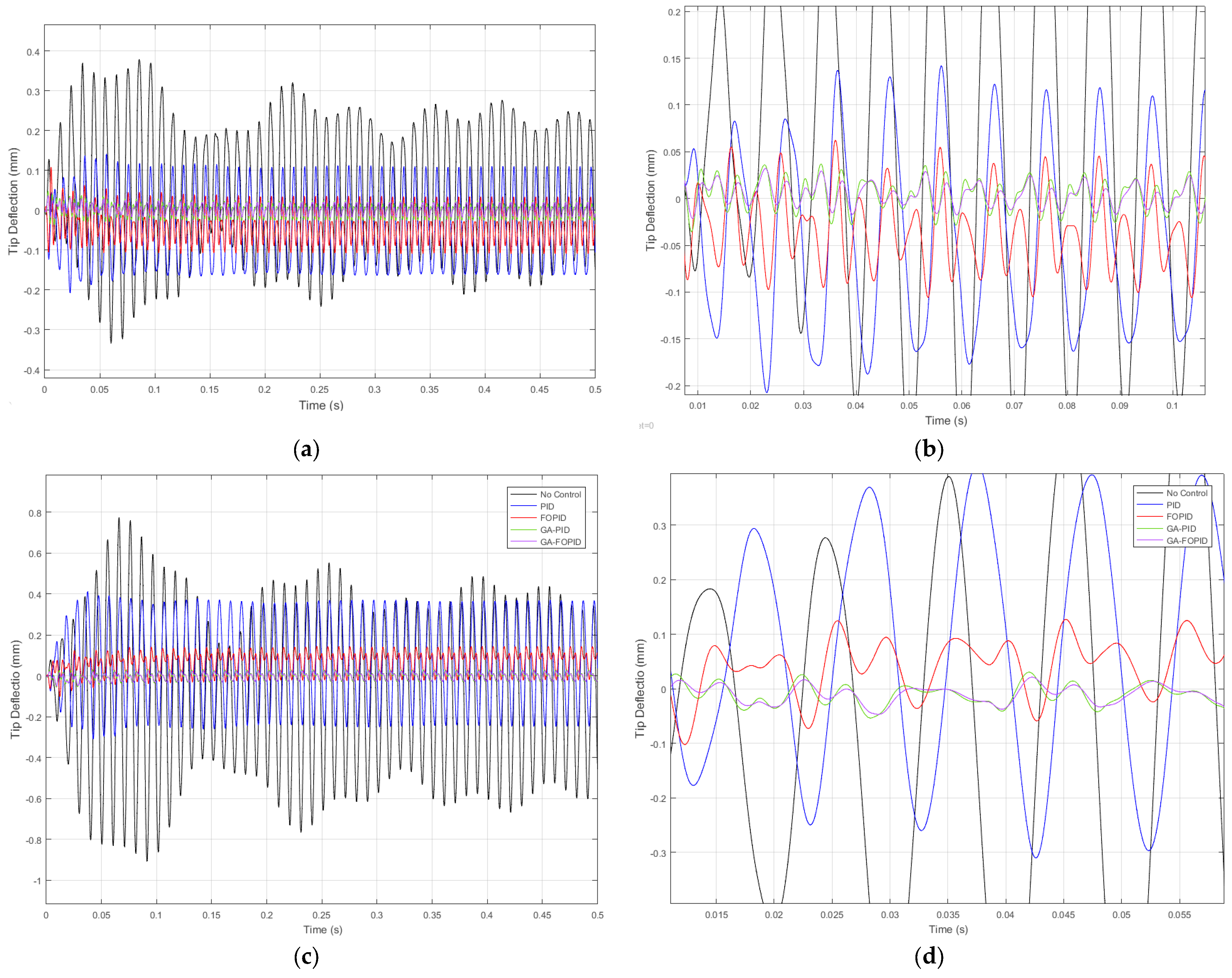
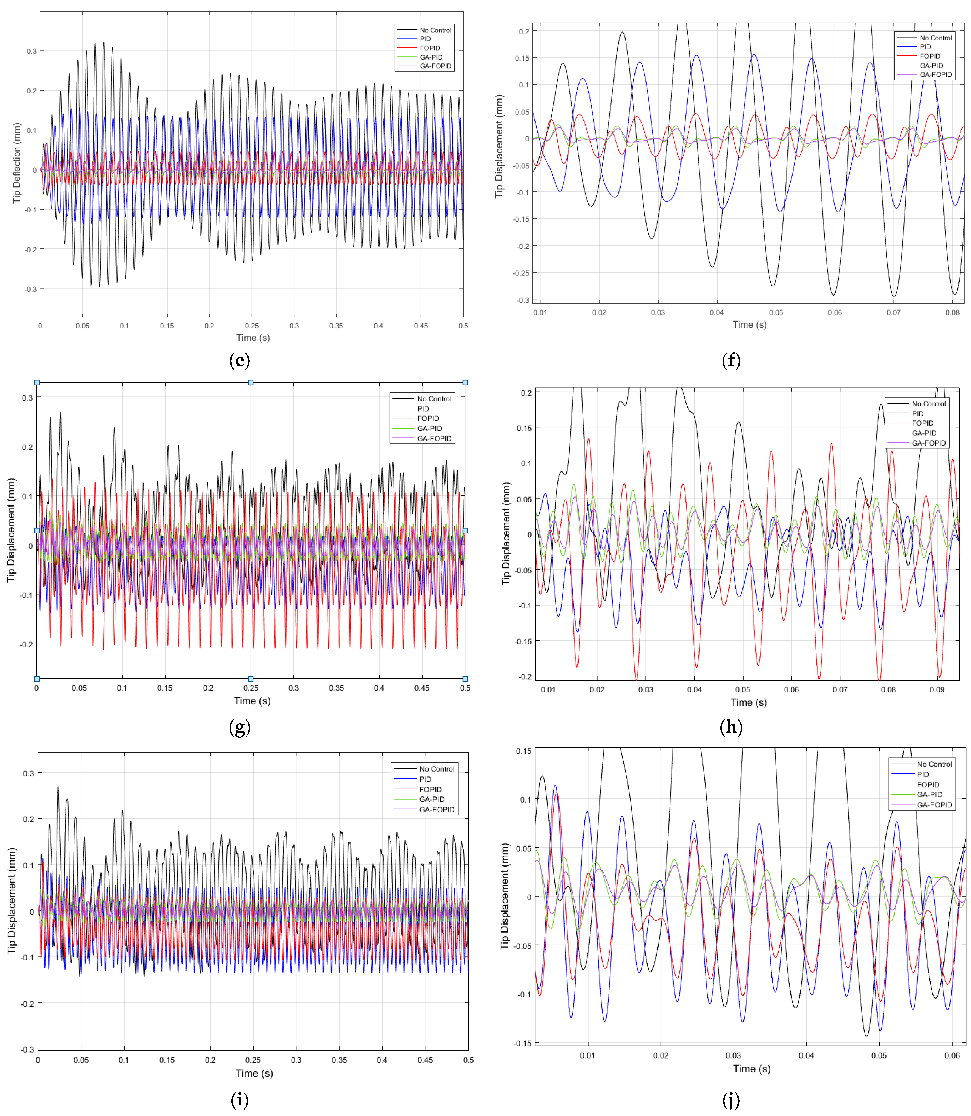
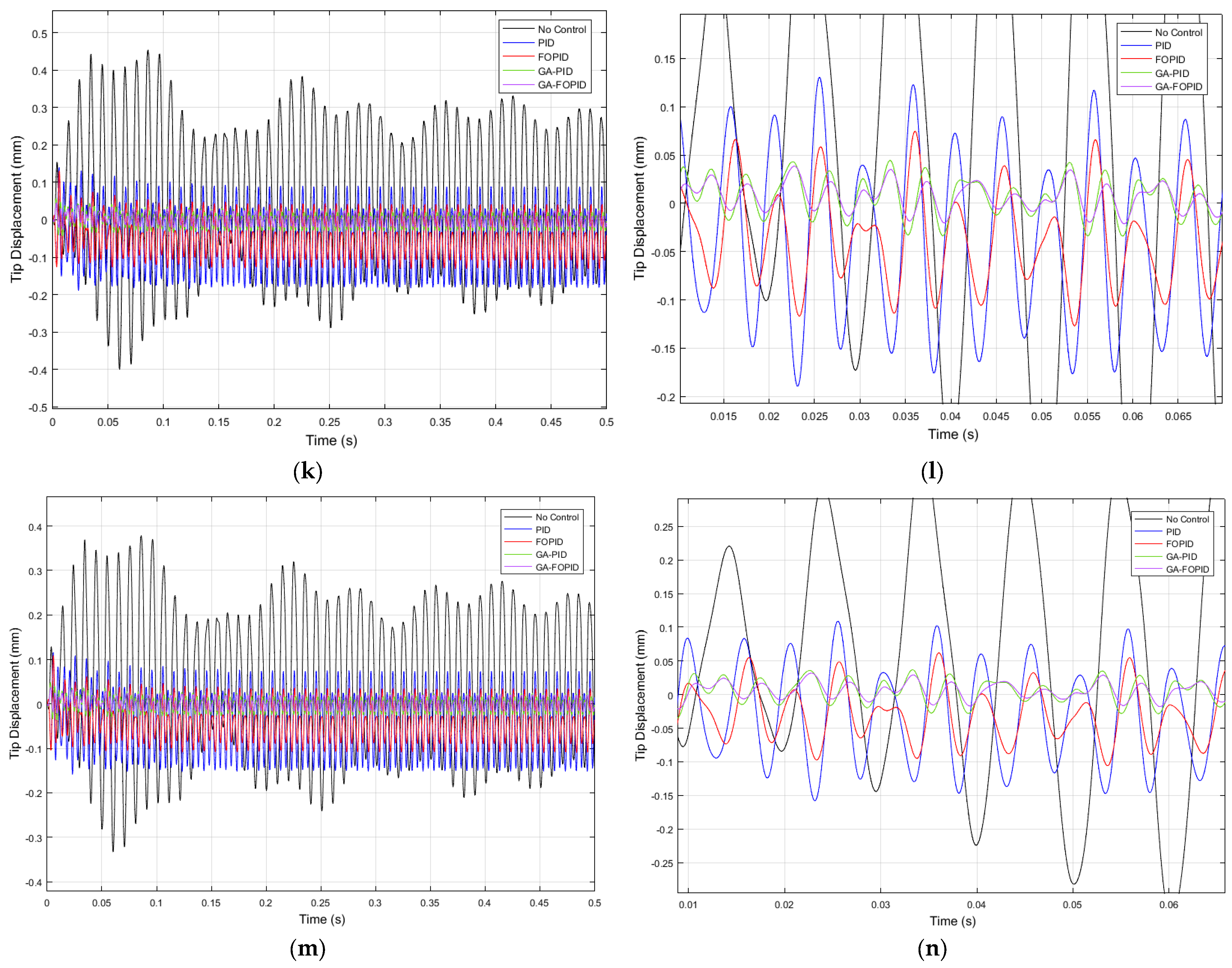
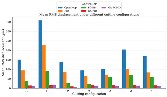
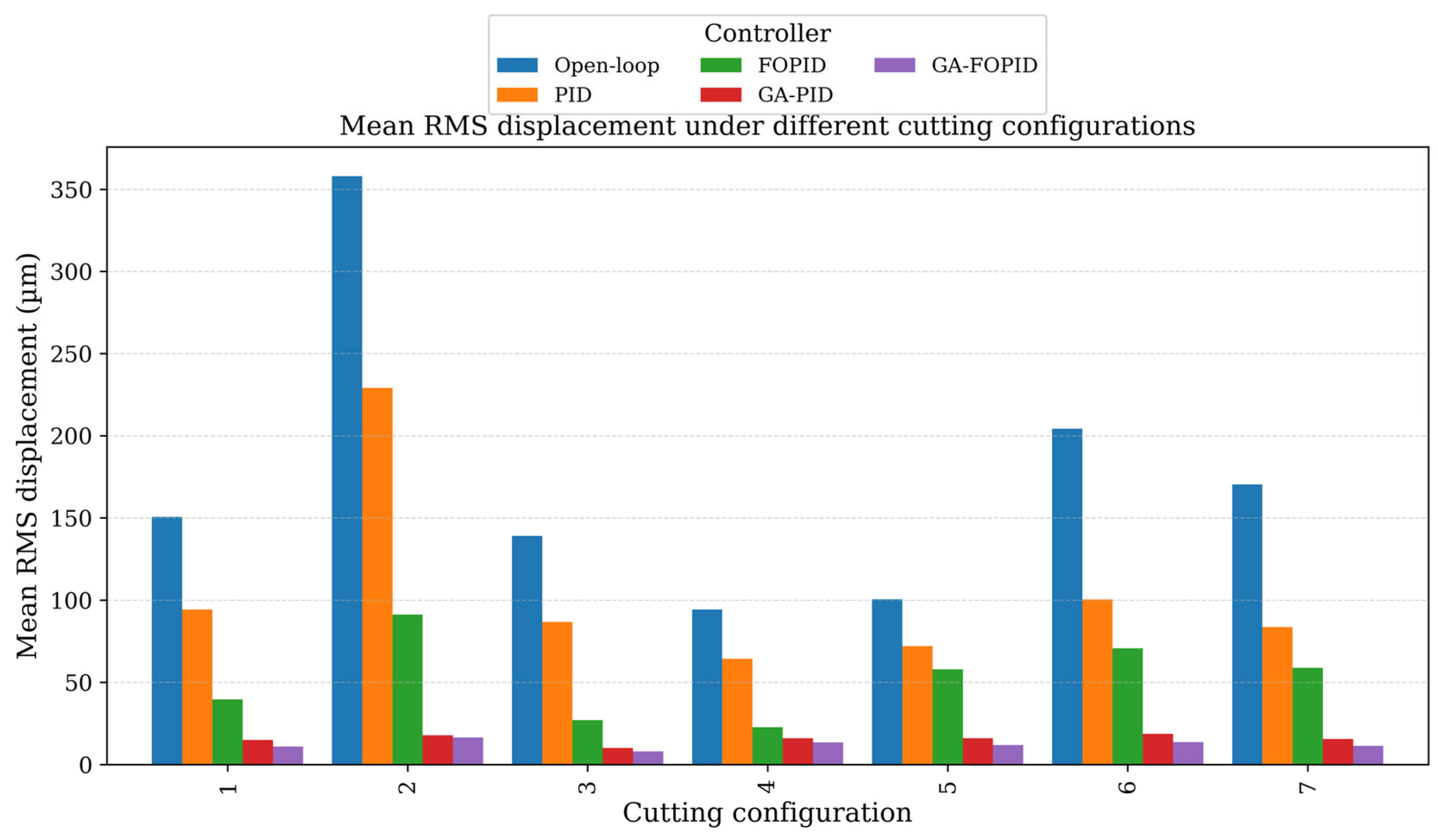
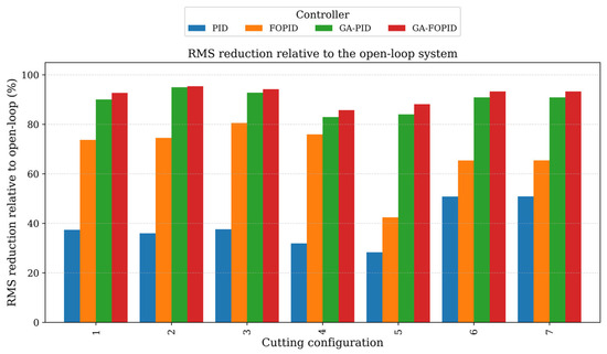
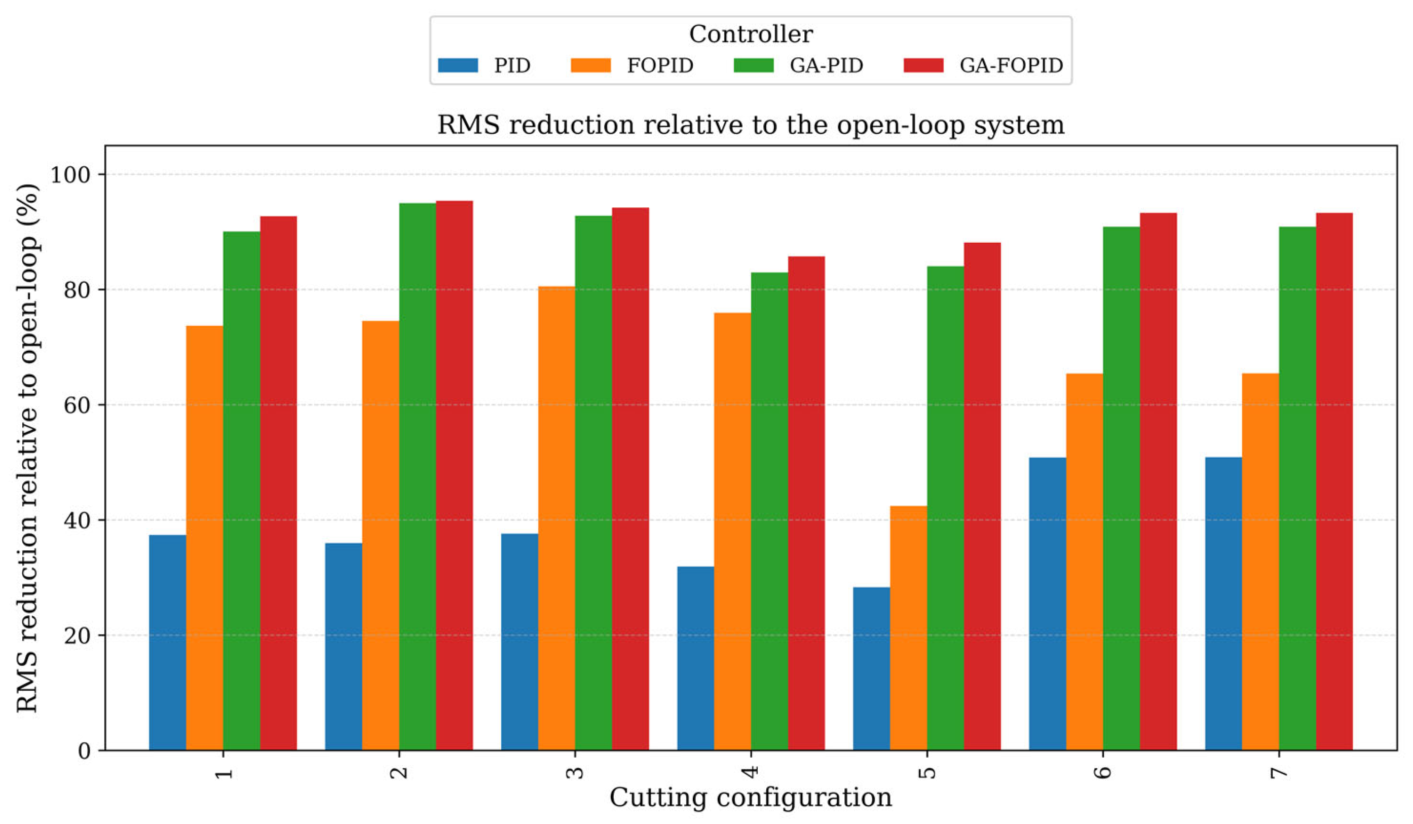
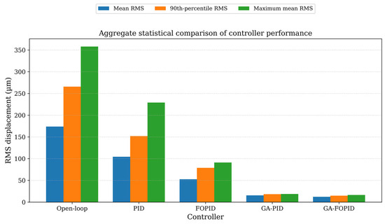
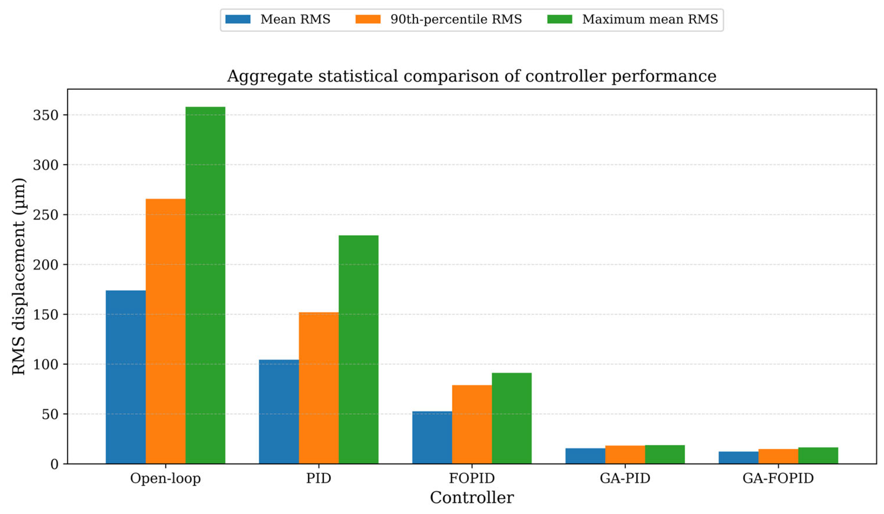

Disclaimer/Publisher’s Note: The statements, opinions and data contained in all publications are solely those of the individual author(s) and contributor(s) and not of MDPI and/or the editor(s). MDPI and/or the editor(s) disclaim responsibility for any injury to people or property resulting from any ideas, methods, instructions or products referred to in the content. |
© 2026 by the authors. Licensee MDPI, Basel, Switzerland. This article is an open access article distributed under the terms and conditions of the Creative Commons Attribution (CC BY) license.