A Novel Hybrid Approach for Non-Stationary Electricity Price Forecasting

Abstract

With the implementation of market-oriented electricity trading in an increasing number of countries, accurate electricity price forecasting can not only help participants in the electricity market to make more reasonable decisions but also enable regulators to have a more reliable regulatory basis. Therefore, it is necessary to propose an appropriate electricity price forecasting method. In view of the insufficiency of the traditional models in dealing with nonlinear and non-stationary data, to improve the detection ability of the model for hidden information in data and considering the high randomness of electricity price data, this paper proposes an electricity price forecasting method based on singular spectrum analysis (SSA) to decompose the original sequence and combines it with an extreme learning machine (ELM) optimized by the grey wolf optimizer (GWO). First, SSA is used to decompose the original sequence, and then the ELM is used to predict each subsequence and add them, in which the number of neurons in the hidden layer of each ELM is jointly optimized by the GWO. To verify the effectiveness of the SSA–GWO–ELM model, a total of 2106 days of electricity price data in Victoria, Australia, were selected for modeling. The results show that the prediction accuracy of the model proposed in this paper is significantly higher than that of the other comparison models, and the R² score is as high as 0.989, which is 0.017 higher than that of the suboptimal SSA–ELM. It can also maintain strong robustness and high prediction accuracy for heterogeneous data on power demand. SSA has the potential for real-time prediction, which can provide reliable data support for electricity market participants and supervisors.

1. Introduction

Currently, electricity market reform and competitive power trading have been promoted in several countries, including Australia, the United States, and Canada. In these markets, electricity prices are increasingly influenced by market competition rather than being determined solely by traditional monopoly regulation. In this context, accurate electricity price forecasting is highly important for producers, consumers, and regulators [1]. By forecasting the electricity price, consumers can dynamically arrange production to minimize the cost, while power generation enterprises can grasp the market trend in competition and then use the appropriate allocation strategy of both the quantity and price of electricity to bid for more profits. Moreover, for market supervisors, a good electricity price forecast can also provide a more scientific and reliable supervisory basis and better guarantee the normal and orderly operation of the electricity market. In addition, accurate forecasting models can also serve as important upstream modules for downstream operational decision-making and intelligent scheduling in complex industrial systems [2,3]. Currently, many experts and scholars have made continuous efforts in electricity price forecasting, and many methods have been proposed.

At present, the research methods used in electricity price forecasting can be roughly divided into three categories: econometric methods, machine learning methods, and decomposition–prediction strategies.

Econometric models, such as the autoregressive integrated moving average model (ARIMA) [4], the generalized autoregressive conditional heteroscedasticity model (GARCH) [5], and the combination of both models [6], are theoretically complete and highly interpretable. All these models have been applied to electric power research. However, most econometric methods are suitable for linear or weakly nonlinear problems and often have limited ability when dealing with highly nonlinear and non-stationary electricity price series. To capture more factors that affect electricity prices and improve prediction accuracy, many scholars have devoted themselves to establishing machine learning models to predict electricity prices, such as support vector machines (SVMs) [7], backpropagation neural networks (BPNNs) [8], and extreme learning machines (ELMs) [9]. Daviran M et al. [7] proposed a support vector machine based on time series segmentation, recursive feature elimination, and minimum redundancy maximum relevance (TSS–RFE–MRMR-based SVM). Principal component analysis dynamic programming (PCA–DP) was used to segment the time series, and the important features were selected via RFE–MRMR. Finally, the model was evaluated in the electricity markets of Ontario and New York, and it was found that the accuracy was better than that of other traditional methods. However, such methods still rely heavily on handcrafted feature selection and segmentation design, which may limit their robustness and generalizability across different market conditions. Considering the slow training speed of the BPNN and the ease of falling into a local optimum, Al-Haija Q A et al. [9] used an ELM for the rapid prediction of electricity prices. Compared with the BPNN, SVM and other models, the ELM can effectively capture nonlinearity from price series with high volatility, and the computing time is shorter. Nevertheless, the performance of the ELM is still sensitive to the selection of hidden-layer parameters, especially the number of hidden neurons. With the gradual development of deep learning in language processing, models such as recurrent neural networks (RNNs) and long short-term memory (LSTM) have begun to be used for sequence data other than language data. Usman M et al. [10] selected the parameters of the artificial neural network on the basis of mutual information and a decision tree, and the RNN-based prediction engine was used to predict the electricity load and price. The proposed method can improve the accuracy of electricity price prediction. Zhou S et al. [11] constructed a heterogeneous LSTM model and optimized its hyperparameters via sequence model-based optimization (SMBO). They then tested it on decomposed and reconstructed electricity price data, and the results revealed that the model outperformed both the general LSTM model and traditional models. Moreover, recent studies have shown that transformer-based and attention-enhanced deep architectures can model complex temporal and frequency-dependent patterns effectively in forecasting tasks [12,13]. Although these machine learning and deep learning methods have significantly improved predictive ability, their performance still often depends on feature engineering, hyperparameter tuning, and training stability. In addition, when directly applied to raw electricity price series, they may not sufficiently capture the multiscale fluctuation structures inherent in the data.

For non-stationary and highly random data, many researchers have further introduced decomposition–prediction strategies inspired by signal processing. The commonly used decomposition methods include empirical mode decomposition (EMD, EEMD, CEEMDAN, ICEEMDAN, etc.), local mean decomposition (LMD), wavelet packet transform (WPT), and singular spectrum analysis (SSA). After empirical mode decomposition (EMD) was used, He K et al. [14] modeled the downside risk of the electricity market with the exponentially weighted moving average (EWMA), and the results were better than those of a single EWMA model; Jiang X et al. [15] used the complete ensemble empirical mode decomposition with adaptive noise (CEEMDAN) method to decompose the PM_2.5 data sequence, reconstructed the subsequence according to the fuzzy entropy (FE) of the subsequence, and combined it with the bidirectional long short-term memory network (BiLSTM) for prediction. The “CEEMDAN–FE” strategy can effectively overcome noise and improve prediction performance. Sun W et al. [16] used EEMD to decompose the original carbon price and then used the wLSSVM optimized by LDWPSO to predict each sequence separately. Finally, the prediction results of each series were summed to obtain the final predicted value. The results show that EEMD and LDWPSO could significantly improve the forecasting performance. Although these decomposition methods have been widely used in forecasting risk [14], air pollution [15] and other fields, they are rarely used in electricity price forecasting. However, commonly used decomposition methods may still suffer from issues, such as mode mixing, sensitivity to noise, unstable component separation, or relatively high computational costs, in some settings. In addition, the overall forecasting pipeline may become more complex, and the final performance can depend strongly on the quality of decomposition.

The training of the ELM does not require cyclic iteration and takes less time, making it feasible for a heuristic algorithm to optimize its parameters. Cai W et al. [17] proposed the PSO–ELM model by combining the advantages of particle swarm optimization (PSO) in global search with the ELM in nonlinear learning and applied it to traffic flow prediction. However, PSO-based optimization may still suffer from issues such as premature convergence and sensitivity to parameter settings. Recent studies have shown that the grey wolf optimizer (GWO) and its variants have also achieved strong performance in complex optimization tasks, such as controller tuning, scheduling, and energy system coordination [18,19,20]. Vautard R et al. [21] noted that SSA is a powerful descriptive tool that can describe general nonlinear dynamics, especially climate dynamics. However, few studies have applied SSA to electricity price forecasting. In addition, ELMs have fast forecasting ability and strong generalization ability. Therefore, to better exploit the advantages of decomposition and learning-based prediction while alleviating the above limitations, this paper constructs an SSA–GWO–ELM model according to the “decomposition–prediction” strategy, in which the GWO is used to optimize the hidden-layer neuron number of the ELM. The proposed model is compared with benchmark models on the electricity price dataset of Victoria, Australia.

2. Research Methods

2.1. SSA

Singular spectrum analysis (SSA) is a decomposition method proposed by Colebrook [22] that can effectively decompose low-frequency trend sequences, strong periodic sequences, and high-frequency noise sequences. It is suitable for nonlinear and non-stationary sequences.

The execution steps of SSA are as follows:

(1)

Constructing the trajectory matrix: According to the preset embedding dimension $L$, embed the time series data $X=(x_1,\cdots ,x_N)$ of length $N$ to obtain the trajectory matrix $T$:

$$T=\left(\begin{array}{ccc}{x}_1& \cdots & x_K\\ ⋮& & ⋮\\ x_L& \cdots & x_N\end{array}\right)$$

(1)

where $K=N-L+1$.

(2)

Singular value decomposition: Singular value decomposition is performed on the trajectory matrix $T$ to obtain $T_{L\times K}=U_{L\times L}\Sigma V_{K\times K}^{\top }$. Let $s$ be the number of nonzero singular values; then, $T_{L\times K}$ can also be expressed as

$$T=\sum _{i=1}^s{T}_i$$

(2)

where $T_i=\sqrt{{\lambda }_i}{U}_i{V}_i^{\top }$ and where ${\lambda }_i$ is the i-th largest eigenvalue of $T{T}^{\top }$.

(3)

Grouping: The index set $\{1,2,\cdots ,s\}$ is partitioned into d disjoint subsets $C_1,\cdots ,C_d,(d\le s)$ according to a predefined strategy. If $C_j=\{C_{j1},C_{j2},\cdots ,C_{j{n}_j}\}$, then the original index set can be expressed as

$$\left\{1,2,\cdots ,s\right\}=\left\{C_{11},\cdots ,C_{1n_1},C_{21},\cdots ,C_{2n_2},\cdots ,C_{d1},\cdots ,C_{d{n}_d}\right\}$$

(3)

The matrices in each subscript subset $T_{C_j}$ are added to obtain $C_j$; in this way, Formula (2) can also be written as

$$T=\sum _{j=1}^d{T}_{C_j}=\sum _{j=1}^d\sum _{i=1}^{n_j}{T}_{C_{ji}}$$

(4)

(4)

Reconstruction based on the diagonal averaging method: For each grouped trajectory matrix $T_{C_j}$, the diagonal averaging method can be used to reduce it to time series data. The specific way to reduce the matrix $T_{C_j}={\left(t_{ij}\right)}_{L\times K}$ to time series data $x_{C_j}=({\widehat{x}}_{j1},{\widehat{x}}_{j2},\cdots ,{\widehat{x}}_{jN})$ is as follows:

$${\widehat{x}}_{jk}=\{\begin{array}{c}{\displaystyle \frac{1}{k}}{\displaystyle \sum _{i=1}^k}{t}_{i,k-i+1,\hspace{1em}\hspace{1em}\hspace{1em}\hspace{1em}\hspace{1em}\hspace{1em}\hspace{1em}\hspace{1em}}1\le k\le L^{*}\\ {\displaystyle \frac{1}{L^{*}}}{\displaystyle \sum _{i=1}^{L^{*}}}{t}_{i,k-i+1},\hspace{1em}\hspace{1em}\hspace{1em}\hspace{1em} L^{*}\le k\le K^{*}\\ {\displaystyle \frac{1}{N-k+1}}{\displaystyle \sum _{i=k-K^{*}+1}^{N-K^{*}+1}}{t}_{i,k-i+1},K^{*}\le k\le N\end{array}$$

(5)

where $L^{*}=\min \{L,K\}$, $K^{*}=\max \{L,K\}$, and, finally, we obtain the decomposition of the original time series data $X=(x_1,x_2,\cdots ,x_N)$:

$$x_i=\sum _{j=1}^d{\widehat{x}}_{ji},i=1,2,\cdots ,N$$

(6)

2.2. The GWO

The grey wolf optimizer (GWO) is a swarm intelligence optimization algorithm that mimics the leadership hierarchy and hunting behavior of grey wolves [23]. In the standard GWO framework, the three best candidate solutions are denoted as alpha (α), beta (β), and delta (δ), which guide the remaining wolves to update their positions toward promising regions of the search space [23]. Recent studies have shown that the GWO and its variants have achieved strong performance in complex optimization tasks, such as controller tuning, scheduling, and energy system coordination, which supports its use in optimizing the hidden-layer neuron number of the ELM in this study [18,19,20]. For the optimization problem considered in this paper, each wolf represents a candidate number of hidden neurons in the ELM, and the RMSE on the validation set is adopted as the fitness value. The position update process can be expressed as follows [23]:

$$D_{\alpha }=\left|C_1{X}_{\alpha }-X\right|$$

(7)

$$D_{\beta }=\left|C_2{X}_{\beta }-X\right|$$

(8)

$$D_{\delta }=\left|C_3{X}_{\delta }-X\right|$$

(9)

$$X_1=X_{\alpha }-A_1{D}_{\alpha }$$

(10)

$$X_2=X_{\beta }-A_2{D}_{\beta }$$

(11)

$$X_3=X_{\delta }-A_3{D}_{\delta }$$

(12)

$$X(t+1)={\displaystyle \frac{X_1+X_2+X_3}{3}}$$

(13)

where X denotes the current position of a wolf, and $X_{\alpha }$, $X_{\beta }$, and $X_{\delta }$ denote the positions of the α, β and δ wolves, respectively. $A=2a{r}_1-a$, $C=2r_2$, $r_1$ and $r_2$ are random vectors in [0, 1], and a decreases linearly from 2 to 0 during the iterative process [23]. Since the number of hidden-layer neurons is an integer variable, each wolf position is rounded to the nearest integer and clipped to the predefined search range before fitness evaluation. In this work, the GWO is used to search for the optimal hidden-layer neuron number of each ELM predictor to improve the forecasting performance.

2.3. ELM

The extreme learning machine (ELM) is a kind of single-layer feedforward neural network (SLFN). Considering that the parameter estimation of a conventional BP neural network needs to go through many iterations and that it is easy to fall into the local optimal solution, Huang G et al. [24] proposed an ELM based on generalized inverse matrix theory. During training, the weights are estimated by solving the generalized inverse matrix. The training time is shorter, and the generalization ability is stronger.

For sample $\mathcal{D}=\left\{\left(x_1,t_1\right),\left(x_2,t_2\right)\cdots ,\left(x_Q,t_Q\right)\right\}$, where $\left(x_j,t_j\right)\in ({\mathbb{R}}^m,{\mathbb{R}}^n)$ and $j=1,\cdots ,Q$, the feature dimensions of the input layer and the output layer are denoted as $m,n$, respectively. Let $w_{ij}$ be the weight between the i-th input neuron and the j-th hidden-layer neuron, denoted as $\mathit{w}={\left(w_{ij}\right)}_{m\times l}$. Let ${\beta }_{ij}$ be the weight between the i-th hidden-layer neuron and the j-th output neuron, denoted as $\mathit{\beta }={\left({\beta }_{ij}\right)}_{l\times n}$. If the activation function of the hidden layer is denoted as $f$ and the bias term is $\mathit{b}=\left(b_1,\cdots ,b_l\right)$, the hidden layer for sample $x_j$ can be expressed as

$$h_{ji}=f\left(w_i^{\top }{x}_j+b_i\right),i=1,\cdots ,l$$

(14)

where $w_i$ represents the i-th column vector of matrix $\mathit{w}$, and the output layer for sample $x_j$ can be expressed as

$$t_{ji}=\sum _{k=1}^l{\beta }_{ki}{h}_{jk}=\sum _{k=1}^l{\beta }_{ki}f\left(w_k^{\top }{x}_j+b_k\right),i=1,\cdots ,n$$

(15)

For sample $D$, the output of the ELM is as follows:

$$T{=\left(t_1,\cdots ,t_Q\right)}^{\top }=\left(\begin{array}{ccc}{t}_{11}& \cdots & t_{1n}\\ ⋮& & ⋮\\ t_{Q1}& \cdots & t_{Qn}\end{array}\right)$$

(16)

The element in $T$ is determined via Formula (15) if the following expression is used:

$$\mathit{H}=\left(\begin{array}{ccc}f\left(w_1^{\top }{x}_1+b_1\right)& \cdots & f\left(w_l^{\top }{x}_1+b_l\right)\\ ⋮& & ⋮\\ f\left(w_1^{\top }{x}_Q+b_1\right)& \cdots & f\left(w_l^{\top }{x}_Q+b_l\right)\end{array}\right)$$

(17)

Then, Formula (16) can be written in matrix form: $T=\mathit{H}\mathit{\beta }$.

The ELM randomly sets parameters $\mathit{w}$ and $\mathit{b}$ before training; that is, $\mathit{H}$ is known. Therefore, according to the label $T$, the parameter $\mathit{\beta }={\mathit{H}}^{†}T$ can be obtained, where ${\mathit{H}}^{†}$ is the generalized inverse matrix of $\mathit{H}$. In the present implementation, no additional explicit regularization term was introduced into the ELM. This choice was made to keep the model structure simple and to isolate the contribution of the decomposition strategy and the swarm-intelligence-based hyperparameter optimization. Instead, model complexity was controlled mainly by the number of hidden-layer neurons, the sliding-window setting, and the chronological validation procedure.

2.4. SSA–GWO–ELM

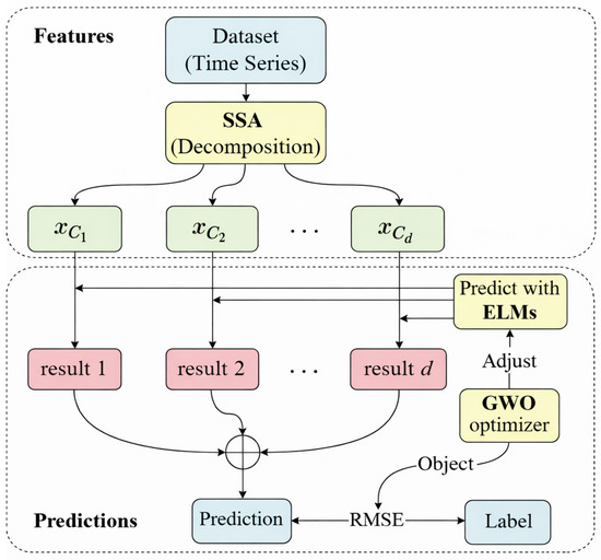
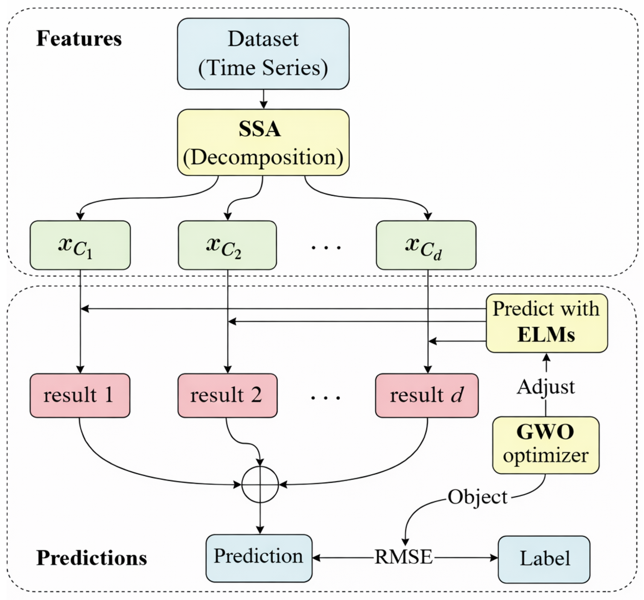
The idea of the prediction model is “decomposition–prediction–integration”. First, the original electricity price data sequence is decomposed with SSA, the ELM model is used to predict each subsequence decomposed, and, finally, the predicted value of each subsequence is added to obtain the final predicted value. When determining the number of neurons in the hidden layer of each ELM, the GWO algorithm is employed for hyperparameter search. Specifically, each wolf represents a candidate hidden-layer neuron number, and the validation RMSE is adopted as the fitness value. The candidate yielding the minimum validation RMSE is selected as the final configuration for the corresponding ELM predictor. The overall model architecture is shown in Figure 1.

Figure 1. SSA–GWO–ELM model flowchart.

3. Analysis of the SSA–GWO–ELM Model in Electricity Price Forecasting

3.1. Data Sources

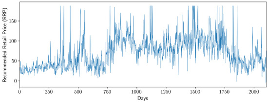
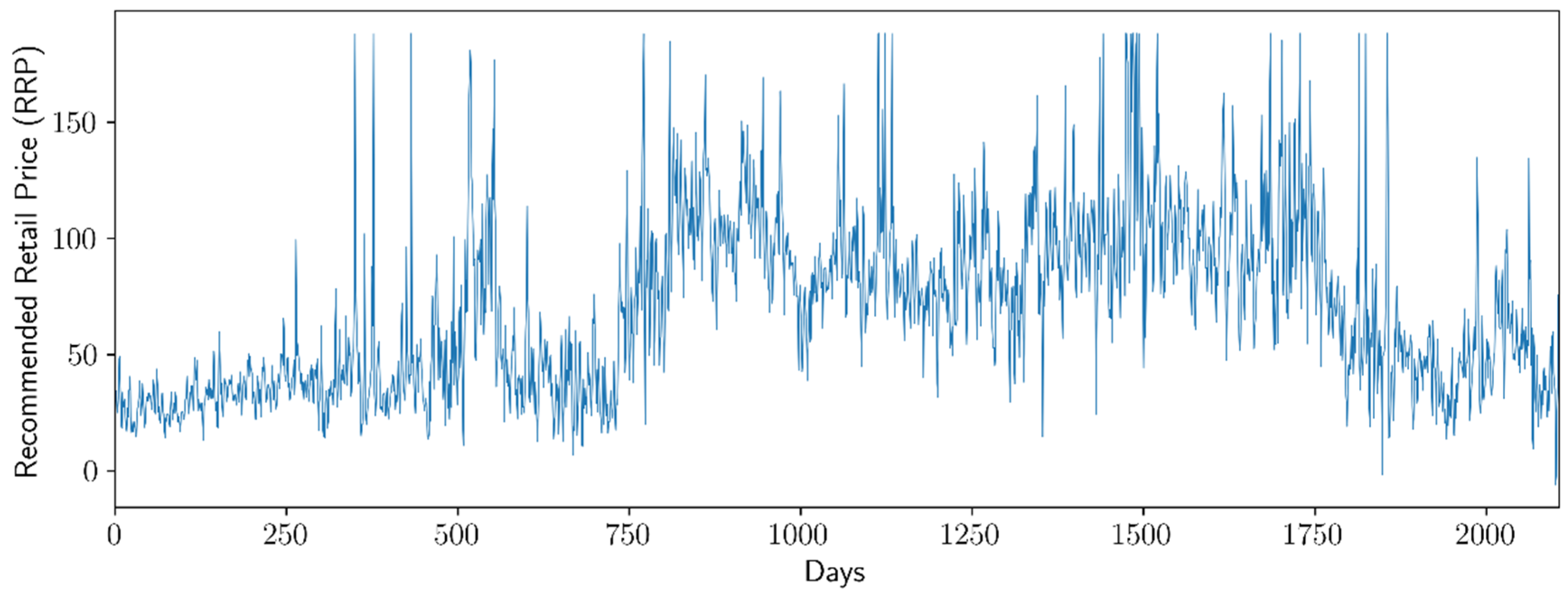
The experiment selects electricity price data from 1 January 2015 to 6 October 2020 in Victoria, Australia, from the Daily Electricity Price and Demand Data dataset on Kaggle (https://www.kaggle.com/aramacus/electricity-demand-in-victoria-australia, accessed on 20 April 2026), for a total of 2106 entries. There are no missing values in the data selected in the experiment, but there are extreme values. In this way, during training, the model tends to focus on the prediction of extreme values to decrease the total prediction error. Moreover, this approach decreases the prediction of nonextreme values. Therefore, the prediction accuracy is reduced. Owing to the small proportion of extreme values and the preservation of the original information as much as possible, the 99th quantile capping method is used in preprocessing, and the processed data sequence is shown in Figure 2.

Figure 2. Daily RRP value (AUD/MWh).

3.2. Parameter Settings

For fair comparison, all the baseline and decomposition-based models used the same chronological data split, the same sliding-window reconstruction strategy, and the same evaluation metrics. For the GWO-based models, only the hidden-layer neuron number of the ELM was optimized, whereas the other settings were kept fixed across the models. For the data above, the following parameter settings are chosen:

(1)

SSA parameter setting: While grouping, each eigenvalue is selected as a group; that is, $d=s$ is chosen.

(2)

GWO parameter setting: According to the scale of the dataset, the search interval of the hidden-layer neuron number for each ELM is set to [5, 120]. The population size and maximum iteration number of the GWO are set to 30 and 50, respectively. These settings were determined based on preliminary experiments and empirical experience, with consideration of the trade-off between forecasting performance and computational cost. During optimization, the fitness value is defined as the RMSE of the corresponding ELM predictor.

(3)

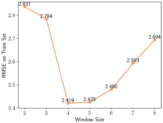
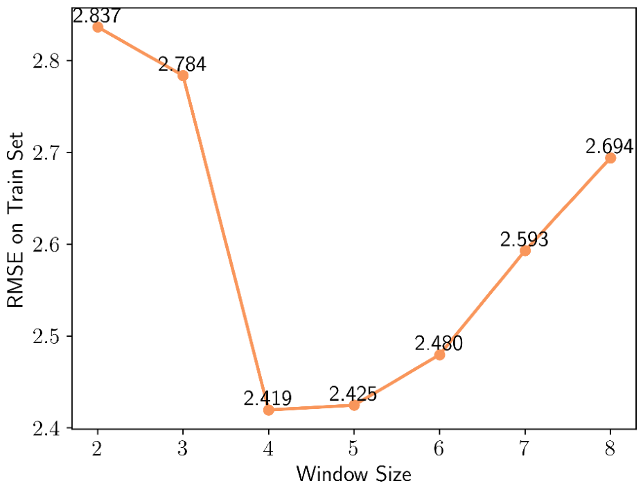
ELM parameter setting: Modeling was implemented in Python 3.8.10 using the hpelm package [25]. The main software environments included hpelm 1.0.10, NumPy 1.24.3, SciPy 1.10.1, Pandas 1.5.3, and Scikit-learn 1.3.0. The training batch size was set to 20. We use the sliding window for feature construction during prediction. If the number of windows is selected as $w$, the decomposed data of the previous $w$ days are used as the input to predict the corresponding data of today. That is, the number of input neurons is selected as $w$, and the number of output neurons is 1. Specifically, the model prediction effect changes with the value of $w$, as shown in Figure 3, so $w=4$ is selected in this experiment.

Figure 3. Effect of window size on the model effect.

(4)

The dataset is reconstructed according to the sliding-window value, and $n=N-w+1=2101$ pieces of data are obtained. The first 80% were used for model development, including predictor construction and hyperparameter selection, and the remaining 20% were used as the held-out test set after sliding-window reconstruction. The training portion covered 5 January 2015–12 August 2019, and the held-out test set covered 13 August 2019–6 October 2020. Since the ELM does not rely on iterative backpropagation, there is no epoch-wise training schedule, as in gradient-based neural networks. Instead, the training-validation procedure is carried out in an iteration-wise manner during GWO: at each GWO iteration, each wolf encodes a candidate hidden-layer neuron number, the corresponding ELM is trained on the sub-training set, and its validation RMSE is computed as the fitness value. After the search process is complete, the best hidden-layer neuron number is selected according to the minimum validation RMSE, and the final model is retrained on the whole training portion and evaluated on the held-out test set.

Four evaluation metrics, namely the MAE, RMSE, SMAPE, and R², are adopted to evaluate model performance from different perspectives. The MAE measures the average magnitude of the forecasting errors in the original unit of the data. The RMSE assigns a larger penalty to large deviations and is therefore particularly suitable for highly volatile electricity price series. SMAPE is a scale-independent percentage error metric that facilitates comparisons across datasets with different magnitudes, such as electricity price and electricity demand. R² measures the goodness of fit and reflects the proportion of variance in the target series explained by the model.

3.3. Data Decomposition and Parametric Search

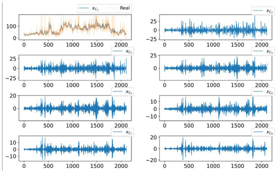
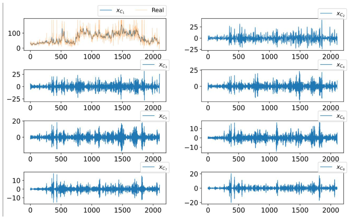
Considering that the numbers of subsequences decomposed via the comparative decomposition method and the LMD and EMD-class decomposition methods are 7 and 9, respectively, to avoid excessive discrepancies in data volume, the embedding dimension $L$ of SSA is selected to be 8, and the 8 subsequences decomposed via this method are shown in Figure 4.

Figure 4. Decomposition results of SSA.

In particular, the image of the original data is also shown in the image of the subsequence $x_{C_1}$ corresponding to the largest eigenvalue in Figure 4. $x_{C_1}$ represents the trend of the sequence well. The frequency of the subsequent decomposition sequences increases, and their regularity decreases. Moreover, the information represented by the subsequences tends to be noise.

After decomposing the subsequences, we use the ELM optimized by the GWO to predict each subsequence separately. For each subsequence, the hidden-layer neuron number is selected according to the minimum validation RMSE. Robustness is not used as the direct optimization objective; instead, it is assessed separately by the standard deviation over 50 independent runs. The optimal numbers of hidden-layer neurons identified via the GWO are shown in Table 1.

Table 1. Optimal number of neurons in the hidden layer of the ELMs searched by GWO.

$\mathbf{Subsequence}{\mathit{x}}_{{\mathit{C}}_{\mathit{j}}}$	Number of Neurons	$\mathbf{Subsequence}{\mathit{x}}_{{\mathit{C}}_{\mathit{j}}}$	Number of Neurons
$x_{C_1}$	99	$x_{C_5}$	108
$x_{C_2}$	98	$x_{C_6}$	5
$x_{C_3}$	115	$x_{C_7}$	119
$x_{C_4}$	89	$x_{C_8}$	69

3.4. Model Comparison Analysis

3.4.1. Comparison of Decomposition Methods

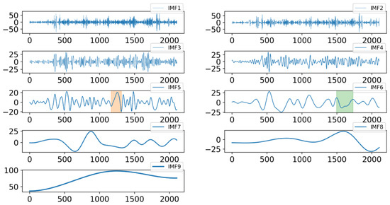
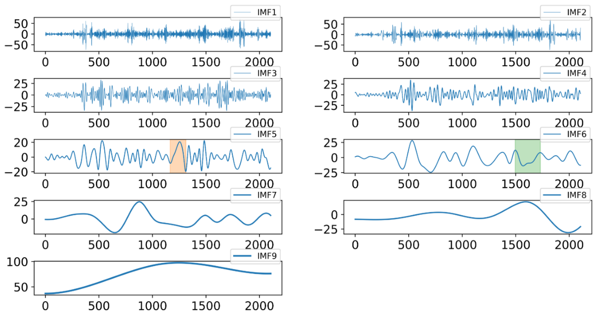
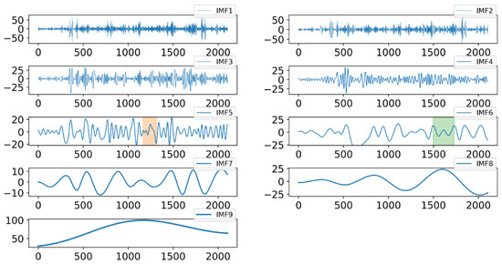
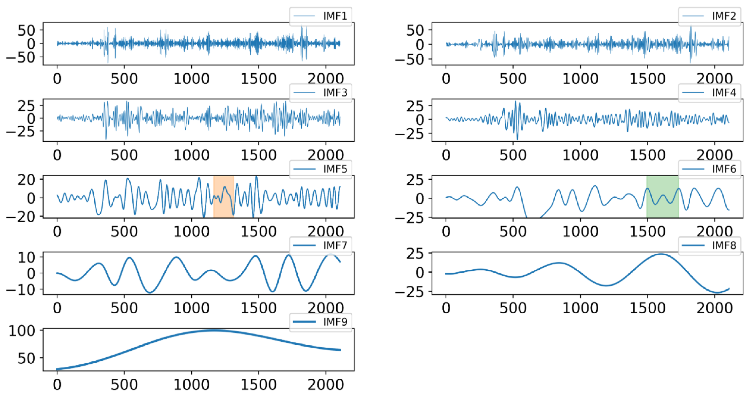
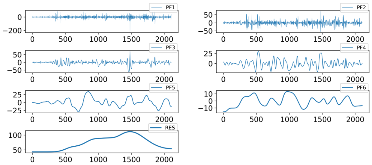
The decomposition results of different decomposition methods differ in the frequency of subsequences. Figure 4, Figure 5, Figure 6 and Figure 7 show the subsequences decomposed by SSA, EMD, CEEMDAN and LMD, respectively.

Figure 5. Decomposition results of EMD. Different colors are used only to distinguish different decomposed components. The shaded region indicates the typical fluctuation interval selected in this study, which is highlighted to more clearly show the amplitude variation and frequency characteristics of the corresponding IMF components during this period compared with the overall series.

Figure 6. Decomposition results of CEEMDAN. Different colors are used only to distinguish different decomposed components. The shaded region indicates the typical fluctuation interval selected in this study, which is highlighted to more clearly show the amplitude variation and frequency.

Figure 7. Decomposition results of LMD.

Figure 5 and Figure 6 report that the CEEMDAN decomposition method partially overcomes the mode mixing problem in the EMD method; that is, it partially avoids the same time scale appearing in different subsequences (such as the highlighted parts of IMF₅ and IMF₆ in the two figures). Moreover, the frequency of subsequences decomposed by EMD-class methods (such as EMD and CEEMDAN) and the LMD method decreases significantly from high to low, and a large gap in the amount of information between subsequences exists, which may cause the model to overfit noisy sequences with high frequency. The trend items represented by low-frequency sequences are not obvious, which is not conducive to model extraction of trend features.

With the exception of the first subsequence corresponding to the largest eigenvalue of the sequence decomposed by SSA, the frequency gap of the remaining subsequences is relatively small. Compared with the original data, the first subsequence can extract the trend information well, and its trend is well matched with the original sequence.

3.4.2. Comparison of Combined Models

To further verify the effectiveness of the proposed SSA–GWO–ELM model, classical decomposition methods, including EMD, CEEMDAN, and LMD, are selected for comparison, and the contribution of the GWO in model tuning is evaluated. For all the models, the above parameter settings are adopted, and the MAE, RMSE, SMAPE, and R² are used to evaluate the forecasting performance from the perspectives of absolute error, large-error sensitivity, relative percentage error, and overall goodness of fit, respectively. The efficiency of each decomposition method is evaluated by its decomposition time. To reduce the contingency caused by random initialization, each model is independently run 50 times, and the mean result is reported as the final performance. In addition, the standard deviation (SD) over 50 runs is reported to reflect robustness, whereas the p value is used to examine whether the improvement in each GWO-based model over its corresponding non-GWO counterpart is statistically significant.

From Table 2 and Figure 8, Figure 9 and Figure 10, the following observations can be made.

Table 2. Performance comparison of ELM-based forecasting models with different decomposition methods and GWO optimization on the Victoria electricity price dataset (mean over 50 runs).

Model	MAE	RMSE	SMAPE/(%)	R2	SD	p Value	Decompose Time/(s)
ELM	15.659	22.930	26.568	0.537	0.324	-	-
GWO–ELM	15.655	22.959	26.598	0.535	0.285	0.190	-
EMD–ELM	14.640	20.141	26.106	0.521	11.859	-	0.035
EMD–GWO–ELM	10.806	15.748	19.908	0.780	1.103	1.48 × 10−6	0.035
LMD–ELM	12.218	18.566	21.069	0.696	0.425	-	0.644
LMD–GWO–ELM	11.999	18.243	20.860	0.707	0.474	3.50 × 10−3	0.644
CEEMDAN–ELM	10.799	15.931	19.239	0.776	0.520	-	6.790
CEEMDAN–GWO–ELM	10.253	15.292	18.460	0.794	0.494	3.56 × 10−8	6.790
SSA–ELM	3.378	5.595	6.949	0.972	0.450	-	0.181
SSA–GWO–ELM	2.477	3.573	5.346	0.989	0.117	1.96 × 10−32	0.181

Figure 8. Comparison of the MAEs and RMSEs.

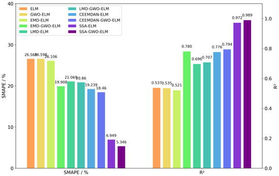
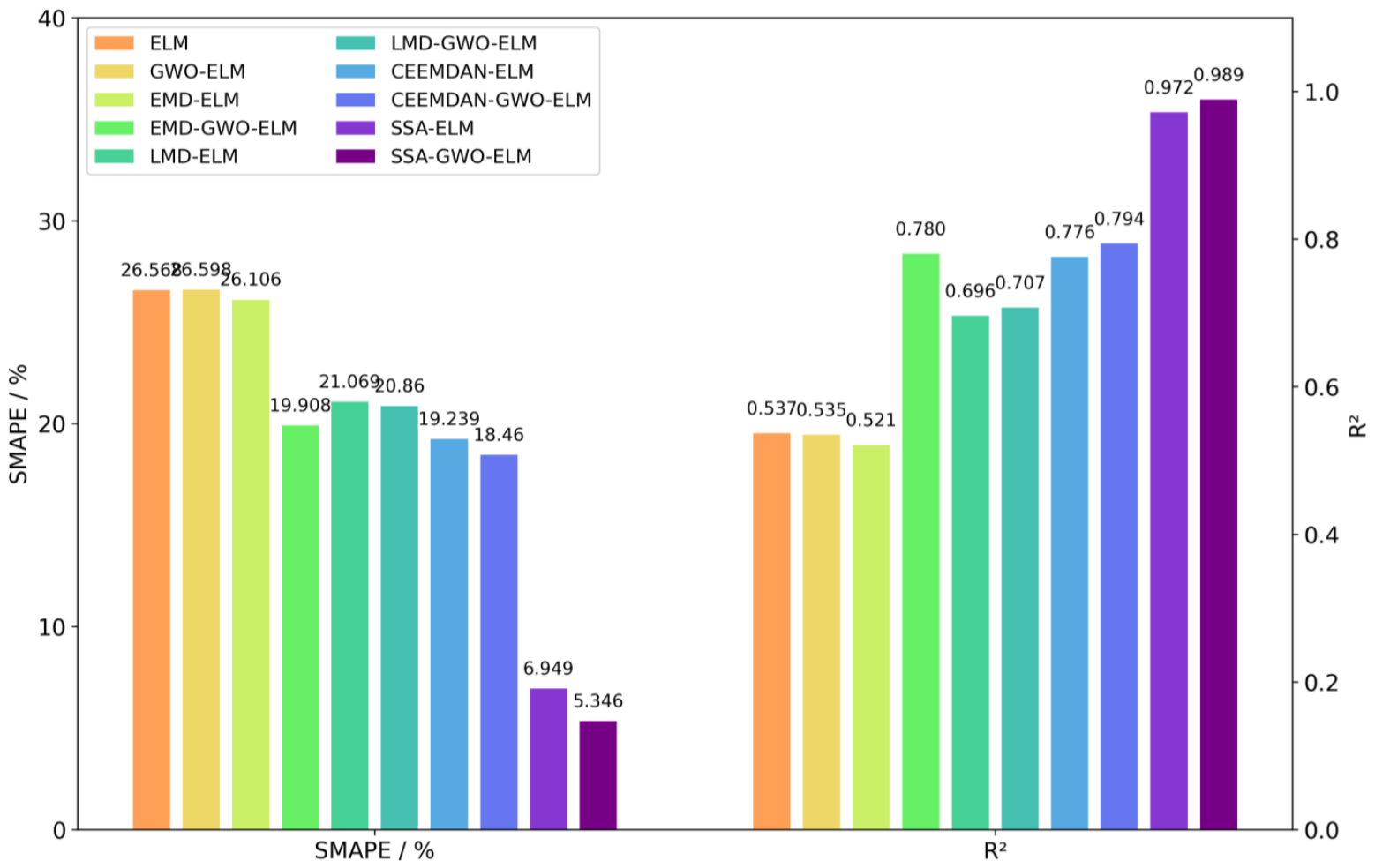
Figure 9. Comparison of SMAPE and R².

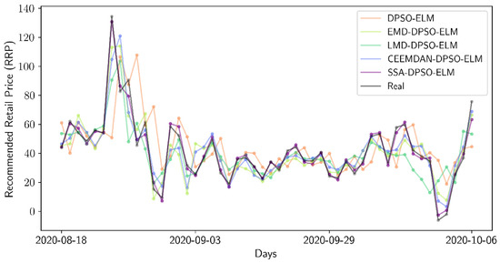
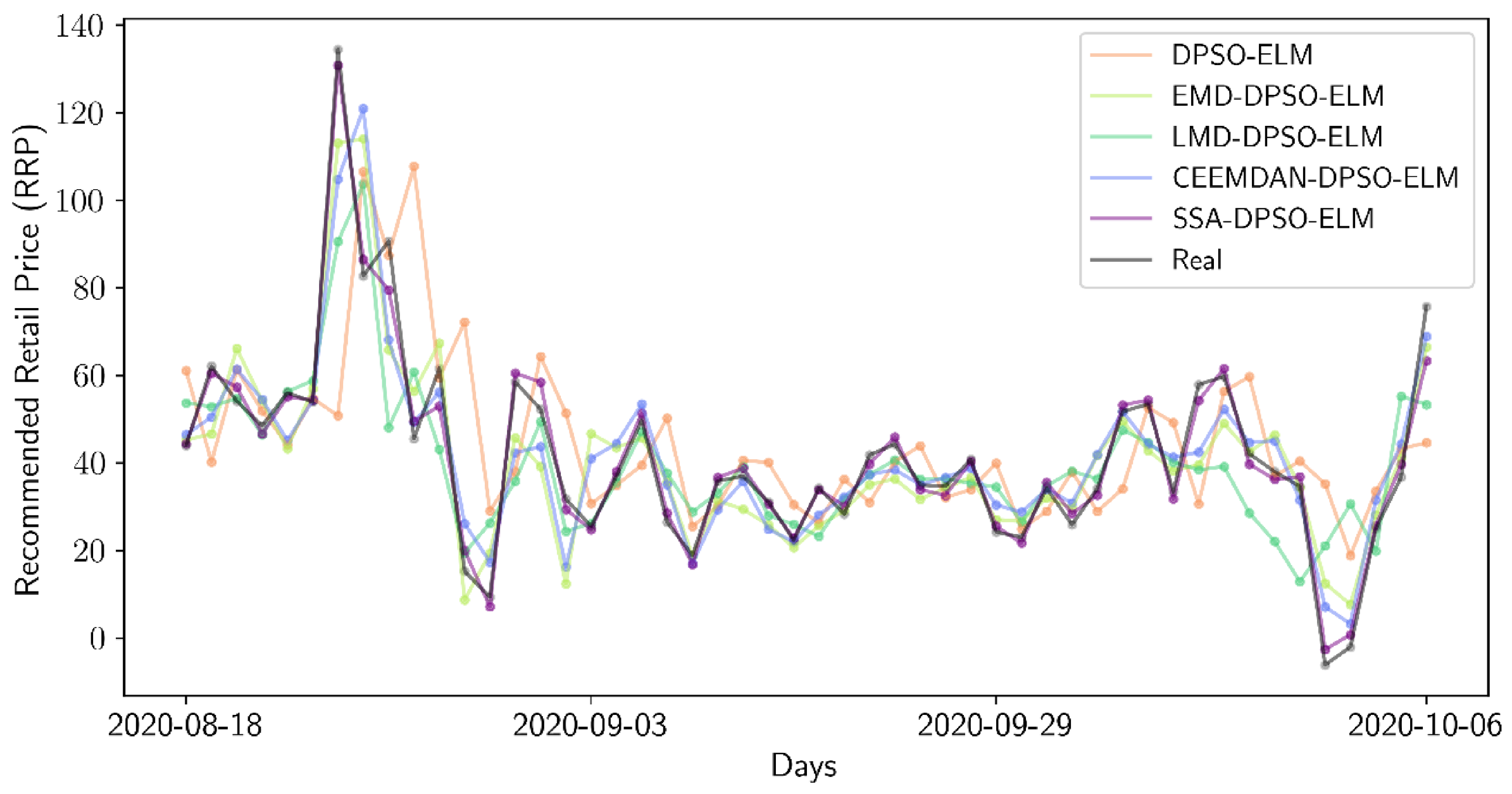
Figure 10. Display of the prediction performance of partial models in the last 50 days.

(1) The undecomposed ELM and GWO–ELM models achieve the weakest performance on the electricity price dataset. The R² values remain at approximately 0.54, indicating limited explanatory ability for the highly volatile raw price series. Moreover, the GWO does not clearly improve the undecomposed ELM baseline, suggesting that optimizer-only tuning is insufficient when the original series is not decomposed.

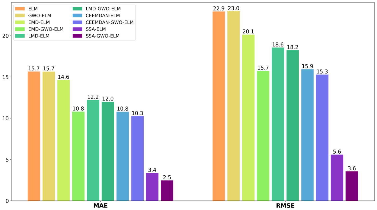
(2) Decomposition-based models generally improve forecasting performance. Compared with the ELM, the EMD–ELM, LMD–ELM, CEEMDAN–ELM, and SSA–ELM reduce the RMSE from 22.930 to 20.141, 18.566, 15.931, and 5.595, respectively. This indicates that decomposition helps to separate the original price series into components with different frequencies and structures, enabling the ELM to capture more informative patterns and improving the generalization ability. Among these methods, SSA provides the greatest improvement.

(3) The GWO further improves most decomposition-based ELM models. For example, compared with their corresponding nonoptimized counterparts, the RMSE values of the EMD–GWO–ELM, LMD–GWO–ELM, CEEMDAN–GWO–ELM, and SSA–GWO–ELM are further reduced to 15.748, 18.243, 15.292, and 3.573, respectively. The corresponding p values are all less than 0.01, indicating that the performance gains resulting from the GWO are statistically significant for these decomposition-based models.

(4) Among all the compared methods, SSA–GWO–ELM achieves the best overall performance, with an MAE of 2.477, an RMSE of 3.573, an SMAPE of 5.346%, and an R² of 0.989. Compared with the SSA–ELM, the GWO reduces the RMSE by approximately 36.14% and decreases the standard deviation (SD) from 0.450 to 0.117, which indicates that the proposed optimization strategy improves both the accuracy and robustness when combined with SSA-based decomposition. In addition, the R² of the SSA–GWO–ELM model is 0.195 greater than that of the best competing decomposition-based model, the CEEMDAN–GWO–ELM (R² = 0.794).

(5) In terms of decomposition efficiency, EMD is the fastest method, requiring only 0.035 s, whereas CEEMDAN is the most time-consuming, requiring 6.790 s. SSA requires only 0.181 s, which is slightly slower than EMD but substantially faster than CEEMDAN and still much faster than LMD. Considering both the forecasting accuracy and computational cost, SSA provides the best trade-off among the compared decomposition methods and therefore shows strong potential for real-time electricity price forecasting.

4. Generalization of the SSA–GWO–ELM Model in Electric Power Forecasting

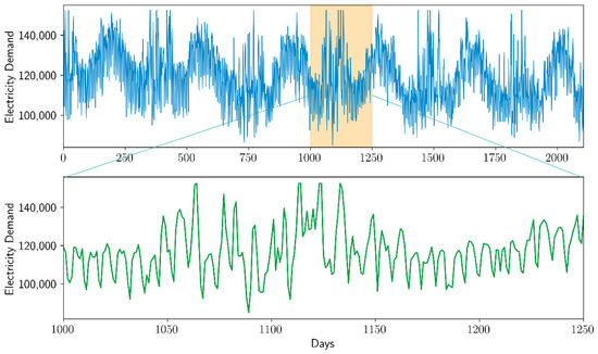
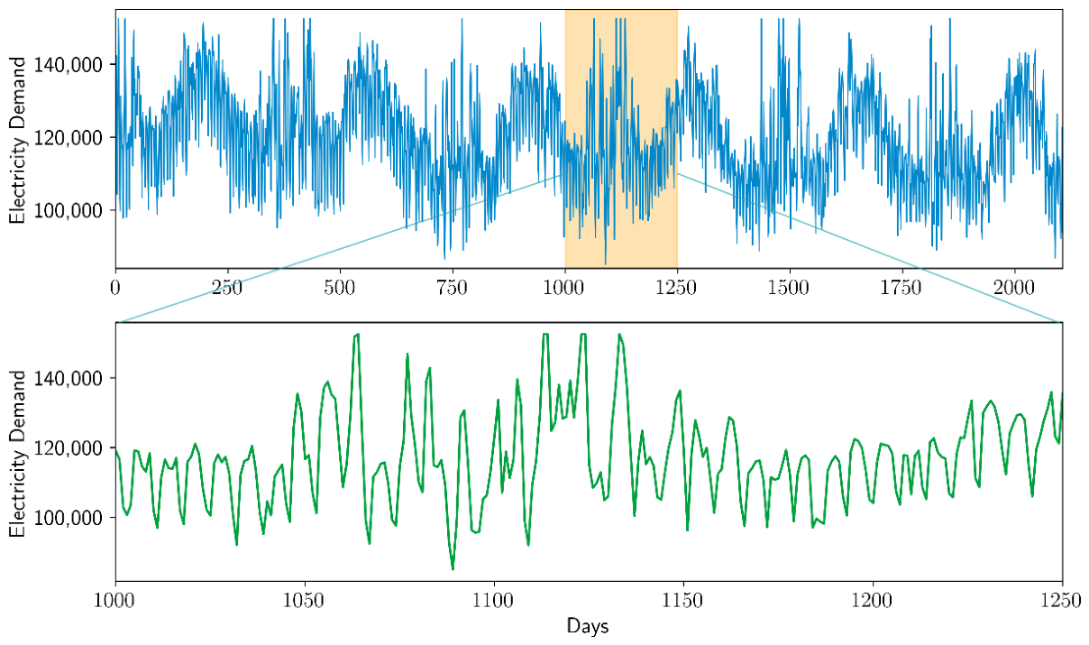
To further test the prediction performance of the proposed SSA–GWO–ELM model in other application scenarios of the electricity market, in this paper, the electricity demand data of 2106 entries from 1 January 2015 to 6 October 2020 in Victoria, Australia, under the same dataset are selected to retrain the models. In addition, predictions are made on this dataset. The power demand data are shown in Figure 11.

Figure 11. Overall visualization and partial enlarged view of the power demand series. The shaded area in the upper panel marks the representative interval selected for detailed observation, and the corresponding local pattern is displayed in the lower panel.

The electricity demand data are quite different from the previous electricity price data. Relatively speaking, the previous electricity price data are less periodical and more random, whereas the electricity demand data are the opposite. As shown in Figure 11, its periodicity can be roughly described as “major cycle” among years and “minor cycle” among weeks.

In the prediction, the same hyperparameter settings as those used previously are used, and the model is retrained, in which the optimal sliding-window size for SSA is $w=6$. The EMD, CEEMDAN, and LMD decomposition methods are also selected for comparison. The decomposition times and performances of these models on the new demand dataset are shown in Table 3.

Table 3. Model performance and decomposition time on new datasets.

Model	MAE	RMSE	SMAPE/(%)	R2	SD	p Value	Decompose Time/(s)
ELM	7491.84	9928.46	6.464	0.409	462.828	-	-
GWO–ELM	6962.31	9301.53	6.009	0.483	131.72	5.16 × 10−9	-
EMD–ELM	4690.33	6323.97	4.060	0.760	248.541	-	0.057
EMD–GWO–ELM	4269.74	6059.62	3.710	0.780	187.795	1.12 × 10−8	0.057
LMD–ELM	6167.73	8592.85	5.315	0.558	300.531	-	1.880
LMD–GWO–ELM	5562.8	7835.73	4.815	0.632	270.749	1.76 × 10−12	1.880
CEEMDAN–ELM	4634.65	6243.99	4.017	0.767	178.777	-	5.872
CEEMDAN–GWO–ELM	4238.62	5947.26	3.684	0.788	161.496	1.30 × 10−10	5.872
SSA–ELM	1466.36	2147.27	1.268	0.972	162.586	-	0.208
SSA–GWO–ELM	1155.19	1584.28	1.003	0.985	62.1763	2.15 × 10−28	0.208

According to the above experimental results, the following conclusions can be drawn:

(1)

The “decomposition–prediction” strategy remains effective for heterogeneous electricity demand data. Compared with the ELM, the decomposition-based models all achieve better forecasting performance. In terms of R², the EMD–ELM, CEEMDAN–ELM, LMD–ELM, and SSA–ELM improve over the undecomposed ELM baseline by 0.351, 0.358, 0.149, and 0.563, respectively. This finding indicates that decomposition helps the model to capture more stable trends and periodic information in electricity demand data and significantly enhances its generalizability.

(2)

The GWO further outperforms all the ELM-based models on this dataset. Compared with their corresponding nonoptimized counterparts, the GWO reduces the RMSE from 9928.46 to 9301.53 for ELM, from 6323.97 to 6059.62 for EMD–ELM, from 8592.85 to 7835.73 for LMD–ELM, from 6243.99 to 5947.26 for CEEMDAN–ELM, and from 2147.27 to 1584.28 for SSA–ELM. These results show that the GWO is effective for hidden-layer neuron optimization, especially when it is combined with decomposition-based predictors.

(3)

Among all the models, the SSA–GWO–ELM approach again achieves the best overall performance, with an MAE of 1155.19, an RMSE of 1584.28, an SMAPE of 1.003%, and an R² of 0.985. Compared with SSA–ELM, the addition of the GWO reduces the RMSE by approximately 26.22% and decreases the SD from 162.586 to 62.1763, which demonstrates that the proposed method maintains both high accuracy and good robustness on heterogeneous demand data.

(4)

In terms of decomposition efficiency, EMD remains the fastest method at 0.057 s, whereas CEEMDAN requires 5.872 s, and LMD requires 1.880 s. SSA requires only 0.208 s, which is still relatively low while delivering the best predictive accuracy. Therefore, the SSA–GWO–ELM model achieves the most favorable balance between decomposition cost and forecasting performance on the electricity demand dataset, further demonstrating its robustness and applicability.

5. Conclusions

In this paper, an SSA–GWO–ELM forecasting model is proposed for non-stationary electricity market data based on the decomposition–prediction strategy. Specifically, SSA is first used to decompose the original series into multiple subsequences, an ELM is then employed to forecast each subsequence, and the GWO is introduced to optimize the hidden-layer neuron number of each ELM predictor. The final forecasting result is obtained by aggregating the predictions of all the subsequences. Through analysis, we conclude the following:

(1) The SSA decomposition algorithm can capture the trend of sequence data and has powerful descriptive ability, and the frequency gap of decomposed subsequences is relatively small, which makes overfitting more difficult than in EMD, CEEMDAN, and LMD.

(2) Because the number of neurons in the hidden layer of an ELM needs to be determined subjectively, the objective strategy of using the GWO to jointly optimize the ELM can indeed further improve the accuracy.

(3) The experimental results show that SSA provides a more effective decomposition basis than EMD, CEEMDAN, and LMD do for the studied electricity datasets since it captures the trend information and multiscale structure of the original sequence more clearly. In addition, the GWO offers an effective and objective strategy for hidden-layer neuron selection in the ELM, which further improves the forecasting accuracy and robustness. For the Victoria electricity price dataset, the proposed SSA–GWO–ELM model achieves the best overall performance, with an MAE of 2.477, an RMSE of 3.573, an SMAPE of 5.346%, and an R² of 0.989. For the electricity demand dataset, it also performs best, with an MAE of 1155.19, an RMSE of 1584.28, an SMAPE of 1.003%, and an R² of 0.985. These results demonstrate that the proposed model has strong predictive accuracy, robustness, and adaptability across different electricity-related forecasting tasks.

(4) In terms of decomposition efficiency, although the SSA decomposition algorithm is not as fast as a single EMD, it is faster than algorithms with higher precision that need to call EMD cyclically (such as EEMD and CEEMDAN). Therefore, in terms of prediction accuracy, compared with the EMD-class decomposition algorithm and the LMD decomposition algorithm, SSA decomposition has more potential to assist real-time prediction.

(5) For heterogeneous electricity demand data, the decomposition time of SSA changes little but still maintains high prediction accuracy, indicating strong robustness and adaptability.

However, SSA relies mainly on the singular value decomposition (SVD) of the trajectory matrix $T_{L\times K}$ when it is executed. After SVD decomposition, two matrices $(L\times L,K\times K)$ need to be saved to reconstruct the trajectory matrix. In this way, the space complexity of SSA is greater than that of the EMD-class decomposition algorithm and LMD. When the sequence length is long, the space overhead may become unbearable. Moreover, in the context of a large data volume, whether the time overhead of SSA is better than that of the EMD-class decomposition algorithm and LMD needs further research. Future research may further integrate accurate forecasting models with downstream optimization and scheduling frameworks so that the prediction results can better support real-time decision-making in broader intelligent industrial scenarios [2].

References

- Ventosa, M.; Baíllo, Á.; Ramos, A.; Rivier, M. Electricity market modeling trends. Energy Policy 2005, 33, 897–913. [Google Scholar] [CrossRef] [Scilit]
- Zhang, B.; Sang, H.; Lu, C.; Meng, L.; Song, Y.; Jiang, X.C. Integrated heterogeneous graph and reinforcement learning enabled efficient scheduling for surface mount technology workshop. Inf. Sci. 2025, 708, 122023. [Google Scholar] [CrossRef] [Scilit]
- Ilyushin, Y.V.; Novozhilov, I.M. Development of a technique for the synthesis of a pulsed regulator of a distributed control system. In Proceedings of the 2017 IEEE II International Conference on Control in Technical Systems (CTS), Saint Petersburg, Russia, 25–27 October 2017; pp. 168–171. [Google Scholar] [CrossRef] [Scilit]
- Kashif, K.; Ślepaczuk, R. LSTM-ARIMA as a hybrid approach in algorithmic investment strategies. Knowl.-Based Syst. 2025, 320, 113563. [Google Scholar] [CrossRef] [Scilit]
- Zhao, P.; Zhu, H.; Ng, W.S.H.; Lee, D.L. From GARCH to neural network for volatility forecast. Proc. AAAI Conf. Artif. Intell. 2024, 38, 16998–17006. [Google Scholar] [CrossRef] [Scilit]
- Babu, C.N.; Reddy, B.E. Prediction of selected Indian stock using a partitioning–interpolation based ARIMA–GARCH model. Appl. Comput. Inform. 2015, 11, 130–143. [Google Scholar] [CrossRef] [Scilit]
- Daviran, M.; Maghsoudi, A.; Ghezelbash, R. Optimized AI-MPM: Application of PSO for tuning the hyperparameters of SVM and RF algorithms. Comput. Geosci. 2025, 195, 105785. [Google Scholar] [CrossRef] [Scilit]
- Sun, A.; Tang, X.; Liao, H.; Gong, J. Predicting ignitability classification of thermally thick solids using hybrid GA-BPNN and PSO-BPNN algorithms. Fuel 2025, 381, 133474. [Google Scholar] [CrossRef] [Scilit]
- Al-Haija, Q.A.; Altamimi, S.; AlWadi, M. Analysis of extreme learning machines (ELMs) for intelligent intrusion detection systems: A survey. Expert Syst. Appl. 2024, 253, 124317. [Google Scholar] [CrossRef] [Scilit]
- Usman, M.; Khan, Z.A.; Khan, I.U.; Javaid, S.; Javaid, N. Data Analytics for Short Term Price and Load Forecasting in Smart Grids Using Enhanced Recurrent Neural Network. In 2019 Sixth HCT Information Technology Trends (ITT); IEEE: New York, NY, USA, 2019; pp. 84–88. [Google Scholar] [CrossRef] [Scilit]
- Zhou, S.; Zhou, L.; Mao, M.; Tai, H.M.; Wan, Y. An optimized heterogeneous structure LSTM network for electricity price forecasting. IEEE Access 2019, 7, 108161–108173. [Google Scholar] [CrossRef] [Scilit]
- Zhang, B.; Ding, X.; Wang, Q.; Jiang, X.; Qi, H. Variable-first wind power transformers via frequency-differential attention. Eng. Appl. Artif. Intell. 2026, 171, 114226. [Google Scholar] [CrossRef] [Scilit]
- Zhang, B.; Zhang, H.; Li, W.; Chen, N.; Jiang, X. Contrastive learning-based deep embedded clustering and the TCN-DMAttention model for traffic congestion prediction. IEEE Trans. Intell. Transp. Syst. 2025, 27, 1066–1078. [Google Scholar] [CrossRef] [Scilit]
- He, K.; Wang, H.; Du, J.; Zou, Y. Forecasting electricity market risk using empirical mode decomposition (EMD)-based multiscale methodology. Energies 2016, 9, 931. [Google Scholar] [CrossRef] [Scilit]
- Jiang, X.; Wei, P.; Luo, Y.; Li, Y. Air pollutant concentration prediction based on a CEEMDAN-FE-BiLSTM model. Atmosphere 2021, 12, 1452. [Google Scholar] [CrossRef] [Scilit]
- Sun, W.; Xu, C. Carbon price prediction based on modified wavelet least square support vector machine. Sci. Total Environ. 2020, 754, 142052. [Google Scholar] [CrossRef] [Scilit] [PubMed]
- Cai, W.; Yang, J.; Yu, Y.; Song, Y.; Zhou, T.; Qin, J. PSO-ELM: A hybrid learning model for short-term traffic flow forecasting. IEEE Access 2020, 8, 6505–6514. [Google Scholar] [CrossRef] [Scilit]
- Ye, Y.; Cheng, Y.; Zhou, F.; Lu, G. Optimization of active disturbance rejection controller for distillation process based on quantitative feedback theory. Processes 2025, 13, 1436. [Google Scholar] [CrossRef] [Scilit]
- Wang, C.; Chen, J.; Xu, B.; Liu, S. A discrete improved grey wolf optimization algorithm for dynamic distributed flexible job shop scheduling considering random job arrivals and machine breakdowns. Processes 2025, 13, 1987. [Google Scholar] [CrossRef] [Scilit]
- Alqahtani, M.; Alghamdi, A.S. Optimized coordination of distributed energy resources in modern distribution networks using a hybrid metaheuristic approach. Processes 2025, 13, 1350. [Google Scholar] [CrossRef] [Scilit]
- Vautard, R.; Ghil, M. Singular spectrum analysis in nonlinear dynamics, with applications to paleoclimatic time series. Phys. D Nonlinear Phenom. 1989, 35, 395–424. [Google Scholar] [CrossRef] [Scilit]
- Colebrook, J.M. Continuous plankton records—Zooplankton and environment, Northeast Atlantic and North Sea, 1948–1975. Oceanol. Acta 1978, 5, 473–480. [Google Scholar]
- Mirjalili, S.; Mirjalili, S.M.; Lewis, A. Grey Wolf Optimizer. Adv. Eng. Softw. 2014, 69, 46–61. [Google Scholar] [CrossRef] [Scilit]
- Huang, G.B.; Zhu, Q.Y.; Siew, C.K. Extreme learning machine: Theory and applications. Neurocomputing 2006, 70, 489–501. [Google Scholar] [CrossRef] [Scilit]
- Akusok, A.; Björk, K.M.; Miche, Y.; Lendasse, A. High-performance extreme learning machines: A complete toolbox for big data applications. IEEE Access 2015, 3, 1011–1025. [Google Scholar] [CrossRef] [Scilit]
Disclaimer/Publisher’s Note: The statements, opinions and data contained in all publications are solely those of the individual author(s) and contributor(s) and not of MDPI and/or the editor(s). MDPI and/or the editor(s) disclaim responsibility for any injury to people or property resulting from any ideas, methods, instructions or products referred to in the content. |
© 2026 by the authors. Licensee MDPI, Basel, Switzerland. This article is an open access article distributed under the terms and conditions of the Creative Commons Attribution (CC BY) license.