


Abstract
Conventional transformer protection schemes are limited by the difficulty in distinguishing inrush currents from internal and external faults, which restricts operational accuracy to below 70%. Existing solutions are constrained by a trade-off: sensitivity is compromised when setting values are increased, while speed is sacrificed when time delays are introduced. To address these limitations, a novel deep learning-based method for transformer fault identification is proposed. First, a feature model is constructed utilizing the time-domain sum of voltage and current fault components alongside current polarity characteristics. Subsequently, a channel attention-based Capsule Network (SE-CapsuleNet) is employed to automatically extract deep features across normal operation, inrush currents, and fault types. Simulation results demonstrate that inrush conditions are accurately differentiated from fault states. Robustness is maintained under high fault resistance (400 Ω) and 20 dB noise interference, while immunity to current transformer (CT) saturation and core residual magnetism is exhibited. The proposed protection relay simultaneously meets the requirements of rapid response, high sensitivity, and safety stability.
1. Introduction
1.1. Background
The safe operation of transformers is directly linked to grid reliability and power quality [1]. However, traditional differential protection is hindered by technical challenges.
First, a trade-off between sensitivity and selectivity is encountered in inrush identification. While inrush currents are avoided by increased setting values, sensitivity to internal faults, particularly high-resistance grounding faults, is sacrificed [2], whereas maloperation risks are increased by lowered thresholds. Second, response time is constrained by the conflict between speed and security. Selectivity is ensured via delay strategies at the expense of system stability [3], while maloperation probabilities are elevated by shortened operation times [4]. Finally, operational accuracy is compromised by external factors. Waveform distortion is caused by current transformer (CT) saturation [5], and high-resistance fault detection is complicated by small differential amplitudes, resulting in insufficient sensitivity near the neutral point [6]. These limitations are exacerbated by renewable energy integration, necessitating intelligent protection solutions.
1.2. Recent Work
Various protection strategies are proposed to address these challenges. Regarding inrush current, solutions are categorized into identification and suppression [7]. Identification is achieved through techniques such as harmonic ratio [8], wavelet analysis [9], Extended Kalman Filter (EKF) [10], and mathematical morphology [11,12]. Conversely, suppression is implemented via series resistance [13], core premagnetization [14], and closing timing control [15]. Furthermore, CT saturation is addressed through detection, compensation algorithms [16], and improved ratio differential characteristics [17]. However, these approaches are limited by high computational complexity. Similarly, high-resistance grounding faults are detected using sequence current criteria [18]; nevertheless, adaptation is hindered by reliance on manual thresholds [19], resulting in limited flexibility for engineering applications.
Significant potential is demonstrated by deep learning methods in transformer protection. These approaches are primarily categorized into two streams. First, differential current is utilized directly as input. Techniques such as artificial neural network [20] and accelerated convolutional neural networks (CNNs) [21] are employed to integrate feature extraction and detection, including structures like CLGNN [22]. However, these methods are characterized by reliance on large-scale data and weak interpretability. Second, features are preprocessed prior to model input. For instance, time-domain features are extracted via Variational Mode Decomposition (VMD) for hybrid models [23], or deep networks are constructed using Continuous Sparse Autoencoders based on DGA data [24]. While signal processing is combined with deep learning, expertise in feature engineering is necessitated.
Despite these advancements, several critical shortcomings persist. First, feature integration is insufficient; single current characteristics are predominantly used [25], leaving combined effects of multiple time-domain features underexplored. Second, advanced architectures are underutilized. Capsule Networks are employed significantly less in electrical diagnosis compared to mechanical diagnosis [26], and the integration of attention mechanisms is rare. Finally, unified solutions are lacking. A comprehensive scheme addressing inrush identification, CT saturation, and high-impedance faults simultaneously is absent from current methodologies.
Current research progress is systematically summarized and categorized into traditional methods and deep learning methods, as detailed in Table 1.
Table 1.
Summary of existing approaches to inrush current, CT Saturation, and high-impedance faults in transformer protection.
1.3. Motivations and Contributions
A novel protection method integrating time-domain feature fusion and deep learning is proposed to address the security-reliability conflict in differential protection [27]. Deep learning is leveraged to optimize the sensitivity-selectivity trade-off via automatic feature extraction. While applied in transmission lines [28], this approach remains underexplored for transformers.
The main contributions are as follows: (1) A time-domain fusion method is developed, combining voltage/current components with polarity ratios to enhance fault characterization. (2) A channel attention-based SE-CapsuleNet is constructed; features are weighted adaptively and spatial correlations preserved for improved discrimination. (3) Robustness is validated via PSCAD simulations, maintaining stability under 400 Ω resistance and 20 dB noise. (4) A protection scheme utilizing a multipoint continuous confirmation mechanism is introduced.
The remainder part is organized as follows: Feature analysis is presented in Section 2, followed by the SE-CapsuleNet architecture in Section 3. Dataset generation and training are described in Section 4. Performance under interference is examined in Section 5. The protection scheme is detailed in Section 6, and the work is summarized in Section 7.
2. Transformer Time-Domain Feature Signal Fusion Method
2.1. Analysis of the Transformer Time-Domain Electrical Quantity Characteristics
Taking a three-phase two-winding transformer as the research object, as shown in Figure 1, I and II represent the high-voltage side and low-voltage side, respectively. The time-domain three-phase voltage and current fault components on both sides of the transformer are clearly the most fundamental electrical characteristics. However, relying solely on these methods is insufficient for fault discrimination and inrush current identification. Further exploration of characteristic quantities is conducted below.
Figure 1.
(a) Schematic diagram of a two-winding transformer; (b) PSCAD diagram.
The reference direction is conventionally assumed to be positive when current flows into the transformer. Ideally, under normal operation or external fault conditions, there is a 180° phase difference between the time-domain current signals of the same phase on the high-voltage side and the low-voltage side. However, when an internal fault occurs in the transformer, the phase difference between the same-phase currents on both sides becomes 0°. Therefore, the current polarity characteristic is defined to denote the polarity relationship of the currents on both sides. For instance, represents the current polarity relationship between the high-voltage side and the low-voltage side of a transformer.
where sgn is the sign function, which takes the value of +1 when the current is positive, −1 when it is negative, and 0 when it is zero. Clearly, when the transformer operates normally or experiences an external fault, = −1; when an internal fault occurs in the transformer, the corresponding phase is = 1. When the current is zero, the corresponding phase is = 0. This ratio is a dimensionless integer used to characterize the consistency or discrepancy between the current polarities on both sides.
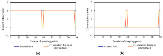
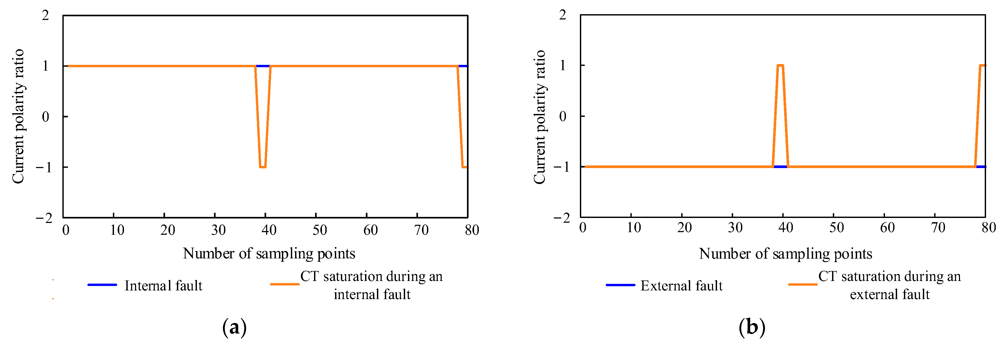
CT saturation can cause distortion in the secondary side output current waveform, making it unable to accurately reflect the magnitude and phase of the actual current on the primary side. Taking CT saturation caused by internal and external faults of a transformer as examples, the values under CT saturation and nonsaturation conditions are compared, as shown in Figure 2. Under internal fault conditions, is dominated by 1; under external fault conditions, is dominated by −1. The current polarity ratio effectively retains the positive and negative polarity characteristics, compensating for the loss of fault features caused by current distortion.
Figure 2.
(a) Current polarity ratio under internal fault conditions; (b) current polarity ratio under external fault conditions.
To make the time-domain current signal characteristics more significant under normal and fault conditions, the current polarity ratio and are defined. The historical sampling moments and the current sampling moment are accumulated to obtain :
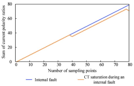
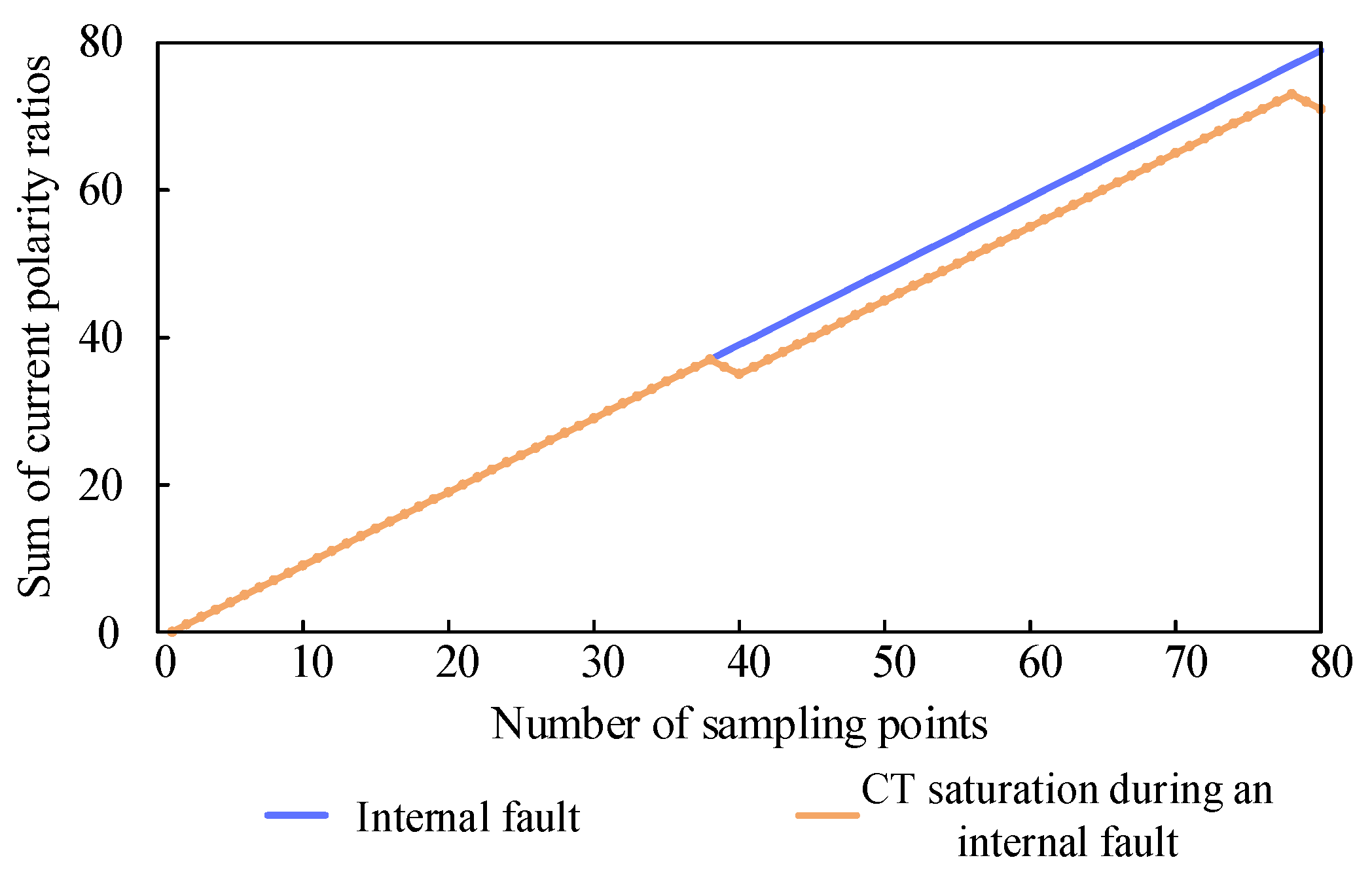
Taking an internal fault as an example, Figure 3 shows the of the phase A current. Both the nonsaturated and saturated conditions tend to increase in terms of the sum of the current polarity ratios.
Figure 3.
Changes in the sum of the current polarity ratios during CT saturation under internal faults.
2.2. Input Model of Time-Domain Characteristic Quantities for Transformers
The time-domain characteristic information from both sides of the transformer, including the three-phase voltage and current fault components, as well as the three-phase current polarity ratio defined in this paper and the sum of the three-phase current polarity ratios , is combined to form the input model of the transformer’s time-domain characteristic quantities. The fault components are calculated by taking the difference between the sampled values of three-phase electrical quantities within a specific data window and the corresponding sampled values from one cycle before fault occurrence. To demonstrate the effectiveness of the characteristic quantities constructed in this paper, the following three models are proposed:
Model 1: Composed of the three-phase voltage and current fault components from the high- and low-voltage sides of the transformer, including , totaling 12 sets of time-domain electrical characteristic quantities (corresponding to 12 channels), denoted as DM1.
Model 2: Combine the time-domain signals of Model 1 with the three-phase current polarity ratio , resulting in , totaling 15 sets of time-domain electrical characteristic quantities (corresponding to 15 channels), denoted as DM2.
Model 3: Combine the time-domain signals of Model 1 with the sum of the three-phase current polarity ratios , resulting in , totaling 15 sets of time-domain electrical characteristic quantities (corresponding to 15 channels), denoted as DM3.
2.3. Data Fusion Method
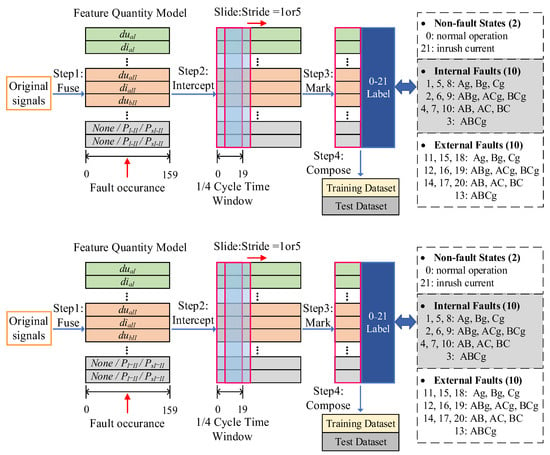
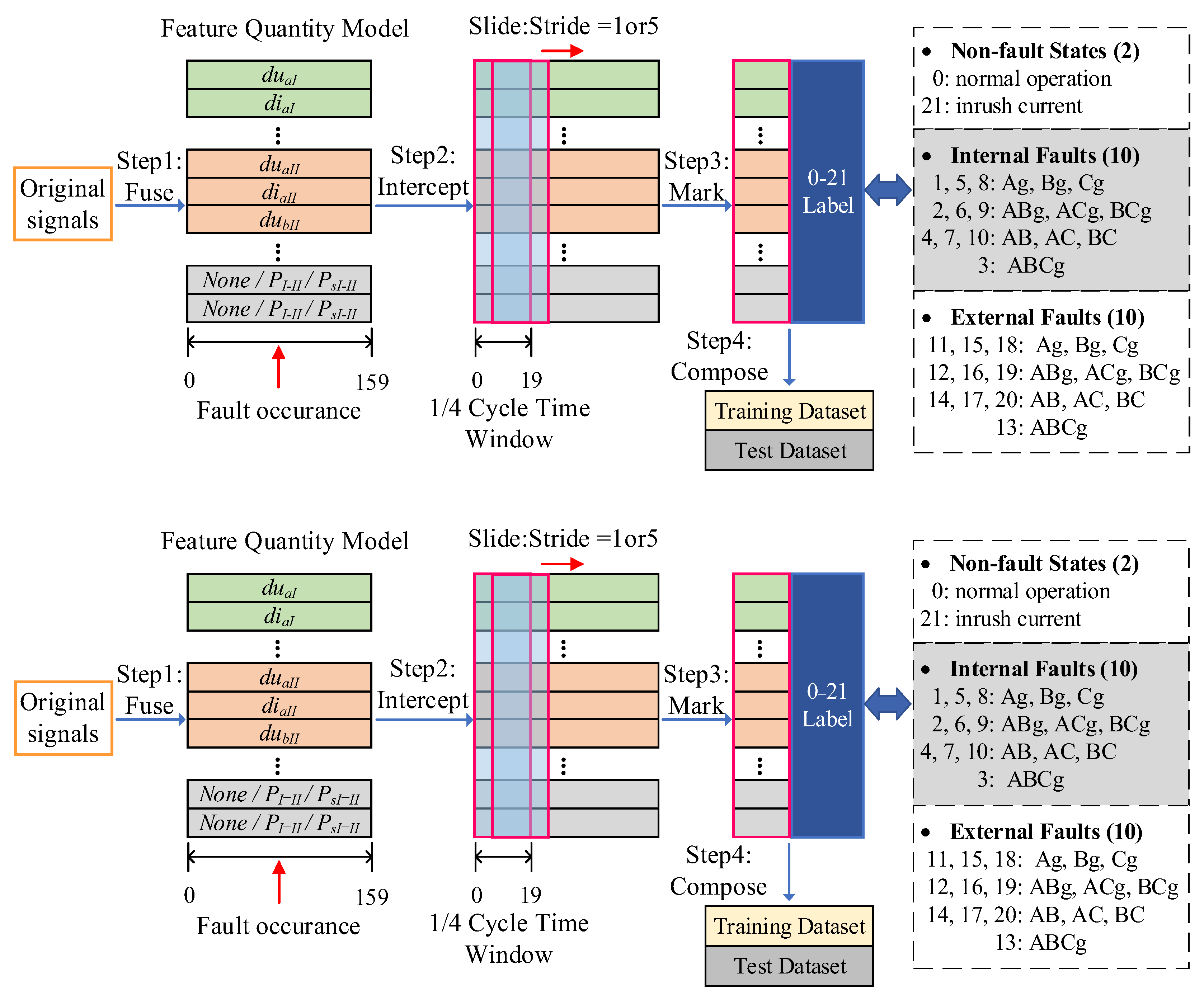
The time-domain signals need to undergo effective fusion to form the training and testing datasets. The data fusion processing flow is shown in Figure 4.
Figure 4.
Processing flowchart of data fusion and 22-class fault classification labeling.
When the time-domain feature quantity model is fused, the quantities of each channel are aligned in time stamps with data points as identifiers, thereby generating a sample set. Each channel covers data information from one cycle before and after fault occurrence. The power system frequency studied in this paper is 50 Hz. At the commonly used transformer sampling frequency of 4 kHz, one cycle contains 80 sampling points, while one sample comprises 160 sampling points, denoted as {0, 159}.
Subsequently, a sliding time window is employed to extract sample data with an equal step size starting from 0, thereby forming data segments for the training dataset. The length of the time window is set to 1/4 cycle, which corresponds to 20 sampling points at the 4 kHz sampling frequency. During the extraction of data segments for the training dataset, a sliding time window with a step size of 5 is adopted to enhance the speed of fault category discrimination by the model while preventing training overfitting. For instance, if the first extracted data segment is {0, 19}, the second extracted data segment is {5, 24}.
Similarly, a 1/4-cycle time window is applied. Starting from 0, the time window slides every step to extract sample data, forming the test dataset’s data segments. On the basis of the operational state information at the end time of each data segment, corresponding labeling is subsequently performed. The labeling method is illustrated in Figure 4. In this paper, 22 types of transformer operating states are set. Specifically, these correspond to 20 fault conditions, including single-phase-to-ground short circuits, phase-to-phase short circuits, two-phase-to-ground short circuits, and three-phase short circuits occurring both internally and externally to the transformer, as well as 2 nonfault conditions: normal operation and magnetizing inrush current.
3. Capsule Network Model Based on Channel Attention
3.1. Capsule Network
In traditional convolutional neural networks, positional information is lost when input vectors enter the pooling layer. The input model constructed in this paper consists of a combination of multichannel temporal electrical characteristic quantities, which inherently contain significant spatial structures. To effectively utilize and preserve the relative positional information between features, a capsule network is introduced to precisely capture the spatial correlations of various features in the equivalent image formed by the input vectors. Taking the phase change of the input signals as an example, the internal vectors of the capsule network adjust their values to accurately represent this new phase while keeping the vector length unchanged. The capsule network consists of a convolutional layer, a primary capsule layer, and a digit capsule layer.
(1) Primary Capsule Layer
The primary capsule layer normalizes the values of the output vector lengths between 0 and 1 using the squashing function, thereby representing the confidence of the capsules through their magnitudes. The formula for the squashing function is as follows:
where is the output vector of capsule j, is the input vector of capsule j, and represents the magnitude of vector .
(2) Digit Capsule Layer
The digit capsule layer incorporates a dynamic routing algorithm, which iteratively optimizes the connection weights between primary capsules and digit capsules. Its core lies in updating weights on the basis of the directional alignment between the prediction vectors of lower-level capsules and the output vectors of higher-level capsules. The iterative formula is as follows:
Here, is the prediction capsule, is the weight matrix, is the output vector of the i-th primary capsule, reflects the connection between the prediction vector and the output vector, with an initial value of 0, is the output vector of the j-th digit capsule, and is the coupling coefficient used to evaluate the importance of lower-level capsules to higher-level capsules.
(3) Loss Function
The capsule network adopts the margin loss function as the optimization objective, calculates the loss values for each category and accumulates them to obtain the overall loss value. The formula is as follows:
Here, represents the magnitude of the output vector from the k-th class capsule. serves as a label indicator variable, which is 1 when the sample belongs to the k-th class and 0 otherwise. defines the minimum value for the magnitude of the output vector of correctly classified capsules, typically set to 0.9. defines the maximum value for the magnitude of the output vector of incorrectly classified capsules, typically set to 0.1. represents the weight coefficient for the lower-bound loss, balancing the proportion of classification loss between positive and negative samples, typically set to 0.5.
3.2. Capsule Network Based on a Channel Attention Mechanism
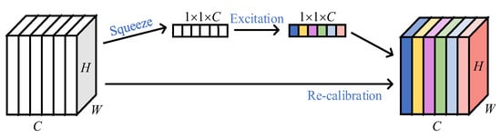
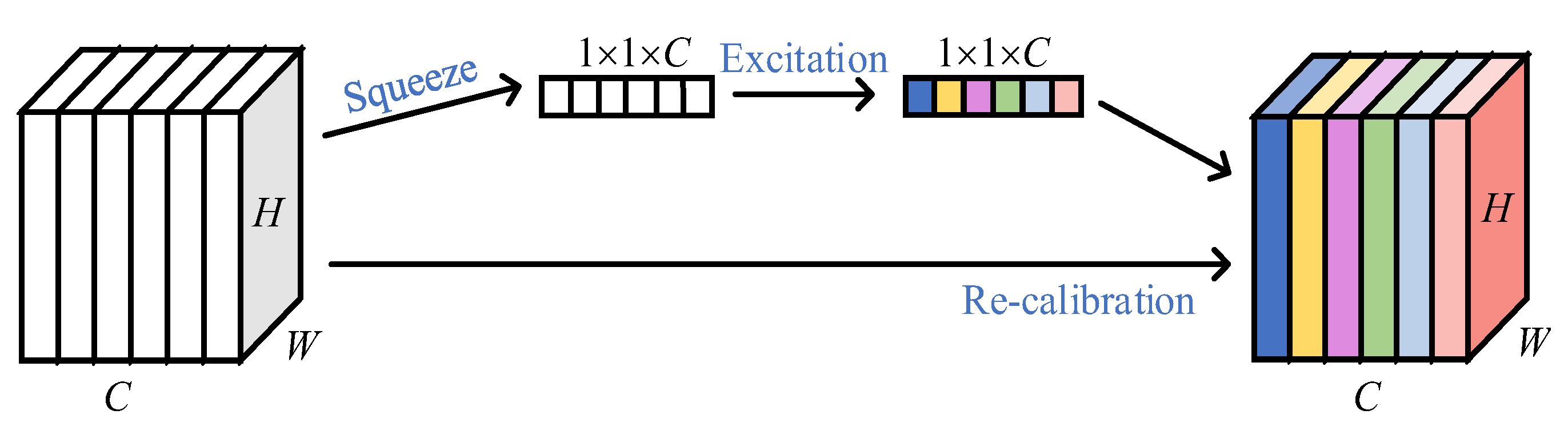
To enable the network to balance the weights of different channels, this paper introduces the squeeze-and-excitation block (SE block), whose processing flow is shown in Figure 5. Here, represents the shape and size of the input feature map F, and denote the height and width of the feature map, respectively, and indicates the number of channels.
Figure 5.
SE channel attention mechanism.
In the squeeze stage, the feature map F is compressed into a one-dimensional vector via global average pooling, followed by nonlinear transformation through a fully connected layer to learn the dependencies between channels and generate corresponding weight coefficients for each channel. Finally, in the recalibration stage, the channel weights are multiplied channelwise with the feature map F, ensuring that the output dimensions remain . Through this approach, the network enhances the feature responses of important channels while suppressing information from less critical channels, thereby improving the model’s expressive power and discriminative performance.
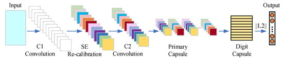
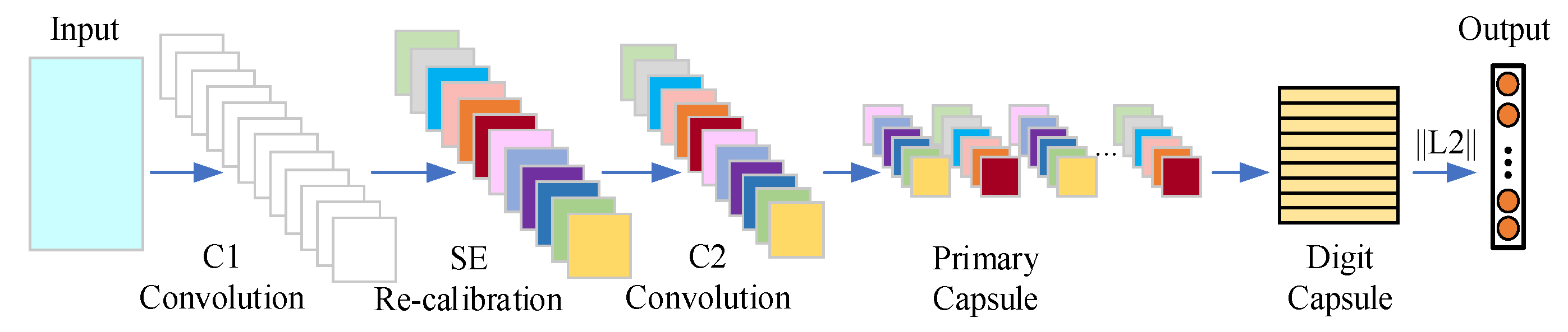
On this basis, in this paper, a channel attention-based capsule network, SE-CapsuleNet, is constructed on top of a convolutional neural network, whose structure is illustrated in Figure 6.
Figure 6.
SE-Capsule network.
Convolutional layer C1 contains 28 convolutional kernels for preliminary feature extraction. The features subsequently pass through the SE module to balance the weights of each channel. The processed features are then fed into the convolutional layer C2, which employs 28 convolutional kernels for deep feature extraction.
The capsule network consists of 20 convolutional kernels. Afterward, the two-dimensional feature maps output by the convolutional layer are flattened into one-dimensional vectors through the primary capsule layer. These vectors are grouped into sets of 18 and concatenated into high-dimensional vectors, forming the digit capsules. The digit capsule layer uses a dynamic routing algorithm for three iterative operations, ultimately outputting several vectors. The number of these vectors corresponds to the total number of categories in the classification task, i.e., the number of operating conditions of the transformer. The magnitude of each vector represents the predicted probability of the corresponding category. The dimensional transformations during the forward propagation of SE-CapsuleNet are shown in Table 2.
Table 2.
Dimension transformation during SE-CapsuleNet forward propagation.
4. SE-CapsuleNet-Based Transformer Operational State Discrimination
4.1. Transformer Simulation Dataset
A transformer model, as shown in Figure 1, is built on the PSCAD platform, with a system frequency of 50 Hz and a sampling frequency of 4 kHz. The rated capacity of transformer T1 is 200 MVA, with a voltage ratio of 220/110 kV, and it adopts a Y/Y connection. Line Line1 has a total length of 60 km, with a resistance of 0.025 Ω/km and an inductance of 0.379 Ω/km.
For the transformer shown in Figure 1, after the protection elements S1 and S2 are disconnected, when S1 is closed, the transformer generates an inrush current when no load is close to the system. Three-phase voltage and current time-domain data from protection elements S1 and S2 of the transformer are collected to form sample data. The sample data under fault conditions include data from one cycle before and after the fault, i.e., 160 sampling points; the sample data under inrush current conditions include data from ten cycles after closing, i.e., 800 sampling points.
The simulation parameters for the training and testing datasets are shown in Table 3. Here, the initial power angle is defined as the phase difference between Source1 and Source2, which can be adjusted by modifying the phase angle value of Source1. The fault distance is defined as the distance from the fault point to protection unit S1 of Line1. In this paper, the fault occurrence time is set at 0.2 s.
Table 3.
Simulation parameter settings of the dual-winding transformer.
The training set is partitioned into training, testing, and validation subsets in a ratio of 7:2:1. These subsets are utilized for model construction and fine-tuning during the training phase. The test set is obtained using parameter combinations and sliding windows that are completely different from those of the training set, which facilitates independent testing of the model under a broader range of operating conditions.
4.2. Training and Testing Results
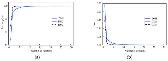
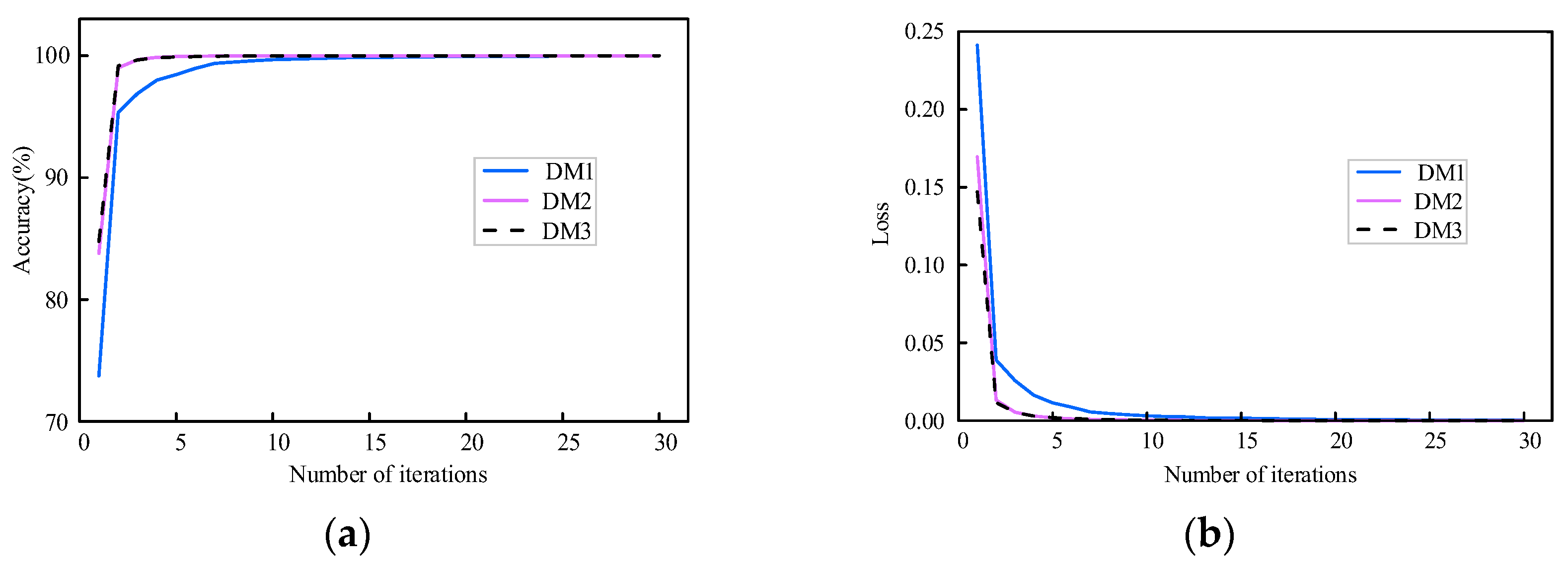
After the time-domain features are input into models DM1–DM3 to complete the fusion processing operation, they are fed into the SE-CapsuleNet network for training. The performance changes in models DM1–DM3 during the training period are shown in Figure 7. Expected convergence is exhibited by the network during iterative optimization, evidenced by increasing recognition accuracy and decreasing loss values, consistent with typical deep learning training patterns.
Figure 7.
(a) Recognition accuracy versus iteration number; (b) loss versus iteration number.
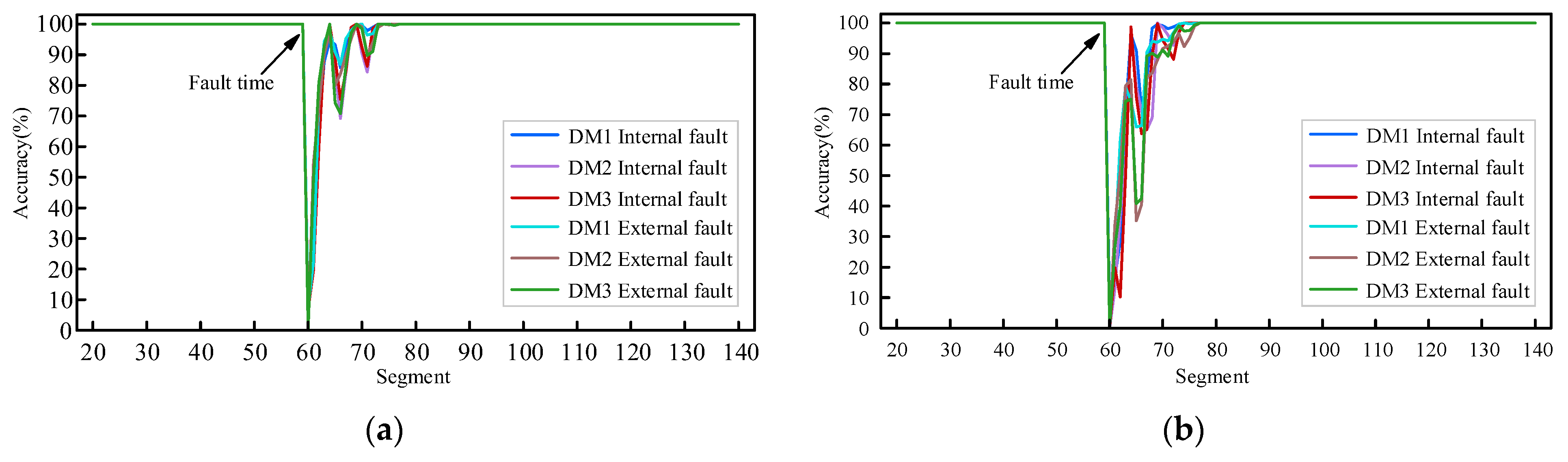
When the test set in Table 3 is used for online performance verification, when the time window is set to 1/4 cycle, the 60th data segment first captures fault information. The changes in the identification accuracy of models DM1–DM3 for internal and external faults of the transformer are shown in Figure 8. During normal system operation, all the models demonstrate good state recognition capabilities. Starting from the 60th data segment, the identification accuracy of each model significantly decreases. However, identification accuracy is recovered as the proportion of fault characteristics within data segments increases.
Figure 8.
(a) Discrimination for high-elevation faults; (b) discrimination for low-elevation faults.
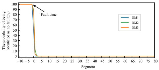
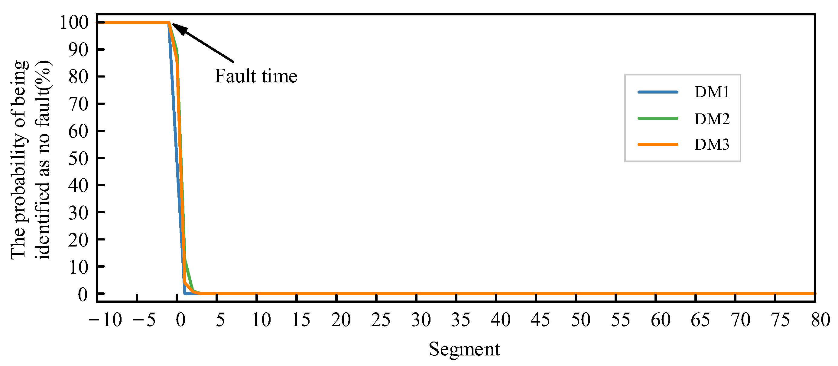
The probabilities of models DM1–DM3 still misjudging abnormal states as normal states after a fault occurs are shown in Figure 9. The results indicate that, at the latest within 3 sampling points after the fault, the faulty state is no longer misclassified as a nonfault type.
Figure 9.
Probability of each model incorrectly classifying a fault as normal.
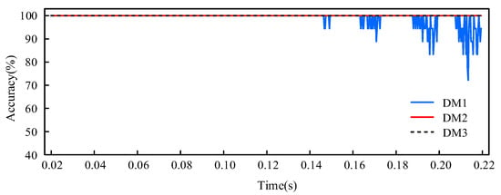
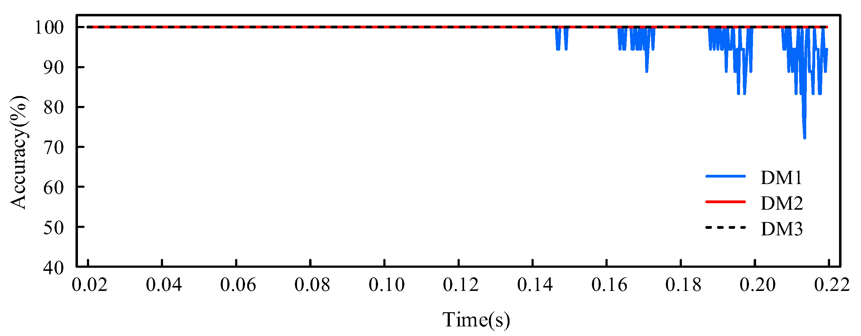
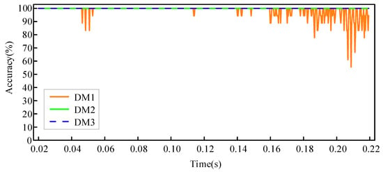
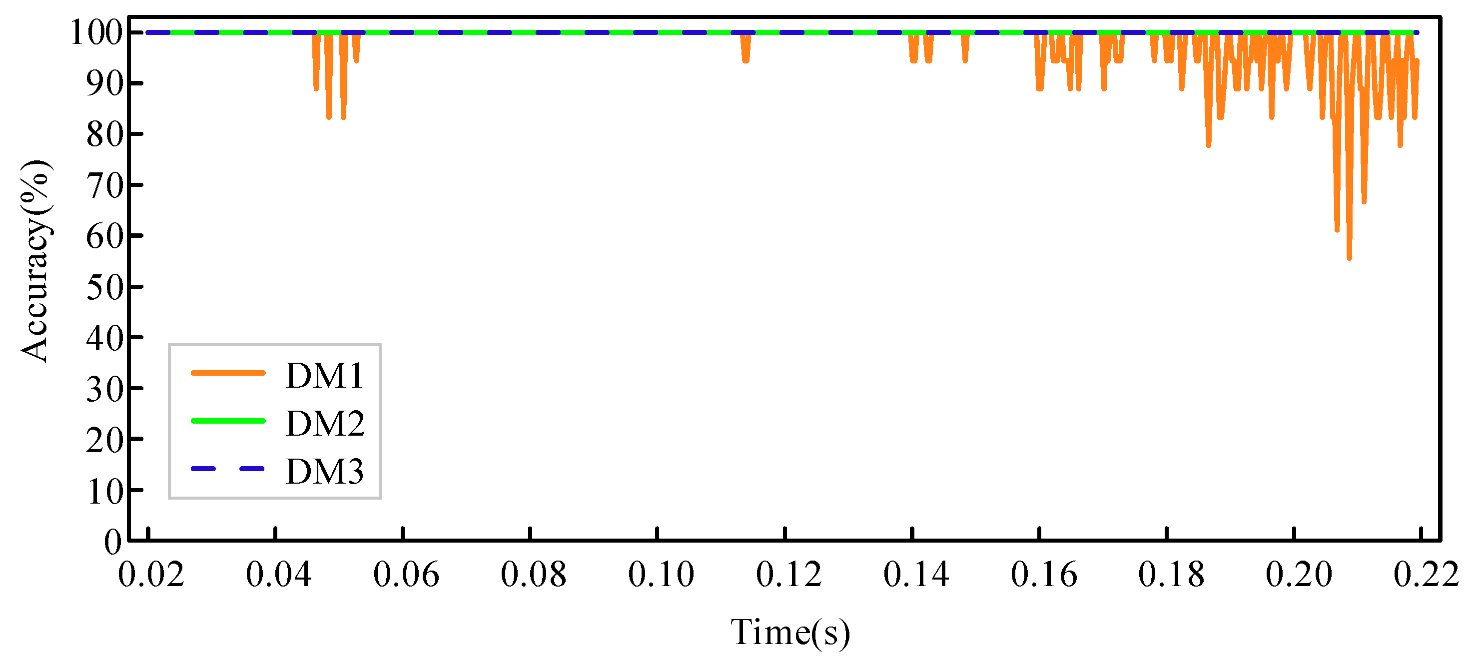
The performance of models DM1–DM3 in identifying the transformer inrush current is shown in Figure 10. At the 0.02 s mark, a transformer no-load closing condition is set to generate an inrush current. The results show that DM1 has the risk of misidentifying the inrush current state as an internal transformer fault starting from the 6th cycle, whereas DM2 and DM3 maintain accurate identification throughout the ten cycles after the closing operation.
Figure 10.
Recognition accuracy of each model for the excitation inrush current condition.
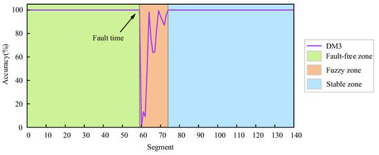
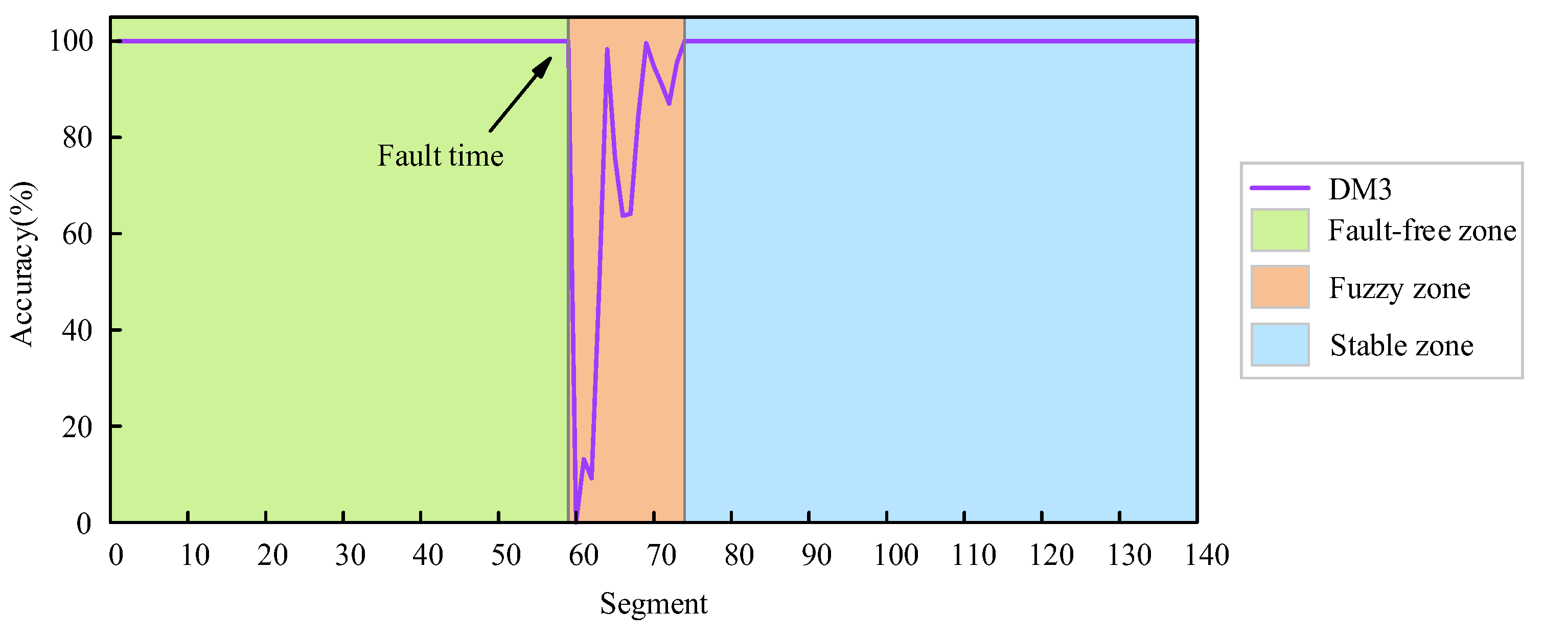
On the basis of the performance of each model at different stages, their operation processes can be divided into three parts: the fault-free zone, the fuzzy zone, and the stable zone. Taking DM3 as an example, a specific illustration is shown in Figure 11. The boundary between the fault-free zone and the fuzzy zone is the time node at which the model first misidentifies an abnormal state as a normal state. The dividing line between the fuzzy zone and the stable zone is defined as the time node when the recognition accuracy reaches 100% again or when the fluctuation amplitude stabilizes.
Figure 11.
Performance phase partitioning of model DM3.
Additionally, this paper evaluates the actual effectiveness of the proposed SE-CapsuleNet model by constructing two deep learning models: the SECNN and the CAP. The SECNN model replaces the capsule network part of the SE-CapsuleNet model with two convolutional layers, two max-pooling layers, one fully connected layer, and one softmax layer. The CAP model is obtained by removing the SE block layer from the SE-CapsuleNet model. Performance validation was conducted using the test samples from Table 3. The results are presented in Table 4. It can be observed from the data in Table 4 that the proposed SE-CapsuleNet achieves the highest overall average accuracy and F1 score, and the duration of the fuzzy zone is the shortest. The overall online performance is the best among the three, which strongly verifies the superiority of the SE-CapsuleNet proposed in this paper in highlighting fault features and learning capabilities. Subsequent studies will systematically explore the performance of the SE-CapsuleNet model under different operating conditions, such as CT saturation, inrush current, and high-resistance grounding faults.
Table 4.
Comparative analysis of accuracy, ambiguous zone, and F1 score for various models.
5. Analysis of Factors Influencing Model Performance
(1) CT Saturation Caused by Faults
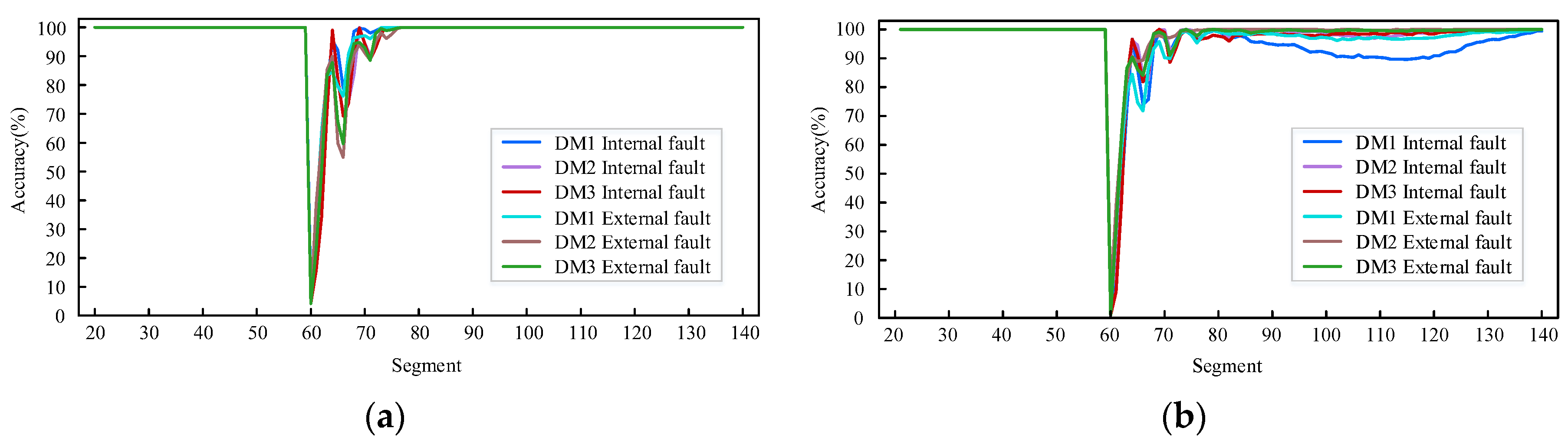
In this study, a dataset containing CT saturation characteristics is constructed by adjusting the current transformer ratio parameters in the original test dataset. The model validation results for this dataset are shown in Figure 12a,b. The test results indicate that compared with the model without CT saturation samples, the model trained with CT saturation samples has shorter durations in the fuzzy region and maintains 100% fault discrimination accuracy in the stable region.
Figure 12.
(a) Model accuracy with CT saturation samples in the training set; (b) model accuracy without CT saturation samples in the training set.
Additionally, within a certain period after the fault occurs, the accuracy rates of various models exhibit a specific trend of change: first decreasing, then increasing, followed by another decline, and then increasing again. To understand this phenomenon, the relationship between current distortion under CT saturation and the variation in model accuracy rates was further investigated.
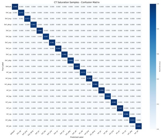
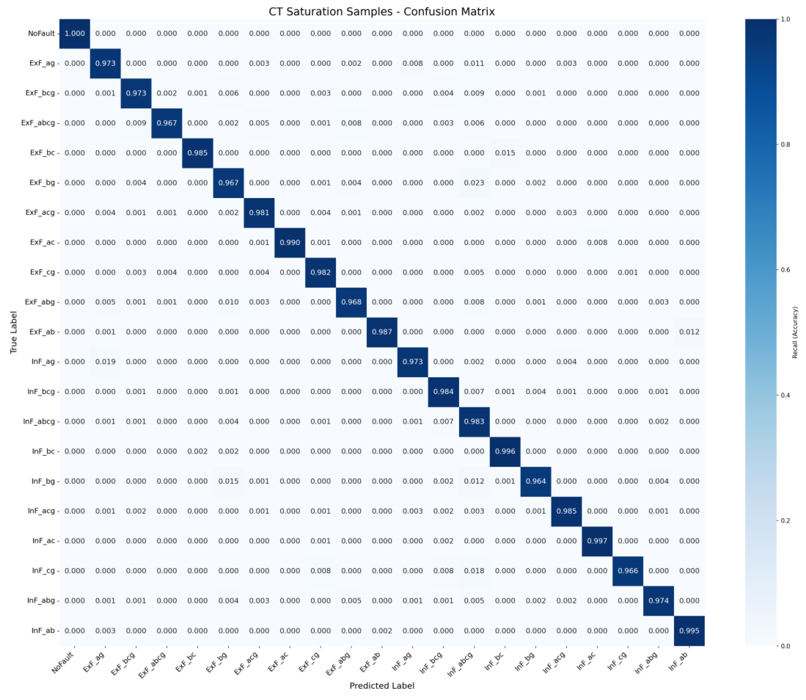
Figure 13 presents the confusion matrix obtained by testing exclusively with samples involving CT saturation from the test set. It can be observed that the identification accuracy for various types of internal and external faults generally exceeds 96%. A small number of misclassifications are primarily concentrated among fault types with similar features; however, severe misjudgments crossing the internal/external boundary do not occur. This indicates that the model remains capable of accurately delineating the protection zone and correctly classifying faults under conditions of CT saturation.
Figure 13.
Confusion matrix of the CT saturation scenario.
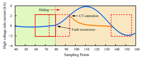
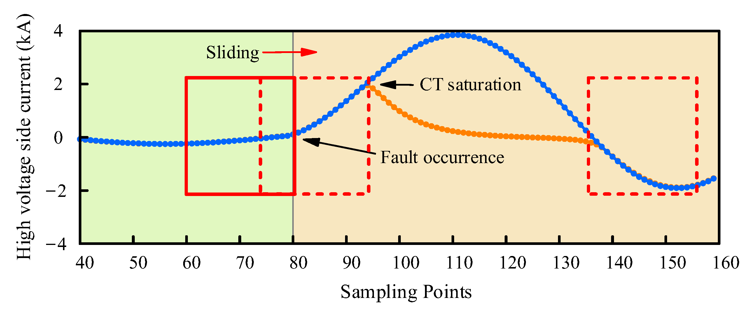
The dynamic changes in current waveforms under high-voltage-side CT saturation conditions are shown in Figure 14. During the initial 3 ms after the fault is triggered, the current transformer can still maintain linear transmission characteristics, and the normal current signals captured within the sampling window remain undistorted. As time progresses, distorted current data gradually begin to mix into the sampling window, with its proportion continuously increasing. The narrower the time window is, the greater the relative proportion of distorted data; when the time window fully covers the saturated CT data, the sampled signals are completely dominated by distorted waveforms, leading to a sharp decline in recognition accuracy. As the time window subsequently shifts, the proportion of distorted signals within the window starts to decrease, and the model’s accuracy rate recovers accordingly.
Figure 14.
High-voltage-side current waveform.
(2) Inrush Current Containing Residual Magnetism
The generation and development of the inrush current are constrained by two key parameters: the closing phase angle and the residual magnetic flux in the core. Among these, the closing phase angle determines the waveform characteristics of the inrush current, whereas the residual magnetic flux determines its peak magnitude and the angle of interruption. When residual magnetic flux exists in the core, the peak value of the inrush current generated at the instant of transformer energization significantly exceeds that under zero residual flux conditions. On the basis of the nonlinear magnetic flux-current characteristic curve of the transformer, this paper employs the superposition of a DC component in the PSCAD simulation environment to equivalently simulate the residual magnetic effect. In the simulation, the residual magnetic parameter is set to 0.7 p.u., thereby forming a test dataset for the closing inrush current that includes residual magnetic factors. The test results are shown in Figure 15.
Figure 15.
Variation in accuracy of models DM1-DM3 under remanence conditions.
As shown in Figure 15, model DM1 exhibits numerous identification errors within the first 10 cycles, which are primarily concentrated after the 6th cycle, with significant fluctuations in accuracy. In contrast, model DM3 achieves the best accuracy throughout all 10 cycles.
(3) Single-phase High-resistance Grounding Fault
To verify the identification capabilities of each model in high-impedance fault scenarios, in this paper, the fault resistance parameters are adjusted to three levels—260 Ω, 350 Ω, and 400 Ω—based on the original dataset, thereby constructing simulation conditions for minor faults inside and outside the transformer protection zone.
Testing revealed that in the nonfault zone and stable zone, the average accuracy of the three models under the three fault resistance levels essentially remained at 100%, whereas the average performance in the fuzzy zone is shown in Table 5. The duration of the fuzzy region for all three models is less than 5 ms, indicating that the proposed deep learning method in this paper can identify single-phase grounding faults with fault resistances as high as 400 Ω, reliably achieving accurate discrimination of minor faults inside and outside the protection zone.
Table 5.
Performance of models DM1–DM3 under single-phase high-impedance faults.
(4) Noise Interference
In this paper, three intensity levels of Gaussian white noise were superimposed on the original test samples, with the signal-to-noise ratio parameters set to 20 dB, 30 dB, and 40 dB. The experimental results show that the correct recognition rates of the DM1–DM3 algorithms for normal operating conditions are all 100%, with little difference in performance between the fuzzy and stable regions.
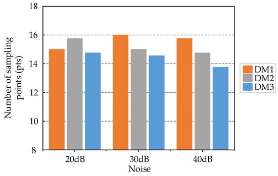
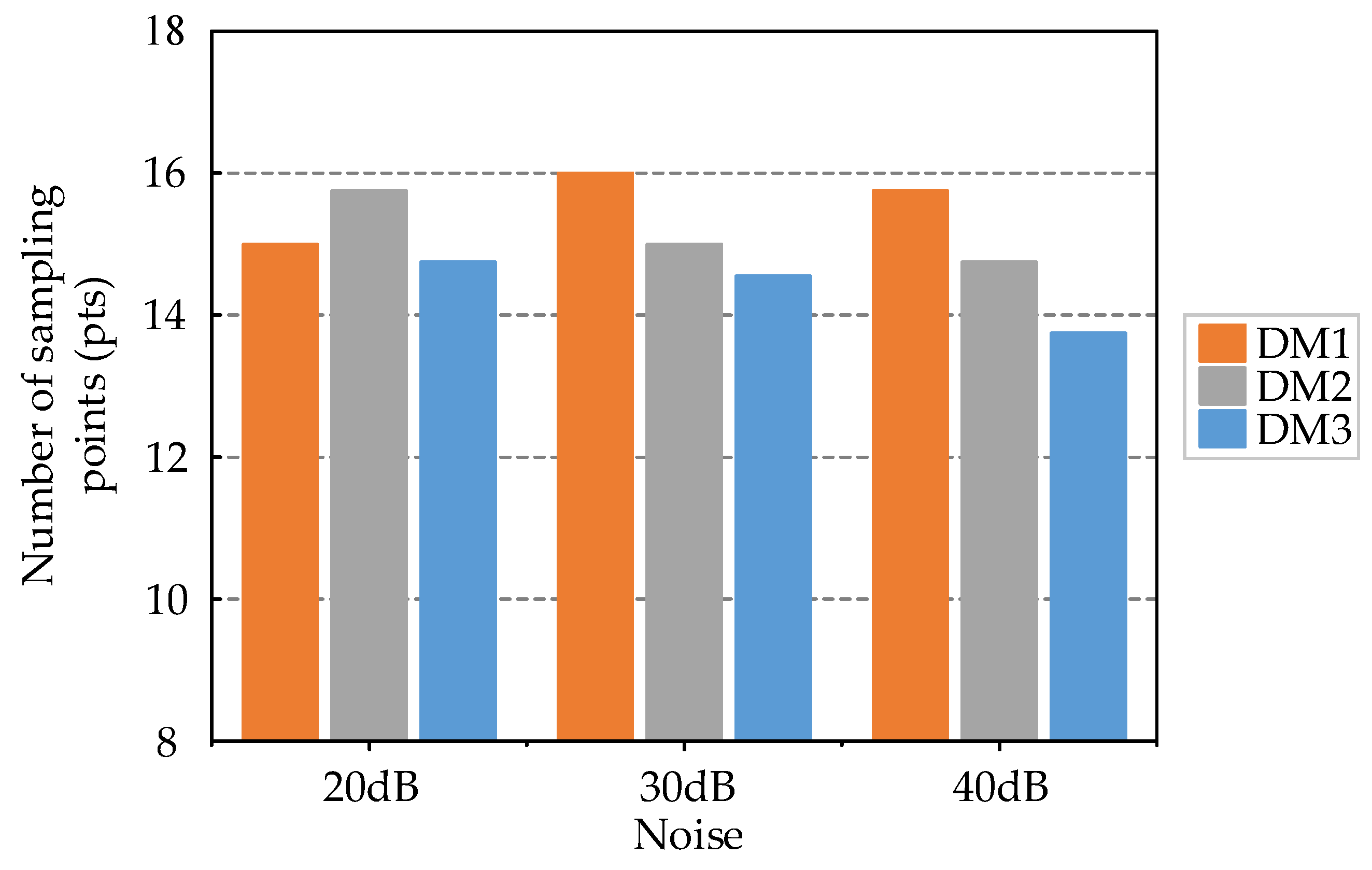
The number of sampling points occupied by fuzzy regions in each model is shown in Figure 16. Models DM1 to DM3 were not trained with noisy samples but still exhibited strong robustness. A comparison of the time spans of the recognition fuzzy regions among the three models reveals that the differences are small, and all the time spans are controlled within the selected time window length. In the stable region, the three models can still correctly identify all test samples, demonstrating good antinoise performance and effectively handling 20 dB noise interference environments.
Figure 16.
The number of sampling points occupied by fuzzy regions under different noises in each model.
(5) Different Short-Circuit Capacities and Voltage Levels
The input features selected in this paper primarily consider the following points:
- (1)
- The fault component is calculated by differentiating the post-fault electrical quantities from the pre-fault ones, thereby eliminating the steady-state component. The resulting transient feature waveforms possess similar morphological characteristics across transformers of different voltage levels;
- (2)
- As defined in Equation (1), the current polarity characteristic takes values only from {−1, 0, 1}, representing the polarity relationship between the currents on both sides of the transformer. This polarity-based feature is independent of voltage levels or topological structures and depends solely on the fault location;
- (3)
- The sum of the current polarity characteristics represents the trend of polarity variation over time, which is similarly independent of voltage levels or topological structures.
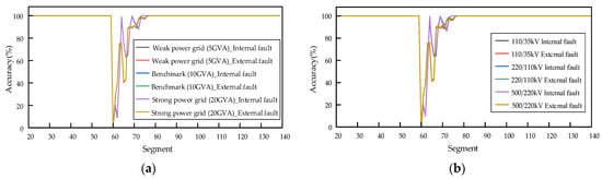
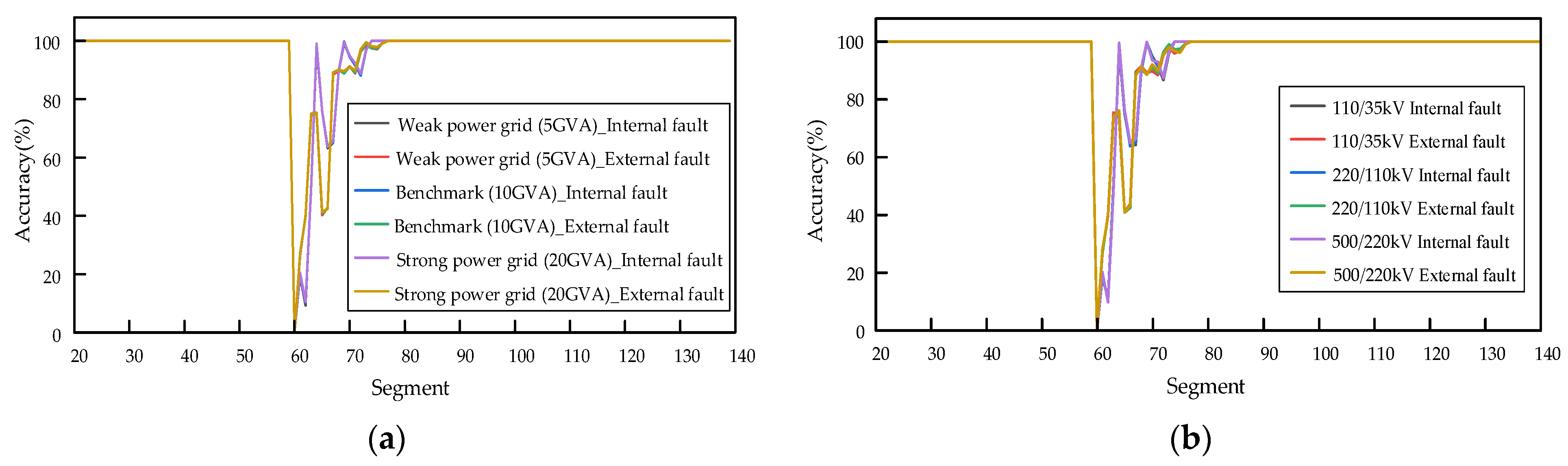
In this study, a new test set is constructed by altering the short-circuit capacity and voltage level based on the original test set to evaluate the model. The test results are shown in Figure 17:
Figure 17.
(a) Model accuracy under different short-circuit capacities; (b) model accuracy under different voltage levels.
It can be observed from the test results that the differences in accuracy and fuzzy zone duration under different conditions are insignificant. This indicates that variations in system short-circuit capacity have a negligible impact on model performance. Furthermore, by adjusting the normalization constant, the model can adapt to different voltage levels, confirming that features such as polarity and fault components are independent of voltage levels.
6. New Transformer Relay Protection Scheme
The SE-CapsuleNet proposed in this paper can effectively distinguish between normal transformer operation, internal/external faults, and inrush current phenomena without the need for additional activation criteria. Given that model DM3 demonstrates the best comprehensive performance, it is selected as the model for the protection scheme.
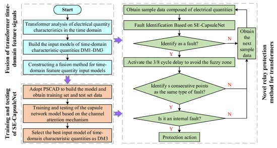
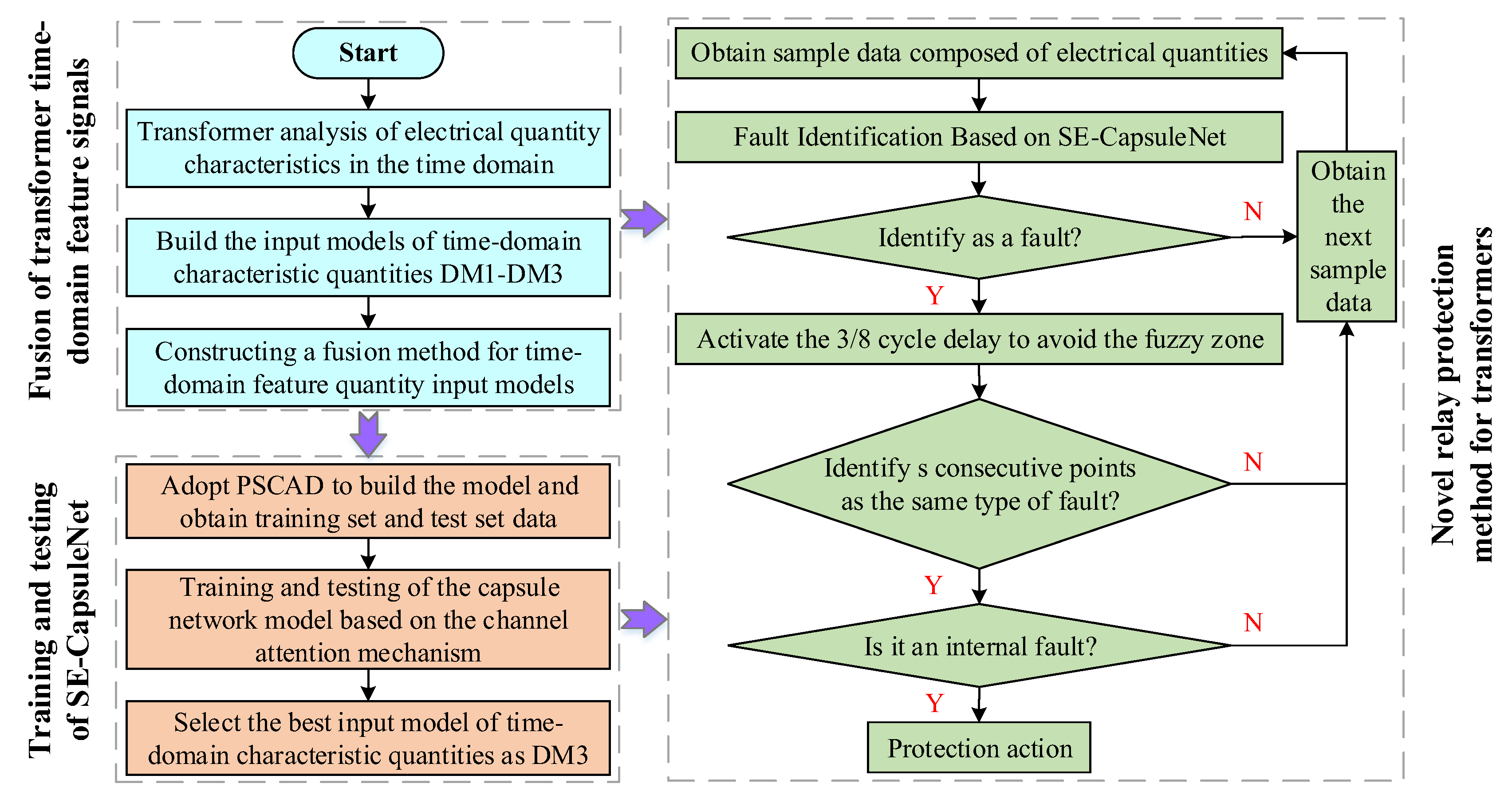
To effectively eliminate interference from ambiguous identification zones and reduce the likelihood of protection device maloperation, it is necessary to introduce an appropriate safety margin. Experimental verification reveals that when the safety margin is set to 1/8 cycle (with a 1/4 cycle time window for sample data capture), the total superimposed duration is 3/8 cycles. This parameter configuration successfully avoids misjudgment risks in ambiguous zones.
Furthermore, to enhance protection security, this paper adopts a multipoint continuous confirmation mechanism instead of directly outputting results based on single-sampling-point judgments. The core concept involves setting continuous detection windows with a length of s data points. A trip command is issued only when s consecutive data points confirm the same internal fault type. The value of s can be adjusted according to actual protection requirements. Practical applications demonstrate that setting s to 10 sampling points ensures sufficient safety in protection operations. In a 4 kHz sampling environment, one cycle corresponds to 80 sampling points. Furthermore, the test dataset in this paper is obtained by extracting sample data using a time window with a step size of one sampling point; therefore, 10 sampling points correspond to 1/8 cycle.
A flow chart of the novel protection scheme proposed in this paper is illustrated in Figure 18. When the parameter s is determined to be 10, the specific implementation steps of the proposed SE-CapsuleNet model for transformer relay protection are as follows: When the model first detects a fault signal, regardless of whether it belongs to an internal or external fault category, a 7.5 ms delay is triggered to avoid interference from ambiguous regions. During this delay period, the model does not output any discrimination information. After the delay ends, the model resumes its discrimination output. At this point, if the discrimination results of 10 consecutive sampling points are completely consistent and all point to a specific internal fault type, it is confirmed that the transformer has experienced that type of internal fault, and the tripping procedure is initiated to disconnect all sides of the transformer. Additionally, the protection does not operate in scenarios such as inconsistent discrimination results across 10 consecutive points or when 10 consecutive points are identified as external faults. The pseudo-code for the flowchart is provided in Appendix B to describe the protection scheme more clearly.
Figure 18.
Flow chart of the protection plan.
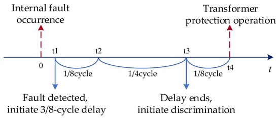
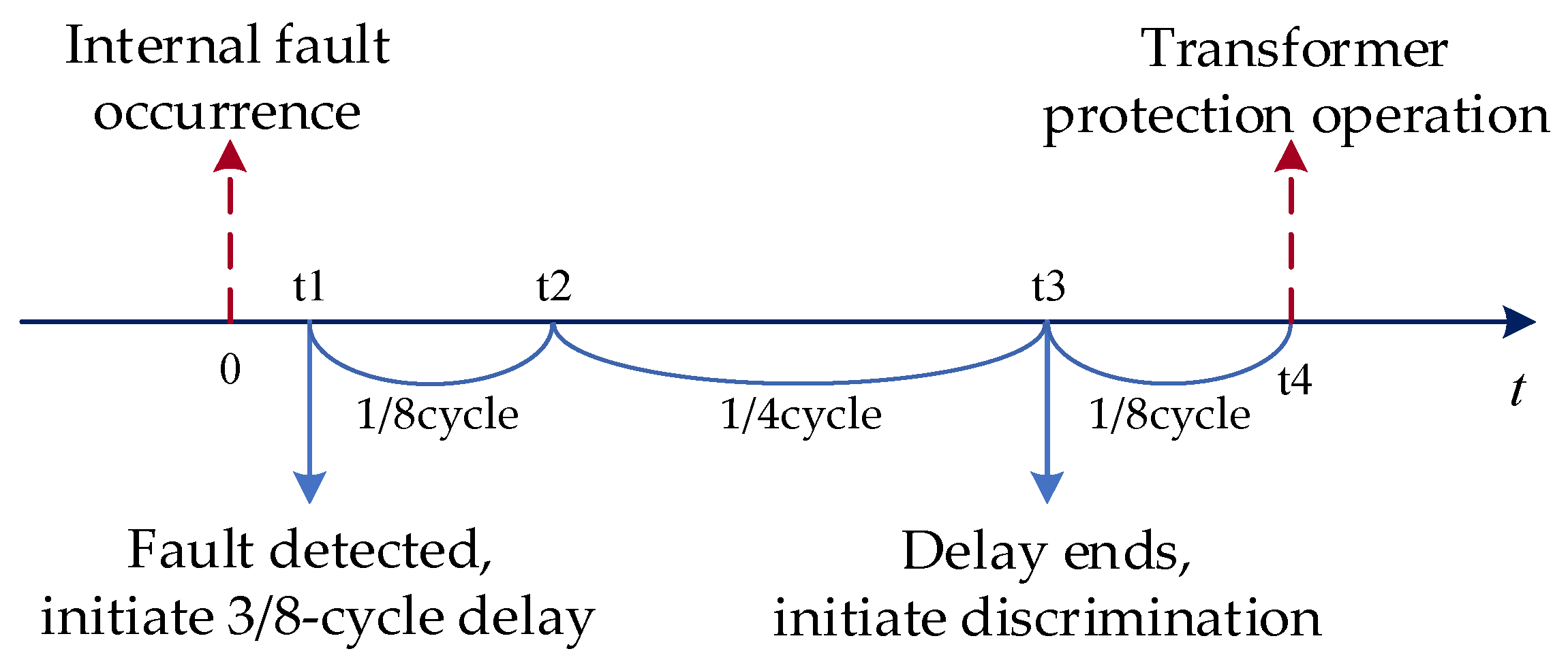
The timing sequence is illustrated in Figure 19. Upon an internal fault occurrence at time 0, the fault is detected by the SE-CapsuleNet at t1, initiating a 3/8-cycle delay. Data sampling resumes at t2 following a 1/8-cycle safety margin. Given the 1/4-cycle time window, the discrimination result is re-evaluated 1/4 cycle after t2. Transformer protection is actuated at t4 when 10 consecutive points are identified as the same internal fault type. Consequently, the total operating time, comprising t1, the 3/8-cycle delay (consisting of the safety margin and time window), and the 1/8 cycle for point verification, is maintained within 12 ms.
Figure 19.
Timing diagram of the new transformer relay protection scheme.
The proposed relay protection scheme in this paper eliminates the need for complex settings and offers a more flexible configuration. It effectively avoids inrush current and CT saturation without the need for additional discrimination conditions. When facing single-phase high-resistance grounding faults, it can withstand fault resistances up to 400 Ω. Even in a 20 dB noise environment, it maintains rapid and accurate fault discrimination capabilities, fully demonstrating excellent anti-interference characteristics and system stability. Furthermore, as the time-domain features adopted in this paper can all be calculated from three-phase electrical quantities, and the sampling frequency is consistent with that commonly used in transformer protection, the relay protection method proposed in this paper does not require additional sensors compared to traditional transformer protection, thereby demonstrating superior economic efficiency.
7. Summary
Transformer protection faces challenges in inrush, CT saturation, and high-resistance faults. A time-domain model utilizing voltage-current components and polarity ratios is constructed, and an SE-CapsuleNet is employed for classification. Validation is performed via PSCAD simulations. Key findings are as follows:
- (1)
- Polarity ratios are incorporated for input integration. While misjudgments occur in voltage-current-only models (DM1) after the 6th cycle, a fairly high accuracy is maintained by the proposed model (DM3) within 10 cycles. This is sufficient for fault type classification in the steady state.
- (2)
- The fuzzy zone is reduced to 4 ms by SE-CapsuleNet, outperforming SECNN (5 ms) and CAP (4.5 ms). Furthermore, in the stable zone, each type of working condition is given a very high confidence coefficient, such as nearly 100%. This validates the architecture’s efficiency.
- (3)
- Clear working condition classifications are sustained under adverse conditions (CT saturation, 0.7 p.u. remanence, 400 Ω fault resistance, 20 dB noise). Fuzzy zones for high-resistance faults are limited to 5 ms.
- (4)
- A scheme utilizing a 3/8 cycle delay and 10-point confirmation is proposed. Identification is completed within 12 ms at 4 kHz, eliminating manual threshold dependence.
The limitations of this study are hereby acknowledged. First, retraining is required for distinct topologies. Second, renewable energy characteristics (e.g., weak infeed) are not addressed; future work is directed towards relevant feature incorporation. Finally, as this study is simulation-based, hardware-in-the-loop (HIL) verification and complexity quantification remain to be performed.
Author Contributions
Conceptualization, H.S.; methodology, H.Y., X.C., R.L., S.X. and R.H.; software, J.Z.; validation, J.Z.; formal analysis, R.H.; investigation, R.H.; resources, H.S.; data curation, H.Y. and R.L.; writing—original draft preparation, X.C. and R.L.; writing—review and editing, J.Z.; visualization, S.X.; supervision, H.S.; project administration, H.S.; funding acquisition, H.S. All authors have read and agreed to the published version of the manuscript.
Funding
This research was funded by Yunnan Power Grid Co., Ltd. Science and Technology Project Funding, grant number YNKJXM20240221.
Data Availability Statement
The original contributions presented in this study are included in the article.
Conflicts of Interest
Authors Hengchu Shi, Hao You, Xiaofan Chen and Shoudong Xu were employed by the company Yunnan Power Grid Co., Ltd., China. The remaining authors declare that the research was conducted in the absence of any commercial or financial relationships that could be construed as a potential conflict of interest.
Appendix A
A simulation circuit diagram of PSCAD is illustrated in Figure A1. Signals I1 and V1 are measured on the high-voltage side, while I2 and V2 are measured on the low-voltage side, with fault resistance controlled by signal Ron. Simulation parameters are detailed in Table A1. Additionally, the Type JA current transformer model is utilized, with parameter settings listed in Table A2.
Figure A1.
PSCAD model.
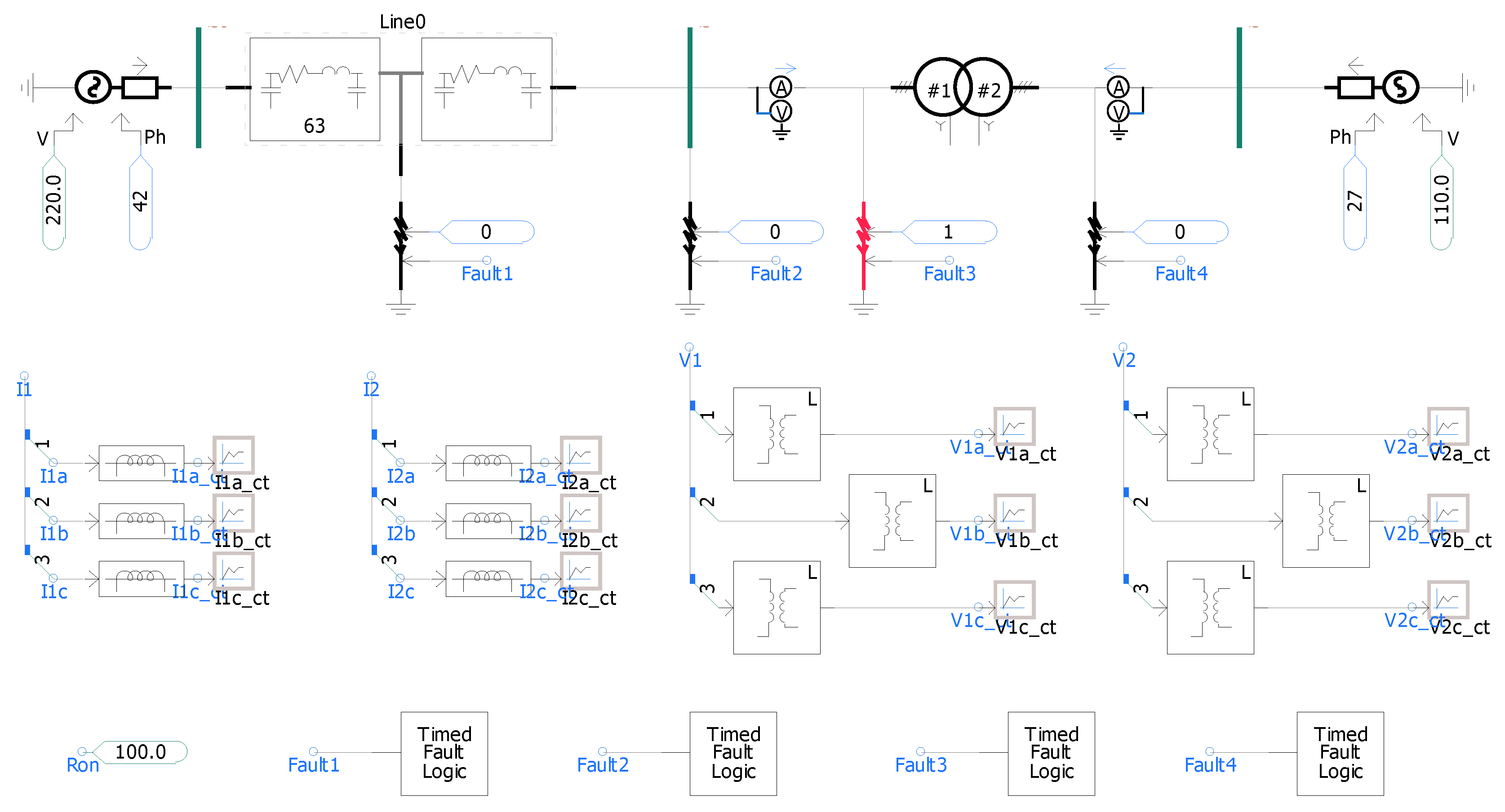
Table A1.
System parameter table.
Table A2.
Current transformer parameter table.
Appendix B
| Algorithm A1: Novel Transformer Relay Protection Scheme Based on SE-CapsuleNet |
| Input: Transformer voltage/current signals (time-domain samples) Output: Protection trip command or Continue monitoring Constants: cycle (Safety margin delay) (Consecutive confirmation threshold ) kHz (Sample rate) |
| 1: Procedure MAIN() 2: Initialize , 3: Initialize , 4: While protection is enabled do 5: 6: 7: If then 8: 9: If not then 10: 11: , , 12: Continue 13: End If 14: 15: If then 16: Continue 17: End If 18: If then 19: 20: Else 21: , 22: End If 23: If and then 24: 25: Return 26: End If 27: Else 28: , , 29: End If 30: End While 31: End Procedure |
References
- Medeiros, R.P.; Costa, F.B. A wavelet-based transformer differential protection with differential current transformer saturation and cross-country fault detection. IEEE Trans. Power Deliv. 2017, 33, 789–799. [Google Scholar] [CrossRef] [Scilit]
- Shahbazi, N.; Bagheri, S.; Gharehpetian, G.B. Transformer differential protection scheme based on self-adaptive biased characteristic curve and considering cross-country faults. Int. J. Circuit Theory Appl. 2023, 51, 1110–1131. [Google Scholar] [CrossRef] [Scilit]
- Liu, Q.; Mei, N.; Wang, Z.; Sun, J.; Zhou, S. Enhanced Transformer Overcurrent Protection via Oil Temperature Acceleration. Energies 2024, 17, 4916. [Google Scholar] [CrossRef] [Scilit]
- Porawagamage, G.; Dharmapala, K.; Chaves, J.S.; Villegas, D.; Rajapakse, A. A review of machine learning applications in power system protection and emergency control: Opportunities, challenges, and future directions. Front. Smart Grids 2024, 3, 1371153. [Google Scholar] [CrossRef] [Scilit]
- Key, S.; Ko, C.-S.; Song, K.-J.; Nam, S.-R. Fast Detection of Current Transformer Saturation Using Stacked Denoising Autoencoders. Energies 2023, 16, 1528. [Google Scholar] [CrossRef] [Scilit]
- Ghanbari, T.; Samet, H.; Ghafourifard, J. New approach to improve sensitivity of differential and restricted earth fault protections for industrial transformers. IET Gener. Transm. Distrib. 2016, 10, 1486–1494. [Google Scholar] [CrossRef] [Scilit]
- Chen, Z.; Li, H.; Dong, X.; He, Y.; Zhou, Q.; Zhang, Y.; Zhang, Y. Magnetizing inrush current elimination strategy based on a parallel type asynchronous closing hybrid transformer. IEEE Trans. Power Electron. 2022, 38, 931–943. [Google Scholar] [CrossRef] [Scilit]
- Peres, L.M.; Silva, K.M. Power transformer protection using an instantaneous-current-value negative sequence differential element. Int. J. Electr. Power Energy Syst. 2019, 105, 96–106. [Google Scholar] [CrossRef] [Scilit]
- Oliveira, M.O.; Bretas, A.S.; Ferreira, G.D. Adaptive differential protection of three-phase power transformers based on transient signal analysis. Int. J. Electr. Power Energy Syst. 2014, 57, 366–374. [Google Scholar] [CrossRef] [Scilit]
- Gunda, S.K.; Dhanikonda, V.S.S.S.S. Discrimination of transformer inrush currents and internal fault currents using extended kalman filter algorithm (Ekf). Energies 2021, 14, 6020. [Google Scholar] [CrossRef] [Scilit]
- Shahbazi, N.; Bagheri, S.; Gharehpetian, G.B. Performance improvement of transformer differential protection during cross-country fault using hyperbolic S-transform. IEEE Trans. Instrum. Meas. 2022, 71, 1–9. [Google Scholar] [CrossRef] [Scilit]
- Zhao, Y.C.; Crossley, P. Countermeasure to prevent the incorrect blocking of differential protection applied to converter transformers. IEEE Trans. Power Deliv. 2020, 35, 95–105. [Google Scholar] [CrossRef] [Scilit]
- Jazebi, S.; Doğan, R.; Kovan, B.; De Leon, F. Reduction of inrush currents in toroidal transformers by sector winding design. IEEE Trans. Power Electron. 2016, 31, 6776–6780. [Google Scholar] [CrossRef] [Scilit]
- Łukaniszyn, M.; Baron, B.; Kolańska-Płuska, J.; Majka, Ł. Inrush current reduction strategy for a three-phase dy transformer based on pre-magnetization of the columns and controlled switching. Energies 2023, 16, 5238. [Google Scholar] [CrossRef] [Scilit]
- Samantaray, S.R. Phase-space-based fault detection in distance relaying. IEEE Trans. Power Deliv. 2011, 26, 33–41. [Google Scholar] [CrossRef] [Scilit]
- Hajipour, E.; Vakilian, M.; Sanaye-Pasand, M. Current-transformer saturation compensation for transformer differential relays. IEEE Trans. Power Deliv. 2015, 30, 2293–2302. [Google Scholar] [CrossRef] [Scilit]
- Shah, A.M.; Bhalja, B.R.; Patel, R.M.; Bhalja, H.; Agarwal, P.; Makwana, Y.M.; Malik, O.P. Quartile based differential protection of power transformer. IEEE Trans. Power Deliv. 2020, 35, 2447–2458. [Google Scholar] [CrossRef] [Scilit]
- Zacharias, D.; Gokaraju, R. Prototype of a negative-sequence turn-to-turn fault detection scheme for transformers. IEEE Trans. Power Deliv. 2015, 31, 122–129. [Google Scholar] [CrossRef] [Scilit]
- Bakhshipour, M.; Namdari, F.; Rezaeealam, B.; Sedaghat, M. Setting-Less Differential Protection of Power Transformers Based on Wavelet Transform. Iran. J. Sci. Technol. Trans. Electr. Eng. 2024, 48, 1685–1695. [Google Scholar] [CrossRef] [Scilit]
- Balaga, H.; Gupta, N.; Vishwakarma, D.N. GA trained parallel hidden layered ANN based differential protection of three phase power transformer. Int. J. Electr. Power Energy Syst. 2015, 67, 286–297. [Google Scholar] [CrossRef] [Scilit]
- Afrasiabi, S.; Afrasiabi, M.; Parang, B.; Mohammadi, M. Integration of accelerated deep neural network into power transformer differential protection. IEEE Trans. Ind. Inform. 2019, 16, 865–887·. [Google Scholar] [CrossRef] [Scilit]
- Afrasiabi, S.; Afrasiabi, M.; Parang, B.; Mohammadi, M. Designing a composite deep learning based differential protection scheme of power transformers. Appl. Soft Comput. 2020, 87, 105975. [Google Scholar] [CrossRef] [Scilit]
- Afsharisefat, R.; Jannati, M.; Shams, M. A power transformer differential protection method based on variational mode decomposition and CNN-BiLSTM techniques. IET Gener. Transm. Distrib. 2024, 18, 767–778. [Google Scholar] [CrossRef] [Scilit]
- Wang, L.; Zhao, X.; Pei, J.; Tang, G. Transformer fault diagnosis using continuous sparse autoencoder. SpringerPlus 2016, 5, 448. [Google Scholar] [CrossRef] [Scilit]
- Cao, H.; Zhou, C.; Meng, Y.; Shen, J.; Xie, X. Advancement in transformer fault diagnosis technology. Front. Energy Res. 2024, 12, 1437614. [Google Scholar] [CrossRef] [Scilit]
- Dalian, Y.; Junjun, Z.; Hui, L. Capsule networks for intelligent fault diagnosis: A roadmap of recent advancements and challenges. Expert Syst. Appl. 2025, 296, 128814. [Google Scholar] [CrossRef] [Scilit]
- Sevov, L.; Khan, U.; Zhang, Z. Enhancing power transformer differential protection to improve security and dependability. IEEE Trans. Ind. Appl. 2017, 53, 2642–2649. [Google Scholar] [CrossRef] [Scilit]
- Mishra, M.; Singh, J.G. A comprehensive review on deep learning techniques in power system protection: Trends, challenges, applications and future directions. Results Eng. 2025, 25, 103884. [Google Scholar] [CrossRef] [Scilit]



Disclaimer/Publisher’s Note: The statements, opinions and data contained in all publications are solely those of the individual author(s) and contributor(s) and not of MDPI and/or the editor(s). MDPI and/or the editor(s) disclaim responsibility for any injury to people or property resulting from any ideas, methods, instructions or products referred to in the content. |
© 2026 by the authors. Licensee MDPI, Basel, Switzerland. This article is an open access article distributed under the terms and conditions of the Creative Commons Attribution (CC BY) license.