Mechanism Analysis of MMC Oscillation Based on Damping Path Decomposition

Abstract

In modern power systems with a high penetration of power-electronic-interfaced resources, grid-following (GFL) Modular Multilevel Converters (MMCs) face a risk of sub-synchronous oscillations caused by the coupling of multiple control loops. Such oscillations are driven by converter control, with damping jointly shaped by dynamic coupling among the phase-locked loop (PLL), DC voltage control (DVC), reactive power control (RPC), and other inner loops. Conventional impedance-based analysis cannot trace such oscillations back to specific control loops, nor can it characterize their interaction. To address this gap, this paper establishes a small-signal model of the GFL MMC and characterizes its second-order DC voltage control (DVC) loop by analogy with the rotor motion equation of a synchronous machine, thereby enabling an analysis of how the other control loops affect the damping of the DVC. Based on this model, a damping path decomposition method is proposed to quantitatively decompose the system electrical damping into four contributions: the intrinsic effect of the DVC, the influence of the PLL on the DVC, the influence of the RPC on the DVC, and the effect arising from the interaction between the PLL and RPC. Analysis results indicate that the DVC itself possesses a certain degree of positive damping, RPC provides positive damping, while the PLL and its interaction with RPC contribute negative damping to the DVC loop. The influence of control parameters and operating conditions on the overall system damping is then investigated. The predicted trends are confirmed through EMT simulation, providing a theoretical basis for parameter tuning and stable MMC operation under weak-grid conditions.

1. Introduction

Modern power systems are undergoing a profound transition driven by the large-scale integration of renewable energy and power-electronic-interfaced equipment. Owing to its high degree of modularity, high-quality output waveforms, and independently controllable active and reactive power, MMC-based flexible HVDC transmission has become key equipment for large-scale renewable energy delivery and long-distance transmission. In large-capacity DC infeed scenarios such as the West-to-East Power Transmission Project, the equivalent strength of the receiving-end AC system is continuously weakened as the share of conventional synchronous generation declines. As a result, the dynamic characteristics of the MMC increasingly dominate the small-signal stability of the receiving-end system [1]. Against this background, revealing the mechanism by which the MMC’s own control and operating point affect system stability is critical for the safe and stable operation of new power systems.

In recent years, numerous practical engineering cases and simulation studies have reported wideband oscillation phenomena dominated by converters, with frequencies ranging from a few Hz to several tens of Hz. Sub-synchronous oscillations from a few Hz up to just below power frequency are particularly prominent [1,2]. For an MMC using GFL control, complex dynamic coupling exists between outer loops such as the PLL, DC voltage control (DVC), and reactive power control (RPC), and inner loops such as the current loop and circulating current suppression control. Once control parameters or operating conditions change, the system’s damping in this frequency band may drop significantly or even become negative, triggering sustained oscillation [2,3]. An urgent scientific challenge therefore remains: to quantitatively characterize how each control loop and its interactions contribute to damping, and to explain the mechanism underlying such oscillations.

Regarding the small-signal stability of converter-dominated systems, existing research falls mainly into three categories of methods: impedance-based analysis, eigenvalue analysis, and damping torque analysis. The impedance method starts from port characteristics and determines system stability via the generalized Nyquist criterion. It has been widely used in wideband oscillation analysis of converters. For example, to account for the effects of PLL bandwidth and SCR [4], and in impedance modeling that considers positive- and negative-sequence frequency coupling [5]. However, the impedance method is essentially a “black-box” port description, making it difficult to trace the cause of instability back to specific control loops or to characterize the interaction between different control loops. Eigenvalue analysis provides modes and participation factors, but it offers little physical insight into the underlying oscillation mechanism. In contrast, damping torque analysis originated from sub-synchronous oscillation research on synchronous machines. It decomposes electrical torque into synchronizing and damping components, has clear physical meaning, and facilitates identification of the sources of negative damping [6].

To introduce the concept of damping torque into converter analysis, reference [7] points out that the DC capacitor voltage dynamics of a grid-following converter share the same form as the rotor equation of motion of a synchronous machine, with the DC capacitor acting as an equivalent inertial element. This makes it possible to extend the damping torque analysis of synchronous machines to converters, and the resulting methods has been further applied to reduced-order transient stability and singular perturbation analysis [7,8,9]. However, studies show that the classical damping torque analysis does not strictly hold for converters. References [10,11] therefore defined a corrected synchronizing coefficient and damping coefficient. Furthermore, existing studies have separately studied the damping effects of the inner loops of grid-forming converters [12] and the outer loops of grid-connected converters [13], laying the groundwork for quantitative analysis of the damping contribution of control loops.

To separate damping contributions of multiple control loops, the Path Analysis Method (PAM) combines transfer-function block diagrams with damping torque analysis. The method decomposes system damping into several parallel “paths,” each quantifying the contribution of a different dynamic channel. This method has been applied to direct-drive wind farms delivered via flexible DC transmission [14], sub-synchronous interaction analysis of renewable energy delivered via LCC-HVDC [15], and sub-synchronous control interaction analysis induced by the PLL in multi-converter systems [16]. These applications demonstrate its advantage in identifying the negative-damping contribution of loops such as the PLL and terminal voltage control [17]. However, PAM has not yet been applied to MMC, let alone extended to characterize the interactions among its internal control loops. Moreover, most existing path-decomposition studies neglect the fast time scale, commonly treating the current inner loop as an instantaneous element and omitting it from the decomposition entirely [18,19]. A quantitative, mechanism-level characterization of the contribution of individual control loops and their coupling to system damping remains absent from the existing literature.

To address the above gaps, this paper investigates the sub-synchronous oscillation mechanism of the MMC. Based on the developed model, damping path decomposition is employed to reveal the contributions of different control loops to damping. The main work and contributions are as follows. (1) A small-signal model of the grid-following MMC is established and verified through detailed EMT simulation. (2) A damping path decomposition method is proposed based on damping torque analysis, which quantitatively decomposes the system’s electrical damping into contributions from four paths: the intrinsic effect of the DVC, the influence of the PLL on the DVC, the influence of the RPC on the DVC, and the effect arising from the interaction between the PLL and RPC. The analysis shows that the path where the PLL acts alone, together with its interaction path with reactive power control, is the main source of negative damping. (3) This paper systematically studies the influence of control parameters (the PLL, reactive power control, and the current inner loop) and operating points (grid strength and active/reactive power output) on the damping contributions analytically predicted by the proposed path decomposition method. The predicted overall trends are confirmed through time-domain EMT simulation. This provides a theoretical basis for parameter tuning and stable MMC operation under weak-grid conditions and complex operating scenarios. The time-domain EMT simulations validate the predicted response of the system, confirming that the small-signal model and the proposed decomposition method accurately capture the stability trends.

The remainder of this paper is organized as follows. Section 2 establishes the small-signal model of the single-MMC system, verifies its correctness, and defines the damping of the second-order DC voltage loop by analogy with the second-order equation of motion of rotor dynamics. Section 3 proposes the damping path decomposition method, quantifies the damping of each path, and analyzes the sub-synchronous oscillation mechanism. Section 4 studies the influence of control parameters and operating points on damping. Section 5 concludes the paper.

2. System Description and Modeling

2.1. MMC Control Structure

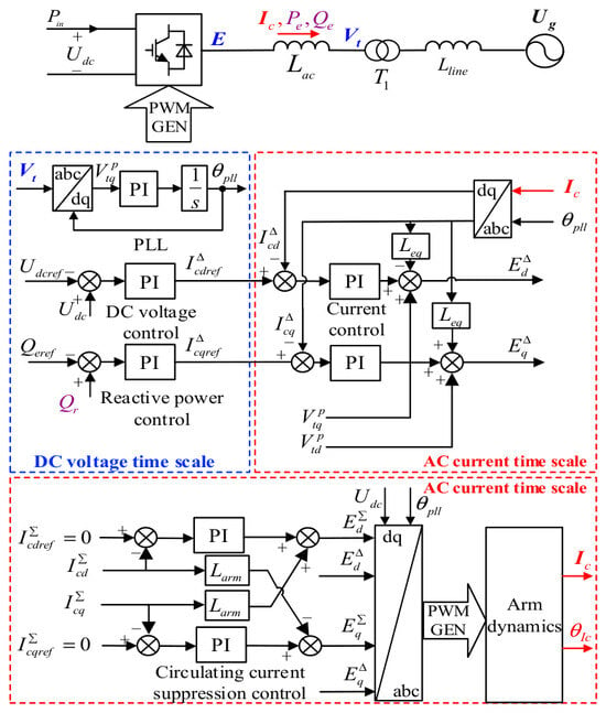
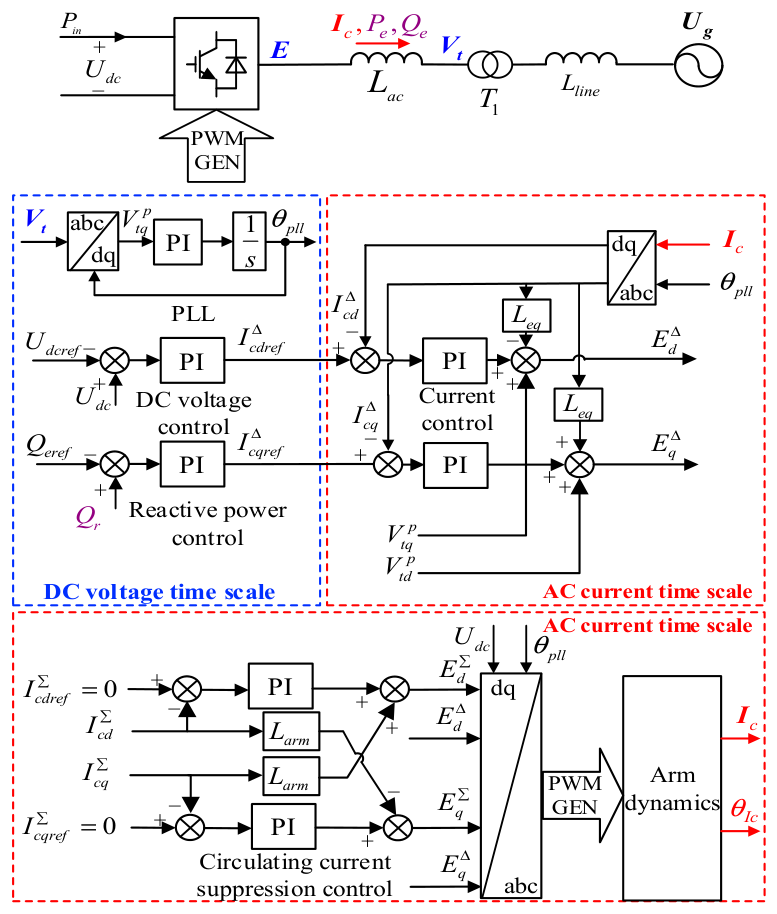
This paper studies the MMC receiving-end system, considering the sending-end input as constant power. As shown in the typical control block diagram of the grid-following MMC system in Figure 1, the outer-loop control of the MMC includes the PLL, DC voltage control, and reactive power control. Among these, the PLL tracks the phase of the terminal voltage, thereby providing a phase reference for all other controls of the MMC. The DC voltage control yields the inner-loop d-axis current reference, thereby maintaining DC voltage stability. Reactive power control has a similar structure. The inner-loop control of the MMC includes current control and circulating current suppression control. An additional circulating current suppression controller can reduce losses and improve the output waveform. The outer-loop controller calculates the inner-loop current reference from the DC voltage and reactive power command values. The inner-loop current control then regulates the converter output voltage so that the dq-axis current increment ΔI_cd/ΔI_cq rapidly tracks this reference, improving power quality and providing fast, accurate current protection. Meanwhile, the differential-mode and common-mode voltages generated by the inner loop are modulated to dynamically produce the internal current.

Figure 1. Typical control block diagram of the MMC.

Since this paper focuses on the oscillation mode in the subsynchronous frequency band, which lies well below the frequency of the retained second-harmonic dynamics, the small-signal model retains harmonic components up to the second order [20]. Harmonic components of higher order (sixth and above) typically have much smaller amplitude in the MMC’s arm current and submodule capacitor voltage than the fundamental and second-harmonic components, and their contribution to the system dynamics is correspondingly small. Neglecting these higher-order harmonics therefore has negligible impact on the analysis of the subsynchronous oscillation mechanism addressed in this paper.

2.2. Small-Signal Model of the MMC and Its Verification

The following modeling conventions and simplifying assumptions are adopted in the model derivation. The terminal voltage and PLL-related quantities are expressed in per-unit values normalized to the rated AC voltage and nominal system frequency, and the PLL is linearized around its steady-state operating point, where the terminal-voltage phase is aligned with the d-axis. The line and arm resistances listed in Table A1 are retained throughout the derivation. The following simplifying assumptions are then introduced: (i) the PWM switching delay is neglected, as its phase contribution is negligible within the sub-synchronous frequency range considered; (ii) the AC grid is assumed balanced, with unbalanced conditions and asymmetrical faults excluded from the present analysis; and (iii) the sending-end input power is assumed constant, such that the sending-end converter and DC-network dynamics are not modeled separately.

2.2.1. Linearized Model of Control Loops

The output θ_pll of the PLL is:

$${\theta }_{\mathit{pll}}=V_{\mathit{tq}}^p(k_{\mathit{ppll}}+{\displaystyle \frac{k_{\mathit{ipll}}}{s}}){\displaystyle \frac{1}{s}}$$

(1)

Linearizing Equation (1) gives:

$$\Delta {\theta }_{\mathit{pll}}=\underset{G_{\mathit{pll}}(s)}{\underbrace{(k_{\mathit{ppll}}+{\displaystyle \frac{k_{\mathit{ipll}}}{s}}){\displaystyle \frac{1}{s}}}}\Delta V_{\mathit{tq}}^p$$

(2)

The d- and q-axis components of the terminal voltage rotating vector V_t in the PLL reference frame are, respectively:

$$\left\{\begin{array}{c}\begin{array}{l}{\theta }_{\mathit{err}}={\theta }_{\mathit{Vt}}-{\theta }_{\mathit{pll}}\\ V_{\mathit{td}}^p=V_t\cos {\theta }_{\mathit{err}}\end{array}\\ V_{\mathit{tq}}^p=V_t\sin {\theta }_{\mathit{err}}\end{array}\right.$$

(3)

Noting that the PLL error θ_err is zero in steady state, linearizing Equation (3) gives:

$$\left\{\begin{array}{l}\Delta V_{\mathit{td}}^p=\Delta V_t\hfill \\ \Delta V_{\mathit{tq}}^p=V_{t0}\Delta {\theta }_{\mathit{err}}\hfill \end{array}\right.$$

(4)

The relationship between the d- and q-axis components of the internal current rotating vector I_c in the PLL reference frame and its magnitude I_c and phase ${\theta }_{Ic}^p$ in that frame is:

$$\left\{\begin{array}{c}{I}_c=\sqrt{I_{\mathit{cd}}^2+I_{\mathit{cq}}^2}\\ {\theta }_{\mathit{Ic}}^p=\arctan ({\displaystyle \frac{I_{\mathit{cq}}^p}{I_{\mathit{cd}}^p}})\end{array}\right.$$

(5)

The power factor angle of the MMC is:

φ_c = θ_Vt − θ_Ic

(6)

Since the PLL phase equals the terminal voltage phase in steady state, we have:

$${\phi }_{c0}={\theta }_{\mathit{Vt}0}-{\theta }_{\mathit{Ic}0}=-{\theta }_{\mathit{Ic}0}^p$$

(7)

Therefore, linearizing Equation (5) and substituting Equation (7) gives:

$$\left\{\begin{array}{c}\Delta I_c=\cos {\phi }_{c0}\Delta I_{\mathit{cd}}^p-\sin {\phi }_{c0}\Delta I_{\mathit{cq}}^p\\ \Delta {\theta }_{\mathit{Ic}}^p={\displaystyle \frac{\sin {\phi }_{c0}}{I_{c0}}}\Delta I_{\mathit{cd}}^p+{\displaystyle \frac{\cos {\phi }_{c0}}{I_{c0}}}\Delta I_{\mathit{cq}}^p\end{array}\right.$$

(8)

The active power output by the MMC is:

$$P_e=V_{\mathit{td}}^p{I}_{\mathit{cd}}^p+V_{\mathit{tq}}^p{I}_{\mathit{cq}}^p$$

(9)

Linearizing Equation (9) and substituting it into Equation (4) gives:

$$\begin{array}{ll}\Delta P_e& =V_{\mathit{td}0}^p\Delta I_{\mathit{cd}}^p+V_{\mathit{tq}0}^p\Delta I_{\mathit{cq}}^p+I_{\mathit{cd}0}^p\Delta V_{\mathit{td}}^p+I_{\mathit{cq}0}^p\Delta V_{\mathit{tq}}^p\\ & =\underset{\Delta P_{e1}}{\underbrace{V_{t0}\Delta I_{\mathit{cd}}^p}}+\underset{\Delta P_{e2}}{\underbrace{I_{c0}\cos {\phi }_{c0}\Delta V_t-V_{t0}{I}_{c0}\sin {\phi }_{c0}\Delta {\theta }_{\mathit{err}}}}\end{array}$$

(10)

Equation (10) shows that the active power increment consists of two parts: the part caused by changes in the DC voltage control output (ΔP_e1), and the part caused by external disturbances (ΔP_e2).

The DC capacitor dynamics can be described as:

$$P_{\mathit{in}}-P_e=U_{\mathit{dc}0}{C}_{\mathit{eq}}{\displaystyle \frac{d{U}_{\mathit{dc}}}{\mathit{dt}}}$$

(11)

The equivalent DC capacitance C_eq is derived based on energy equivalence between the distributed arm-capacitor energy storage and a lumped capacitor representing the DC-link dynamics. Following the methodology established in [21,22], the MMC has six arms. Each arm is represented by an equivalent capacitance C_arm, which reflects the series combination of all submodule capacitors in that arm. The total energy stored in the six equivalent arm capacitors is:

$$W_{\mathit{total}}={\displaystyle \frac{1}{2}}{C}_{\mathit{arm}}{\displaystyle \sum _{j=1}^N{V}_{\mathit{cj}}}$$

(12)

where j indexes the six arms, C_arm is the equivalent capacitance of each arm, and V_cj represents the voltage across the equivalent capacitor of the j-th arm. N is the number of the arm, which equals 6.

As validated in [21,23], under the average-value modeling framework, the voltage across the equivalent arm capacitor of each arm converges to:

V_{c_avg} = U_dc

(13)

The total energy can then be approximated as:

$$W_{\mathit{total}}\approx {\displaystyle \frac{1}{2}}N{C}_{\mathit{arm}}{V}_{c\_\mathit{avg}}^2={\displaystyle \frac{1}{2}}N{C}_{\mathit{arm}}{U}_{\mathit{dc}}^2$$

(14)

By equating this to the energy stored in an equivalent lumped capacitor,

$$W_{\mathit{total}}=W_{\mathit{eq}}={\displaystyle \frac{1}{2}}{C}_{\mathit{eq}}{U}_{\mathit{dc}}^2$$

(15)

we obtain:

C_eq = NC_arm = 6C_arm

(16)

Since the DC capacitor input power P_in is constant and the DC voltage is 1 pu in steady state, linearizing Equation (11) gives:

$$\Delta U_{\mathit{dc}}=-{\displaystyle \frac{1}{s{C}_{\mathit{eq}}}}\Delta P_e$$

(17)

DC voltage control maintains DC voltage stability by regulating $I_{cdref}^p$, so that:

$$I_{\mathit{cdref}}^p=(k_{\mathit{pdc}}+{\displaystyle \frac{k_{\mathit{idc}}}{s}})(U_{\mathit{dc}}-U_{\mathit{dcref}})$$

(18)

Linearizing Equation (18) and substituting it into Equation (17), we obtain:

$$\Delta I_{\mathit{cdref}}^p=-G_{\mathit{DC}}(s)\Delta P_e$$

(19)

where G_DC(s) reflects the open-loop dynamic characteristics of the DC voltage loop, expressed as:

$$G_{\mathit{DC}}(s)={\displaystyle \frac{k_{\mathit{pdc}}s+k_{\mathit{idc}}}{C_{\mathit{eq}}{s}^2}}$$

(20)

The reactive power output by the MMC is:

$$Q_e=-V_{\mathit{td}}^p{I}_{\mathit{cq}}^p+V_{\mathit{tq}}^p{I}_{\mathit{cd}}^p$$

(21)

Linearizing Equation (21) and substituting it into Equation (4) gives:

$$\begin{array}{ll}\Delta Q_e& =-V_{\mathit{td}0}^p\Delta I_{\mathit{cq}}^p+V_{\mathit{tq}0}^p\Delta I_{\mathit{cd}}^p+I_{\mathit{cd}0}^p\Delta V_{\mathit{tq}}^p-I_{\mathit{cq}0}^p\Delta V_{\mathit{td}}^p\\ & =\underset{\Delta Q_{e1}}{\underbrace{-V_{t0}\Delta I_{\mathit{cq}}^p}}+\underset{\Delta Q_{e2}}{\underbrace{V_{t0}{I}_{c0}\cos {\phi }_{c0}\Delta {\theta }_{\mathit{err}}+I_{c0}\sin {\phi }_{c0}\Delta V_t}}\end{array}$$

(22)

Therefore, the reactive power increment likewise consists of two parts: the part caused by changes in the reactive power control output (ΔQ_e1), and the part caused by external disturbances (ΔQ_e2). Reactive power control maintains DC voltage stability by regulating $I_{cqref}^p$, so that:

$$I_{\mathit{cqref}}^p=(k_{\mathit{pQ}}+{\displaystyle \frac{k_{\mathit{iQ}}}{s}})(Q_e-Q_{\mathit{eref}})$$

(23)

Linearizing Equation (23):

$$\Delta I_{\mathit{cqref}}^p=G_Q(s)\Delta Q_e$$

(24)

where G_Q(s) reflects the open-loop dynamic characteristics of the reactive power loop, expressed as:

$$G_Q(s)=k_{\mathit{pQ}}+{\displaystyle \frac{k_{\mathit{iQ}}}{s}}$$

(25)

The differential-mode voltage output by the MMC is:

$$\left\{\begin{array}{c}{E}_d^{\Delta }=V_{\mathit{td}}^p+(I_{\mathit{cdref}}^{\Delta }-I_{\mathit{cd}}^{\Delta })G_I^{\Delta }(s)-L_{\mathit{eq}}{I}_{\mathit{cq}}^p\\ E_q^{\Delta }=V_{\mathit{tq}}^p+(I_{\mathit{cqref}}^{\Delta }-I_{\mathit{cq}}^{\Delta })G_I^{\Delta }(s)+L_{\mathit{eq}}{I}_{\mathit{cd}}^p\end{array}\right.$$

(26)

Linearizing this gives:

$$\left\{\begin{array}{c}\Delta E_d^{\Delta }=\Delta V_{\mathit{td}}^p+(\Delta I_{\mathit{cdref}}^{\Delta }-\Delta I_{\mathit{cd}}^{\Delta })G_I^{\Delta }(s)-L_{\mathit{eq}}\Delta I_{\mathit{cq}}^p\\ \Delta E_q^{\Delta }=\Delta V_{\mathit{tq}}^p+(\Delta I_{\mathit{cqref}}^{\Delta }-\Delta I_{\mathit{cq}}^{\Delta })G_I^{\Delta }(s)+L_{\mathit{eq}}\Delta I_{\mathit{cd}}^p\end{array}\right.$$

(27)

where Leq = Lac/2 + Larm and G_I^∆(s) reflects the closed-loop dynamic characteristics of the AC current inner loop, expressed as:

$$G_I^{\Delta }(s)=K_{\mathit{pi}\_\mathit{dif}}+{\displaystyle \frac{K_{\mathit{ii}\_\mathit{dif}}}{s}}$$

(28)

The common-mode voltage output by the MMC is:

$$\left\{\begin{array}{c}{E}_d^{\sum }=(I_{\mathit{cdref}}^{\sum }-I_{\mathit{cd}}^{\sum })G_I^{\sum }(s)+L_{\mathit{arm}}{I}_{\mathit{cq}}^{\sum }\\ E_q^{\sum }=(I_{\mathit{cqref}}^{\sum }-I_{\mathit{cq}}^{\sum })G_I^{\sum }(s)-L_{\mathit{arm}}{I}_{\mathit{cd}}^{\sum }\end{array}\right.$$

(29)

Linearizing this gives:

$$\left\{\begin{array}{c}\Delta E_d^{\sum }=(\Delta I_{\mathit{cdref}}^{\sum }-\Delta I_{\mathit{cd}}^{\sum })G_I^{\sum }(s)+L_{\mathit{arm}}\Delta I_{\mathit{cq}}^{\sum }\\ \Delta E_q^{\sum }=(\Delta I_{\mathit{cqref}}^{\sum }-\Delta I_{\mathit{cq}}^{\sum })G_I^{\sum }(s)-L_{\mathit{arm}}\Delta I_{\mathit{cd}}^{\sum }\end{array}\right.$$

(30)

where G_I^Σ(s) reflects the closed-loop dynamic characteristics of the circulating current suppression control loop, expressed as:

$$G_I^{\sum }(s)=K_{\mathit{pi}\_\mathit{com}}+{\displaystyle \frac{K_{\mathit{ii}\_\mathit{com}}}{s}}$$

(31)

2.2.2. Linearization of Arm Capacitor Voltage and Current Dynamics

Differential-mode component of the average submodule capacitor voltage:

$$\left\{\begin{array}{c}{C}_{\mathit{arm}}{\displaystyle \frac{d{u}_{\mathit{cd}}^{\Delta }}{\mathit{dt}}}={\displaystyle \frac{1}{8}}{i}_{\mathit{md}}^{\Delta }-{\omega }_1{C}_{\mathit{arm}}{u}_{\mathit{cq}}^{\Delta }\\ C_{\mathit{arm}}{\displaystyle \frac{d{u}_{\mathit{cq}}^{\Delta }}{\mathit{dt}}}={\displaystyle \frac{1}{8}}{i}_{\mathit{mq}}^{\Delta }+{\omega }_1{C}_{\mathit{arm}}{u}_{\mathit{cd}}^{\Delta }\end{array}\right.$$

(32)

where the expression for $i_{md}^{∆}$ and $i_{mq}^{∆}$ is:

$$\left\{\begin{array}{c}{i}_{\mathit{md}}^{\Delta }=(2i_d^{\sum }+4i_z^{\sum })m_d^{\Delta }-2i_q^{\sum }{m}_q^{\Delta }+i_d^{\Delta }{m}_d^{\sum }-i_q^{\Delta }{m}_q^{\sum }+2i_d^{\Delta }{m}_z^{\sum }\\ i_{\mathit{mq}}^{\Delta }=-2i_q^{\sum }{m}_d^{\Delta }+(4i_z^{\sum }-2i_d^{\sum })m_q^{\Delta }-i_q^{\Delta }{m}_d^{\sum }-i_d^{\Delta }{m}_q^{\sum }+2i_q^{\Delta }{m}_z^{\sum }\end{array}\right.$$

(33)

where m_z^Σ is 1. Linearizing and simplifying the above equations give:

$$\left\{\begin{array}{c}{C}_{\mathit{arm}}{\displaystyle \frac{d\Delta u_{\mathit{cd}}^{\Delta }}{\mathit{dt}}}={\displaystyle \frac{1}{8}}\Delta i_{\mathit{md}}^{\Delta }-{\omega }_0{C}_{\mathit{arm}}\Delta u_{\mathit{cq}}^{\Delta }-C_{\mathit{arm}}{u}_{\mathit{cq}0}^{\Delta }\Delta \omega \\ C_{\mathit{arm}}{\displaystyle \frac{d\Delta u_{\mathit{cq}}^{\Delta }}{\mathit{dt}}}={\displaystyle \frac{1}{8}}\Delta i_{\mathit{mq}}^{\Delta }+{\omega }_0{C}_{\mathit{arm}}\Delta u_{\mathit{cd}}^{\Delta }+C_{\mathit{arm}}{u}_{\mathit{cd}0}^{\Delta }\Delta \omega \end{array}\right.$$

(34)

$$\left\{\begin{array}{c}\begin{array}{l}\Delta i_{\mathit{md}}^{\Delta }=(2\Delta i_d^{\sum }+4\Delta i_z^{\sum })m_{d0}^{\Delta }+(2i_{d0}^{\sum }+4i_{z0}^{\sum })\Delta m_d^{\Delta }-2m_{q0}^{\Delta }\Delta i_q^{\sum }-2i_{q0}^{\sum }\Delta m_q^{\Delta }\\ +m_{d0}^{\sum }\Delta i_d^{\Delta }+i_{d0}^{\Delta }\Delta m_d^{\sum }-m_{q0}^{\sum }\Delta i_q^{\Delta }-i_{q0}^{\Delta }\Delta m_q^{\sum }+2m_{z0}^{\sum }\Delta i_d^{\Delta }+2i_{d0}^{\Delta }\Delta m_z^{\sum }\end{array}\\ \begin{array}{l}\Delta i_{\mathit{mq}}^{\Delta }=-2m_{d0}^{\Delta }\Delta i_q^{\sum }-2i_{q0}^{\sum }\Delta m_d^{\Delta }+(4\Delta i_z^{\sum }-2\Delta i_d^{\sum })m_{q0}^{\Delta }+(4i_{z0}^{\sum }-2i_{d0}^{\sum })\Delta m_q^{\Delta }\\ -m_{d0}^{\sum }\Delta i_q^{\Delta }-i_{q0}^{\Delta }\Delta m_d^{\sum }-m_{q0}^{\sum }\Delta i_d^{\Delta }-i_{d0}^{\Delta }\Delta m_q^{\sum }+2m_{z0}^{\sum }\Delta i_q^{\Delta }+2i_{q0}^{\Delta }\Delta m_z^{\sum }\end{array}\end{array}\right.$$

(35)

Common-mode component of the average submodule capacitor voltage:

$$\left\{\begin{array}{c}{C}_{\mathit{arm}}{\displaystyle \frac{d{u}_{\mathit{cd}}^{\sum }}{\mathit{dt}}}={\displaystyle \frac{1}{8}}{i}_{\mathit{md}}^{\sum }-2{\omega }_1{C}_{\mathit{arm}}{u}_{\mathit{cq}}^{\sum }\\ C_{\mathit{arm}}{\displaystyle \frac{d{u}_{\mathit{cq}}^{\sum }}{\mathit{dt}}}={\displaystyle \frac{1}{8}}{i}_{\mathit{mq}}^{\sum }+2{\omega }_1{C}_{\mathit{arm}}{u}_{\mathit{cd}}^{\sum }\\ C_{\mathit{arm}}{\displaystyle \frac{d{u}_{\mathit{cz}}^{\sum }}{\mathit{dt}}}={\displaystyle \frac{1}{8}}{i}_{\mathit{mz}}^{\sum }\end{array}\right.$$

(36)

where the expression for $i_{md}^{\Sigma }$, $i_{mq}^{\Sigma }$, and $i_{mz}^{\Sigma }$ is:

$$\left\{\begin{array}{c}{i}_{\mathit{md}}^{\sum }=i_d^{\Delta }{m}_d^{\Delta }-i_q^{\Delta }{m}_q^{\Delta }+4i_z^{\sum }{m}_d^{\sum }+4i_d^{\sum }{m}_z^{\sum }\\ i_{\mathit{mq}}^{\sum }=-i_q^{\Delta }{m}_d^{\Delta }-i_d^{\Delta }{m}_q^{\Delta }+4i_z^{\sum }{m}_q^{\sum }+4i_q^{\sum }{m}_z^{\sum }\\ i_{\mathit{mz}}^{\Delta }=i_d^{\Delta }{m}_d^{\Delta }+i_q^{\Delta }{m}_q^{\Delta }+2i_d^{\sum }{m}_d^{\sum }+2i_q^{\sum }{m}_q^{\sum }+4i_z^{\sum }{m}_z^{\sum }\end{array}\right.$$

(37)

Linearizing and simplifying the above equation gives:

$$\left\{\begin{array}{c}{C}_{\mathit{arm}}{\displaystyle \frac{d\Delta u_{\mathit{cd}}^{\sum }}{\mathit{dt}}}={\displaystyle \frac{1}{8}}\Delta i_{\mathit{md}}^{\sum }-2{\omega }_0{C}_{\mathit{arm}}\Delta u_{\mathit{cq}}^{\sum }-2C_{\mathit{arm}}{u}_{\mathit{cq}0}^{\sum }\Delta \omega \\ C_{\mathit{arm}}{\displaystyle \frac{d\Delta u_{\mathit{cq}}^{\sum }}{\mathit{dt}}}={\displaystyle \frac{1}{8}}\Delta i_{\mathit{mq}}^{\sum }+2{\omega }_0{C}_{\mathit{arm}}\Delta u_{\mathit{cd}}^{\sum }+2C_{\mathit{arm}}{u}_{\mathit{cd}0}^{\sum }\Delta \omega \\ C_{\mathit{arm}}{\displaystyle \frac{d\Delta u_{\mathit{cz}}^{\sum }}{\mathit{dt}}}={\displaystyle \frac{1}{8}}\Delta i_{\mathit{mz}}^{\sum }\end{array}\right.$$

(38)

$$\left\{\begin{array}{c}\begin{array}{l}\Delta i_{\mathit{md}}^{\sum }=i_{d0}^{\Delta }\Delta m_d^{\Delta }+m_{d0}^{\Delta }\Delta i_d^{\Delta }-i_{q0}^{\Delta }\Delta m_q^{\Delta }-m_{q0}^{\Delta }\Delta i_q^{\Delta }\\ +4i_{z0}^{\sum }\Delta m_d^{\sum }+4m_{d0}^{\sum }\Delta i_z^{\sum }+4i_{d0}^{\sum }\Delta m_z^{\sum }+4m_{z0}^{\sum }\Delta i_d^{\sum }\end{array}\\ \begin{array}{l}\Delta i_{\mathit{mq}}^{\sum }=-i_{q0}^{\Delta }\Delta m_d^{\Delta }-m_{d0}^{\Delta }\Delta i_q^{\Delta }-i_{d0}^{\Delta }\Delta m_q^{\Delta }-m_{q0}^{\Delta }\Delta i_d^{\Delta }\\ +4i_{z0}^{\sum }\Delta m_q^{\sum }+4m_{q0}^{\sum }\Delta i_z^{\sum }+4i_{q0}^{\sum }\Delta m_z^{\sum }+4m_{z0}^{\sum }\Delta i_q^{\sum }\end{array}\\ \begin{array}{l}\Delta i_{\mathit{mz}}^{\Delta }=i_{d0}^{\Delta }\Delta m_d^{\Delta }+m_{d0}^{\Delta }\Delta i_d^{\Delta }+i_{q0}^{\Delta }\Delta m_q^{\Delta }+m_{q0}^{\Delta }\Delta i_q^{\Delta }+2i_{d0}^{\sum }\Delta m_d^{\sum }\\ +2m_{d0}^{\sum }\Delta i_d^{\sum }+2i_{q0}^{\sum }\Delta m_q^{\sum }+2m_{q0}^{\sum }\Delta i_q^{\sum }+4i_{z0}^{\sum }\Delta m_z^{\sum }+4m_{z0}^{\sum }\Delta i_z^{\sum }\end{array}\end{array}\right.$$

(39)

The dq-axis expression for the differential-mode component of the arm current is:

$$\left\{\begin{array}{c}{L}_{\mathit{eq}}{\displaystyle \frac{d{i}_d^{\Delta }}{\mathit{dt}}}=-u_{\mathit{td}}^{\Delta }+u_d^{\Delta }-{\omega }_1{L}_{\mathit{eq}}{i}_q^{\Delta }\\ L_{\mathit{eq}}{\displaystyle \frac{d{i}_q^{\Delta }}{\mathit{dt}}}=-u_{\mathit{tq}}^{\Delta }+u_q^{\Delta }+{\omega }_1{L}_{\mathit{eq}}{i}_d^{\Delta }\end{array}\right.$$

(40)

where u_d^Δ, u_q^Δ are the dq-axis components of the differential-mode component of the arm output voltage, expressed as:

$$\left\{\begin{array}{c}{u}_d^{\Delta }={\displaystyle \frac{1}{4}}[(-2u_{\mathit{cz}}^{\sum }-u_{\mathit{cd}}^{\sum })m_d^{\Delta }+u_{\mathit{cq}}^{\sum }{m}_q^{\Delta }-u_{\mathit{cd}}^{\Delta }{m}_d^{\sum }+u_{\mathit{cq}}^{\Delta }{m}_q^{\sum }-2u_{\mathit{cd}}^{\Delta }{m}_z^{\sum }]\\ u_q^{\Delta }={\displaystyle \frac{1}{4}}[u_{\mathit{cq}}^{\sum }{m}_d^{\Delta }+(u_{\mathit{cd}}^{\sum }-2u_{\mathit{cz}}^{\sum })m_q^{\Delta }-u_{\mathit{cq}}^{\Delta }{m}_d^{\sum }+u_{\mathit{cd}}^{\Delta }{m}_q^{\sum }-2u_{\mathit{cq}}^{\Delta }{m}_z^{\sum }]\end{array}\right.$$

(41)

Linearizing and simplifying the above equation gives:

$$\left\{\begin{array}{c}{L}_{\mathit{eq}}{\displaystyle \frac{d\Delta i_d^{\Delta }}{\mathit{dt}}}=-\Delta u_{\mathit{td}}^{\Delta }+\Delta u_d^{\Delta }-{\omega }_1{L}_{\mathit{eq}}\Delta i_q^{\Delta }\\ L_{\mathit{eq}}{\displaystyle \frac{d\Delta i_q^{\Delta }}{\mathit{dt}}}=-\Delta u_{\mathit{tq}}^{\Delta }+\Delta u_q^{\Delta }+{\omega }_1{L}_{\mathit{eq}}\Delta i_d^{\Delta }\end{array}\right.$$

(42)

$$\left\{\begin{array}{c}\begin{array}{l}\Delta u_d^{\Delta }={\displaystyle \frac{1}{4}}[(-2\Delta u_{\mathit{cz}}^{\sum }-\Delta u_{\mathit{cd}}^{\sum })m_{d0}^{\Delta }+(-2u_{\mathit{cz}0}^{\sum }-u_{\mathit{cd}0}^{\sum })\Delta m_d^{\Delta }+u_{\mathit{cq}0}^{\sum }\Delta m_q^{\Delta }+m_{q0}^{\Delta }\Delta u_{\mathit{cq}}^{\sum }\\ -u_{\mathit{cd}0}^{\Delta }\Delta m_d^{\sum }-m_{d0}^{\sum }\Delta u_{\mathit{cd}}^{\Delta }+u_{\mathit{cq}0}^{\Delta }\Delta m_q^{\sum }+m_{q0}^{\sum }\Delta u_{\mathit{cq}}^{\Delta }-2u_{\mathit{cd}0}^{\Delta }\Delta m_z^{\sum }-2m_{z0}^{\sum }\Delta u_{\mathit{cd}}^{\Delta })]\end{array}\\ \begin{array}{l}\Delta u_q^{\Delta }={\displaystyle \frac{1}{4}}[u_{\mathit{cq}0}^{\sum }\Delta m_d^{\Delta }+m_{d0}^{\Delta }\Delta u_{\mathit{cq}}^{\sum }+(\Delta u_{\mathit{cd}}^{\sum }-2\Delta u_{\mathit{cz}}^{\sum })m_{q0}^{\Delta }+(u_{\mathit{cd}0}^{\sum }-2u_{\mathit{cz}0}^{\sum })\Delta m_q^{\Delta }\\ -u_{\mathit{cq}0}^{\Delta }\Delta m_d^{\sum }-m_{d0}^{\sum }\Delta u_{\mathit{cq}}^{\Delta }+u_{\mathit{cd}0}^{\Delta }\Delta m_q^{\sum }+m_{q0}^{\sum }\Delta u_{\mathit{cd}}^{\Delta }-2u_{\mathit{cq}0}^{\Delta }\Delta m_z^{\sum }-2m_{z0}^{\sum }\Delta u_{\mathit{cq}}^{\Delta }]\end{array}\end{array}\right.$$

(43)

The dq-axis expression for the common-mode component of the arm current is:

$$\left\{\begin{array}{c}{L}_{\mathit{arm}}{\displaystyle \frac{d{i}_d^{\sum }}{\mathit{dt}}}=-u_d^{\sum }-2{\omega }_1{L}_{\mathit{arm}}{i}_q^{\sum }\\ L_{\mathit{arm}}{\displaystyle \frac{d{i}_q^{\sum }}{\mathit{dt}}}=-u_q^{\sum }+2{\omega }_1{L}_{\mathit{arm}}{i}_d^{\sum }\\ L_{\mathit{arm}}{\displaystyle \frac{d{i}_z^{\sum }}{\mathit{dt}}}=-u_z^{\sum }+{\displaystyle \frac{U_{\mathit{dc}}}{2}}\end{array}\right.$$

(44)

where u_d^Σ and u_q^Σ are the dq-axis components of the common-mode component (second-harmonic unbalance voltage) of the arm output voltage, and u_z^Σ is the DC component of the arm output voltage, expressed respectively as:

$$\left\{\begin{array}{c}{u}_d^{\sum }={\displaystyle \frac{1}{4}}(u_{\mathit{cd}}^{\Delta }{m}_d^{\Delta }-u_{\mathit{cq}}^{\Delta }{m}_q^{\Delta }+2u_{\mathit{cz}}^{\sum }{m}_d^{\sum }+2u_{\mathit{cd}}^{\sum }{m}_z^{\sum })\\ u_q^{\sum }={\displaystyle \frac{1}{4}}(-u_{\mathit{cq}}^{\Delta }{m}_d^{\Delta }-u_{\mathit{cd}}^{\Delta }{m}_q^{\Delta }+2u_{\mathit{cz}}^{\sum }{m}_q^{\sum }+2u_{\mathit{cq}}^{\sum }{m}_z^{\sum })\\ u_z^{\sum }={\displaystyle \frac{1}{4}}(u_{\mathit{cd}}^{\Delta }{m}_d^{\Delta }+u_{\mathit{cq}}^{\Delta }{m}_q^{\Delta }+u_{\mathit{cd}}^{\sum }{m}_d^{\sum }+u_{\mathit{cq}}^{\sum }{m}_q^{\sum }+2u_{\mathit{cz}}^{\sum }{m}_z^{\sum })\end{array}\right.$$

(45)

Linearizing and simplifying the above equation gives:

$$\left\{\begin{array}{c}{L}_{\mathit{arm}}{\displaystyle \frac{d\Delta i_d^{\sum }}{\mathit{dt}}}=-\Delta u_d^{\sum }-2{\omega }_1{L}_{\mathit{arm}}\Delta i_q^{\sum }\\ L_{\mathit{arm}}{\displaystyle \frac{d\Delta i_q^{\sum }}{\mathit{dt}}}=-\Delta u_q^{\sum }+2{\omega }_1{L}_{\mathit{arm}}\Delta i_d^{\sum }\\ L_{\mathit{arm}}{\displaystyle \frac{d\Delta i_z^{\sum }}{\mathit{dt}}}=-\Delta u_z^{\sum }+{\displaystyle \frac{\Delta U_{\mathit{dc}}}{2}}\end{array}\right.$$

(46)

$$\left\{\begin{array}{c}\begin{array}{l}\Delta u_d^{\sum }={\displaystyle \frac{1}{4}}(u_{\mathit{cd}0}^{\Delta }\Delta m_d^{\Delta }+m_{d0}^{\Delta }\Delta u_{\mathit{cd}}^{\Delta }-u_{\mathit{cq}0}^{\Delta }\Delta m_q^{\Delta }-m_{q0}^{\Delta }\Delta u_{\mathit{cq}}^{\Delta }\\ +2u_{\mathit{cz}0}^{\sum }\Delta m_d^{\sum }+2m_{d0}^{\sum }\Delta u_{\mathit{cz}}^{\sum }+2u_{\mathit{cd}0}^{\sum }\Delta m_z^{\sum }+2m_{z0}^{\sum }\Delta u_{\mathit{cd}}^{\sum })\\ \Delta u_q^{\sum }={\displaystyle \frac{1}{4}}(-u_{\mathit{cq}0}^{\Delta }\Delta m_d^{\Delta }-m_{d0}^{\Delta }\Delta u_{\mathit{cq}}^{\Delta }-u_{\mathit{cd}0}^{\Delta }\Delta m_q^{\Delta }-m_{q0}^{\Delta }\Delta u_{\mathit{cd}}^{\Delta }\\ +2u_{\mathit{cz}0}^{\sum }\Delta m_q^{\sum }+2m_{q0}^{\sum }\Delta u_{\mathit{cz}}^{\sum }+2u_{\mathit{cq}0}^{\sum }\Delta m_z^{\sum }+2m_{z0}^{\sum }\Delta u_{\mathit{cq}}^{\sum })\end{array}\\ \begin{array}{l}\Delta u_z^{\sum }={\displaystyle \frac{1}{4}}(u_{\mathit{cd}0}^{\Delta }\Delta m_d^{\Delta }+m_{d0}^{\Delta }\Delta u_{\mathit{cd}}^{\Delta }+u_{\mathit{cq}0}^{\Delta }\Delta m_q^{\Delta }+m_{q0}^{\Delta }\Delta u_{\mathit{cq}}^{\Delta }+u_{\mathit{cd}0}^{\sum }\Delta m_d^{\sum }\\ +m_{d0}^{\sum }\Delta u_{\mathit{cd}}^{\sum }+u_{\mathit{cq}0}^{\sum }\Delta m_q^{\sum }+m_{q0}^{\sum }\Delta u_{\mathit{cq}}^{\sum }+2u_{\mathit{cz}0}^{\sum }\Delta m_z^{\sum }+2m_{z0}^{\sum }\Delta u_{\mathit{cz}}^{\sum })\end{array}\end{array}\right.$$

(47)

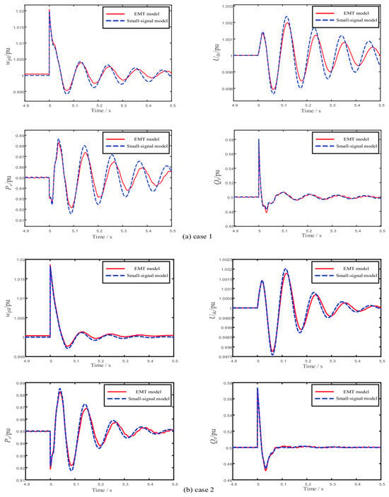
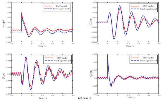
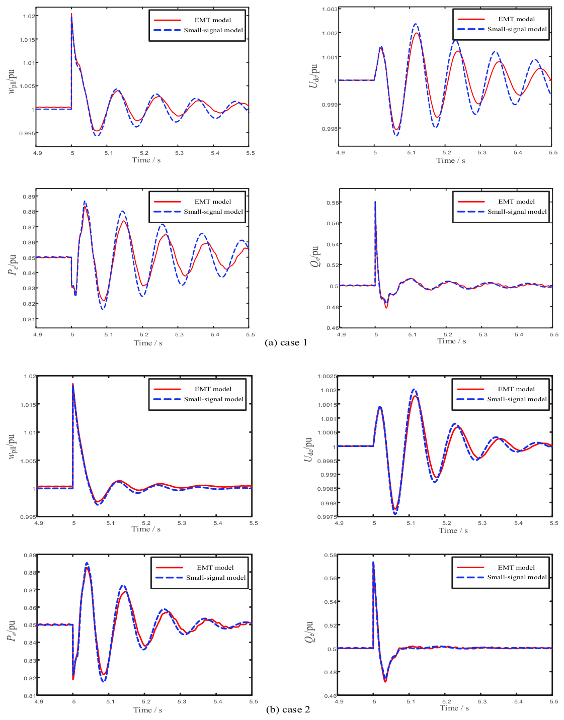
To verify the accuracy of the small-signal model, a detailed EMT model and a small-signal model of a single-MMC infinite-bus system are built based on the above derivation. The circuit parameters and control parameters of the MMC are given in Appendix A. To make the oscillation characteristics more evident, the SCR of this system is set to about 1.5, with the MMC’s active power output at 0.85 pu and reactive power output at 0.5 pu. After the system reaches steady state, a 5° phase-jump disturbance is applied to the infinite bus at t = 5 s. The response waveforms of the MMC’s PLL frequency, DC voltage, active power, and reactive power are shown in Figure 2a.

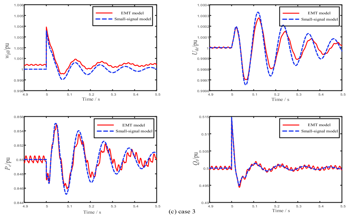
Figure 2. Time-domain simulation comparison. (a) 5° phase-jump disturbance, L_line = 0.55 pu; (b) 5° phase-jump disturbance, L_line = 0.15 pu; (c) 1° phase-jump disturbance, L_line = 0.55 pu.

To confirm that this agreement is not limited to a single operating condition, the same comparison is repeated at a representative operating point used later in the parameter studies of L_line = 0.15 pu. Under the same 5° phase-jump disturbance, the response waveforms obtained from the small-signal model and the detailed EMT model are shown in Figure 2b, confirming that the agreement between the two models is maintained under weak-grid conditions.

To further confirm that the assumed small-signal linearity holds, the baseline operating point is also verified under a smaller disturbance magnitude. A 1° phase-jump disturbance, five times smaller than that used in Figure 2a, is applied under the same baseline conditions, and the resulting response waveforms are shown in Figure 2c.

The time-domain simulation results in all three cases show close agreement between the small-signal model and the detailed EMT model, confirming that the small-signal model remains accurate across different operating points and disturbance magnitudes, and that the small-signal linearization assumption holds within the disturbance range considered. This confirms that the small-signal model can be used for the analysis in subsequent sections.

Table 1 presents the eigenvalues of the MMC small-signal model, together with the participating state variables (participation factor > 0.1), damping ratio, and frequency of each mode. For an eigenvalue λ_i = σ_i + ω_i, if ω_i = 0, then λ_i is a real eigenvalue and the corresponding mode is a non-oscillatory mode. If ω_i ≠ 0, there must be a pair of complex conjugate eigenvalues, with each pair corresponding to an oscillatory mode. Among all the modes, λ_15,16 has the smallest damping ratio (0.0280) and is therefore a weakly damped mode. Its participation factors point mainly to DC capacitor dynamics, fundamental-frequency current control, DC voltage control, and PLL control. This weakly damped mode, at a frequency of 8.7596 Hz, is taken as the object of the damping analysis in the sections that follow.

Table 1. Eigenvalues of the small-signal model of the MMC.

	Small-Signal Model Eigenvalue	State Variables with Participation Factor > 0.1	Damping Ratio	Frequency/Hz
λ1,2	−478.7 ± 1370.7i	Second-harmonic circulating current	0.3297	218.1534
λ3,4	−38.1 ± 580.4i	Second-harmonic fluctuation of submodule capacitor voltage	0.0655	92.3798
λ5,6	−40.5 ± 405.1i	Fundamental-frequency fluctuation of submodule capacitor voltage	0.0996	64.4750
λ7,8	−101.8 ± 215.6i	Fundamental-frequency current control, fundamental-frequency current	0.4271	34.3101
λ9,10	−38.3 ± 209.5i	Fundamental-frequency current control, DC component of submodule capacitor voltage, fundamental-frequency current, DC current	0.1796	33.3431
λ11,12	−64.6 ± 81.3i	Fundamental-frequency current control, fundamental-frequency current, PLL control	0.6226	12.9316
λ13,14	−27.1 ± 68.1i	Second-harmonic circulating current control	0.3703	10.8327
λ15,16	−1.5 ± 55i	DC capacitor dynamics, fundamental-frequency current control, DC voltage control, PLL control	0.0280	8.7596
λ17,18	−31.3 ± 32i	PLL control	0.6990	5.1009
λ19	−26	Reactive power control	1	/

2.3. Equation of Motion of MMC DC Voltage Control

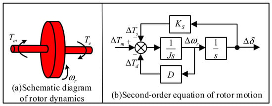
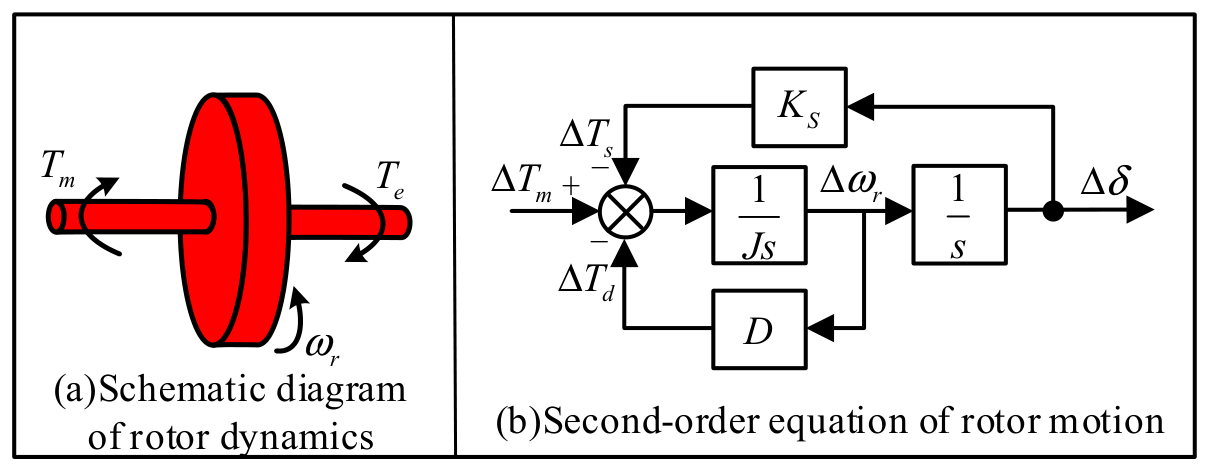
The synchronous machine is the most fundamental power generation unit in power systems and is widely used in hydroelectric and thermal power generation systems. Figure 3a shows the rotor dynamics of a synchronous machine: in steady state, the mechanical torque T_m and the electromagnetic torque T_e are equal, and the rotor speed ω remains constant. When T_m and T_e are unbalanced, the rotor speed changes. The relationship between the unbalanced torque and the speed can be expressed by Equation (49).

$$J{\displaystyle \frac{d\Delta \omega }{\mathit{dt}}}=\Delta T_m-\Delta T_e$$

(48)

Figure 3. Schematic diagram of the rotor dynamics of a synchronous machine.

This equation corresponds to the second-order rotor equation of motion shown in Figure 3b. Figure 3b shows that the difference between T_m and T_e passes through an inertia element to form the rotor speed, which then passes through an integration element to yield the power angle. The product of the speed and the damping coefficient D forms the damping torque T_d. The product of the power angle and the synchronizing coefficient K_s forms the synchronizing torque T_s. The sum of the damping torque and the synchronizing torque forms the electromagnetic torque T_e of the synchronous machine.

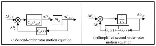
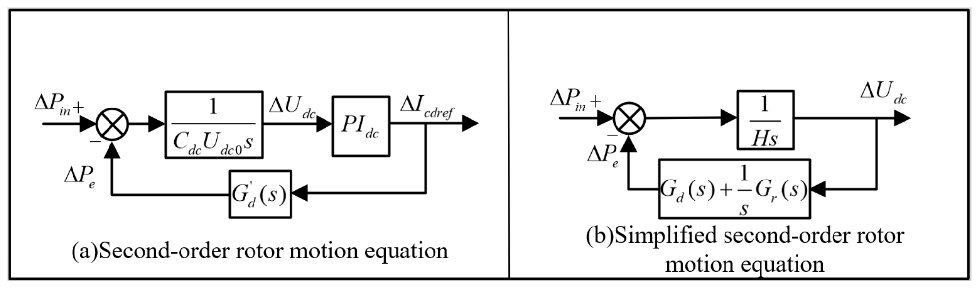
The detailed block diagram of the second-order DC voltage control loop of the MMC is shown in Figure 4. Here, G’_d(s) is the transfer function from ΔI_cdref to ΔP_e, and PI_dc is the PI element of the DC voltage control. The difference between the active power input and output on the DC side passes through the DC capacitor to produce a DC voltage deviation. The DC voltage controller then acts on this deviation to adjust the MMC output power, thereby keeping the DC voltage unchanged.

Figure 4. Schematic diagram of the dynamic characteristics of DC voltage control [24].

Comparison with the second-order rotor equation of motion of a synchronous machine reveals that the MMC’s DC voltage control exhibits similar characteristics. When the input and output power of the DC capacitor are equal, the DC voltage remains unchanged. When an imbalance occurs between the input and output power, the DC voltage changes, and the DC voltage PI controller then produces a damping force and a restoring force to eliminate the steady-state error of the DC voltage. From Figure 4, the following relationship can be obtained:

$$\Delta P_{\mathit{in}}=H\Delta U_{\mathit{dc}}s+G_d(s)\Delta U_{\mathit{dc}}+G_r(s){\displaystyle \frac{\Delta U_{\mathit{dc}}}{s}}$$

(49)

$$\left\{\begin{array}{c}H=C_{\mathit{dc}}{U}_{\mathit{dc}0}\\ G_d(s)=k_{\mathit{pdc}}{G}_d^{\prime }(s)\\ G_r(s)=k_{\mathit{idc}}{G}_d^{\prime }(s)\end{array}\right.$$

(50)

where H represents the equivalent inertia coefficient, and the system damping D_e is calculated as:

$$D_e(\mathit{j\omega })=\mathrm{Re}[G_d(s)+{\displaystyle \frac{1}{s}}{G}_r(s){|}_{s=\mathit{j\omega }}]$$

(51)

3. Small-Signal Stability Analysis of MMC

3.1. Quantitative Analysis of Damping Paths

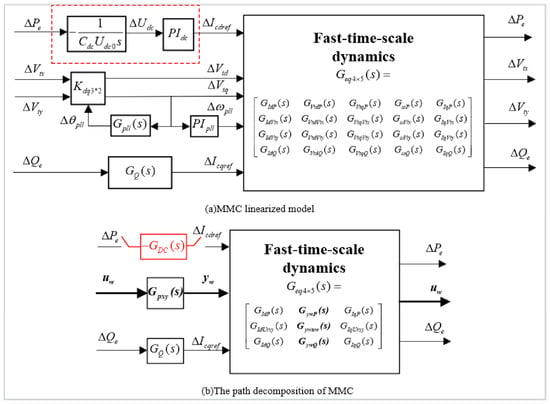
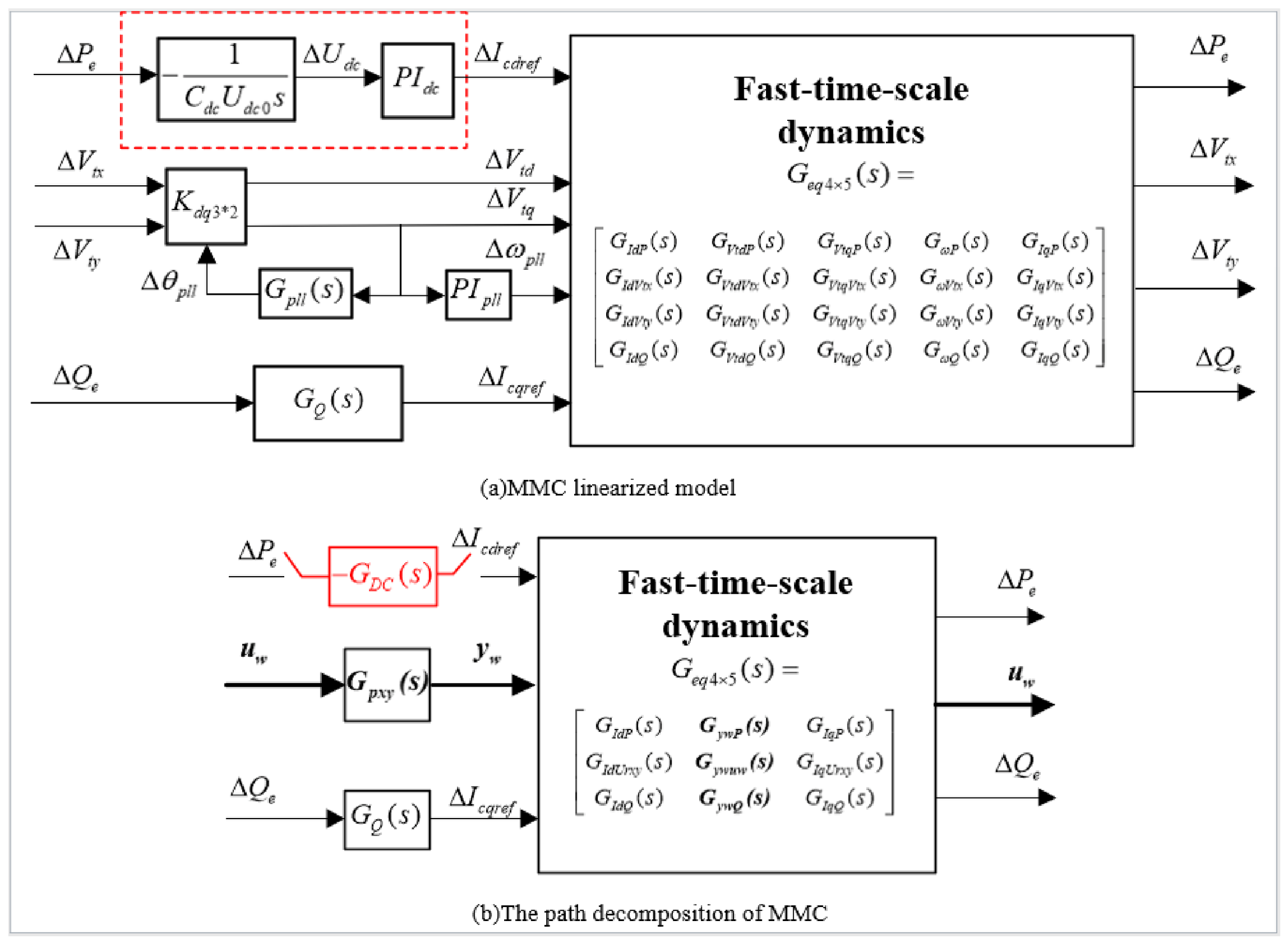
Taking the second-order DC voltage loop of the MMC as the object of study, the channels by which ΔI_cdref ultimately produces ΔP_e passing through the inner-loop control and AC network element, the reactive power control element, and the PLL control element can be divided into four categories. The first category (Path 1) passes only through the inner-loop control and AC network element, reflecting the change in output power ΔP_e caused by the dynamics of the DC voltage loop itself. The second category (Path 2) passes through the inner-loop control and AC network element together with the reactive power control element, reflecting the change in ΔP_e caused by changes in ΔI_cqref. The third category (Path 3) passes through the inner-loop control and AC network element together with the PLL control element, reflecting the change in ΔP_e caused by changes in the PLL frequency ω_pll and the terminal voltage dq-axis components V_td, V_tq. The fourth category (Path 4) passes simultaneously through the inner-loop control and AC network element, the reactive power control element, and the PLL control element. It is named the damping path corresponding to the interaction between reactive power control and the PLL.

The implementation of the damping path decomposition method follows five steps. First, the small-signal model of the MMC is linearized, as derived in Section 2.2. Second, eigenvalue and participation-factor analysis identify the target weakly damped oscillatory mode, as shown in Table 1. Third, the linearized block diagram is reorganized to construct the four damping paths, as shown in Figure 5. Fourth, the damping contributed by each path is calculated from the phase of the path-induced active-power disturbance ΔP_e relative to the DC voltage disturbance ΔU_dc, following the criterion detailed in Section 3.2. Fifth, the four path-wise contributions are superposed to obtain the total system damping D_e. This sequence is illustrated in the subsections that follow.

Figure 5. Linearized model of the GFL MMC.

To further distinguish the above four categories of paths, the linearized model shown in Figure 5a can be reorganized into the form shown in Figure 5b. Denoting the input of the PLL control element as u_w = [ΔV_tx, ΔV_ty]^T and the output as y_w = [ΔV_td, ΔV_tq, Δω_pll]^T, the active power output of the MMC can be expressed as:

$$\Delta P_e=\underset{\Delta P_{e\_\mathit{self}}}{\underbrace{G_{\mathit{IdP}}(s)\Delta I_{\mathit{cdref}}}}+\underset{\Delta P_{e\_\mathit{en}}}{\underbrace{G_{\mathit{ywP}}(s)y_w+G_{\mathit{IqP}}(s)\Delta I_{\mathit{cqref}}}}$$

(52)

where ΔP_{e_self} is the active power produced by Path 1, and ΔP_{e_en} is the sum of the active power produced by Paths 2, 3, and 4.

Since the four damping paths are derived through decomposition of the system’s total damping torque coefficient, without approximation or truncation, their sum reconstructs the total damping exactly:

D_{e_all} = D_epath1 + D_epath2 + D_epath3 + D_epath4

(53)

This identity is verified numerically in Table 2, where the summed contribution of the four paths matches the directly computed total damping D_{e_all} for all tested values of K_PLL, confirming that the proposed decomposition is complete and no damping contribution is lost or double-counted among the four paths.

Table 2. Damping provided by each damping path at f under different PLL control parameters.

KPLL	De_all (pu)	Depath1 (pu)	De_en (pu)	Depath2 (pu)	Depath3 (pu)	Depath4 (pu)
0.50	1.548	2.429	−0.881	0.769	−0.308	−1.342
0.75	0.857	2.429	−1.572	0.769	−0.518	−1.823
1.00	0.629	2.429	−1.8	0.769	−0.685	−1.884
1.25	1.024	2.429	−1.405	0.769	−0.749	−1.425
1.50	1.740	2.429	−0.689	0.769	−0.715	−0.743
1.75	2.406	2.429	−0.023	0.769	−0.638	−0.154

It should be noted that this exact summation is an algebraic consequence of the decomposition itself. The EMT simulations in Section 4 validate the overall system response and predicted trends, while the damping values assigned to each path reflect analytical attribution.

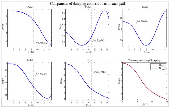
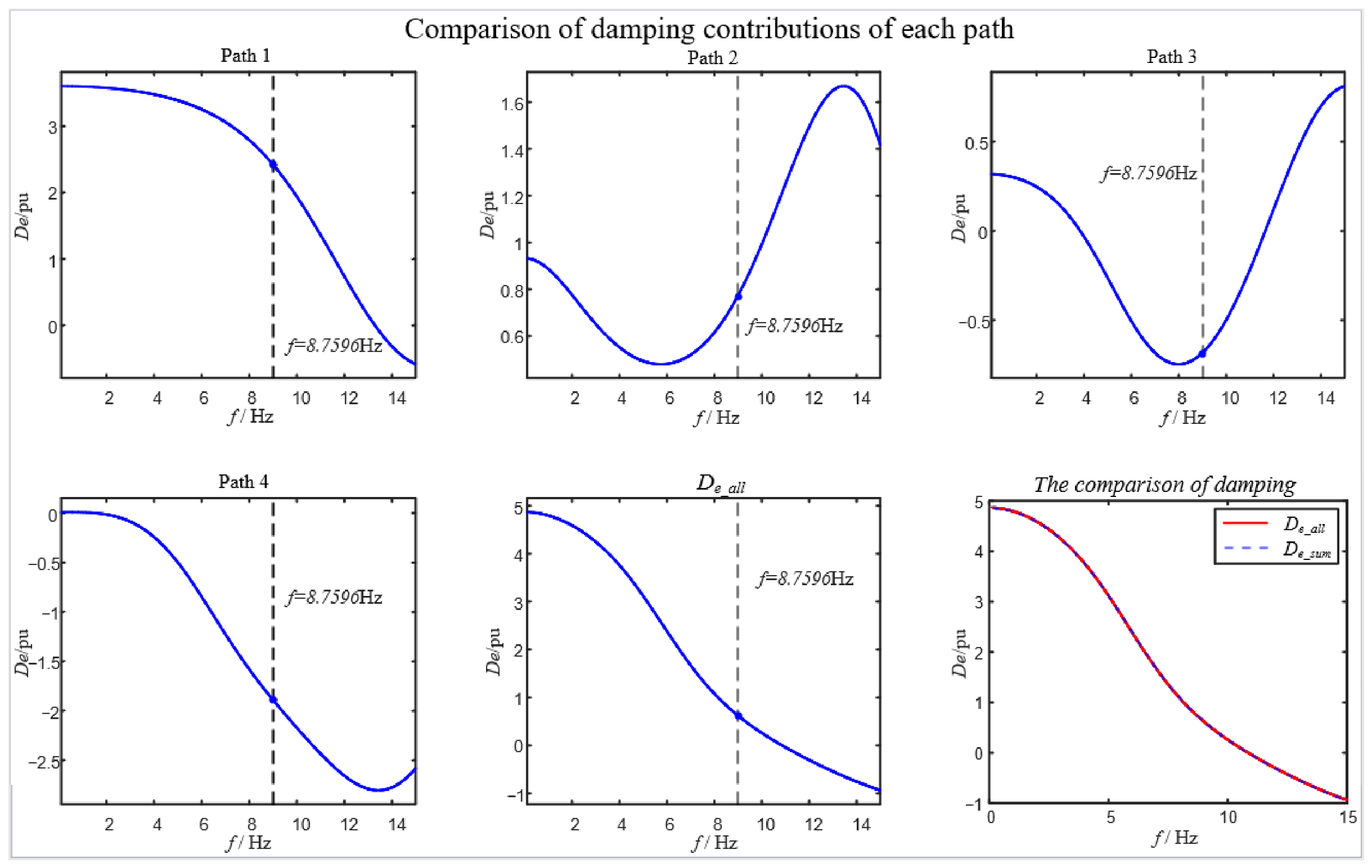
The MMC system studied in this paper exhibits an oscillatory mode at approximately f = 8.7596 Hz, as shown in Table 1. Using the circuit and control parameters given in Appendix A, the damping provided by each damping path is shown in Figure 6. As can be seen from Figure 6, at this frequency f, the MMC has insufficient damping margin and is at risk of oscillation. Paths 1 and 2 provide positive damping (2.429 pu and 0.769 pu, respectively), indicating that the MMC’s own DC voltage control and reactive power control are not the dominant sources of negative damping. Paths 3 and 4, by contrast, provide substantial negative damping (−0.685 pu and −1.884 pu, respectively), yielding a total damping of only 0.629 pu at f. Thus, PLL control, together with the interaction between reactive power control and PLL control, is the main factor causing the oscillation risk. Figure 6 also demonstrates that the four decomposed paths reconstruct the total damping D_{e_all} not only at the single target frequency, but across the entire frequency range of interest. This frequency-domain reconstruction confirms the mathematical completeness of the decomposition.

Figure 6. Damping contributions of each path.

3.2. Stability Mechanism Analysis

This section uses the damping values of each path at the key frequency point to pinpoint the main source of negative damping and clarify its mechanism. To study the influence of PLL control parameters, the proportional and integral coefficients of the PLL control are multiplied by K_PLL and K_PLL², respectively, so a larger K_PLL indicates a larger PLL bandwidth. The damping provided by each damping path at f under different PLL control parameters is shown in Table 2. As shown in Table 2, under varying K_PLL, the damping contributions from Path 1 and Path 2 remain positive and nearly constant. Path 3 consistently introduces negative damping, and so does Path 4, whose negative damping peaks around the baseline parameter and diminishes toward both sides. This shows that Paths 3 and 4 are the main causes of the low total system damping. This will be further detailed in the subsequent analysis of PLL parameter effects. The damping contributions from the four decomposed paths sum exactly to the total damping D_{e_all} at the target frequency f under all K_PLL values tested. This algebraic reconstruction verifies the internal consistency of the proposed decomposition method.

To explain why Paths 3 and 4 provide negative damping, it is necessary to return to the physical definition of damping. As shown earlier, the DC capacitor power balance equation has the same form as the speed equation of motion of a synchronous machine rotor. Accordingly, the active power disturbance ΔP_e can be decomposed into a synchronizing component in phase with ΔU_dc/s and a damping component in phase with ΔU_dc. The former changes the oscillation frequency, while the latter determines whether the oscillation decays or diverges. Therefore, whether a given path provides positive or negative damping depends on the phase of the ΔP_e it produces, at the oscillation frequency f, relative to ΔU_dc. When ΔP_e falls within the interval in phase with ΔU_dc, the path provides positive damping. When it falls within the opposite interval, the path provides negative damping.

For Path 3, its damping characteristic is determined by the phase lag of the PLL. When ΔU_dc regulates the active current through DC voltage control, it causes fluctuations in output power and terminal voltage phase, and the PLL must re-track the terminal voltage phase. Because of its finite bandwidth, this tracking process incurs a phase lag. After the PLL’s output phase error is fed back into the active current channel via the dq coordinate transformation, the phase of ΔP_e at frequency f falls into the negative-damping interval, thereby injecting negative damping into the system. For Path 4, reactive power control couples the disturbance into the PLL a second time via the terminal voltage. This is equivalent to superimposing an additional phase shift on the aforementioned phase-lag chain, causing more of the ΔP_e component to fall into the negative-damping interval. This is the main source of the decline in total system damping.

4. Influence of Control and Operating Condition

The damping path decomposition results established in Section 3, based on the damping torque analysis, show that the oscillation stability of the MMC is not determined by a single control loop, but is jointly shaped by Path 1, Path 2, Path 3, and Path 4. At the oscillation frequency f, Paths 1 and 2 provide positive damping, while Paths 3 and 4 provide negative damping. This negative damping is the main cause of the decline in total damping and the resulting low-damping oscillation. Building on the path decomposition in Section 3, this section quantitatively studies the influence of various factors on the four damping paths and on the total damping, from two perspectives: control parameters (Section 4.1) and operating point (Section 4.2).

4.1. Influence of Control Parameters on Damping

Control parameters directly determine the response speed, phase lag, and coupling strength among the multiple control loops of the MMC, and therefore have a significant influence on system damping. The damping path decomposition results show that changes in control parameters not only alter the magnitude of total damping, but more importantly reshape the distribution among the different damping paths. This section analyzes, in turn, the influence of PLL, reactive power control, and current inner-loop parameters on the damping of each path.

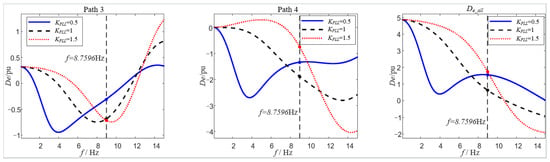
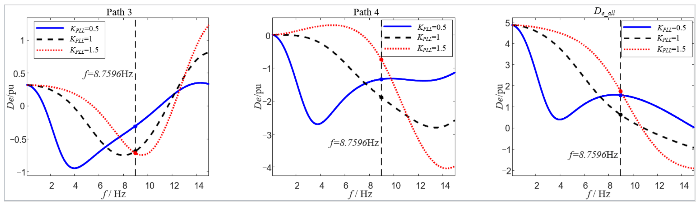
Section 3.2 has already used the damping values at the key frequency point to pinpoint the main source of negative damping and explain its mechanism. This section further examines the quantitative influence of control parameters on the damping of each path, using the curves of damping versus frequency. To study the influence of PLL parameters, the proportional and integral coefficients of the PLL control are multiplied by K_PLL and K_PLL², respectively, so a larger K_PLL indicates a larger PLL bandwidth. The variation with frequency of Path 3, Path 4, and the total damping D_{e_all} under different PLL parameters is shown in Figure 7.

Figure 7. Damping contributions of each path under varying PLL parameters.

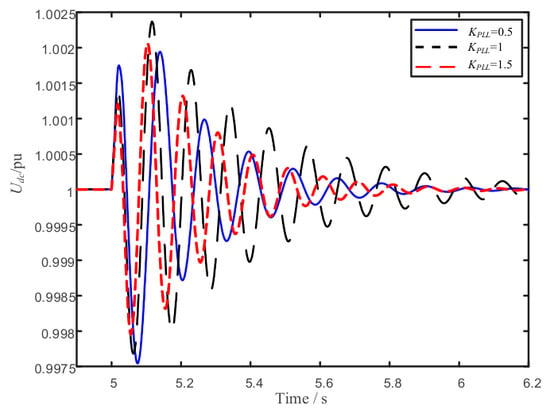
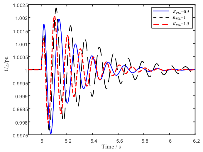
Taking all affected paths together, changing K_PLL does not change the sign of the total damping, but has a clear effect on its magnitude. The data in Table 2 show that the damping of Paths 1 and 2 remains exactly constant across K_PLL (2.429 pu and 0.769 pu, respectively). Path 3 is always negatively damped, and the magnitude of its negative damping increases with K_PLL, reaching a maximum of −0.749 pu near K_PLL ≈ 1.25 before falling back slightly. Path 4 always provides negative damping, and is most severe (−1.884 pu) near the baseline parameter (K_PLL = 1.0), increasing on either side. Of the two negative-damping paths, Path 4 dominates the trend of the total damping, causing the total damping to vary non-monotonically with K_PLL (first decreasing to a minimum of 0.629 pu at the baseline parameter, then increasing to 2.406 pu at K_PLL = 1.75). A larger PLL bandwidth is therefore not always better. Too low a bandwidth results in insufficient phase-tracking capability, while too high a bandwidth strengthens coupling with the outer loops. Only within an appropriate range can the system balance dynamic performance and stability margin. Furthermore, the time-domain simulation results in Figure 8 confirm the predicted overall trends.

Figure 8. Time-domain response comparison under varying PLL parameters.

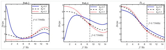
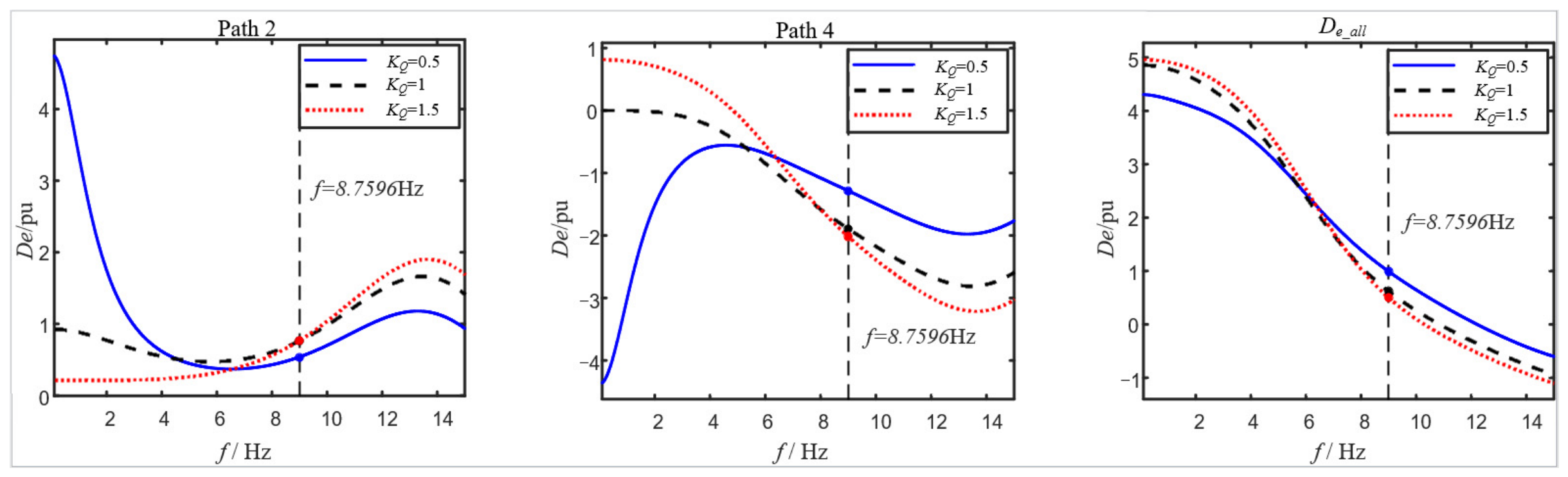
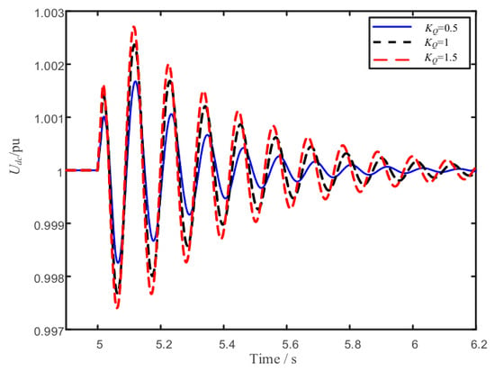
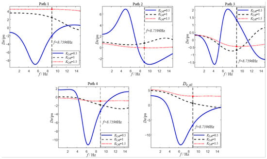
Reactive power control regulates reactive power by adjusting the q-axis current reference value. Its dynamics alter the phase relationship between AC-side voltage and current, and affect the input to the PLL via the terminal voltage feedback. Reactive power control therefore mainly influences system damping through Path 2 and Path 4, and its mechanism has similarities with that of the PLL. To study its influence, the proportional and integral coefficients of reactive power control are multiplied by K_Q and K_Q², respectively, so a larger K_Q indicates a larger reactive power control bandwidth. The damping of each path under different values of K_Q is shown in Figure 9.

Figure 9. Damping contributions of each path under varying K_Q.

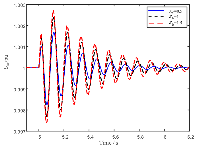
The reactive power control parameters have no effect on the damping of Paths 1 and 3, and mainly act on Paths 2 and 4. Path 2 always provides positive damping at the oscillation frequency f (approximately 0.55 pu at K_Q = 0.5, rising to approximately 0.85 pu at K_Q = 1 and 1.5), while Path 4 provides negative damping (approximately −1.3 pu, −1.9 pu, and −2.0 pu at K_Q = 0.5, 1, and 1.5, respectively). As K_Q increases, the negative damping of Path 4 becomes more pronounced, and this effect outweighs the relatively small change in Path 2. The total damping therefore decreases as K_Q increases, from approximately 1.0 pu at K_Q = 0.5 to approximately 0.5 pu at K_Q = 1.5, and is highest at the smallest K_Q considered. Unlike the PLL, a larger reactive power control bandwidth does not help suppress this negative-damping interaction. A smaller K_Q is instead more favorable for maintaining total system damping. Furthermore, the time-domain simulation results in Figure 10 verify the predicted overall trends.

Figure 10. Time-domain response comparison under varying K_Q.

The fundamental-frequency current control and the circulating current suppression control together constitute the fast-time-scale current loop dynamics of the MMC. It is a forward dynamic element shared by the damping paths associated with DC voltage control, reactive power control, and the PLL. The circulating current suppression control mainly regulates the arm circulating current via the common-mode voltage. It is used to suppress the second-harmonic circulating current and internal energy fluctuation. Unlike the PLL and reactive power control, the current loop does not directly constitute an independent external damping path. Its bandwidth and phase characteristics do, however, alter the process by which power disturbances propagate from the current reference to the AC-side output power, and can therefore still affect the equivalent damping at the frequency of interest. Although both belong to the fast inner-loop dynamics, their influence on system damping differs significantly, as discussed separately below.

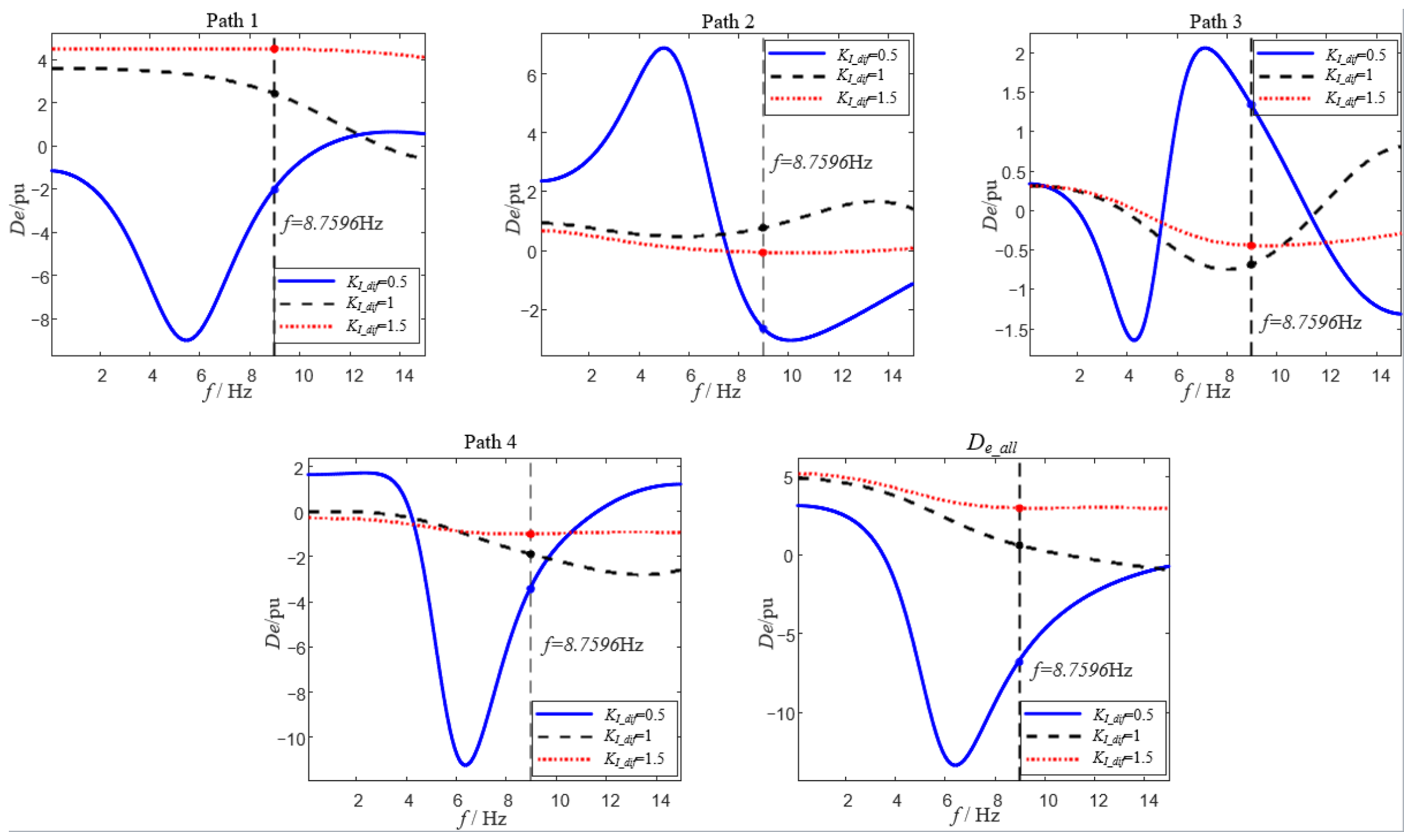
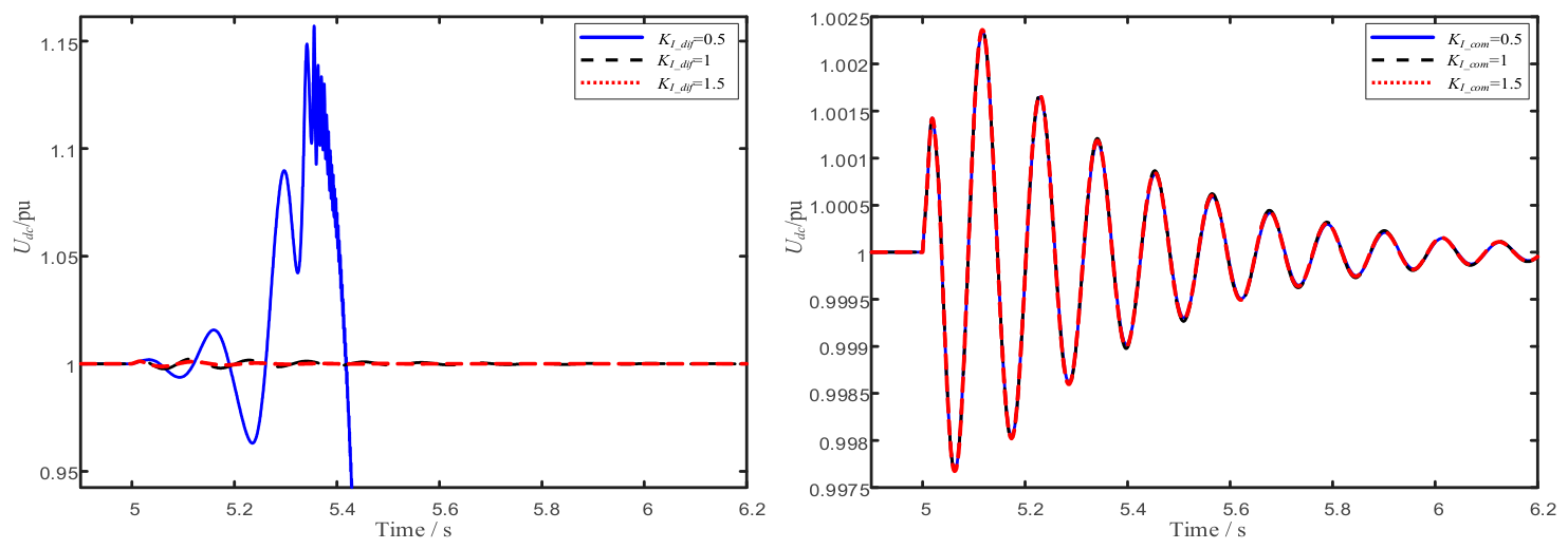
To study the influence of the fundamental-frequency current control, its proportional and integral coefficients are multiplied by K_{I_dif} and K_{I_dif}², respectively. As shown by the damping curves in Figure 11, changing these parameters mainly reshapes the magnitude-phase characteristics of the shared forward channel. At the target frequency f, the total damping varies dramatically with K_{I_dif}, from approximately −6.8 pu at K_{I_dif} = 0.5 (indicating the system would be unstable at this frequency under a low current-loop bandwidth) to approximately 0.5 pu at K_{I_dif} = 1 and approximately 3.0 pu at K_{I_dif} = 1.5. This variation is driven primarily by Path 1 and Path 4, whose damping changes from approximately −2.0 pu and −3.5 pu, respectively, at K_{I_dif} = 0.5, to approximately 4.6 pu and −0.9 pu at K_{I_dif} = 1.5. When the current control bandwidth is low, the phase lag in the current-tracking process increases. This shifts the phase relationship of the active power disturbance relative to the DC voltage disturbance, weakening the system’s damping margin near the target oscillation frequency. As the current control bandwidth increases, current-tracking capability improves, the additional phase lag in the power regulation process decreases, and the total system damping improves. However, once the current loop bandwidth is already well above the low-frequency oscillation of interest, further increasing the control parameters brings little additional improvement to the damping of the target mode. The fundamental-frequency current control therefore influences oscillation stability mainly indirectly, by changing the dynamic response of the fast-time-scale channel, rather than being a dominant source of negative damping.

Figure 11. Damping contributions of each path under varying K_{I_dif}.

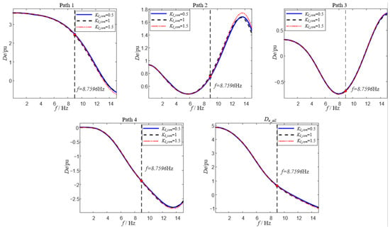
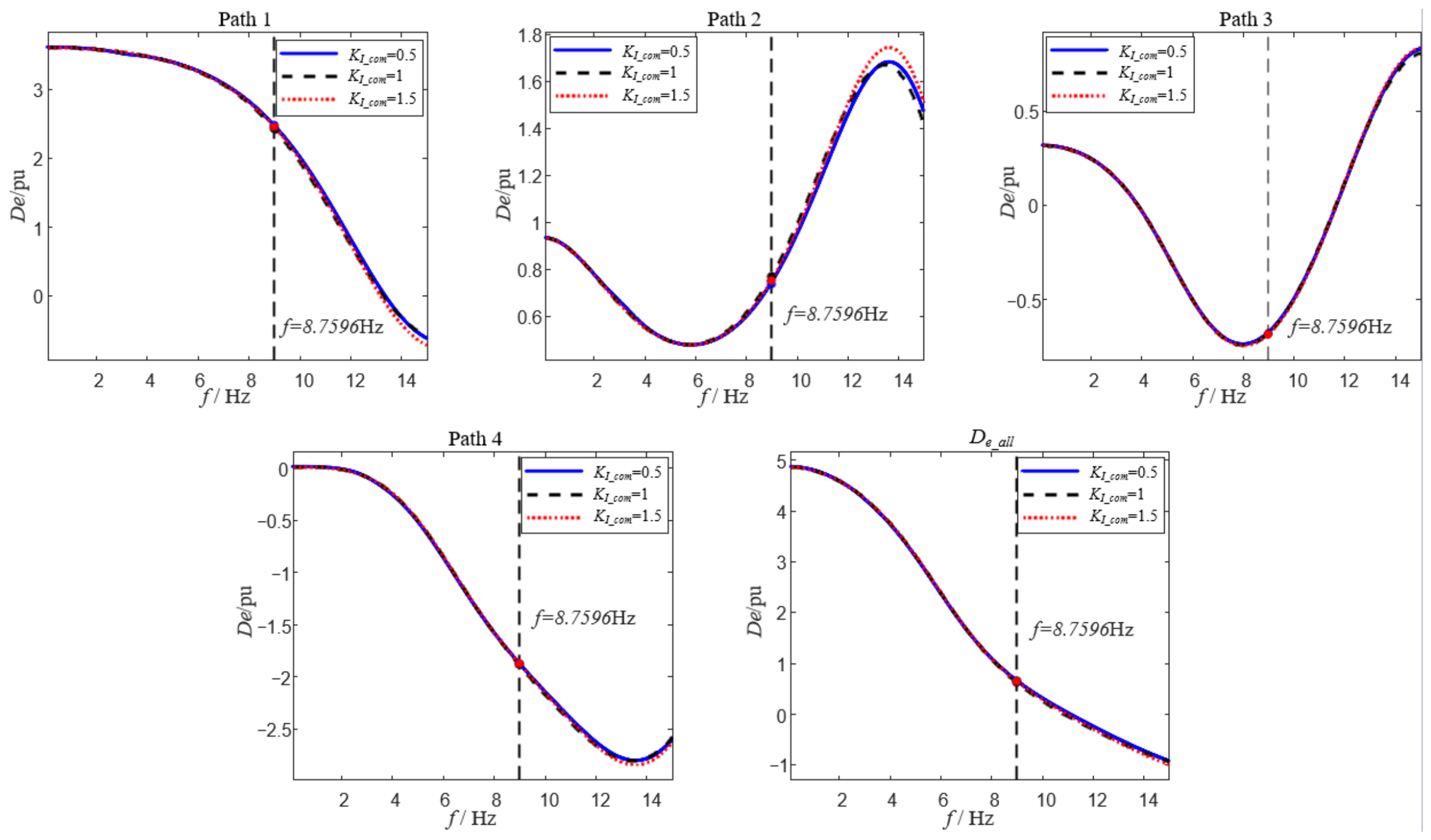
In contrast, the circulating current suppression control has a weaker influence on damping at the target oscillation frequency. Its proportional and integral coefficients are similarly multiplied by K_{I_com} and K_{I_com}², respectively. As shown by the damping curves in Figure 12, changing the circulating current suppression control parameters produces relatively small changes in each damping path and in the total damping. This is because circulating current suppression control mainly acts on the second-harmonic circulating current and arm energy balance inside the MMC, and its dominant dynamic frequency does not coincide with the DC voltage oscillation mode of interest in this paper. Moreover, this control loop does not directly participate in the regulation channel of AC-side fundamental-frequency active power, so its influence on the damping of external power exchange is mainly reflected indirectly through the arm capacitor voltage and internal energy coupling. This result is also consistent with the earlier eigenvalue analysis: although the target weakly damped mode is influenced by the fundamental-frequency current control dynamics, the main source of negative damping remains the PLL control path and its interaction path with reactive power control.

Figure 12. Damping contributions of each path under varying K_{I_com}.

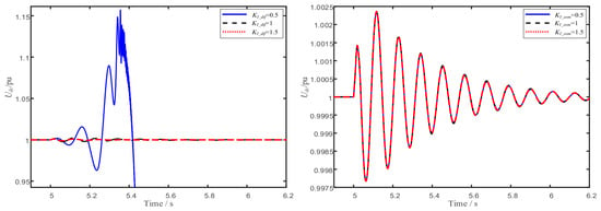
Furthermore, the time-domain simulation results in Figure 13 verify the predicted overall trends. When the fundamental-frequency current control parameters are varied, the decay rate of the oscillation in the DC voltage and related electrical quantities changes noticeably. This confirms that the fundamental-frequency current control affects the system’s damping margin. However, the oscillation frequency and its dominant character do not change fundamentally, showing that its main role is to adjust the decay characteristics of the existing weakly damped mode. When the circulating current suppression control parameters are varied, the time-domain responses differ only slightly, and the decay characteristics of the system oscillation remain essentially unchanged. This further confirms that circulating current suppression control is not a key determinant of the damping of this low-frequency oscillation mode.

Figure 13. Time-domain response comparison under varying K_{I_dif} and K_{I_com}.

In summary, current-loop parameter tuning should ensure that the fundamental-frequency current control has a sufficiently fast dynamic response, so that additional phase lag does not weaken the damping. The design focus of circulating current suppression control should instead remain on internal circulating current suppression and arm energy fluctuation control, since its influence on the sub-synchronous-band oscillation stability studied in this paper can be neglected.

4.2. Influence of the Operating Point on Damping

In addition to control parameters, the stability of the MMC also depends significantly on the operating point. Changes in the operating point alter the relative contribution of each damping path through changes in the power transmission level, voltage/current magnitudes, and the operating region of the controllers. Compared with control parameters, the operating point more directly reflects the system’s stability margin under actual dispatch. This section analyzes, in turn, the influence of grid strength, active power output, and reactive power output on the damping of each path. A change in the operating point shifts the system’s steady-state equilibrium, so for each operating condition, the steady-state point must be recomputed and the system should be relinearized before extracting the damping of each path.

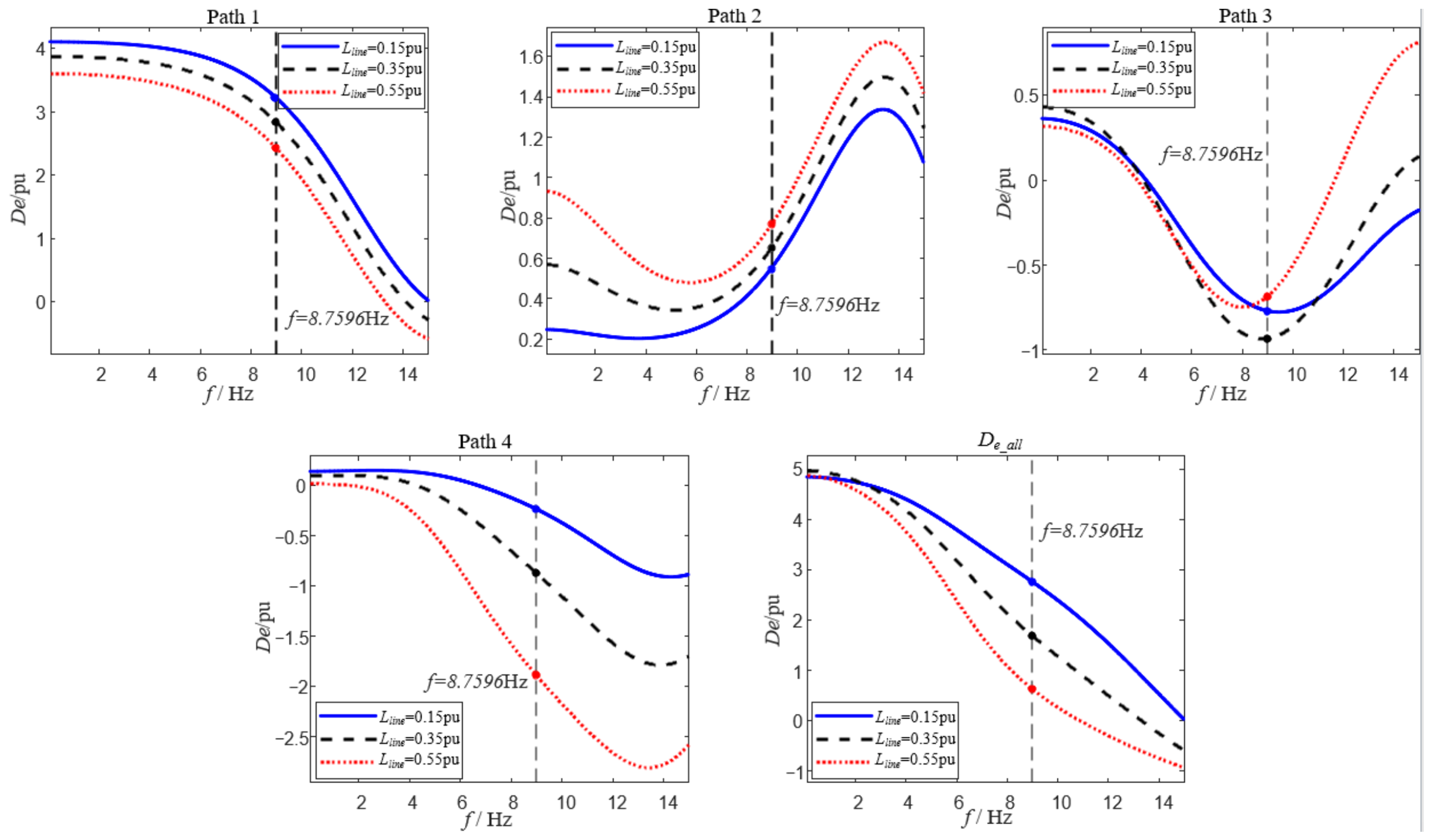
Grid strength is usually characterized by the SCR or the equivalent grid impedance. In this section, the magnitude of the external line impedance is used to represent grid strength: a smaller impedance corresponds to a stronger grid, and vice versa. For a GFL MMC, a weaker grid leaves the terminal voltage more susceptible to fluctuations in converter output power, degrades the stability of the PLL’s input signal, and strengthens the coupling among the control loops. To study its influence, the external line impedance is varied and the system is relinearized under each condition. The resulting damping of each path is shown in Figure 14.

Figure 14. Damping contributions of each path under varying grid strengths.

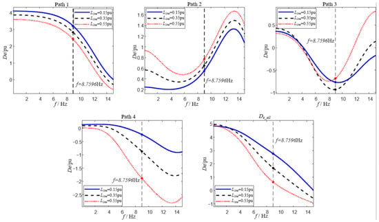
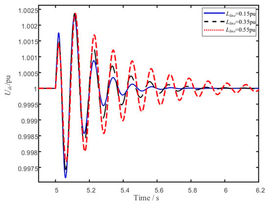
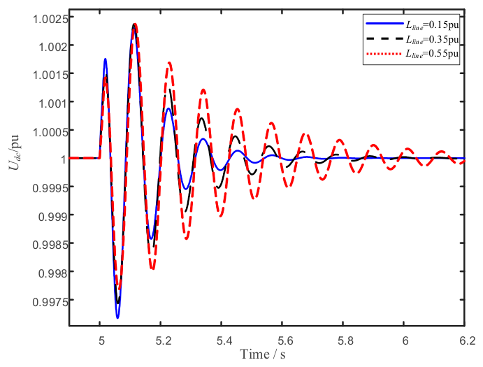
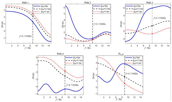
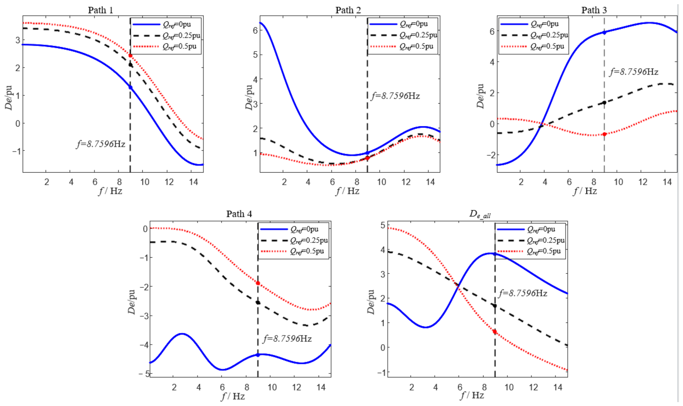
As Figure 14 shows, the total damping tends to decrease as grid strength decreases. At the target frequency f, the total damping is approximately 2.75 pu under the strongest grid condition (L_line = 0.15 pu), decreasing to approximately 1.70 pu at L_line = 0.35 pu and further to approximately 0.62 pu under the weakest grid condition (L_line = 0.55 pu). This decrease is mainly accompanied by increasingly negative damping in Path 4 (from approximately −0.22 pu to −1.88 pu as Lline increases from 0.15 pu to 0.55 pu), while the damping of Paths 1 and 2 changes relatively little. MMCs are therefore more prone to small-signal oscillation under weak-grid conditions. The root cause is not a failure of DC voltage control, but rather the amplified multi-loop coupling triggered by the PLL’s heightened sensitivity to terminal-voltage disturbances. Conversely, when the grid is stronger, the AC bus voltage is more stable and the PLL’s phase-extraction capability is more stable. The negative damping of Paths 3 and 4 weakens accordingly, and the total damping increases. Furthermore, the time-domain simulation results in Figure 15 verify the predicted overall trends.

Figure 15. Time-domain response comparison under varying grid strength.

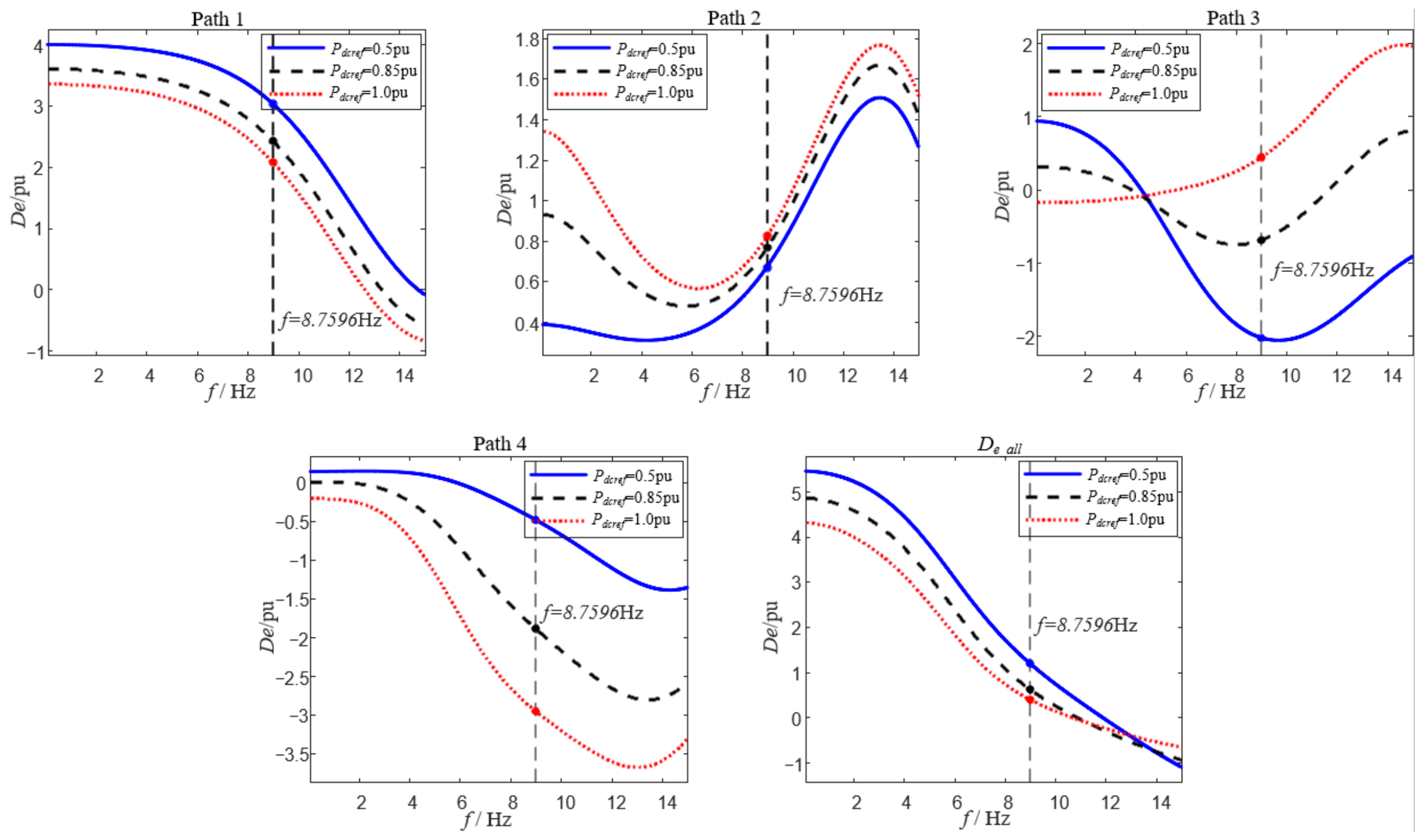
Active power output determines the MMC’s steady-state power exchange level and also alters the energy transfer relationship between the DC side and the AC side. To study its influence, the active power command is varied and the system is relinearized under each condition. The resulting damping of each path is shown in Figure 16.

Figure 16. Damping contributions of each path under varying active power output.

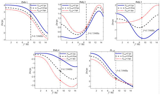
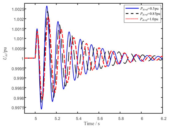
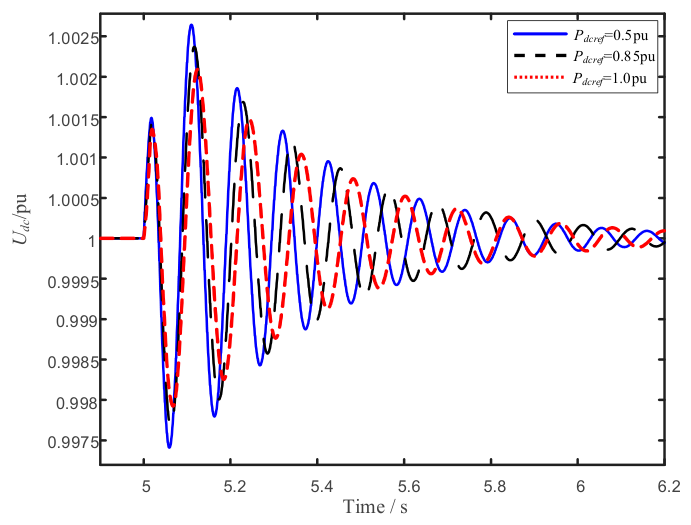
As Figure 16 shows, as active power output increases, the converter’s operating current increases, the dq-axis coupling in the power regulation process strengthens, and the dynamic coupling between the DC voltage loop and the PLL becomes more pronounced. At the target frequency, Path 4’s negative damping deepens from approximately −0.5 pu at P_dcref = 0.5 pu to approximately −2.95 pu at P_dcref = 1.0 pu, while Path 3 shifts from approximately −2.05 pu to a small positive value of approximately 0.4 pu. The negative-damping contributions of Paths 3 and 4 increase accordingly, leading to a decrease in total damping, from approximately 1.2 pu at P_dcref = 0.5 pu to approximately 0.4 pu at P_dcref = 1.0 pu. Therefore, the closer the active power output is to the rated upper limit, the more prone the system is to enter a low-damping or even marginally unstable state. At lower active power output, by contrast, the controller retains a larger regulation margin, and the total damping is relatively higher. Among the above changes, the PLL-related negative-damping paths exhibit the largest variation. Furthermore, the time-domain simulation results in Figure 17 verify the predicted overall trends.

Figure 17. Time-domain response comparison under varying active power output.

Changes in reactive power output essentially reflect changes in the q-axis current allocation and the AC-side voltage support condition. When the MMC undertakes a larger reactive power exchange, the q-axis current reference increases, the dq coupling in voltage regulation strengthens, and the interaction between the reactive power controller and the PLL becomes more pronounced. To study its influence, the reactive power command is varied and the system is relinearized under each condition. The resulting damping of each path is shown in Figure 18.

Figure 18. Damping contributions of each path under varying reactive power output.

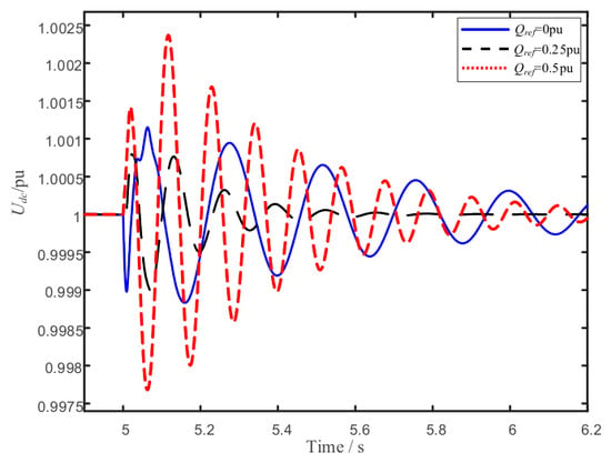
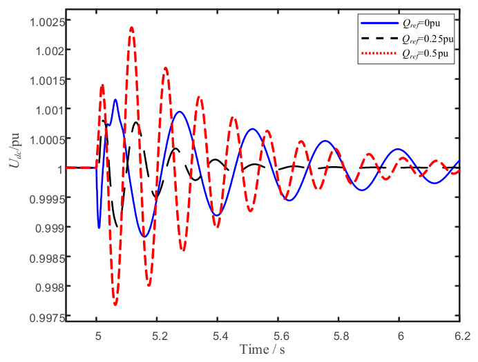
As Figure 18 shows, terminal voltage fluctuations enter the PLL’s detection element more readily as the absolute value of reactive power output increases. The negative-damping contributions of Paths 3 and 4 are amplified accordingly: Path 3 falls from approximately 5.95 pu at Q_ref = 0 pu to approximately −0.65 pu at Q_ref = 0.5 pu, while Path 4 strengthens from approximately −4.4 pu to approximately −1.85 pu. The total damping decreases correspondingly, from approximately 3.85 pu at Q_ref = 0 pu to approximately 0.65 pu at Q_ref = 0.5 pu. The negative-damping contributions of Paths 3 and 4 are amplified accordingly, and the total damping decreases. When the reactive power output is close to zero, by contrast, the AC-side voltage support burden is smaller, and the total damping is relatively higher. This trend is likewise dominated by the PLL-related paths, consistent with the effects of active power output and grid strength described above. Together, these results show that operating conditions determine the negative-damping contribution of the PLL-related paths through their effect on the strength of the voltage–power coupling. Furthermore, the time-domain simulation results in Figure 19 verify the predicted overall trends.

Figure 19. Time-domain response comparison under varying reactive power output.

4.3. Summary of Parameter Influence

In terms of control parameters, the PLL and reactive power control are the core factors affecting system damping. Path 3 and Path 4 are the main sources of negative damping. The total damping varies non-monotonically with PLL bandwidth, first decreasing and then increasing. Path 1 and Path 2 mainly provide positive damping. A larger reactive power control bandwidth, however, strengthens the negative-damping effect of Path 4 and reduces the total damping. A smaller reactive power control bandwidth is therefore more favorable for system damping. The current inner loop has a relatively secondary influence on damping when its bandwidth is sufficient. This confirms that it can reasonably be treated as a shared forward channel across the paths. However, when its bandwidth is too low and approaches the oscillation frequency, it disrupts the separation of time scales and significantly worsens system damping. The tuning of the current inner-loop bandwidth should therefore not be overlooked.

In terms of the operating point, strengthening the grid helps increase system damping, while a weak grid significantly amplifies the PLL-related negative damping. As active power output and reactive power output increase, the voltage–power coupling strengthens, the negative-damping paths’ share increases, and the total damping decreases. Parameter tuning of the MMC should therefore not merely pursue the local optimum of a single control loop, but should comprehensively consider the coupling relationships among the PLL, the reactive power outer loop, the current inner loop, and the actual operating conditions.

5. Conclusions

This paper investigates the stability mechanism of the MMC by proposing a damping path decomposition method that quantitatively decomposes the system electrical damping into four contributions: the intrinsic contribution of the DC voltage control (DVC) loop, the contribution induced by the PLL, reactive power control (RPC), and the contribution arising from the interaction between the PLL and RPC. The analysis shows that the intrinsic contribution of the DVC loop and the contribution induced by RPC are both positive, while the contribution induced by the PLL and its interaction with RPC introduce negative damping into the DVC loop and constitute the main source of the system’s low damping. The total damping varies non-monotonically with PLL bandwidth. Weak-grid and high active output conditions further amplify these negative-damping paths. This method provides an interpretation that conventional impedance-based methods cannot directly identify: the system’s low damping is not caused by overly aggressive tuning of any single controller, but arises jointly from the PLL and its interaction with reactive power control. Parameter tuning of the MMC should accordingly prioritize suppressing the PLL-related negative-damping paths, while improving the system’s damping without compromising dynamic response speed. This provides a theoretical basis for the stable operation of MMCs under weak-grid conditions and complex operating scenarios.

This study is based on a single-MMC-infinite bus system, which simplifies real grid conditions. In practice, MMCs rarely operate in isolation, and real power systems are considerably more complex. In addition, the proposed model retains only the DC, fundamental, and second-harmonic components and is therefore applicable to sub-synchronous-band oscillation mechanisms dominated by DVC, PLL, and RPC dynamics. It is not intended to capture phenomena governed by higher-order harmonic dynamics, such as internal circulating-current control interactions at the sixth harmonic and above, which lie outside the scope of the present analysis. In multi-converter and multi-machine systems, the damping paths of different MMCs may couple with one another and with synchronous-generator dynamics through the shared grid, producing interaction mechanisms beyond what a single-machine model can capture. Future work will extend the proposed damping path decomposition method to multi-converter and hybrid AC/DC systems, so as to characterize the cross-coupling of damping paths among multiple MMCs and synchronous generators under a wider range of operating and grid conditions.

References

- Cheng, Y.; Xie, J.; Zeng, C.; Yang, S.; Sun, H.; Qin, L. Comparison Study of the Wideband Oscillation Risk of MMC between Grid-Following and Grid-Forming Control. Energies 2024, 17, 2507. [Google Scholar] [CrossRef] [Scilit]
- Dang, R.; Jin, G. High-Frequency Oscillation Suppression Strategy for Renewable Energy Integration via Modular Multilevel Converter—High-Voltage Direct Current Transmission System Under Weak Grid Conditions. Electronics 2025, 14, 1622. [Google Scholar] [CrossRef] [Scilit]
- Yang, X.; Fu, X.; Xiang, J. Dissipating Energy Flow Analysis of a Constant Power-controlled MMC for Sub-synchronous Oscillation. In Proceedings of the 2024 IEEE 8th Conference on Energy Internet and Energy System Integration (EI2), Shenyang, China, 29 November–2 December 2024. [Google Scholar] [CrossRef] [Scilit]
- Wang, S.; Preece, R.; Barnes, M. Small-Signal Stability of Grid-Connected MMC-HVDC Systems: Impact of PLL Bandwidth and SCR. In Proceedings of the IET Powering Net Zero 2024 (PNZ 2024), Birmingham, UK, 3–6 December 2024. [Google Scholar]
- Wang, Y.; Xu, Q.; Guerrero, J.M. Effect of Frequency Coupling on Stability Analysis of a Grid-Connected Modular Multilevel Converter System. Energies 2021, 14, 6580. [Google Scholar] [CrossRef] [Scilit]
- Fu, Q.; Du, W.; Zheng, K.; Wang, H. Damping Torque Analysis of VSC-Based System Utilizing Power Synchronization Control. IOP Conf. Ser. Mater. Sci. Eng. 2017, 199, 012047. [Google Scholar] [CrossRef] [Scilit]
- Yuan, H.; Yuan, X.; Hu, J. Modeling of Grid-Connected VSCs for Power System Small-Signal Stability Analysis in DC-Link Voltage Control Timescale. IEEE Trans. Power Syst. 2017, 32, 3981–3991. [Google Scholar] [CrossRef] [Scilit]
- Ma, Y.; Zhu, D.; Hu, J.; Liu, D.; Ji, X.; Zou, X.; Kang, Y. Reduced-Order Modeling and Transient Stability Analysis of Grid-Connected VSC in DC-Link Voltage Control Timescale. IEEE J. Emerg. Sel. Top. Power Electron. 2024, 12, 2981–2994. [Google Scholar] [CrossRef] [Scilit]
- Lu, Y.; Liu, M.; Shao, C.; Lin, J.; Yang, Q.; Li, Y.; Du, Z. Synchronous Stability Analysis Model of Grid-following Converter Based on Singular Perturbation Method. In Proceedings of the 2024 10th International Conference on Electrical Engineering, Control and Robotics (EECR), Guangzhou, China, 29–31 March 2024. [Google Scholar] [CrossRef] [Scilit]
- Zhao, B.; Chen, L.; He, T.; Min, Y.; Li, S.; Guo, C. Corrected Complex Torque Coefficient Method for Small-Signal Stability Analysis of Grid-Connected VSC. In Proceedings of the 2021 IET Conference, Online, 14–15 October 2021. [Google Scholar] [CrossRef] [Scilit]
- Zhao, B.; Chen, L.; Min, Y.; Li, Y.; Xu, S. Corrected Complex Torque Coefficient Method for Synchronization Stability Analysis of Grid-Connected VSC. IET Renew. Power Gener. 2024, 18, 412–425. [Google Scholar] [CrossRef] [Scilit]
- Zhao, L.; Wang, X.; Jin, Z. Exploring Damping Effect of Inner Control Loops for Grid-Forming VSCs. IEEE Open J. Power Electron. 2025, 6, 1595–1608. [Google Scholar] [CrossRef] [Scilit]
- Zhao, B.; Chen, L.; Min, Y.; Yu, G.; Yin, A. Damping Analysis of Outer Control Loops and Impacts on Stability of Grid-Connected VSC. In Proceedings of the 2022 4th International Conference on Smart Power & Internet Energy Systems (SPIES), Beijing, China, 27–30 October 2022. [Google Scholar] [CrossRef] [Scilit]
- Gao, B.; Liu, Y.; Shao, B.; Ran, H. A Path Analysis Method to Study the Subsynchronous Oscillation Mechanism in Direct-Drive Wind Farm with VSC-HVDC System. Int. J. Electr. Power Energy Syst. 2022, 142, 108328. [Google Scholar] [CrossRef] [Scilit]
- Gao, B.; Liu, Y.; Shao, B.; Ran, H. A Damping-Path-Based Method for Analyzing Sub-synchronous Interaction in Renewable Energy Delivered via LCC-HVDC. Trans. China Electrotech. Soc. 2023, 38, 5572–5589. [Google Scholar] [CrossRef]
- Zhang, J.; Bu, S. Damping Contribution Analysis to Examine Subsynchronous Control Interactions Induced by PLL Control Loops in the Power Systems with Multiple Converter-Interfaced Generator. In Proceedings of the 2023 IET Conference, Chongqing, China, 3–5 December 2023. [Google Scholar] [CrossRef] [Scilit]
- Liu, Y.; Hu, J.; He, W.; Zhou, Y.; Zhan, M. Local Load Effect on the DC Voltage Control Timescale Oscillation of Voltage Source Converters. IEEE Trans. Power Syst. 2026, 41, 381–395. [Google Scholar] [CrossRef] [Scilit]
- Zhou, Y.; Miao, L.; Li, S.; Hu, J.; Zhu, D.; He, W. Mechanism analysis of interaction between synchronous condenser and VSC. CSEE J. Power Energy Syst. 2025. Available online: https://ieeexplore.ieee.org/abstract/document/11069422 (accessed on 18 July 2026). [CrossRef]
- Zheng, W.; Hu, J.; Liu, K.; Ye, Y. Interaction analysis of MTDC systems based on self-/en-stabilizing coefficients in weak AC grid conditions in DC voltage control timescale. In Proceedings of the 2021 IEEE 12th Energy Conversion Congress & Exposition-Asia (ECCE-Asia), Singapore, 24–27 May 2021; pp. 2262–2267. [Google Scholar] [CrossRef] [Scilit]
- Harnefors, L.; Antonopoulos, A.; Norrga, S.; Angquist, L.; Nee, H.-P. Dynamic Analysis of Modular Multilevel Converters. IEEE Trans. Ind. Electron. 2013, 60, 2526–2537. [Google Scholar] [CrossRef] [Scilit]
- Saad, H.; Guillaud, X.; Mahseredjian, J.; Dennetiere, S.; Nguefeu, S. MMC Capacitor Voltage Decoupling and Balancing Controls. IEEE Trans. Power Deliv. 2015, 30, 704–712. [Google Scholar] [CrossRef] [Scilit]
- Saad, H.; Peralta, J.; Dennetiere, S.; Mahseredjian, J.; Jatskevich, J.; Martinez, J.A.; Davoudi, A.; Saeedifard, M.; Sood, V.; Wang, X.; et al. Dynamic Averaged and Simplified Models for MMC-Based HVDC Transmission Systems. IEEE Trans. Power Deliv. 2013, 28, 1723–1730. [Google Scholar] [CrossRef] [Scilit]
- Chen, S.; Cheng, M.; Li, Y.; Yu, J.; Zhu, Y.; Wu, M.; Hu, J.; Yan, J. DC Overvoltage Analysis of GFM-controlled Wind Farm Connected via MMC-HVDC System Caused by Receiving-end AC Faults. In Proceedings of the IEEE IPEMC-ECCE Asia, Chengdu, China, 17–20 May 2024; pp. 966–972. [Google Scholar]
- Huang, Y.; Zhai, X.; Hu, J.; Liu, D.; Lin, C. Modeling and Stability Analysis of VSC Internal Voltage in DC-Link Voltage Control Timescale. IEEE J. Emerg. Sel. Top. Power Electron. 2018, 6, 16–28. [Google Scholar] [CrossRef] [Scilit]
Disclaimer/Publisher’s Note: The statements, opinions and data contained in all publications are solely those of the individual author(s) and contributor(s) and not of MDPI and/or the editor(s). MDPI and/or the editor(s) disclaim responsibility for any injury to people or property resulting from any ideas, methods, instructions or products referred to in the content. |
© 2026 by the authors. Licensee MDPI, Basel, Switzerland. This article is an open access article distributed under the terms and conditions of the Creative Commons Attribution (CC BY) license.