Disintegration of Liquid Jets in Grinding Cooling

Abstract

Liquid coolant jets are commonly used to remove excess heat from workpieces during grinding. There is a pressing need to reduce energy waste that contributes to environmental heat pollution and to limit the spread of oil-based coolants and mist formation. As a liquid jet issues from a nozzle and enters the surrounding air, surface instabilities develop, causing the jet to break into droplets. This breakup diminishes the jet’s ability to deliver maximum momentum to the workpiece and grinding wheel in grinding operations, thereby reducing cooling efficiency. The presence of moving ambient air near the workpiece and rotating grinding wheel further complicates cooling. First, the study investigates jet breakups in stationary air, predicting breakup lengths with reasonable agreement to experiments at varying jet velocities using the Reynolds Averaged Navier–Stokes (RANS) method equipped with Shear Stress Transport (SST) k-ω model of turbulence. The coolant jet breakup length for a jet normal to the grinding wheel is different from that for a free jet and affected by the proximity of grinding wheel to nozzle that was not evaluated in prior studies. Simulations were performed using Ansys Fluent software 2023R1, with careful tuning of numerical schemes and selection of breakup criteria. The results include analysis of jet breakup phenomena in presence of rotating grinding wheel and workpieces, determination of breakup lengths across a range of Weber numbers, and effects of nozzle design.

1. Introduction

A free-surface flow involving a liquid jet is influenced by capillary and surface tension effects as the jet exits an orifice or nozzle into ambient air, leading to its breakup into droplets. In grinding applications, jet cooling is more complex than the breakup of free jets due to the presence of a high-speed grinding wheel into which the coolant jet impinges. The developed Computational Fluid Dynamics (CFD) model is instrumental in predicting jet breakup under such conditions. This study explores the use of a Reynolds Averaged Navier–Stokes (RANS) turbulence modeling approach with Shear Stress Transport (SST) k-ω model which combines two turbulence models, namely k-ε and k-ω to predict the jet breakup length in a domain geometry representative of grinding operations.

A typical grinding process engineer overcomes coolant delivery challenges through trial and error as mathematical models are not readily available for industrial set-ups. The flexible manufacturing requires frequent and rapid change in location of nozzle, direction of jet and coolant rate that can be achieved using proposed numerical modeling. The scaling-up of the grinding speed and mass flow rate of coolant cause coolant jet to become prone to jet breakup. For moderate Weber (We) numbers, the key parameters of that breakup can be predicted by using the proposed methodology in its current form. The practitioners need reliable and rapid prediction of jet break-up using moderate amount of needed computational resources.

This modeling approach supports the development of techniques to improve jet cooling efficiency, thereby reducing energy waste, limiting the spread of oil-based coolants, and minimizing oil mist formation-a significant health and fire hazard. Efficient cooling also helps reduce thermal pollution, which is substantial in grinding operations. Proper cooling by a coherent (i.e., unbroken) jet is critical, as inadequate cooling can lead to thermal damage of precision-grind workpieces. A rapid numerical model of multiphase flow in reasonable agreement with experiments will help identify the coherence of the liquid jet and, in future it will increase its cooling efficiency in grinding operations.

Jet breakup compromises the coolant’s ability to penetrate the air layer generated by the rotating grinding wheel, thereby hindering access to the hot wheel–workpiece interface. To ensure effective cooling, the liquid jet must remain columnal over the distance from the nozzle to the grinding interface, retaining sufficient momentum to breach the rotating air layer.

Eggers and Villermaux [1] provided a detailed review of free-jet breakup phenomena, particularly the role of instabilities. In still air, a coherent jet can become disrupted by these instabilities, transitioning from a laminar to a turbulent or incoherent structure. As a result, the columnal shape of the jet may degrade leading to a loss of cooling efficiency. Webster et al. [2] showed that such loss of coherence significantly reduces cooling efficiency in grinding. Although turbulence in general enhances heat transfer, in the case of liquid jets, breakup and deflection due to air entrainment reduce the fluid’s ability to reach the target surface. Jet disintegration results in a fragmented stream composed of droplets of varying sizes, which collectively carry less volume per cross-sectional area than the original coherent jet. Despite substantial studies on free jets, the literature on impinging jets in grinding environments remain limited.

There is some disagreement in the literature regarding the physical origins of instabilities that disintegrate jets. Rupe [3] suggested that a jet with a non-uniform velocity profile at the nozzle exit will break down more easily, even in a laminar flow regime, whereas a turbulent jet can maintain its structure over a longer distance compared to a laminar one. Conversely, Debler and Yu [4] found that jets with non-uniform velocity profiles were more stable than those with uniform profiles, with stability being defined as an extended breakup length. The disintegration behavior of free liquid jets has been investigated by many authors including Lefebvre [5] and Liu [6]. The effects of turbulence on unbroken jet length have been studied by Grant and Middlemen [7], Lin and Reitz [8], McCarthy and Molloy [9], to mention a few studies. Goldstein and Leib [10] discussed the importance of linear instability theory to determine a proper causal solution to the jet noise problem.

Numerical modeling of jet behavior has been addressed in multiple studies [11,12,13,14,15,16,17,18,19,20]. One choice of computational method to predict liquid jet flow is the Large Eddy Simulation (LES) by Xiao et al. [16], while Zhao [18] introduced Detached Eddy Simulation (DES), a hybrid model popularly known to offer higher accuracy than RANS in many benchmark cases and requiring lower computational cost than LES. The LES and its variants still require substantially more refined mesh compared to RANS and remain computationally intense. On the other hand, the RANS models such as k-ε, k-ω and Transition SST models have gone through many modifications since their early days of development. Pope [17] described that the original k-ε model was accurate enough for planar jets but had inaccuracies in computing round jets. Therefore, he suggested some modifications in the transport equations and coefficients to better predict the round axisymmetric jets. Yoder et al. [18] presented the comparison between all popular RANS models by compiling their accuracy to predict the spread rates of round and planar jets. This data, however, is presented only for gas jets in gas medium. The spread rates described by Yoder et al. [18] do not relate to liquid jets in gas medium. Ghahrenmanian and Moshfegh [19] simulated round gas jets with several RANS models and evaluated their comparative efficiencies.

To model multi-phase flows, Pan and Suga [13] implemented the volume of fluid (VOF) method in combination with a Level Set function. Their analysis covered jet breakup of different regimes with We numbers ranging from 3 to 28,000. Other researchers [11,15,20] have also used the VOF–Level Set approach. Srinivasan et al. [15] examined jet breakup mechanisms and gas–liquid interface tracking. The VOF method is particularly well-suited to capture interface dynamics due to its precision in maintaining a sharp liquid–gas boundary-essential for simulating multiphase flows. The present study builds on this by identifying conditions that lead to jet destabilization and fragmentation, thereby enhancing the understanding of forced multiphase flows. Additional details on the VOF method are discussed in subsequent sections.

The Level Set Method (LSM) is a front tracking technique used in multiphase flow simulation. Osher et al. [21] developed the LSM as a Eulerian computational approach for representing and tracking evolving interfaces and geometries. This adaptable numerical method is broadly applicable across diverse fields including computational fluid dynamics, as highlighted by Osher and Sethian [22]. In this study, the LSM was used to simulate jet breakup with results that closely matched experimental observations. In the presented computations, VOF combined with LSM has been used to successfully track the interface of jet and its breakup.

To the best of the authors’ knowledge, breakup of multiphase jet flows with gravitational acceleration have not been modeled by RANS models, which are computationally less expensive than typical LES/DES methods. In general, modeling liquid jet flow poses significant challenges due to the extremely small spatial and temporal scales involved. At lower jet speeds, appropriate mesh resolution can capture breakup behavior in reasonable agreement with experiments. Sallam et al. [23] identified several mechanisms for turbulent liquid jet breakup in air, characterizing primary breakup and column length based on experimental observations. Different breakup regimes were identified [13,23], with jets with We numbers We ≤ 400 exhibiting Rayleigh-type instabilities [24].

The solver used by Pan and Suga [13] is a Navier–Stokes solver based on the Lagrangian-Eulerian scheme by Kashiwa and Rauenzahn [25]. They discussed four distinct breakup regimes based on the bulk jet speed. These regimes are called (i) the Rayleigh breakup regime, where the classic Rayleigh instability [24] for inviscid jets remains valid; (ii) the first wind-induced breakup, also referred to as the Rayleigh-like weakly turbulent regime; (iii) the second wind-induced breakup, corresponding to the turbulent breakup regime; and (iv) the atomization, or spray regime. According to Pan and Suga [13] the second regime, the weakly turbulent breakup, is different from the first one because the second regime is pertinent to turbulent jets as opposed to the first regime which is only for laminar jets. However, the linear Rayleigh-like instabilities are still dominant. For low We number jets, the authors [13] only presented jet breakup lengths for We = 3–120 whereas this study will present jets with We = 100–400 which fall within the second regime mentioned above. While Pan and Suga [13] employed a fully 3D computational domain, the current study utilizes a 2D axisymmetric domain to reduce computational complexity and still uphold reasonable agreement with experiments. The breakup process for moderate We range of 100–400 is still primarily caused by Rayleigh-type instabilities [9,13,24] for which a 2D domain is a reasonable choice [9], while for higher We numbers in third and fourth breakup regimes mentioned above, the approach needs to become three-dimensional to incorporate flow features that are pertinent to higher velocity breakup. The focus of this current study is the second breakup regime, namely, the Rayleigh-like weakly turbulent regime. The numerical model, albeit limited to moderate We numbers for now, is potentially capable of resolving all breakup regimes with upgrade to a 3D domain.

This study prioritizes breakup lengths over other jet properties such as droplet size distribution and radial expansion because of the study’s emphasis on applied engineering knowledge for grinding practitioners where breakup lengths of jets will help evaluate a coolant nozzle’s efficiency to produce coherent jet.

The study is composed as follows. Section 2 details the mathematical model and numerical approach, including the solution of the RANS equations using Ansys Fluent and the rationale for selecting the SST k-ω turbulence model. It also presents the computational domain, mesh configuration, and boundary and initial conditions used to simulate liquid jets in grinding cooling scenarios. Additionally, this section introduces the numerical methodology and provides specifications of the multiprocessor computing system. Section 3 presents numerical results along with their interpretation including model validation by comparison with experimental data and grid convergence study. Section 4 concludes the study and suggests directions for future research.

2. Mathematical Model and Numerical Methods

2.1. Governing Equations of the Mathematical Model

The momentum and continuity equations which describe the liquid jet flow are solved by adopting the finite volume method (FVM) [26]. Water is assumed to be the coolant material in this study to compare with experiments; nevertheless, the model can be straightforwardly extended to other liquid coolants.

In Ansys Fluent Version 2023R1 (Canonsburg, PA, USA) computations, gravity was enabled, and the jet is traveling in the direction of gravity to make it similar to the experiments of Sallam et al. [23].

Since the liquid jet flow is modeled as a transient problem, flow properties evolve over time. Consequently, the time derivative terms in the Navier–Stokes equations must be evaluated. Temporal discretization involves integrating each term of the discretized equations over a specified time interval. The integration of transient terms is relatively straightforward. A general expression for the time evolution of a variable, such as velocity u, is provided below:

$${\mathit{u}}^{\mathit{n}+\mathbf{1}}={\mathit{u}}^{\mathit{n}}+\Delta \mathit{t}\mathit{F}\left({\mathit{u}}^{\mathit{n}+\mathbf{1}}\right),$$

(1)

where F is the stationary part of continuity and momentum equations

An advantage of the implicit scheme (where F is calculated at time level n + 1) is its stability when using variable and relatively large time steps. In contrast, explicit schemes, which evaluate F at time level n, are constrained by the Courant–Friedrichs–Lewy (CFL) condition [27]. Ansys Fluent solves Equation (1) iteratively. Although a second-order implicit scheme could improve accuracy of solution of Equation (1), a first order implicit scheme is the only transient formulation available in Ansys Fluent for explicit Volume of Fluid (VOF) calculations of multiphase flows described in the next Section.

Originally developed by Noh and Woodward [28], Hirt and Nichols [29] and DeBar [30], the Volume of Fluid (VOF) method has become widely adopted for modeling multiphase flows [31]. In this interface-capturing technique, a volume fraction is used to represent the two immiscible fluids, such as liquid and air, with the interface modeled as a transitional blend rather than a sharply defined boundary. While the actual interface is physically sharp, the VOF method approximates it as a smeared region across several computational cells. The indicator function γ, representing the volume fraction of the liquid phase, is defined as follows:

γ = 0 for a point inside ambient gas

0 < γ < 1 for a point inside transitional region (mixture of gas and liquid)

γ = 1 for a point inside liquid

This indicator function is convected by the flow according to the transport equation:

$${\displaystyle \frac{\partial \mathit{\gamma }}{\partial \mathit{t}}}+\left(\mathit{u}.\nabla \right)\mathit{\gamma }=\mathbf{0},$$

(2)

where u is the velocity of mixture.

To improve the accuracy of interface tracking, the VOF method is coupled with the LSM in the present study. This coupling enhances the model’s capability to capture surface instabilities of the liquid jet. The LSM, a front-capturing method, solves a transport equation (Equation (2)) for a scalar quantity ϕ, which represents the signed distance from the liquid–air interface. However, the LSM is found to have a deficiency in preserving volume conservation [32]. On the other hand, the VOF method is naturally volume-conserved, as it computes and tracks the volume fraction of a particular phase in each cell rather than the interface itself. To overcome the deficiencies of the LSM and the VOF method, a coupled LSM and VOF approach is provided in Ansys Fluent and adopted in the present study.

2.2. Selection of Turbulence Model: SST k-ω

The selection of a turbulence model should be guided by the underlying physics of the flow. For free shear flows, some authors used LES [16] or DES [20] as a reasonable modeling approach across various applications. However, LES or DES require much more refined grids compared to RANS approach and require more time steps to complete solution.

Ghahrenmanian and Moshfegh [19] presented computational results for round gas jet and compared them with experiments. According to their findings, key characteristics of round jets including spread rate and centerline velocity decay were better predicted by Shear Stress Transport (SST) k-ω model. Hence, to model liquid jets in air, it is reasonable to choose SST k-ω among the variants of k-ω. According to Menter et al. [33], this model combines the advantages of free stream accuracy of k-ε model and the near wall accuracy of k-ω model. The SST model modifies the eddy viscosity expression in a manner so that it has shear stress transport capabilities nearly as accurate as Reynolds Stress Models (RSM).

The presented computations of a liquid jet in surrounding air are a combination of free shear layer (jet) far from a cooling body and near-wall boundary layer when the jet interacts with grinding wheel-workpiece area. Among the presented results, there are liquid jets that are issued from nozzles where the shear inner flow through nozzle needs to be computed. Areas of adverse pressure gradient have been observed. Considering the versatility of the problem, the SST k-ω was chosen among the RANS options. In Section 3, a comparison of different RANS models in terms of prediction of jet breakup lengths is presented.

An appropriate grid resolution, and numerical schemes were selected to achieve good agreement with published experimental data using the moderate number of computational resources. Furthermore, the interaction of the liquid jet with a rotating grinding wheel and the adjacent workpiece was modeled. Jet behavior issued from the nozzle and interaction with wheel and grinding surface was studied to evaluate the influence of grinding parameters on jet breakup. The current model provides a foundation for future studies to determine the most effective cooling techniques in grinding operations.

To validate the computational model, the study begins with simulating the disintegration of round liquid jets using a combination of structured and unstructured meshes of different sizes over a 2-D axisymmetric domain. This provides a foundational step toward analyses involving the interaction of liquid jets with grinding components such as a rotating grinding wheel, workpiece, or optimized nozzle designs which require complex, non-uniform meshes and geometrically intricate domains.

2.3. Computational Methodology

The axisymmetric and planar configurations of the FVM were employed to simulate round and planar jets, respectively. The second-order upwind scheme was selected for discretizing the momentum, turbulent kinetic energy (k), specific dissipation rate (ω) and level set function transport equations.

For an accurate tracking of the interface of the multiphase flow, the Quadratic Upstream Interpolation for Convective Kinematics (QUICK) [34] scheme was selected for the discretization in volume fraction transport across the domain. This method combines second-order upwind and central differencing techniques, offering high precision.

For pressure interpolation, Ansys Fluent offers several approaches that can be set by a user. For the Volume of Fluid (VOF) and Mixture models, Fluent theory guide [35] suggests the Pressure Staggering Option (PRESTO!).

All simulations were performed on a Dell Precision 5860 workstation with an Intel Core i9 multiprocessor. Depending on the size of the computational domain and grid, a different number of the 20 available processors was used for each simulation. All computations were conducted in a 2D domain using the double-precision solver.

2.4. Computational Domain and Grid

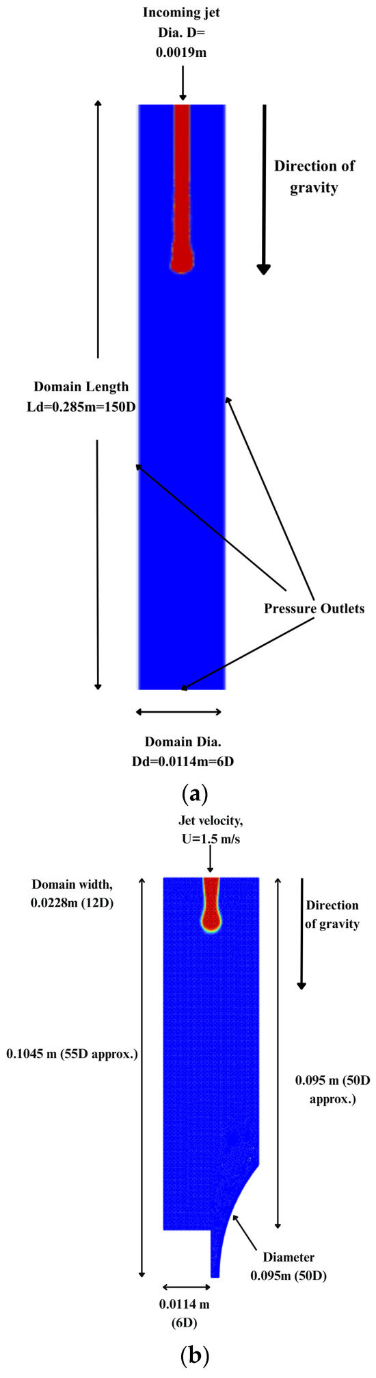
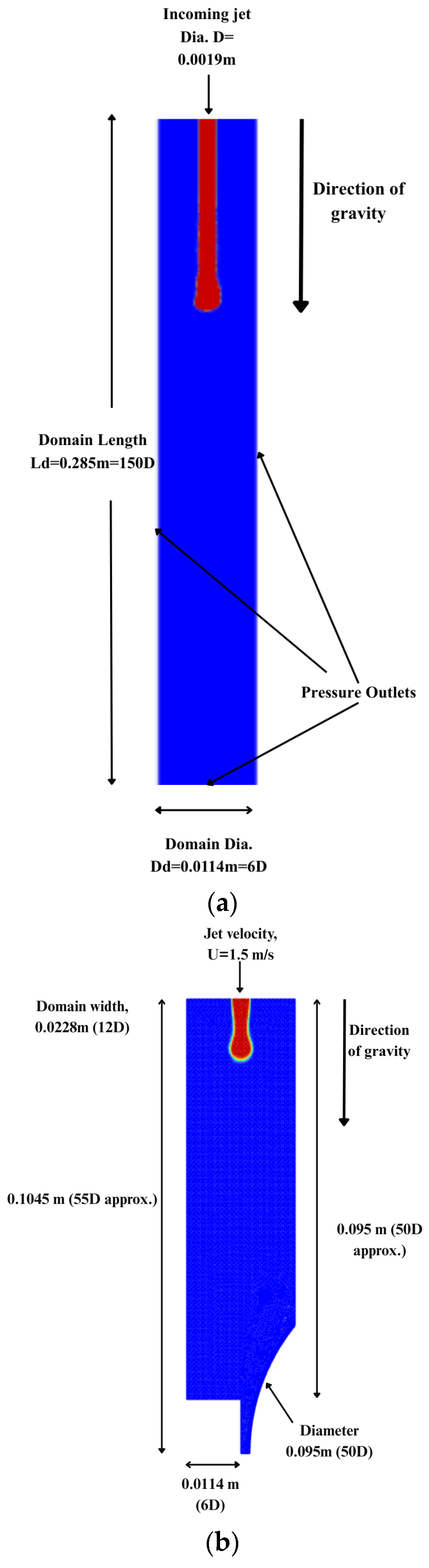
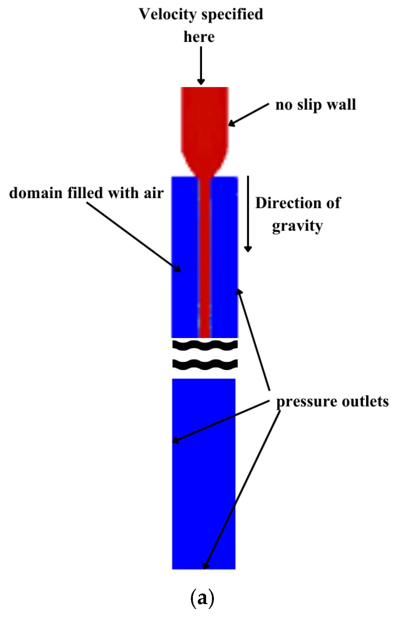
A few domains were configured to model liquid jet flow under varying conditions. For the round jet, a two-dimensional axisymmetric domain with a size of 6D × 150D was generated, where D = 0.0019 m is the nozzle exit diameter, as shown in Figure 1a. A separate domain with the same grid size was used to simulate the impingement of the liquid jet on the interface of a rotating grinding wheel and a workpiece. The rotating grinding wheel with a diameter of 50D was positioned at varying distances from the jet inlet across different cases.

Figure 1. Computational domain: (a) round axisymmetric liquid jet in air, and (b) planar liquid jet in air with rotating grinding wheel.

The domains shown in Figure 1a,b differ in height due to the inclusion of the grinding wheel in Figure 1b. For the domain in Figure 1a, axisymmetric computations were enabled in Ansys Fluent.

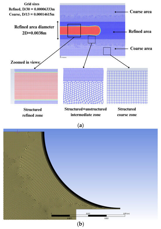
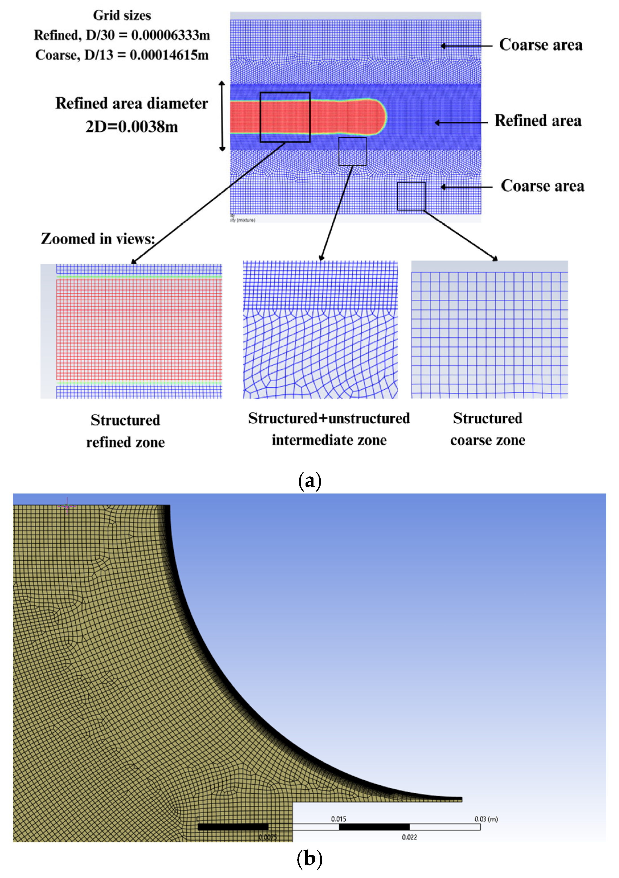
Grids were generated using the Ansys Mesh module. A combination of structured and unstructured grids with local refinement around the jet (Figure 2a) was employed to accurately capture jet breakup regimes in the simplified domain (Figure 1a). This resulted in grid cells of size 0.00014615 m × 0.00014615 m (D/13 × D/13) in the coarse region away from jet and 0.00006333 m × 0.00006333 m (D/30 × D/30) in the refined region of the domain with its radius equal to D that covers the jet. The rationale for selecting this grid size is discussed in Section 3.2: Validation of model.

Figure 2. FVM grids: (a) mixed grids for domain used for modeling of round jets; (b) unstructured mesh with inflation layer used for resolving planar flow near the wheel.

For the domain containing the rotating grinding wheel (an inflation layer was applied around the wheel (Figure 2b), and the remaining area was meshed with a mix of structured and unstructured grids. The uniform structured grid in the refined zone, shown in Figure 2a, was also used for the portion of second domain located far upstream from the wheel. This hybrid grid approach was adopted to ensure smooth transitions between different FVM meshes and to accommodate the complex geometry introduced by the rotating wheel.

2.5. Boundary and Initial Conditions

As presented in Figure 1a, the liquid jet is set up to enter the domain which is initially filled with stationary air. The blue-colored region indicates air, and the red-colored region indicates liquid coolant. The coordinate system was set to be cylindrical, having the axis at the centerline of the domain shown in Figure 1a. The sides of the domain were set to be pressure outlets for the liquid jet to spread and exit through them.

The dimensionless We number was crucial to determine the inlet velocity for a given value of surface tension. This number is defined by

$$We={\displaystyle \frac{\rho {\overline{U}}^{2}D}{\sigma }},$$

(3)

where $\rho$ is the density of inlet liquid, $\overline{U}$ is the bulk velocity (mean/average velocity) of the jet, D is the diameter of inlet (nozzle), and σ is the surface tension between coolant liquid and air.

To simulate the axisymmetric round jet using the 2D axisymmetric model in Ansys Fluent, a range of We numbers (We = 100–400) was considered. For each specified We number, the bulk (average) inlet velocity $\overline{ U}$ was calculated using Equation (3). The inlet velocity was then prescribed as a non-uniform profile to replicate the turbulent channel flow developing within a nozzle. The velocity distribution at the nozzle exit was defined by the following equation:

$$U\left(y\right) = U_{max}{\left(1- {\displaystyle \frac{2y}{D}}\right)}^{1/n},$$

(4)

where $U_{max} = \overline{U}{\displaystyle \frac{\left(2n+1\right)\left(n+1\right)}{2n^2}}$, the parameter n = 7 is typical for turbulent channel flows.

For the water jet in the presented computations, $\rho =998.3 \mathrm{k}\mathrm{g}/{\mathrm{m}}^3$, σ = 0.072 Nm, and D = 0.0019 m. The inlet velocity profile given by Equation (4) was used to simulate round liquid jets from We = 100 to We = 400. The turbulence at inlet for the jet was specified using the Intensity and Viscosity Ratio method in Fluent where the Turbulent Intensity and Turbulent Viscosity Ratio at inlet are specified at 5% and 10%, respectively.

3. Results and Discussion

3.1. Determination of Jet Breakup Length, $L_b$

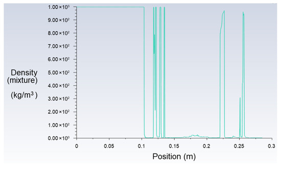
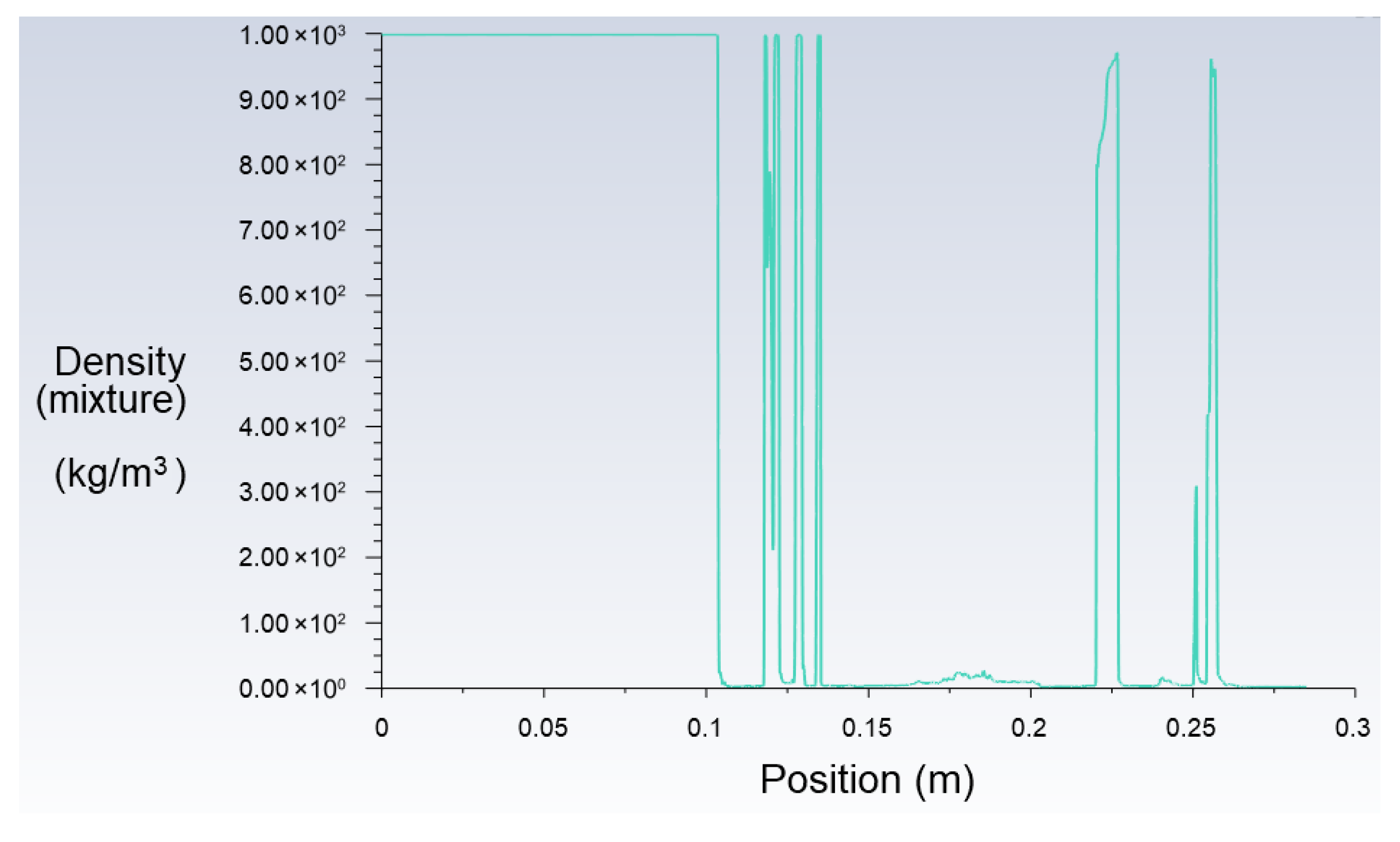
In the computational results presented, the jet breakup length, $L_b$, is defined as the axial distance from the nozzle exit to the first point where the density of the air–liquid mixture drops below 50% of the initial liquid density. This criterion provides a consistent and quantifiable method for identifying the onset of breakup in multiphase flow simulations.

Figure 3 illustrates a representative example of the density distribution along the jet axis at a specific time instant. For fully developed jets, multiple instantaneous density profiles are averaged to determine the breakup length in reasonable agreement with experiments. This averaging is necessary because the breakup point fluctuates slightly along the axis over time due to the transient nature of the flow. In the example shown in Figure 3, the jet breakup is identified at x = 0.11 m, where the mixture density first drops below 449 kg/m³. To compute an average breakup length, five consecutive frames taken at ∆t (in seconds) intervals were analyzed where the value of ∆t depends on the jet speed and domain length by relation ${\displaystyle \frac{U\Delta t}{L_D}} = 0.25$ as detailed in next sections.

Figure 3. Plot of density of water–air mixture along the jet axis.

To ensure the statistical significance of five different breakup lengths at the specified time interval, a chi-squared test by Pearson [36] was run. Considering the two categories of data, expected (averaged) and observed (actual), the χ² (chi-squared) value was calculated and compared to the χ² distribution table from Fisher and Yates [37]. The analysis yielded more than 99% probability that the data is statistically acceptable or, in other words, the uncertainties are insignificant. Also, a Python Version 3.13 (product of Python Software Foundation, the State of Delaware, USA) script is used to track the minimum and maximum breakup length after the jet is fully developed. The mean of the maximum and minimum breakup length agrees well with the average derived from five frames.

3.2. Validation of Model

Careful consideration was given to the selection of grid size. Several grid resolutions were tested to evaluate their effect on the predicted breakup length, as discussed in the previous subsection. Table 1 summarizes the computed breakup lengths for jet having We = 400, obtained using different grid sizes. For instance, a grid size D/18 in the first line of Table 1 indicates that 18 grid cells span the jet diameter D, where D = 0.0019 m. The reduction in grid sizes presented in Table 1 was pertinent to the refined zone shown in Figure 2a. The coarse mesh with its size D/13 is taken for the outer structured mesh region.

Table 1. Computed breakup lengths for different grid resolutions.

Grid Size	$\mathbf{Breakup} \mathbf{Length}, \frac{{\mathit{L}}_{\mathit{b}}}{\mathit{D}}$
D/18	165
D/22	131
D/26	113
D/30	107
D/34	107

Among the refined mesh sizes, the grid size of D/30 (0.00006333 m) was selected, as the breakup length become converged for this mesh and more refined mesh with its size D/34 (see Table 1). Also, it yielded a breakup length that closely matched experimental results [23].

When a jet of We = 390 was computed with three different time steps, the breakup length was seen to be CFL-independent (Table 2). The breakup lengths for jet described in Table 2 had a slightly lower We number than the jet in Table 1, resulting in a small reduction in ${\displaystyle \frac{{\mathit{L}}_{\mathit{b}}}{\mathit{D}}}.$

Table 2. Computed breakup lengths for different time steps.

Time Step (s)	$\mathbf{Breakup} \mathbf{Length}, \frac{{\mathit{L}}_{\mathit{b}}}{\mathit{D}}$	Maximum CFL Number
2 × ${10}^{-5}$	102	1.5
1.32 ×${10}^{-5}$	100	1.0
1 ×${10}^{-5}$	101	0.75

Table 2 confirms that the model’s prediction of breakup length does not depend on magnitude of time step for the range of CFL numbers.

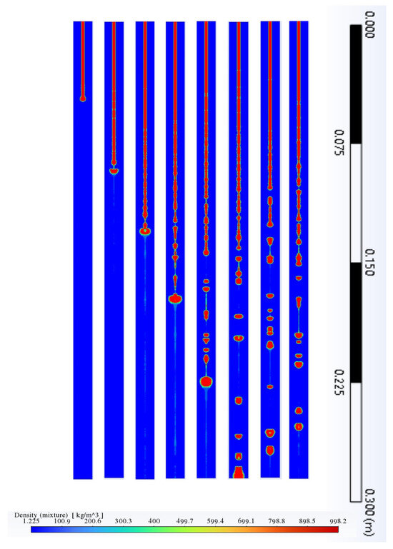
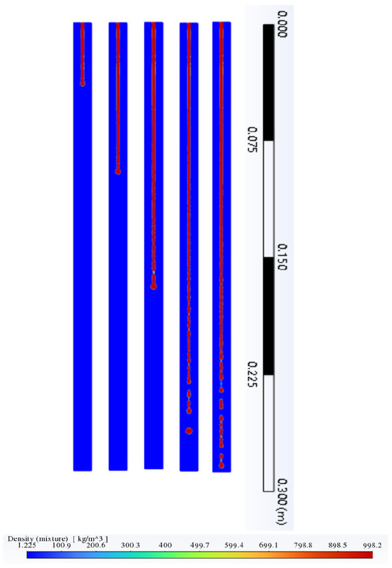
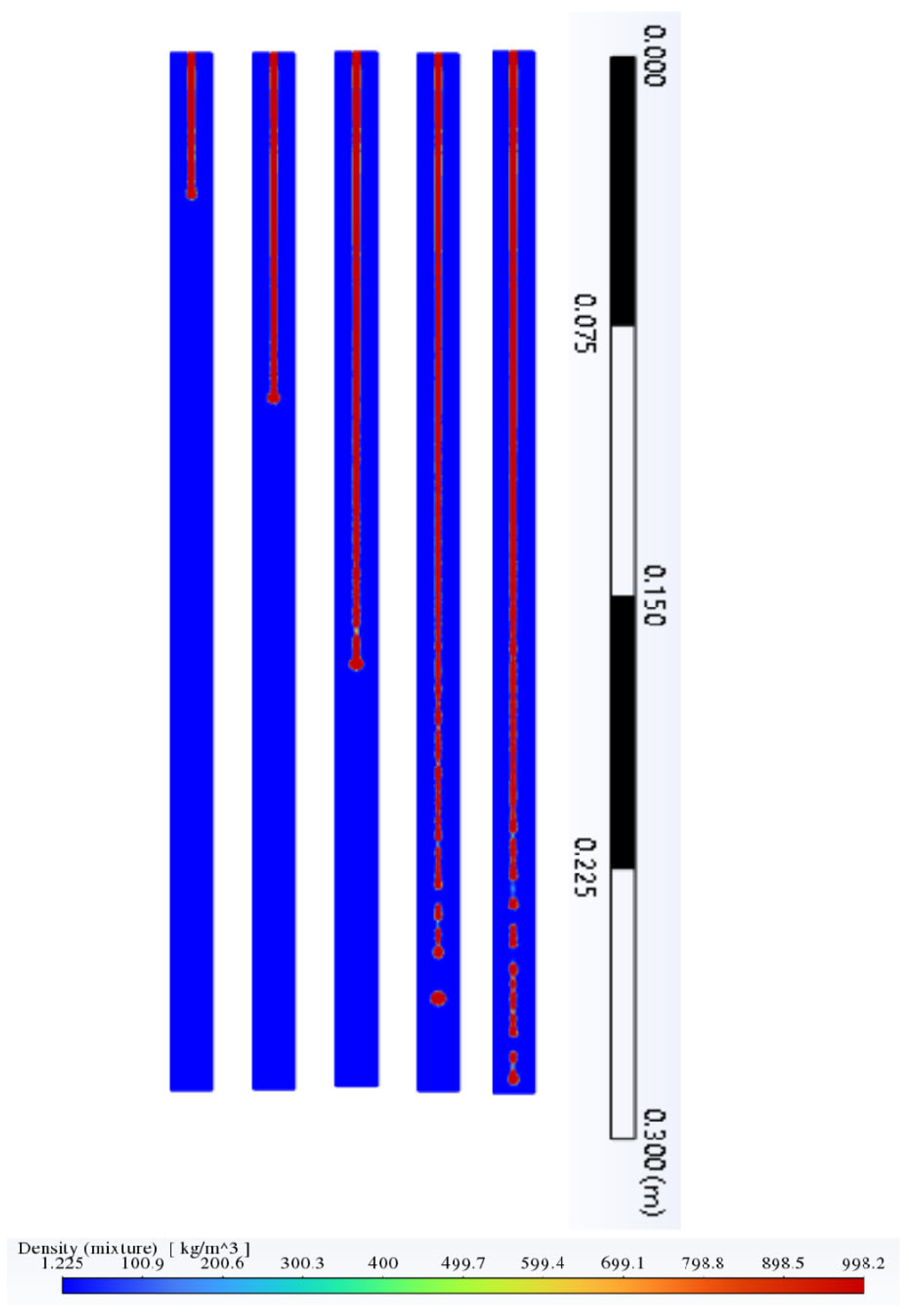
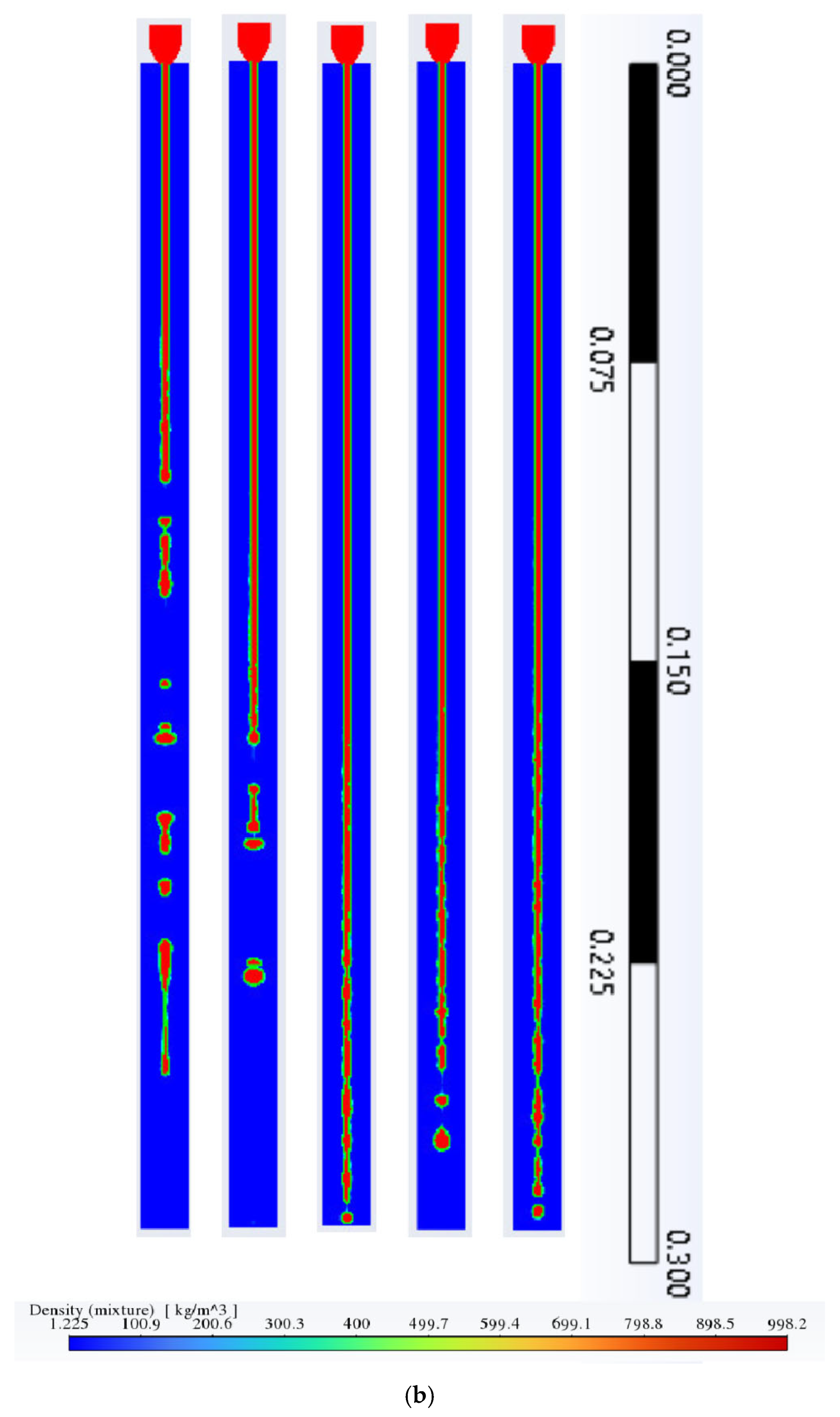
To validate the proposed computational model for jets with an initially round cross-section, simulation results (Figure 4) were compared with experimental data by Sallam et al. [23] (Figure 5). The experiment used a long cylindrical nozzle to ensure a fully developed turbulent velocity profile. A fully developed turbulent velocity profile (Equation (4)) was set as boundary condition at inlet of liquid jet. The resulting simulated jet, once fully developed, exhibited strong visual agreement with the experimental images reported by Sallam et al. [23]. The physical properties of the liquid and surrounding air (i.e., density, surface tension, and viscosity) were set to match the conditions of the experiments referenced above. The normalized breakup length, ${\displaystyle \frac{{\mathit{L}}_{\mathit{b}}}{\mathit{D}}}$, from a jet having We = 235 shown in Figure 4 was 71, while according to the experimental findings from Sallam et al. [23], ${\displaystyle \frac{{\mathit{L}}_{\mathit{b}}}{\mathit{D}}}$ was 76. Therefore, in addition to the visual similarities between experiments and simulations (Figure 5), the model predicts the jet breakup length adequately.

Figure 4. Development and breakup of round liquid jet with bulk velocity $\overline{U }$ = 2.98 m/s (We = 235), simulated with SST k-ω turbulence model. Snapshots of jet development and breakup are taken at consequent time moments with the time step Δt determined by ${\displaystyle \frac{U\Delta t}{L_D}} = 0.25$, where $L_D =$0.285 m (150D) is the length of domain. The liquid coolant (red) and ambient air (blue) are shown with the density legend (color scale).

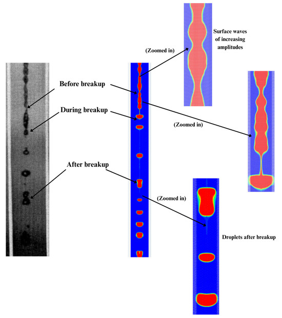
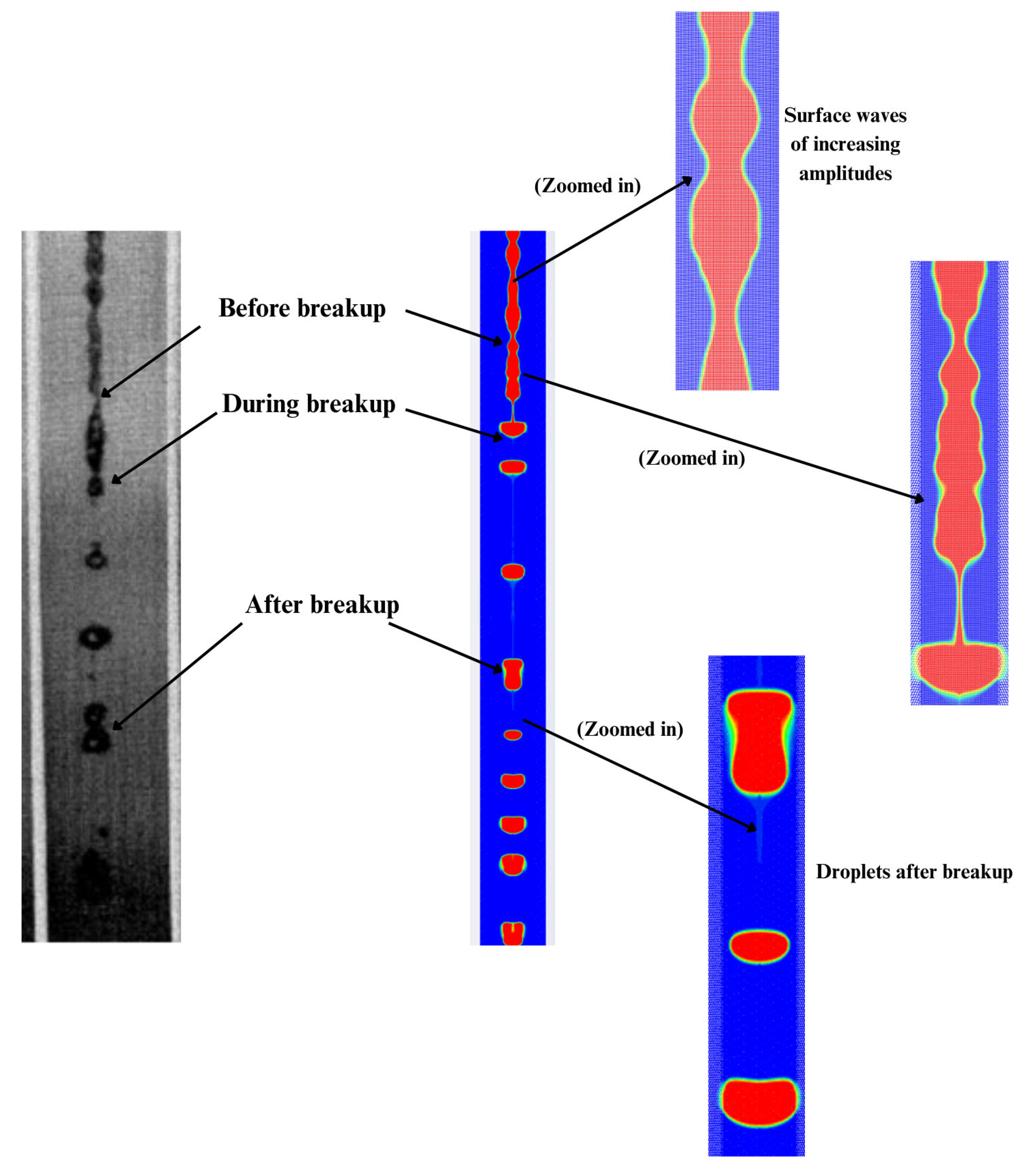
Figure 5. Jet breakup being observed in experiments [23] (left) and in computations (right) (experimental sub-figure re-used with Elsevier copyright permission).

According to Sallam et al. [23], the breakup length increases with increasing We numbers following a parabolic relationship derived through curve fitting of experimental data.

$${\displaystyle \frac{L_b}{D}}=5W{e}^{{\displaystyle \frac{1}{2}}}$$

(5)

As shown in Figure 5, the Rayleigh type instabilities [24] are evident in the simulations exhibiting patterns consistent with those reported by Sallam et al. [23].

3.3. Breakup of Round Jet and Comparison of Turbulence Models

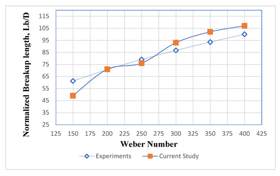
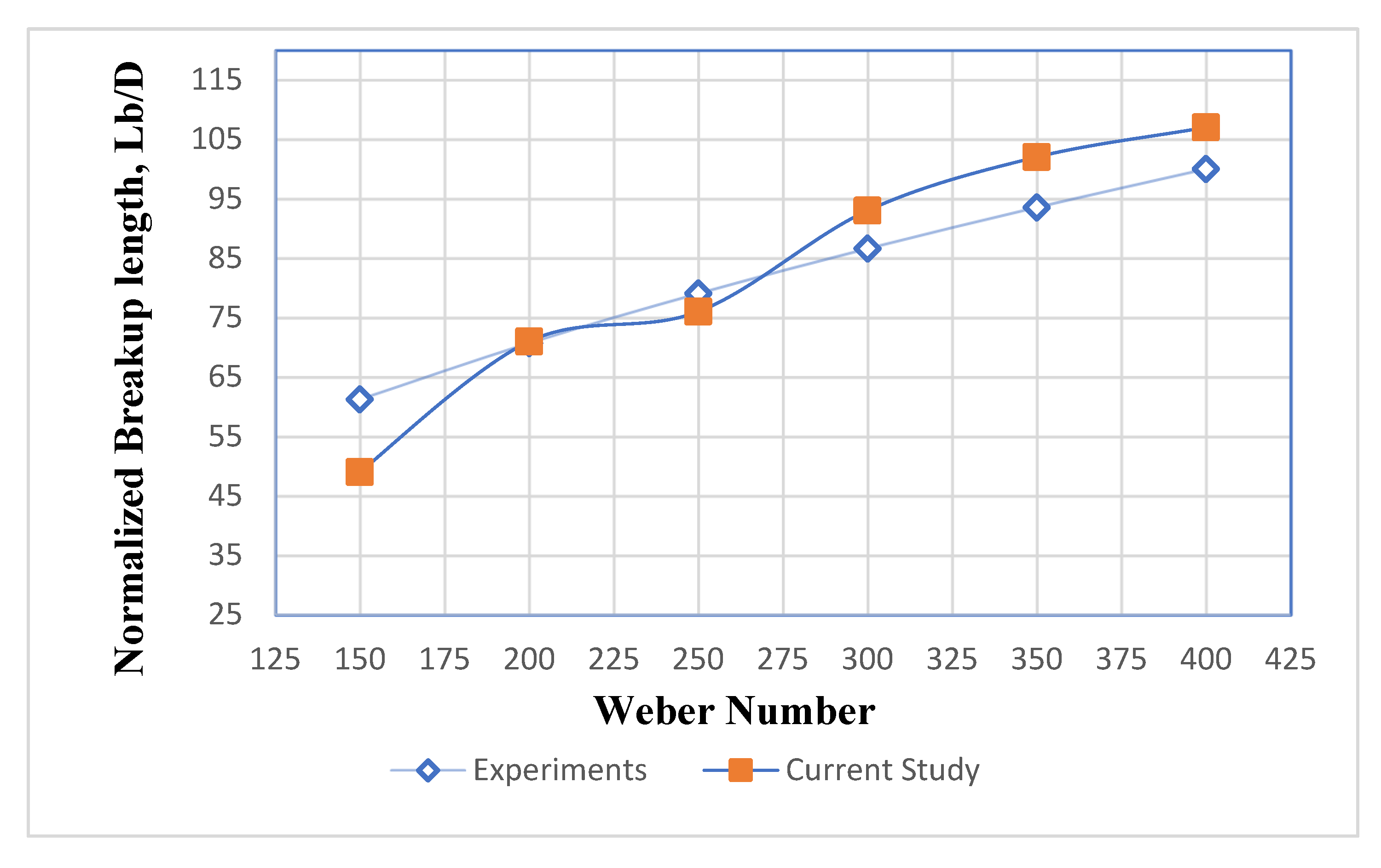
Since the breakup length predicted by numerical modeling matched the prior experimental results [23], the SST k-ω model of turbulence with the axisymmetric domain was used for simulations of round liquid jets for a range of We numbers. Figure 6 presents the breakup lengths for a range of We numbers (150–400) as well as comparisons with experimental results by Sallam et al. [23].

Figure 6. Comparison of the current SST k-ω results with experiments [23].

The predicted breakup lengths were found to closely follow the empirical relationship established by the curve fitting in Equation (5). Additionally, the simulations revealed that primary instabilities manifest as surface waves on the jet interface, as shown in Figure 5. As the amplitude of these waves grows to match the jet radius, complete disintegration occurs, which is a phenomenon previously described by Pan and Suga [13]. This type of instability that was observed to be the dominant instability, which disintegrated the jet, is called Rayleigh type instability [24].

Notably, although the simulations were conducted in a 2D axisymmetric domain, the model effectively captured the three-dimensional jet breakup phenomena, at least in terms of integral parameters such as jet breakup length. In the second Rayleigh-like breakup regime, the dominant instabilities carrying the most energy can be resolved by a 2D mechanism—see review [9]; “breakup occurs owing to the exponential growth of axisymmetric surface disturbances assumed to be infinitesimally small at the nozzle outlet. The jet breaks up once the disturbances attain the scale of the jet radius”. Simulations were performed for a range of We numbers up to 400, corresponding to various bulk velocities. Across all cases, similar breakup mechanisms driven by primary instabilities were observed, though the breakup lengths varied according to the jet’s bulk velocity (i.e., its We number), as illustrated in Figure 6.

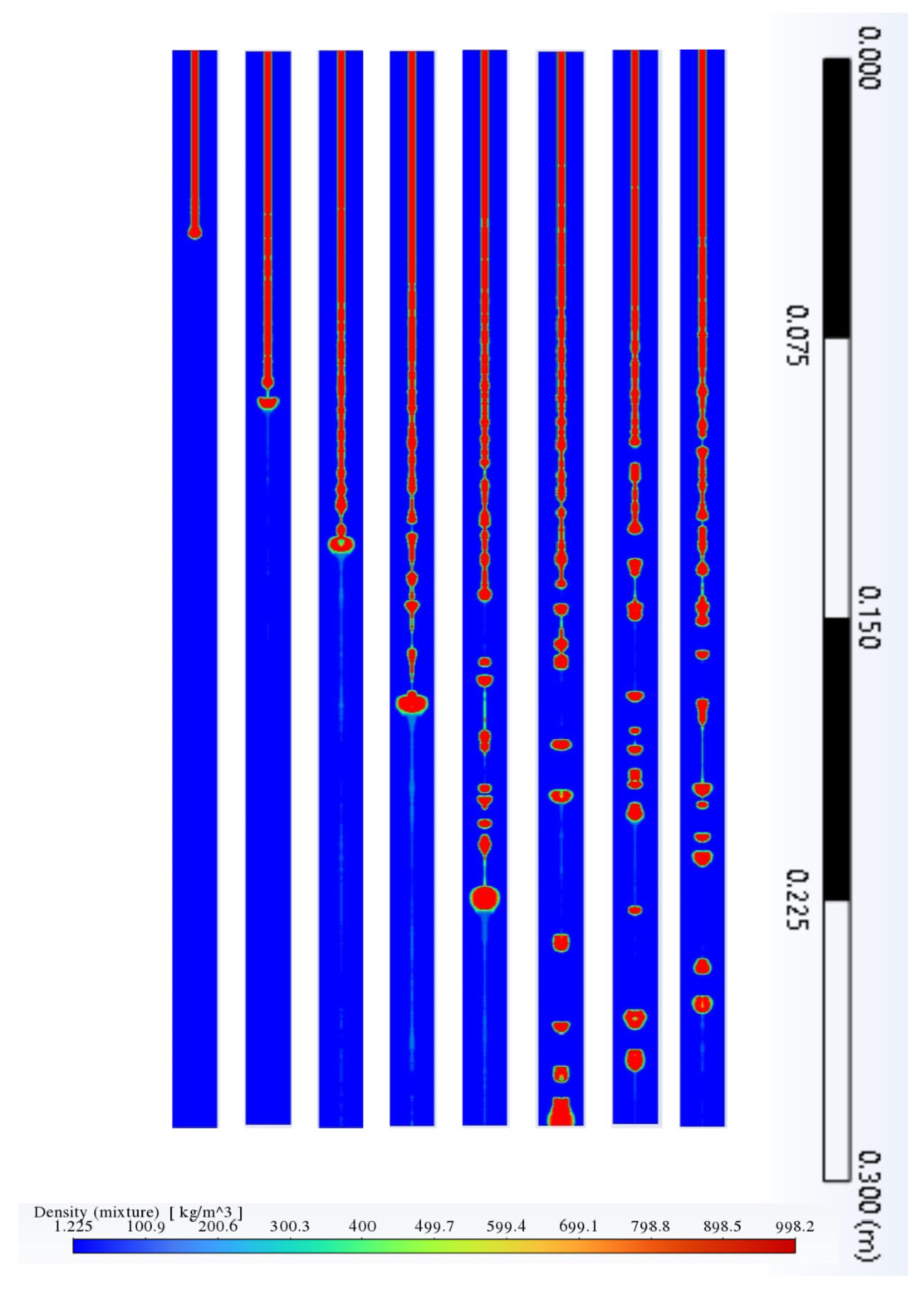
The computations for round jets having higher We numbers compared to what was presented in Figure 5 showed similar patterns of disintegration instabilities (Figure 7). The breakup length for these higher We numbers also matches the predictions from Sallam et al. [23].

Figure 7. Development and breakup of round liquid jet with bulk velocity U = 3.89 m/s (We = 400), simulated with SST k-ω. Snapshots of jet breakup are taken at consequent time moments with the time step Δt determined by ${\displaystyle \frac{U\Delta t}{L_D}} = 0.25$, where $L_D = 0.285$ m (150D) is the length of domain.

The computational results with SST k-ω model are included in Table 3 (last column) for comparison with two other RANS models. From Table 3 it is seen that for free round liquid jets, k-ε has accuracy comparable to SST k-ω model and to experiments. However, this model was not selected for present study because the SST k-ω being reportedly more accurate near walls [33], when the flow interaction with work piece and grinding wheel appears in following sections. Note that the Transition SST and k-ε models over-predict experimental break-up length for We = 400 compared to SST k-ω model. Also, the four equations Transition SST model has higher computational time compared to two-equations SST k-ω model.

Table 3. Comparison of computed breakup lengths obtained by RANS models.

	$\mathbf{Normalized} \mathbf{Breakup} \mathbf{Length} \left(\frac{{\mathit{L}}_{\mathit{b}}}{\mathit{D}}\right)$
Weber Number	k-ε	Transition SST	SST k-ω	Experiment
400	113	114	107	100
300	89	89	93	86
200	59	61	71	70
100	45	35	35	50

The We number (see Equation (3)) is a unitless parameter that includes density and surface tension of coolant liquid and therefore the results in Table 3 are pertinent to widespread Newtonian liquids (oil, water) because the We number could be calculated for a different coolant and computed results of Table 3 could be used.

3.4. Rectangular Jet

To evaluate the influence of a rotating grinding wheel on liquid jet breakup, a planar jet configuration was studied. This approach was necessary because an axisymmetric domain cannot simultaneously accommodate a cylindrical grinding wheel. Moreover, planar jets are practically relevant to grinding processes due to the common use of rectangular nozzles. Results are presented in the next sections to show how jet disintegration is affected by the presence of grinding wheel at various distances and rotational speeds.

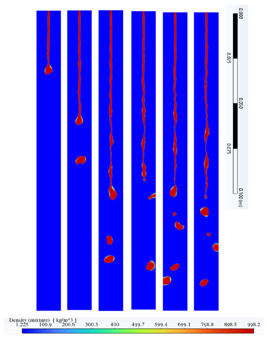
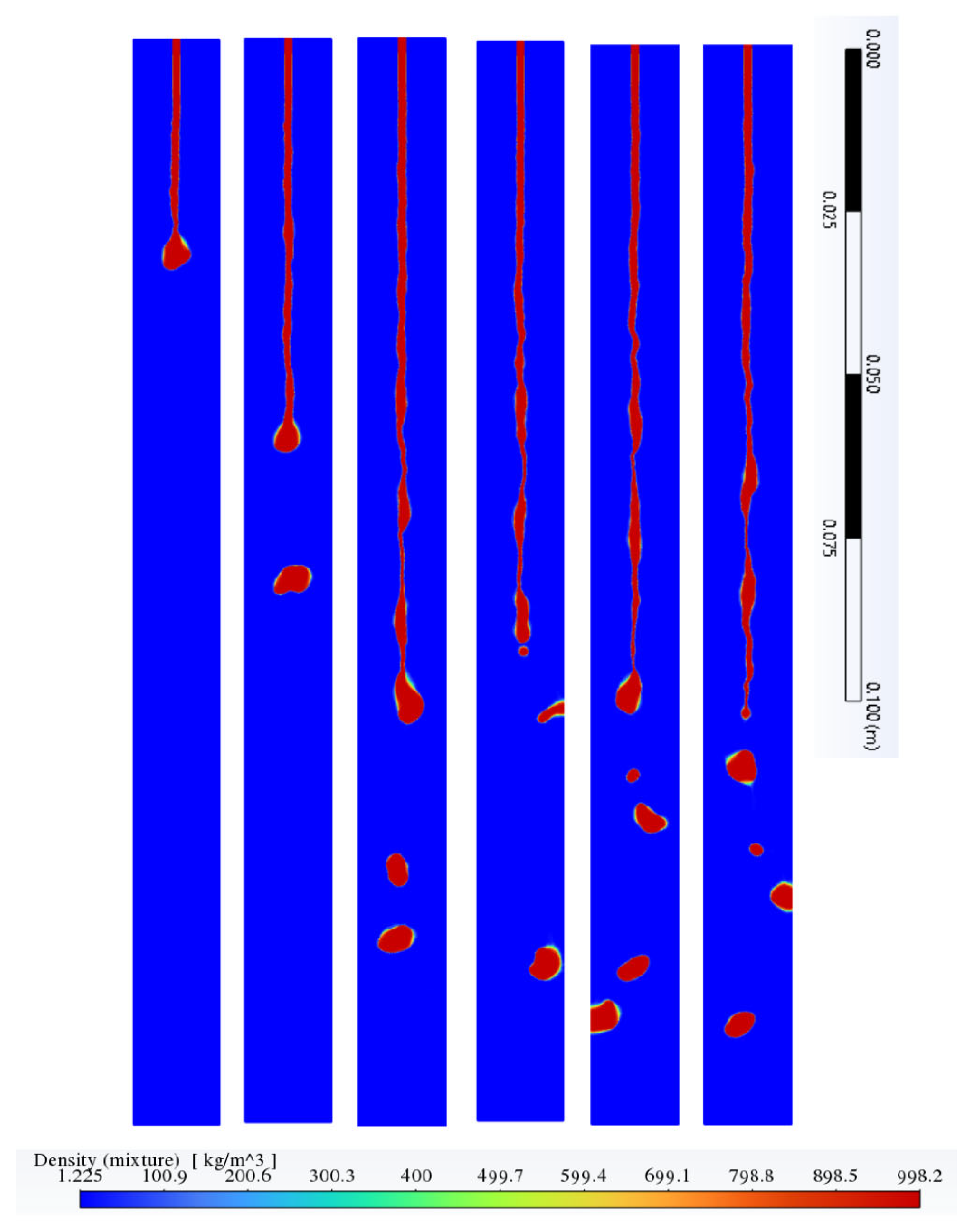
In the simulated cases, a 2D planar domain was used to model a rectangular jet. Within Ansys Fluent, this setup assumes a unit depth (1 m) in the third dimension and treats flow properties as uniform along that direction. Figure 8 shows snapshots of the development and disintegration of a planar jet issuing at $\overline{U}=U_j$ = 1.5 m/s.

Figure 8. Development and breakup of planar jet using SST k-ω model with bulk velocity U = 1.5 m/s. Snapshots are taken at consequent time moments with the time step Δt determined by ${\displaystyle \frac{U\Delta t}{L_D}} = 0.25$, where $L_D = 0.285 \mathrm{m}$ (150D) is the length of domain.

3.5. Planar Jets in the Presence of Grinding Wheel

During grinding machine operation, the high-speed rotation of the wheel interacting with coolant jet generates a substantial moving air layer around its circumferential surface. This phenomenon is commonly referred to as the air layer [38] barrier. The angle between jet and the wheel surface could vary from normal to tangential, and both limiting cases are considered in this section.

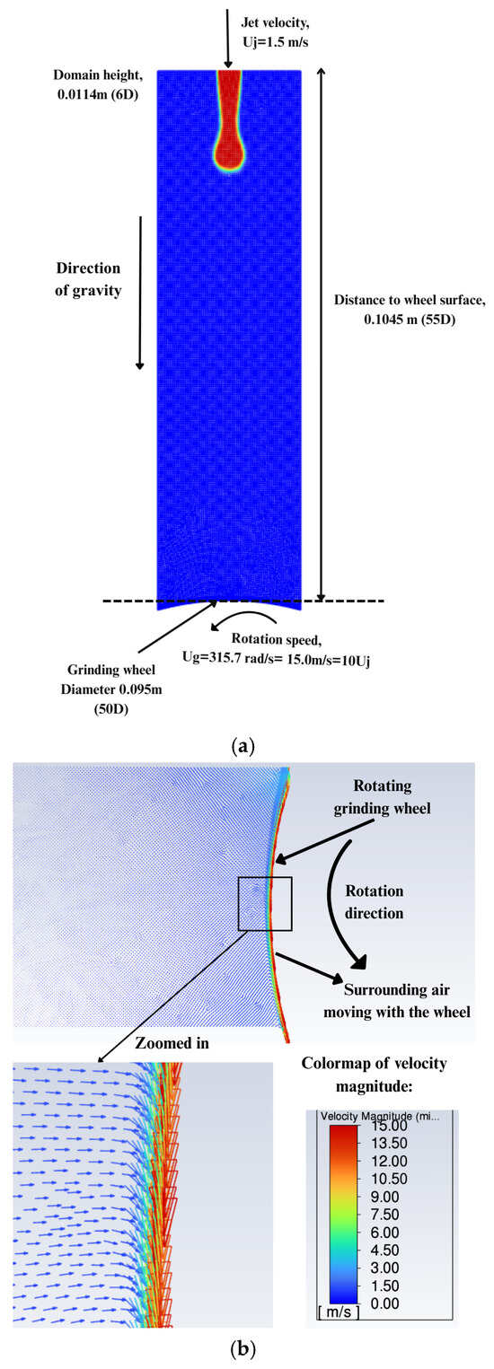
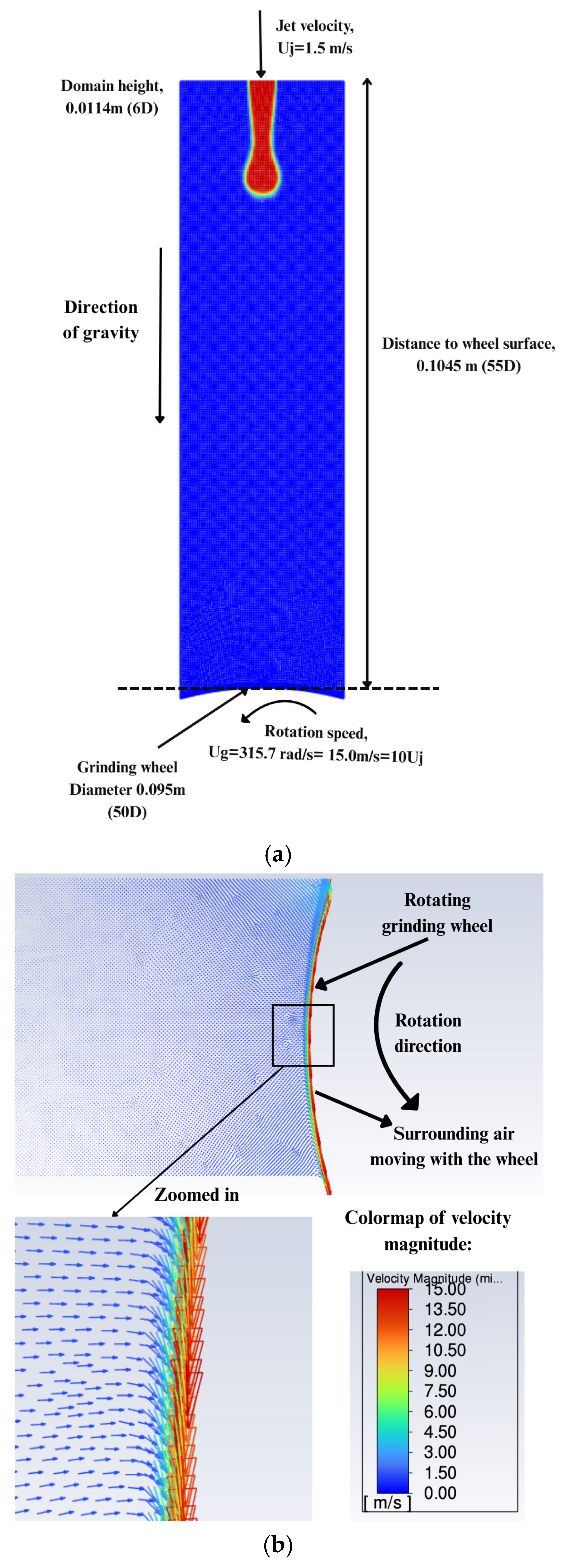
When coolant jet is applied nearly normally to the wheel surface to cool the rotating wheel, the rotating air layer acts as a crossflow opposing the incoming liquid jet [39,40]. To investigate this effect, the numerical model developed in previous sections based on the SST k-ω turbulence model was used to simulate air layer dynamics around a rotating wheel. The boundary conditions used for this simulation are described in Figure 9a,b shows how the wheel affects the motion of the surrounding air. The wheel’s linear speed was set to be ten times that of the incoming jet. A broader range of wheel-to-jet speed ratios will be explored in future studies.

Figure 9. Jet impinging normal to wheel surface: (a) domain with rotating grinding wheel without workpiece and (b) air layer around rotating grinding wheel without impinging jet.

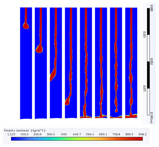
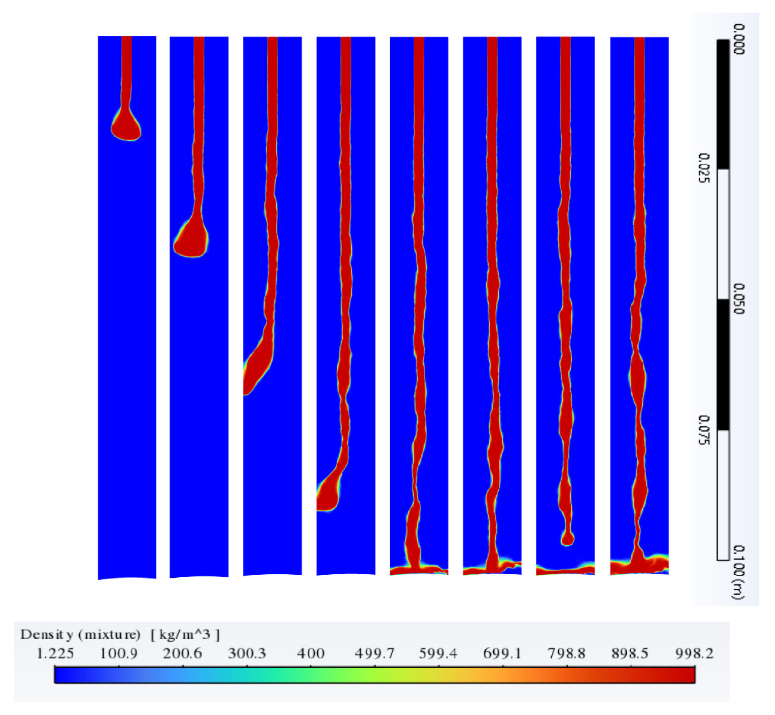
The simulation of the jet directed normally toward the grinding wheel, as shown in Figure 10, illustrates the onset of jet disintegration due to interaction with the crossflow generated by the rotating wheel. The length of the jet before breakup is shortened compared to the free planar jet (compare Figure 10 to Figure 8).

Figure 10. Development and breakup of planar jet impinging into rotating grinding wheel with the translational speed of its surface $U_g$ = 10U, where U = 1.5 m/s is velocity of jet. Snapshots are taken at consequent time moments with the time step Δt determined by ${\displaystyle \frac{U\Delta t}{L_D}} = 0.25$, where $L_D =0.1045 \mathrm{m}$ (55D) is the length of domain.

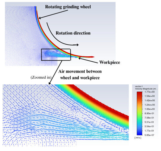
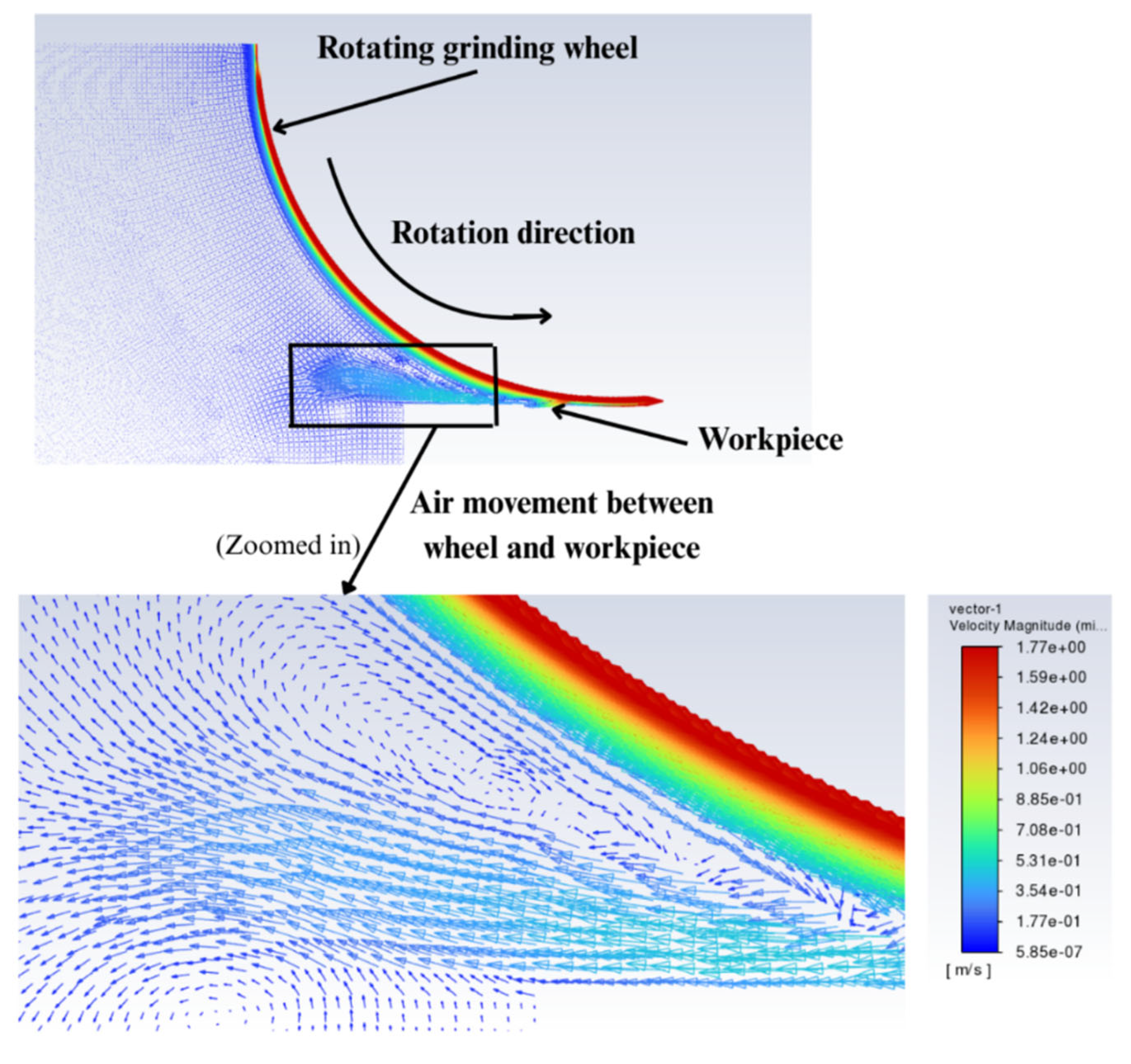
As another limit case, coolant jet is applied nearly parallel to the workpiece surface, a setup previously described by Ebbrell [41]. In this configuration, the presence of the workpiece restricts air movement near the wheel due to the narrow passage between the wheel and the workpiece (see Figure 11). This confinement may obstruct and divert the coolant flow, reducing its ability to reach the grinding zone effectively. Simulations based on this configuration were performed, and results are presented that illustrate how high-speed wheel rotation influences heat transfer.

Figure 11. Air layer around the rotating grinding wheel and workpiece.

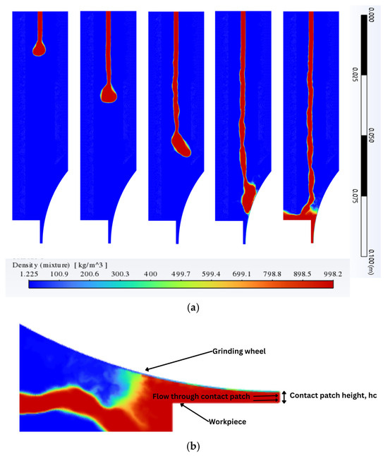
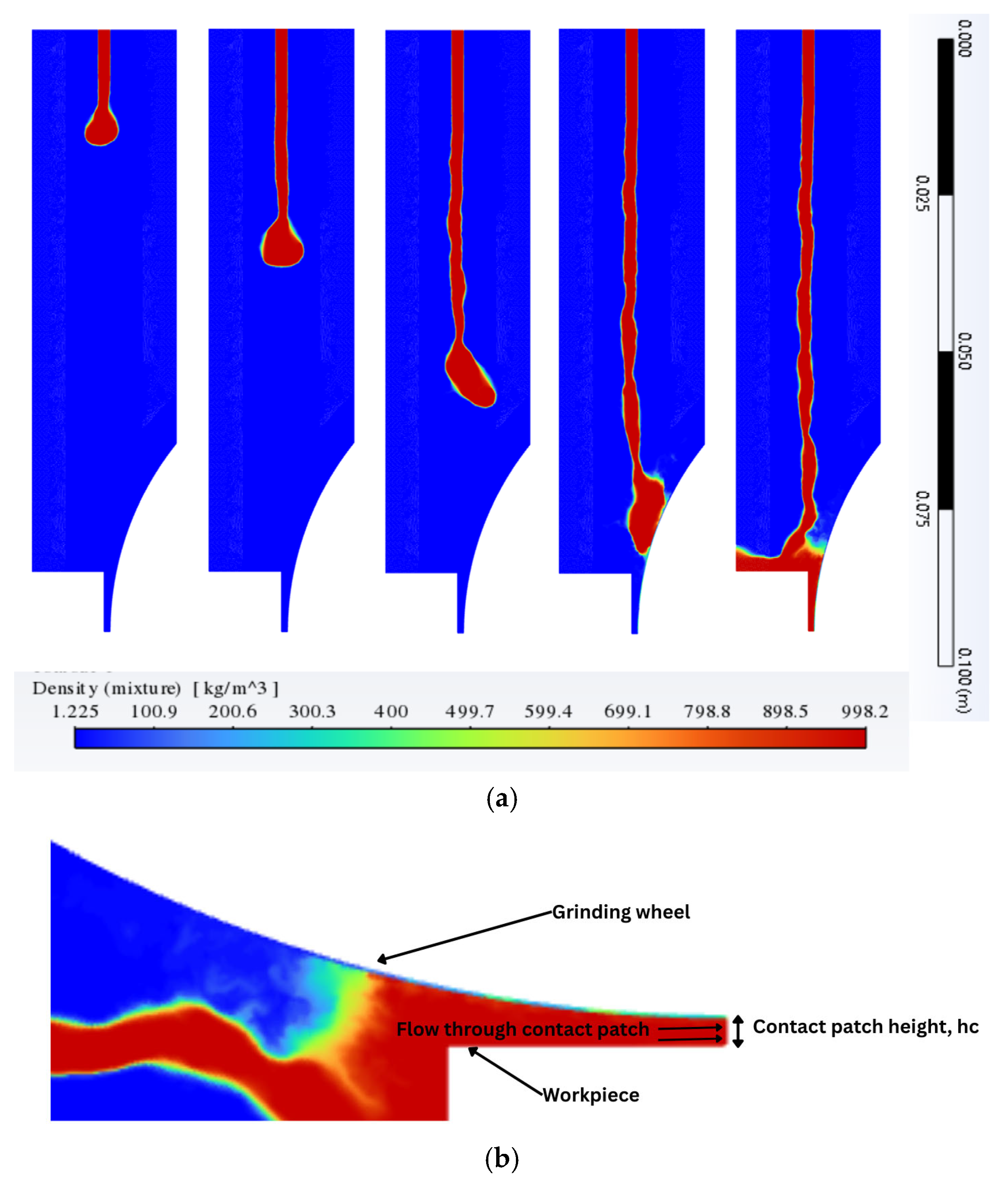
As shown in Figure 8, the complete breakup of the planar liquid jet occurs at 0.1045 m (55D) from the inlet. In a simulation where the same planar jet with identical average axial velocity, is directed tangentially toward a rotating grinding wheel and a nearby workpiece, the workpiece is positioned at 0.095 m (50D) from the inlet (Figure 1b), and the wheel center is located at 0.1045 m (55D). Under these conditions, the simulation results (Figure 12) showed that the jet breakup length remains comparable to that observed in the absence of the grinding wheel, indicating that the presence of the wheel and workpiece at these distances does not significantly affect the jet’s breakup behavior.

Figure 12. Development and breakup of planar jet with U = 1.5 m/s directed tangentially toward rotating grinding wheel with linear speed of its surface $U_g$ = 10 U with workpiece: (a) snapshots are taken at consequent time moments with the time step Δt determined by ${\displaystyle \frac{U\Delta t}{L_D}} = 0.25$, where $L_D =0.1045 \mathrm{m}$ (55D) is the length of domain; and (b) flow through the contact patch (enlarged view of last snapshot of sub-figure (a)).

The last frame in Figure 12a shows that part of the impinging liquid jet moves away from the rotating wheel (see enlarged view in Figure 12b), due to the air layer. This effect of jet moving slightly away from the wheel due to wheel rotation and surrounding air layer can cause reduction in the heat transfer from wheel to jet. Also, it can cause a reduction in coolant flow through the wheel-workpiece interface. This type of jet movement away from wheel can be affected by the wheel rotation speed depending on the distance of grinding wheel from the nozzle. The farther the jet travels, the more prone it is to break up or deflect due to outside disturbances like the wheel rotation.

Grinding wheels often lose their circularity over time because of intensive use, and a small gap can develop immediately after a layer of the workpiece material is removed. These effects lead to the formation of a momentary opening between the wheel and the workpiece, through which coolant can flow. This flow is captured and analyzed using the computational model. For coolant jet applications on grinding machines, the term “useful flow” (Smith and Curtis [42]) refers to the amount of coolant that passes through the contact patch between the grinding wheel and the workpiece (see Figure 12b). This parameter can be used as a measure of performance for a coolant jet. In most cases, more useful coolant flow is desirable. In this study, the developed computational model is used to perform a comparative analysis of ‘useful flow’ at two different wheel locations by calculating the coolant flow rate through the contact patch, characterized by a gap height $h_c$ = 0.95 mm.

When the wheel is set up at a closer distance to nozzle compared to that presented in Figure 12, the coolant flow through the contact patch is computed and presented in Table 4. It was observed that putting a shorter distance increases the jet’s ability to impinge in a better way that increases the useful flow by 25%.

Table 4. Flow rate through wheel-workpiece contact patch for 2D Cartesian jet in presence of grinding wheel, where D = 0.0019 m, contact patch height = 0.00095 m, $\mathrm{a}\mathrm{n}\mathrm{d} U_j$ = 1.5 m/s.

Wheel Distance from the Nozzle	$\mathbf{Non-Dimensional} \mathbf{Volume} \mathbf{Flow} \left(\frac{\mathit{V}\mathit{o}\mathit{l}\mathit{u}\mathit{m}\mathit{e}}{\mathit{\rho } \times {\mathit{U}}_{\mathit{j}} \times {\mathit{h}}_{\mathit{c}}}\right)$ Through Contact Patch per Unit of Width
55D	0.527
25D	0.703

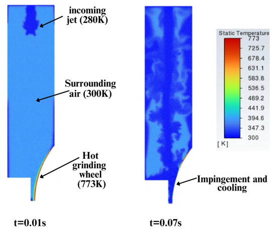
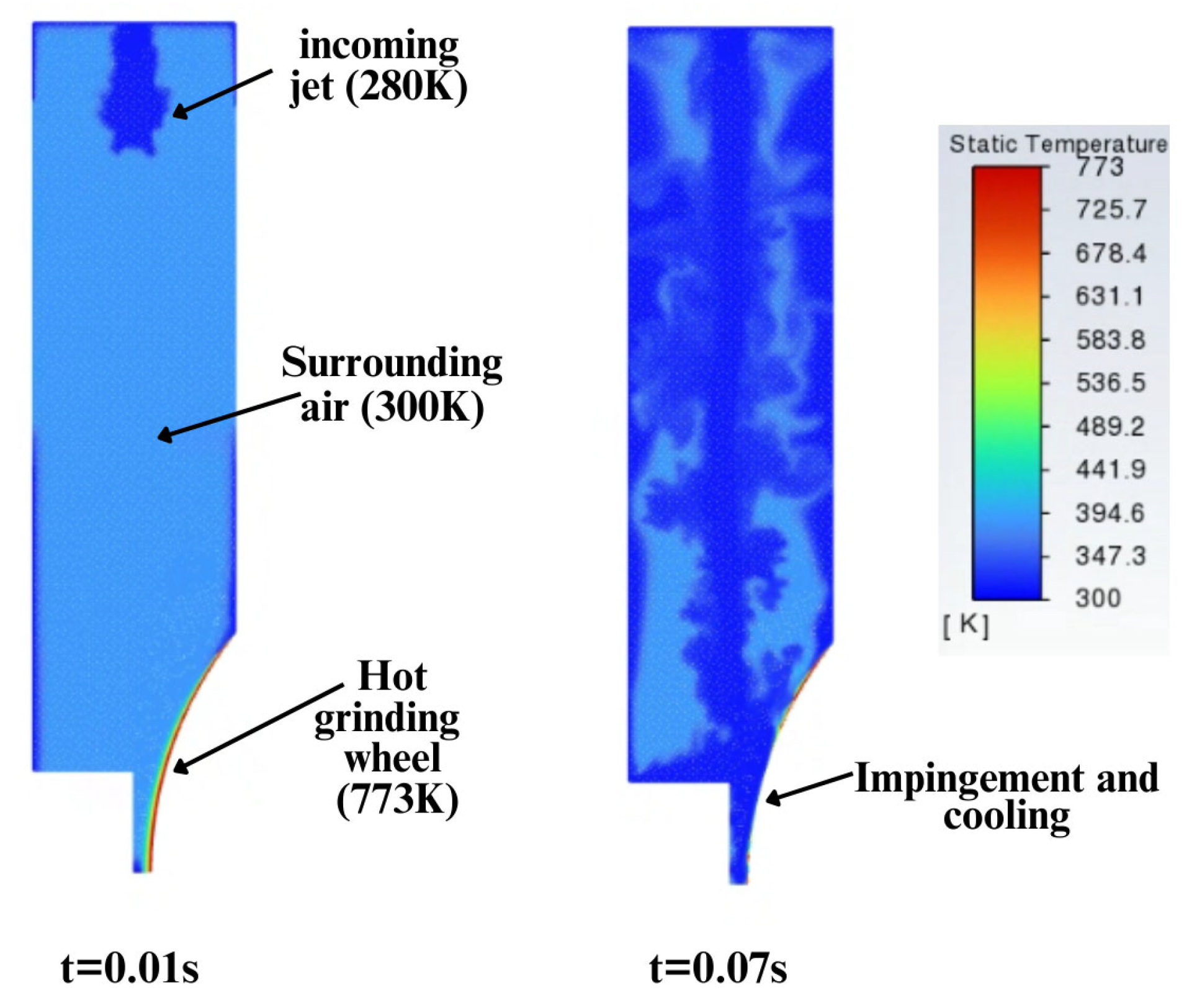
Next, the temperature field is analyzed to assess the cooling effect on the grinding wheel under tangential impingement of the coolant jet. The energy equation is activated for this set of simulations. The goal of numerical modeling in this section is to show how the jet’s cooling capabilities are affected by the rotational speed of the wheel. As the focus of this study is on the coolant jet modeling, the thermal setup is kept simplified, where the wheel has a temperature of 773K specified on its surface based on the findings by Pombo et al. [43], where they discuss the maximum temperature on grinding wheels ranging at 600K–1000K. The ambient air is initially set to have a temperature of 300K. After the coolant jet of 280K impinges on the wheel, Fluent calculates the cooling rate of wheel (see Table 5) through the wheel surface (specified as domain boundary) driven by convection introduced by coolant jet. The surface of grinding wheel was modeled as a no slip and no penetrating wall whereas porous nature of grinding wheel surface will be accounted for in future research. More detailed modeling of cooling the wheel will require thermophysical properties of wheel material to be specified. Figure 13 shows the temperature contours during the jet’s development and impingement on the wheel.

Table 5. Effect of air layer on heat transfer from wheel to coolant jet and surroundings.

Jet Velocity, Uj	Wheel Linear Velocity, Ug	Heat Transfer (W)
1.5 m/s	Uj	300,000
1.5 m/s	5Uj	235,000
1.5 m/s	10Uj	190,000

Figure 13. Contours of temperature before impingement (t = 0.01) and during impingement (t = 0.07 s).

The heat transfer from the wheel was obtained for three different relative ratios of wheel velocity to jet velocity, U_g/U_j. Previous studies have focused on determining the optimal grinding wheel speed relative to the incoming coolant jet. Webster [2] and Rowe [44] suggested that to reduce the strength of air layer for the jet to penetrate through it to the wheel, the jet bulk velocity should either match or exceed the wheel velocity. This suggestion has been widely adopted in industry and followed in the selection of wheel speed being equal to the jet speed in previously shown Table 4.

Upon increasing the wheel velocity U_g from U_g = U_j to larger values, U_g = 5U_j and U_g = 10U_j, the results in Table 5 indicate a reduction in the heat transfer rate. This decrease is attributed to decreasing the impact of jet impingement on the wheel surface, caused by the high-speed air layer due to faster wheel rotation.

This result indicates that an increasing speed of wheel disturbs the heat carrying capabilities of the coolant jet, which is the primary focus of this study.

One of the goals of present study is to explore coolant application techniques that require long distance jets due to lack of accessibility to grind zones, especially in inner diameter (ID) grinding. Prior studies [38,39] studied coolant jets located much closer to the wheel compared to the present study. This explains the lack of validation data for this part of the analysis.

The simplified 2D geometry considered for the jet–wheel interaction does not account for the finite width of a rectangular nozzle or the 3D edge effects associated with a finite-width grinding wheel. In addition, under the current setup, a uniform heat transfer distribution along the wheel width is assumed. This study will be extended to 3D modeling in future work, using the present results as a precursor. The findings reported here are therefore limited to qualitative assessment of the effect of wheel rotation speed on coolant jet performance.

3.6. Round Jets from Rouse Nozzle

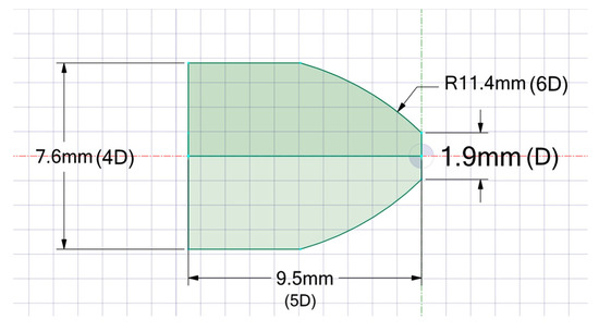
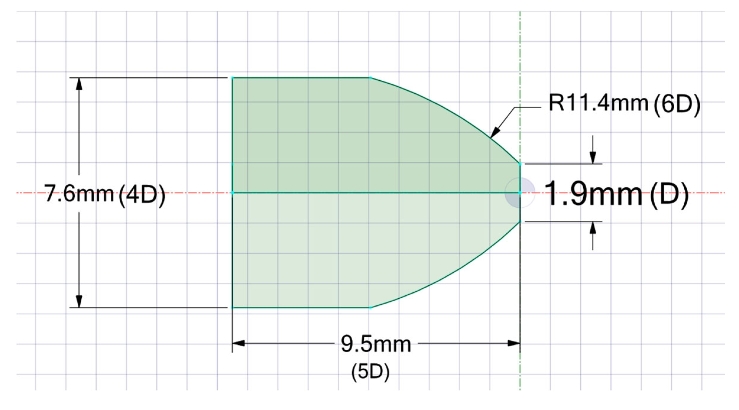
In this section, a computational domain that includes the nozzle was used to simulate the breakup of round jets issued from a nozzle with concave inner walls, commonly referred to as a Rouse nozzle [45], as shown in Figure 14. The Rouse [45] nozzle design used by Morgan et al. [46] was developed to reduce jet dispersion in liquid jets and extend the coherent or unbroken length of the liquid jet.

Figure 14. Schematic diagram of Rouse [45] with nozzle dimensions used in presented simulations.

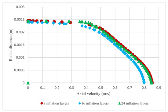
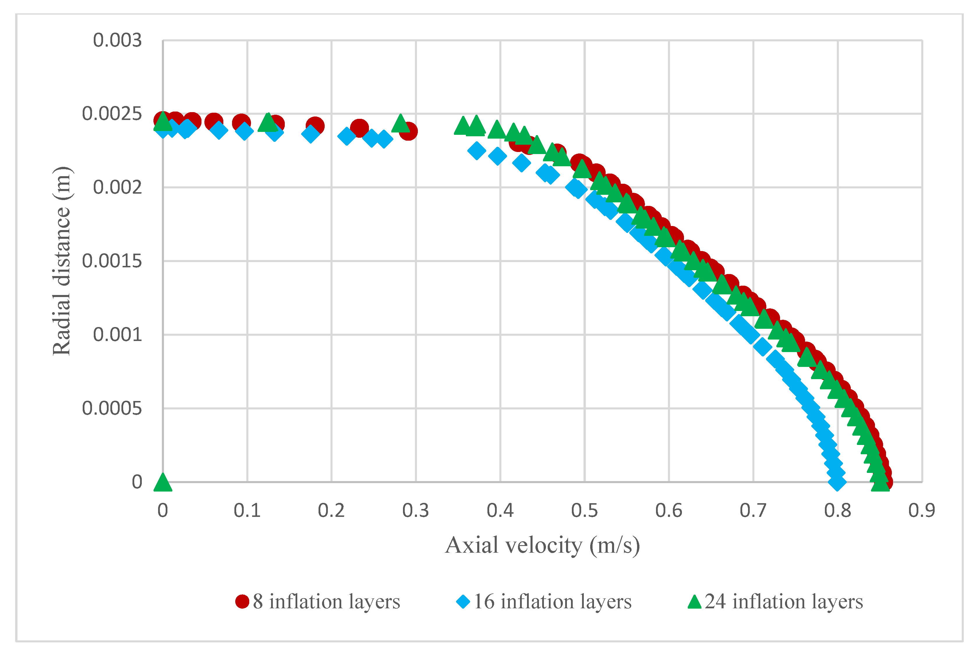
The developed numerical methodology discussed in Section 2 was applied to the domain incorporating the Rouse nozzle where the coolant flow from inside the nozzle is modeled. For results obtained in Section 3.3, the jet was modeled from the nozzle exit downstream, which excluded the nozzle geometry from the domain. Here the same FVM grids were used as shown in Figure 2a with the only exception being the presence of inflation layers on the no-slip nozzle walls. The smooth transition inflation option was chosen to generate the inflation layer grid where the transition ratio is defined that controls the jump of grid size from regular grid to inflation grid (0.272 is used in present case). The growth rate of the inflation layer is specified as equal to 1.35. Number of inflation grid layers determines the size of grid cells near the nozzle’s wall. Grid inflation with 8, 16 and 24 layers were generated to ensure the grid independence inside the nozzle. This is confirmed by results shown in Figure 15, where the developed velocity profile using different inflation layers is presented.

Figure 15. Developed velocity profiles at location upstream of the exit of the Rouse nozzle [45] for three different grid inflation layers.

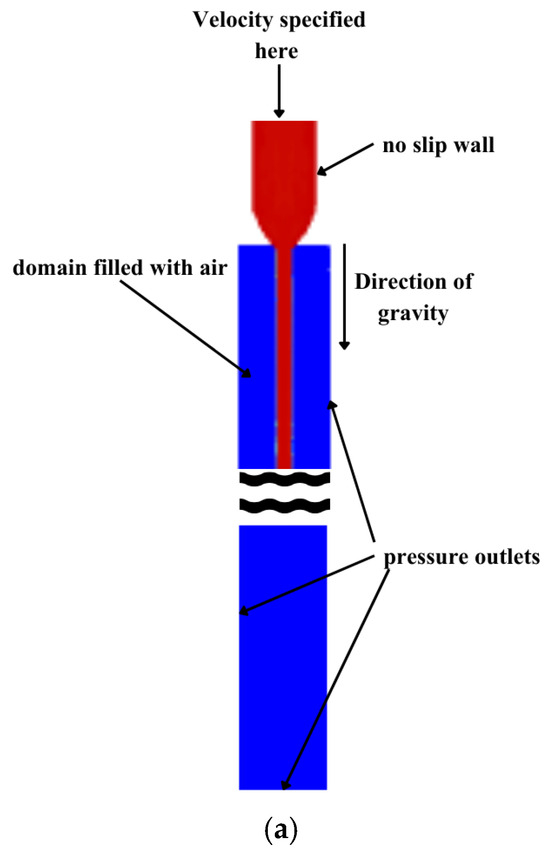
In the current setup with jet issuing by the Rouse nozzle, a uniform velocity profile is set at entrance location upstream of the converging section (x = −0.0095 m) (see Figure 14 and Figure 16a). In previous simulations without the nozzle, the non-uniform velocity profile was specified at jet inlet boundary, see Equation (4). In the considered case, the non-uniform velocity profile is developed as the coolant flow moves forward over the nozzle walls, bound by the no-slip boundary condition. The cross-sectional velocity profiles in Figure 15 show reasonable similarity to conclude that the flow inside the nozzle was resolved and does not depend on the number of inflation layers selected. The cross-section is taken at x = −1.9 mm, that is, at the distance of 1D upstream of the nozzle exit.

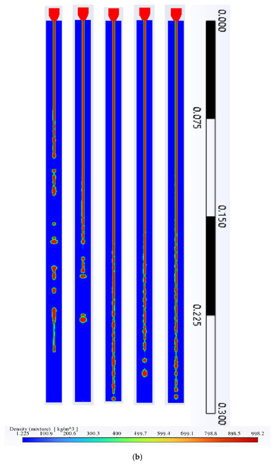
Figure 16. Modeling the jet produced by Rouse nozzle: (a) modified domain with inclusion of Rouse [45] nozzle and (b) disintegration of round liquid jet produced by Rouse nozzle with bulk velocity U = 3.89 m/s. Snapshots of jet breakup are taken at consequent moments with the time step Δt determined by ${\displaystyle \frac{U\Delta t}{L_D}}$ = 0.25, where L_D = 0.285 m (150D) is the length of domain.

Three different turbulent intensities were specified at the nozzle inlet to evaluate their effect on breakup length. The results obtained are presented in Table 6 and show that the inlet turbulence intensity has minor influence on the breakup length.

Table 6. Breakup lengths for different turbulent intensity at Rouse nozzle inlet.

Turbulent Intensity (%)	${\mathit{L}}_{\mathit{b}}/\mathit{D}$ for We = 400
5%	126
6.5%	123
7.5%	124

The authors also investigated a different nozzle, which has a straight channel instead of a Rouse nozzle [45] (see Table 7). The resulting jet breakup lengths were the same as the case where the nozzle geometry is excluded. Therefore, the discussed breakup of round jets in Section 3.3 was technically similar to a round jet issuing from a straight channel nozzle, which was used in prior experiments [23].

Table 7. Breakup lengths for different nozzles.

	$\mathbf{Normalized} \mathbf{Breakup} \mathbf{Length}, {\mathit{L}}_{\mathit{b}}/\mathit{D}$
Type of Nozzle	We = 235	We = 400
With Rouse [43] nozzle	89	126
Without nozzle (axisymmetric opening)	71	107

Figure 16 illustrates the development and breakup of a jet issued from a Rouse nozzle. It was observed that the jet from the Rouse nozzle exhibited a longer breakup length of 125D (1.125 m), compared to 107D for the regular round jet discussed in Section 3.3, for the same We number (We = 400). Both simulations used identical grid resolution. The increased breakup length demonstrates the effectiveness of the Rouse [45] design in comparison with a nozzle that has a constant radius.

Table 7 shows that, when the jet is modeled without nozzle to be coming out of an opening as inlet rather than a nozzle inside the domain, the observed breakup length is shorter. Therefore, Rouse [45] nozzle’s ability to increase jet coherence/breakup length is confirmed by the presented model.

4. Conclusions

A multiphase numerical model has been developed to simulate liquid jet breakup in simplified yet relevant domains representative of cooling in grinding technology, including the presence of a rotating grinding wheel near the workpiece. The 2D SST k-ω turbulence model was selected as a tradeoff between capturing the physics of jet breakup and needed computational resources based on a comparison of simulation results with previous experiments and simulations using various Reynolds-Averaged Navier–Stokes (RANS) models.

The following key quantitative and qualitative results were obtained by using the developed numerical model:

• Jets with a We number less than or equal to 400 exhibit Rayleigh-type instabilities, and the breakup length associated with these instabilities increases with jet speed proportional to √We.
• Rectangular jets disintegrate differently from round jets, displaying more turbulent structures.
• The decrease in wheel distance from nozzle increases the coolant flow through the gap between workpiece and wheel.
• An increase in wheel speed results in reduced heat transfer by the coolant from the grinding wheel.
• The use of Rouse nozzle increases the jet breakup length by 18% to 25% depending on the We number of the jet.

Building on this model, a 3D simulation framework will enable the study of jet breakup over a broader range of jet velocities and grinding conditions. The authors plan to develop a coolant delivery technique that extends the breakup length of the jet. Upgrading to a 3D domain will also allow for the resolution of nonlinear instabilities that are not fully captured in the current model.

References

- Eggers, J.; Villermaux, E. Physics of liquid jets. Rep. Prog. Phys. 2008, 71, 036601. [Google Scholar] [CrossRef] [Scilit]
- Webster, J.A.; Cui, C.; Mindek, R.B.; Lindsay, R. Grinding Fluid Application System Design. CIRP Ann. 1995, 44, 333–338. [Google Scholar] [CrossRef] [Scilit]
- Rupe, J.H. On the Dynamic Characteristics of Free-Liquid Jets and a Partial Correlation with Orifice Geometry; Jet Propulsion Laboratory, California Institute of Technology: Pasadena, CA, USA, 1962. Available online: https://ntrs.nasa.gov/citations/19620000813 (accessed on 15 January 2026).
- Debler, W.; Yu, D. The Break-up of Laminar Liquid Jets. Proc. R. Soc. Lond. Math. Phys. Sci. 1988, 415, 107–119. [Google Scholar] [CrossRef] [Scilit]
- Lefebvre, A.H.; McDonell, V.G. Atomization and Sprays; CRC Press: Boca Raton, FL, USA, 2017; p. 300. [Google Scholar] [CrossRef] [Scilit]
- Liu, H. Science and Engineering of Droplets: Fundamentals and Applications; William Andrew Publishing: New York, NY, USA, 1999. [Google Scholar] [CrossRef] [Scilit]
- Grant, R.P.; Middleman, S. Newtonian Jet Stability. AIChE J. 1966, 12, 669–678. [Google Scholar] [CrossRef] [Scilit]
- Lin, S.P.; Reitz, R.D. Drop and Spray Formation from a Liquid Jet. Annu. Rev. Fluid Mech. 1998, 30, 85–105. [Google Scholar] [CrossRef] [Scilit]
- McCarthy, M.J.; Molloy, N.A. Review of stability of liquid jets and the influence of nozzle design. Chem. Eng. J. 1974, 7, 1–20. [Google Scholar] [CrossRef] [Scilit]
- Goldstein, M.E.; Leib, S.J. The Role of Instability Waves in Predicting Jet Noise. J. Fluid Mech. 2005, 525, 37–72. [Google Scholar] [CrossRef] [Scilit]
- Huang, J.K.; Zhao, X. Numerical Simulations of Atomization and Evaporation in Liquid Jet Flows. Int. J. Multiph. Flow 2019, 119, 180–193. [Google Scholar] [CrossRef] [Scilit]
- Morad, M.R.; Nasiri, M.; Amini, G. Axis-Switching and Breakup of Rectangular Liquid Jets. Int. J. Multiph. Flow 2020, 126, 103242. [Google Scholar] [CrossRef] [Scilit]
- Pan, Y.; Suga, K. A Numerical Study on the Breakup Process of Laminar Liquid Jets into a Gas. Phys. Fluids 2006, 18, 052101. [Google Scholar] [CrossRef] [Scilit]
- Sakib, S.A.; Povitsky, A. Liquid coolant jet breakup with application to grinding; AIAA 2024-85879. In Proceedings of the 2024 Regional Student Conferences; American Institute of Aeronautics and Astronautics, Inc.: Reston, VA, USA, 2024; p. 85879. [Google Scholar] [CrossRef] [Scilit]
- Srinivasan, V.; Salazar, A.J.; Saito, K. Numerical investigation on the disintegration of round turbulent liquid jets using LES/VOF techniques. At. Sprays 2008, 18, 571–617. [Google Scholar] [CrossRef] [Scilit]
- Xiao, F.; Dianat, M.; McGuirk, J.J. LES of Turbulent Liquid Jet Primary Breakup in Turbulent Coaxial Air Flow. Int. J. Multiph. Flow 2014, 60, 103–118. [Google Scholar] [CrossRef] [Scilit]
- Pope, S.B. An explanation of the turbulent round-jet/plane-jet anomaly. AIAA J. 1978, 16, 279–281. [Google Scholar] [CrossRef] [Scilit]
- Yoder, D.A.; DeBonis, J.R.; Georgiadis, N.J. Modeling of Turbulent Free Shear Flows. Comput. Fluids 2015, 117, 212–232. [Google Scholar] [CrossRef] [Scilit]
- Ghahremanian, S.; Moshfegh, B. Evaluation of RANS Models in Predicting Low Reynolds, Free, Turbulent Round Jet. J. Fluids Eng. 2014, 136, 011201. [Google Scholar] [CrossRef] [Scilit]
- Zhao, J.F.; Yan, C.L.; Wu, L.Y.; Lin, W.; Tong, Y.H.; Nie, W.S. Numerical Simulation of Single/Double Liquid Jets in Supersonic Crossflows. Aerosp. Sci. Technol. 2022, 120, 107289. [Google Scholar] [CrossRef] [Scilit]
- Osher, S.; Fedkiw, R.; Piechor, K. Level set methods and dynamic implicit surfaces. Appl. Mech. Rev. 2004, 57, B15. [Google Scholar] [CrossRef] [Scilit]
- Osher, S.; Sethian, J.A. Fronts Propagating with Curvature-Dependent Speed—Algorithms Based on Hamilton–Jacobi Formulations. J. Comput. Phys. 1988, 79, 12–49. [Google Scholar] [CrossRef] [Scilit]
- Sallam, K.A.; Dai, Z.; Faeth, G.M. Liquid Breakup at the Surface of Turbulent Round Liquid Jets in Still Gases. Int. J. Multiph. Flow 2002, 28, 427–449. [Google Scholar] [CrossRef] [Scilit]
- Rayleigh, L. On the instability of jets. Proc. Lond. Math. Soc. 1878, 1, 4–13. [Google Scholar] [CrossRef] [Scilit]
- Kashiwa, B.A.; Rauenzahn, R.M. A Multimaterial Formalism; Tech. Rep. LA-UR-94-771; Los Alamos National Laboratory: Los Alamos, NM, USA, 1994. Available online: https://www.osti.gov/servlets/purl/10139551 (accessed on 15 January 2026).
- Eymard, R.; Gallouët, T.; Herbin, R.; Gutnic, M.; Hilhorst, D. Approximation by the Finite Volume Method of an Elliptic-Parabolic Equation Arising in Environmental Studies. Math. Model. Meth. Appl. Sci. 2001, 11, 1505–1528. [Google Scholar] [CrossRef] [Scilit]
- Anderson, D.; Tannehill, J.C.; Pletcher, R.H.; Munipalli, R.; Shankar, V. Computational Fluid Mechanics and Heat Transfer, 3rd ed.; CRC Press: Boca Raton, FL, USA, 2020. [Google Scholar] [CrossRef] [Scilit]
- Noh, W.F.; Woodward, P. SLIC (simple line interface calculation). In Proceedings of the Fifth International Conference on Numerical Methods in Fluid Dynamics, Enschede, The Netherlands, 28 June–2 July 1976; Springer: Berlin/Heidelberg, Germany, 2005; pp. 330–340. [Google Scholar] [CrossRef] [Scilit]
- Nichols, B.; Hirt, C. Methods for calculating multidimensional, transient free surface flows past bodies. In Proceedings of the 1st International Conference on Ship Hydrodynamics; Naval Ship Research and Development Center: Bethesda, MD, USA, 1975; pp. 253–277. [Google Scholar]
- DeBar, R.B. Fundamentals of the KRAKEN Code. [Eulerian Hydrodynamics Code for Compressible Nonviscous Flow of Several Fluids in Two-Dimensional (Axially Symmetric) Region]; Lawrence Livermore National Lab. (LLNL): Livermore, CA, USA, 1974. [Google Scholar] [CrossRef] [Scilit]
- Rusche, H. Computational Fluid Dynamics of Dispersed Two-Phase Flow at High Phase Fractions. Ph.D. Thesis, University of London, London, UK, 2002. Available online: https://cir.nii.ac.jp/crid/1573668924794647296 (accessed on 15 January 2026).
- Olsson, E.; Kreiss, G.; Zahedi, S. A Conservative Level Set Method for Two-Phase Flow II. J. Comput. Phys. 2007, 225, 785–807. [Google Scholar] [CrossRef] [Scilit]
- Menter, F.R. Two-Equation Eddy-Viscosity Turbulence Models for Engineering Applications. AIAA J. 1994, 32, 1598–1605. [Google Scholar] [CrossRef] [Scilit]
- Leonard, B.P.; Mokhtari, S. ULTRA-SHARP Nonoscillatory Convection Schemes for High-Speed Steady Multidimensional Flow; NASA Technical Memorandum NASA-TM-102568; NASA: Washington, DC, USA, 1990. Available online: https://ntrs.nasa.gov/citations/19900012254 (accessed on 15 January 2026).
- Ansys Fluent Manual. Choosing the Pressure Interpolation Scheme. Available online: https://ansyshelp.ansys.com/account/secured?returnurl=/Views/Secured/corp/v251/en/flu_th/flu_th_sec_solver_pb_mom_eq.html?q=presto (accessed on 15 January 2026).
- Pearson, K. On the criterion that a given system of deviations from the probable, in the case of a correlated system of variables, is such that it can be reasonably supposed to have arisen from random sampling. Philos. Mag. 1900, 50, 157–175. [Google Scholar] [CrossRef] [Scilit]
- Fisher, R.A.; Yates, F. Statistical Tables for Biological, Agricultural and Medical Research; Hafner Publishing Company: New York, NY, USA, 1953. [Google Scholar]
- Majumdar, S.; Banerjee, A.; Das, S.; Chakroborty, S. Experimental investigation and modelling on air layer formation around a rotating grinding wheel. Cogent Eng. 2016, 3, 1183273. [Google Scholar] [CrossRef] [Scilit]
- Lopez-Arraiza, A.; Castillo, G.; Dhakal, H.N.; Alberdi, R. High Performance Composite Nozzle for the Improvement of Cooling in Grinding Machine Tools. Compos. Part B Eng. 2013, 54, 313–318. [Google Scholar] [CrossRef] [Scilit]
- Baumgart, C.; Radziwill, J.J.; Kuster, F.; Wegener, K. A Study of the Interaction between Coolant Jet Nozzle Flow and the Airflow around a Grinding Wheel in Cylindrical Grinding. Procedia CIRP 2017, 58, 517–522. [Google Scholar] [CrossRef] [Scilit]
- Ebbrell, S.; Woolley, N.H.; Tridimas, Y.D.; Allanson, D.R.; Rowe, W.B. The Effects of Cutting Fluid Application Methods on the Grinding Process. Int. J. Mach. Tools Manuf. 2000, 40, 209–223. [Google Scholar] [CrossRef] [Scilit]
- Smith, E.D.; Curtis, D. An investigation of additively manufactured coolant nozzles for cylindrical grinding applications and progression to high stock removal. Procedia CIRP 2021, 101, 162–165. [Google Scholar] [CrossRef] [Scilit]
- Pombo, I.; Sánchez, J.A.; Martin, E.; Godino, L.; Álvarez, J. Accurate Measurement of Temperatures in Industrial Grinding Operations with Steep Gradients. Sensors 2024, 24, 1741. [Google Scholar] [CrossRef] [Scilit]
- Rowe, W.B. Principles of Modern Grinding Technology; William Andrew: Oxford, UK, 2013. [Google Scholar]
- Rouse, H.; Howe, J.W.; Metzler, D.E. Experimental investigation of fire monitors and nozzles. Trans. Am. Soc. Civ. Eng. 1952, 117, 1147–1175. [Google Scholar] [CrossRef] [Scilit]
- Morgan, M.N.; Baines-Jones, V. On the coherent length of fluid nozzles in grinding. Key Eng. Mater. 2009, 404, 61–67. [Google Scholar] [CrossRef] [Scilit]
Disclaimer/Publisher’s Note: The statements, opinions and data contained in all publications are solely those of the individual author(s) and contributor(s) and not of MDPI and/or the editor(s). MDPI and/or the editor(s) disclaim responsibility for any injury to people or property resulting from any ideas, methods, instructions or products referred to in the content. |
© 2026 by the authors. Licensee MDPI, Basel, Switzerland. This article is an open access article distributed under the terms and conditions of the Creative Commons Attribution (CC BY) license.