


Abstract
Monitoring the operating status of energy storage power stations can detect battery faults in enough time to prevent them from evolving into serious accidents capable of causing economic losses or even casualties. In this paper, a novel data-driven operating status monitoring method named dynamic local preserving projection–local outlier factor (DLPP-LOF) is proposed to improve the system safety performance of energy storage power stations. First, considering that the data collected by the battery management system of the energy storage power station have temporal correlations, the collected data are augmented so that the constructed augmentation matrix can effectively contain the autocorrelation in the data. Then, based on the local preserving projection (LPP) method, manifold features are effectively extracted from the augmented data matrix to preserve the meaningful local structure. Because the data in the battery management system of the energy storage power station do not display any specific distribution, it is not possible to perform traditional T2 and SPE statistical analysis. Therefore, we propose the use of the local outlier factor (LOF) method to obtain statistics from monitoring for early warning relating to fault status. Finally, the effectiveness and superiority of the proposed DLPP-LOF method are illustrated by applying it to a practical energy storage power station and comparing the results with those of classical methods.
1. Introduction
Solar and wind power are used to generate electricity and cannot always keep up with the demands of peak electricity consumption. As such, the use of renewable energy has long been plagued by energy storage problems. The key to unlocking the potential of renewable energy lies in energy storage power stations. In recent years, because of the improvement in the performance of energy storage technology, the reduction in costs, the prominent contradiction between the supply and demand of the power grid, and the introduction of incentive policies, the economy of battery energy storage technologies with long lives, low costs, and high energy conversion efficiencies has gradually become prominent. The application of energy storage technology is gradually shifting from project demonstration to commercial operation.
As a new energy battery, lithium-ion batteries are not only environmentally friendly but also have superior performance qualities and are widely used in energy storage power stations. However, lithium-ion battery technology itself has a safety problem that cannot be ignored. Because of thermal runaway caused by fire, explosions, and other accidents—inevitably causing property losses and casualties—lithium-ion battery safety issues are also gaining more and more attention. Hence, the energy storage battery has a high degree of nonlinearity, is temperature-sensitive, and shows obvious aging characteristics and inconsistencies, resulting in the thermal runaway of the battery pack because of its own chemical reaction heat release accumulation or the influence of external heat sources, seriously affecting the safety performance of the energy storage power station.
The development of safer and more effective energy storage power stations imposes higher requirements regarding the health status monitoring and fault warning of key pieces of equipment in energy storage power stations. In energy storage power station systems, hundreds of lithium-ion battery cells constitute a very complex system. Because of the larger capacity of the current energy storage power station, the higher voltage level of the grid, the limited capacity of the battery energy storage unit composed of the energy storage battery, and the bidirectional converter, the collector system is required to connect to the battery energy storage unit to form a complete energy storage power station, and the safety performance of the corresponding system faces a great test. This has higher requirements in terms of the health status monitoring and fault warning of energy storage power stations. Status monitoring and fault detection of the battery in the energy storage power station are completed through the battery management system, which is responsible for data collection, real-time status monitoring, and fault analysis of the energy storage battery pack.
According to a review article published by Venkatsubramanian et al. [1], status monitoring and fault detection methods can be divided into three categories according to different modeling methods: a knowledge-based approach, a mechanism model-based approach, and a data-driven approach. These methods have been extensively researched and developed over the past few decades and have gradually formed a mature framework. Knowledge-based methods are suitable for situations where a large amount of expert experience knowledge is available, and the generality of such methods is limited. In contrast, the method based on an analytic model is highly dependent on the mechanism employed and also requires higher abstraction and greater derivation of the mathematical model. As complexity increases, it becomes more difficult to obtain the corresponding mathematical model [2]. Because of the bottleneck in terms of acquiring expert knowledge and the difficulty in establishing accurate mathematical models, the above two methods have certain limitations when dealing with energy storage power station monitoring [3]. The data-driven method uses the collected process data to build a model, extract features, mine hidden information, and judge the running state of the energy storage power station. Compared with the knowledge-based and analytic model-based methods, the data-driven method is simple in terms of modeling, has a low demand in terms of establishing accurate mathematical models, is less dependent on expert knowledge, and can mine information from massive amounts of data. Therefore, research into data-driven status monitoring and fault detection has been given more and more attention [4,5,6,7].
As a typical data-driven method, multivariate statistical analysis is one of the most widely used methods. Its core idea is to model the correlation between process variables through a feature extraction algorithm and construct corresponding monitoring statistics to monitor the operating status and conduct fault detection [8,9,10]. Commonly used multivariate statistical analysis methods include principal component analysis (PCA) [11,12,13,14], canonical correlation analysis, canonical correlation analysis (CCA) [15,16,17], projection on latent structure (PLS) [18,19,20], slow feature analysis (SFA) [21,22], and so on. PCA projects the original data into a new coordinate system by means of a linear transformation, making the projected variables independent of each other. For state monitoring and fault detection, PCA aggregates data from multiple variables into several principal components and then constructs statistics using the feature vectors obtained from dimensionality reduction [23]. Compared with PCA, PLS is widely used to extract the advantages of potential variables by establishing the relationship between input and output space [24]. However, PLS decomposition is a slant decomposition, which still contains components orthogonal to performance indicators in the relevant space. To solve this problem, Zhou [25] proposed a total projection to latent structures (TPLS). Through further decomposition in the main space and residual space, the fine-grained monitoring based on four data subspaces was realized. He et al. [26] pointed out that using global methods such as PCA and PLS for dimensional reduction would lead to the destruction of the local structure of data.
In order to solve the problem that dimensionality reduction destroys the local structure of data, a manifold learning algorithm is introduced into the field of state monitoring and fault detection. Unlike other multivariate statistical analysis methods, manifold learning algorithms usually include steps to find data neighborhoods, that is, to determine the nearest neighbor points or all the nearest neighbors within the radius of each sample based on some index [27,28,29]. In addition, the optimization function of manifold learning algorithms usually takes the integrity of the local neighborhood structure as the main objective or constraint. Typical methods include locality preserving projections (LPP) [30], locally linear embedding (LLE) [31,32], neighborhood preserving embedding (NPE) [33,34,35], and so on. Different from the global model, the above algorithm based on manifold learning considers the local structure information of the data and can effectively extract the local information of data by maintaining the local geometry structure of the data in the process of dimensionality reduction. Manifold learning algorithms can be divided into linear and nonlinear methods, wherein the nonlinear algorithm does not involve the calculation of the projection matrix in the conversion process from the original space to the feature space, while the linear algorithm can obtain the projection matrix. When the manifold learning algorithm is applied to online operating state monitoring and fault detection, new samples need to be projected into the feature space of the training data.
In order to improve the system safety performance of energy storage power stations, the dynamic local preserving projection–local outlier factor method is proposed in this paper. Based on the battery parameter data collected by the battery management system, a big data-driven energy storage power station operation status monitoring and fault detection model is built to give early warning of the fault status of the energy storage power station and ensure the safe, high-quality, and economic operation of the entire energy storage power station. Firstly, since the collected data have dynamic temporal correlation, the augmentation method is used to expand the dataset so that the constructed augmentation matrix can effectively contain the autocorrelation in the data. Secondly, the manifold features are extracted from the augmented matrix obtained in the previous step based on the local preserving projection method, which can preserve the local structure. Third, given that the complex characteristics of the battery management system data of the energy storage power station do not meet any distributions, the state monitoring statistics are constructed based on the local outlier factor. Finally, the proposed method is applied to an actual energy storage power station, and the effectiveness and superiority of the method are demonstrated. The novelty of our work in this manuscript includes the following:
- (1)
- The dynamic local preserving projection–local outlier factor method is proposed to improve the system safety performance of energy storage power stations.
- (2)
- The augmentation method is used to expand the dataset so that the constructed augmentation matrix can effectively contain the autocorrelation of the data.
- (3)
- The manifold features are extracted from the augmented matrix to preserve the meaningful local structure.
2. The Proposed DLPP-LOF Method
2.1. Dynamic Data Augment Strategy of the Energy Storage Power Station
In the proposed DLPP-LOF method, the normal dataset collected from the battery management system is converted into an augmented data matrix to consider the temporal correlation in the data from the energy storage power station. The specific augmentation process is as follows:
The dataset matrix collected by the battery management system under the normal operation of the energy storage power station is , where is the number of samples and is the number of variables. The dynamic delay is set to ; its value is generally 1 or 2, and it is used to indicate the order of the dynamic system of the energy storage power station [36].
samples are used before the current time to stack the current time samples. Therefore, the original data matrix augments to become a novel data matrix , where the dimension of each augmented sample is .
2.2. Local Feature Extraction Through LPP
LPP is a typical feature extraction method for manifold learning [37]. Compared with the method of preserving the global structure, the LPP method extracts the local manifold features and is more robust and less sensitive to noise in the dataset. In the mechanism of LPP, the local structure maintenance is implemented by distance invariance. In other words, in the original data space, the distance between data is the same as that in the feature space after dimensionality reduction. In the original space, after obtaining the distance matrix between the data, the features in the low-dimensional feature space are recovered by keeping the distance matrix unchanged. Based on the LPP algorithm, the local manifold structure of the dataset can be extracted effectively. By obtaining a projection matrix that maintains the local structure of the dataset, the augmented high-dimensional data matrix of the energy storage power station can be transformed into a low-dimensional feature data matrix . The detailed local feature extraction process is listed as follows.
(1) Construct the neighbor connection diagram: According to the distance, samples close to sample in are selected as its neighbors. The commonly used distances are Euclidean distance, Mahalanobis distance, and so on. If data is one of the K neighbors of data , a straight line is connected between node and node . Otherwise, node and node are not connected. Through this step, the neighbor connection graph can be constructed so that each sample in is connected to its neighbors and not connected to points that are not its neighbors.
(2) Weight calculation in the neighbor connection graph: Let be the weight matrix in the neighbor connection graph to be found, and represent the weight value between node and node . If there is no connection between node and node in the neighbor connection diagram, the value is set to zero. If there is a line between node and node in the neighbor connection graph, the value is set using the Gaussian kernel function as follows:
where is a Gaussian kernel parameter.
(3) Eigen mapping matrix calculation [38]: According to the weight matrix obtained in the previous step, the projection matrix can be obtained by taking the eigenvector of the following formula:
Once the projection matrix is obtained, the low-dimensional manifold eigenvector of the energy storage power station dataset can be represented as follows:
As a result, the low-dimensional manifold of the energy storage power station dataset can be obtained through .
2.3. Monitoring Statistics Construction and Control Limit Estimation
Given that the data of the battery management system of the energy storage power station does not meet any distribution, the accuracy of the state monitoring model will be greatly reduced if the traditional T2 and SPE statistics are constructed. Therefore, the local outlier factor method is proposed to construct monitoring statistics for the early warning of fault status. The local outlier factor was originally proposed to find outliers in the dataset. Compared with the normal dataset, the fault data have a large outlier degree [37,39]. The value of the LOF indicates the degree to which the data point is an outlier. For the low-dimensional manifold of the energy storage power station, the LOF monitoring statistic is constructed according to the following steps:
(1) Neighborhood construction: For the low-dimensional manifold of the energy storage power station ( is the number of samples in , is the number of dimensionalities in ), the Euclidean distance between each data point and the remaining data is calculated and then sorted from nearest to farthest. Each data point selects its nearest data as its nearest neighbors to form the neighborhood. is the nearest neighbor of , and is the Euclidean distance between data and its neighbor .
(2) calculation: The neighborhood of data point is established as according to the previous step. The radius of this neighborhood is set as . That is, the is equal to the Euclidean distance between the data point and its farthest neighbor in the neighborhood .
(3) Reachability distance calculation [39]: The reachability distance between the data point in the low-dimensional manifold of the energy storage power station and its nearest neighbor is defined as follows:
According to the above formula, the reachability distance is the larger value between and . Using the reachability distance can reduce statistical fluctuations. For the same neighborhood, the smaller the number of neighbors, the greater the reachability distance difference. The larger the number of neighbors, the more similar the reachability distance.
(4) Local reachability density calculation [39]: The local reachability density of the data point in the low-dimensional manifold of the energy storage power station is defined as follows:
In the above formula, the local reachability density of the data point in the low-dimensional manifold of the energy storage power station represents the average reachability distance between the data point and its neighbors in the neighborhood .
(5) Local outlier factor calculation [39]: The local outlier factor of the data point in the low-dimensional manifold of the energy storage power station is defined as follows:
According to the defined reachability distance and the defined local reachability density , the outlier degree of the data point in the low-dimensional manifold of the energy storage power station is determined by its neighborhood . Compared with traditional statistics T2 and SPE, the statistics based on LOF do not need to satisfy the assumption that the data obey a specific distribution and can use higher-order information.
The calculation of LOF is based on the density information. If the density of the data point in the low-dimensional manifold of the energy storage power station is similar to the density of other data in its neighborhood , the resulting LOF value is close to 1. If the density of the data point in the low-dimensional manifold of the energy storage power station is different from the density of other data in the neighborhood , the resulting LOF value is much greater than 1. Therefore, the control limit of LOF can be determined as 1. In addition, in order to estimate the control limit more accurately, the kernel density estimation method is used to determine the control limit.
In the stage of the online monitoring and fault detection of the energy storage power station, the low-dimensional manifold characterization of the online testing data is obtained. Then, for , the nearest neighbor is found in the low-dimensional manifold of the energy storage power station, and its LOF value is calculated. By comparing it with the control limit, the current operating state of the energy storage power station can be determined.
2.4. The Procedure of the DLPP-LOF Method
The offline modeling phase is as follows:
- (1)
- Obtain the training dataset of the energy storage power station .
- (2)
- Augment to become a novel data matrix containing the temporal correlation.
- (3)
- Standardize the augmented dataset according to the z-score method.
- (4)
- Employ the LPP method to extract features for , and obtain the projection matrix .
- (5)
- Establish the monitoring statistic for exacted features based on the LOF method.
- (6)
- Estimate the control limit of the monitoring statistic using the KDE method.
The online monitoring phase is as follows:
- (1)
- Obtain the testing data .
- (2)
- Augment to contain the temporal correlation as .
- (3)
- Standardize based on the mean and standard deviation of the .
- (4)
- Project the standardized using the feature space and acquire the feature .
- (5)
- Construct the LOF monitoring indicator of by searching the nearest neighbors in the low-dimensional manifold .
- (6)
- If the monitoring statistic of never exceeds the control limit, it is normal. If the monitoring statistic of exceeds the control limit, the fault occurs.
3. Case Study
3.1. Numerical Example
A numerical example is designed as follows:
A total of five variables containing y and u are selected as monitored variables. Then, 500 data points are collected under normal working conditions as a training dataset. Two testing datasets are set as follows:
Testing dataset 1: First, it runs under normal working conditions. From the 201st point, there is a fault: the D matrix becomes . A total of 1000 testing data points are collected.
Testing dataset 2: First, it runs under normal working conditions. From the 201st point, there is a fault: occurs at a step of 1.2. A total of 1000 testing data points are collected.
The proposed DLPP-LOF method is tested according to the numerical example above. To prove the effectiveness of DLPP-LOF, it is compared with the PCA method, which is widely used in process monitoring. Moreover, to prove the effectiveness of the DLPP method for feature extraction, the proposed DLPP-LOF method is compared with the direct use of LOF. This paper compares the performance of algorithms by the false alarm rate and the missed alarm rate. The false alarm rate refers to the proportion of normal data that is incorrectly judged to be fault data. The missed alarm rate refers to the proportion of fault data that is incorrectly judged to be normal.
For PCA, the feature space dimension is determined according to the variance contribution of 85%. In both LOF and DLPP-LOF methods, the number of is determined to be 10 according to the cross-validation method. In the DLPP-LOF method, the delay is determined to be 1, and the dimension of the DLPP-LOF method feature space is determined to be nine according to the cross-validation method.
Table 1 lists false detection rates in the energy storage power station, and Table 2 lists missed detection rates for the numerical example. As shown in these two tables, the false detection rates obtained by the three methods are all below 2%, which is satisfactory.
Table 1.
False detection rates in the numerical example.
Table 2.
Missed detection rates in the numerical example.
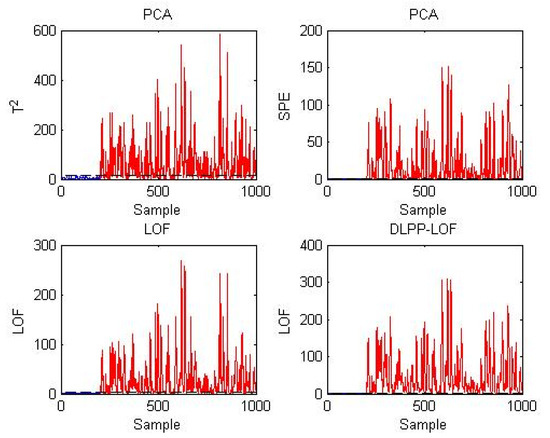
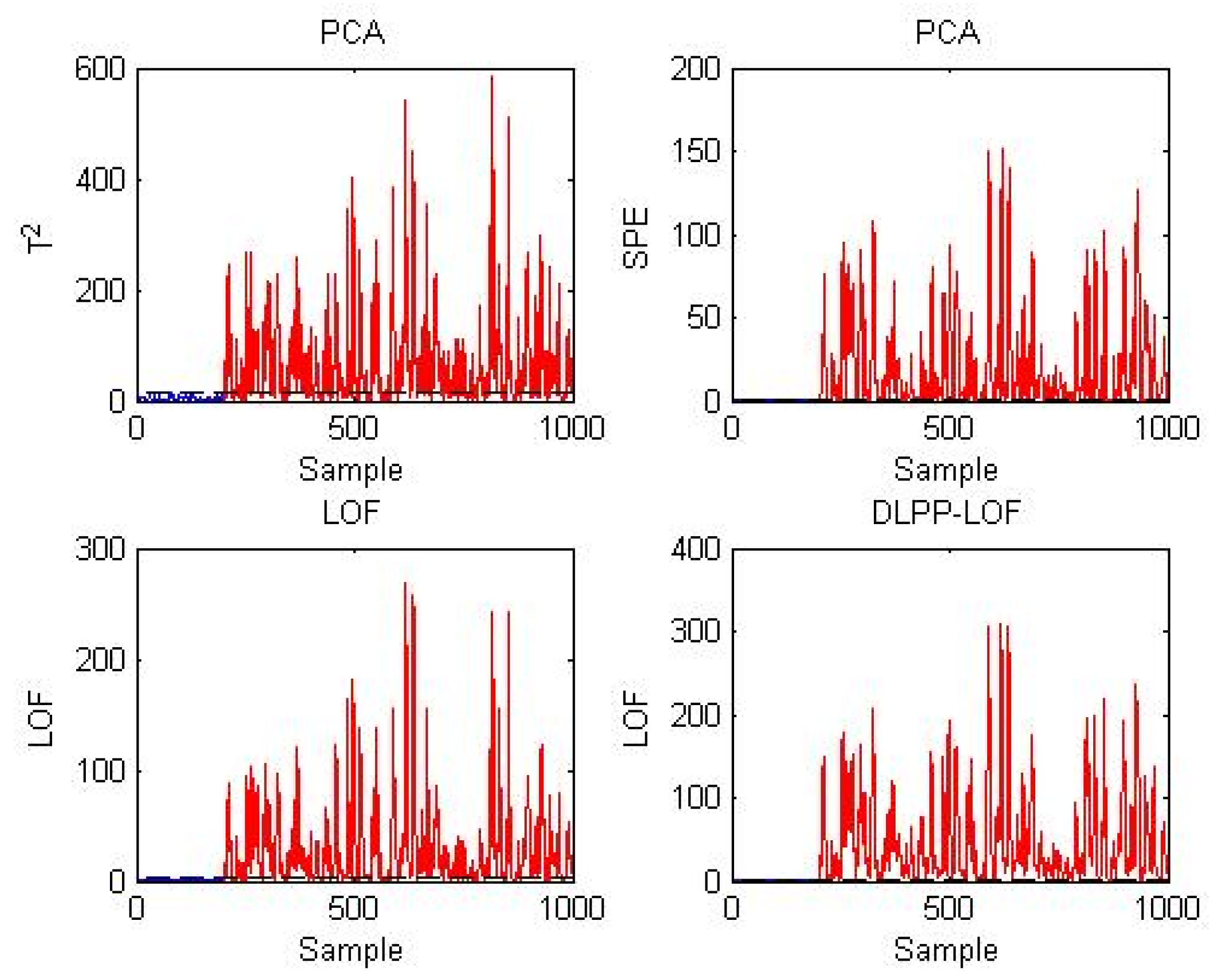
In testing dataset 1, the D matrix changes. The detection results of this testing dataset are shown in Figure 1. Based on this figure, the T2 and SPE statistics of PCA can judge almost 80% of the fault samples, and the missed detection rate is 21.125% and 21.5%, respectively. In contrast to PCA, the detection performance of the LOF method is reduced, and more than 60% of the fault samples are misjudged as normal samples. Among the PCA, LOF, and DLPP-LOF methods, the proposed DLPP-LOF method can detect this fault accurately, where the missed rate of DLPP-LOF is 3.75%. Compared with the LOF method, the better detection performance obtained by DLPP-LOF shows the effectiveness of feature extraction using DLPP.
Figure 1.
Results of three methods for testing dataset 1 of the numerical example.
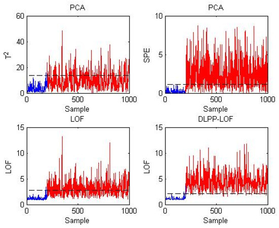
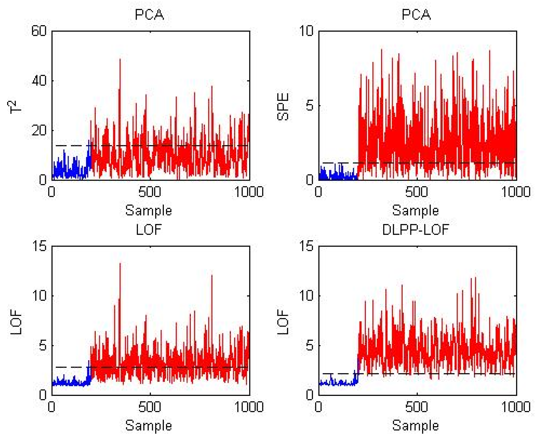
For testing dataset 2, occurs at a step of 1.2. Figure 2 shows the results of PCA, LOF, and DLPP-LOF on testing dataset 2. It can be seen in this figure that the T2 statistics of PCA almost cannot detect the occurrence of this step fault. Compared with the T2 statistics, the SPE statistics of PCA can detect faults, and 22.625% of the fault samples cannot be successfully detected. For the LOF method, 41.125% of the fault samples are wrongly judged as normal. Compared with the PCA method and LOF method, the DLPP-LOF method can achieve the best detection performance, where more than 95% of the fault samples are effectively detected, and the missed detection rate reaches 3.625%.
Figure 2.
Results of three methods for testing dataset 2 of the numerical example.
3.2. Energy Storage Power Station
The proposed DLPP-LOF method is tested and validated by analyzing the energy storage data collected from the Zhenjiang energy storage power station in China. In this energy storage power station, a battery cluster consists of 228 battery cells. In addition, voltage is an important feature of battery cells. Therefore, a total of 228 individual voltages are selected as monitoring variables, and 500 samples are collected as the training data. In order to demonstrate the effectiveness of the proposed method, it is compared with the PCA method, which is widely used in operation condition monitoring and fault detection. In addition, in order to demonstrate the effectiveness of the DLPP method for feature extraction, the proposed DLPP-LOF method is compared with the direct use of LOF for operating condition monitoring and fault detection.
In testing dataset 1, the first 100 samples are normal samples, and from point 101, the voltage of cell 168 occurs a step of 0.1.
In testing dataset 2, the first 100 samples are normal samples, and from point 101, the voltage of cell 140 experienced a slow drift fault with a slope of 0.001.
In the contrast algorithm PCA, the feature space dimension is determined according to the variance contribution of 85%. In both the LOF and DLPP-LOF methods, the number of is determined to be 10 according to the cross-validation method. In the DLPP-LOF method, the delay is determined to be 1, and the dimension of the DLPP-LOF method feature space is determined to be 120 according to the cross-validation method.
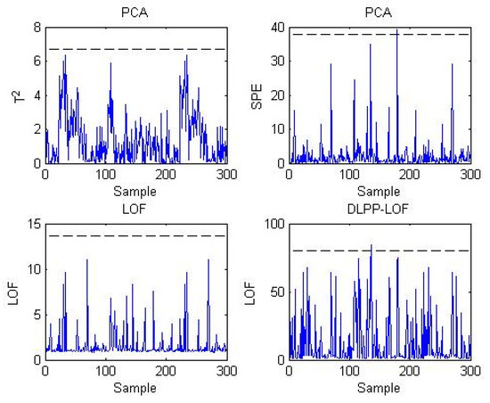
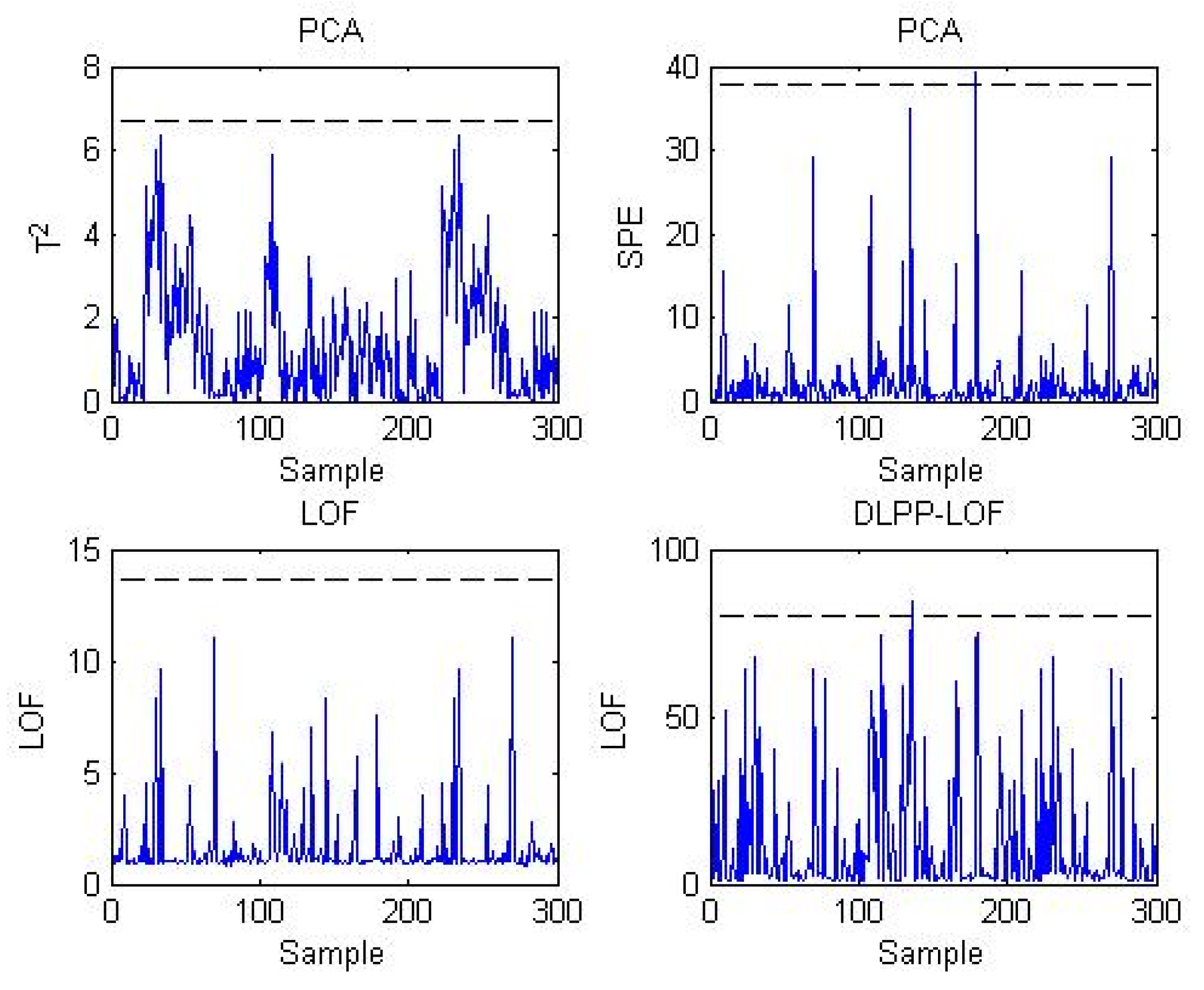
First, the testing results of three methods for the normal dataset are shown in Figure 3. As can be seen in Figure 3, the statistics of the three methods do not detect the fault. It can be shown that the detection performance of PCA, LOF, and DLPP-LOF is satisfactory for the normal process. Table 3 lists false detection rates in the energy storage power station, and Table 4 lists missed detection rates in the energy storage power station. As shown in these two tables, the proposed DLPP-LOF method can obtain the best false detection rates and missed detection rates in the energy storage power station.
Figure 3.
Testing results of three methods for the normal dataset.
Table 3.
False detection rates in the energy storage power station.
Table 4.
Missed detection rates in the energy storage power station.
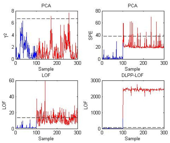
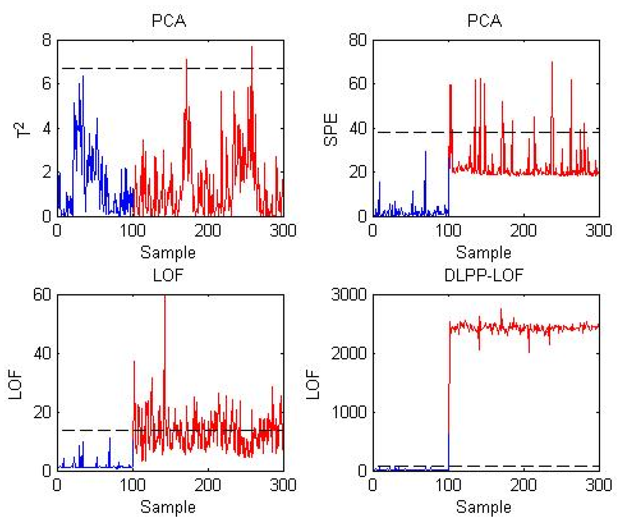
In testing dataset 1, the voltage of cell 168 occurs at a step of 0.1. The detection results of testing dataset 1 are shown in Figure 4. In this figure, the T2 statistics of PCA misjudge almost all the fault samples as normal samples, and the missing detection rate reaches 99%. Although the SPE statistic of PCA can detect the occurrence of this fault, the missed rate still exceeds 90%. Compared with PCA, the detection performance of the LOF method is improved, and less than 60% of the fault samples are misjudged as normal samples. Among the PCA, LOF, and DLPP-LOF methods, the proposed DLPP-LOF method can detect this fault accurately and identify each fault sample accurately, where the missed rate of DLPP-LOF is 0. The better detection performance shows the effectiveness of feature extraction using DLPP. This testing case shows that the proposed DLPP-LOF method has good detection performance for step faults.
Figure 4.
Results of the three methods for testing dataset 1 of the energy storage power station.
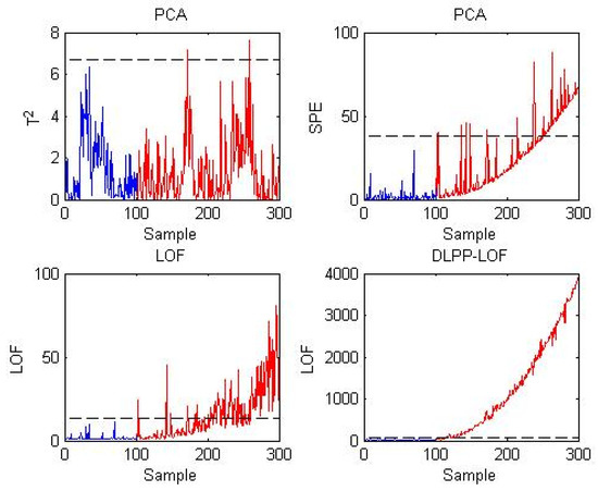
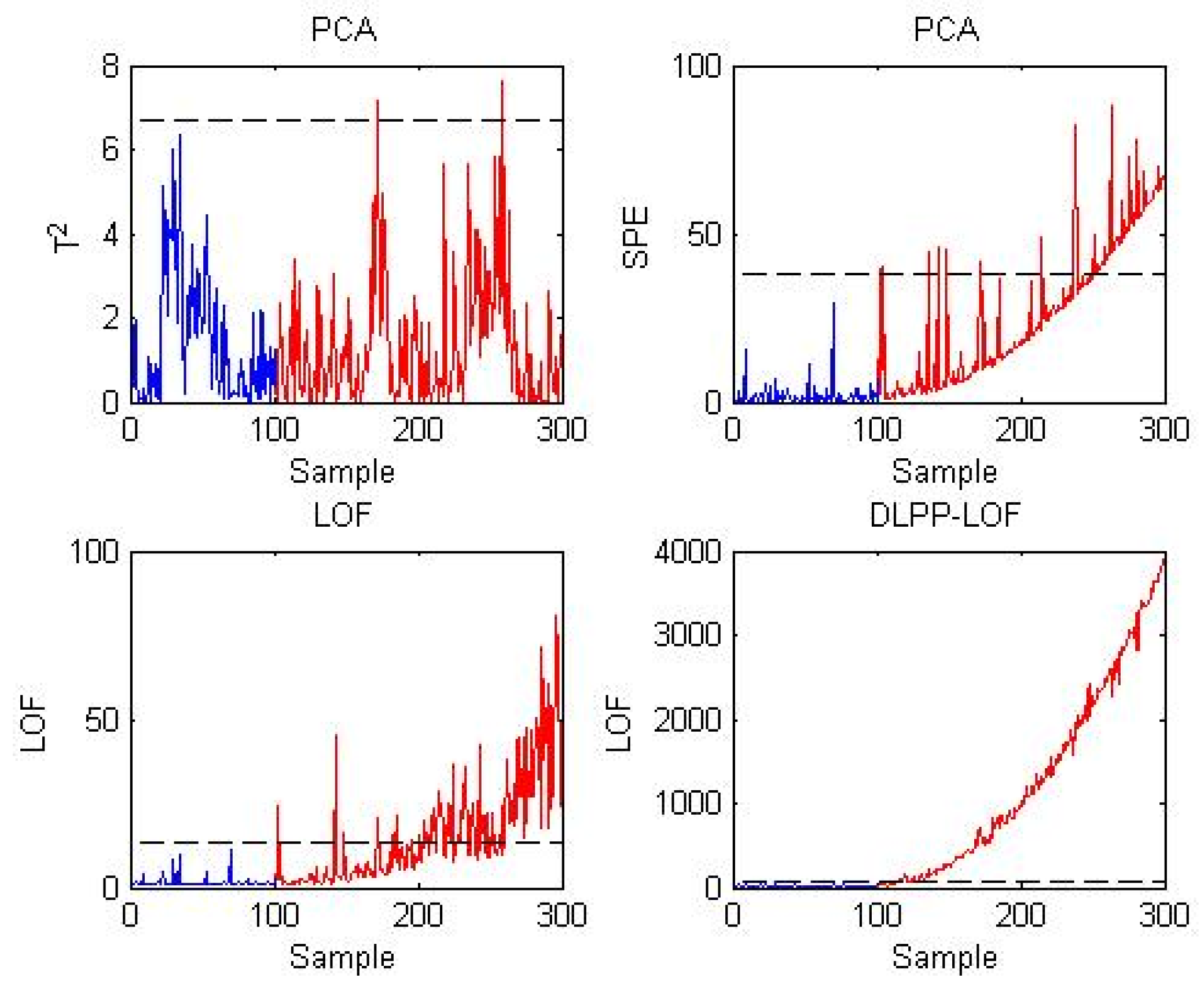
In testing dataset 2, the voltage of cell 140 experienced a slow drift fault with a slope of 0.001. Figure 5 shows the results of PCA, LOF, and DLPP-LOF on testing dataset 2. As can be seen in this figure, the T2 statistics of PCA cannot detect the occurrence of this drift fault. Compared with the T2 statistics, the SPE statistics of PCA can detect faults, and 29% of the fault samples are successfully detected. For the LOF method, 61.5% of the fault samples are wrongly judged as normal. Compared with the PCA method and the LOF method, the DLPP-LOF method can achieve the best detection performance, where more than 90% of the fault samples are effectively detected. This testing case shows that the proposed DLPP-LOF method has good detection performance for slow drift faults.
Figure 5.
Results of the three methods for testing dataset 2 of the energy storage power station.
4. Conclusions
In this paper, a novel DLPP-LOF method is proposed to monitor the operation state of energy storage power stations. In the DLPP-LOF method, considering the time correlation in data collected by the battery management system of the energy storage power station, the dynamic characteristics are included in the model by augmenting the data. Then, the LPP method, which can keep the low-dimensional manifold structure, is used to extract features from the augmented matrix. Finally, statistics are constructed based on the LOF method, and the control limit is determined by the KDE method. The proposed DLPP-LOF method is applied to a numerical example and an actual energy storage power station and compared with the PCA method and the LOF method. Based on the false alarm rate and missed alarm rate obtained in the numerical examples and practical applications, the proposed DLPP-LOF method can obtain the best monitoring results, which shows the effectiveness and superiority of the proposed method.
In future work, in order to establish a more accurate monitoring model of the operation state, unique detection methods for early faults of energy storage power stations can be developed. In addition, for different modes of energy storage power stations, monitoring models for multimode energy storage power stations can be established.
Author Contributions
Conceptualization, W.H.; methodology, W.H.; validation, L.C.; investigation, Z.L.; resources, Z.L.; data curation, J.L.; writing, J.L.; writing—review and editing, L.Z.; visualization, L.Z. Validation, B.S. All authors have read and agreed to the published version of the manuscript.
Funding
This work was supported by the Management Consulting Project of Taizhou Power Supply Company of State Grid Zhejiang Electric Power Co., Ltd. (SGZJTZ00YXJS2400333).
Data Availability Statement
Data are unavailable because of privacy concerns.
Conflicts of Interest
The authors declare that this study received funding from Taizhou Power Supply Company of State Grid Zhejiang Electric Power Co., Ltd. The funder was not involved in the study design, collection, analysis, interpretation of data, the writing of this article or the decision to submit it for publication.
References
- Venkatasubramanian, V.; Rengaswamy, R.; Yin, K.; Kavuri, S.N. A review of process fault detection and diagnosis: Part I: Quantitative model-based method. Comput. Chem. Eng. 2003, 27, 293–311. [Google Scholar]
- Magott, J.; Skrobanek, P. Timing analysis of safety properties using fault trees with time dependencies and timed state-charts. Reliab. Eng. Syst. Saf. 2012, 97, 14–26. [Google Scholar] [CrossRef] [Scilit]
- Gao, D.; Wu, C.G.; Zhang, B.K.; Ma, X. Signed Directed Graph and Qualitative Trend Analysis Based Fault Diagnosis in Chemical Industry. Chin. J. Chem. Eng. 2010, 18, 265–276. [Google Scholar] [CrossRef] [Scilit]
- Song, B.; Zheng, C.F.; Jin, Y.T.; Shi, H.B.; Tao, Y.; Tan, S. A Fault Targeted Gated Recurrent Unit-Canonical Correlation Analysis Method for Incipient Fault Detection. IEEE Trans. Ind. Inform. 2024, 20, 8739–8748. [Google Scholar] [CrossRef] [Scilit]
- Chen, J.W.; Song, P.Y.; Zhao, C.H. Multi-scale self-supervised representation learning with temporal alignment for multi-rate time series modeling. Pattern Recognit. 2024, 145, 109943. [Google Scholar] [CrossRef] [Scilit]
- Song, B.; Zhou, Y.C.; Shi, H.B.; Tan, S.; Tao, Y. A Soft Sensor for Multirate Quality Variables Based on MC-CNN. IEEE Trans. Neural Netw. Learn. Syst. 2024, 36, 13927–13938. [Google Scholar] [CrossRef] [Scilit] [PubMed]
- Liu, D.; Wang, Y.; Liu, C.; Yuan, X.; Yang, C. Multirate-former: An efficient transformer-based hierarchical network for multi-step prediction of multirate industrial processes. IEEE Trans. Instrum. Meas. 2023, 73, 2502313. [Google Scholar] [CrossRef] [Scilit]
- Wang, Y.; Wan, Y.; Zhang, H.; Yang, W. Robust decomposition of kernel function-based nonlinear robust multimode process monitoring. IEEE Trans. Instrum. Meas. 2023, 72, 3511711. [Google Scholar] [CrossRef] [Scilit]
- Cui, P.; Wang, X.; Yang, Y. Nonparametric manifold learning approach for improved process monitoring. Can. J. Chem. Eng. 2022, 100, 67–89. [Google Scholar] [CrossRef] [Scilit]
- Zhu, Q.; Liu, Q.; Qin, S.J. Concurrent quality and process monitoring canonical correlation analysis. J. Process Control 2017, 60, 95–103. [Google Scholar] [CrossRef] [Scilit]
- Lan, T.; Tong, C.D.; Shi, X.H. Variable weighted principal component analysis algorithm and its application in fault detection. J. Chem. Ind. Eng. 2017, 68, 3177–3182. [Google Scholar]
- Xiao, B.; Li, Y.; Sun, B.; Yang, C.; Huang, K.; Zhu, H. Decentralized PCA modeling based on relevance and redundancy variable selection and its application to large-scale dynamic process monitoring. Process Saf. Environ. Prot. 2021, 151, 85–100. [Google Scholar] [CrossRef] [Scilit]
- Song, B.; Shi, H.B. Fault Detection and Classification using Quality Supervised Double-Layer Method. IEEE Trans. Ind. Electron. 2018, 65, 8163–8172. [Google Scholar] [CrossRef] [Scilit]
- Zheng, D.; Zhou, L.; Song, Z. Kernel generalization of multi-rate probabilistic principal component analysis for fault detection in nonlinear process. IEEE/CAA J. Autom. Sin. 2021, 8, 1465–1476. [Google Scholar] [CrossRef] [Scilit]
- Chen, Z.; Zhang, K.; Ding, S.X.; Shardt, Y.A.; Hu, Z. Improved canonical correlation analysis-based fault detection methods for industrial processes. J. Process Control 2016, 41, 26–34. [Google Scholar] [CrossRef] [Scilit]
- Song, B.; Shi, H.; Tan, S.; Tao, Y. Multisubspace orthogonal canonical correlation analysis for quality-related plant-wide process monitoring. IEEE Trans. Ind. Inform. 2020, 17, 6368–6378. [Google Scholar] [CrossRef] [Scilit]
- Chen, Q.; Liu, Z.; Ma, X.; Wang, Y. Artificial neural correlation analysis for performance-indicator-related nonlinear process monitoring. IEEE Trans. Ind. Inform. 2021, 18, 1039–1049. [Google Scholar] [CrossRef] [Scilit]
- Peng, K.X.; Zhang, K.; Li, G. Quality-related process monitoring based on total kernel PLS model and its industrial application. Math. Probl. Eng. 2013, 2013, 707953. [Google Scholar] [CrossRef] [Scilit]
- Zheng, Y.; Liu, Z.W.; Yang, W.D.; Tao, B.; Wang, Y.W. Parallel projection to latent structures for quality-relevant process monitoring. J. Taiwan Inst. Chem. Eng. 2017, 80, 76–84. [Google Scholar] [CrossRef] [Scilit]
- Zhou, J.L.; Zhang, S.L.; Zhang, H.; Wang, J. A quality-related statistical process monitoring method based on global plus local projection to latent structures. Ind. Eng. Chem. Res. 2018, 57, 5323–5337. [Google Scholar] [CrossRef] [Scilit]
- Qin, Y.; Zhao, C.H. Comprehensive process decomposition for closed-loop process monitoring with quality-relevant slow feature analysis. J. Process Control 2019, 77, 141–154. [Google Scholar] [CrossRef] [Scilit]
- Zhao, C.; Huang, B. A full-condition monitoring method for nonstationary dynamic chemical processes with cointegration and slow feature analysis. AIChE J. 2018, 64, 1662–1681. [Google Scholar] [CrossRef] [Scilit]
- Tamura, M.; Tsujita, S. A study on the number of principal components and sensitivity of fault detection using PCA. Comput. Chem. Eng. 2007, 31, 1035–1046. [Google Scholar] [CrossRef] [Scilit]
- Yin, S.; Wang, G.; Gao, H. Data-driven process monitoring based on modified orthogonal projections to latent structures. IEEE Trans. Control Syst. Technol. 2015, 24, 1480–1487. [Google Scholar] [CrossRef] [Scilit]
- Zhou, D.; Li, G.; Qin, S.J. Total projection to latent structures for process monitoring. AIChE J. 2010, 56, 168–178. [Google Scholar] [CrossRef] [Scilit]
- He, F.; Xu, J. A novel process monitoring and fault detection approach based on statistics locality preserving projections. J. Process Control 2016, 37, 46–57. [Google Scholar] [CrossRef] [Scilit]
- Zhang, N.; Tian, Y.; Wang, X.W.; Xu, Y.; Zhu, Q.X.; He, Y.L. Novel bootstrap-based discriminant NPE integrated with orthogonal LPP for fault diagnosis. IEEE Trans. Instrum. Meas. 2023, 72, 3506309. [Google Scholar] [CrossRef] [Scilit]
- Chen, H.; Wu, J.; Jiang, B.; Chen, W. A modified neighborhood preserving embedding-based incipient fault detection with applications to small-scale cyber–physical systems. ISA Trans. 2020, 104, 175–183. [Google Scholar] [CrossRef] [Scilit] [PubMed]
- Wang, Y.; Liang, J.; Ling, D.; Gu, X.G.; Li, S. The chemical process monitoring method based on temporal extended orthogonal neighbourhood preserving embedding (TONPE). Can. J. Chem. Eng. 2023, 101, 1455–1468. [Google Scholar] [CrossRef] [Scilit]
- Luo, L.; Bao, S.; Mao, J.; Tang, D. Nonlocal and local structure preserving projection and its application to fault detection. Chemom. Intell. Lab. Syst. 2016, 157, 177–188. [Google Scholar] [CrossRef] [Scilit]
- Zhang, Y.; Fu, Y.; Wang, Z.; Feng, L. Fault detection based on modified kernel semi-supervised locally linear embedding. IEEE Access 2017, 6, 479–487. [Google Scholar] [CrossRef] [Scilit]
- Miao, A.; Song, Z.; Ge, Z.; Zhou, L.; Wen, Q. Nonlinear fault detection based on locally linear embedding. J. Control Theory Appl. 2013, 11, 615–622. [Google Scholar] [CrossRef] [Scilit]
- Miao, A.; Ge, Z.; Song, Z.; Shen, F. Nonlocal structure constrained neighborhood preserving embedding model and its application for fault detection. Chemom. Intell. Lab. Syst. 2015, 142, 184–196. [Google Scholar] [CrossRef] [Scilit]
- Song, B.; Song, Y.M.; Jin, Y.T.; Shi, H.B.; Tao, Y.; Tan, S. Plant-wide Process Fine-scale Monitoring via Distributed Static Magnitude-Dynamic Difference. IEEE Trans. Ind. Inform. 2023, 19, 10864–10872. [Google Scholar] [CrossRef] [Scilit]
- Song, B.; Ma, Y.; Shi, H.B. Multimode process monitoring using improved dynamic neighborhood preserving embedding. Chemom. Intell. Lab. Syst. 2014, 135, 17–30. [Google Scholar] [CrossRef] [Scilit]
- Ku, W.F.; Storer, R.H.; Georgakis, C. Disturbance detection and isolation by dynamic principal component analysis. Chemom. Intell. Lab. Syst. 1995, 30, 179–196. [Google Scholar] [CrossRef] [Scilit]
- Mu, L.X.; Sun, W.Z.; Zhang, Y.M.; Feng, N.; Xue, X.H.; Li, Q.L. A fault isolation strategy for industrial processes using outlier-degree-based variable contributions. ISA Trans. 2024, 152, 113–128. [Google Scholar] [CrossRef] [Scilit] [PubMed]
- Shah, M.Z.H.; Hu, L.; Ahmed, Z. Modified LPP based on Riemannian metric for feature extraction and fault detection. Measurement 2022, 193, 110923. [Google Scholar] [CrossRef] [Scilit]
- Qian, C.; He, N.; He, L.L.; Li, R.X.; Cheng, F. A weighted Gaussian process regression model based on improved local outlier factor and its application in state of health estimation of lithium-ion battery. Eng. Appl. Artif. Intell. 2024, 138, 109314. [Google Scholar] [CrossRef] [Scilit]

Disclaimer/Publisher’s Note: The statements, opinions and data contained in all publications are solely those of the individual author(s) and contributor(s) and not of MDPI and/or the editor(s). MDPI and/or the editor(s) disclaim responsibility for any injury to people or property resulting from any ideas, methods, instructions or products referred to in the content. |
© 2026 by the authors. Licensee MDPI, Basel, Switzerland. This article is an open access article distributed under the terms and conditions of the Creative Commons Attribution (CC BY) license.