


Abstract
Fiber–obstacle interactions are important in refining processes, where fibers interact with solid surfaces under shearing flow. In this study, a coupled CFD–DEM approach is used to investigate the effects of obstacle height, fiber flexibility, fiber length, and flow velocity on the flow field, fiber motion, and shear stress around an obstacle. The fluid flow is solved using OpenFOAM and fiber motion using LIGGGHTS, with fibers represented by bonded spherical particles. Three obstacle heights, h/H = 0.25, 0.50, and 0.75, are considered in a 1 mm high channel. Increasing the obstacle height promotes fiber accumulation and modifies the flow structure around the obstacle. The effect of fibers on obstacle shear stress depends strongly on obstacle height: compared with the fiber-free case, the averaged shear stress increases by approximately 68% for h/H = 0.25, changes by only 3% for h/H = 0.50, and decreases by approximately 31% for h/H = 0.75. The reduction at the highest obstacle may be attributed to the formation of a fiber layer that partially shields the obstacle from the main flow. Fiber flexibility and length further influence the balance between fiber–wall interaction, fiber–fiber interaction, and flow-induced forces. These results demonstrate that obstacle geometry and fiber properties jointly control momentum transfer and fiber accumulation around obstacles.
1. Introduction
The pulp and paper industry is a complex sector that requires the precise manipulation of fibrous materials in suspension through various stages of production to achieve the desired quality and properties of the final paper product. One critical stage in this process is low consistency refining, where the suspension enters at the center of a disk, flows between it and a parallel disk, and exits at the outer edge of the disks. One of the disks is stationary and the other is rotating. As fibers pass through the refiner, they encounter rotating and stationary bars that create intricate dynamics, impacting fiber length, fiber property distribution, and overall suspension homogeneity.
Understanding these interactions is essential for optimizing refining conditions to improve the efficiency and sustainability of the production process. Key factors such as refiner speed, gap clearance, and pulp consistency all contribute to shaping how these interactions affect the mechanical treatment and transport of fibers. These dynamics can influence important aspects of the production process, such as energy consumption, process efficiency, and the overall quality of the final paper.
Previous studies have provided significant insights into the forces acting on fibers during refining. According to Lumiainen [1], Nugroho [2], and Technology [3], there are two different forces acting on fibers during each bar crossing in a refiner: one is due to fiber–wall interaction, and the other originates from fiber–fiber interaction. Martinez and Kerekes [4] were among the first to attempt measuring the forces acting on fiber flocs between passing bars in a single-bar refiner. They observed that the range of gap sizes where the forces on the fibers were significant was narrow. Within this range, they identified two extremes: at the upper limit, flocs are compressed to almost zero void fraction, and at the lower limit, they are split into two. Martinez et al. [5] proposed an expression for the normal forces acting on an ideal floc during compression. They assumed that the flocs are spherical, unable to support significant normal load, and that compression happens in a linear elastic fashion. Their model agreed with data from pure compression experiments on nylon flocs. Similarly, Batchelor et al. [6] tried to model the shear forces acting on an ideal floc during bar passage in a refiner. Their resulting expression showed good agreement with experimental results from a single-bar refiner. Further research by Kerekes and Senger [7] aimed to characterize the refining action in low-consistency refiners by analyzing forces acting on fibers. They proposed correlations to quantify refining action based on fiber response to these forces, reporting that the force exerted on fibers is a function of the distribution of fibers in the gap or the bar coverage and the amount of fiber in the gap. Kerekes [8] emphasized that force, rather than energy, is responsible for variations in fiber properties, focusing on characterizing refining action based on force instead of energy. Kerekes [9] linked the forces on bars to the forces acting on fibers using the distribution of fibers over bars and gap size. The predicted forces on fiber mass and bars show a good agreement with experimental measurements in both high-consistency and low-consistency refiners for mechanical pulp.
An important parameter usually associated with the forces on fibers is the number of fibers trapped at the bars, or “stapled”. Lundin et al. [10] noted that refining does not occur unless fibers are trapped at the bar edges and reported that lower fiber trapping at reduced consistencies results in harsher refining conditions on the fibers at a given refining power. Batchelor et al. [11] found that the fraction of refiner bars that trap fibers is a function of fiber consistency. Based on experimental results, they concluded that the reduction in refining efficiency with decreasing pulp consistency is likely due to a decrease in the number of fibers trapped at the leading edge of the bars.
Recent research has focused on in-depth experimental observations and advanced modeling techniques to analyze the behavior of pulp fibers within refiners. Aigner et al. [12] expanded on previous experimental studies by employing a high-resolution rotary encoder and a piezo ceramic force sensor to examine the effect of the gap on the bar-force profile. The high-resolution rotary encoder allowed the researchers to determine the force distribution at various rotor positions relative to the stator during each bar-passing event. Jouybari et al. [13] conducted numerical simulations of softwood pulp flow in both rotating and non-rotating grooves, employing computational fluid dynamics (CFD) techniques. Using the OpenFOAM software (OpenFOAM-5.x), they studied the influence of factors such as consistency, gap thickness, angular velocity, and radial positions. Their findings indicated that shear forces increase linearly with angular velocity and can be modeled as Couette flow. Furthermore, they examined variations in the pressure coefficient using Bernoulli’s principle, emphasizing the predominant role of compression effects within the groove. This study aims to elucidate the interactions between fibers and walls, as well as fiber-to-fiber interactions in refiners, focusing on their relevance to the pulp and paper industry. By analyzing the critical factors affecting these interactions through numerical simulations using CFDEM, with the DEM part modeled in LIGGGHTS and the CFD part in OpenFOAM, this research intends to facilitate future studies, improving industry practices and understanding of fiber–bar interactions. This can lead to optimized refining processes, and higher quality products. The effects of different parameters such as the height of the obstacle in the channel, fiber stiffness, fiber velocity and fiber length on the forces acting on fibers and the tendency of fibers to get stapled at the obstacle edge are investigated.
2. Governing Equations
2.1. CFD
The turbulence effects are negligible for the lower Reynolds numbers considered in this study. Although increasing the velocity of the upper moving wall increases the Reynolds number to values at which turbulence could be expected in the corresponding single-phase flow, turbulence effects remain weak in the present fiber-laden system. The high concentration of fibers enhances energy dissipation through fiber–fiber collisions and fiber–fluid interactions, while simultaneously attenuating turbulent fluctuations and suppressing the development of large-scale eddies, as discussed by Brandt and Coletti [14]. The general form of continuity and Navier–Stokes equations are expressed as
where f denotes liquid, p is the index for solid, is the void fraction, i.e., the volume content of a calculation cell, is the fluid density, is the fluid velocity vector, is the solid velocity vector, p is the pressure, τ is the liquid stress tensor, is the implicit momentum exchange term between solid and liquid phases, g is the gravity vector and f is the explicit momentum exchange term from solid to the liquid phase. The in Equation (2) is calculated from the forces acting on the CFD field and the fiber forces through the momentum coupling model, as
where is the CFD cell volume.
The fluid-phase equations are solved in a filtered LES framework. In this framework, the velocity vector in Equation (2) represents the resolved (filtered) velocity, . The effects of the unresolved subgrid-scale motions are accounted for through an eddy viscosity, , which is added to the molecular kinematic viscosity, , to define the effective viscosity as = + . Accordingly, the viscous stress tensor in Equation (2) is evaluated using the effective viscosity, replacing with . The WALE model is used to determine the subgrid-scale eddy viscosity:
where
where are the components of the following deviatoric symmetric tensor:
where
In most cases, the modeled turbulent viscosity is small compared with the molecular viscosity, indicating that molecular momentum transport is dominant under the corresponding flow conditions. At the higher wall velocities, locally elevated values of , reaching the same order of magnitude as the molecular viscosity, are observed in limited regions of the flow. However, the time-averaged turbulent viscosity over the solution domain remains substantially smaller than the molecular viscosity, indicating that the overall contribution of the modeled subgrid-scale viscosity is limited.
2.2. DEM
The equations governing the particle i motions in rotational and translational modes are presented as
where is the contact forces acting on a particle, represents the bond forces, is the force exerted by the surrounding fluid phase and represents body forces acting on a particle. represents moments arising due to contact forces, is the bond moments acting on particles in a fiber and represents the external moments acting on fibers. Model A is used in the present study according to the classification presented in Zhou et al. [15], meaning that the pressure is shared between the two phases. The pressure gradient and viscous forces are taken into account in the force models in addition to the Koch–Hill drag model [16]. The Hertz contact model is used to calculate the forces in spheres after particle–particle and particle–wall interactions [17].
3. Geometry and Numerical Simulation
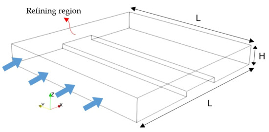
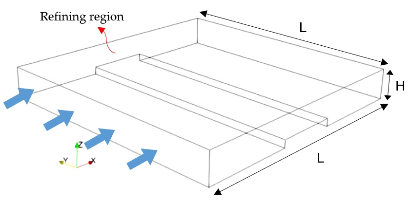
The study examines the geometry shown in Figure 1, where an obstacle is positioned at the center of the lower wall within a channel. The channel dimensions are H = 1 mm in height and L = 4 mm in length for the base case simulations. The arrows in Figure 1 illustrate the flow direction and highlight the refining region, which is the area between the upper plate and the top of the obstacle. The height of the obstacle, h, is varied to investigate its effects on the flow field within the channel and the forces acting on the particles. Additionally, the study explores the distribution of shear stress on both the channel walls and the obstacle under different conditions. The primary objectives are to understand how variations in obstacle height impact flow dynamics and fiber forces, as well as to analyze the shear stress distribution over the channel walls and the obstacle.
Figure 1.
The geometry of the channel in the present study with the obstacle.
The governing equations in the geometry of Figure 1 are solved in the open-source platform CFDEM, in which the CFD part of the problem is solved with OpenFOAM and the DEM part in LIGGGHTS Kloss et al. [18]. An upgraded version of LIGGGHTS, developed by Schramm and Tekeste [19], is used here to include bonds between spheres composing the fibers in the simulations. Each fiber is composed of eight spheres with a diameter of 0.04 mm, attached together through bonds and interacting with one another through forces and moments. Shorter fibers are investigated in this work due to the processing challenges they introduce during the refining stage. The shorter fibers do not often build flocs because of their reduced aspect ratio. Instead of building a fiber floc that absorbs the mechanical impact, they usually pass or slip through the grooves untouched, leading to highly inhomogeneous refining.
The fluid density and kinematic viscosity were set to 1000 kg/m3 and 1 × 10⁻⁶ m2/s, respectively. The particle density was 1500 kg/m3, and the friction coefficient was set to 0.9 for both particle–particle and particle–wall contacts. In the present simulations, the fibers are considered rough; therefore, the bond length is considered to be 20% larger than the sphere’s diameter to simulate the fiber’s external fibrillation. The Young modulus in the Hertzian contact model is considered 5 MPa in all simulations while the restitution coefficient is equal to 0.05. The fibers are modeled with reduced effective bending stiffness to represent highly compliant pulp-like fibers, such as chemically refined wood fibers where cell-wall integrity is significantly reduced. Fibers are injected into a rectangular region upstream of the obstacle at a rate of 20,000 particles per second. The initial fluid velocity was set to zero. The flow was subsequently developed by the motion of the upper plate in the streamwise direction, while the lower wall remained stationary. The streamwise boundaries were treated as cyclic, and no-slip conditions were applied at the solid walls shown in Figure 1. The CFD and DEM time steps were set to 3 × 10⁻⁶ s and 3 × 10⁻⁷ s, respectively. The CFDEM coupling interval was set to 100 DEM steps, corresponding to 3 × 10⁻⁵ s, or 10 CFD time steps. This interval was selected based on numerical stability considerations. The PIMPLE algorithm was used with the momentum predictor enabled, one outer corrector, and two pressure correctors. The convection term is discretized using a second-order linear upwind scheme while the unsteady terms are discretized using a second-order backward differencing scheme. The maximum Courant number was maintained below 1. The CFD–DEM calculation was advanced from the initial state using the prescribed time-stepping and coupling settings. At each coupling interval, the fluid and particle information was exchanged between the CFD and DEM solvers, and the coupled calculation was continued until the flow and particle behavior reached the required state for analysis. The boundary conditions for particles in the DEM part of simulations are chosen so that they agree with those in the CFD part.
Model Assumptions
The CFD–DEM model used in this study is based on several physical and numerical assumptions. The carrier fluid is treated as an incompressible Newtonian fluid with constant density and viscosity. The fibers are represented as chains of eight bonded spherical particles rather than by their continuous geometrical shape. This bonded-sphere representation allows the translational and rotational motion of the individual spheres, together with the bending and stretching of the fiber, to be considered.
The fiber properties are represented using an effective reduced bending stiffness to describe the compliant behavior of pulp-like fibers. The simulations focus on the hydrodynamic and mechanical interactions between fibers, the channel walls, and the obstacle under the conditions considered in this study. The numerical resolution and time stepping are selected according to the requirements of the unresolved CFD–DEM approach and to provide a stable coupled solution. The Young’s modulus is kept low to reduce the computational cost and allow a larger stable time step. This reduction in stiffness may lead to larger contact deformations and affect the calculated contact forces and local fiber deformation. In the present bonded-sphere model, the overall fiber response is determined by the combined effect of the contact properties, bond parameters, and fiber geometry. Thus, the selected Young’s modulus is treated as part of the effective DEM parameterization rather than as a direct representation of the intrinsic Young’s modulus of the fiber. This should be taken into account when interpreting the calculated contact forces and local fiber deformations.
These assumptions also define the main limitations of the present model. Although fiber bending and stretching can be captured, fiber failure, cutting, or other mechanisms leading to fiber breakage are not explicitly modeled because the bonded particles remain connected during the simulations. In addition, the contact properties are simplified representations of the interactions between real fibers and surfaces. The obstacle geometry is also idealized compared with the more complex shapes and edge conditions encountered in practical refiners. Therefore, the results should be interpreted within the scope of the adopted fiber representation, contact parameters, and obstacle geometry.
4. Results and Discussion
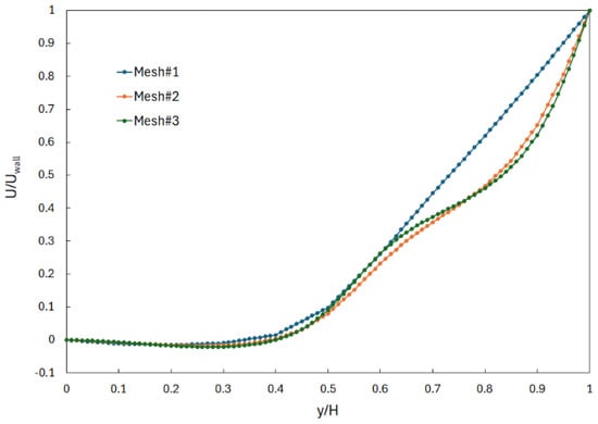
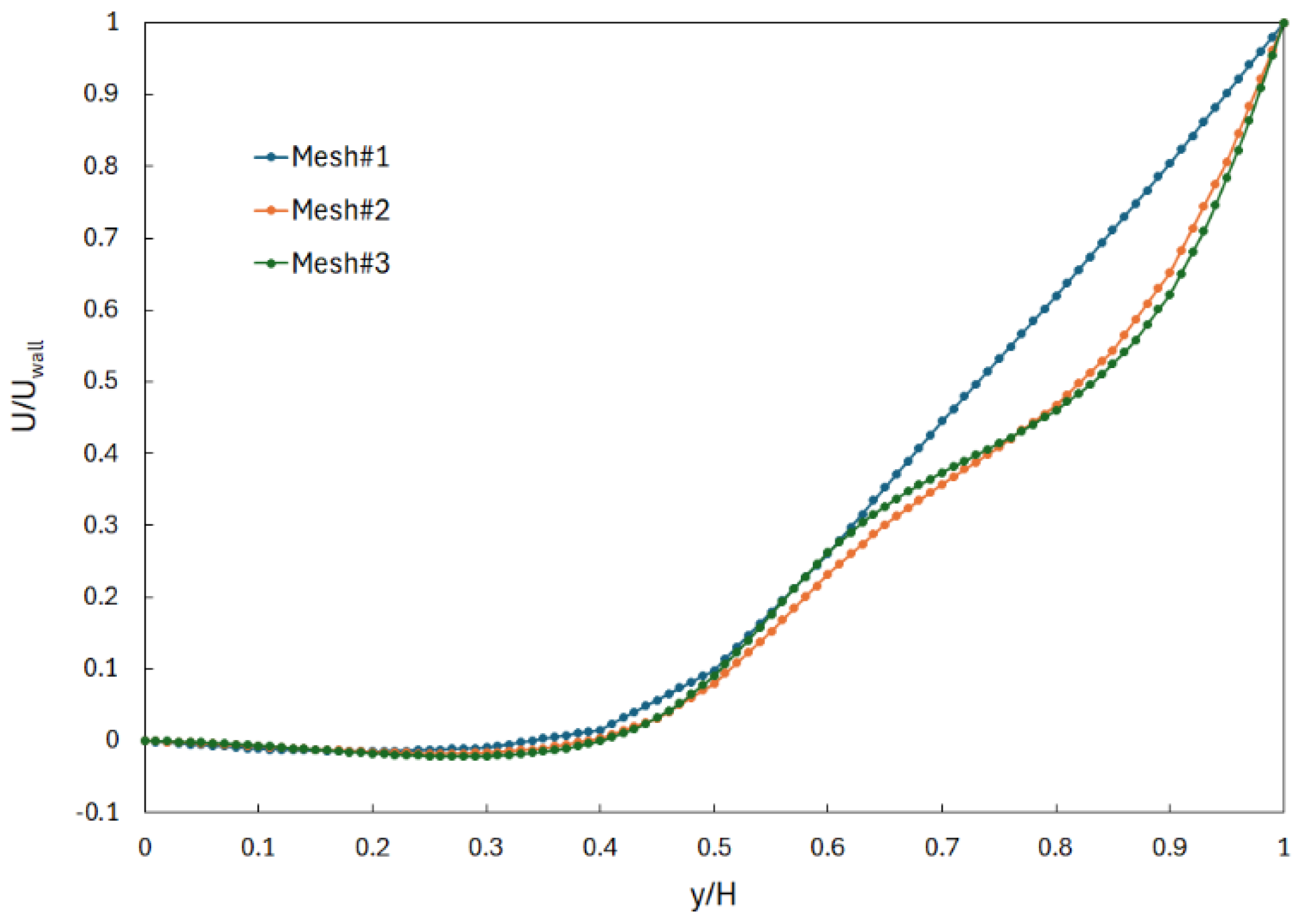
Figure 2 represents the grid independency results, which are obtained through the comparison of the mean velocity profile along the channel’s height at 0.5 mm downstream of the obstacle for the case h⁄H = 0.5. The simulations are carried out for three different cell numbers, Mesh#1, Mesh#2 and Mesh#3, as shown in Table 1. The numbers in Table 1 correspond to the mesh size in the rectangular cube with the dimension of L × L × H before the obstacle is subtracted from the geometry. As can be observed, the velocity distribution does not change significantly with an increase in the cell numbers from Mesh#2 to Mesh#3, suggesting the adequacy of Mesh#2 cell numbers in the present simulations. The small difference between the velocity profiles of Mesh#2 and Mesh#3 can be attributed to the presence of fibers in the simulations. Each simulation features unique positions of fibers within the flow, leading to slight variations in the results from Mesh#2 to Mesh#3. To further quantify the mesh sensitivity, the surface-time averaged shear stress on the upper wall was evaluated for Mesh #2 and Mesh #3. The corresponding values were 0.006525 and 0.006550 m2/s2, respectively, representing a relative difference of approximately 0.38%. This small variation, together with the close agreement of the downstream velocity profiles, indicates that further mesh refinement has a negligible effect on the predicted flow field and wall shear stress. Therefore, Mesh #2 was selected for the subsequent simulations as a suitable compromise between numerical resolution and computational cost. It should be noted that the maximum numbers of grids or the minimum size of meshes is limited by the particle size as the unresolved approach is used to perform simulations in the present study. It is recommended that the cell size be 3–10 times the size of the particles in this approach.
Figure 2.
The grid independency study for x-velocity 0.5 mm downstream of the obstacle.
Table 1.
Number of grid points used in the grid independency study.
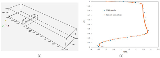
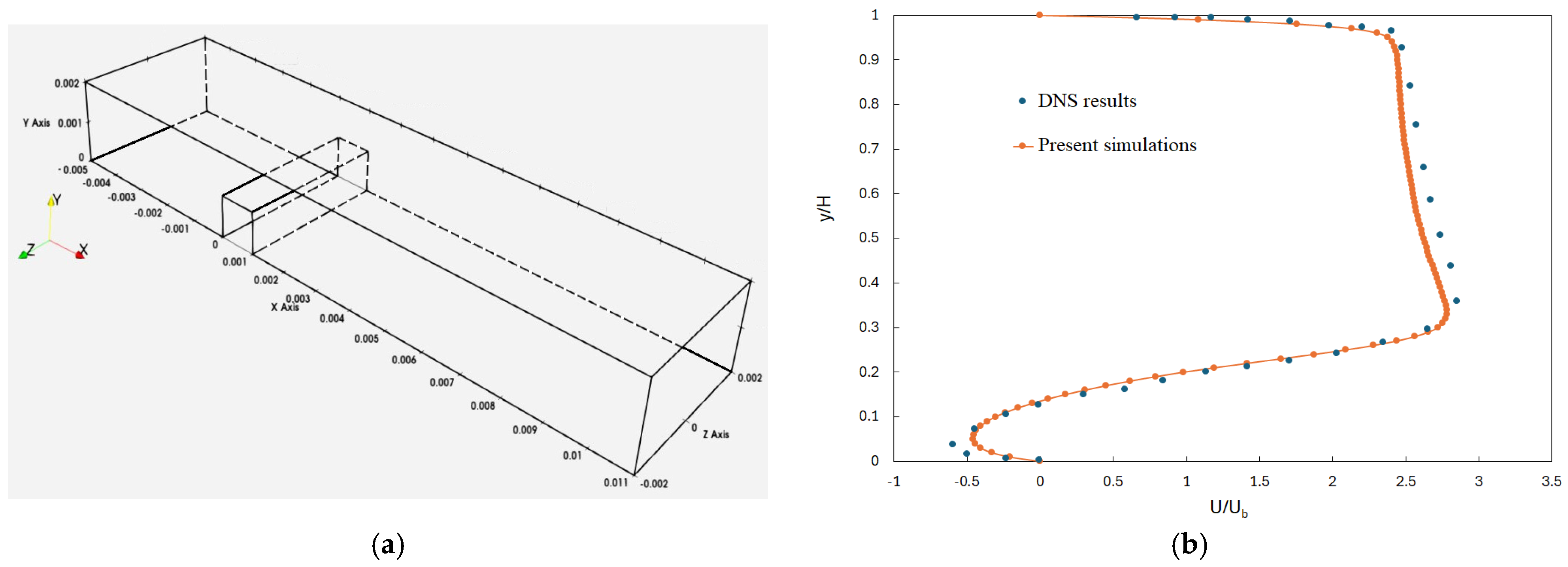
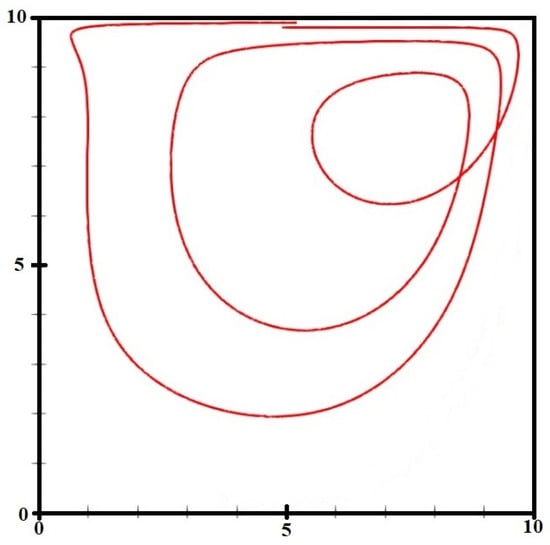
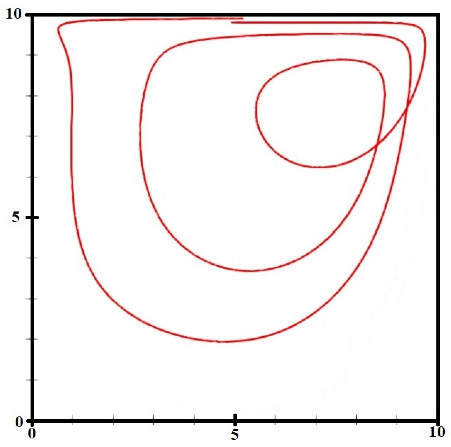
The CFD part of the simulation is validated by comparing the results with those reported by Kessler and Yang [20], obtained by DNS modeling of turbulent periodic flow in the channel with an obstacle shown in Figure 3a. The velocity distribution along the channel’s height at the middle of block is compared with the results reported by Kessler and Yang [20] in Figure 3b, where a good agreement is observed between the two sets of the results despite using the large eddy simulation (LES) method in the present simulations. In order to validate the CFD-DEM part of the simulations, the numerical simulation is carried out for a single particle in a three-dimensional cavity in Figure 4. The dimensions and operating conditions in the numerical simulation are selected to be similar to those reported in Tsorng et al.’s [21] experiments, i.e., a square cavity of side 10 cm in which a fluid with a viscosity of 37.2 mm2/s flows. A conveyer belt acts as a moving lid in the experiments with a velocity of 17.5 cm/s, which corresponds to Reynolds number 470. The particle is placed in a position in the middle and close to the lid. A good agreement is observed between the particle trajectory from the present numerical simulation and that of experimental measurements. However, the final orbit of the particle is not presented in Figure 4. According to Tsorng et al. [21], the final orbit of the particle is affected by the transient phase of the flow at the end of the measurements, a phenomenon that is not present in numerical simulations. The comparison with the experimental particle trajectories is qualitative, as the available experimental results do not provide sufficiently detailed numerical trajectory data for a reliable quantitative error assessment. Nevertheless, the numerical results reproduce the main features of the observed particle motion, supporting the suitability of the coupled CFD–DEM approach for the present investigation.
Figure 3.
(a) The geometry of the channel with obstacle used in Kessler and Yang [20]. (b) Comparison of x-velocity along the channel height with the DNS results from Kessler and Yang [20].
Figure 4.
Trajectory of a single particle in a cavity.
4.1. Flow Field
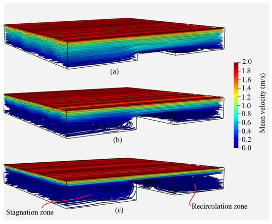
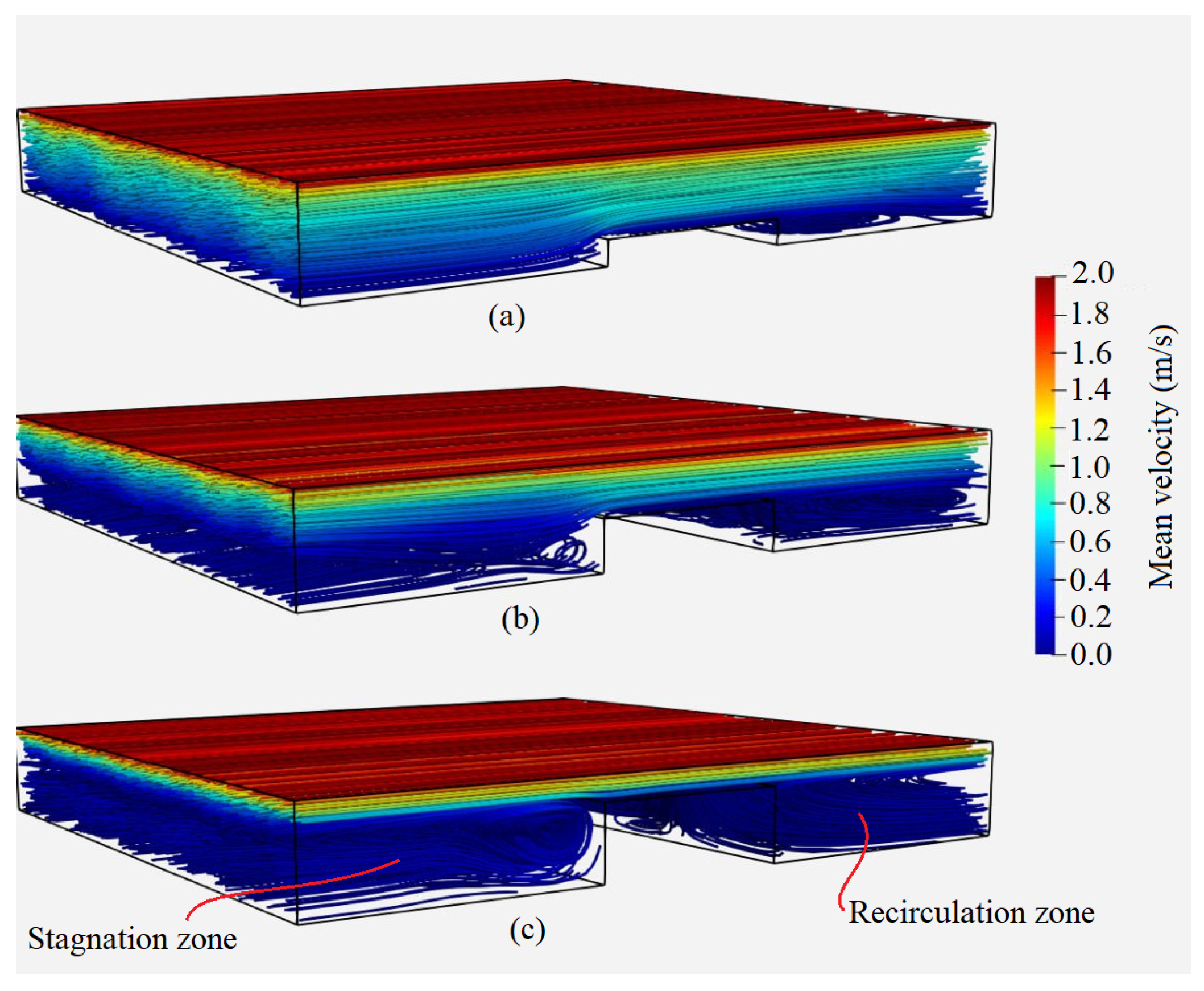
The change in the flow field, with a variation in the obstacle height, is shown in Figure 5 by illustrating the streamlines in different cases. The streamlines are colored with the mean velocity magnitude since the flow is found to be unsteady in the present simulations mainly due to the presence of fibers. As can be seen, the length of the recirculation zone downstream of the obstacle increases as the obstacle height increases. This can result in entrapment of larger numbers of fibers in the recirculation zone located far from the refining zone. The refining zone is defined as the region between the obstacle’s upper surface and the upper moving wall of the channel (see Figure 1). It can also be seen that in the case of h/H = 0.25 and h/H = 0.5, the momentum of the upper plate penetrates deeper into the fluid, causing a more effective mixing of entrapped fibers with fibers moving with the main flow. Meanwhile, a more channelized flow can be observed in the case of h/H = 0.75. It can also be seen that a stagnation zone is formed where the flow hits the obstacle and reverses direction as the obstacle height increases beyond h/H = 0.5. The interaction between the flow and fibers moving with the upper plate, as well as those entrapped within the stagnation and recirculation zones, plays an important role in the forces acting on fibers. The stagnation and recirculation zones are illustrated in Figure 5c.
Figure 5.
Streamlines in the channel for different obstacle heights: (a) (b) (c) .
4.2. Shear Stress Distribution
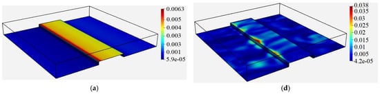
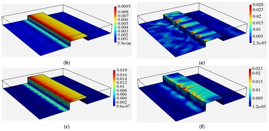
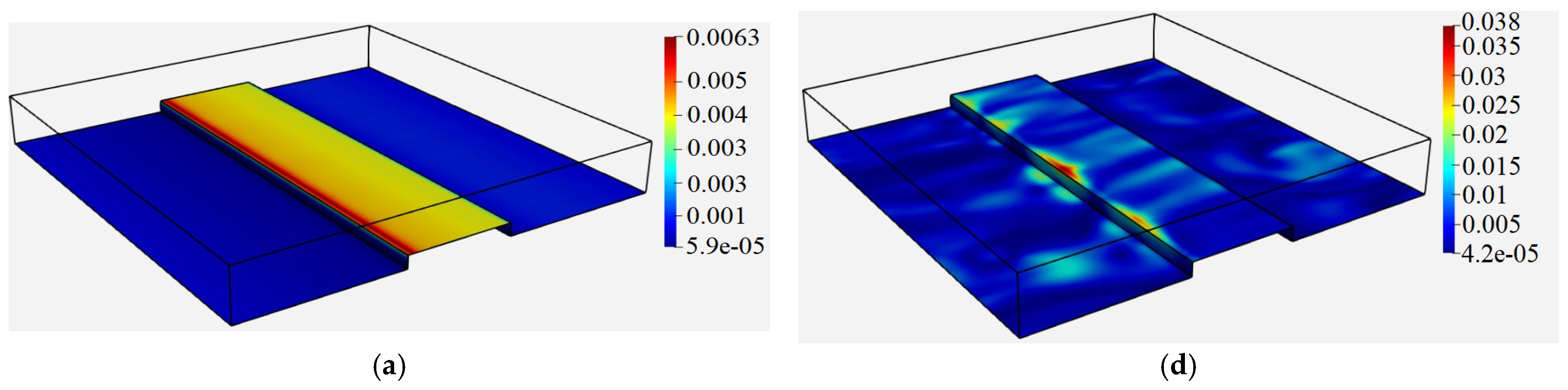
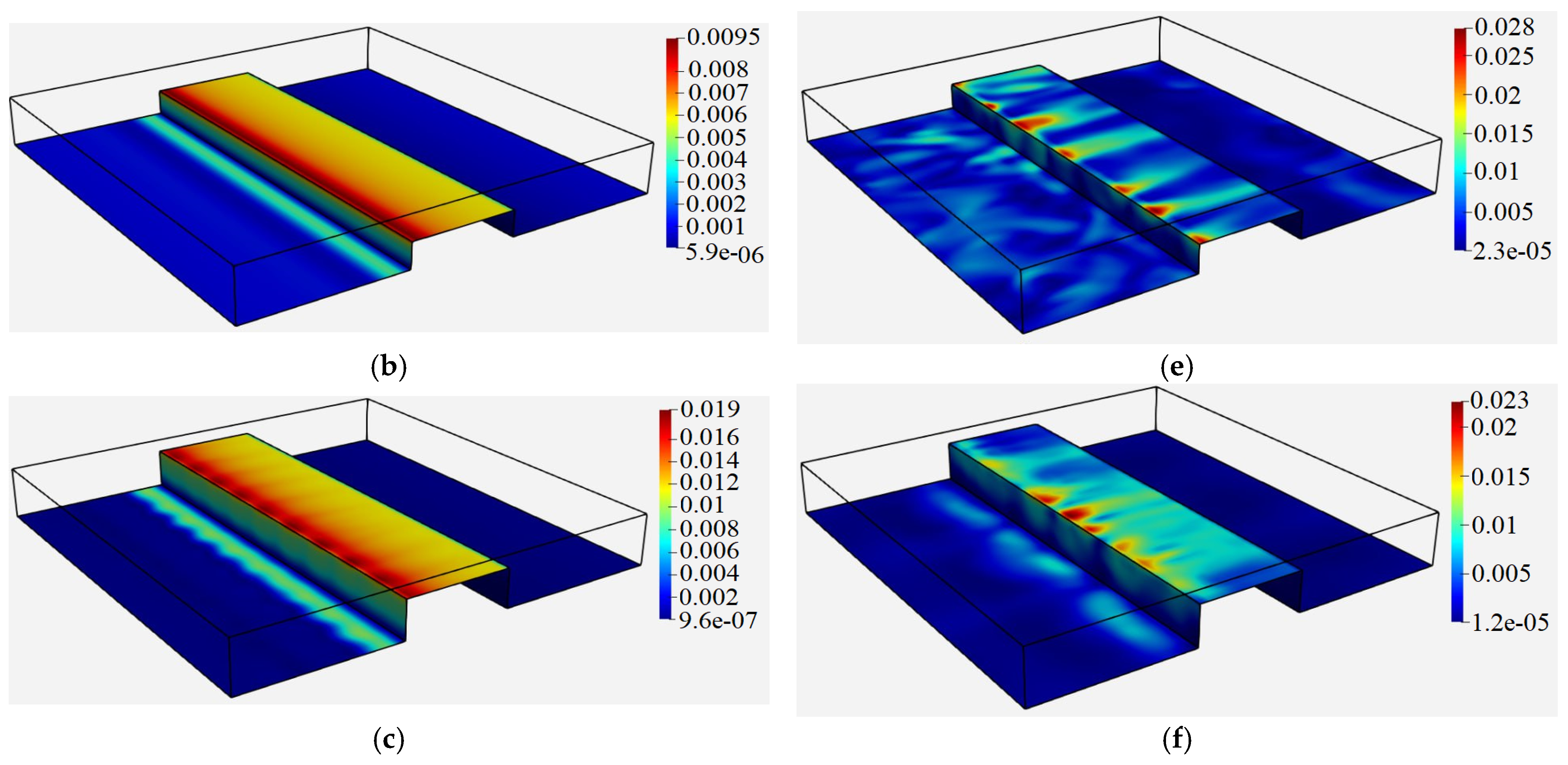
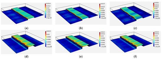
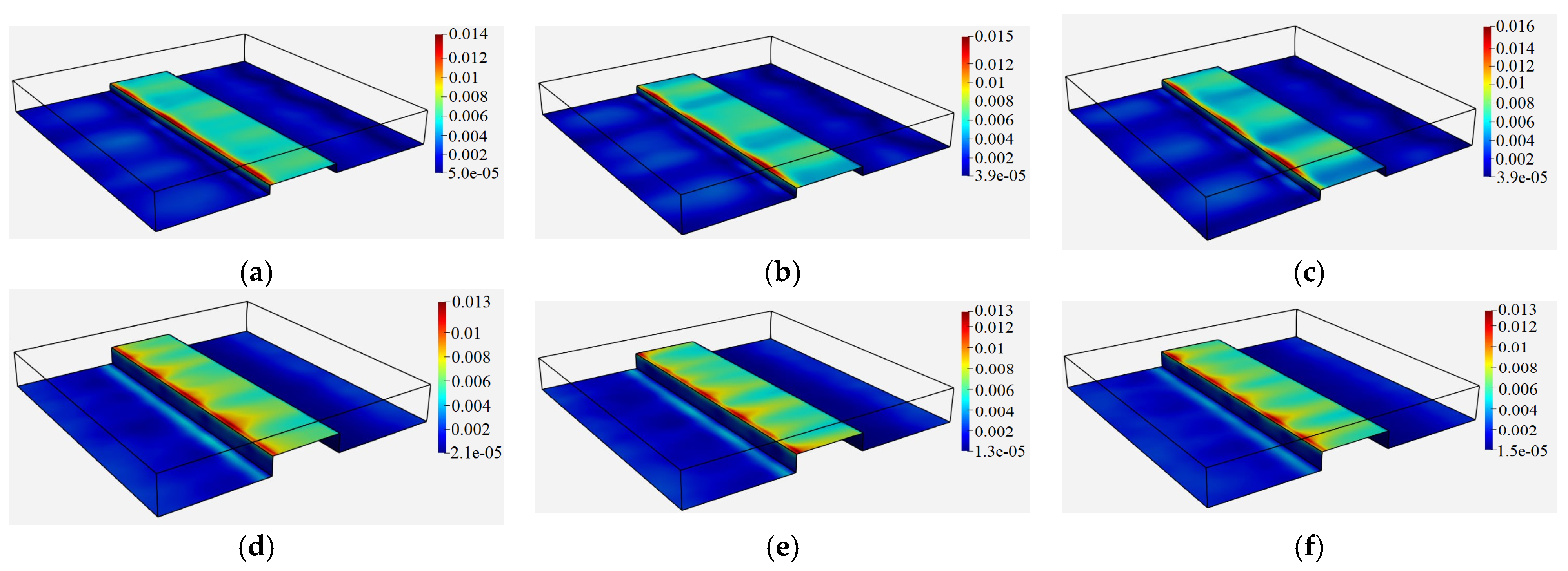
Figure 6 illustrates the shear stress distribution over the lower wall and the obstacle’s surface for different obstacle heights in the cases with and without fibers at the nondimensional time of . Here, the reported shear stress values are expressed in density-normalized form, /, and therefore have units of m2/s2. The same convention is used in Table 2 and the relevant figure captions. As can be seen, for cases without fibers, a larger obstacle leads to a larger shear stress at the obstacle surface. This is in agreement with the shear stress distribution in the refining region obtained using Couette flow hypothesis in a thin two-dimensional channel, where the shear stress is inversely proportional to the thickness of the channel:
where τ is the shear stress in the refining region, is the upper wall velocity and δ is the thickness of the refining region. However, the local distribution of shear stress in cases where fibers are present does not follow this trend. This can be attributed to the effect of fibers and their interaction with the walls and each other on the shear stress distribution. Another interesting effect of particles can be seen on the shear stress distributions on the lower wall ahead of the obstacle. Unlike the cases without fibers where an increase in the shear stress over the lower wall can be seen over a strip for h/H = 0.50 and h/H = 0.75 upstream of the obstacle, the pockets of higher shear stress can be seen to be spread upstream and downstream of the obstacle in the cases where fibers are present. The higher shear stress region in the form of a strip comes back in the case of h/H = 0.75 with fibers showing that the effect of fluid flow on the shear stress upstream of the obstacle becomes increasingly important when the obstacle’s height is increased and a stronger downflow is formed at the obstacle’s upstream side. The more uniform shear stress distribution on the obstacle’s upper surface in Figure 6f, compared with Figure 6d,e, indicates a more spatially uniform distribution of the computed surface shear stress under this condition. The smaller refining-region thickness may contribute to the observed interaction between the fibers and the obstacle surface. Although the present simulations do not directly quantify fibrillation, the results may be relevant to understanding how obstacle geometry influences the distribution of mechanical loading in refining applications. The results presented here for the shear stress distribution over the obstacle’s top surface in Figure 6d–f agree with the observations made by Martinez et al. [5] regarding the sharp increase in force over the first 2–3 mm of the bar.
Figure 6.
Shear stress distribution in without fibers: (a) (b) (c) and in the presence of fibers (d) (e) (f)
Table 2.
The surface-time averaged values of shear stress over the obstacle’s upper surface in .
Further investigation of the shear stress on the upper surface of the obstacle was performed by comparing the surface-time averaged values for the three cases reported in Table 2. The results show that, for h/H = 0.25, the presence of fibers increases the averaged shear stress. For h/H = 0.5, the averaged shear stress remains nearly unchanged, increasing only slightly from 0.0064 to 0.00658 . In contrast, for h/H = 0.75, the presence of fibers decreases the average shear stress. The increase observed for h/H = 0.25 may be associated with the wider refining region, which allows greater fiber motion and interaction with the obstacle surface. These interactions may contribute to the observed increase in local shear stress. For h/H = 0.75, the narrower refining region is associated with fiber stapling and the formation of a fiber layer near the obstacle’s upstream edge and upper surface. This configuration may reduce the exposure of parts of the obstacle surface to the surrounding flow and may contribute to the lower surface-time averaged shear stress. For (h/H = 0.5), the relatively small change in the averaged shear stress suggests that the effects of fiber motion and fiber–obstacle interaction on the surface stress are limited under the conditions considered.
4.3. Forces Acting on Fibers
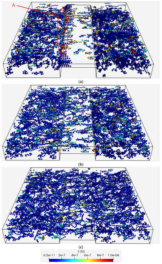
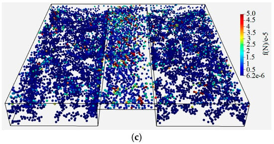
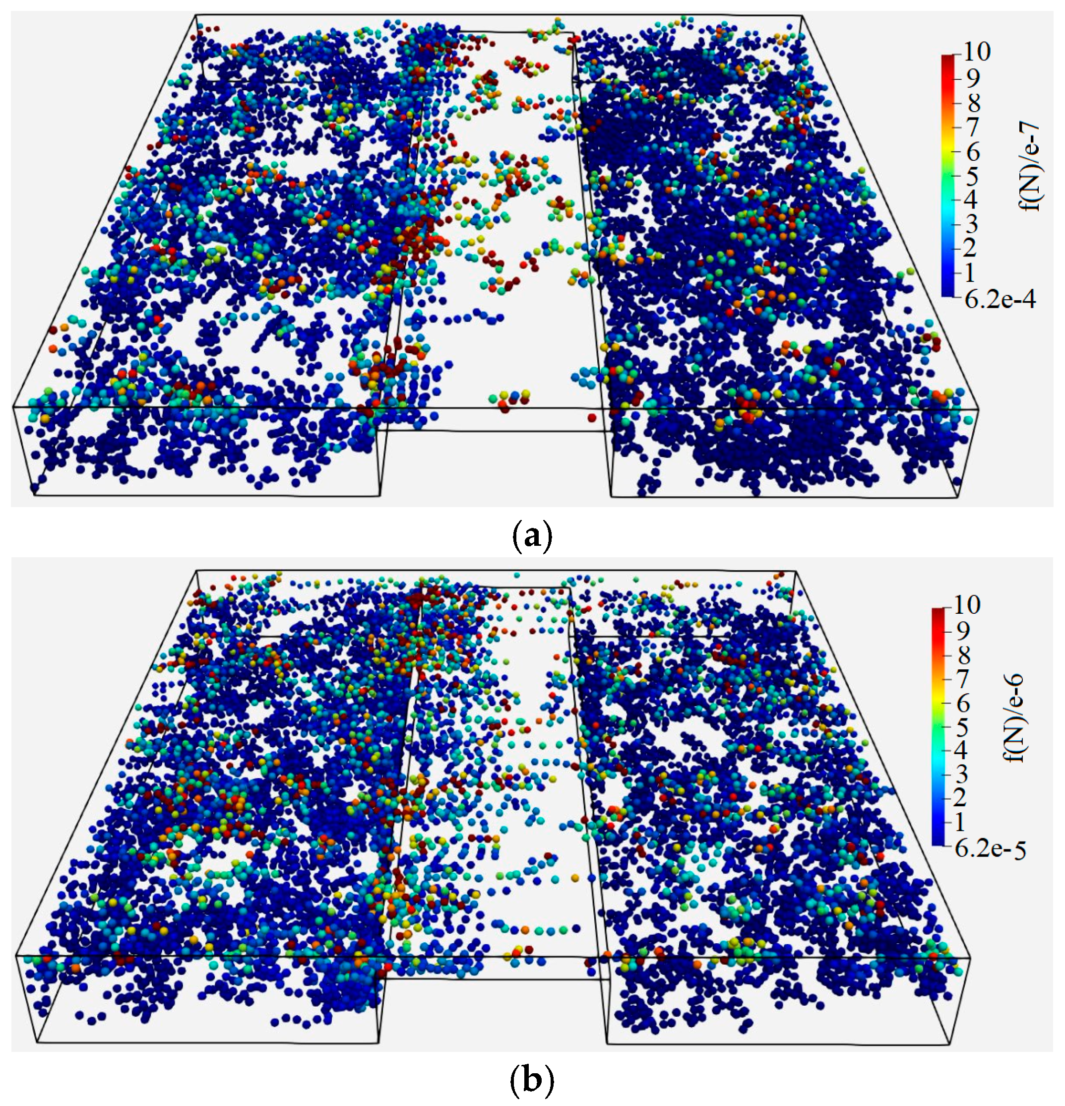
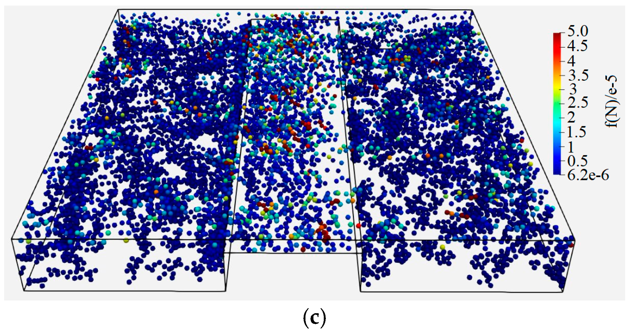
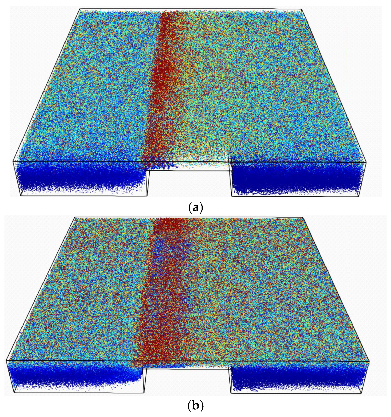
Forces acting on fibers at higher consistency are illustrated in Figure 7a–c, where approximately 1300 fibers are present in the solution domain for all three obstacle heights. For h/H = 0.75 (Figure 7a), fibers tend to become stapled at the upstream edge of the obstacle. In this region, incoming fibers may experience forces associated with contact interactions with previously stapled fibers, as well as hydrodynamic forces arising from the surrounding flow and interactions with neighboring moving fibers, as indicated in region A of Figure 7a. The motion of the upper wall also contributes to the force levels in the refining region. For h/H = 0.75, the velocity gradients associated with the stagnation and recirculation regions may further influence the forces acting on the fibers. For h/H = 0.5 (Figure 7b), the stapling mechanism is not observed, and the shear forces induced by the upper wall appear to be more evenly distributed among the adjacent fibers. For h/H = 0.25 (Figure 7c), the fibers are less affected by the shear from the moving upper wall than in the h/H = 0.5 and h/H = 0.75 cases. This may be attributed to the weaker or absent backflow and recirculation zones upstream and downstream of the obstacle at the lowest obstacle height.
Figure 7.
Forces acting on fibers for almost 1300 fibers in (a) (b) (c) .
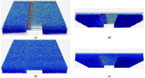
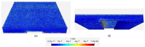
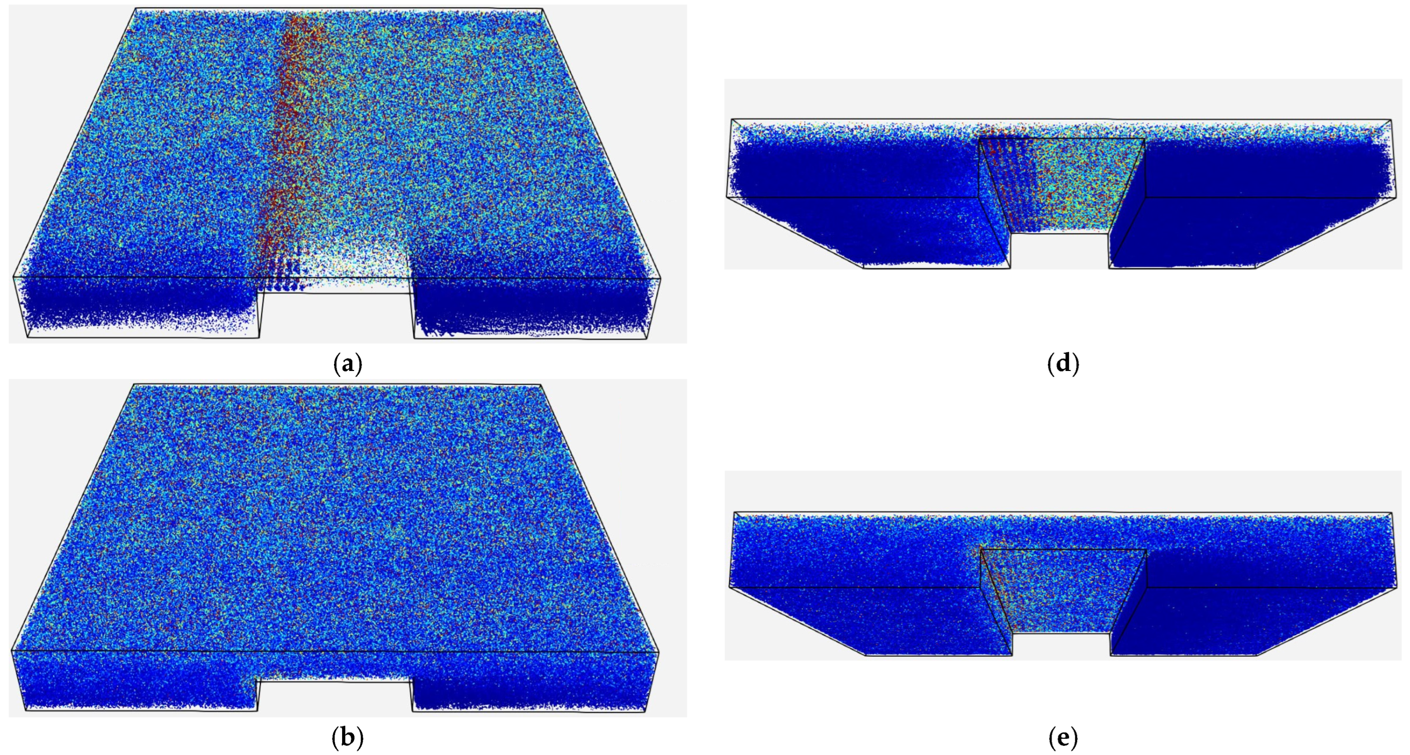
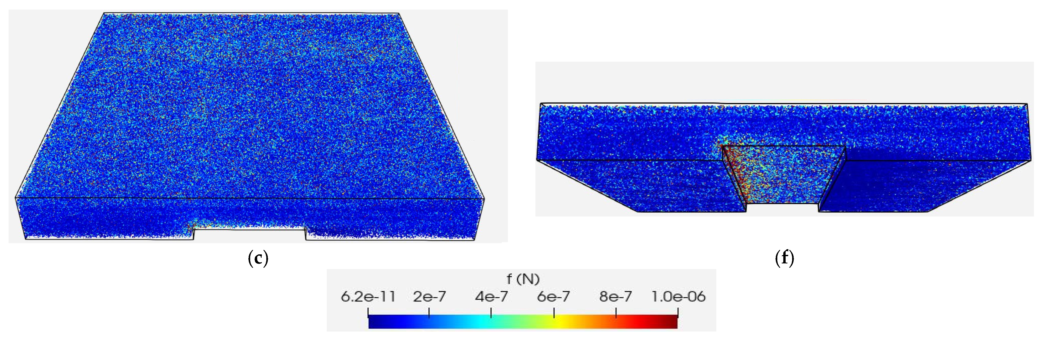
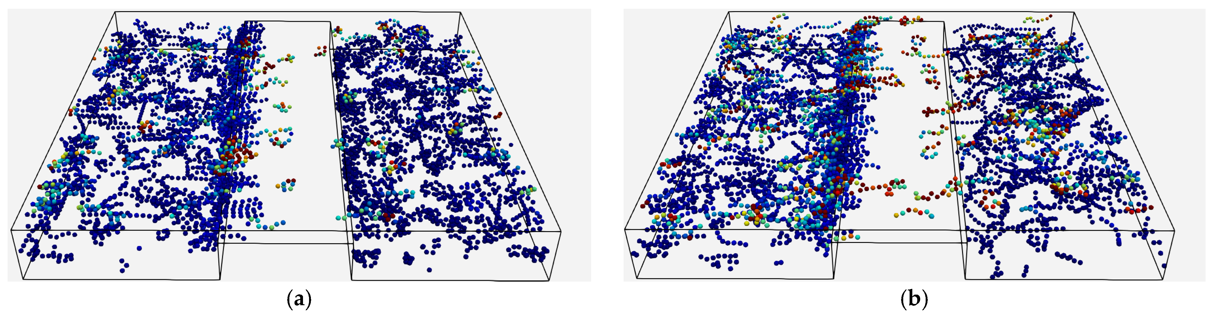
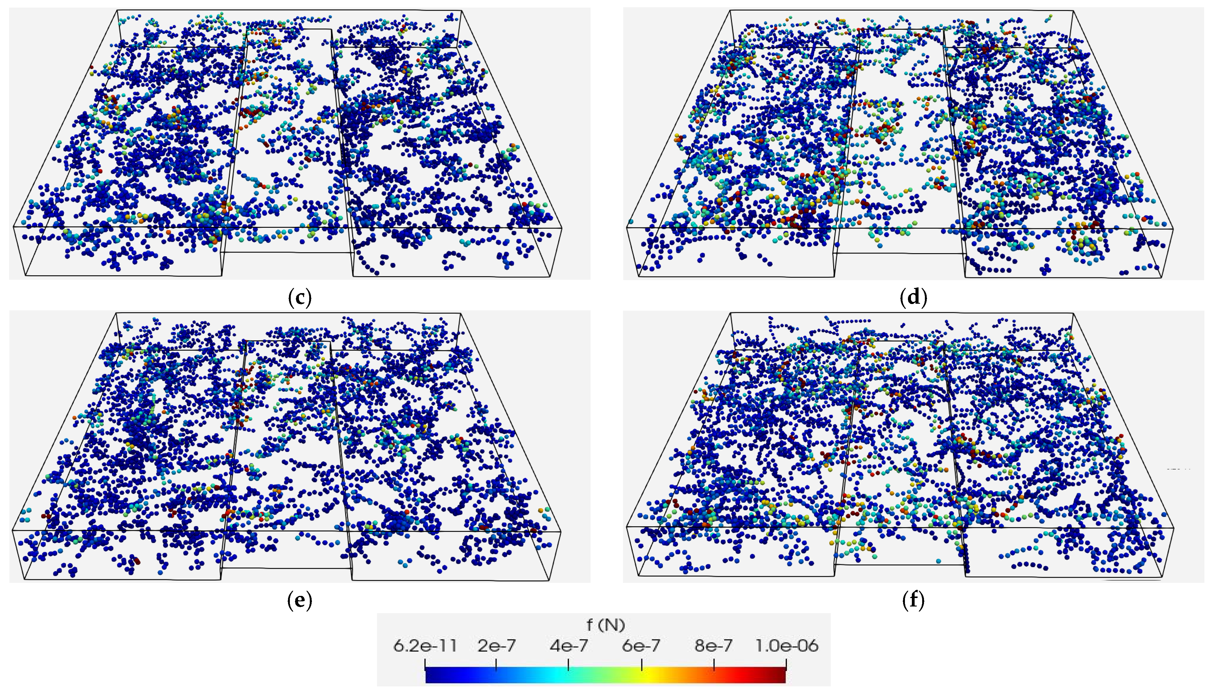
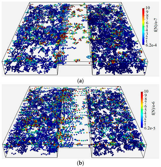
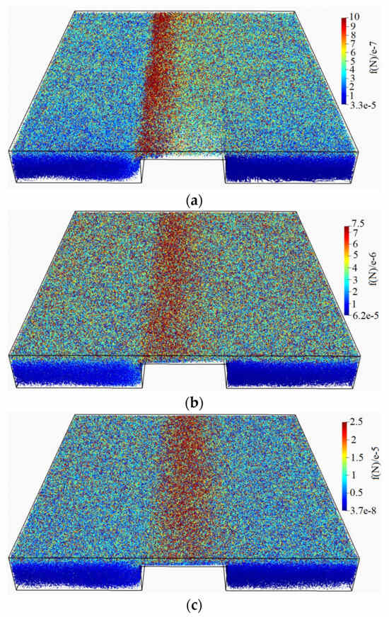
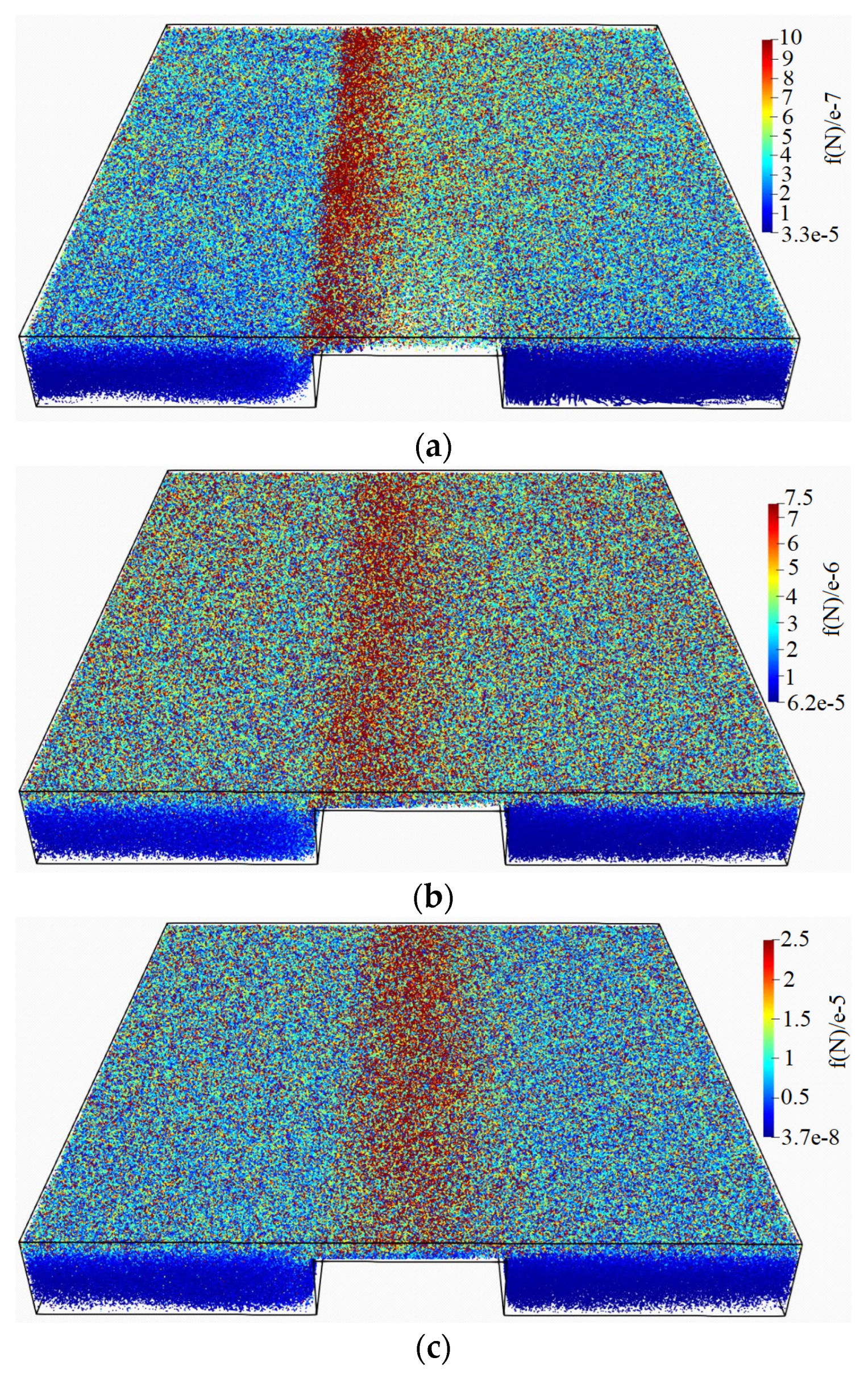
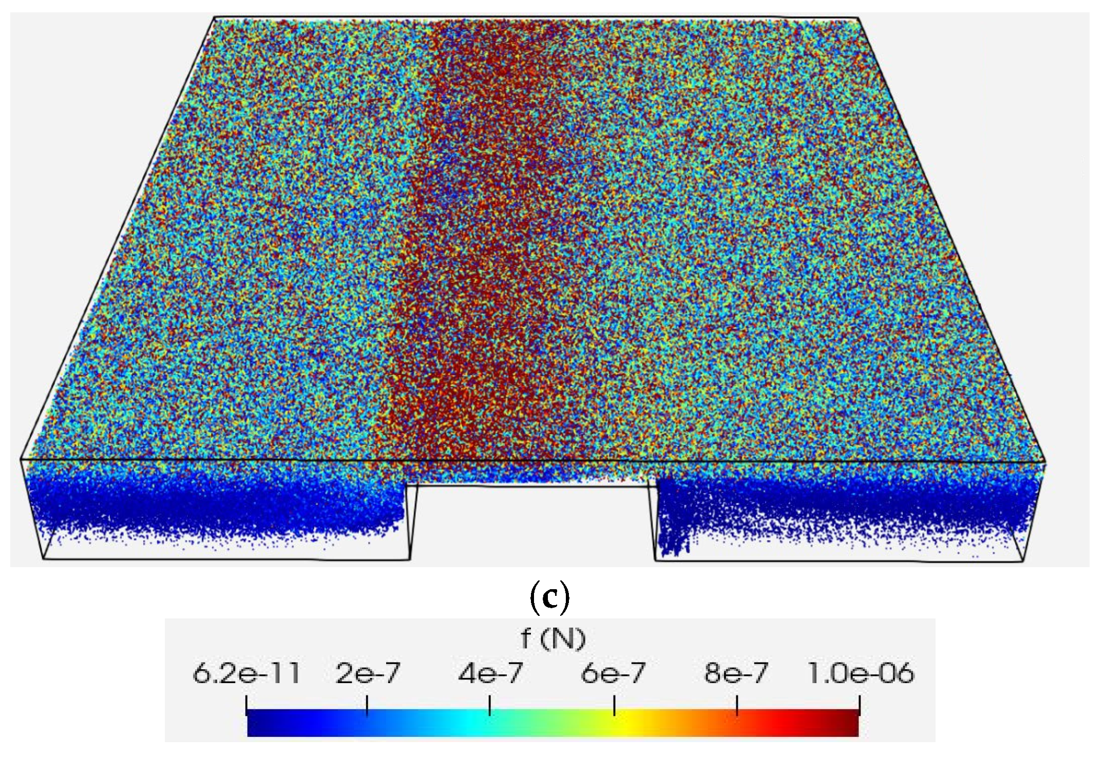
To further examine the force distribution, the forces acting on fibers at all time steps are compiled together in Figure 8. Two views are provided to illustrate these forces: a top view and a view from underneath the channel. It is evident that the corner forces are more pronounced due to fibers becoming stapled at the obstacle’s upstream edge in the cases of h/H = 0.75 (see Figure 8a) and h/H = 0.25 (see Figure 8f) compared to h/H = 0.50. It is noteworthy that the flow patterns in the refining region differ significantly between h/H = 0.75 and the other cases studied here. In the former, a stagnation point with high stagnation pressure forms at the obstacle’s upstream edge and the flow in the refining region resembles closely the Couette flow in a thin slit. The stagnation of flow at the obstacle’s upstream edge results in an effective stapling of fibers in this case. This effect, combined with the impact and shear from incoming particles and the upper wall, creates a region with higher force levels at the entrance of the refining region in h/H = 0.75. As the obstacle height decreases and the refining region widens in h/H = 0.25 and h/H = 0.50, the flow deviates from the Couette flow principle. A velocity boundary layer begins to form over the upper surface of the obstacle in these cases. Flow comes to rest at the tip of the velocity boundary layer, providing a favorable condition for fibers to become stapled at the upstream edge of the obstacle. However, the upper wall’s momentum affects a significant portion of the flow at the entrance of the refining region in h/H = 0.50, hindering the stapling of fibers at the obstacle’s edge. With a larger proximity to the upper moving wall in h/H = 0.25, the fibers can get stapled at the obstacle’s upstream edge where the boundary layer tip is located. This stapling in combination with impact from incoming particles creates a region with a higher force level at this location (see Figure 8f).
Figure 8.
Forces acting on fibers at all timesteps: (a,d) , (b,e) , (c,f) .
4.4. Flexibility
In order to study the effect of fiber’s flexibility, a dimensionless number is defined here as
where L is the fiber length, is the shear rate in the channel, μ is the fluid’s viscosity, is a coefficient related to the bond’s shear properties and length and is the second moment of inertia. A high means that fluid forces acting on fibers dominate, leading to significant fiber bending and deformation. A low indicates that the fiber remains relatively stiff in the flow. In the cases presented here, the fluid viscosity, the upper wall velocity and fiber geometry are kept constant, while the effect of fiber stiffness on the shear stress and force distribution is investigated by varying the . Three different values of are examined: 10, 1 and 0.1. The flexibility parameter is varied by changing the tangential bond stiffness, , in Equation (11). The values , , and correspond to , 1, and 0.1, respectively. A comparison of the results for the case where 660 particles are present in the solution domain is carried out in Figure 9. It can be observed that the number of fibers affected by the shear generated by the movement of the upper wall increases with a decrease in in the cases h/H = 0.50 and h/H = 0.25. This trend may be related to the reduced ability of stiffer fibers to bend and conform to the flow. Their more limited deformation may result in different force distributions and greater localized force magnitudes compared with more flexible fibers, which can accommodate the flow more readily. This observation agrees with the previous observations in the pulp refining process where the chemical pulp’s ability to get refined in the refiner is not as much as that of mechanical pulps due to, among other things, their softness after being chemically treated.
Figure 9.
Forces acting on fibers for different obstacle heights and fiber stiffness: (a,b) , (c,d) , (e,f) . Left column shows fibers with a and the right column .
The effect of fiber stiffness on the time-averaged shear stress is shown in Figure 10. For h/H = 0.75, the average shear stress decreases as fiber stiffness increases. This trend may be associated with the fiber configurations observed near the entrance of the refining region, where the accumulation of relatively stiff fibers may influence the local flow and fiber motion within the narrow gap. The reduced ability of stiffer fibers to conform to the flow may also affect their interaction with the obstacle surface. However, the relative contributions of fiber accumulation, orientation, and fluid-mediated momentum transfer are not separately quantified here. In contrast, for h/H = 0.25, an opposite trend is observed. In this wider refining region, the greater available space for fiber motion and interaction with the obstacle edge may allow stiffness-dependent differences in fiber–obstacle interaction to influence the computed shear stress more strongly. The case h/H = 0.5 lies between these two conditions, where the competing effects of fiber configuration and fiber–obstacle interaction may contribute to the relatively small changes in averaged shear stress with fiber stiffness.
Figure 10.
The time averaged values of shear stress in over the top surface of the obstacle for different obstacle heights and fiber stiffness: (a–c) , (d–f) , (g–i) . Left column shows fibers with , the middle column and right column .
4.5. Upper Wall Velocity
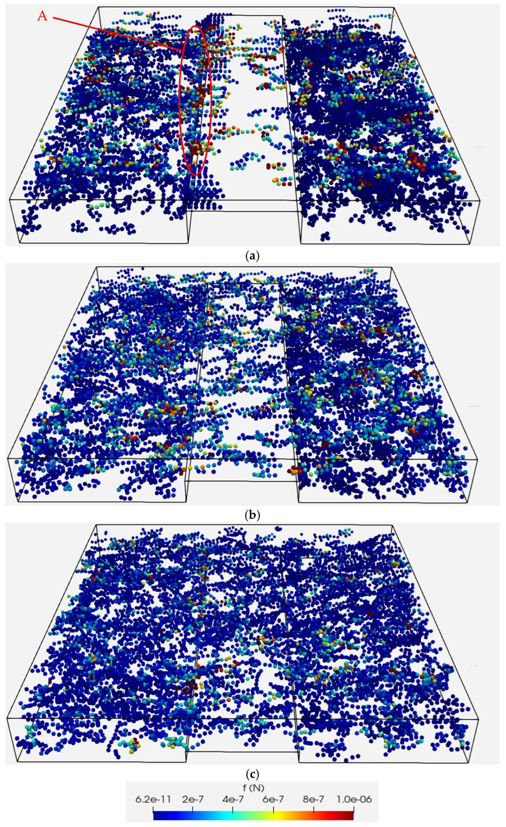
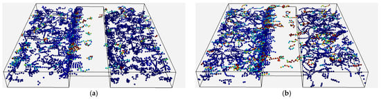
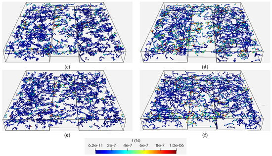
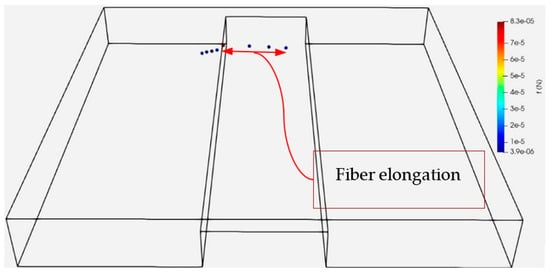
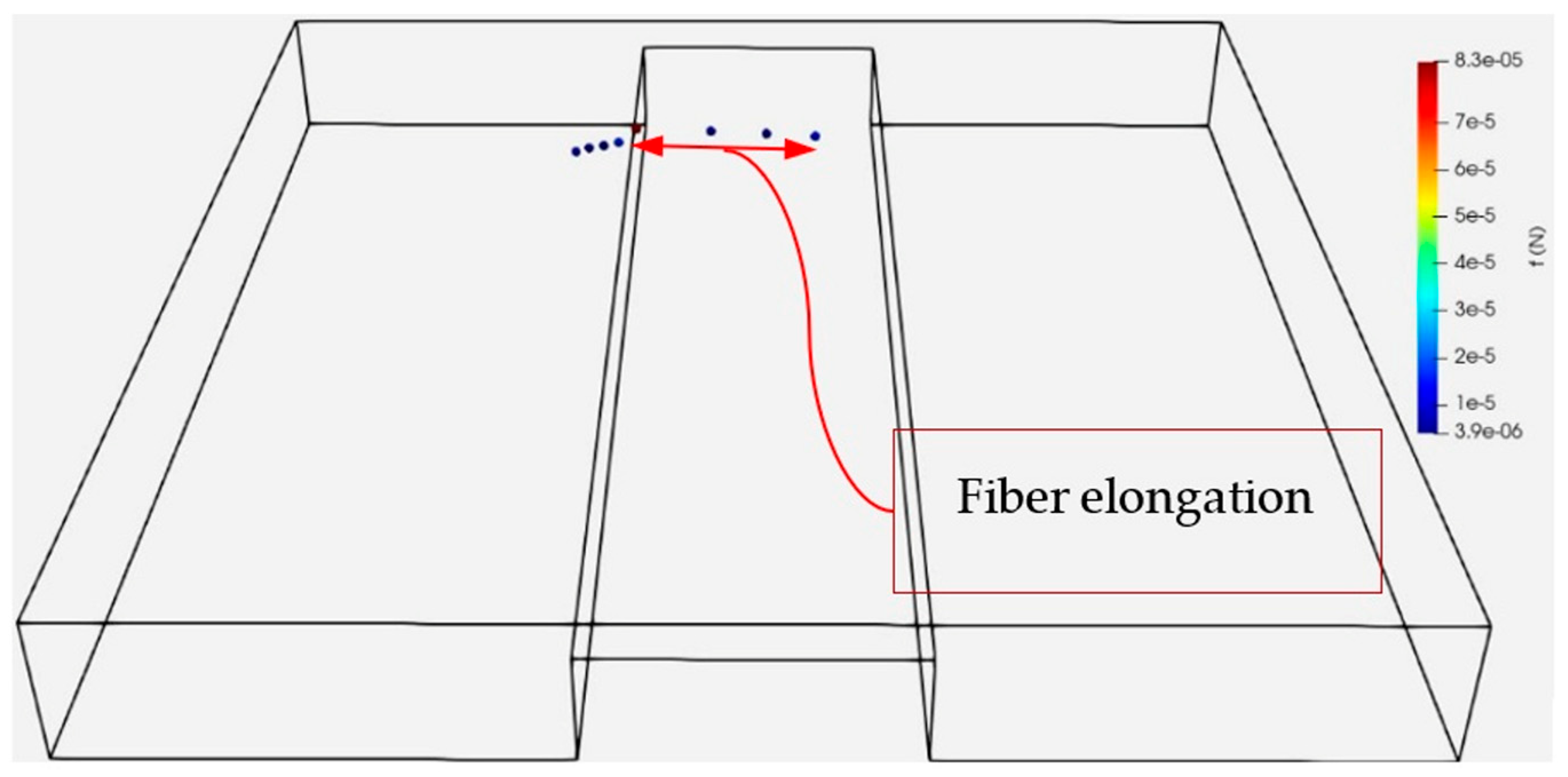
The effect of upper wall’s velocity on the stapling of fibers and forces acting on fibers is investigated in Figure 11 for the cases where almost 1300 fibers are present in the solution domain. The simulations are carried out for the h/H = 0.75 and for three different velocities = 2 m/s, = 10 m/s and = 20 m/s. As shown in Figure 11, the tendency for fibers to become stapled at the upstream edge of the obstacle decreases as the upper wall velocity increases, accompanied by a change in the force distribution at = 20 m/s. At the higher velocities, the force patterns appear to be more strongly associated with the flow in the refining region, whereas the lower-velocity case also shows force concentrations in regions where moving fibers interact with previously stapled fibers. These observations suggest that the relative influence of hydrodynamic and contact interactions changes with upper wall velocity, although their individual contributions are not separately quantified. These interactions are at least one order of magnitude greater in the case of = 20 m/s compared to those in the base case simulations, = 2 m/s. This effect would be even more pronounced in the operating condition in a real refiner where the edges of the bars (obstacles) are not as sharp as those in the simulations causing even fewer fibers to get stapled in the real conditions. To provide a complete overview, forces acting on fibers at different speeds of the upper moving wall across all time steps are compiled in Figure 12. As the speed of the upper wall increases, it can be observed that the region of maximum forces on the fibers shifts downstream along the obstacle’s surface, which agrees with the earlier results in Figure 11. Additionally, due to larger shear forces exerted by the upper moving wall, the maximum forces acting on fibers at = 20 m/s are an order of magnitude larger than those at = 2 m/s. Another important phenomenon that is observed at higher velocities is the stretching of fibers (see Figure 13) at the edge of the obstacle, which can lead to tensile failure in a real refiner. This mechanism is believed to be more effective in the shortening of fibers than the scissor-like shearing according to Heymer [22]. However, such a fiber shortening cannot be captured in the present simulations since the fibers are modeled as an elastic chain of spheres without a model for fiber cutting.
Figure 11.
Forces acting on fibers in for different velocities of the upper wall: (a) , (b) , (c)
Figure 12.
Forces acting on fibers at all time steps in for different velocities of the upper wall: (a) , (b) , (c)
Figure 13.
Tensile forces on fibers trapped at the obstacle edge in and .
4.6. Fiber Length
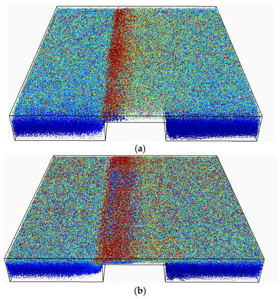
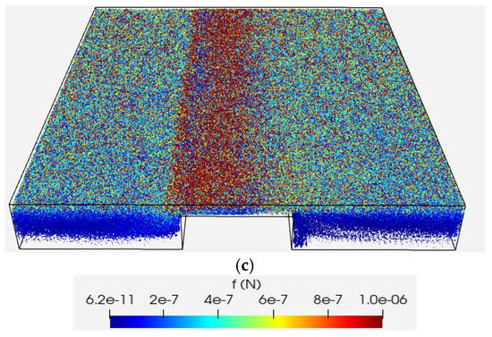
The effect of fiber length on the forces acting on fibers is investigated in Figure 14 by varying the fiber aspect ratio from the original 8:1 used in previous simulations to 12:1 and 16:1. As the fiber length increases, enhanced fiber–fiber and fiber–wall interactions are observed, particularly in the refining region. This is evident from the widening of the red-colored area in the refining region for the 16:1 aspect ratio, indicating stronger forces or more frequent interactions in this region compared to shorter fibers. These results suggest that longer fibers experience more pronounced interaction dynamics, which could significantly influence their behavior within the flow, particularly when encountering obstacles. However, the blue patches observed at the beginning of the refining region in Figure 14b,c indicate that the impacts in these cases are not as effective as those shown in Figure 14a. This can be attributed to the tendency of longer fibers to cover the obstacle’s upstream edge more thoroughly than shorter fibers, leading to softer impacts when incoming fibers interact with the obstacle edge.
Figure 14.
Forces acting on fibers at all time steps in h⁄H = 0.75 for different aspect ratios of fiber: (a) 8:1, (b) 12:1, (c) 16:1.
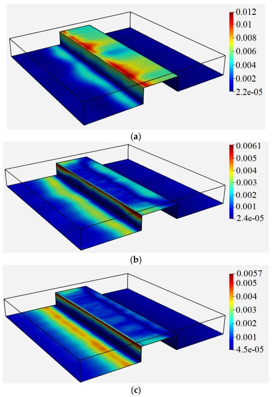
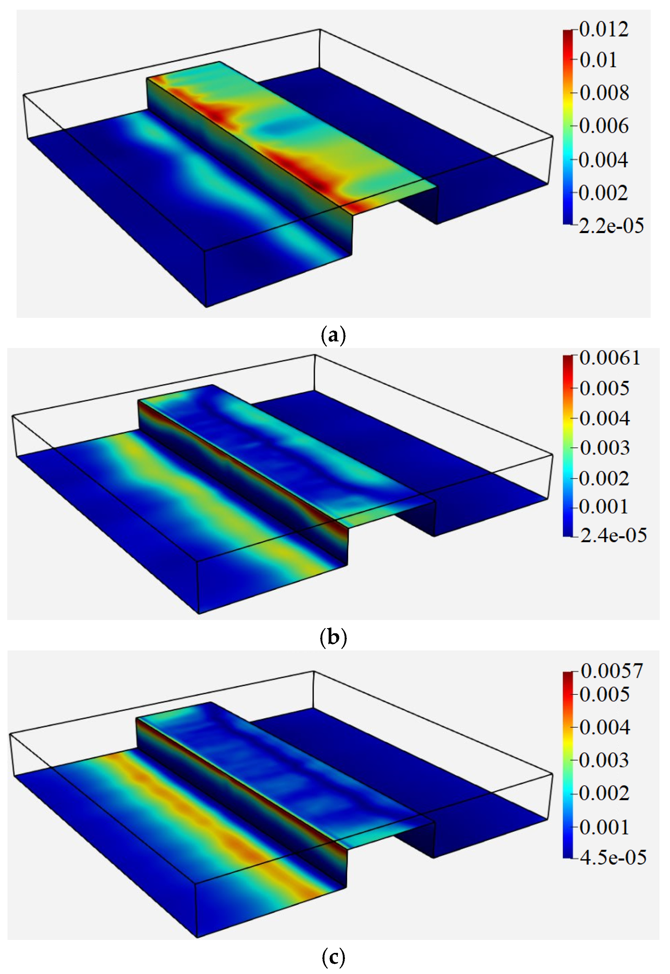
Figure 15 illustrates the time averaged shear stress distribution over the obstacle walls for three different lengths of fibers discussed above. As can be seen, the time-averaged shear stress over the obstacle’s top surface decreases with an increase in the fiber length. Longer fibers tend to align more with the flow direction because of their higher aspect ratio. This alignment modifies the local flow field around the obstacles and reduces the disturbance of the flow near the obstacle surface, resulting in a lower shear stress.
Figure 15.
Time averaged shear stress in m2⁄s2 over the channel and obstacle surfaces in h⁄H = 0.75 for different aspect ratios of fiber: (a) 8:1, (b) 12:1, (c) 16:1.
5. Conclusions
Numerical simulations were performed using a coupled CFD–DEM approach to investigate fiber–obstacle interaction, fiber entrapment, and shear stress distribution in a channel flow. The results show that obstacle height strongly modifies the flow structure and, consequently, the way fibers interact with the obstacle. Increasing the obstacle height enlarges the stagnation and recirculation regions and promotes fiber accumulation near the upstream edge of the obstacle.
The results show that the presence of fibers does not have a uniform effect on the shear stress acting on the obstacle. Compared with the fiber-free cases, the surface-time averaged shear stress increased by approximately 68% for h/H = 0.25, changed by only about 3% for h/H = 0.50, and decreased by approximately 31% for h/H = 0.75. The reduction at the highest obstacle was associated with fiber stapling and the formation of a fiber layer over the upstream edge and obstacle surface, which partially shields the surface from the main flow. This demonstrates that fiber accumulation can either enhance or reduce momentum transfer to the obstacle depending on the available refining gap.
The simulations also show that the forces acting on fibers result from the combined effects of upper wall shear, fiber–fiber interaction, and impacts with stapled fibers. Fiber flexibility changes this balance: stiffer fibers produce stronger localized interactions in the wider refining region, whereas in the narrow refining region they tend to accumulate near the obstacle entrance and reduce momentum transfer to the obstacle. Increasing the upper wall velocity reduces fiber stapling and changes the dominant force mechanism from impact toward shear, with the fiber forces increasing by approximately one order of magnitude between = 2 m/s and 20 m/s. Increasing fiber length enhances fiber–fiber and fiber–wall interactions while reducing the shear stress on the obstacle surface, mainly because longer fibers align more readily with the flow and cover the obstacle surface.
Overall, the results show that fiber–obstacle interaction is governed by the coupled effects of obstacle geometry, fiber arrangement, flexibility, length, and flow velocity. The CFD–DEM approach therefore provides a means of resolving these interactions and identifying the mechanisms controlling fiber forces and momentum transfer at an obstacle, which are relevant to understanding fiber treatment in refining flows.
Author Contributions
Conceptualization, N.F. and B.A.E.; methodology, N.F., J.P. and B.A.E.; software, N.F. and J.P.; investigation, N.F.; resources, B.A.E.; data curation, N.F.; writing—original draft preparation, N.F.; writing—review and editing, J.P. and B.A.E.; project administration, B.A.E.; funding acquisition, B.A.E. All authors have read and agreed to the published version of the manuscript.
Funding
The work was conducted within the research profile Neopulp (KKS-DNR 20210009) financed by the Knowledge Foundation and cofunded by the European Union.
Data Availability Statement
The original contributions presented in this study are included in the article. Further inquiries can be directed to the corresponding authors.
Conflicts of Interest
The authors declare no conflicts of interest.
Nomenclature
| Symbol | Definition | Unit |
| Fluid volume fraction | – | |
| Time | s | |
| Fluid velocity vector | m/s | |
| Resolved fluid velocity vector | m/s | |
| Particle/solid velocity vector | m/s | |
| i-th component of the resolved velocity vector | m/s | |
| j-th spatial coordinate | m | |
| Fluid density | kg/m3 | |
| Pressure | Pa | |
| Implicit fluid–solid momentum exchange coefficient | kg/(m3·s) | |
| Gravitational acceleration vector | m/s2 | |
| Resolved velocity gradient tensor | 1/s | |
| Resolved strain rate tensor | 1/s | |
| Deviatoric symmetric tensor form from | 1/s2 | |
| Explicit fluid–solid momentum exchange term | kg/(m2·s2) | |
| Drag force acting on a particle | N | |
| CFD cell volume | m3 | |
| Fluid kinematic viscosity | m2/s | |
| SGS kinematic eddy viscosity | m2/s | |
| Effective viscosity | m2/s | |
| Wale model constant | – | |
| Filter width or characteristic cell length | m | |
| Kronecker delta | – | |
| I | Identity tensor | – |
| Mass of particle | kg | |
| Velocity of particle | m/s | |
| Moment of inertia of particle | kg·m2 | |
| Angular velocity of particle | s−1 | |
| Contact force on particle | N | |
| Bond force on particle | N | |
| Fluid force on particle | N | |
| Body force on particle | N | |
| Contact torque on particle | N·m | |
| Bond torque on particle | N·m | |
| External torque on particle | N·m |
References
- Lumiainen, J. Refining of chemical pulp. In Papermaking. Part 1: Stock Preparation and Wet End; Paulapuro, H., Ed.; Fapet Oy: Helsinki, Finland, 2000; Chapter 4; Available online: https://turbulence-initiated.sites.olt.ubc.ca/files/2013/01/1998-Lumiainen-Ch4.pdf (accessed on 6 June 2026).
- Nugroho, D. Low Consistency Refining of Mixtures of Softwood and Hardwood Bleached Kraft: Effects of Refining Power. Master’s Thesis, Asian Institute of Technology, Pathum Thani, Thailand, 2012. Available online: https://www.fibrelab.ubc.ca/files/2012/07/LCRefining_Mixed-Softwood-Hardwood_Dimas-Thesis_.pdf (accessed on 23 June 2026).
- Introduction to Stock prep Refining. 2016. Available online: https://aft-global.com/sites/default/files/resources/docs/files/2017-03/EB-050-ENL_FineBar%20Training%20Manual%202016_LTR.pdf (accessed on 12 June 2026).
- Martinez, D.M.; Kerekes, R.J. Forces on fibers in low-consistency refining. Tappi J. 1994, 77, 119–124. [Google Scholar]
- Martinez, D.; Batchelor, W.; Kerekes, R.J.; Ouellet, D. Forces on fibers in low-consistency refining: Normal force. J. Pulp Pap. Sci. 1997, 23. Available online: https://research.monash.edu/en/publications/forces-on-fibres-in-low-consistency-refining-normal-force/ (accessed on 15 June 2026).
- Batchelor, W.; Martinez, D.; Kerekes, R.; Ouellet, D. Forces on fibers in low-consistency refining: Shear force. J. Pulp Pap. Sci. 1997, 23, J40–J45. [Google Scholar]
- Kerekes, R.; Senger, J. Characterizing refining action in low-consistency refiners by forces on fibers. J. Pulp Pap. Sci. 2006, 32, 1–8. [Google Scholar]
- Kerekes, R. Energy and forces in refining. J. Pulp Pap. Sci. 2010, 36, 10–15. [Google Scholar]
- Kerekes, R.J. Mechanical pulping: Force-based characterization of refining intensity. Nord. Pulp Pap. Res. J. 2011, 26, 14–20. [Google Scholar]
- Lundin, T.; Batchelor, W.; Fardim, P. Effect of bar edge conditions on fiber trapping in low consistency refining. In Proceedings of the 62nd Appita Annual Conference and Exhibition, Rotorua, New Zealand, 20–23 April 2008; Available online: https://www.researchgate.net/publication/242201294_Effect_of_bar_edge_conditions_on_fibre_trapping_in_low_consistency_refining (accessed on 20 April 2026).
- Batchelor, W.; Lundin, T.; Fardim, P. A method to estimate fiber trapping in low-consistency refining. Tappi J. 2006, 5, 31–36. [Google Scholar]
- Aigner, M. Bar Force Profiles in LC Refining. Ph.D. Thesis, University of Victoria, Victoria, BC, Canada, 2021. Available online: https://dspace.library.uvic.ca/items/e337c6e9-2e5f-4610-8c2d-bf3edbb14222 (accessed on 20 March 2026).
- Jouybari, N.F.; Engberg, B.; Persson, J.; Berg, J.-E.; Lundström, T.S. An investigation of forces on a representative surface in a pulp flow through rotating and non-rotating grooves. J. Braz. Soc. Mech. Sci. Eng. 2023, 45, 280. [Google Scholar] [CrossRef] [Scilit]
- Brandt, L.; Coletti, F. Particle-laden turbulence: Progress and perspectives. Annu. Rev. Fluid Mech. 2022, 54, 159–189. [Google Scholar] [CrossRef] [Scilit]
- Zhou, Z.; Kuang, S.; Chu, K.; Yu, A. Discrete particle simulation of particle–fluid flow: Model formulations and their applicability. J. Fluid Mech. 2010, 661, 482–510. [Google Scholar] [CrossRef] [Scilit]
- Koch, D.L.; Hill, R.J. Inertial effects in suspension and porous-media flows. Annu. Rev. Fluid Mech. 2001, 33, 619–647. [Google Scholar] [CrossRef] [Scilit]
- Zhu, H.P.; Zhou, Z.Y.; Yang, R.; Yu, A. Discrete particle simulation of particulate systems: Theoretical developments. Chem. Eng. Sci. 2007, 62, 3378–3396. [Google Scholar] [CrossRef] [Scilit]
- Kloss, C.; Goniva, C.; Hager, A.; Amberger, S.; Pirker, S. Models, algorithms and validation for open-source DEM and CFD–DEM. Prog. Comput. Fluid Dyn. Int. J. 2012, 12, 140–152. [Google Scholar] [CrossRef] [Scilit]
- Schramm, M.; Tekeste, M.Z. Wheat straw direct shear simulation using discrete element method of fibrous bonded model. Biosyst. Eng. 2022, 213, 1–12. [Google Scholar] [CrossRef] [Scilit]
- Kessler, R.; Yang, K. Direct numerical simulation of turbulent periodic obstacle flow. KSME Int. J. 1998, 12, 291–300. [Google Scholar] [CrossRef] [Scilit]
- Tsorng, S.; Capart, H.; Lai, J.; Young, D. Three-dimensional tracking of the long-time trajectories of suspended particles in a lid-driven cavity flow. Exp. Fluids 2006, 40, 314–328. [Google Scholar] [CrossRef] [Scilit]
- Heymer, J.O. Measurement of Heterogeneity in Low Consistency Pulp Refining by Comminution Modeling. Ph.D. Thesis, University of British Columbia, Vancouver, BC, Canada, 2009. Available online: https://open.library.ubc.ca/collections/24/items/1.0058640 (accessed on 22 April 2026).



Disclaimer/Publisher’s Note: The statements, opinions and data contained in all publications are solely those of the individual author(s) and contributor(s) and not of MDPI and/or the editor(s). MDPI and/or the editor(s) disclaim responsibility for any injury to people or property resulting from any ideas, methods, instructions or products referred to in the content. |
© 2026 by the authors. Licensee MDPI, Basel, Switzerland. This article is an open access article distributed under the terms and conditions of the Creative Commons Attribution (CC BY) license.