


Abstract
As a core fluid device, the triplex diaphragm hose pump is prone to unstable operation owing to its complex internal flow field. In this study, a dynamic mesh technique is established as the core of the numerical model. The periodic flexural deformation of the hose wall is prescribed through a user-defined function (UDF) with a Gaussian distribution, which drives the mesh motion and realizes the one-way fluid–structure interaction (FSI) between the hose and the fluid; the opening and closing of the ball valve is simulated by the dynamic mesh combined with the gap model and the six-degree-of-freedom (6DOF) solver, realizing the two-way FSI between the valve and the fluid. The results reveal intense turbulence (with a turbulent kinetic energy of 0.1–0.5 ) at the valve gaps and vortices downstream of the valves. Owing to the positional effects, the three pump heads exhibit uneven flow distribution: within 1 s (two working cycles), the cumulative conveyed masses of pumps a, b, and c are 0.02258, 0.02299, and 0.02283 kg, respectively, differing by up to about 1.8%. The parametric analysis shows that a smaller inlet manifold diameter enlarges the flow-rate differences among the pump heads: as the diameter increases from 25 mm to 100 mm, the mean manifold velocity decreases from about 2.91 m/s to 0.66 m/s and the system pulsation rate decreases from 0.408 to 0.280, while the improvement tends to become marginal beyond approximately 100 mm. Furthermore, as the hose deformation amplitude increases from 0.006 m to 0.020 m, the mean manifold velocity increases linearly from 0.299 m/s to 0.993 m/s, while the normalized pulsation rate decreases from 0.309 to 0.139. These findings provide a quantitative basis for the design and performance control of the triplex diaphragm hose pump.
1. Introduction
Diaphragm pumps are reciprocating positive displacement pumps generally consisting of a power end and a hydraulic end. The power end converts the rotational motion of the motor into reciprocating linear motion, while the hydraulic end, which comprises the pump body, working chamber, diaphragm assembly, and suction/discharge valves, serves as the flow passage for the conveyed medium. The diaphragm tightly sealed in the hydraulic end isolates the conveyed medium from the driving components, preventing leakage and mixing [1,2]. According to the diaphragm configuration, diaphragm pumps can be classified into flat-diaphragm pumps, rolling-diaphragm pumps, and hose diaphragm pumps. Diaphragm pumps are widely used in industries such as petroleum, chemical engineering, mining, biomedicine, and aerospace, where corrosive, abrasive, or volatile media are frequently encountered [3,4].
Diaphragm hose pumps are a recently developed type of diaphragm pump in which the rigid flat diaphragm is replaced by a flexible integrated hose, offering four main advantages. First, the simpler structure eliminates the complex sealing and fixing components of the flat diaphragm, and maintenance is accomplished by directly replacing the hose, greatly shortening the downtime. Second, the high flexibility of the hose allows full expansion and contraction, enabling the pump to handle highly abrasive slurry media with high solid content and to adapt to harsh working conditions such as those in the chemical industry and mining [5,6]. Third, the adaptive deformation of the hose produces a more sufficient chamber volume change, smaller flow fluctuation, and lower vibration and noise. Fourth, the integrated hose structure fundamentally reduces the risk of seal failure and is more suitable for conveying special media such as corrosive, flammable, and explosive materials [7,8]. Owing to these advantages, diaphragm hose pumps have been increasingly adopted in fields such as slurry transportation, chemical dosing, and wastewater treatment.
Diaphragm pumps are indispensable mechanical equipment in the manufacturing industry. With continuously improving performance and decreasing manufacturing cost, they have broad development prospects. In recent years, research on diaphragm pumps has become a hot topic in the field of fluid machinery. The structural design, materials, and manufacturing processes of diaphragm pumps are becoming increasingly mature, and their application scope has been further expanded to fields such as fluid transportation, chemical processing, and drug delivery [9]. Current research on diaphragm pumps mainly focuses on cavitation, wear of moving parts, fault diagnosis, fluid–structure interaction, and optimization of key components [10].
Cavitation, which is a key factor affecting the reliability of diaphragm pumps, has been extensively investigated. For instance, Iannetti et al. [11] developed an advanced CFD model to study the effect of non-condensable gas on cavitation in positive displacement pumps, and Li et al. [12] proposed a thermodynamic-effect correction for the cavitation prediction of a diaphragm pump in organic Rankine cycle systems.
In terms of fluid–structure interaction (FSI) simulation, dynamic mesh technology combined with user-defined functions (UDFs) has been widely applied to reproduce the diaphragm motion and the opening and closing dynamics of check valves [13,14]. These studies successfully captured the leakage flow, valve vibration, and the resulting flow instability, and revealed that severe instantaneous flow-rate fluctuations occur when the exhaust valve reopens under high output pressure [14]. The immersed boundary method has also been adopted to track the large structural displacement of the diaphragm [15]. Furthermore, FSI models have been employed to investigate the dynamic characteristics of exhaust valves, in which the opening lag angle increases with increasing back pressure [16], and to analyze the forced vibration of check valves induced by the periodic variation of the shear vortex in the valve chamber [17,18].
Regarding the optimization of key components, numerical simulation and parametric control models have been employed to optimize the diaphragm structure and improve the pumping performance [19,20,21].
Beyond diaphragm pumps, computational fluid dynamics (CFD) has been widely applied to complex flow and heat transfer phenomena in various fluid systems. For example, numerical simulations have revealed the relationship between the local film thickness and the droplet topological structure in droplet falling film flow on micro-nano structured horizontal tubes [22], and the turbulent structural characteristics and dynamic heat transfer mechanisms in packed-structure wake rectifiers have been analyzed using the large eddy simulation (LES) method [23]. Multiphase CFD has also been employed to investigate the storage of H2 and CO2 in depleted gas reservoirs and saline aquifers [24]. These studies demonstrate the capability of numerical simulation in revealing complex flow mechanisms, providing a valuable reference for the flow-field analysis of fluid machinery such as the triplex diaphragm hose pump.
It should be noted that previous studies on diaphragm pumps have predominantly focused on single-pump or double-pump configurations, and the hydrodynamic interference among multiple pump heads sharing a common manifold in a triplex arrangement has received little attention. In the triplex diaphragm hose pump, three pump heads are connected in parallel to a common inlet manifold. During the suction strokes, the three pump heads compete for the flow in the manifold, which gives rise to a “water-grabbing” phenomenon and leads to an uneven flow distribution among the pump heads. This positional effect, together with the mutual interference among the pump heads, is a distinctive feature of the triplex configuration that does not exist in single-pump studies. Therefore, a systematic investigation of the flow-field characteristics of the triplex diaphragm hose pump and their dependence on the manifold geometry and the operating conditions is of practical significance for the design of parallel multi-pump systems.
In this study, the triplex diaphragm hose pump is taken as the research object, and a two-dimensional numerical simulation method is adopted to explore the dynamic flow-field characteristics of the pump and the influence of key structures and operating parameters on its performance. The main contributions of this work are as follows: (1) a dynamic mesh-based FSI model is established, in which the hose deformation is prescribed by a UDF with a Gaussian distribution and the ball valve motion is solved by the gap model combined with the 6DOF solver, accurately reproducing the periodic hose motion and the valve dynamics while effectively avoiding the numerical instability caused by large mesh deformation; (2) the spatial distribution laws of the pressure and flow velocity among the three pump heads are revealed, and the uneven flow distribution caused by the positional effects is quantitatively characterized, providing a basis for understanding the flow imbalance in multi-pump parallel systems; and (3) taking the inlet manifold diameter and the operating flow rate as the key control variables, systematic parametric simulations are carried out, and the regulation effects of these parameters on the flow pulsation and flow-field uniformity are clarified, which offers guidance for the design of the inlet manifold and the selection of operating parameters in engineering applications. The rest of this paper is organized as follows: Section 2 describes the numerical simulation method, Section 3 presents and discusses the results, and Section 5 summarizes the main conclusions.
2. Numerical Simulation Method
2.1. Governing Equations of Flow
The flow characteristics of an incompressible viscous fluid are governed by the continuity equation and the momentum (Navier–Stokes) equations. The continuity equation expresses the law of conservation of mass:
where is the fluid density and is the velocity vector. The momentum equation, which expresses the conservation of momentum of a viscous fluid, is given by:
where p is the static pressure; is the stress tensor; is the gravitational body force in the i-direction; is the external body force in the i-direction; is the fluid density; and are the velocity components in the i- and j-directions; and is the spatial coordinate in the j-direction. The first term on the left-hand side is the unsteady inertial force, the second term is the convective inertial force, the first term on the right-hand side is the pressure gradient force, the second term is the viscous force, and the third and fourth terms are body forces.
Although the governing equations are presented above in their general three-dimensional form, the numerical simulations in this study are carried out with a two-dimensional model. The flow is assumed to be uniform in the spanwise (z) direction; that is, the velocity component and all derivatives with respect to z are neglected. Under this assumption, the three-dimensional continuity and momentum equations reduce to their two-dimensional counterparts in the x–y plane, which are the equations actually solved in the present simulations. This two-dimensional simplification is justified by the flow characteristics of interest: the dominant features, such as the flow distribution among the three pump heads and the flow pulsation, are governed mainly by the in-plane flow, and the cross-sectional geometry of the pump chamber and the manifold is largely uniform along the spanwise direction within the modeled plane.
2.2. Geometric Model and Mesh
Considering the geometric characteristics of the pump and the computational cost, a two-dimensional numerical model is adopted in this study. The internal flow passages, including the inlet manifold, branch pipes, and pump chambers, have a largely uniform cross-section within the modeling plane, and the flow phenomena of interest are dominated by the in-plane motion. The two-dimensional model can therefore capture the key flow-field characteristics while substantially reducing the computational cost, which enables systematic parametric simulations over wide ranges of geometric and operating parameters that would be prohibitively expensive in three-dimensional modeling. This two-dimensional treatment is further supported by the comparative study of Alberto et al. [13], who systematically compared the two-dimensional and three-dimensional simulations of a diaphragm pump under different back pressures: the two-dimensional simulation can rapidly capture the macroscopic flow trends, and although non-physical pressure spikes may appear under high back pressure in the two-dimensional model, the accuracy loss of the two-dimensional simplification is acceptable when the focus is on the macroscopic flow characteristics, as in the present study. Accordingly, the two-dimensional model in this study is used primarily to identify the relative trends of the flow field—such as the flow distribution among the pump heads and the flow pulsation characteristics—rather than to reproduce the detailed three-dimensional flow structures near the valves. It should be noted that three-dimensional effects, such as secondary flows and spanwise variations, are not captured by the present model; this limitation is acknowledged in Section 4.
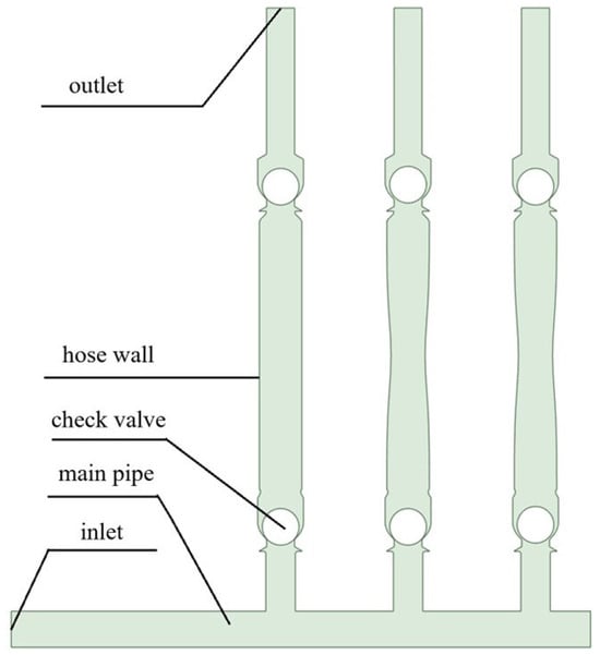
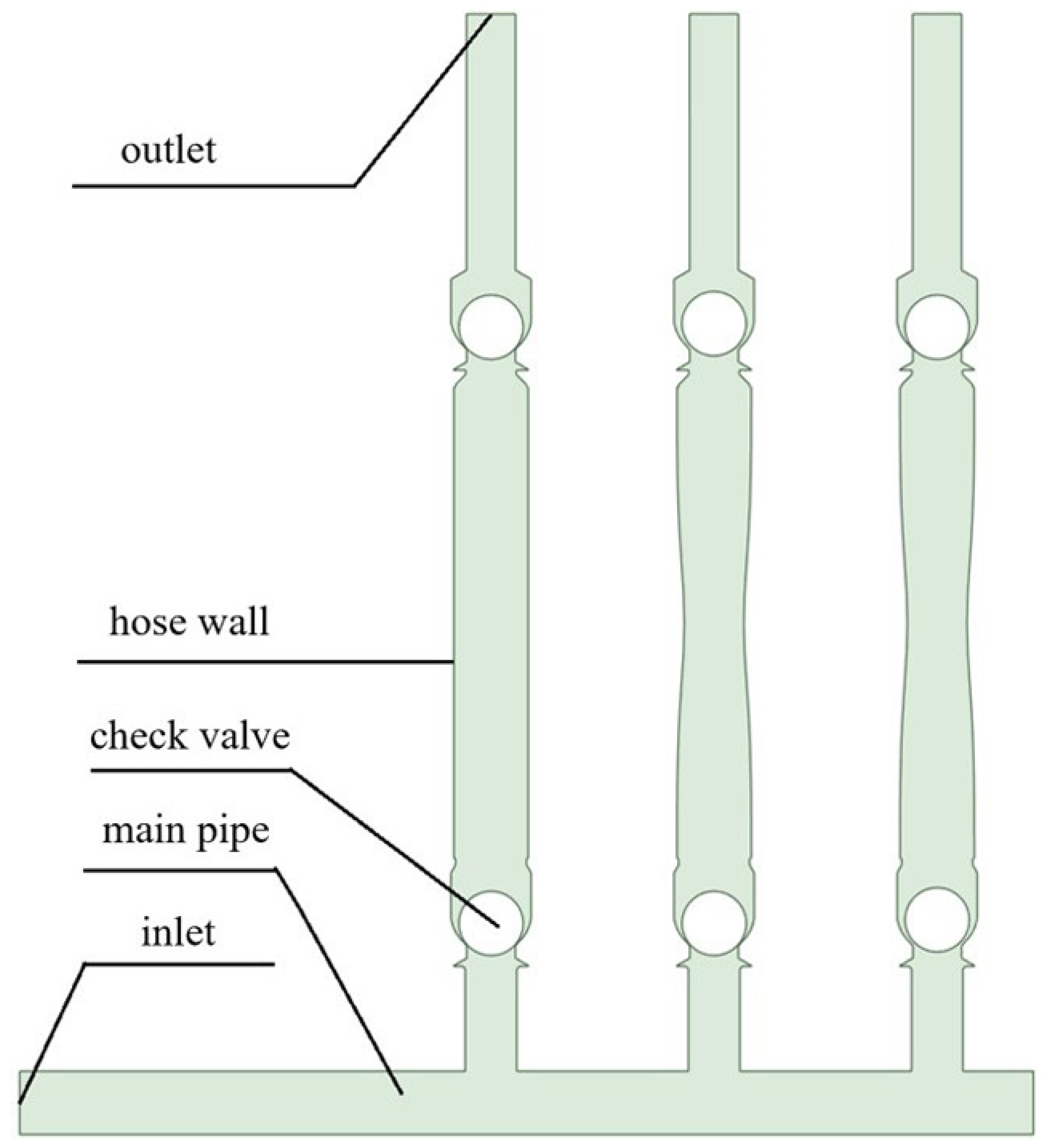
The simplified geometric model used in this study is shown in Figure 1. Based on the CAD front view of the actual pump, the structural characteristics of the internal flow channel are reproduced at equal scale, while the non-core flow-field components, such as the crank–slider mechanism and piston assembly at the power end and the hydraulic oil chamber and diaphragm at the hydraulic end, are removed. Only the key flow-channel structures are retained, including the hose, check valves, inlet and outlet short pipes, and inlet main pipe, with the hose serving as the core active component that drives the flow field. The specific control method of the hose is described in detail in the following sections. The pump unit consists of one inlet main pipe connected in parallel with three diaphragm hose pumps. Each pump chamber is equipped with an inlet check valve and an outlet check valve. The core structure in the middle section of the pump chamber is the hose wall, whose motion is precisely controlled by a user-defined function (UDF).
Figure 1.
Simplified geometric model of the triplex diaphragm pump.
The geometric parameters of the main structures are set as follows: the ball valve diameter is 127 mm; the inner diameter of the inlet and outlet short pipes is 101.5 mm; the inner diameter of the pump chamber (with the hose wall in the vertical position) is 146.5 mm; and the center distance between adjacent pumps is 440 mm.
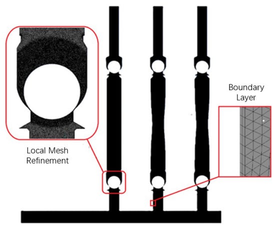
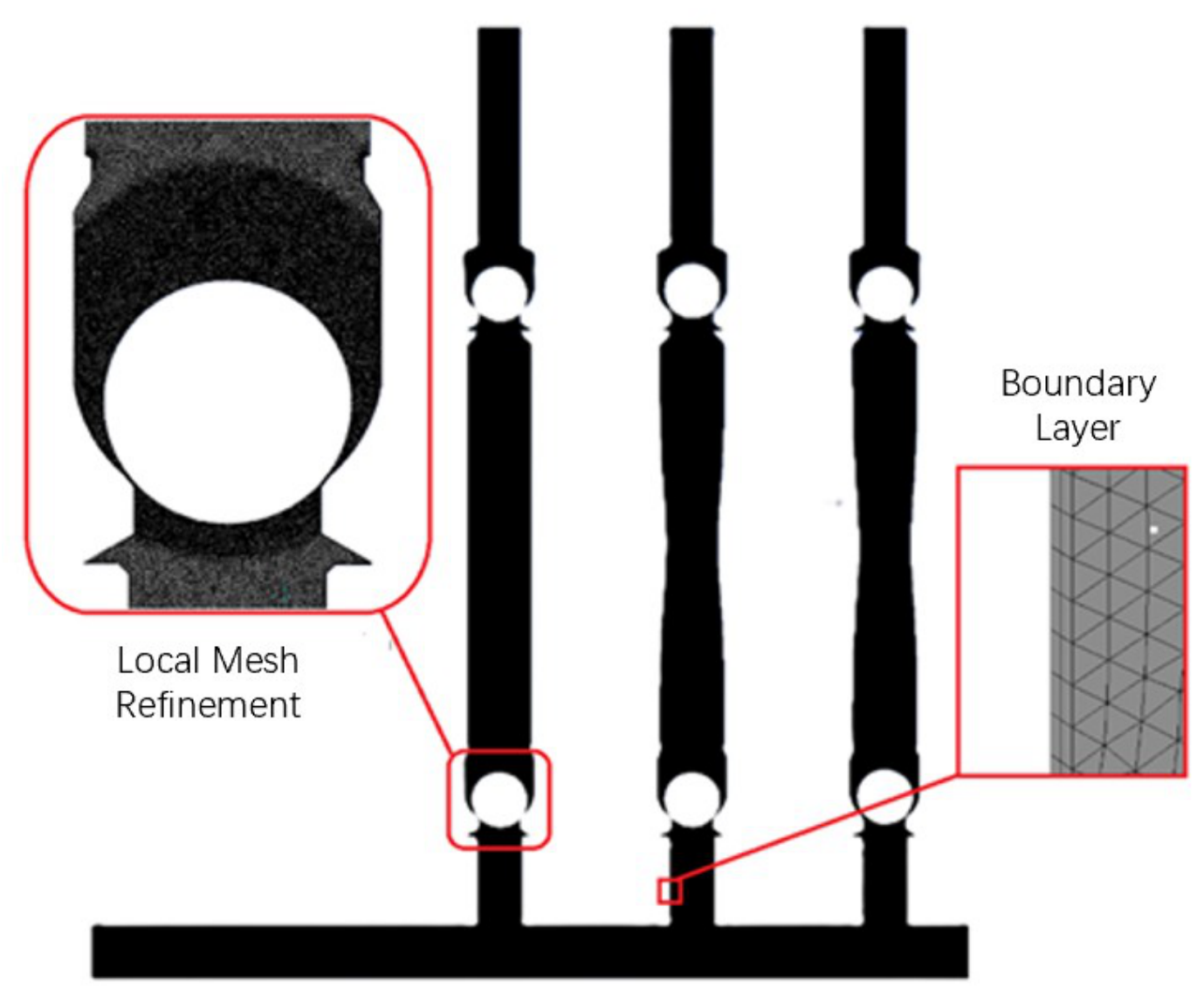
The computational mesh of this study is shown in Figure 2. A hybrid mesh consisting of both structured and unstructured grids is adopted. Structured grids offer high computational accuracy and low computation time, whereas unstructured grids are easy to generate and suitable for geometric models with complex shapes. Specifically, the regular geometric parts of the inlet main pipe and branch pipes are discretized with structured grids dominated by quadrilaterals (hexahedrons), while the moving structures of the check valves and pump chamber accessories are discretized with unstructured hybrid grids dominated by triangles (tetrahedrons).
Figure 2.
Mesh generation for the triplex diaphragm hose pump.
Considering the strong coupling between the ball valve motion and the flow field, and because the valve opening and closing characteristics are key to the normal hydraulic operation of the diaphragm pump, the grid in the valve area is locally refined to accurately capture the flow details. The general grid size is 0.01 m, and the refined grid size is 0.004 m. In addition, boundary-layer grids are added to the walls of the inlet main pipe and each branch pipe to ensure the accuracy of the near-wall flow-field calculation. The boundary layer has 3 layers with a growth rate of 1.15. The dimensionless wall distance obtained from the simulation ranges from 0 to 11.69, which is consistent with the enhanced wall treatment combined with the SST turbulence model adopted in this study, since the enhanced wall treatment is applicable to near-wall cells with values from the viscous sublayer () up to the logarithmic layer (). The final number of grid cells is 330,000, and the average grid orthogonality quality is 0.94704.
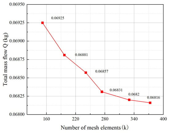
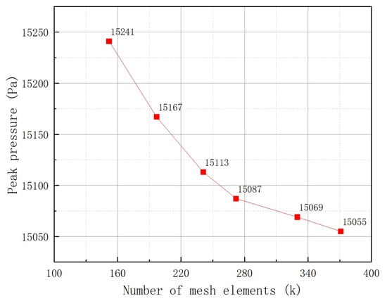
For the grid independence analysis, models with grid numbers of 152,000, 197,000, 241,000, 272,000, 330,000, and 371,000 were compared under the operating conditions of a motor speed of 120 r/min and a hose wall amplitude of m. Two indicators were employed to verify the grid independence: the total mass flow rate within one second (Figure 3) and the peak chamber pressure (Figure 4). As shown in the figures, the total mass flow rate per second decreases with increasing grid number and saturates as the grid is refined; the difference between the 330,000-cell and 371,000-cell meshes is only 0.0004 kg, with a relative error of 0.05%. The peak chamber pressure exhibits a similar monotonic decrease: it drops from 15,241 Pa at 152,000 cells to 15,055 Pa at 371,000 cells, and the difference between the 330,000-cell and 371,000-cell meshes is only 14 Pa, with a relative error of about 0.09%. Both indicators confirm that the 330,000-cell mesh is sufficiently refined. Therefore, 330,000 grids were finally selected for the subsequent numerical simulations, which maintain the highest possible grid quality while reducing memory usage and computational cost to a certain extent.
Figure 3.
Mesh independence analysis based on the total mass flow rate.
Figure 4.
Mesh independence analysis based on the peak chamber pressure.
2.3. Numerical Model Configuration
2.3.1. Solver and Model Settings
The dynamic analysis of the triplex diaphragm hose pump needs to consider various coupling effects and interaction mechanisms: first, the effect of the hose extrusion and contraction on the flow in the pump chamber; second, the coupling effect of the fluid medium in the pump chamber on the ball valve motion; and third, the hydrodynamic interference among the three hose pumps in the inlet main pipe. The foreseeable key technical difficulties in constructing the dynamic simulation model mainly include: precise control of the hose flexural deformation, reasonable simulation of the ball valve opening and closing motion, adaptation of the fluid-domain grid deformation and motion, and effective realization of the coupling between the moving components (hose and ball valve) and the flow-field fluid. These problems need to be addressed and overcome during the model construction and simulation calculation. Considering the incompressible and turbulent nature of the flow, the SST turbulence model is adopted in this study. This model combines the advantages of the model in the near-wall region and the model in the far field, and is therefore well suited to the present pump flow, which involves flow separation and adverse pressure gradients. The enhanced wall treatment is used to resolve the viscous sublayer, which is consistent with the near-wall grid resolution ( up to about 11.69) described in Section 2.2. The numerical simulations are performed with the pressure-based solver in ANSYS Fluent 2022 R1, using liquid water as the working medium and considering the gravitational acceleration of 9.81 m/s2 along the negative y-direction. Since the pump is a positive-displacement pump whose flow is driven by the periodic deformation of the hose wall rather than by an external pressure difference, both the inlet and the outlet boundaries are set as pressure outlets with a relative pressure of 0 Pa, and the operating pressure is 101,325 Pa. For the inlet and outlet pressure boundaries, the turbulence is specified by the Intensity and Hydraulic Diameter method, with a turbulent intensity of 5% and a hydraulic diameter of 125 mm, which corresponds to the characteristic dimension of the inlet manifold. All remaining walls are set as no-slip smooth walls. The time step is 0.0005 s, and the total number of time steps is 10,000. The detailed settings of the CFD model, including the spatial discretization schemes, the pressure–velocity coupling method, and the convergence criterion, are summarized in Table 1.
Table 1.
Summary of the CFD model settings.
Fluid–structure interaction (FSI) is taken into account in this study. The hose wall is treated as an actively moving component whose motion is prescribed in advance, and only the effect of the hose flexural deformation on the internal fluid flow is considered, which corresponds to one-way FSI. In contrast, the interaction between the ball valve and the fluid is two-way FSI: the pressure difference across the ball valve drives the valve motion, and the valve motion reversely changes the geometric boundary of the fluid flow space. In the two-way coupling, the displacement and pressure field data at the ball–fluid interface are transmitted and updated bidirectionally in each iterative calculation to ensure the consistency and accuracy of the solution.
2.3.2. Valve Motion Control
The gap model is a narrow-gap flow control method applied to valves and pumps. When dynamic grids, overlapping grids, or sliding grids are used to simulate the flow in narrow gaps that open or close over time (such as those in valves or rotary pumps), the gap model can block or slow down the flow when the gap is closed. For transient flows with moving surface regions, narrow gaps may open or close within each time step, and the gap model can be used to simulate the flow blockage when the gap is closed.
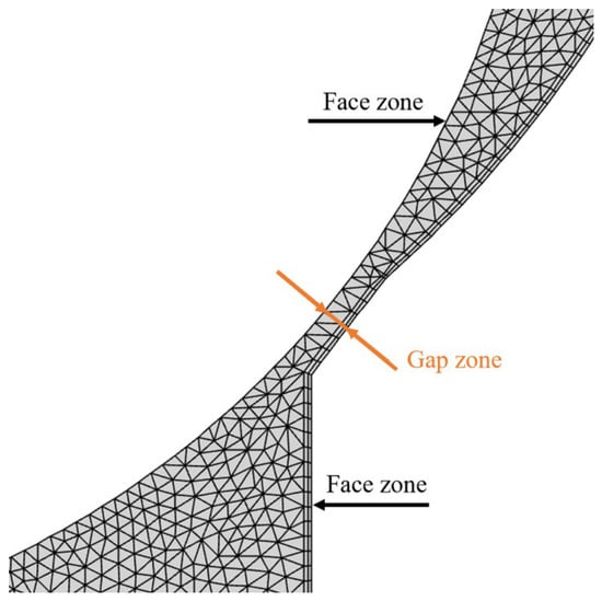
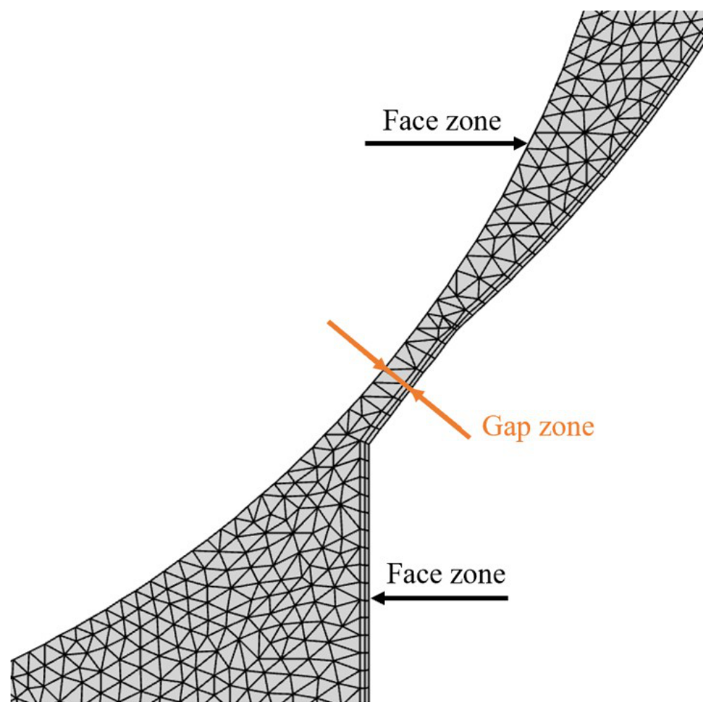
The gap model is applied to a pair of surface regions and the gap region formed between them, as shown in Figure 5. When the distance between the two surface regions reaches the set approach threshold, the fluid cells within the threshold range are marked. The marked fluid cells are then processed differently depending on the selected model. The two gap models are Flow Blocking and Flow Modeling.
Figure 5.
Schematic of the gap model.
Flow Blocking: after selecting this model, zero-mass-flow boundary conditions are applied at the boundary surfaces of the marked fluid cell regions, which completely blocks the flow in the gap region, and the marked cells no longer participate in the solution. This model is more suitable for fully closed valves.
Flow Modeling: this method controls the deceleration of the fluid flow in the marked region cells by adjusting the viscosity parameters or source terms. It allows a small amount of leakage, which can be controlled to a negligible level through reasonable parameter settings, and thus exhibits strong robustness under appropriate parameter configurations. This method is recommended for numerical simulation scenarios with rotating grids, typical examples being the simulation analysis of gears and pump bodies.
The Flow Modeling gap model defaults to a viscosity-based flow control method. By specifying an appropriate gap Reynolds number, the required degree of sealing can be obtained: the lower the gap Reynolds number, the better the sealing effect. The control equation is as follows:
where is the gap Reynolds number; is the average viscosity, in Pa·s; is the average density, in kg/m3; u is the average velocity, in m/s; and L is the approach threshold, in m. Since preliminary tests showed that the fluid leakage with the Flow Modeling gap model could not be ignored, the Flow Blocking model was finally selected in this study. The approach threshold of the gap model is set to 1.9 mm: when the distance between the ball valve and the valve seat becomes smaller than 1.9 mm, the fluid cells within the threshold range are marked and the flow in the gap region is completely blocked, which corresponds to the closed state of the check valve. The approach threshold is chosen such that the gap region can accommodate three layers of grid cells, ensuring that a sufficient number of fluid cells is marked for the Flow Blocking treatment. A smaller threshold would require a finer local mesh, which would increase the cell count and the computational cost while degrading the mesh quality and the accuracy of the results; conversely, an excessively large threshold would cause the model to deviate from the real operating condition of the valve. The adopted value therefore balances the computational accuracy and the fidelity to the actual valve gap.
The motion of the ball valve is controlled by the built-in six-degree-of-freedom (6DOF) solver in Fluent, which calculates the external forces and moments acting on a body undergoing rigid-body motion. These forces are computed by numerical integration of the pressure and shear stress over the body surface. To simplify the calculation, the ball valve is restricted to single-degree-of-freedom translational motion (along the y-axis). The ball valve is a hollow sphere with a mass of 1 kg, and it is allowed to translate along the y-axis within a maximum displacement limit of 7 mm, which simulates the physical valve stopper. At the initial moment, the distance between the ball valve and the valve seat is 1.87 mm, which is smaller than the approach threshold of the gap model (1.9 mm), indicating that the check valve is initially in the closed state. After the center-of-gravity position and the maximum displacement limit of the ball valve are defined, the external forces and displacement of the ball valve are obtained and transmitted to the fluid solver to realize the two-way FSI.
The translational control equation of the center of gravity of the object solved by 6DOF is shown in Equation (4), and the rotational control equation is shown in Equation (5).
where is the acceleration of the center of gravity of the object, in m/s2; m is the mass of the object, in kg; and is the external force vector, in N.
where is the angular acceleration, in rad/s2; L is the inertia tensor, in kg·m2; is the moment vector acting on the object, in N·m; and is the angular velocity vector of the rigid body, in rad/s.
The dynamic mesh model in ANSYS Fluent can simulate flow problems in which the shape of the flow domain changes over time due to the motion of the domain boundary, just as the hose wall, as the fluid-domain boundary in this study, undergoes periodic deformation over time. This dynamic mesh model is applicable to the numerical calculation of single-phase and multi-phase flows. The general transport equation applies to all relevant model equations, including those for turbulence, energy, and phase fields. The motion of the flow-domain boundary can be either prescribed, such as the active flexural deformation control of the hose wall, or non-prescribed, in which the motion state at the next moment is determined from the calculation results at the current moment; for example, computing the velocity and angular velocity according to the force balance of the ball valve through the 6DOF solver.
ANSYS Fluent automatically updates the volume mesh according to the new position of the boundary within each time step. When the dynamic mesh model is used, the user needs to provide the initial volume mesh and define the motion mode of all moving regions in the model. The motion mode can be defined through boundary profiles, user-defined functions (UDFs), or the 6DOF solver.
After the dynamic mesh settings are enabled, for any control volume V with moving boundaries, the conservation equation of the general scalar is as follows:
where is the fluid density; is the flow velocity vector; is the mesh motion velocity; is the diffusion coefficient; is the source term of the scalar ; and denotes the boundary of the control volume V.
Using the first-order difference scheme, the first time-derivative term on the left-hand side of Equation (6) can be written as:
where n and denote the physical quantities at the current and next time steps, respectively. The control volume at time is calculated by:
where is the time derivative of the control volume. To satisfy grid conservation, it is calculated by:
where is the number of faces of the control volume, and is the area vector of the j-th face. The dot product on each control-volume face is obtained by:
where is the volume swept by the control-volume face j in one time step.
2.3.3. Hose Deformation Control
In the actual production process, the hose deformation exhibits significant spatial distribution characteristics: the deformation varies gradually along the radial direction of the hose and is larger closer to the central area. To simplify the simulation model and accurately characterize this experimental observation, a Gaussian distribution function is used in this study to describe the deformation profile of the hose, balancing simulation efficiency and characterization accuracy. This choice is supported by the fluid–structure interaction simulation of a hose pump by Ma et al. [25], in which the total deformation curve of the hose under roller extrusion was shown to be well fitted by a Gaussian function, and it is consistent with the benchmark model of a peristaltic pump in COMSOL Multiphysics 6.1, where the tube-squeezing load is prescribed by a Gaussian distribution along the tube length. The control equation is as follows:
where X denotes the x-coordinate of the element on the hose boundary, which is a function of the y-coordinate y and the time t; is the x-coordinate at the initial moment; T is the period, i.e., the time required for one full rotation of the crank; A is the amplitude; is the y-coordinate of the central element on the hose boundary; and is the width of the Gaussian distribution.
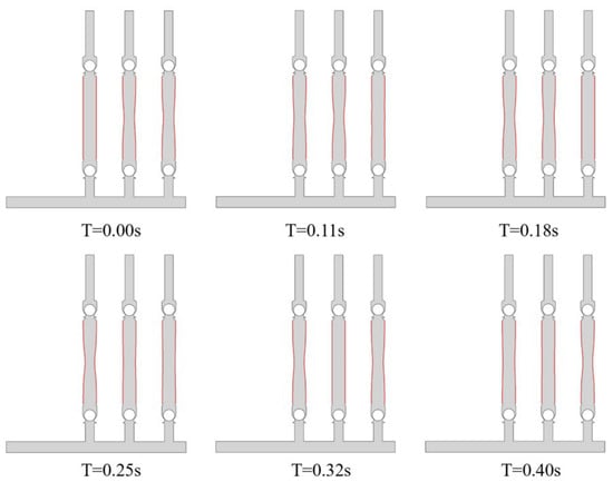
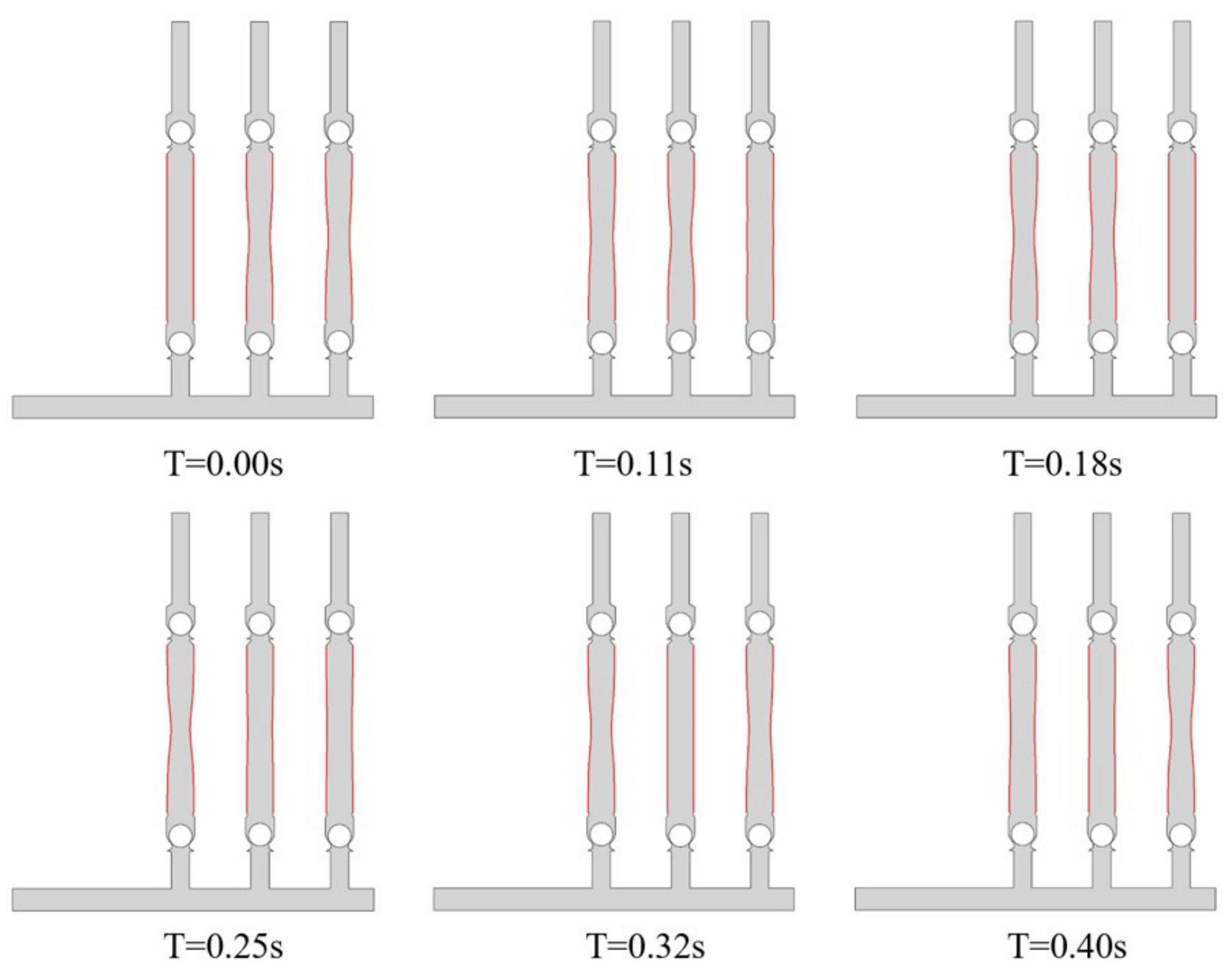
Figure 6 shows the shape of the hose boundary (the thick red curve) at different moments. This study realizes precise control of the boundary deformation and flexure process through a user-defined function (UDF). The dynamic deformation of the hose boundary directly causes periodic contraction and expansion of the fluid domain, thereby driving the fluid flow, which is fully consistent with the working principle of the diaphragm pump. After the compiled UDF program is loaded, the horizontal positions of the hose-wall mesh nodes change dynamically with the simulation time, and their displacement distribution along the y-axis follows the Gaussian distribution law: the mesh cells at the middle of the hose have the largest displacement amplitude, which gradually decreases toward both sides. Meanwhile, the velocity time-history of the hose wall follows the cosine law, and the velocity variation is smooth and stable, without sudden changes or impacts, effectively avoiding the influence of instantaneous excessive acceleration on the calculation stability.
Figure 6.
Hose boundary profiles at different times (period = 0.5 s).
The final deformation is shown in Figure 6. Taking the leftmost pump chamber (pump a) as an example, the boundary gradually undergoes nonlinear bending from the initial straight state ( s) over time, and its flexure continues to increase with time; the deformation reaches its maximum at s, at which time the crank angle of the pump chamber is 180°. Then the hose wall begins to contract and reset toward the initial state, and returns to it at s, completing one cycle of motion.
3. Results and Discussion
3.1. Internal Flow-Field Characteristics of the Pump Under the Baseline Operating Condition
To clarify the internal flow mechanism of the diaphragm pump during stable operation, this section takes the operating condition of a rotational speed of 120 r/min and a hose amplitude of 0.01 m as the research case. Based on the numerical simulation results, the velocity field, pressure field, and vortex structures inside the pump chamber are systematically analyzed. Particular attention is given to revealing the flow characteristics in the suction chamber, discharge chamber, diaphragm motion region, and channel bend sections, as well as identifying the locations and development patterns of unsteady flow phenomena such as flow separation and vortex shedding. This provides a fundamental flow-field basis for subsequent investigations into the effects of different structural parameters and operating conditions on the internal flow field, as well as for hydraulic loss analysis.
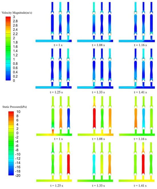
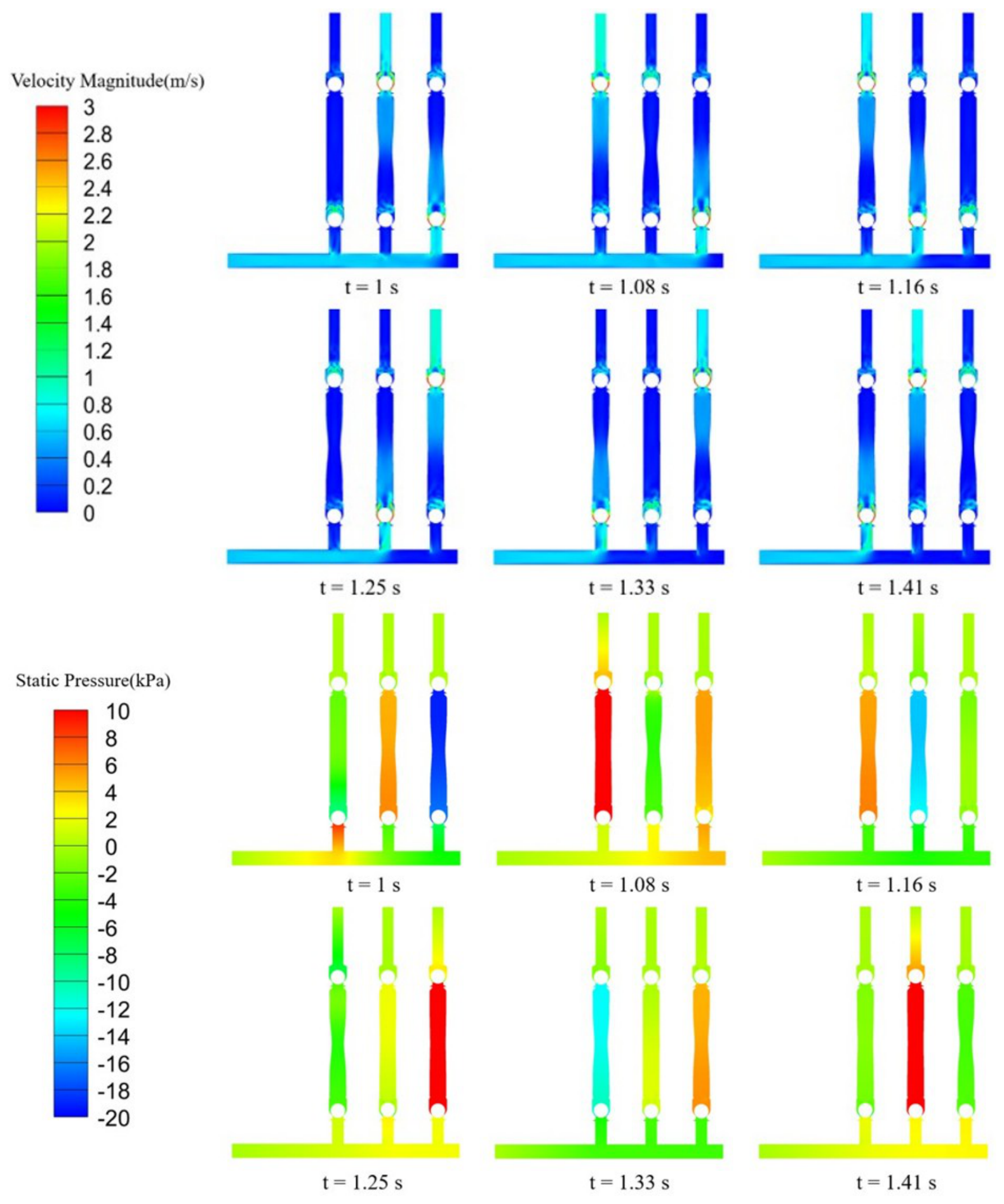
Figure 7 shows the velocity contours (top) and pressure contours (bottom) of the triplex diaphragm hose pump over one complete working cycle, intuitively illustrating the transient evolution of the flow field within the pump chamber. As mentioned earlier, the phase difference among the three pump units is . In this paper, the three pump heads are designated as pump a, pump b, and pump c from left to right, with their flow-rate peaks successively staggered by one-third of a cycle, thereby achieving a stable flow output. Taking the initial moment as an example, pump a is in the transition stage between the discharge stroke and the suction stroke, and both its inlet and outlet check valves are closed, so the theoretical instantaneous flow rate is 0. Pump b is in the discharge stroke, where the hose wall contracts and compresses the fluid inside the chamber, driving the medium toward the outlet. Pump c is in the suction stroke, where the expansion of the hose wall creates negative pressure inside the chamber, causing the fluid to flow in from the inlet.
Figure 7.
Transient evolution of the velocity contours (top) and pressure contours (bottom) in the triplex diaphragm hose pump during one complete working cycle.
From the pressure contours, it can be clearly observed that a diaphragm pump in the discharge stroke (such as pump b at ) exhibits a significantly higher pressure inside the pump chamber than at the inlet and outlet, thereby forming a high-pressure region. In contrast, the diaphragm pump in the suction stroke (such as pump c at ) has a chamber pressure markedly lower than that at the inlet and outlet, resulting in a low-pressure region. With the ball valve as the boundary, a pronounced pressure gradient exists across its upper and lower sides, providing the primary driving force for the opening and closing of the ball valve. Meanwhile, during the rapid valve-closing process, owing to the inertia effect of the fluid, a transient positive-pressure region forms upstream of the ball valve, while a corresponding low-pressure region appears downstream. This pressure difference is an important cause of the ball rebound phenomenon.
The working state of each branch pipe can also be clearly identified from the velocity distribution in the inlet manifold: the inlet velocity of the branch pipe in the suction stroke is significantly higher than that of the other branch pipes. As the fluid flows from the manifold into the branch pipe, an evident low-velocity region forms on the inner side of the bend, and the area of this region increases as the distance between the branch pipe and the inlet pipe decreases. This directly reflects the occurrence of flow separation at the junction between the manifold and the branch pipe. In addition, as the fluid passes around the ball, boundary-layer separation occurs, forming a local vortex structure downstream of the ball valve. This vortex possesses a certain degree of inertia; even after the check valve is fully closed, it persists for some time before gradually dissipating.
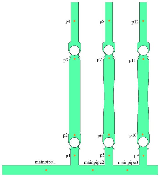
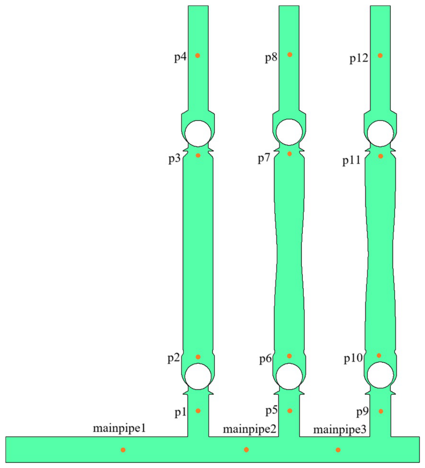
In this study, several monitoring points were arranged to record flow-field parameters for auxiliary analysis of the flow characteristics, as shown in Figure 8. Three monitoring points were located in the inlet manifold and were designated as mainpipe1, mainpipe2, and mainpipe3 from left to right. Moreover, four monitoring points were arranged for each diaphragm pump and its corresponding inlet and outlet pipes. For pump a, these points were designated as p1, p2, p3, and p4 from bottom to top, and the same designation method was adopted for pumps b and c.
Figure 8.
Locations of the monitoring points in the triplex diaphragm hose pump.
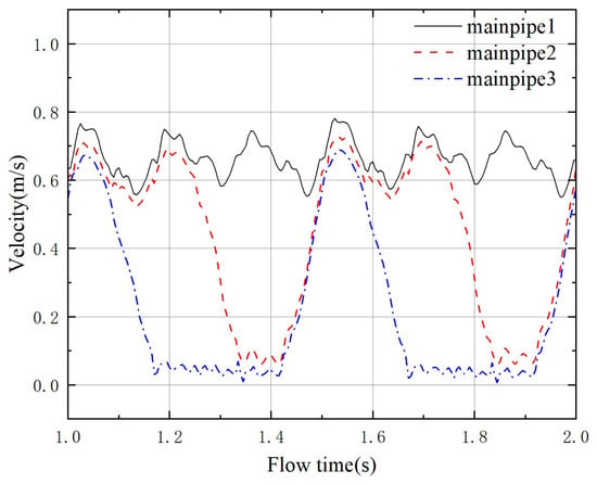
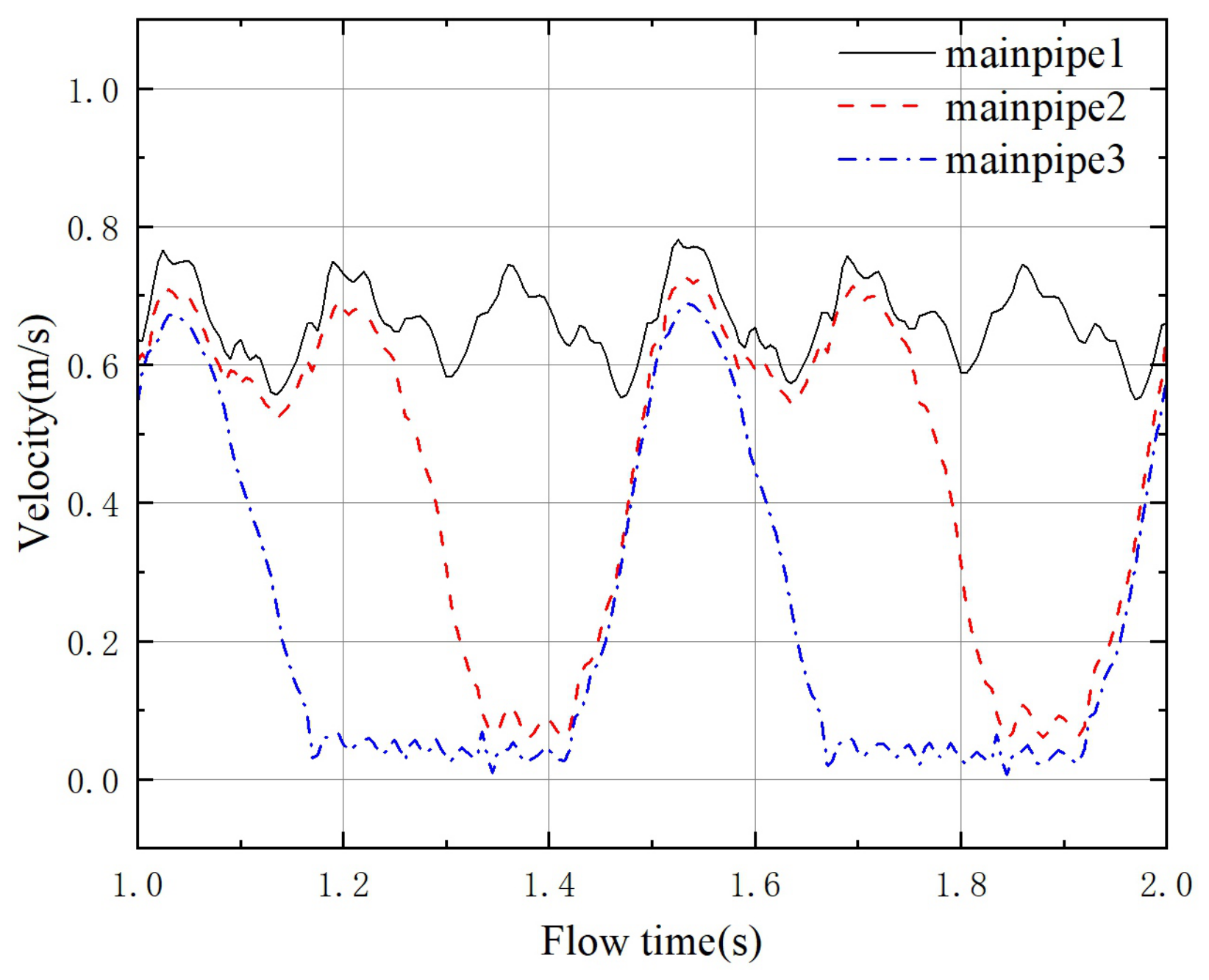
Figure 9 presents a lateral comparison of the flow velocities at the three monitoring points in the manifold. The velocity at mainpipe3 exhibits only local fluctuations during the suction stroke of pump c and remains close to 0 m/s at all other times. The velocity at mainpipe2 shows local fluctuations only during the suction strokes of pumps b and c, whereas the velocity at mainpipe1 remains within the range of 0.57–0.78 m/s throughout the cycle. Moreover, its peak values are synchronized with the instants of maximum instantaneous flow rate during the suction strokes of each pump head. The peak corresponding to the suction stroke of pump c is greater than those corresponding to the suction strokes of the other two pumps, with a difference of approximately 0.05–0.10 m/s. This difference reflects the variation in the disturbance intensity imposed on the manifold flow field by the suction and discharge timing of different pump units.
Figure 9.
Lateral comparison of the flow velocities at the three monitoring points in the manifold.
Taking the velocity distribution at as an example, pumps a and b are in the discharge stroke, while pump c is in the suction stroke. At this moment, the velocity at mainpipe1 is about 0.78 m/s, that at mainpipe2 is about 0.72 m/s, and that at mainpipe3 is about 0.68 m/s, indicating that the spatial distribution of flow velocity in the manifold gradually decreases from left to right. This gradient distribution mainly arises from the energy dissipation caused jointly by frictional resistance along the pipe, local disturbances, and boundary-layer development during the flow process, resulting in a gradual attenuation of fluid kinetic energy and, consequently, a reduction in flow velocity along the flow direction.
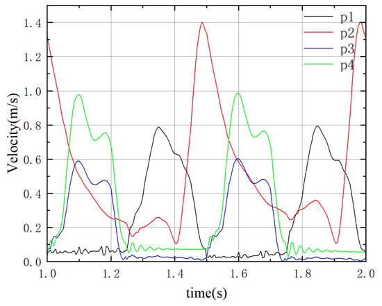
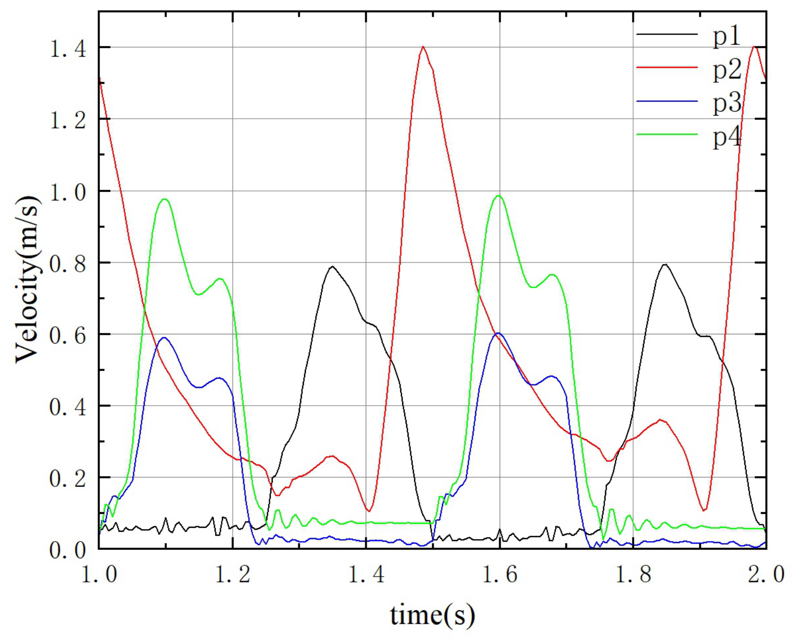
Figure 10 shows the longitudinal comparison curves of the flow velocities at the four monitoring points of pump a. Points p3 and p4 are located upstream and downstream of the outlet valve, respectively, and their velocity curves exhibit generally similar variation trends. During the discharge stroke, the velocity curves show significant fluctuations with two secondary peaks. The peak velocity at point p3 is close to 0.58 m/s, while that at point p4 is close to 0.98 m/s. The higher velocity at point p4 than at point p3 can be attributed to the fact that the inner diameter of the pump chamber is larger than that of the outlet branch pipe, causing the fluid velocity to increase as it flows through the outlet branch pipe.
Figure 10.
Longitudinal comparison curves of the flow velocities at the four monitoring points of pump a.
The velocity curve at point p1 changes significantly during the suction stroke (1.0–1.25 s), whereas during the discharge stroke (1.25–1.5 s) the velocity remains basically around 0 m/s, which is consistent with the theoretical expectation. The variation characteristics of the velocity curve at point p2 differ markedly from those at the other three points, with a larger fluctuation amplitude and a peak velocity reaching 1.38 m/s. Overall, the velocity at point p2 decreases rapidly from a high level at the beginning of the discharge stroke, then declines more gradually during the middle stage of the discharge stroke. This trend continues until the middle of the suction stroke, where the velocity reaches its minimum value. In the second half of the suction stroke, the velocity begins to rise sharply and reaches its peak before the end of the suction stroke.
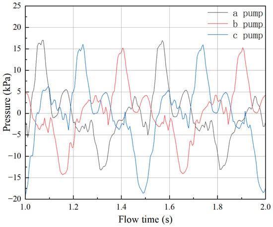
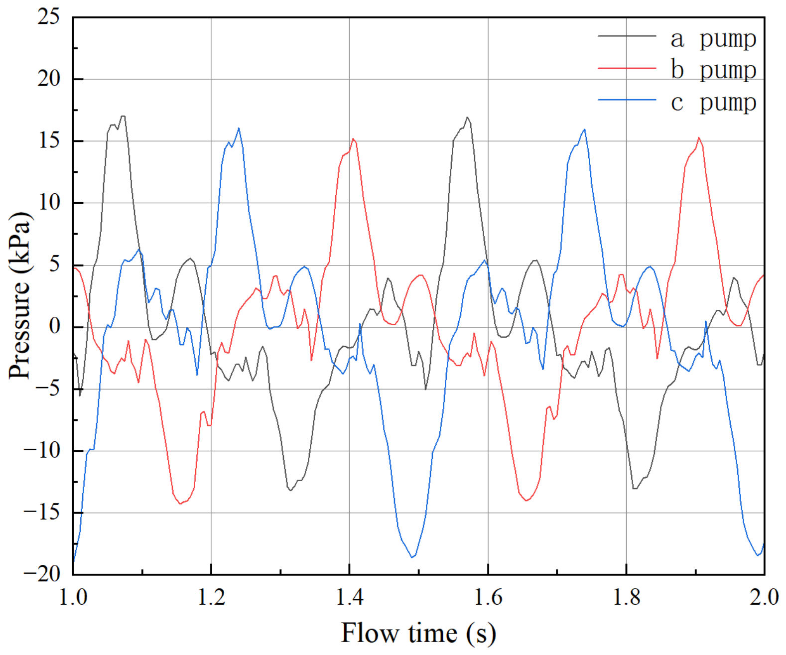
Figure 11 compares the chamber pressures of the three pumps. Within a single operating cycle, the chamber-pressure response curves exhibit generally similar trends, with only small differences in the peak values, all of which are around 15 kPa. The peak pressures are ranked in descending order as pump a > pump c > pump b. In contrast, the minimum pressure of pump c is significantly lower than those of the other two pumps, reaching about kPa, whereas the minimum pressures of pumps a and b are both around kPa.
Figure 11.
Comparison of the chamber pressures of the three pumps during one operating cycle.
Overall, during the discharge stroke, the chamber pressure of each pump head first rises rapidly to a peak value and then fluctuates downward to the range of to 5 kPa. During the suction stroke, the opposite trend is observed: the chamber pressure first drops rapidly to a minimum value and then fluctuates upward to the range of to 5 kPa. It is worth noting that the peak points of the temporal response curves of the chamber pressure for the three pumps almost coincide with the moments when one pump switches from the discharge stroke to the suction stroke. For example, the flow instant corresponding to the chamber pressure peak at point p3 (pump a) is 1.585 s, while pump b switches from the discharge stroke to the suction stroke at 1.583 s. Similarly, the moments corresponding to the minimum values of the pressure curves nearly coincide with the time points when one pump finishes the suction stroke and begins the discharge stroke.
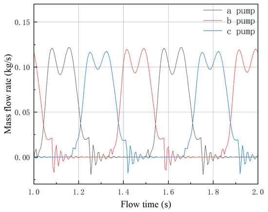
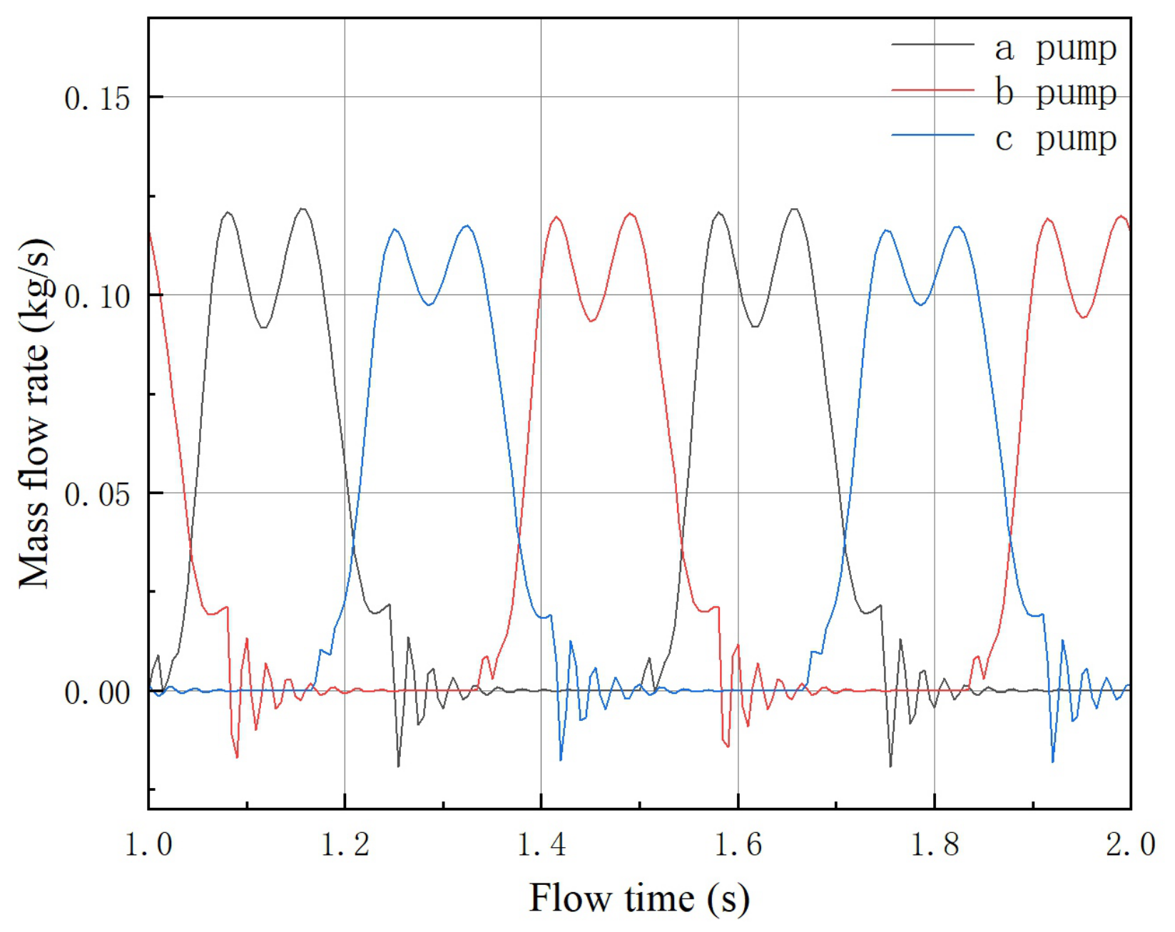
Figure 12 presents the temporal response curves of the outlet mass flow rates of pumps a, b, and c. The mass flow rate curves of the three pumps exhibit pronounced common features: all of them show periodic pulsations highly synchronized with the suction–discharge cycle, and during the discharge stroke, the flow-rate curves all display a typical “double-peak–single-valley” pattern. Specifically, the flow rate first rises rapidly to the first peak, then decreases briefly to form a valley, rises again to the second peak, and finally drops rapidly to nearly 0 kg/s at the end of the discharge stroke, accompanied by small oscillations. At this stage, the instantaneous outlet mass flow rate may become negative, indicating the occurrence of outlet backflow. In addition, the peak flow rates of the three pumps are staggered in time, thereby forming an alternating discharge mode.
Figure 12.
Temporal response curves of the outlet mass flow rates of pumps a, b, and c.
At the same time, differences can also be observed among the flow-rate curves of the three pumps. Pump a exhibits the highest peak values and the lowest valley values, with a peak flow rate of about 0.12 kg/s and a valley value as low as about 0.02 kg/s. In contrast, pump c shows the lowest peak values and the highest valley values, with a peak flow rate of about 0.10 kg/s and a valley value of about 0.04 kg/s. The peak and valley values of pump b lie between those of pumps a and c.
Figure 13 shows the cumulative conveyed mass curves obtained by integrating the instantaneous mass flow-rate curves of pumps a, b, and c. By jointly examining the monitoring data in Figure 12 and Figure 13, it can be found that pump a, which is closest to the inlet, exhibits the highest peak mass flow rate, whereas its total cumulative conveyed mass within 1 s (two working cycles) is the smallest, at approximately 0.02258 kg. In contrast, pump c, which is farthest from the inlet, has the lowest peak mass flow rate, while its total cumulative conveyed mass within 1 s reaches 0.02283 kg. The performance indicators of pump b lie between those of pumps a and c, whereas its total cumulative conveyed mass within 1 s is the largest, at approximately 0.02299 kg. Based on these differences, it may be inferred that, under the influence of the flow-channel structure, the actual operating flow rates of the three pumps become unbalanced, thereby giving rise to a flow-field characteristic similar to “water grabbing”, which causes an inverse relationship between the cumulative conveyed mass and the peak flow rate of each pump.
Figure 13.
Cumulative conveyed mass curves of pumps a, b, and c obtained by integrating the instantaneous mass flow-rate curves.
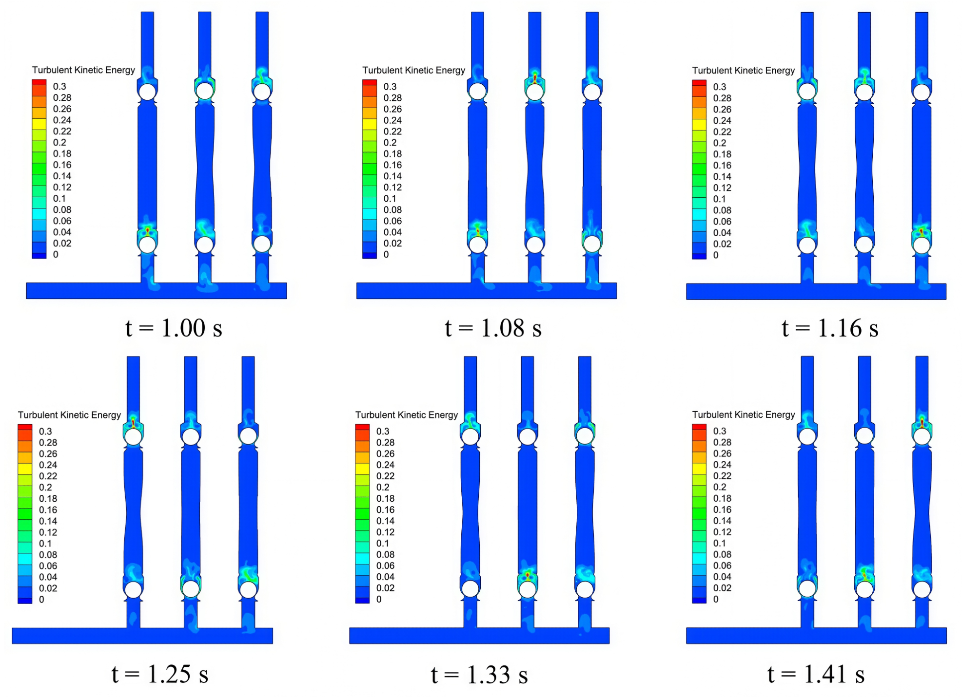
Figure 14 presents the contour distributions of the turbulent kinetic energy K in the triplex diaphragm hose pump at multiple instants. It can be seen that the distribution of turbulent kinetic energy exhibits pronounced localization and periodicity. Regions of high turbulent kinetic energy are mainly concentrated near the inlet and outlet valves and around the pump chamber, whereas the turbulence level in the main flow region and the manifold remains generally low. At different instants, the high-K regions (0.1–0.5 ) are all located near the valve ports. This is because intense shear and flow separation occur during valve opening and closing, generating strong vortex structures and thus high turbulence levels. In contrast, in most areas of the pump chamber and branch pipes, the turbulent kinetic energy remains at a relatively low level (<0.1 ).
Figure 14.
Contour distributions of turbulent kinetic energy K in the triplex diaphragm hose pump at different instants.
From the perspective of temporal evolution, the turbulent kinetic energy distribution is closely related to the motion of the ball valve. When the valve rises and the flow passage has just opened, the fluid passes at high speed through the narrow gap between the ball and the valve seat, forming intense shear turbulence, followed by flow separation after passing along both sides of the ball. When the valve reaches its maximum lift and the flow passage is fully open, the turbulent structures continue to develop along the pipe wall toward the narrowed passage outlet. As the ball begins to fall back, the turbulent flow gradually converges toward the middle of the passage and forms vortices. At this stage, the turbulent kinetic energy at the centered region above the check valve increases significantly (>0.25 , accompanied by an increase in flow velocity. After the valve is fully closed, the flow disturbance gradually weakens, and the turbulence correspondingly dissipates, thus completing one full periodic evolution process.
As the core flow passage for the parallel operation of the triplex pump, the diameter of the inlet manifold is directly related to the pressure distribution in the main pipeline and thus determines whether the flow can be evenly distributed. Meanwhile, the operating flow rate, as a key process parameter, is not only related to the actual conveying efficiency of the pump, but also alters the internal flow state and the development characteristics of turbulence. Both factors have important effects on the internal pressure distribution, flow pulsation, turbulent kinetic energy evolution, and the stability of ball-valve motion. In the following sections, the inlet manifold diameter and the operating flow rate are taken as the main variables, and a series of numerical simulation tests are carried out using the controlled-variable method. The aim is to systematically investigate the differences in the internal flow-field distribution under different manifold diameters and operating flow conditions, and to analyze their effects on the internal velocity and pressure distributions, flow pulsation characteristics, turbulent kinetic energy evolution, and flow distribution uniformity, thereby providing a theoretical basis for the subsequent operating-condition regulation of the triplex diaphragm hose pump.
3.2. Effect of Operating Flow Rate on the Internal Flow Field of the Pump
For a single operating cycle, the discharge volume of the diaphragm pump is determined by the product of the piston cross-sectional area and the piston stroke. Since the piston component is neglected in the present simplified model and the bending deformation of the hose wall is directly imposed, the volumetric change in the pump chamber over one cycle can be written as Equation (12):
where V is the volumetric variation of the pump chamber during one operating cycle, in ; A is the amplitude of the hose wall following a Gaussian distribution, in ; is the thickness of the geometric model in the 2D case, which is fixed at 1, and its unit is consistent with the length unit defined in the simulation setup, which is in the present study; and , , and are the vertical coordinates of the center point, highest point, and lowest point of the hose wall, respectively. It can be seen from Equation (12) that, with all other parameters kept constant, the flow rate of the diaphragm pump is linearly related to the hose-wall amplitude A. Therefore, in this study, the amplitude parameter A is selected as the independent variable, and the pump flow rate is regulated by varying the amplitude, so as to systematically investigate the influence of flow-rate variation on the internal flow characteristics of the pump.
Eight cases with different hose-wall amplitudes were selected for data analysis in this study. The first aspect examined was the relationship between the area-weighted average instantaneous velocity in the inlet manifold and the hose-wall amplitude A. Under different hose-wall amplitudes, no significant difference was observed in the characteristics of the temporal response curves of velocity. The statistical characteristics of the temporal velocity response curves are summarized in Table 2. It can be seen from the table that, as the hose-wall amplitude (i.e., the operating flow rate) increases, the velocity in the inlet manifold also increases correspondingly. Moreover, the average velocity over a single cycle exhibits a good positive linear correlation with the hose-wall amplitude, which is expected from the volume-displacement mechanism described by Equation (12), whereas the standard deviation and range of the curves are only slightly affected by the hose-wall amplitude and remain fluctuating within a limited interval.
Table 2.
Statistical characteristics of manifold velocity under different flow rates.
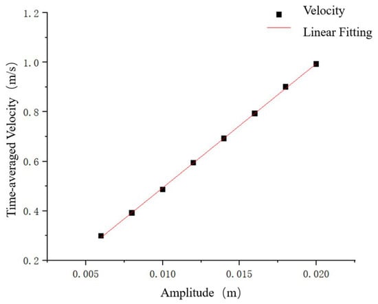
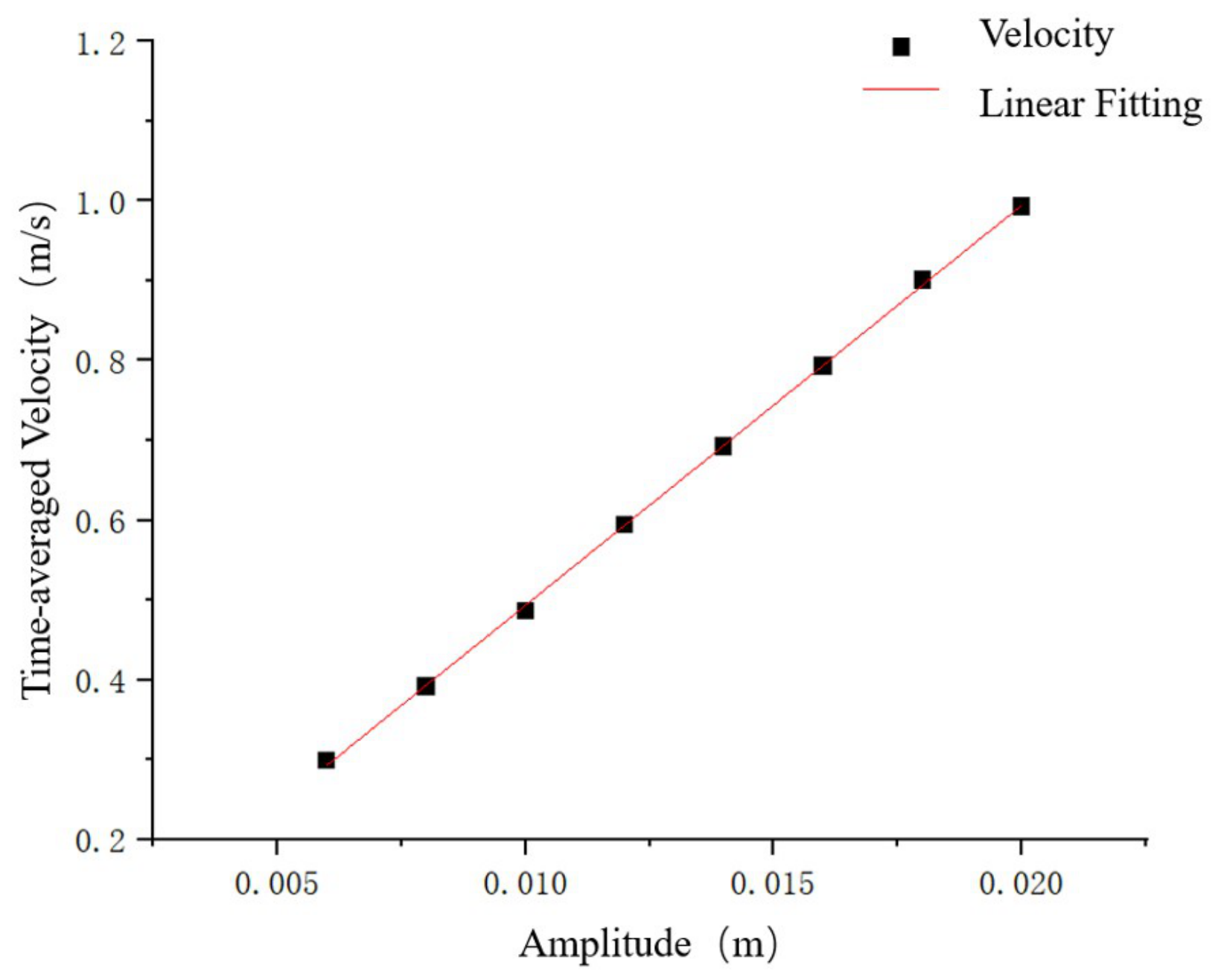
Figure 15 shows the linear fitting curve of the mean velocity in the manifold over one operating cycle. Within the investigated amplitude range of 0.005–0.020 m, the mean velocity increases monotonically and linearly with the hose amplitude A, with the scattered data points fitting the regression line closely. This linear relationship is an expected result: as shown in Equation (12), the chamber volume change over one operating cycle is approximately proportional to the amplitude, and the resulting displacement flow rate consequently scales linearly with A. Therefore, this aspect is not discussed further, and the remainder of this subsection focuses on the pressure pulsation and the normalized flow pulsation, which are of greater relevance to the reliability and operational stability of the pump system.
Figure 15.
Linear fitting curve of the mean velocity in the pipe under different amplitudes.
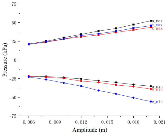
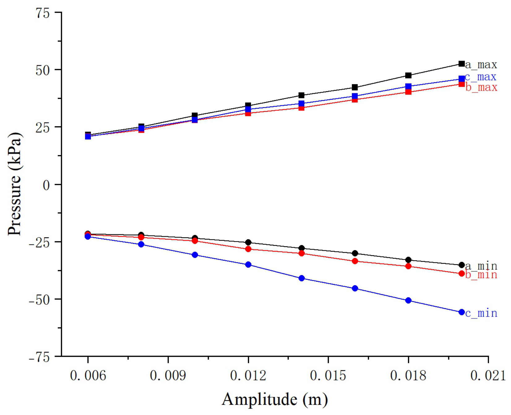
In contrast to the mean velocity, whose linear variation with the amplitude is an expected consequence of the volume-displacement mechanism, the pressure pulsation is a more meaningful indicator of the pump operating state and reliability. Figure 16 shows the variations in the maximum and minimum chamber pressures of the three pumps with the amplitude A. As can be seen from the figure, both the maximum and minimum chamber pressures of each pump exhibit monotonic trends with increasing amplitude A: the maximum pressure increases, whereas the minimum pressure decreases, indicating that an increase in the flow rate significantly intensifies the chamber-pressure pulsation.
Figure 16.
Variations in the maximum and minimum chamber pressures of the three pumps with hose-wall amplitude A.
In terms of the maximum chamber pressure, pump a always exhibits the highest value, followed by pump c, while pump b shows the lowest value. In contrast, for the minimum chamber pressure, pump c always has the lowest value, followed by pump a, whereas pump b has the highest value. This regular pattern is closely related to the positions of the three pumps in the manifold. Overall, as the amplitude A increases, the pressure fluctuation range of all three pump chambers expands significantly. This implies that increasing the flow rate not only enhances the conveying capacity of the pump, but also aggravates the alternating pressure variation inside the chamber, which may have important implications for the fatigue life and operational stability of the pump structure.
In addition to velocity and pressure, the temporal response characteristics of the total instantaneous mass flow rate of the system are also a key focus of this study. Its peak value, valley value, and pulsation rate directly determine the intensity of flow pulsation and the level of alternating load in the system. Excessively high peak and valley values may aggravate the fatigue damage of pipes and valves, while a large pulsation rate may reduce the operational stability of the system. Therefore, an in-depth analysis of these characteristics is essential for evaluating the reliability and service life of the pump system.
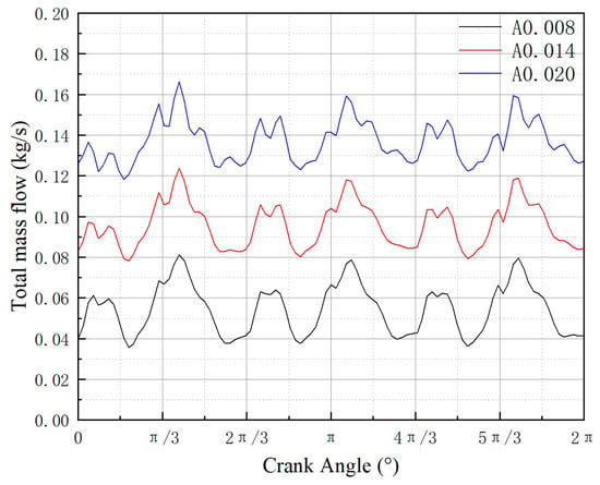
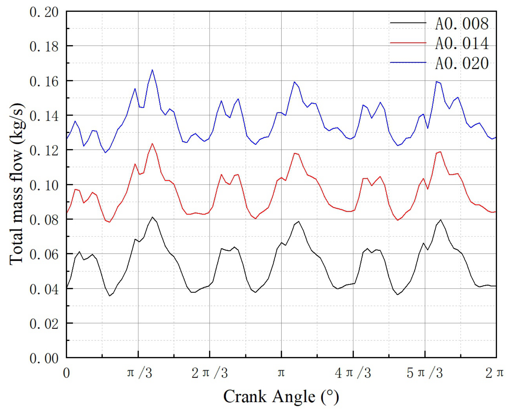
Figure 17 shows the variation of the total instantaneous mass flow rate in the manifold with crank angle under three typical amplitude conditions. It can be seen from the figure that the overall level of the total instantaneous mass flow rate in the manifold is significantly positively correlated with the amplitude, and three groups of periodic peaks appear within the crank-angle range of 0–2. The overall evolution trends of the curves under different operating conditions are highly consistent. However, differences can still be observed in the curve shapes under different conditions: as the flow rate increases, the total instantaneous mass flow-rate curve gradually changes from a relatively smooth profile to one with stronger local fluctuations, indicating that the local characteristics of flow pulsation become more pronounced under high-flow-rate conditions.
Figure 17.
Temporal variations of the total instantaneous mass flow rate in the manifold with crank angle under three typical amplitude conditions.
To quantitatively characterize the flow-pulsation characteristics under different operating conditions, two normalized pulsation rates, and , are defined. From the total instantaneous mass flow-rate curve, the cycle-averaged mass flow rate (defined as , which is the time average over one working cycle rather than the arithmetic mean of the sampled data), the maximum mass flow rate , and the minimum mass flow rate are first extracted. The two pulsation rates are then defined as:
These two metrics are introduced because the upper amplitude and the lower amplitude of the instantaneous flow rate of a positive-displacement pump are generally not equal; therefore, using the absolute range alone cannot fully reflect the asymmetric pulsation characteristics of the flow. The calculated results show that, under the condition, the difference between the maximum and minimum amplitudes is , the flow pulsation rate is , and the flow pulsation rate is ; under the condition, , , and ; under the condition, , , and .
From the above data, it can be concluded that although the range of the instantaneous mass flow rate shows a slight increasing trend with increasing flow rate, its growth is not significant relative to the overall level of the instantaneous mass flow rate. Therefore, the normalized flow pulsation rates and exhibit an inverse decreasing trend as the flow rate increases, indicating that within the operating range considered in this study, although the increase in flow rate enlarges the absolute pulsation amplitude, the flow-pulsation characteristics of the system are actually improved to a certain extent from the perspective of relative pulsation intensity.
3.3. Effect of Inlet Manifold Diameter on the Internal Flow Field of the Pump
The manifold diameter is a core structural parameter of the flow-passage system in the triplex diaphragm pump. Its design size directly determines the uniformity of flow distribution within the pump, the stability of the flow field, and the feasibility of engineering application. Both excessively large and excessively small manifold diameters have evident drawbacks. When the manifold diameter is excessively large, the flow cross-sectional area increases and the flow velocity decreases, which can weaken flow inertia and local disturbances and thus alleviate the nonuniform flow distribution caused by positional differences among multiple pump heads. However, this also increases material consumption and manufacturing cost. In addition, installation-space limitations may reduce the engineering adaptability of the equipment. When the manifold diameter is too small, the flow capacity becomes insufficient and the flow velocity in the manifold becomes excessively high, which intensifies the flow interference among the branch pipes of different pump heads. This aggravates nonuniform flow distribution, flow separation, and local vortex formation, leading to pressure and flow-rate pulsations, reduced synchronization among pump heads, and decreased operational stability of the system. At the same time, it increases flow resistance and energy loss in the passage, thereby weakening the conveying efficiency of the pump.
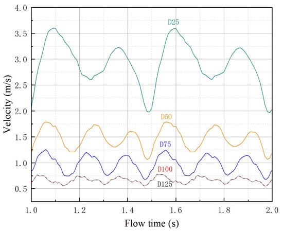
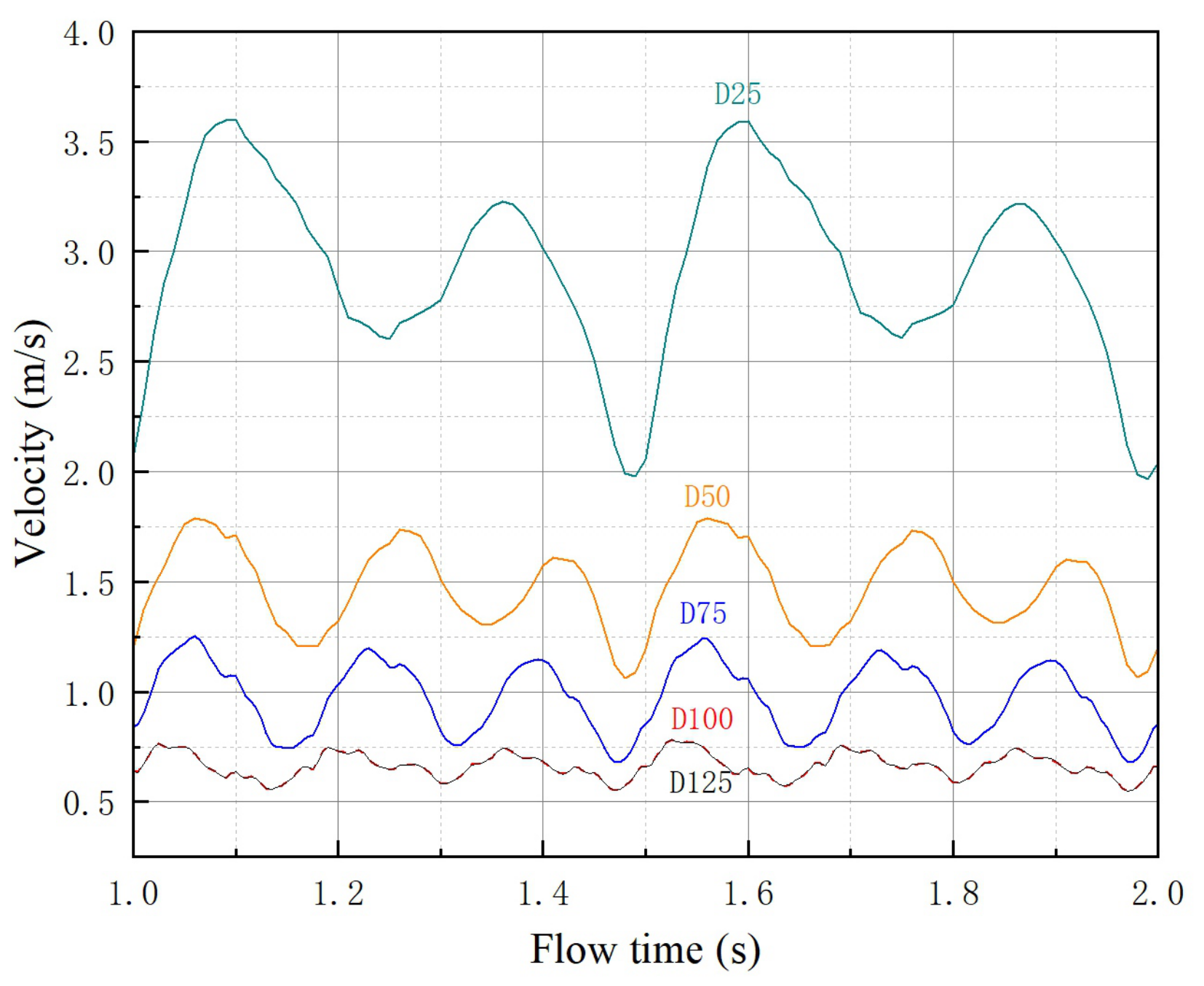
Figure 18 shows the temporal response curves of the flow velocity in the manifold under different inlet-manifold diameters. It can be seen from the figure that, except for the D25 condition, the velocity curves under the other diameter conditions all exhibit periodic pulsation characteristics synchronized with the working cycle of the triplex diaphragm pump. In contrast, the velocity evolution under the D25 condition shows a distinctly different pattern: the number of pulsation peaks is smaller, the phase shift is obvious, and the velocity amplitude is much higher than those under the other diameter conditions. The peak velocity reaches approximately 3.6 m/s, which is more than five times that under the D125 condition. This indicates that, under the small-diameter condition, the coupling effect of the fluid inertia and the flow-passage resistance significantly alters the flow characteristics inside the manifold. As the diameter gradually increases from D50 to D125, the velocity amplitude decreases in a stepwise manner, and the pulsation curves become progressively smoother. This demonstrates that increasing the manifold diameter can effectively weaken fluid inertia effects and reduce flow-passage resistance, thereby suppressing the amplitude of velocity pulsation and making the flow state more stable.
Figure 18.
Temporal response curves of the flow velocity in the inlet manifold under different manifold diameters.
Table 3 summarizes the statistical characteristics extracted from the velocity curves in Figure 18, providing a more intuitive comparison. In terms of velocity magnitude, the manifold velocity is clearly negatively correlated with the manifold diameter. Under the D25 condition, the peak velocity is the highest, reaching approximately 3.6 m/s, and the mean velocity is also significantly higher than those under the other conditions. As the diameter increases successively to D50 and D75, both the peak velocity and the mean velocity decrease in a stepwise manner. It is worth noting that the velocity curves under the D100 and D125 conditions almost completely overlap, indicating that once the diameter increases to D100, the regulating effect of further increasing the diameter on the manifold velocity becomes saturated, and the velocity level no longer decreases significantly with increasing diameter. This phenomenon is consistent with the continuity equation, namely that when the diameter increases to a certain extent, the marginal effect of further enlargement of the flow cross-sectional area on the flow velocity becomes negligible.
Table 3.
Statistical characteristics of manifold velocity under different manifold diameters.
From the perspective of pulsation intensity, the velocity fluctuation is more severe under small-diameter conditions. Under the D25 condition, not only is the peak velocity high, but the peak-to-valley difference is also large, and the curve exhibits obvious undulations. As the diameter increases, the peak-to-valley range of the velocity gradually decreases, and the curve shape becomes smoother. Under the large-diameter conditions of D100 and D125, the velocity pulsation amplitude is significantly attenuated, and the curves become nearly stable. This indicates that a larger diameter effectively weakens the flow-pulsation effect induced by the alternating suction and discharge of the pump heads, thereby improving the flow stability inside the manifold.
Mass flow rate is a key monitoring parameter of the triplex diaphragm pump system. The main focus of the analysis includes both the temporal response curves of instantaneous mass flow rate and the cumulative mass flow rate per unit time. The instantaneous mass flow-rate curves can be used to extract flow characteristics such as flow-rate extrema and pulsation rate, whereas the cumulative mass flow rate per unit time can serve as an important basis for analyzing the differences in operating conditions among the pump heads.
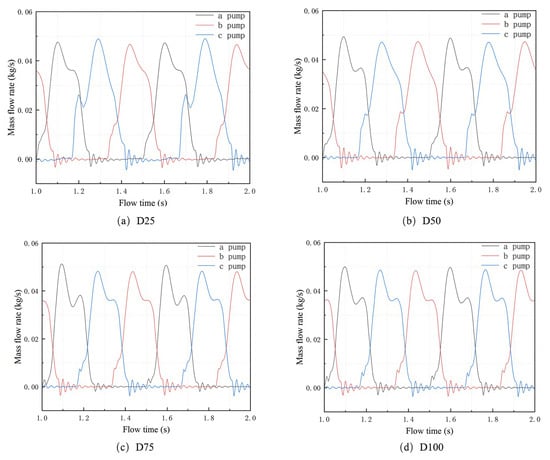
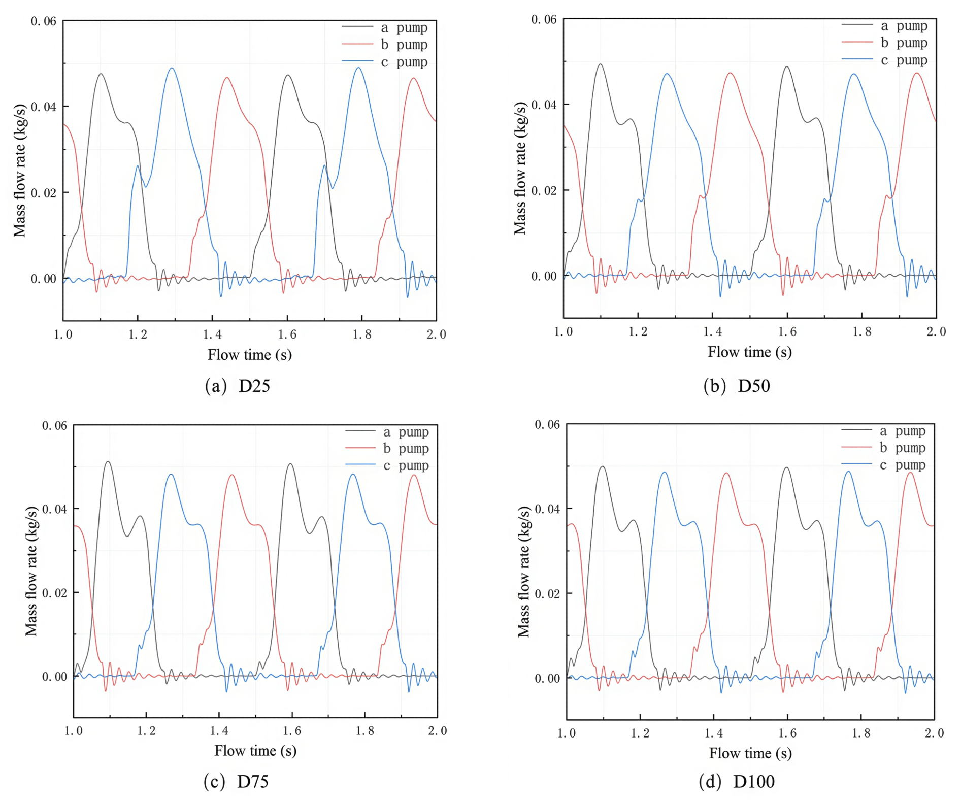
Figure 19 shows the temporal response curves of the instantaneous outlet mass flow rates of the three pump heads in the triplex diaphragm hose pump under different manifold-diameter conditions. As can be seen from the figure, the responses of the outlet mass flow-rate curves of the pump heads to changes in the manifold diameter differ significantly. Specifically, the instantaneous outlet mass flow-rate curves of pump a remain relatively consistent under different diameter conditions, indicating that its sensitivity to manifold-diameter variation is comparatively low. The main change in the curve is reflected in the peak characteristic: as the manifold diameter increases from 25 mm to 100 mm, the peak mass flow rate of pump a gradually rises from 0.0476 kg/s to 0.0503 kg/s, corresponding to an increase of about 5.67%. This suggests that pump a, which is located close to the inlet, is relatively less affected by downstream flow-field variations and therefore exhibits higher stability in flow-rate output.
Figure 19.
Temporal response curves of the instantaneous outlet mass flow rates of the three pump heads under different manifold-diameter conditions.
The instantaneous outlet mass flow-rate curve of pump b exhibits a clear dependence on the manifold diameter. Under the small-diameter conditions (25 mm and 50 mm), a distinct inflection point appears before the main peak, and no obvious secondary peak is observed after the main peak. As the diameter increases to 75 mm and above, the inflection point before the main peak gradually disappears, while a clear secondary peak begins to emerge after the main peak.
Pump c is the pump head most sensitive to changes in the manifold diameter, which is consistent with the previous analysis results of velocity and chamber pressure. From the mechanism perspective, this sensitivity difference arises from the positional effect: pump c, being the farthest pump head from the inlet and located at the downstream end of the manifold, receives its flow supply through the longest flow path in the manifold, where the accumulated hydraulic loss and the dynamic interference from the upstream pump heads are the strongest. Consequently, the flow supply to pump c is the most vulnerable to the variation of the manifold flow state (e.g., the velocity reduction and the altered pressure distribution caused by an enlarged diameter), which makes pump c the most sensitive to the manifold-diameter change. In contrast, pump a, which is closest to the inlet, is barely affected by the downstream flow-field variations and therefore exhibits the highest stability. Under small-diameter conditions, the mass flow-rate curve of pump c exhibits a double-peak structure characterized by “the secondary peak appearing first and the main peak appearing later.” When the diameter increases to 100 mm, however, the curve shape reverses to “the main peak appearing first and the secondary peak appearing later.” Meanwhile, the peak mass flow rate of pump c shows a significant decreasing trend with increasing diameter.
From the perspective of the overall evolution pattern, the responses of the peak mass flow rates of the three pump heads to changes in manifold diameter differ. The peak value of pump a increases gradually with increasing diameter, that of pump b remains basically stable, whereas that of pump c decreases significantly as the diameter increases. Under small-diameter conditions, the mass flow-rate curves of the three pump heads differ markedly in both shape and extrema, reflecting strong individual characteristics. As the diameter increases, the flow-rate curves of the pump heads gradually become more consistent.
Table 4 summarizes the flow characteristics of the total instantaneous outlet mass flow-rate curves under different manifold-diameter conditions, where the pulsation rates and follow the definitions in Equations (13) and (14). It can be seen from the data in the table that, as the manifold diameter increases from 25 mm to 125 mm, the characteristic parameters of the system mass flow rate exhibit regular variations. Overall, with increasing diameter, both the fluctuation amplitude (range) and the pulsation rate of the mass flow rate show a continuous decreasing trend. This indicates that increasing the manifold diameter is indeed beneficial for improving the flow stability of the triplex diaphragm pump system.
Table 4.
Flow characteristics of the total instantaneous outlet mass flow-rate curves under different manifold-diameter conditions.
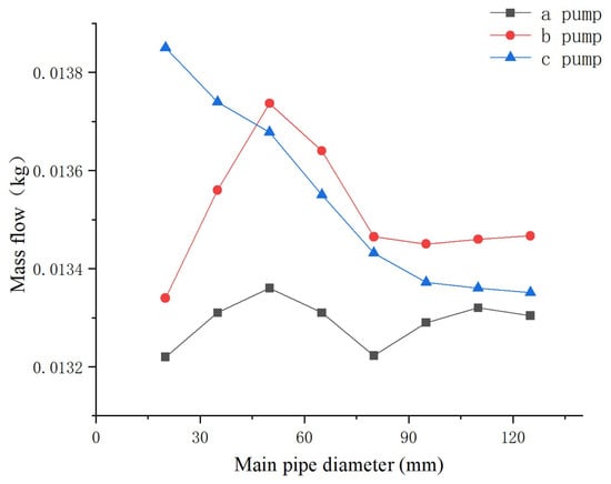
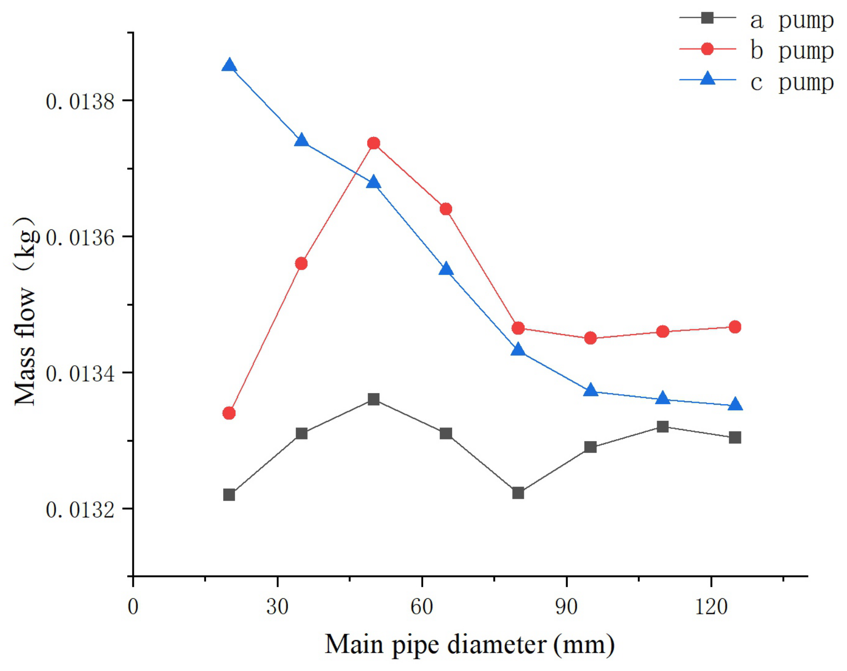
Figure 20 shows the evolution of the cumulative mass flow rate per unit time of each pump head with the manifold diameter. The cumulative mass flow rate of pump a exhibits a fluctuating trend of first increasing and then decreasing as the diameter increases, with only slight variations overall, remaining within the range of 0.0132–0.01336 kg. The cumulative mass flow rate of pump b increases rapidly at first with increasing diameter, reaches its peak at a diameter of 50 mm, and then gradually decreases and tends to stabilize, finally remaining within the range of approximately 0.01346–0.01347 kg. In contrast, the cumulative mass flow rate of pump c decreases continuously with increasing diameter, dropping gradually from about 0.01385 kg at 25 mm to about 0.01335 kg at 125 mm, showing an overall monotonically decreasing trend.
Figure 20.
Evolution of the cumulative mass flow rate per unit time of each pump head with manifold diameter.
From the comparison among the three pump heads, under small-diameter conditions, the cumulative mass flow rate of pump c is significantly higher than those of pumps a and b. As the diameter increases, the differences in cumulative mass flow rate among the three pump heads gradually decrease, and under large-diameter conditions, the values of the three pumps tend to become close to one another.
4. Limitations
Despite the insights provided by the present numerical study, several limitations should be acknowledged. First, the numerical model is based on a two-dimensional simplification of the triplex diaphragm hose pump. Although the two-dimensional model captures the dominant flow characteristics within the pump chambers and the manifold, it cannot fully reproduce the three-dimensional flow structures, such as secondary flows and spanwise variations, which may introduce quantitative deviations in the predicted flow-field parameters. Second, the deformation of the hose wall is prescribed in advance through a user-defined function based on a Gaussian distribution, rather than being determined by the actual fluid–structure interaction. This one-way coupling treatment neglects the feedback of the fluid pressure on the hose deformation, which may affect the accuracy of the predicted volumetric efficiency and pressure pulsation. Third, the gap model is adopted to treat the narrow gap between the ball valve and the valve seat during the opening and closing process. Although the gap model provides a reasonable approximation of the valve leakage, the actual leakage behavior is more complex, especially during the rapid valve-closing stage, and may deviate from the model predictions. Finally, the numerical results are validated only indirectly through grid independence analysis and comparisons with theoretical expectations, and no direct experimental validation of the flow-field parameters has been performed in this study. Therefore, the quantitative conclusions should be interpreted with caution. Future work will focus on three-dimensional modeling, fully coupled fluid–structure interaction simulations, and experimental measurements to further verify and refine the present results.
5. Conclusions
This study establishes a dynamic mesh-based FSI model of the triplex diaphragm hose pump and systematically investigates its internal flow-field characteristics as well as the effects of the operating flow rate and the inlet manifold diameter. The main conclusions are as follows:
- (1)
- A dynamic mesh-based FSI model balancing accuracy and efficiency is established: the hose deformation is driven by a UDF with a Gaussian distribution, and the ball valve motion is simulated by the gap model combined with the 6DOF solver, effectively reproducing the internal FSI process. The grid independence is verified by two indicators, the total mass flow rate and the peak chamber pressure, whose relative errors between the 330,000-cell and 371,000-cell meshes are only 0.05% and about 0.09%, respectively, ensuring both the computational accuracy and efficiency.
- (2)
- The flow field alternates with the suction and discharge strokes, with flow separation at the valve ports and a “double-peak–single-valley” outlet pulsation with backflow (the peak and valley mass flow rates of pump a are about 0.12 and 0.02 kg/s). Owing to the positional effects, the three pumps exhibit a “water-grabbing” flow distribution: within 1 s (two working cycles), the cumulative conveyed masses of pumps a, b, and c are 0.02258, 0.02299, and 0.02283 kg. The chamber pressure peaks at about 15 kPa, whereas the minimum pressure of pump c reaches about kPa, lower than those of pumps a and b (about kPa). High turbulent kinetic energy 0.1–0.5 concentrates at the valve ports, mainly induced by the valve opening and closing.
- (3)
- The flow rate increases linearly with the hose amplitude (the mean manifold velocity rises from 0.299 to 0.993 m/s as A increases from 0.006 to 0.020 m), enhancing the delivery capacity but intensifying the chamber-pressure pulsation, since the larger stroke displacement per cycle expands the pressure fluctuation range and aggravates the alternating load on the structure. The normalized pulsation rates and decrease from 0.3093 and 0.3637 at m to 0.1389 and 0.1823 at m, because the absolute pulsation amplitude grows only slightly relative to the mean flow level. The three pumps show different sensitivities owing to the positional effect, with pump a being the least sensitive and pump c the most sensitive.
- (4)
- A larger manifold diameter reduces the manifold velocity and weakens the positional effects, improving the flow distribution: the mean velocity decreases from 2.91 m/s at 25 mm to 0.66 m/s at 100 mm, and the pulsation rate decreases from 0.408 to 0.280, because the enlarged cross-section weakens the flow inertia and the local disturbances that cause the flow imbalance; the improvement tends to become marginal beyond about 100 mm, as the regulating effect of further enlarging the diameter saturates. The three pumps differ in sensitivity: pump a, closest to the inlet, is the most stable, while pump c, farthest from the inlet, is the most sensitive owing to the strongest accumulated flow-path loss and interference from the upstream pump heads.
Based on these findings, within the range of operating conditions investigated, a manifold diameter near 100 mm is suggested, while excessive enlargement is not recommended from the perspective of cost-effectiveness; the operating amplitude should be chosen by balancing the delivery requirement against the pressure pulsation and the structural fatigue; and, for parallel multi-pump systems, the flow-rate imbalance and the higher sensitivity of the pump head farthest from the inlet should be taken into account in the design and operation monitoring.
Author Contributions
Conceptualization, W.Y.; Methodology, H.C.; Software, Z.B.; Formal analysis, H.C. and S.Z.; Investigation, S.C. and H.X.; Resources, W.Y. and H.X.; Visualization, Y.L.; Writing—original draft, H.C.; Writing—review and editing, W.Z., Y.L., Z.B. and W.Y.; Supervision, W.Z.; Project administration, S.Z.; Funding acquisition, H.X. All authors have read and agreed to the published version of the manuscript.
Funding
This work was supported by the National Natural Science Foundation of China [grant no. 12572339]; the Natural Science Foundation of Zhejiang Province [grant no. LZ24A020005, LQN26A020008, ZCLQN25A0201]; and the Science and Technology Department of Zhejiang Province [grant no. 2024C01228].
Data Availability Statement
The original contributions presented in this study are included in the article. Further inquiries can be directed to the corresponding authors.
Conflicts of Interest
Author Shengyi Chen was employed by Tix Technology Group Lishui Fluid Equipment Co., Ltd. Author Hongxing Xu was employed by Zhongcheng Valve Group Co., Ltd. The remaining authors declare that the research was conducted in the absence of any commercial or financial relationships that could be construed as potential conflicts of interest.
References
- Ling, X. Reciprocating Piston Diaphragm Pump. Min. Process. Equip. 2002, 26–27+2–4+25. [Google Scholar]
- Vetter, G.; Yao, T. Safe and reliable diaphragm pump. Electromechanical. Equip. 1994, 6, 21–30+37. [Google Scholar]
- Pei, J. Application of pneumatic diaphragm pump in pharmaceutical and food production. Chem. Pharm. Eng. 2009, 30, 23–26. [Google Scholar]
- Dai, G.; Fan, W. Application of pneumatic diaphragm pump in coal mine underground drainage system. Mineral. Mag. 2014, 30, 110–111. [Google Scholar]
- Ling, X. Technical parameters and core technology of reciprocating piston diaphragm pump. Evelopment Innov. Mach. Electr. Prod. 2006, 19, 45–48. [Google Scholar]
- Ling, H. Fault Analysis and Operation Maintenance Installation on Feluwa Hose Diaphragm Piston Pumps. Large Scale Nitrogenous Fertil. Ind. 2022, 45, 391–393. [Google Scholar]
- Li, M. Application of GEHO Piston Diaphragm Pumps in Multi–Nozzle Coal Water Slurry Gasification Units. Nitrogenous Fertil. Syngas 2022, 50, 32–34. [Google Scholar]
- Watson-Marlow Fluid Technology Solutions Group. Study of Peristaltic Hose Pump Technology in Precious Metal Mining: More Efficient Operation and Higher Productivity Time; Watson-Marlow Fluid Technology Solutions: Falmouth, UK, 2020. [Google Scholar]
- Wang, K.; Gu, X.S.J. Application and commissioning of pneumatic diaphragm pumps in bilge water system of semisubmersible platforms. Mech. Electr. Eng. Technol. 2022, 51, 238–340. [Google Scholar]
- Pei, J.; He, C.; Lv, M.; Huang, X.; Shen, K.; Bi, K. The valve motion characteristics of a reciprocating pump. Mech. Syst. Signal Process. 2016, 66, 657–664. [Google Scholar] [CrossRef] [Scilit]
- Iannetti, A.; Stickland, M.T.; Dempster, W.M. An advanced CFD model to study the effect of non–condensable gas on cavitation in positive displacement pumps. Open Eng. 2015, 5, 323–331. [Google Scholar] [CrossRef] [Scilit]
- Li, W.; Mckeown, A.; Yu, Z. Correction of cavitation with thermodynamic effect for a diaphragm pump in organic Rankine cycle systems. Energy Rep. 2020, 6, 2956–2972. [Google Scholar] [CrossRef] [Scilit]
- Alberto, M.; Manuel, F.; Andrés, M. Numerical methodology for the CFD simulation of diaphragm volumetric pumps. Int. J. Mech. Sci. 2019, 150, 322–336. [Google Scholar] [CrossRef] [Scilit]
- Alberto, M.; Manuel, F. Unsteady three-dimensional modeling of the Fluid–Structure Interaction in the check valves of diaphragm volumetric pumps. J. Fluids Struct. 2019, 90, 432–439. [Google Scholar] [CrossRef] [Scilit]
- van Rijswick, R.; Talmon, A.; van Rhee, C. Fluid structure interaction (FSI) in piston diaphragm pumps. Can. J. Chem. Eng. 2016, 94, 1116–1126. [Google Scholar] [CrossRef] [Scilit]
- Shi, Y.; Yang, S. Investigation on dynamic characteristics of a plate–type discharge valve in a diaphragm pump for SCR system by two–way FSI model. Proc. Inst. Mech. Eng. Part D J. Automob. Eng. 2020, 234, 1197–1209. [Google Scholar] [CrossRef] [Scilit]
- Pan, X.; Yang, S. Investigation on the Dynamic Characteristics of Port Valves in a Diaphragm Pump for Exhaust Gas Treatment System by FSI Modeling. IEEE Access 2019, 7, 57238–57250. [Google Scholar] [CrossRef] [Scilit]
- Chen, H.; Ma, J. Fluid–Structure Interaction Modeling and Vibration Characteristics of Check Valves in High–Pressure Diaphragm Pumps. Mech. Sci. Technol. 2024, 43, 1199–1206. [Google Scholar]
- Gaudio, P.; Lupelli, I.; Malizia, A. Numerical modelling and performance optimization study of a diaphragm pump for drug infusion. In Proceedings of the 2012 COMSOL Conference; COMSOL, Inc.: Burlington, MA, USA, 2012. [Google Scholar]
- Zhang, H.; Shi, Y. Optimal Design of Disc–Shaped Rubber Diaphragms for Diaphragm Pumps. China Rubber Ind. 2017, 64, 174–178. [Google Scholar]
- Zhang, H.; Qiang, Z. Optimal Design of Piston Assembly for Hose Diaphragm Pump Based on ANSYS. Mach. Des. Manuf. Eng. 2022, 51, 33–37. [Google Scholar]
- Jia, B.; Zhao, Z.; Wang, X.; Chen, C.; Ma, X.; Wu, J.; Yang, L.; Politaeva, N. Local film thickness in relation to the droplet topological structure of droplet falling film on micro–nano structured horizontal tubes. Case Stud. Therm. Eng. 2026, 83, 108125. [Google Scholar] [CrossRef] [Scilit]
- Suo, S.; Li, M.; Jiang, L.; Dai, Y.; Ali Hamid, M.; Zhang, Y.; Qi, H.; Xie, M. Analysis of turbulent structural characteristics and dynamic heat transfer mechanisms in a packed structure wake rectifier using large eddy simulation method. Chem. Eng. Sci. 2026, 334, 124305. [Google Scholar] [CrossRef] [Scilit]
- Jia, B.; Huang, Z. Thermophysical, multiphase-flow, geochemical, and microbial controls on combined H2–CO2 storage in depleted gas reservoirs and saline aquifers. Fuel 2027, 429, 140747. [Google Scholar] [CrossRef] [Scilit]
- Ma, X.; Zhang, L.; Wang, W.; Yan, Y.; Du, C. The shell shape optimization and fluid–structure interaction simulation of hose pump in water-fertilizer integrated fertilizer application. Sci. Rep. 2022, 12, 3284. [Google Scholar] [CrossRef] [Scilit] [PubMed]

Disclaimer/Publisher’s Note: The statements, opinions and data contained in all publications are solely those of the individual author(s) and contributor(s) and not of MDPI and/or the editor(s). MDPI and/or the editor(s) disclaim responsibility for any injury to people or property resulting from any ideas, methods, instructions or products referred to in the content. |
© 2026 by the authors. Licensee MDPI, Basel, Switzerland. This article is an open access article distributed under the terms and conditions of the Creative Commons Attribution (CC BY) license.