Improving Harvesting Efficiency and Sustainability Through Lightweight Visual Perception: COS-DETR for Resource-Constrained Tea-Harvesting Robots

Abstract

Visual perception is a key challenge for tea-harvesting robots because tender buds must be distinguished from dense foliage under variable illumination and localized rapidly enough to support grasping on embedded hardware. We developed COS-DETR, a detector based on RT-DETR that incorporates a Faster CGLU block, the OmniKernel module with an internal Frequency–Spatial Attention Module (FSAM), and SPDConv. We also evaluated a compression pipeline that combines layer adaptive magnitude pruning (LAMP), channel pruning, and Mimic + Linear knowledge distillation. The uncompressed model achieved 87.1% $mA{P}_{0.5}$, the highest value among the evaluated detectors. After pruning and distillation, the model achieved 85.7% $mA{P}_{0.5}$ and 58.1 FPS on an NVIDIA Jetson Orin NX, with a 37.3% reduction in computational cost at the expense of only 1.4 percentage points of $mA{P}_{0.5}$. In 15 static field trials, the integration of this detector with a stereo camera and a Delta manipulator yielded absolute positioning errors below 5 mm. As the harvesting platform remains an experimental prototype, these trials validated static target positioning only; continuous dynamic picking was not performed, so the picking success rate and the missed-detection rate under dynamic conditions are not reported in this study. These results indicate that a compressed vision transformer detector can provide the speed, accuracy, and positional precision required for robotic process control in precision tea harvesting within the static positioning scope evaluated here.

1. Introduction

Premium tea is a high-value crop with a narrow three- to five-day harvesting window, during which only single buds or tender shoots should be collected. Manual plucking is labor-intensive and increasingly constrained by seasonal labor shortages, which can reduce production efficiency and product quality [1,2]. Robotic harvesting could alleviate these constraints by automating shoot detection and plucking [3,4,5]. However, field perception remains challenging because tender buds resemble mature leaves in color and shape and frequently occur in dense, cluttered backgrounds. The perception system must also provide bud coordinates rapidly enough to support grasp planning. High-accuracy detectors are computationally demanding, which complicates real-time deployment on low-power embedded hardware [6,7].

Beyond detector design, a tea-harvesting robot must integrate sensing, embedded computation, and actuation into one coordinated process. Data-driven distributed monitoring and plug-and-play (PnP) control frameworks rely on local measurements exchanged between subsystems for system-wide diagnosis and optimization, without a single central computing node [8]. Projection-based extensions further decompose measurements into disturbance-related and disturbance-free subspaces to support robust fault monitoring and distributed disturbance rejection in interconnected systems [9]. These control perspectives emphasize local computation on each subsystem. In the present study, the on-device perception module supplies tea bud positions to the localization and manipulator control modules, following the same principle of distributed local processing.

Studies of selective harvesting robots identify crop variability, occlusion, illumination, target accessibility, cycle time, and the coordination between perception and the end effector as persistent barriers to reliable field operation [10,11,12]. These barriers also apply to tea harvesting, where cultivar morphology, canopy structure, season, and management practice can shift the distribution of field images. The perception system must therefore remain robust when these factors vary, while still meeting the computational limits of the onboard platform.

Early machine vision studies demonstrated the value of image preprocessing and handcrafted feature selection for fine visual inspection [13,14]. Deep learning later enabled end-to-end feature learning with convolutional neural networks (CNNs), reducing the reliance on handcrafted features [15]. Earlier tea-vision studies used CNNs for tea recognition and classification. Zhang et al. [16] evaluated AlexNet and ResNet-50 for tea recognition. Yan et al. [17] combined MobileNetV2 with a multi-scale dense-sampling module to reduce computational cost. Zhang et al. [18] paired MobileNetV2 with multiclass TrAdaBoost for transfer learning. Yang et al. [19] combined semi-supervised learning with conventional image processing to identify tender leaves with limited labeled data. Wang et al. [20] used hyperspectral imaging and a multi-branch kernel attention network to assess tea leaf quality at different picking stages. These methods cover recognition and quality assessment, but robotic harvesting additionally requires the spatial location of each target bud. For lightweight agricultural object detection, Yang et al. [21] proposed CFD-DETR, an RT-DETR variant for tomato ripeness detection that incorporates CAEfficientViT and Wise-SIoU. Building on these advances, this study adopts RT-DETR as the baseline and examines directional feature extraction at multiple scales, joint frequency and spatial feature refinement, and spatial rearrangement for tea bud detection. Each modification is evaluated for its effect on detection accuracy and computational cost on the present dataset and embedded platform.

Although RT-DETR excels in object detection tasks, it still faces challenges in recognizing premium tea buds. The shapes and colors of premium tea vary significantly across growth stages, complicating recognition. Moreover, the model’s local receptive fields struggle to capture the fine grained textural differences necessary for accurate identification, resulting in insufficient generalization for tea recognition [22].

The specific objectives of this research are:

• To develop COS-DETR, a lightweight visual perception framework that addresses the dual challenges of fine tea bud recognition and real-time inference on embedded platforms, by integrating the Faster CGLU block, the OmniKernel module with its internal FSAM, and SPDConv into the RT-DETR architecture.
• To design a hybrid model compression pipeline that combines layer adaptive magnitude pruning (LAMP), channel pruning, and Mimic + Linear knowledge distillation, achieving a parameter reduction of ≥20% and a computational reduction of ≥35% while keeping $mA{P}_{0.5}$ above $85\%$.
• To evaluate the integration of the compressed detector, stereo positioning, and manipulator control through offline benchmarking and 15 static field positioning trials on an experimental prototype of a tea-harvesting platform built for this study, and to assess the feasibility and practical value of the detection, positioning, and grasping pipeline under the tested conditions. Because the platform is a research prototype rather than a production machine, this objective is limited to static positioning accuracy; continuous dynamic picking and the associated picking success rate and missed-detection rate are outside the scope of the present study.

2. Materials and Methods

2.1. Experimental Platform and Data Acquisition

2.1.1. Sample and Data Collection

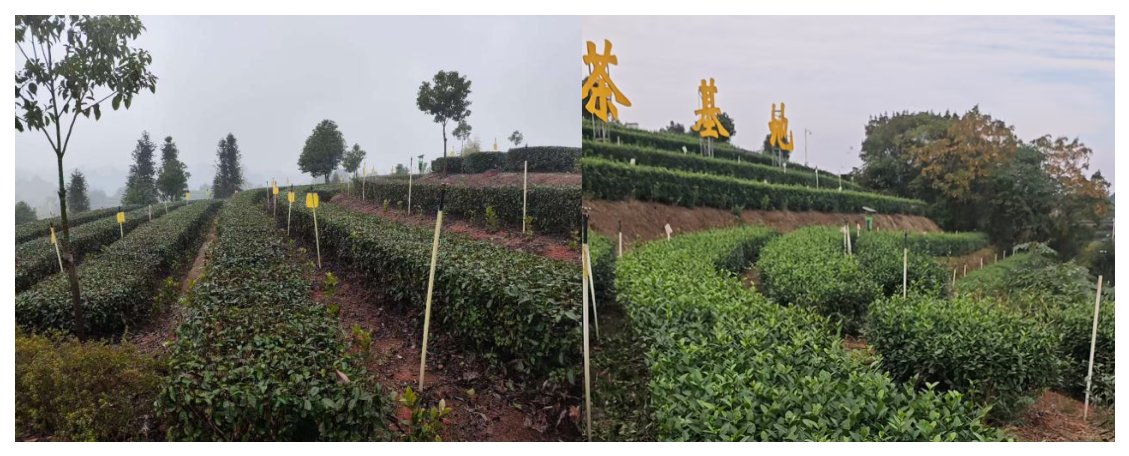
Data were collected in tea gardens of the Chuan Tea Group in Yibin City, Sichuan Province, China. The surveyed tea bushes were approximately 800 mm high and 1200 mm wide on average, with a spacing of about 450 mm. Maximum measured bush width reached 1480 mm in relatively flat areas, whereas bushes in steeper areas were narrower. These measurements describe the field geometry considered when configuring the experimental harvesting platform (Figure 1).

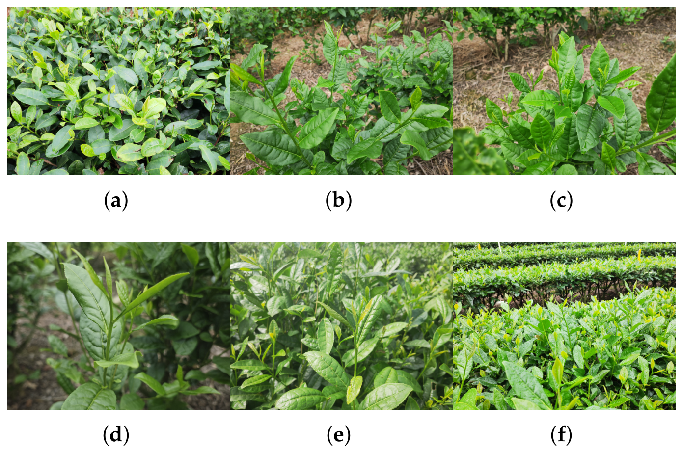
To account for the natural variation in leaf orientation and the illumination differences between weather conditions, images were collected from multiple viewpoints and under multiple lighting conditions: three viewpoints (overhead, left-oblique, and right-oblique), two lighting conditions (front lighting and backlighting), and one multi-plant scene setting. These six settings increase sample diversity and approximate the imaging conditions that the harvesting robot encounters in practice. The collected samples are shown in Figure 2.

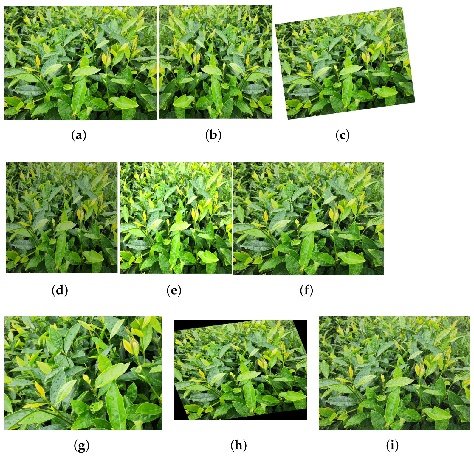
Following image acquisition, all samples were screened for image quality and target visibility. Images whose targets could not be annotated reliably were excluded, and the remaining annotations were checked manually for consistency. To increase visual diversity, the source images were augmented through brightness adjustment, image flipping, random rotation and cropping, Gaussian blurring, affine transformation, and noise injection, as illustrated in Figure 3.

The original images and their retained augmented versions yielded a total of 6240 images, comprising 1950 original images and 4290 retained augmented images. For partitioning, each original image and all of its retained augmented versions were treated as one source image group. The groups were randomly assigned to the training, test, and validation subsets in a 7:2:1 ratio, and no group was assigned to more than one subset. The training, test, and validation subsets each contained the original images and the retained augmented versions of their assigned groups.

The partition contained 1365 original training images, 390 original test images, and 195 original validation images. Included in the retained augmentations were the training, test, and validation subsets containing 4368, 1248, and 624 images, respectively.

2.1.2. Tea-Harvesting Robot Platform

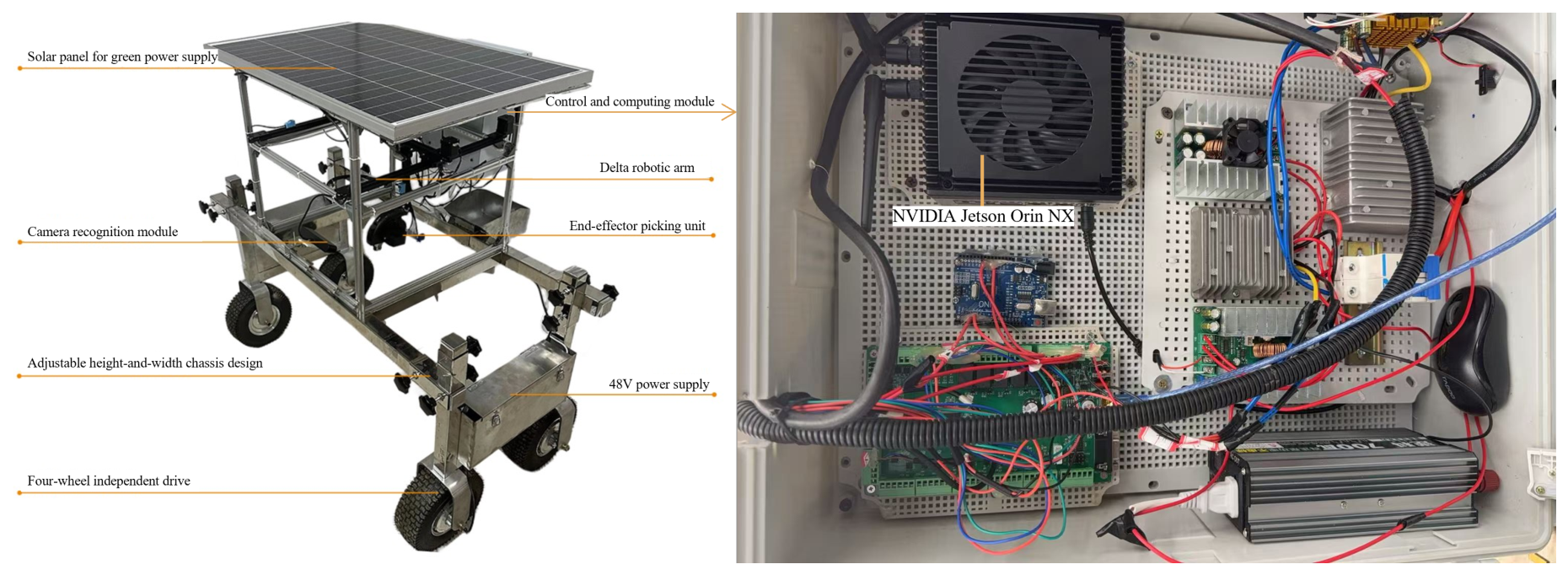
An experimental tea-harvesting platform was developed for the geographic and climatic conditions of the Chuan Tea Group plantation. The platform is an experimental prototype built for laboratory and limited field evaluation rather than a production harvesting machine. The platform consists of a visual perception module, a mechanical execution module, a control and computing module, a power supply module, and a mobile operation module (Figure 4). At its current stage of development, the platform supports detection, three-dimensional positioning, and single-target picking tests performed with the platform stationary; its perception, control, and actuation subsystems have not yet been integrated into a configuration capable of sustained continuous operation. This capability boundary defines the scope of the field validation reported in this study.

• Visual perception module: Intel RealSense D405 (Jabil Precision Industry Co., Ltd., Guangzhou, China) stereo depth camera and fixed adjustable lighting.
• Mechanical execution module: Delta robotic arm and an end effector.
• Control and computing module: NVIDIA Jetson Orin NX (NVIDIA Corporation, Santa Clara, CA, USA).
• Power supply module: 48 V lithium battery pack and solar panels.
• Mobile operation module: Mobile chassis with adjustable width and height.

2.1.3. Training Configuration and Parameter Settings

The experiments were conducted on a computer running Windows 10 with Python 3.8, PyTorch 2.7.1, and CUDA 12.0, equipped with an Intel Core i9-13900HX CPU and an NVIDIA GeForce RTX 4080 Laptop GPU with 12 GB of VRAM. All comparison experiments were conducted in the same computing environment. The training settings are listed in

Table 1. Training parameters.

Parameter	Value
Learning Rate	0.0001
Momentum	0.9
Weight Decay	0.0001
Optimizer	AdamW
Batch Size	4
Image Size	640 × 640
Number of Training Epochs	300

.

2.2. COS-DETR: Design and Implementation

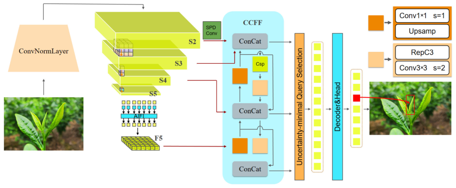
Figure 5 presents the COS-DETR architecture. COS-DETR extends RT-DETR with four modules that serve complementary functions. The Faster CGLU block [23] models nonlinear feature interactions through dynamic gating and strengthens robustness to cluttered backgrounds. The OmniKernel module captures texture patterns at different orientations and scales through its directional convolutional branches, while its internal FSAM branch [24] adds a frequency-domain context for global structure and spatial refinement for local detail. SPDConv [25] splits each feature map into spatial subregions and concatenates them along the channel axis, reducing resolution while preserving the sampled information at negligible additional cost. Together, these four additions sharpen the discrimination of bud texture and contour while keeping the computational cost manageable.

2.2.1. Input Feature Enhancement Module Based on BasicBlock Faster CGLU

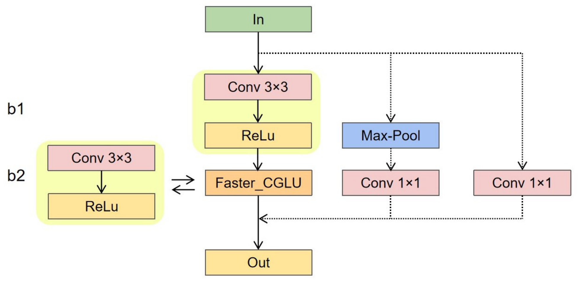
Input feature quality directly affects all subsequent feature modeling. Tea bud images combine rich texture, complex backgrounds, and highly variable object shapes, so feature extraction must handle these conditions at low computational cost. To improve feature learning in the residual block, the BasicBlock design replaces the original second convolutional branch with a Faster CGLU block (Figure 6).

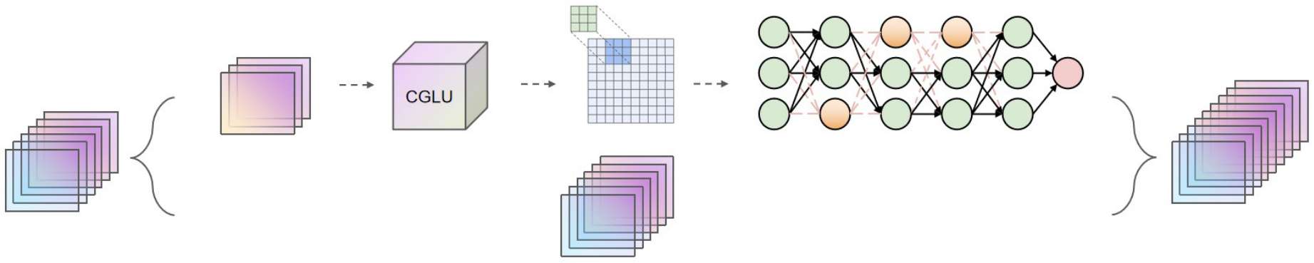
The two convolutional layers in a standard residual block perform only simple linear transformations. The Faster CGLU block combines a partial convolution with the CGLU gating mechanism so that global channel interactions and local spatial details are modeled in parallel. In this design the network learns channel importance weights, which increases the modeling capacity of the residual block at a modest cost. The block is illustrated in Figure 7.

A $3\times 3$ partial convolution is first applied to a subset of the input channels:

$$\begin{array}{c}\hfill \begin{array}{c}\hfill X_{\mathrm{partial}}=\mathrm{PartialConv}\left(X\right)\end{array}\end{array}$$

(1)

where $X_{\mathrm{partial}}\in {\mathbb{R}}^{N\times C_{\mathrm{partial}}\times H\times W}$ is the output after the partial convolution; $C_{\mathrm{partial}}={\displaystyle \frac{1}{n_{\mathrm{div}}}}·C_{\mathrm{in}}$, i.e., the proportion of channels in the partial branch, is controlled by the hyperparameter $n_{\mathrm{div}}$; the input feature is $X\in {\mathbb{R}}^{N\times C_{\mathrm{in}}\times H\times W}$. We then use CGLU to dynamically adjust the channel dimension, and finally recover the input features through a residual connection, as follows:

$$\begin{array}{c}\hfill \begin{array}{c}\hfill Y=X_{\mathrm{shortcut}}+\mathrm{DropPath}\left(\mathrm{CGLU}\left(X_{\mathrm{partial}}\right)\right)\end{array}\end{array}$$

(2)

where $X_{\mathrm{shortcut}}$ denotes the input shortcut (residual) branch that ensures the propagation of global information; DropPath is a regularization technique that randomly drops a subset of residual paths to enhance the network’s generalization capability.

CGLU splits the projected features into two branches. The main branch $X_1$ is used for further spatial feature extraction, and the gating branch $X_2$ computes dynamic weights that modulate feature importance. Given $X\in {\mathbb{R}}^{N\times C_{\mathrm{in}}\times H\times W}$, a $1\times 1$ convolution first projects the channel features, and the output is divided into the main feature map $X_1$ and the gating signal $X_2$. This process is formulated as follows:

$$\begin{array}{c}\hfill \begin{array}{c}\hfill X_1,X_2=\mathrm{Conv}1\times 1\left(X\right).\mathrm{chunk}\left(2,dim=1\right)\end{array}\end{array}$$

(3)

The main feature branch $X_1$ preserves the primary information of the input features and serves as the key component for subsequent spatial feature extraction. $X_1$ is passed to a depthwise convolution layer to capture local spatial relationships, while $X_2$ generates dynamic weights through a nonlinear activation function:

$$\begin{array}{c}\hfill \begin{array}{c}\hfill X_{\mathrm{gate}}=\sigma \left(X_2\right)\end{array}\end{array}$$

(4)

Then, through dynamic feature adjustment, adaptive weight modulation is achieved to selectively enhance or suppress the importance of features. The overall operation of CGLU can be summarized by the following equations:

$$\mathrm{CGLU}\left(X\right)=\mathrm{Conv}1\times 1\left(\mathrm{DWConv}\right.\left(\left.\mathrm{Conv}1\times 1\left(X\right)\left[:,:C_{\mathrm{hidden}}\right]\right)\right.\odot \left.\sigma \left(\mathrm{Conv}1\times 1\left(X\right)\left[:,C_{\mathrm{hidden}}:\right]\right)\right)$$

(5)

Here, $C_{\mathrm{hidden}}={\displaystyle \frac{2}{3}}·C_{\mathrm{in}}$ denotes the hidden-channel dimension. We refer to the combination of partial convolution and CGLU as Faster CGLU, and to the modified residual block as a BasicBlock with Faster CGLU.

2.2.2. Feature Extraction Based on OmniKernel and SPDConv

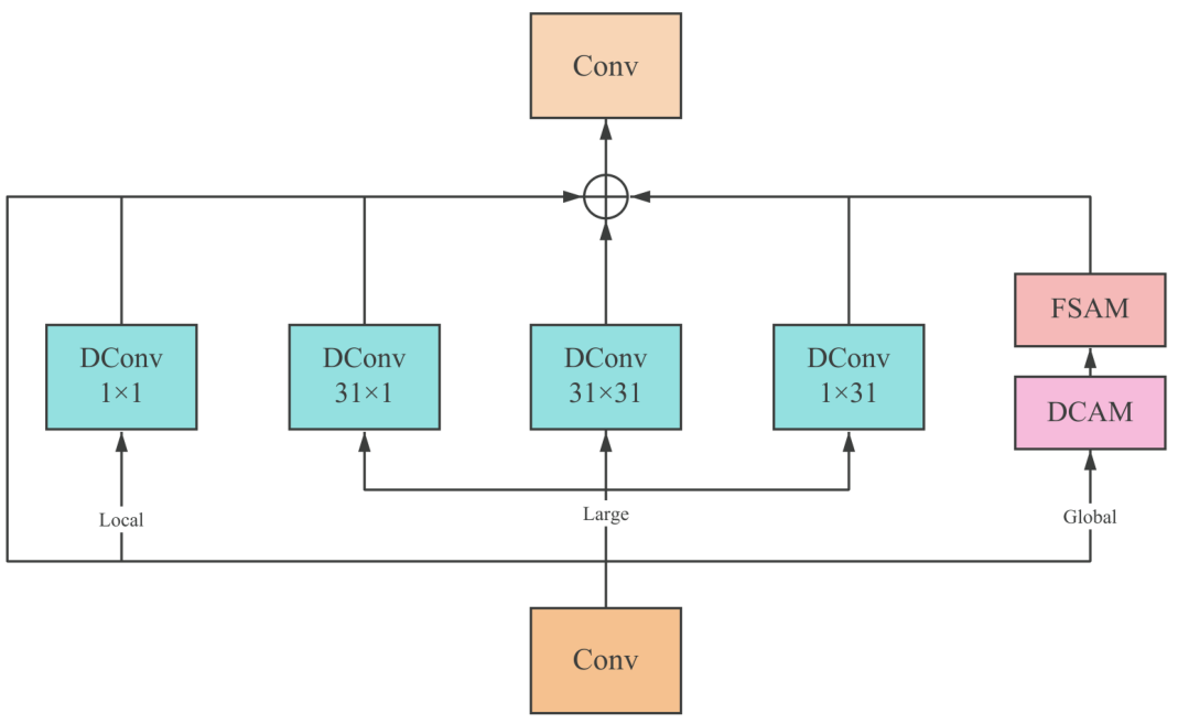
To improve the modeling of complex tea bud textures, this study integrates the OmniKernel module (Figure 8).

OmniKernel applies parallel convolutional branches with kernel sizes of $31\times 31$, $31\times 1$, $1\times 31$, and $1\times 1$, together with a $3\times 3$ depthwise convolution branch. The $31\times 1$ and $1\times 31$ branches capture directional context, the $31\times 31$ branch captures broader spatial structure, the $1\times 1$ branch models channel interactions, and the $3\times 3$ branch captures local details. The branch outputs, together with the frequency and spatial attention output $X_{FS}$ described below, are summed element-wise with the residual input:

$$\begin{array}{c}\hfill \begin{array}{c}\hfill X_{\mathrm{Omni}}=X+X_{31\times 1}+X_{1\times 31}+X_{31\times 31}+X_{1\times 1}+X_{FS}\end{array}\end{array}$$

(6)

The residual connection preserves the original input and facilitates gradient propagation. By combining directional, multiscale, and local feature extraction, OmniKernel improves the representation of tea buds whose textures are complex and whose scales vary widely.

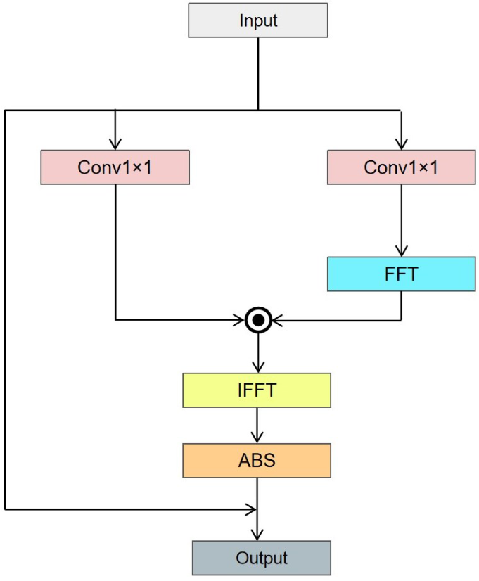
To balance global context and local texture, the Frequency–Spatial Attention Module (FSAM) is integrated into OmniKernel (Figure 9). FSAM combines context from the frequency domain with details from the spatial domain. In this study, FSAM was first evaluated as part of the complete OmniKernel stage, and its contribution was then examined separately using a control model in which the FSAM branch was disabled while the rest of COS-DETR was retained.

To derive the frequency domain representation from the input feature map $X\in {\mathbb{R}}^{C\times H\times W}$, we apply the Fast Fourier Transform (FFT) as follows:

$$\begin{array}{c}\hfill \begin{array}{c}\hfill X_{\mathrm{FFT}}=\mathrm{FFT}\left(X,\mathrm{norm}=‘\mathrm{backward}’\right)\end{array}\end{array}$$

(7)

Here, FFT denotes the two-dimensional fast Fourier transform, and $\mathtt{norm}\mathtt{=}\mathtt{‘}\mathtt{backward}\mathtt{’}$ specifies the normalization convention. To further enhance the discriminative ability of features, a frequency-channel attention mechanism (FCA) is introduced. Within the FCA module, the input features undergo Global Average Pooling to compress spatial dimensions into channel-wise statistics:

$$\begin{array}{c}\hfill \begin{array}{c}\hfill W_{\mathrm{FCA}}={\mathrm{Conv}}_{1\times 1}\left(\mathrm{GAP}\left(X\right)\right)\end{array}\end{array}$$

(8)

Here, GAP denotes global average pooling, and $W_{\mathrm{FCA}}\in {\mathbb{R}}^{C\times 1\times 1}$ denotes the frequency-channel attention weights. These weights are applied to $X_{\mathrm{FFT}}$ as follows:

$$\begin{array}{c}\hfill \begin{array}{c}\hfill X_{\mathrm{FCA}}=X_{\mathrm{FFT}}·W_{\mathrm{FCA}}\end{array}\end{array}$$

(9)

After frequency-channel weighting, the inverse fast Fourier transform (IFFT) maps $X_{\mathrm{FCA}}$ back to the spatial domain:

$$\begin{array}{c}\hfill \begin{array}{c}\hfill X_{\mathrm{IFFT}}=\mathrm{IFFT}\left(X_{\mathrm{FCA}},dim=\left(-2,-1\right)\right.\left.\mathrm{norm}=‘\mathrm{backward}’\right)\end{array}\end{array}$$

(10)

A spatial channel attention mechanism (SCA) is then applied to refine the spatial-domain features [26]. SCA summarizes $X_{\mathrm{IFFT}}$ through global average pooling and generates the channel weights $W_{\mathrm{SCA}}$ using a $1\times 1$ convolution:

$$\begin{array}{c}\hfill \begin{array}{c}\hfill W_{\mathrm{SCA}}={\mathrm{Conv}}_{1\times 1}\left(\mathrm{GAP}\left(X_{\mathrm{IFFT}}\right)\right)\end{array}\end{array}$$

(11)

Here, $W_{\mathrm{SCA}}\in {\mathbb{R}}^{C\times 1\times 1}$ denotes the spatial-channel attention weights obtained from the pooled spatial-domain features. These weights are broadcast over the spatial dimensions and applied element-wise:

$$\begin{array}{c}\hfill \begin{array}{c}\hfill X_{\mathrm{SCA}}=X_{\mathrm{IFFT}}\odot W_{\mathrm{SCA}},\end{array}\end{array}$$

(12)

where ⊙ denotes element-wise multiplication.

Finally, the spatially enhanced features $X_{\mathrm{SCA}}$ are fused with the residual input X:

$$\begin{array}{c}\hfill \begin{array}{c}\hfill X_{\mathrm{out}}=\alpha ·X_{\mathrm{SCA}}+\beta ·X\end{array}\end{array}$$

(13)

Here, $\alpha$ and $\beta$ are learnable parameters that balance the enhanced and residual branches.

SPDConv combines a space-to-depth rearrangement with a subsequent stride-1 convolutional block [25]. With the batch dimension omitted for simplicity, let $X\in {\mathbb{R}}^{C\times H\times W}$, where C, H, and W denote the channel count, height, and width, respectively. For even H and W, the input is divided into four interleaved spatial subsets using zero-based indexing:

$$\begin{array}{c}\hfill \begin{array}{c}\hfill \begin{array}{cc}\hfill X_1& =X[:,0:H:2,0:W:2],\hfill \\ \hfill X_2& =X[:,1:H:2,0:W:2],\hfill \\ \hfill X_3& =X[:,0:H:2,1:W:2],\hfill \\ \hfill X_4& =X[:,1:H:2,1:W:2].\hfill \end{array}\end{array}\end{array}$$

(14)

The notation $a:b:2$ selects every second element from index a up to, but excluding, b. The four subsets correspond to the top-left, bottom-left, top-right, and bottom-right positions within each $2\times 2$ spatial block. Each subset has dimensions $C\times (H/2)\times (W/2)$.

The subsets are concatenated along the channel dimension:

$$\begin{array}{c}\hfill \begin{array}{c}\hfill X_{\mathrm{split}}={\mathrm{Concat}}_{\mathrm{channel}}\left(X_1,X_2,X_3,X_4\right).\end{array}\end{array}$$

(15)

Thus, $X_{\mathrm{split}}\in {\mathbb{R}}^{4C\times (H/2)\times (W/2)}$. The space-to-depth step rearranges all input elements without discarding them and introduces no trainable parameters. A subsequent $3\times 3$ convolutional block with stride 1 fuses the rearranged features and produces the required output channels.

2.3. Lightweight Deployment Pipeline

Tea-harvesting robots run their perception models on embedded platforms with limited computing power and storage, so large detector networks often cannot meet real-time requirements. This study therefore combines layer adaptive magnitude pruning (LAMP) with channel pruning and the Mimic + Linear distillation strategy to obtain a compact model. Pruning removes redundant components of the network to reduce its computational workload, and distillation transfers knowledge from the original model to the compressed one. Together, these steps reduce the number of parameters and the computational complexity while keeping accuracy high, which meets the real-time and efficiency requirements of tea-harvesting robots.

2.3.1. LAMP with Channel Pruning

The core idea of LAMP is to dynamically adjust the pruning ratio based on the magnitude of the neurons in each layer, allowing for dynamic pruning that targets the characteristics of different layers. This approach helps to avoid redundant computations and maximally preserve the key structures of the network [27].

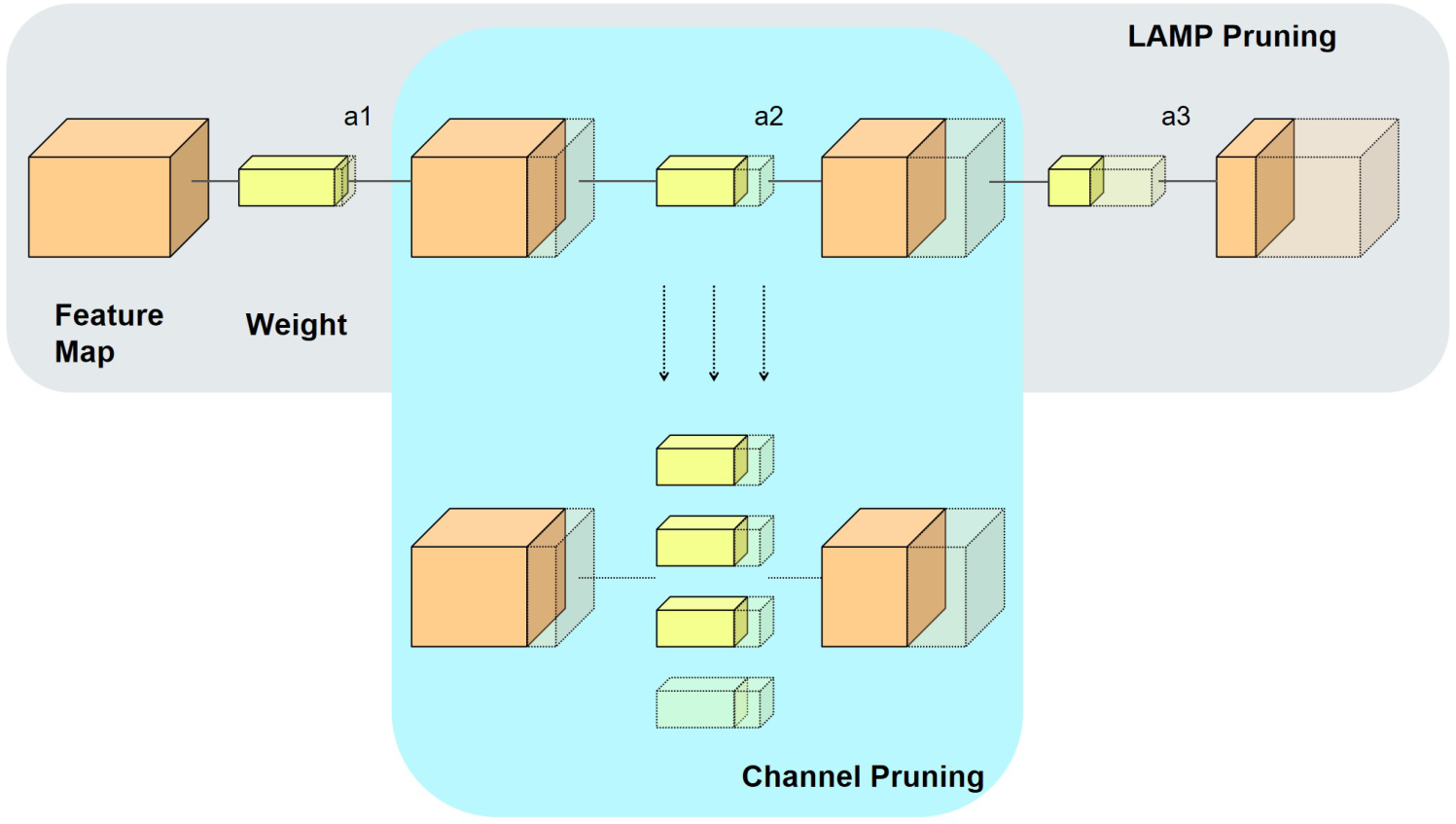
Although LAMP reduces the number of parameters, it does not directly reduce computational complexity. In convolutional networks, the computational cost is directly related to the number of channels in the convolutional layers [28]. Channel pruning therefore removes unimportant convolutional channels, rather than individual weights, which reduces both computation and memory. Performing LAMP first and channel pruning second allows the model to be optimized in two successive stages: LAMP removes redundant weights, and channel pruning removes redundant channels. The combined pipeline reduces computational cost and memory usage while adapting to the network structure, as shown in Figure 10.

Let the weight matrix of the l-th layer of the neural network be denoted as ${\mathrm{W}}^{\mathrm{l}}$, where ${\mathrm{W}}^{\mathrm{l}}\in {\mathbb{R}}^{C_{\mathrm{out}}\times C_{\mathrm{in}}\times K_{\mathrm{h}}\times K_{\mathrm{w}}}$. In this context, $C_{\mathrm{out}}$ and $C_{\mathrm{in}}$ signify the quantity of output and input channels, while $K_{\mathrm{h}}$ and $K_{\mathrm{w}}$ specify the spatial dimensions (height and width) of the convolutional kernel. For single weight pruning, traditional MP methods use L1 or L2 norms to measure the importance of weights. Specifically, $p=1$ corresponds to L1 pruning, while $p=2$ corresponds to L2 pruning. The MP method removes weights below a global pruning threshold determined by the global magnitude ranking of the weights. However, this approach overlooks the characteristics of different layers, which may lead to certain layers being overly pruned while others retain a significant amount of redundant parameters. The LAMP method improves upon this by introducing an inter-layer normalization factor ${\alpha }^l$ to optimize the pruning decision, i.e.,

$$\begin{array}{c}\hfill \begin{array}{c}\hfill M^l=\left|\right|W^l{\left|\right|}_p={\left({\sum }_{i,j,k,h}{\left|W_{i,j,k,h}^l\right|}^p\right)}^{{\displaystyle \frac{1}{p}}}\end{array}\end{array}$$

(16)

Given the weight matrix ${\mathrm{W}}^{\mathrm{l}}$ of a certain layer in the neural network, where each weight ${\mathrm{w}}_{\mathrm{i},\mathrm{j},\mathrm{k},\mathrm{h}}^{\mathrm{l}}$ represents the weight of the convolutional kernel between output channel $\mathrm{i}$ and input channel $\mathrm{j}$ at position $(k,h)$, its magnitude is defined as:

$$\begin{array}{c}\hfill \begin{array}{c}\hfill \left|W^l\right|=\{\left|w_{i,j,k,h}^l\right|\}\forall i,j,k,h\end{array}\end{array}$$

(17)

Calculate the sum of the magnitudes of the weights for each layer:

$$\begin{array}{c}\hfill \begin{array}{c}\hfill S^l=\sum _{i,j,k,h}\left|W_{i,j,k,h}^l\right|\end{array}\end{array}$$

(18)

Normalize the magnitudes of the weights across all layers to obtain the normalization factor ${\alpha }^l$:

$$\begin{array}{c}\hfill \begin{array}{c}\hfill {\alpha }^l={\displaystyle \frac{S^l}{{\sum }_k{S}^k}}\end{array}\end{array}$$

(19)

The normalization factor ${\alpha }^l$ adjusts the pruning rate of each layer according to its importance. LAMP uses this factor to compute the layer adaptive pruning threshold $T_p^l$, where p is the specified pruning rate and $\mathrm{percentile}(W,p)$ is the pth percentile of the weight magnitudes in that layer:

$$\begin{array}{c}\hfill \begin{array}{c}\hfill T_p^l={\alpha }^l·percentile\left(W,p\right)\end{array}\end{array}$$

(20)

After LAMP is completed, the network may still contain a significant number of redundant channels. Channel pruning further reduces computational load and storage requirements. The main process is as follows:

For the convolutional layer $\mathrm{l}$, which contains multiple channels ${\mathrm{C}}^{\mathrm{l}}=[\mathrm{C}{1}^{\mathrm{l}},\mathrm{C}{2}^{\mathrm{l}},\dots ,{\mathrm{CN}}^{\mathrm{l}}]$, the importance of each channel ${\mathrm{C}}_{\mathrm{i}}^{\mathrm{l}}$ is calculated by accumulating the magnitudes of all associated weights:

$$\begin{array}{c}\hfill \begin{array}{c}\hfill P_i={\displaystyle \frac{{\sum }_{j\in L_i}\mathrm{Magnitude}(i,j)}{{\sum }_{j\in L_i}\mathrm{Magnitude}(i,j)+\lambda }}\end{array}\end{array}$$

(21)

Here, $\mathrm{Magnitude}(i,j)$ is the sum of the weight magnitudes associated with channel i, and $\lambda$ is a balancing factor that keeps the importance scores away from extreme values. The scores $P_i$ rank the channels for pruning.

For all channel scores $P_i$, a pruning threshold $T_c$ is computed from the set $P=\{P_1,P_2,\dots ,P_N\}$ of all channel scores:

$$\begin{array}{c}\hfill \begin{array}{c}\hfill T_c=percentile\left(P,p\right)\end{array}\end{array}$$

(22)

2.3.2. Mimic + Linear Knowledge Distillation

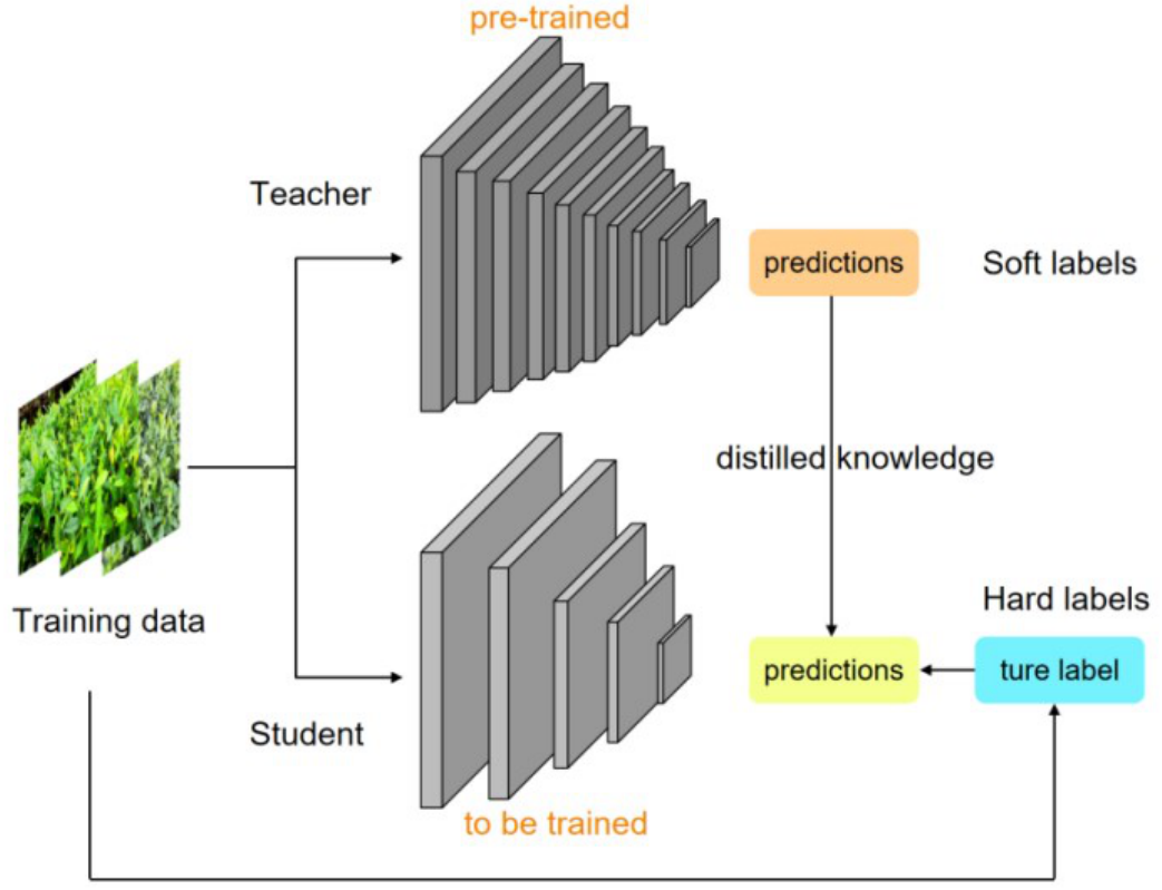
Pruning inevitably sacrifices accuracy for compactness [29]. Knowledge distillation recovers part of this loss by training a compact student network to match a high-performing teacher [30]. Figure 11 shows the approach adopted here. A Mimic loss aligns intermediate feature maps between the two networks, and a linearly decaying weight on the distillation loss gradually reduces the influence of the teacher as training progresses.

The distillation framework combines a logit loss and a feature loss. The logit component minimizes the gap between the output probability distributions of the two networks. The teacher and the student each produce a probability distribution through the Softmax function, and the gap between the two distributions is measured by the KL divergence, given by:

$$\begin{array}{c}\hfill \begin{array}{c}\hfill L_{log}=KL\left(p_t\Vert p_s\right)=\sum _i{p}_t\left(i\right)log{\displaystyle \frac{p_t\left(i\right)}{p_s\left(i\right)}}\end{array}\end{array}$$

(23)

Here, $p_t\left(i\right)$ and $p_s\left(i\right)$ are the predicted probabilities of the teacher and student models, respectively. Minimizing this divergence transfers the classification behavior of the teacher to the student.

A temperature parameter T is introduced to soften the teacher’s output distribution, which makes the imitation easier for the student. With temperature scaling, the distributions become

$$\begin{array}{c}\hfill \begin{array}{c}\hfill p_t={\displaystyle \frac{\exp (z_t/T)}{{\sum }_j\exp (z_{t,j}/T)}},p_s={\displaystyle \frac{\exp (z_s/T)}{{\sum }_j\exp (z_{s,j}/T)}}\end{array}\end{array}$$

(24)

where $z_t$ and $z_s$ are the unnormalized outputs of the teacher and student models, respectively, and a larger T produces a softer distribution. Minimizing the KL divergence between the scaled distributions encourages the student to learn the relative similarities between classes as represented by the teacher.

Let $f_t^{\left(i\right)}$ and $f_s^{\left(i\right)}$ denote the feature representations of the teacher and the student at the i-th layer. The mean squared error (MSE) between these representations defines the distillation loss of that layer:

$$\begin{array}{c}\hfill \begin{array}{c}\hfill L_{fea}^{\left(i\right)}={\Vert f_s^{\left(i\right)}-f_t^{\left(i\right)}\Vert }_2^2\end{array}\end{array}$$

(25)

where ${\Vert ·\Vert }_2^2$ denotes the squared Euclidean distance. Minimizing this loss aligns the intermediate features of the student with those of the teacher.

In multi-layer feature distillation [31], the losses of different layers contribute unevenly to the task, and the student may overfit to low-level features. Each layer loss is therefore weighted according to the importance of that layer, giving the weighted feature distillation loss:

$$\begin{array}{c}\hfill \begin{array}{c}\hfill L_{fea}={\displaystyle \sum _{i=1}^N}{\alpha }_i·L_{fea}^{\left(i\right)}={\displaystyle \sum _{i=1}^N}{\alpha }_i·{\Vert f_s^{\left(i\right)}-f_t^{\left(i\right)}\Vert }_2^2\end{array}\end{array}$$

(26)

Here, ${\alpha }_i$ is the weight of the i-th feature layer and N is the number of distilled layers. This weighting lets training focus on the layers that matter most for the final task: features closer to the output carry more semantic information and can receive higher weights, whereas low-level detail features can receive lower weights.

The linear decay strategy reduces the contribution of the distillation loss as training progresses, so that the student gradually relies less on the teacher and learns more from the task loss itself. Early in training, when the student has learned little, the teacher’s guidance is most useful and the distillation weight should be large. As training converges, this weight decreases, and the student relies increasingly on its own features and learned patterns.

A linear decay factor $D\left(t\right)$ controls the contribution of the feature distillation loss during training. Let E denote the total number of training epochs and t the current epoch index. The decay factor is defined as

$$\begin{array}{c}\hfill \begin{array}{c}\hfill D\left(t\right)=1-{\displaystyle \frac{t}{E}}.\end{array}\end{array}$$

(27)

The symbol T is reserved for the temperature parameter used in the softened probability distributions.

The distillation loss is multiplied by $D\left(t\right)$ before being added to the total loss:

$$\begin{array}{c}\hfill \begin{array}{c}\hfill L_{fea}^{adjusted}=D\left(t\right)·L_{fea}\end{array}\end{array}$$

(28)

2.4. Evaluation Metrics

The model performance is evaluated with four metrics: precision (P), frames per second (FPS), mean average precision (mAP), and giga floating-point operations (GFLOPs). The formulations of P, FPS, and mAP are given in Equations (29)–(31). Precision is the ratio of true positives (TPs) to all predicted positives and reflects the reliability of the detections; a higher value indicates fewer false positives. FPS measures the inference speed and indicates whether the model can process frames in real time. mAP is the average precision over the evaluated classes; $mA{P}_{0.5}$ reports the value at an IoU threshold of 0.5, and $mA{P}_{0.5:0.95}$ averages the values over IoU thresholds from 0.5 to 0.95. GFLOPs measures the computational cost of one forward pass and serves as an indicator of deployment feasibility.

$$\begin{array}{c}\hfill \begin{array}{c}\hfill \mathrm{P}={\displaystyle \frac{TP}{TP+FP}}\end{array}\end{array}$$

(29)

$$\begin{array}{c}\hfill \begin{array}{c}\hfill \mathrm{FPS}={\displaystyle \frac{N}{\mathrm{Total}\mathrm{time}}}\end{array}\end{array}$$

(30)

$$\begin{array}{c}\hfill \begin{array}{c}\hfill \mathrm{mAP}={\displaystyle \frac{1}{C}}{\displaystyle \sum _{c=1}^C}{\mathrm{AP}}_c\end{array}\end{array}$$

(31)

3. Results

3.1. Ablation Study

To validate the effectiveness of the proposed enhancement modules, five experiment groups were designed to quantify the contribution of each enhancement module and of the FSAM branch inside OmniKernel. The groups compare the baseline model with variants that successively add the Faster CGLU block, the OmniKernel module, and the SPDConv module, together with a variant in which the internal FSAM branch of the complete model is disabled. The changes in the metrics show the effect of each module on detection performance and any synergy among the modules.

Group 1 is the unmodified baseline and serves as the reference. Group 2 adds the Faster CGLU block to the feature extraction layer to verify the benefit of optimizing feature extraction. Group 3 further adds the OmniKernel module, whose convolutional kernels at several scales capture multiscale information of the targets. Group 4 additionally adds the SPDConv module, which restructures the spatial dimensions of the feature maps during downsampling to preserve detail. Group 5 retains the complete architecture of Group 4 but disables the internal FSAM branch of OmniKernel, so that the contribution of this branch can be examined separately from the cumulative additions. The experimental results are shown in

Table 2. Ablation study results.

Group	Add CGLU	Add OmniKernel	Add SPDConv	w/o FSAM	${\mathit{mAP}}_{0.5}$
1	×	×	×	–	0.846
2	✓	×	×	–	0.859
3	✓	✓	×	–	0.868
4	✓	✓	✓	×	0.871
5	✓	✓	✓	✓	0.866

In the Add CGLU, Add OmniKernel, and Add SPDConv columns, ✓ indicates that the module is added, whereas × indicates that it is not added. In the w/o FSAM column, ✓ indicates that the internal FSAM branch is disabled, whereas × indicates that it is retained. A dash (–) indicates that no separate comparison involving FSAM removal is performed for that group.

:

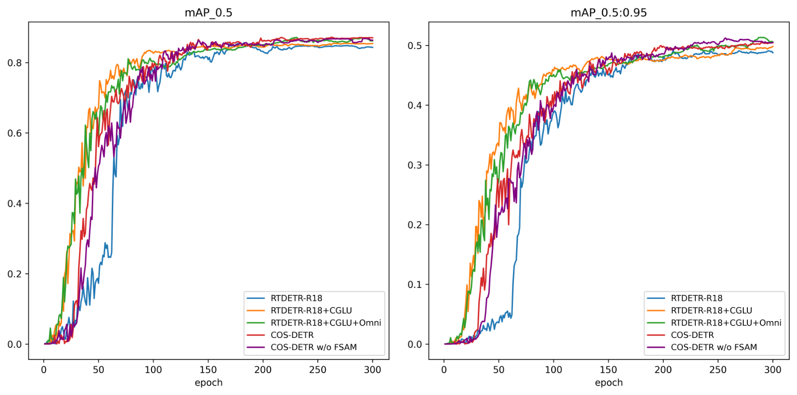
The baseline RT-DETR-R18 achieved an $mA{P}_{0.5}$ of 0.846, which shows that the base feature extraction network already provides a reasonable level of detection. In Group 2, adding the Faster CGLU block raised $mA{P}_{0.5}$ to 0.859, a gain of 1.3 percentage points over the baseline. In Group 3, adding the OmniKernel module on top of Group 2 raised $mA{P}_{0.5}$ to 0.868. Group 4 additionally incorporated the SPDConv module, which raised $mA{P}_{0.5}$ by a further 0.3 percentage points over Group 3. Group 5 retains the complete architecture of Group 4 but disables the internal FSAM branch of OmniKernel, which lowers $mA{P}_{0.5}$ to 0.866, a decrease of 0.5 percentage points relative to Group 4. This result indicates that the internal FSAM branch makes a positive but limited contribution to $mA{P}_{0.5}$ within the complete COS-DETR model on the present dataset; because the control is obtained by disabling this branch inside the complete model, it quantifies the marginal contribution of FSAM within the full architecture rather than the behaviour of this branch in isolation. The ablation results are illustrated in Figure 12.

3.2. Comparative Experiment

Table 3. Comparative experiment results.

Model	Precision (%)	Recall (%)	${\mathit{mAP}}_{0.5}$ (%)	${\mathit{mAP}}_{0.5:0.95}$ (%)
YOLOv8s	77.92	62.84	70.29	54.71
YOLO11s	74.09	62.16	71.41	54.07
YOLO12s	68.32	65.54	70.73	54.23
YOLOv5	81.5	78.0	78.1	41.3
YOLOv8	83.6	80.7	81.2	44.5
YOLOv11	82.3	79.8	78.3	42.9
RT-DETR-R18	82.7	84.2	84.6	47.8
RT-DETR-R50	83.7	84.7	85.4	48.2
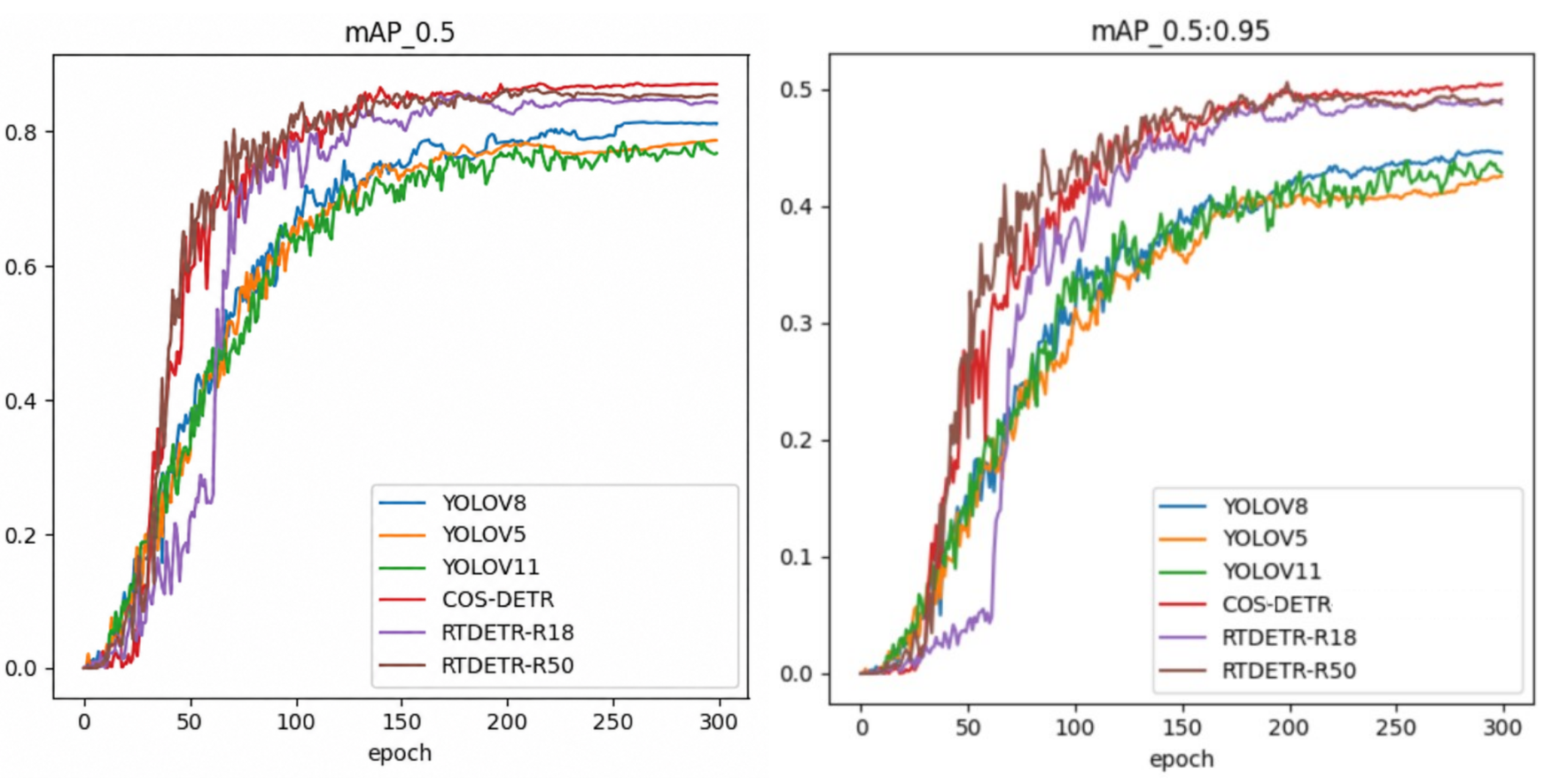
COS-DETR	85.6	85.0	87.1	50.4

and Figure 13 compares COS-DETR with the original YOLO and RT-DETR reference implementations and three additional small-scale configurations, YOLOv8s, YOLO11s, and YOLO12s. RT-DETR-R18 serves as the architectural baseline, while RT-DETR-R50 provides a deeper-backbone reference. The additional s-scale configurations extend the comparison to explicitly identified small models from multiple YOLO families. All results were obtained on the same independent test set using identical test images, annotations, and evaluation settings. The reported metrics are bounding-box precision, recall, $mA{P}_{0.5}$, and $mA{P}_{0.5:0.95}$.

On the test subset defined by the source image grouping, COS-DETR achieved the highest precision, recall, and $mA{P}_{0.5}$ among the evaluated implementations. Its $mA{P}_{0.5:0.95}$ of 50.4% was lower than those of the three small-scale configurations (YOLOv8s, YOLO11s, and YOLO12s) but exceeded those of the standard YOLO and RT-DETR models (Table 3).

3.3. Comparison of Different Network Models Under Challenging Field Conditions

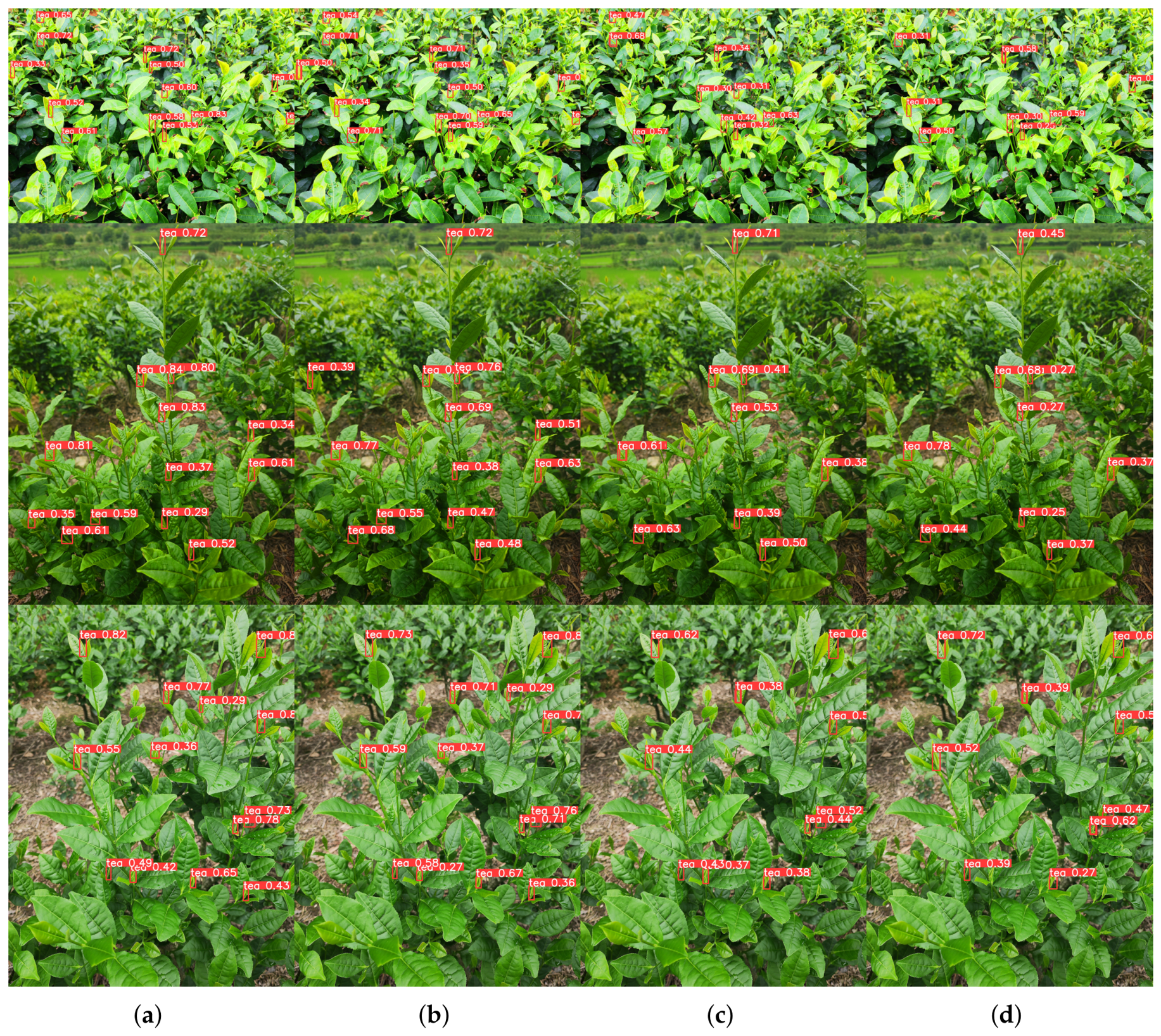
We tested YOLOv5, YOLOv8, RT-DETR-R18, and COS-DETR on images captured under uneven lighting, large viewing-angle variations, and cluttered backgrounds. Three representative scenes are shown in Figure 14. YOLOv5 missed the most targets: in the first scene, with strong backlighting, it detected only 8 of the visible buds (53%). YOLOv8 detected more targets but still missed several buds. RT-DETR-R18 remained stable as the lighting and viewpoint changed, and its detection rate across the three scenes exceeded that of YOLOv8, although its precision remained lower.

COS-DETR, which extends the RT-DETR backbone with multiscale feature aggregation and joint frequency and spatial attention, achieved the highest detection rate under the same harsh conditions. It identified 13 buds in the first scene (86%) and missed fewer buds than the other three models across all test images. On this challenging subset, COS-DETR reached an $mA{P}_{0.5}$ of 83% (

Table 4. Detection results on challenging field scenes.

Module	${\mathit{mAP}}_{0.5}$ (%)
YOLOv5	65.0
YOLOv8	67.0
RT-DETR-R18	78.0
COS-DETR	83.0

), which is 16 percentage points above YOLOv8 and 5 percentage points above RT-DETR-R18. These detection rates were obtained from single frames captured at fixed viewpoints and describe detection performance on individual images; they are distinct from the missed-detection rate of a continuous dynamic picking process, which was not measured in this study.

A quantitative analysis of the recognition images in Figure 14 was conducted, and the average results are shown in Table 4.

3.4. Pruning and Distillation Experiments

Pruning methods are compared in terms of accuracy, complexity, and speed. Accuracy is measured with $mA{P}_{0.5}$, complexity with GFLOPs and the number of parameters, and speed with FPS and average inference time. The results are shown in

Table 5. Experimental Results of Different Pruning Methods.

Pruning	Pruning Ratio	${\mathit{mAP}}_{0.5}$ (%)	GFLOPs	Parameters	FPS	Average Latency
None	None	87.1	54.4	16,019,172	49.6	12.96
LAMP + Cl	1.3	85.5	38.9	13,166,188	55.8	10.13
LAMP + Cl	1.5	84.2	35.3	12,892,196	58.1	9.50
LAMP + Cl	1.7	84.0	34.1	12,768,324	59.4	8.26
LAMP	1.3	86.1	41.5	14,077,252	43.3	15.13
LAMP	1.5	85.1	36.2	13,163,548	51.9	12.27
LAMP	1.7	84.6	35.5	12,930,188	54.3	11.01
L1	1.3	86.3	41.4	14,261,764	43.1	15.25
L1	1.5	83.8	35.6	12,959,028	43.7	14.98
L1	1.7	81.8	33.2	12,548,732	49.7	11.01
group_taylor	1.3	85.3	40.2	13,741,844	54.2	11.09
group_taylor	1.5	82.8	35.6	12,943,396	48.2	13.24
group_taylor	1.7	83.0	35.5	12,943,396	50.0	13.50

.

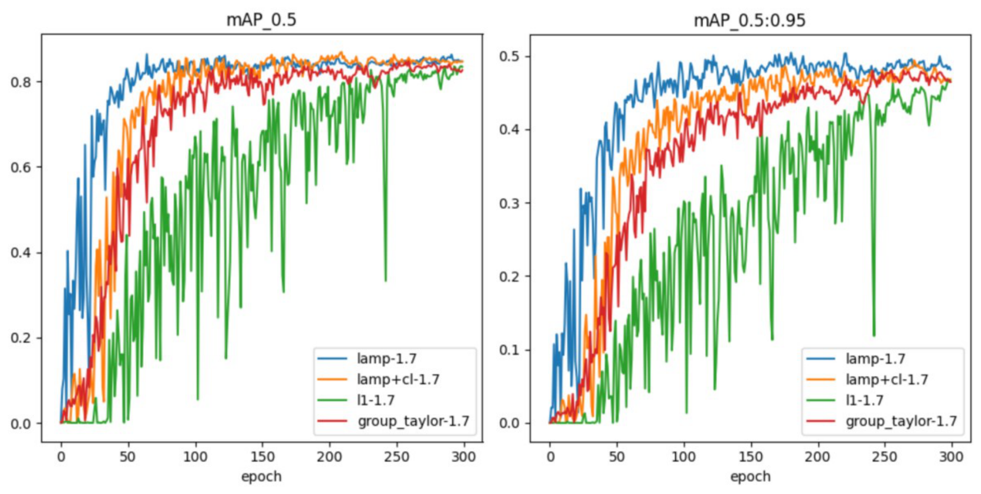
Table 5 and Figure 15 compare the effects of the evaluated pruning methods. At the 1.7× setting, LAMP alone achieves 84.6% $mA{P}_{0.5}$, 35.5 GFLOPs, 12.93 million parameters, and 54.3 FPS. Adding channel pruning reduces GFLOPs to 34.1 and the parameter count to 12.77 million, while increasing the inference rate to 59.4 FPS. Relative to LAMP alone, this additional stage reduces GFLOPs by 3.9% and increases FPS by 9.4%, with a decrease of 0.6 percentage points in $mA{P}_{0.5}$. These results quantify the additional efficiency provided by structured channel pruning under the tested configuration.

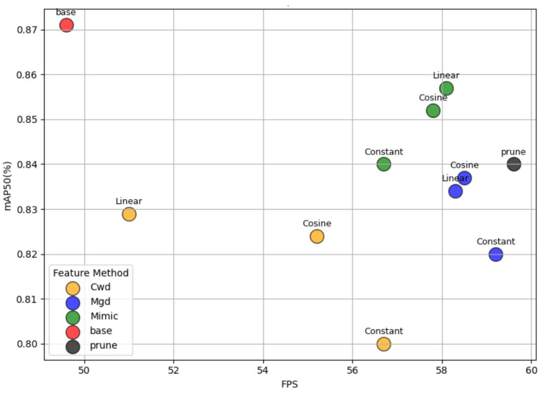
In the distillation experiments, Mimic, MGD, and CWD feature-distillation methods were paired with Constant, Cosine, and Linear loss-decay schedules using the LAMP + Cl model at the 1.7× pruning setting. Figure 16 summarizes the results. The uncompressed model shown by the red circle achieves 87.1% $mA{P}_{0.5}$ at 49.6 FPS, whereas the pruned model shown by the black circle achieves 84.0% $mA{P}_{0.5}$ at 59.4 FPS. Mimic + Linear distillation increases $mA{P}_{0.5}$ from 84.0% to 85.7%, while FPS decreases from 59.4 to 58.1. Thus, relative to the pruned model, distillation recovers 1.7 percentage points in $mA{P}_{0.5}$ with a 2.2% reduction in FPS. Relative to the uncompressed model, the final distilled model increases FPS by 17.1% while limiting the $mA{P}_{0.5}$ decrease to 1.4 percentage points.

3.5. Field Validation: 3D Positioning Accuracy Under Static Conditions

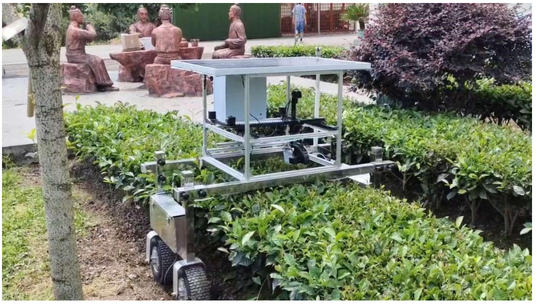
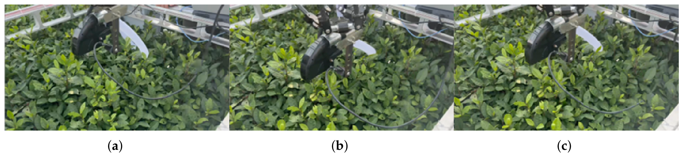
The field experiments were conducted at the tea gardens of the Chuan Tea Group (Figure 17). The robot used the compressed COS-DETR model, obtained by LAMP with channel pruning and Mimic + Linear knowledge distillation, as its visual perception system for acquiring real-time detection coordinates of premium tea buds. Based on the disparity maps from the stereo camera, the SGBM algorithm [32] computed the three-dimensional coordinates of each bud in the world coordinate system, which then guided the trajectory planning of the robotic arm. Finally, a Delta parallel manipulator drove the end effector to perform the approaching, grasping, separating, and collecting actions in sequence. The harvesting procedure is illustrated in Figure 18.

The evaluation reported in this subsection is limited to static positioning. Each of the 15 trials involved a single target and was performed with the platform stationary: the manipulator was commanded to the transformed coordinates, and the resulting position error was recorded. Continuous dynamic picking, in which the platform advances along the tea hedge while multiple targets are detected, localized, and picked in sequence, was not performed. The harvesting platform is still at the experimental prototype stage, and its perception, control, and actuation subsystems have not yet been integrated into a configuration capable of sustained continuous operation. Consequently, the picking success rate, the missed-detection rate, and the operation efficiency under dynamic picking conditions were not measured in this study, and the results reported below characterize three-dimensional positioning accuracy for stationary targets only.

Table 6. Three-dimensional positioning results under static field conditions ($n=15$).

No.	Actual Coords (mm)	Transformation Coords (mm)	Abs. Error (mm)	Rel. Error (%)
1	$(-210.4,-131.7,521.9)$	$(-213.1,-134.2,518.7)$	4.88	0.84
2	$(-223.8,-21.1,524.5)$	$(-225.5,-23.7,522.1)$	3.93	0.69
3	$(-25.5,-135.2,528.3)$	$(-23.8,-137.1,525.8)$	3.57	0.65
4	$(196.0,62.1,530.8)$	$(197.3,61.5,527.9)$	3.23	0.57
5	$(-209.1,112.5,505.0)$	$(-210.8,114.7,502.3)$	3.88	0.69
6	$(-168.9,-175.4,523.0)$	$(-167.7,-173.6,521.5)$	2.63	0.46
7	$(143.5,-227.6,527.3)$	$(142.9,-225.8,523.9)$	3.89	0.66
8	$(88.2,231.9,527.4)$	$(88.3,230.8,525.9)$	1.86	0.32
9	$(253.9,-76.1,516.3)$	$(254.7,-78.0,519.6)$	3.89	0.67
10	$(43.3,-374.7,524.6)$	$(43.7,-375.3,527.4)$	2.89	0.45
11	$(142.6,-388.3,522.0)$	$(142.3,-386.2,525.4)$	4.01	0.60
12	$(-241.4,371.8,518.7)$	$(-241.2,370.9,521.9)$	3.33	0.49
13	$(-316.7,184.5,509.1)$	$(-315.5,182.9,511.6)$	3.20	0.51
14	$(128.5,312.3,532.6)$	$(127.2,314.6,530.2)$	3.57	0.57
15	$(-319.1,309.3,525.6)$	$(-321.2,307.3,522.2)$	4.47	0.65

lists the 15 positioning trials, with the actual measured coordinates, the transformed coordinates from the camera, and the absolute and relative errors. The actual coordinates were recorded by the feedback coordinate system of a high-precision servo motor encoder, which serves as the reference baseline; this system records the three-dimensional coordinates of the end effector in real time as the arm reaches the picking point. The transformed coordinates were obtained after detecting the tea buds and applying the coordinate transformation. The absolute error measures the positioning accuracy over the whole workspace and is defined in Equation (32). The relative error normalizes the absolute error by the distance of the actual point from the origin, as shown in Equation (33).

$$\begin{array}{c}\hfill \begin{array}{c}\hfill {\mathsf{\Delta }}_{total}=\sqrt{{\left(x_1-x\right)}^2+{\left(y_1-y\right)}^2+{\left(z_1-z\right)}^2}\end{array}\end{array}$$

(32)

$$\begin{array}{c}\hfill \begin{array}{c}\hfill {\delta }_{total}={\displaystyle \frac{{\mathsf{\Delta }}_{total}}{\sqrt{x^2+y^2+z^2}}}\times 100\%.\end{array}\end{array}$$

(33)

Across the 15 static positioning trials, the absolute errors ranged from 1.86 to 4.88 mm with a mean of 3.55 mm, and the relative errors ranged from 0.32% to 0.84% with a mean of 0.59%. All absolute errors therefore remained below 5 mm under the tested static field conditions. These values characterize the accuracy with which a single detected bud can be localized and reached while the platform is stationary. Continuous dynamic picking was not performed in this study.

4. Discussion

4.1. Synergy of Multi-Scale and Frequency-Domain Features

The attention scheme and feature reconstruction in RT-DETR provide a reasonable starting point, but they do not fully capture the texture and scale diversity of tea fields. Premium tea buds have fine textures, large-scale differences across growth stages, frequent occlusion from bud clustering, and complex background interference. These characteristics weaken the baseline model’s multiscale feature representation and its adaptability to changing scenes, which limits the recognition accuracy needed for reliable robotic harvesting. Four modules were added to the backbone to address this gap. The Faster CGLU block strengthens the interaction among nonlinear features and gives the model richer representational capacity. Because tea buds exhibit textures at varied orientations and scales, the OmniKernel module uses kernels of different orientations and sizes to adapt to targets regardless of their pose and scale. FSAM works in both the frequency and spatial domains: the frequency branch captures global context, and the spatial branch preserves local edge and texture detail, connecting whole-image scene understanding with fine discrimination between buds and foliage. Finally, SPDConv partitions each feature map into spatial subregions and fuses them along the channel axis, which extends long-range consistency at little additional cost.

Table 2 reports a cumulative ablation rather than a full factorial analysis. Starting from the RT-DETR-R18 baseline at 84.6% $mA{P}_{0.5}$, the Faster CGLU stage raised the value to 85.9%. The complete OmniKernel stage, including its internal FSAM branch, further raised $mA{P}_{0.5}$ to 86.8%, and the SPDConv stage raised it to 87.1%. These increments match the intended complementary roles of the four modules on the tested tea bud dataset. The 0.9-percentage-point increment from 85.9% to 86.8% therefore remains attributable to the complete OmniKernel stage, including FSAM, rather than to FSAM alone. The separate control in Group 5 of Table 2 addresses the contribution of FSAM directly: disabling this branch inside the complete model lowered $mA{P}_{0.5}$ from 87.1% to 86.6%, a decrease of 0.5 percentage points.This control removes a single branch from the complete architecture, so it quantifies the marginal contribution of FSAM within the full model and does not separate the interactions between FSAM and the remaining OmniKernel branches or the behaviour of this branch when used on its own; a full branch-level factorial design would be required for that finer attribution and remains outside the scope of the present study.

4.2. Balancing Accuracy and Efficiency for Edge Deployment

The compression results show a measurable tradeoff between detection accuracy and deployment efficiency. The uncompressed COS-DETR achieved 87.1% $mA{P}_{0.5}$, 54.4 GFLOPs, 16.02 million parameters, and 49.6 FPS. At the 1.7× pruning setting, LAMP combined with channel pruning reduced the computational cost to 34.1 GFLOPs and the parameter count to 12.77 million, raised the inference rate to 59.4 FPS, and lowered $mA{P}_{0.5}$ to 84.0%. The compressed model was therefore 19.8% faster than the uncompressed model but lost 3.1 percentage points of $mA{P}_{0.5}$.

Mimic + Linear knowledge distillation partially compensated for this accuracy loss, raising $mA{P}_{0.5}$ from 84.0% to 85.7% while the inference rate changed from 59.4 to 58.1 FPS. The final model kept a 17.1% speed gain over the uncompressed model, together with reductions of 20.3% in parameters and 37.3% in GFLOPs, at the cost of 1.4 percentage points of $mA{P}_{0.5}$. Distillation therefore recovered part, but not all, of the accuracy removed by pruning. This final configuration is a compromise oriented toward deployment for the evaluated dataset, pruning ratio, and edge platform, and it should not be read as optimal for other hardware or operating conditions.

4.3. Comparison with Recent Tea-Detection Studies

Recent tea-detection studies have increasingly addressed small targets, complex backgrounds, variable illumination, and lightweight deployment. Wang et al. [33] introduced dynamic upsampling, pyramid compression attention, and spatial-channel reconstruction into YOLOv8. Tang et al. [34] combined CBAM, BiFPN, and Focal Loss to improve tea-bud detection under complex field conditions. Liu et al. [35] incorporated SOSA and LCA modules into YOLOv11 to strengthen feature extraction while controlling model complexity. Wang et al. [36] combined MobileViT Block, C2PSA, and depthwise separable convolution for lightweight tea instance segmentation. More recently, Zhang et al. [37] proposed a transformer-based path-fusion detector and evaluated tea-bud detection across different illumination conditions, cultivars, and growth stages, including validation on external datasets.

COS-DETR differs from these studies by combining RT-DETR-style feature modeling with structured pruning, knowledge distillation, and deployment on a tea-harvesting platform. On the dataset and evaluation protocol of this study, COS-DETR achieved higher $mA{P}_{0.5}$ than all evaluated YOLO and RT-DETR baselines, and its $mA{P}_{0.5:0.95}$ exceeded those of the standard models while remaining below those of the three small-scale configurations (Table 3). The additional three-scene comparison under backlighting, viewpoint variation, and background clutter suggests better detection under the sampled challenging conditions. However, the small number of scenes limits the strength of this environmental comparison and does not establish generalization to all lighting or plantation conditions.

A direct numerical ranking against published studies would be inappropriate because these studies used different tea cultivars, datasets, annotation criteria, image resolutions, data partitions, hardware platforms, and inference protocols. The present results therefore support an internally controlled comparison and demonstrate a favorable balance between accuracy and efficiency under the tested conditions. Broader conclusions will require external evaluation on datasets covering multiple cultivars, regions, and seasons under standardized protocols.

Compared with the above studies, COS-DETR contributes at three levels: detection architecture, model compression, and robotic integration. First, COS-DETR achieved the highest precision, recall, and $mA{P}_{0.5}$ among the evaluated configurations, although its $mA{P}_{0.5:0.95}$ was lower than those of YOLOv8s, YOLO11s, and YOLO12s. Second, LAMP with channel pruning and Mimic + Linear distillation produced a compact model with a favorable measured balance between accuracy and throughput on the NVIDIA Jetson Orin NX. Third, the static field positioning trials confirmed that the compressed detector can be integrated with stereo positioning and manipulator trajectory generation. Together, these results demonstrate the feasibility and practical value of the proposed system under the studied conditions. Further external testing across acquisition sessions and plantations, together with continuous harvesting trials, is required to assess deployment beyond the present dataset.

4.4. Limitations and Future Work

The present dataset was collected from specific tea cultivars at a single plantation, and each original image was acquired from a distinct tea plant. Source-image grouping kept each original image and its retained augmented versions within a single subset, which prevents trivial leakage between subsets. Within this experimental scope, COS-DETR showed strong comparative performance across the evaluated conditions. Whether this performance transfers to other cultivars, cultivation practices, canopy structures, and environmental conditions remains to be tested in future studies across multiple regions and seasons.

The field validation focused on 3D positioning accuracy and involved a limited number of trials. All 15 trials were static: the platform remained stationary, the manipulator was commanded to a single target, and no continuous dynamic picking was performed. The main reason is that the harvesting platform is still at the experimental prototype stage, and its perception, control, and actuation subsystems have not yet been integrated into a configuration capable of sustained continuous operation. The two core metrics requested for dynamic picking scenarios, namely the picking success rate and the missed-detection rate, were therefore not measured in this study, and the reported positioning accuracy describes stationary single-target positioning rather than performance during continuous harvesting. Nevertheless, the demonstrated integration of tea bud detection, stereo positioning, and manipulator control provides a practical foundation for further system development. Future continuous harvesting trials on a platform that reaches the required degree of subsystem integration will report the picking success rate, missed-detection rate, false-detection rate, harvest-cycle duration, fresh-leaf integrity, and long-term system stability.

5. Conclusions

COS-DETR, a lightweight tea bud detector based on RT-DETR, integrates the Faster CGLU block, the OmniKernel module with its internal FSAM, and SPDConv to model nonlinear feature interactions, textures at multiple scales, frequency and spatial context, and spatially rearranged features. On the held-out test subset defined by source-image grouping, COS-DETR achieved an $mA{P}_{0.5}$ of 87.1%, the highest value among the evaluated comparison models under the same test protocol.

For embedded deployment, LAMP with channel pruning reduced the parameter count by 20.3% and the GFLOPs by 37.3%. Mimic + Linear distillation then produced a final $mA{P}_{0.5}$ of 85.7% at 58.1 FPS on the NVIDIA Jetson Orin NX. The compressed model was integrated with an Intel RealSense D405 camera and a Delta manipulator to evaluate the detection, positioning, and control pipeline on the embedded platform. In 15 static field positioning trials, the integrated pipeline achieved absolute positioning errors below 5 mm, which confirms millimeter-level accuracy of the vision-guided positioning chain under real field conditions. These trials were performed with the platform stationary, because the harvesting platform is still an experimental prototype; continuous dynamic picking was therefore not carried out, and the picking success rate and the missed-detection rate under dynamic conditions are not reported in this study.

Overall, these results demonstrate the feasibility and practical value of combining lightweight tea bud detection with embedded robotic integration under the tested conditions, and they provide a technical foundation for broader field deployment and future commercial tea-harvesting applications. Future work will extend the evaluation to previously unseen plants, acquisition sessions, cultivars, and regions, and to long-duration harvesting operations, together with quantization, TensorRT acceleration, multisensor fusion, and joint optimization of hardware and software.

References

1. Liu, Z. The development process and trend of Chinese tea comprehensive processing industry. J. Tea Sci. 2019, 39, 115–122. [Google Scholar] [CrossRef]
2. Jia, J.; Wang, D.; He, L.; Wu, C.; Chen, J.; Zhang, J.; Li, Y. Research progress and prospects of mechanical technology for whole machine of high-quality tea picking robot. Trans. Chin. Soc. Agric. Mach. 2025, 56, 193–206. [Google Scholar] [CrossRef]
3. Song, R.; Gao, C. Application of computer image processing technology in tea picking robot system. J. Agric. Mech. Res. 2023, 45, 177–179+183. [Google Scholar] [CrossRef]
4. Tao, H.; Zhang, R.; Zhang, L.; Zhang, D.; Yi, T.; Wu, M. Tea harvest robot navigation path generation algorithm based on semantic segmentation using a visual sensor. Electronics 2025, 14, 988. [Google Scholar] [CrossRef] [Scilit]
5. Jia, J.; Li, Y.; Wang, X.; Yu, T.; Chen, J.; Zhou, Y.; Wu, C. Collaborative motion planning for multi-arm tea-picking robots. Comput. Electron. Agric. 2026, 244, 111470. [Google Scholar] [CrossRef] [Scilit]
6. Zhang, Y.; Yu, J.; Chen, Y.; Yang, W.; Zhang, W.; He, Y. Real-time strawberry detection using deep neural networks on embedded system (rtsd-net): An edge AI application. Comput. Electron. Agric. 2022, 192, 106586, Corrigendum in Comput. Electron. Agric. 2023, 215, 108445. [Google Scholar] [CrossRef] [Scilit]
7. Tang, Z.; Fang, L.; Sun, S.; Gong, Y.; Li, Q. ML-DETR: Multiscale-lite detection transformer for identification of mature cherry tomatoes. IEEE Trans. Instrum. Meas. 2025, 74, 2547018. [Google Scholar] [CrossRef] [Scilit]
8. Wang, H.; Luo, H.; Ren, L.; Huo, M.; Jiang, Y.; Kaynak, O. Data-driven design of distributed monitoring and optimization system for manufacturing systems. IEEE Trans. Ind. Inform. 2024, 20, 9455–9464. [Google Scholar] [CrossRef] [Scilit]
9. Wang, H.; Luo, H.; Qiao, X.; Huo, M.; Xu, X. Data-driven distributed robust monitoring and control optimization for interconnected systems. IEEE Trans. Ind. Inform. 2025, 21, 1399–1408. [Google Scholar] [CrossRef] [Scilit]
10. Bac, C.W.; van Henten, E.J.; Hemming, J.; Edan, Y. Harvesting robots for high-value crops: State-of-the-art review and challenges ahead. J. Field Robot. 2014, 31, 888–911. [Google Scholar] [CrossRef] [Scilit]
11. Arad, B.; Balendonck, J.; Barth, R.; Ben-Shahar, O.; Edan, Y.; Hellström, T.; Hemming, J.; Kurtser, P.; Ringdahl, O.; Tielen, T.; et al. Development of a sweet pepper harvesting robot. J. Field Robot. 2020, 37, 1027–1039. [Google Scholar] [CrossRef] [Scilit]
12. Rajendran, V.; Debnath, B.; Mghames, S.; Mandil, W.; Parsa, S.; Parsons, S.; Ghalamzan-E., A. Towards autonomous selective harvesting: A review of robot perception, robot design, motion planning and control. J. Field Robot. 2024, 41, 2247–2279. [Google Scholar] [CrossRef] [Scilit]
13. Yang, L. Fiber optic connector end-face defect detection based on machine vision. Opt. Fiber Technol. 2025, 91, 104158. [Google Scholar] [CrossRef] [Scilit]
14. Yang, L.; Xu, Q.; Liao, M.; Sun, K.; Xiang, R.; Xu, H. Feature selection based on information entropy for accurate detection of optical fiber end-face defects. Entropy 2026, 28, 462. [Google Scholar] [CrossRef] [Scilit]
15. Dong, C.; Wu, W.; Han, C.; Zeng, Z.; Tang, T.; Liu, W. Plucking point and posture determination of tea buds based on deep learning. Agriculture 2025, 15, 144. [Google Scholar] [CrossRef] [Scilit]
16. Zhang, C.; Wang, J.; Lu, G.; Fei, S.; Zheng, T.; Huang, B. Automated tea quality identification based on deep convolutional neural networks and transfer learning. J. Food Process Eng. 2023, 46, e14303. [Google Scholar] [CrossRef] [Scilit]
17. Yan, C.; Chen, Z.; Li, Z.; Liu, R.; Li, Y.; Xiao, H.; Lu, P.; Xie, B. Tea sprout picking point identification based on improved DeepLabV3+. Agriculture 2022, 12, 1594. [Google Scholar] [CrossRef] [Scilit]
18. Zhang, C.; Wang, J.; Yan, T.; Lu, X.; Lu, G.; Tang, X.; Huang, B. An instance-based deep transfer learning method for quality identification of Longjing tea from multiple geographical origins. Complex Intell. Syst. 2023, 9, 3409–3428. [Google Scholar] [CrossRef] [Scilit]
19. Yang, J.; Chen, Y. Tender leaf identification for early-spring green tea based on semi-supervised learning and image processing. Agronomy 2022, 12, 1958. [Google Scholar] [CrossRef] [Scilit]
20. Wang, Y.; Ren, Y.; Kang, S.; Yin, C.; Shi, Y.; Men, H. Identification of tea quality at different picking periods: A hyperspectral system coupled with a multibranch kernel attention network. Food Chem. 2024, 433, 137307. [Google Scholar] [CrossRef] [Scilit]
21. Yang, G.; Weng, D.; Li, Z.; Wu, Y. Tomato ripeness detection model based on improved RT-DETR lightweight model. Agronomy 2026, 16, 932. [Google Scholar] [CrossRef] [Scilit]
22. Wang, H.; Gu, J.; Wang, M. A review on the application of computer vision and machine learning in the tea industry. Front. Sustain. Food Syst. 2023, 7, 1172543. [Google Scholar] [CrossRef] [Scilit]
23. Shi, D. TransNeXt: Robust foveal visual perception for vision transformers. In Proceedings of the 2024 IEEE/CVF Conference on Computer Vision and Pattern Recognition (CVPR), Seattle, WA, USA, 16–22 June 2024; IEEE: New York, NY, USA, 2024; pp. 17773–17783. [Google Scholar] [CrossRef] [Scilit]
24. Cui, Y.; Ren, W.; Knoll, A. Omni-kernel modulation for universal image restoration. IEEE Trans. Circuits Syst. Video Technol. 2024, 34, 12496–12509. [Google Scholar] [CrossRef] [Scilit]
25. Sunkara, R.; Luo, T. No more strided convolutions or pooling: A new CNN building block for low-resolution images and small objects. In Machine Learning and Knowledge Discovery in Databases, Proceedings of the European Conference, ECML PKDD 2022, Grenoble, France, 19–23 September 2022; Lecture Notes in Computer Science; Springer: Cham, Switzerland, 2023; Volume 13715, pp. 443–459. [Google Scholar] [CrossRef] [Scilit]
26. Chen, L.; Zhang, H.; Xiao, J.; Nie, L.; Shao, J.; Liu, W.; Chua, T.S. SCA-CNN: Spatial and channel-wise attention in convolutional networks for image captioning. In Proceedings of the 2017 IEEE Conference on Computer Vision and Pattern Recognition (CVPR), Honolulu, HI, USA, 21–26 July 2017; IEEE: New York, NY, USA, 2017; pp. 6298–6306. [Google Scholar] [CrossRef] [Scilit]
27. Zhu, M.; Gupta, S. To prune, or not to prune: Exploring the efficacy of pruning for model compression. arXiv 2017, arXiv:1710.01878. [Google Scholar] [CrossRef] [Scilit]
28. Polyak, A.; Wolf, L. Channel-level acceleration of deep face representations. IEEE Access 2015, 3, 2163–2175. [Google Scholar] [CrossRef] [Scilit]
29. Aghli, N.; Ribeiro, E. Combining weight pruning and knowledge distillation for CNN compression. In Proceedings of the 2021 IEEE/CVF Conference on Computer Vision and Pattern Recognition Workshops (CVPRW), Virtual Event, 19–25 June 2021; IEEE: New York, NY, USA, 2021; pp. 3185–3192. [Google Scholar] [CrossRef] [Scilit]
30. Liu, D.; Zhu, Y.; Liu, Z.; Liu, Y.; Han, C.; Tian, J.; Li, R.; Yi, W. A survey of model compression techniques: Past, present, and future. Front. Robot. AI 2025, 12, 1518965. [Google Scholar] [CrossRef] [Scilit]
31. Hinton, G.; Vinyals, O.; Dean, J. Distilling the knowledge in a neural network. arXiv 2015, arXiv:1503.02531. [Google Scholar] [CrossRef] [Scilit]
32. Hirschmüller, H. Accurate and efficient stereo processing by semi-global matching and mutual information. In Proceedings of the 2005 IEEE Computer Society Conference on Computer Vision and Pattern Recognition (CVPR’05), San Diego, CA, USA, 20–26 June 2005; IEEE: New York, NY, USA, 2005; Volume 2, pp. 807–814. [Google Scholar] [CrossRef] [Scilit]
33. Wang, C.; Li, H.; Deng, X.; Liu, Y.; Wu, T.; Liu, W.; Xiao, R.; Wang, Z.; Wang, B. Improved You Only Look Once v.8 model based on deep learning: Precision detection and recognition of fresh leaves from Yunnan large-leaf tea tree. Agriculture 2024, 14, 2324. [Google Scholar] [CrossRef] [Scilit]
34. Tang, X.; Tang, L.; Li, J.; Guo, X. Enhancing multilevel tea leaf recognition based on improved YOLOv8n. Front. Plant Sci. 2025, 16, 1540670. [Google Scholar] [CrossRef] [Scilit]
35. Liu, Z.; Zhuo, L.; Dong, C.; Li, J.; Li, Y. TBD-Y: Automatic tea bud detection with synergistic object-spatial attention and global-local attention guided feature fusion. Smart Agric. Technol. 2025, 12, 101066. [Google Scholar] [CrossRef] [Scilit]
36. Wang, W.; Xi, Y.; Gu, J.; Yang, Q.; Pan, Z.; Zhang, X.; Xu, G.; Zhou, M. YOLOv8-TEA: Recognition method of tender shoots of tea based on instance segmentation algorithm. Agronomy 2025, 15, 1318. [Google Scholar] [CrossRef] [Scilit]
37. Zhang, T.; Yang, Q.; Tong, X.; Hu, L.; Shao, J. A transformer-based path fusion detector network for tea bud detection. Smart Agric. Technol. 2026, 14, 102321. [Google Scholar] [CrossRef] [Scilit]
Figure 1. The distribution of Chuan Tea Group’s tea plantation.
Processes 14 02963 g001
Figure 2. Six dataset types: (a) Overhead image of tea leaves. (b) Left-oblique image of tea leaves. (c) Right-oblique image of tea leaves. (d) Back-lit image of tea leaves. (e) Front-lit image of tea leaves. (f) Multi–tea leaf environment image.
Processes 14 02963 g002
Figure 3. Data augmentation: (a) Original image. (b) Horizontal flipping. (c) Random rotation. (d) Brightness reduction. (e) Brightness enhancement. (f) Gaussian blurring. (g) Random cropping. (h) Affine transformations. (i) Noise addition.
Processes 14 02963 g003
Figure 4. Tea-harvesting robot.
Processes 14 02963 g004
Figure 5. COS-DETR model architecture diagram. S2/S3/S4: stage 2/3/4 features; AIFI: attention-based intra-scale feature interaction; F5: the fifth (deepest) backbone feature map; Csp: cross-stage partial residual structure; Conv: convolution; s: stride; Upsamp: upsampling; RepC3: reparameterizable C3 module.
Processes 14 02963 g005
Figure 6. BasicBlock Faster CGLU Module. In: input; Conv: convolution; ReLu: rectified linear unit; Max-Pool: max pooling; Faster_CGLU: speed-optimized convolutional gated linear unit module; Out: output.
Processes 14 02963 g006
Figure 7. Faster CGLU module.
Processes 14 02963 g007
Figure 8. OmniKernel module. Conv: convolution; DConv: depthwise convolution; ⊕: element-wise feature addition; Local: local; Large: large-scale; Global: global; FSAM: Frequency–Spatial Attention Module; DCAM: dual-channel attention module.
Processes 14 02963 g008
Figure 9. FSAM. Input: input; Conv: convolution; FFT: fast Fourier transform; ⊙: element-wise multiplication; IFFT: inverse fast Fourier transform; ABS: absolute value; Output: output.
Processes 14 02963 g009
Figure 10. Hybrid Pruning Flowchart. a1, a2, a3: normalization factors for different network layers; orange blocks: feature maps; yellow blocks: weights; transparent regions with dashed outlines: pruned portions; solid connections: forward propagation paths; downward dashed arrows: subsequent channel pruning; gray background: LAMP pruning; blue background: channel pruning.
Processes 14 02963 g010
Figure 11. Knowledge Distillation. Teacher: teacher network; Student: student network; Soft labels: teacher network predictions; Hard labels: ground-truth annotations; gray stacked blocks: schematic network architecture.
Processes 14 02963 g011
Figure 12. Ablation study mAP comparison map.
Processes 14 02963 g012
Figure 13. Comparison of tea-bud detection mAP for different models.
Processes 14 02963 g013
Figure 14. Tea leaf recognition detection results: (a) COS-DETR. (b) RT-DETR-R18. (c) YOLOv8. (d) YOLOv5.
Processes 14 02963 g014
Figure 15. Comparison of Pruning mAP Results.
Processes 14 02963 g015
Figure 16. Experimental Results of Different Distillation Methods.
Processes 14 02963 g016
Figure 17. Field Tea-Harvesting Experiment.
Processes 14 02963 g017
Figure 18. Picking process diagram: (a) the approaching; (b) the grasping; (c) the collecting actions.
Processes 14 02963 g018