


Abstract
Large language models (LLMs) are increasingly embedded in control-design workflows, yet their ability to compare candidate controllers remains uncertain. A simulator-grounded performance-judgment benchmark evaluates four open-weight checkpoints across a quadruple-tank process, a recycle reactor, and a synthetic 3-by-3 cyclic plant. Declarative control-theory accuracy is nearly saturated (98–100% pooled by plant), whereas qualitative-description accuracy for ranking PI gain sets is 46.8%, 31.8%, and 53.2%, respectively. Outputs are associated with lower gain magnitudes, but the association varies with scaling, plant, and controller sampling. Across 271 replay-stable pairs, IAE rankings agree with ISE rankings on 95.2%; under a combined simulator perturbation, 88.7% of seed–item labels are preserved. On fixed gain pairs, equations and 14-point response trajectories raise pooled accuracy only from 46.8% to 51.2% and 51.0%. All 12 prespecified trajectory-versus-qualitative intervals include zero, and none survives Holm correction. Swapping displayed trajectory values changes 9.5% of parsed choices. By contrast, a numerical scaffold derived from the same samples raises evidence-consistent accuracy from 51.1% to 88.1%, with 11 of 12 contrasts surviving Holm correction. The main bottleneck under these prompts is extracting and aggregating raw numerical evidence, not the final comparison alone. This result does not identify a unique mechanism or establish a general absence of dynamic reasoning. Simulator-based validation remains necessary before LLM judgments are used for controller tuning.
1. Introduction
Tuning feedback controllers for strongly coupled multi-input multi-output (MIMO) process plants is difficult because loop interactions make the effect of an individual gain plant dependent. Recent work inserts large language models (LLMs) into this loop to propose gains, interpret requirements, and coordinate external optimization and simulation [1,2]. These workflows can benefit from language-based structural knowledge without requiring the LLM itself to be a numerical simulator. However, when an LLM is asked to rank candidate controllers, the workflow implicitly relies on a narrower capability: the model must use the information in its prompt to discriminate plant-specific closed-loop outcomes. That comparative capability should be measured separately from end-to-end tuning success.
The stakes are especially high in control applications. A mis-tuned multivariable loop can oscillate, saturate actuators, or become unstable, while a fluent explanation can make an incorrect recommendation appear credible. It therefore matters whether an open-weight LLM can discriminate coupled closed-loop outcomes from the information supplied. It also matters which observable rules are associated with its choices and how those associations change across plants and gain scalings. This study measures forced-choice behavior, not token-level confidence or latent model states.
The benchmark studies locally deployable, open-weight checkpoints, which can keep process data inside an organization’s infrastructure. The baseline gives each model a qualitative description of coupling, sign, and set-point conflict together with concrete PI gain candidates. A matched-item intervention then adds either the complete equations or sampled closed-loop trajectories. This separation tests both performance judgment under a realistic qualitative-information constraint and whether specific dynamical information produces a measurable recovery.
Across the three tested plants, declarative control knowledge is nearly saturated, whereas pairwise performance judgment varies substantially across models and plants. When pooled by plant, choices favor lower gain magnitude under both raw and dimension-normalized definitions. The checkpoint-level breakdown reveals substantial exceptions to this aggregate pattern (Section 4.7).
This paper makes three contributions:
- (1)
- This study introduces a simulator-grounded performance-judgment benchmark. It contains 196 unique items per model for the quadruple-tank and cyclic plants and 166 for the reactor.
- (2)
- The analysis audits parse coverage, label balance, model-level performance, and observable gain-magnitude rules. The analysis remains behavioral and does not infer unobserved internal mechanisms.
- (3)
- This study tests major protocol threats through a controller-form correction, independently resampled pools, an equal-budget feedback ablation, and matched-item information interventions. The complete evidence chain is reported here without importing performance claims from another study.
Figure 1 summarizes the complete study narrative, from simulator-grounded benchmark construction to the diagnosis of raw numerical evidence use and the resulting simulator-verified workflow recommendation.
Figure 1.
Study story overview. Phase 1 constructs simulator-grounded performance-judgment probes and contrasts declarative control knowledge with plant-specific PI-gain ranking. Phase 2 checks simulator-label sensitivity and examines equations, sampled trajectories, trajectory-value swaps, and a numerical scaffold, then summarizes the recommended division of labor between qualitative LLM assistance and numerical verification.
2. Related Work
The relevant literature spans process-engineering LLM systems, capability evaluation, controller tuning, and predictive world models. These areas must be distinguished because an end-to-end system can succeed through retrieval, simulation, optimization, or verification even when the language model alone cannot reliably rank two numerical controllers.
2.1. LLMs in Process Engineering and Control-Design Workflows
Recent reviews organize engineering uses of LLMs around knowledge access, monitoring, simulation, optimization, and decision support [3,4,5]. The common design principle is bounded autonomy: the language model coordinates domain knowledge and tools, while numerical or symbolic components verify consequential outputs. Applied process systems instantiate this principle through retrieval-augmented question answering [6], scheduling optimization [7], digital-twin supervision [8], neuro-symbolic checks [9], and real-time batch-process decision support [10]. Recent articles in Processes also evaluate multimodal inspection and disassembly [11], photovoltaic fault diagnosis [12], and motor fault diagnosis and predictive maintenance [13]. In each case, the primary unit of evaluation is the complete architecture or its downstream task performance. These studies therefore do not establish that the LLM alone can compare fixed controllers from raw closed-loop evidence.
Control-oriented systems make the external computation explicit. SmartControl translates natural-language performance requirements into numerical targets, delegates PID search to numerical optimizers, and evaluates simulated step responses [1]. Ares-Milian et al. use an LLM for input–output pairing and stage definition within automated decentralized tuning [2]. A recent survey maps the growing interface between LLMs and control design and identifies empirical robustness, hardware validation, and computational constraints as open priorities [14]. Wen et al. evaluate direct and supervisory LLM use in a water-tank control framework and report that the constrained LLM–PID configuration is more viable than direct LLM control [15]. Schall confines LLM inference to an advisory layer and subjects proposed actions to deterministic, process-grounded verification [16]. These systems demonstrate useful ways to combine language models with control tools. They do not isolate whether a model’s choice responds causally to raw closed-loop numerical evidence when two gain sets are held fixed. That narrower construct is the target of the matched-item and trajectory-swap interventions.
2.2. Capability Evaluation and Operational Skill
ControlBench evaluates frontier LLMs on textbook control problems involving analysis and design [17]. It establishes control engineering as a meaningful technical-reasoning domain, but does not test two fixed gain vectors against plant-specific closed-loop outcomes. More generally, fluent recitation does not guarantee operational use of knowledge. Language competence can be dissociated from broader reasoning and world modeling [18], and planning benchmarks show that models may state domain rules yet fail to produce valid plans [19]. Critiques of scale similarly caution against equating statistical fluency with understanding [20].
Numerical and tabular benchmarks sharpen this concern. FinQA and TAT-QA require retrieval, arithmetic, and multi-step aggregation over mixed text–table evidence [21,22]. Broader studies show that table format, context length, and basic magnitude operations remain consequential sources of error [23,24,25,26]. Program-aided and tool-augmented methods improve reliability by separating language-based reasoning from exact computation [27,28,29]. The present benchmark is not another general table-question-answering task. It instead uses simulator labels and matched controller pairs to test whether the representation of the same closed-loop evidence changes a consequential engineering judgment.
The declarative and pairwise tasks are not difficulty matched. The former tests textbook knowledge, whereas the latter requires a plant-specific ranking from qualitative structure or sampled responses. The observed gap therefore shows that high declarative accuracy can coexist with weak performance judgment under the tested tasks; it does not quantify a difficulty-controlled difference or isolate a single latent capability. Simulator-derived labels and prespecified behavioral rules make the narrower comparison auditable.
2.3. Classical and Data-Driven Controller Tuning
Controller tuning traditionally couples a candidate controller to an explicit model or measured response. Relay auto-tuning, SIMC, and internal model control provide transparent single-loop procedures [30,31,32]. The relative gain array and multivariable feedback design address interaction and pairing directly [33,34]. Data-driven alternatives include iterative feedback tuning, model-free adaptive control, and reinforcement-learning search [35,36,37]. Recent PI and PI–PD optimization likewise evaluates candidates against explicit control criteria [38], while PC-Gym provides reproducible process environments for learning-based control [39].
These approaches differ in assumptions and optimization strategy, but all make performance evaluation an explicit computational step. The present question is orthogonal to which tuner is best: the benchmark tests an LLM asked to rank two concrete gain sets under controlled information conditions.
2.4. Forward and World Models
Model-based reinforcement learning learns a transition model and plans against predicted consequences [40]. World-model architectures similarly compress environment dynamics into a predictive latent representation [41]. A controller-tuning agent that reasons about dynamics must, explicitly or implicitly, estimate how a change in gains alters the closed-loop response.
The experiments do not attempt to recover an internal representation. Instead, the analysis tests observable consequences: discrimination from qualitative structure, response to added equations or trajectories, sensitivity to swapped trajectory values, and recovery after numerical aggregation. Failure on these probes does not establish that an internal dynamics representation is absent. It bounds how reliably the tested prompts and checkpoints convert available evidence into a controller ranking.
3. Materials and Methods
3.1. Plants and the Closed-Loop Cost
The benchmark uses three strongly coupled MIMO process simulators that differ in dimensionality, gain sign, and coupling topology. Their diversity provides three contrasting case studies but does not constitute a representative sample of all process plants. Each plant is controlled by decentralized PI loops in position form. For loop j with tracking error , the controller updates its integral state and saturates the resulting command:
The quadruple-tank and reactor implementations roll back the latest integral increment when saturation occurs; the synthetic cyclic plant retains the integral state. A controller is a vector of per-loop gains . The performance-judgment labels use integrated absolute error (IAE), computed by trapezoidal quadrature over the recorded samples for the tank and reactor. The discrete cyclic plant accumulates absolute tracking error at each post-update output, multiplied by . The exploratory tank-tuning ablation (Section 4.8) uses the penalized cost
where is the recorded pump command and N is the number of recorded samples. The total-variation penalty uses the fixed command scale 10, as in the P2 implementation. Appendix B gives the plant equations, parameters, initial conditions, horizons, set-points, and actuator limits.
The quadruple-tank [42] is a canonical non-minimum-phase benchmark that is also used in process-control learning environments [39]. Loop 1 gains drive pump 1, and loop 2 gains drive pump 2. The cross-coupling is asymmetric: raising lifts strongly and weakly, whereas raising lifts strongly and moderately. The set-points conflict ( up, down).
The series CSTR with recycle (cstr2) is a reactor in which coolant temperatures control outlet concentrations and . The process gains are negative: lowering coolant temperature raises the outlet concentration. A recycle stream couples the reactors, and the set-points conflict ( up, down).
The cyclic plant (mimo3) has dominant off-diagonal coupling. Each input chiefly drives a different output (, , ), so a competent controller must respect the cyclic rather than diagonal pairing. Its set-points conflict and switch at mid-horizon. Together, the plants span positive and negative gains, diagonal and cyclic coupling, and two- and three-loop dimensionality.
These cases were selected to expose gain-magnitude rules to different empirical relationships with performance. In the saved raw-scale pools, lower total gain is strongly misaligned with IAE ranking on the reactor, nearly neutral on the tank, and often aligned on the cyclic plant. Because these relationships were inspected on the same plants used for the behavioral analysis, the rule characterization is exploratory rather than a held-out mechanism test.
3.2. Gain Sampling and Ground Truth
For each plant, the benchmark draws a pool of candidate controllers. Each gain is sampled log-uniformly over a wide range—roughly two to three orders of magnitude—and the closed loop is simulated to obtain the cost. Concretely, and for the quadruple-tank. The reactor uses negative gains, with and drawn log-uniformly over and , respectively. The plant uses and on each of its three loops. Samples whose simulated cost is non-finite or exceeds a plant-specific cap are discarded. The retained IAE ranges are for the tank, for the reactor, and for the cyclic plant; the reactor range is therefore comparatively narrow. Item construction uses NumPy generator seed 20260611, and deterministic plant simulation uses seed 0 where the interface accepts a seed. All reported labels are preserved in the saved question files rather than regenerated during analysis.
3.3. Performance-Judgment Probe
Each model receives a qualitative plant description that specifies the coupling direction, gain sign where applicable, actuator range, and conflicting set-points. It then answers three families of forced-choice questions whose labels come from the simulator. The models do not receive complete equations, numerical plant parameters, or trajectories, so the construct is performance judgment from qualitative descriptions:
- Pairwise (E2-pairwise). Given two sampled controllers, which yields lower tracking error (IAE)? Up to such items per plant are built by drawing pairs from the pool and binning them by the ground-truth quality gap, defined as the IAE ratio : easy (), medium (), and hard (). The bins show whether accuracy improves when the correct answer is “obvious.” The tank and probes contain 100 pairs each. The reactor’s narrower IAE spectrum produces 74 medium/hard pairs and no easy bin.
- Direction. Starting from a sampled controller, one gain is multiplied by 3 or by with the others fixed; does the closed-loop IAE increase or decrease? The probe keeps items per plant for which the true change in IAE exceeds , balanced between increase and decrease.
- Tracking quality. Will a single sampled controller track the conflicting set-points well or poorly relative to the saved pool? The pool is labeled by a median split on IAE, followed by drawing balanced good/poor items per plant. This task does not measure closed-loop stability in the control-theoretic sense.
Table 1 separates the measured constructs and the associated claim boundaries. The pairwise probe is the primary endpoint because it directly matches controller selection, has a simulator-defined binary label, and reaches complete parser coverage. Direction and tracking quality are secondary format-sensitivity probes. E1 supplies a declarative reference but is not difficulty matched to E2. P3 and P4 test responses to particular information representations; neither intervention identifies a latent reasoning faculty.
Table 1.
Measured constructs and interpretation boundaries.
Figure 2 shows the retained controller-pool support and the resulting pairwise difficulty distribution. It makes explicit that the saved reactor probe contains only hard and medium pairs, whereas the cyclic plant spans a much broader range of performance separations.
Figure 2.
Benchmark-construction diagnostics. Panel (a) shows empirical cumulative distributions of the retained controller costs after normalization by the within-plant median ( controllers per plant). Panel (b) shows every saved pairwise IAE ratio; points are individual items, black segments are the interquartile ranges, and diamonds are medians. Blue, orange, and green denote the quadruple-tank, reactor, and cyclic plants, respectively. The vertical thresholds at and define hard, medium, and easy bins. The tank, reactor, and probes contain 100, 74, and 100 pairwise items, respectively.
All items are forced-choice with chance ; the model is instructed to reason briefly and to end with an explicit token (FINAL: A/B, UP/DOWN, or GOOD/BAD) parsed by a fixed rule. The overall design is summarized in Figure 3: the simulator supplies ground truth, the same plant description is given to the model, and the model’s forced-choice answers are scored against that ground truth.
Figure 3.
Performance-judgment probe. The simulator produces a saved 320-controller pool and IAE labels. Open-weight LLMs receive qualitative plant descriptions and answer pairwise, direction, tracking-quality, and declarative knowledge questions. Analysis reports model-level accuracy, parse coverage, label-balanced sensitivity, and agreement with prespecified behavioral rules.
The historical quadruple-tank description called the controller “velocity-form” even though the simulator implements position-form PI with integral-state rollback under saturation (Appendix B). A protocol-correction study (P0) reruns the same 100 pairwise, 40 direction, and 40 tracking-quality tank items per checkpoint after correcting only this controller-form metadata. Ground-truth labels and numerical gains are unchanged.
A representative pairwise item (quadruple-tank) reads:
“Set A: ; Set B: . Which yields lower tracking error?”
Here Set A (the asymmetric, higher-gain controller that emphasizes loop 1) is in fact better. A magnitude-based rule instead selects the numerically gentler Set B, illustrating how that observable rule can disagree with simulated ground truth.
3.4. Matched-Item Information Intervention
To separate missing plant information from failure to use available evidence, P3 reuses 50 saved pairwise items per plant under three conditions. The item, gain vectors, correct label, and decoding protocol are held fixed. The qualitative condition (Q) uses the original plant description. The equation condition (E) supplies the complete state equations, numerical parameters, initial condition, set-points, horizon, actuator bounds, controller pairing, and PI implementation, but no simulated response. The trajectory condition (T) retains the qualitative description and adds 14 common time points containing the reference and output vectors for Sets A and B. It provides neither the IAE values, the control commands, nor the correct option; the model must compare the sampled tracking errors. The conditions deliberately differ in the information supplied and are not token-count matched. P3 therefore estimates the effect of these concrete information packages, not a generic effect per added token. Mean prompt lengths are 715, 1079, and 1706 characters (105, 142, and 224 whitespace-delimited words) for Q, E, and T, respectively. Thus, prompt length remains part of the information-package contrast and is not excluded as an alternative explanation. No controlled estimate of context-window decay or positional sensitivity was collected. The saved inference code passes the complete formatted prompt to the tokenizer without requesting input truncation; the 192/512-token limits apply to generated output. However, preserving the input does not establish that every part of the context is used equally. The trajectory table has a fixed location after the plant description, with Set A preceding Set B; neither table location nor candidate order is counterbalanced. Appendix D reports the observed option frequencies separately from this unmeasured positional effect. Because all P3 conditions use a uniform two-sentence output constraint, Q is the within-P3 reference condition rather than an exact replication of the full E2 baseline.
Within each plant, the subset contains 25 A and 25 B labels. Selection seed 20260808 cycles across the available difficulty bins within each label. The saved prompts round gains to four decimal places, whereas the original labels use higher-precision pool values. Consequently, the rounded-gain replay changes the ordering of one tank item and two cyclic-plant items. These three candidates are excluded before subset selection; every retained replay preserves the saved label. All conditions use greedy decoding. The primary contrast is the paired accuracy change within each checkpoint–plant stratum. The analysis reports accuracy, balanced accuracy, parse coverage, paired bootstrap intervals (10,000 item resamples), and exact McNemar tests, with Holm correction across the 12 primary checkpoint–plant tests. and are secondary descriptive contrasts. The P3 parser first requires the requested FINAL token and otherwise accepts only an unambiguous terminal statement of the form “Set A/B yields lower tracking error”; raw token compliance is retained separately. The 62 outputs that still lacked an interpretable choice at the original 192-token cap were deterministically regenerated from the identical prompt with a 512-token cap. The latest attempt is analyzed; eight outputs remain unparsed, are scored incorrect in raw accuracy, and are also reflected in condition-specific coverage. A trapezoidal numerical oracle using only the 14 displayed rows recovers the saved ordering for 49/50 tank, 49/50 reactor, and 47/50 cyclic items (145/150, 96.7%). The sampled evidence is therefore highly, but not perfectly, sufficient for the original full-trajectory labels.
3.5. Causal Trajectory-Use and Numerical-Scaffold Audit
P4 asks a narrower question than P3: do model choices respond to the displayed trajectory values? It also tests whether the same checkpoints can use a reduced numerical representation of those values. P4 includes every saved pairwise item whose rounded gains reproduce the saved full-trajectory label: 99 tank, 74 reactor, and 98 cyclic-plant items (271 total). The four conditions reuse the same gain pair, qualitative description, question, and greedy decoding rule. Q is the qualitative reference. T adds the same 14 sampled reference and output rows as P3. X is a causal value-swap intervention: it preserves the T prompt format and question but exchanges the displayed Set A and Set B trajectory columns. S is a positive-control scaffold derived only from those 14 rows. It provides the trapezoidal absolute-error component for each output channel and states that the lower component sum is preferred, while withholding both totals and the final choice.
The full-trajectory simulator label remains the target for Q and for the naturalistic T accuracy contrast. For T, X, and S, an evidence label is additionally defined from trapezoidal integration of the displayed samples; X therefore reverses the T evidence label by construction, whereas S preserves it. Preflight checks verify matched item identities; T/X prompt, format identity; the intended evidence, label reversal; and invariance of the S answer after the displayed eight, significant-digit rounding. The sampled evidence label matches the saved full-trajectory label for 98/99 tank, 72/74 reactor, and 92/98 cyclic items (262/271, 96.7%).
P4 reports raw and label-balanced accuracy and parse coverage. The prespecified full-label contrast and evidence-label contrast use paired item bootstrap intervals (10,000 resamples) and exact McNemar tests, with separate Holm corrections across their 12 checkpoint–plant strata. A 90% bootstrap interval wholly contained within percentage points is treated as practical equivalence under the prespecified margin. For the T/X causal audit, the primary descriptive quantities are parsed-pair coverage, choice-flip rate, and persistence of the original choice. The analysis also reports how often both T and X choices follow their respective displayed evidence labels. X is intentionally an internally inconsistent counterfactual relative to the stated gains and is therefore interpreted only as an evidence-use intervention, not as a naturalistic controller-ranking condition.
3.6. Performance-Metric and Perturbation Sensitivity
The primary pairwise label is intentionally tied to cumulative tracking error, but controller quality is multidimensional. To quantify dependence on that choice, all 271 P4-eligible gain pairs are replayed under the nominal simulator. Five alternative summaries are computed from each full trace: integrated squared error (ISE), peak absolute tracking error, mean absolute error over the final 10% of samples, actuator-range-normalized total command variation , and a composite sensitivity score . Pairwise agreement with the saved IAE label is reported for each summary. The composite score is a cross-plant sensitivity measure and is distinct from the tank-only optimization objective J used in P2.
A second replay tests whether the nominal IAE labels are fragile to a combined simulation perturbation. Ten seeds apply (i) independent plant-parameter multipliers drawn with 5% standard deviation and clipped to , (ii) zero-mean measurement noise scaled to each output, (iii) one simulation-step actuation delay, and (iv) two fixed-time state disturbances. Parameter variation acts on pump and outlet coefficients in the tank, flow, recycle, heat-transfer, and reaction-rate coefficients in the reactor, and the gain matrix in the cyclic plant. Sets A and B share the same seed within each pair. The analysis reports nominal-label preservation and rescoring of the existing deterministic Q choices against the perturbed labels. This stress condition is a simulator-side sensitivity analysis, not a calibrated noise model or laboratory validation.
3.7. Control-Theory Knowledge Baseline
To place the performance-judgment results beside a declarative reference, this study administers a qualitative control-theory question set (E1). These items are answerable from textbook knowledge and the stated coupling. Examples ask whether higher proportional gain accelerates the response at the risk of overshoot and whether diagonal pairing is suitable for a plant with dominant off-diagonal coupling. E1 uses the same plant description and a forced-choice answer token, but it is neither information-matched nor difficulty-matched to comparing two numerical gain sets. The E1–pairwise contrast is therefore descriptive. It shows that high qualitative QA accuracy can coexist with weak performance judgment under the present prompts; it does not imply that the tasks isolate a single latent faculty.
3.8. Heuristic Reverse-Engineering
To characterize regularities in the forced choices, the answers are compared with a prespecified family of simple rules. These rules prefer the controller with lower raw total gain magnitude, lower proportional-gain magnitude, lower integral-gain magnitude, or greater proportional-gain symmetry. Because and have different numerical ranges, this study adds a scale-sensitivity analysis. For gain dimension j, let be the empirical cumulative distribution of in the saved 320-controller pool. The two magnitude summaries are
where d is the number of gain dimensions. The normalized score gives each dimension equal percentile weight within the sampled pool. Both summaries are applied to the same saved gains and model choices; normalization changes the analysis rule, not the values shown to the model. For each checkpoint and plant, the analysis reports raw and normalized rule-agreement rates and their difference in percentage points. It also reports the descriptive Spearman correlation between the signed margin and the binary choice indicator , using average ranks for ties. Positive correlation indicates that larger margins favoring the lower-magnitude Set A are associated with more A choices. There are no equal-magnitude candidate pairs under either summary in the baseline probe.
For each rule, consistency is the fraction of model choices that agree with the rule, whereas correctness is the fraction of simulated ground-truth labels that agree with it. These are behavioral associations and do not uniquely identify the model’s internal computation. To assess dependence on the sampled probe pairs, the analysis also enumerates all unordered controller pairs in each saved pool. This tests pair selection within the current log-uniform pools.
Sampling sensitivity (P1) is tested separately by generating new 320-controller pools under two prespecified designs. The first uses Latin-hypercube sampling in log-gain space over the original bounds. The second uses independent log-uniform sampling after removing the outer 10% of each log-gain range at both ends (the inner 80%). For each design and plant, three pool seeds (20260731–20260733) yield 50 label-balanced pairwise items per checkpoint. Reported quantities include checkpoint accuracy and agreement with the raw and percentile-normalized magnitude rules for each seed. The analysis also enumerates all 51,040 pairs in every new pool to characterize rule correctness independently of the selected questions.
3.9. Knowledge × Feedback Ablation
To separate feedback from proposal count, P2 uses an equal-budget ablation on the quadruple-tank. Prompt knowledge is minimal (K0) or rich-structural (K1), and measured feedback is absent (F0) or returned after each proposal (F1). Every cell receives exactly eight proposals. F0 requests eight independently generated proposals without revealing prior candidates or scores; F1 sequentially returns available gains and measured J values before the next proposal. Each cell has ten stochastic generation seeds at temperature 0.9 and top-. The outcome for a seed is the lowest valid penalized cost J among its eight proposals.
Reported quantities include all seed-level outcomes, the mean, sample standard deviation, median, interquartile range, and a nonparametric 95% bootstrap interval for the mean. For each knowledge condition, the exploratory feedback contrast is ; negative values favor feedback. Its interval is obtained by independently resampling the ten F0 and ten F1 seed-level outcomes. These intervals describe repeated generation under this quadruple-tank, eight-proposal protocol; they are not multiplicity-adjusted hypothesis tests or evidence about feedback in general.
3.10. Models, Inference, and Statistics
Four on-premise open checkpoints are evaluated: Qwen3-14B [43], Qwen2.5-14B, Qwen2.5-7B [44], and Llama-3.1-8B [45]. Each is served in bfloat16 on a single 48 GB GPU. To provide a bounded scale check, Qwen2.5-32B is additionally run with 4-bit nf4 quantization (Section 4.10). The prediction probes use greedy decoding so that their answers are deterministic; the P2 tuning ablation instead uses stochastic decoding as described above. In a separate 60-item tank check, Qwen3-14B uses its thinking mode, while the other checkpoints receive an explicit step-by-step instruction. These responses use temperature and top-; therefore, the comparison with the greedy baseline changes both reasoning instruction and decoding.
Repeated calls under the same greedy configuration are not treated as independent generation replicates because the decoding rule is deterministic. Accordingly, uncertainty for E2, P0, P1, P3, and P4 concerns the tested item set and paired item contrasts. Generation-seed variability is estimated only for the stochastic P2 protocol, whose ten seeds define the reported resampling unit.
The checkpoint is the primary reporting unit. Reported outcomes include per-model accuracy and label-balanced accuracy for pairwise judgments, with pooled percentages retained only as descriptive summaries of the tested outputs. Two-sided exact binomial p-values are conditional diagnostics for each fixed model–item set; items pooled across checkpoints are not treated as independent samples from a model population. Parser coverage, raw accuracy (with unparsed responses counted as incorrect), and parsed-only accuracy are reported separately. Spearman correlations and rule-agreement rates are descriptive analyses of the saved controller pools. P1 reports the three independently generated pool seeds rather than treating questions within one pool as distributional replicates. P2 bootstrap intervals use the seed-level best-J outcome as the resampling unit.
4. Results
4.1. Declarative QA Is High; Pairwise Judgment Is Model- and Plant-Dependent
Table 2 and Figure 4 show the central descriptive contrast. All four checkpoints score on E1 for the tank and reactor. On the plant, Qwen checkpoints score and Llama-3.1-8B scores , yielding pooled E1 rates of 98– across plants. Pairwise performance judgment is substantially lower and heterogeneous: the descriptive pooled rates are for the quadruple-tank, for the reactor, and for the plant.
Table 2.
Declarative control QA and pairwise performance judgment (%). E1 is the qualitative knowledge baseline. Balanced accuracy averages recall for the two ground-truth labels. Bold pooled rows are descriptive aggregations, not population-level estimates across models or indicators of statistical significance.
Figure 4.
Declarative control QA (blue) and pairwise performance judgment (red) for four open checkpoints on three plants. The dashed line marks . Pairwise results are descriptive for each fixed model–item set and vary substantially across both checkpoint and plant.
The model-level results caution against treating a pooled checkpoint average as a population estimate. Pairwise accuracy ranges from to on the tank and from to on the reactor. On the plant, it ranges from to . Label-balanced accuracy gives the same qualitative picture. Conditional exact tests identify marked below-chance behavior for Qwen2.5-14B on the tank () and for three checkpoints on the reactor (Qwen2.5-14B, ; Qwen2.5-7B, ; Llama-3.1-8B, ). These tests describe the fixed model–item combinations and do not support generalization to an unspecified population of LLMs.
4.2. Secondary Formats Expose Parsing Sensitivity
Pairwise answers have parser coverage for every plant. Coverage is lower for the direction and tracking-quality formats, especially for the reactor and tracking-quality questions (Table 3). Counting unparsed responses as incorrect produces the previously reported raw rates, but parsed-only accuracy moves toward in several cells. The secondary probes therefore do not rule out response-format effects. They instead show that the pairwise result is the cleanest behavioral measure in this study.
Table 3.
Parser audit for the two secondary probe formats, pooled descriptively over the four primary checkpoints. Raw accuracy counts unparsed outputs as incorrect; parsed accuracy conditions on successful extraction.
4.3. Correcting the Tank Controller Form Does Not Produce Clear Recovery
The P0 rerun changes the quadruple-tank metadata from velocity-form to the implemented position-form PI while holding all 180 questions and labels fixed. Pairwise parser coverage is for every checkpoint, but accuracy remains between and (Table 4). Three checkpoints remain near chance on the secondary formats. Qwen2.5-14B produces only 35% parse coverage on tracking quality even after allowing longer outputs; its 15% raw accuracy therefore cannot be interpreted independently of formatting. These failures reflect sensitivity to the required answer syntax and the fixed parser; they do not isolate a limitation in control-domain reasoning. The corrected description removes the protocol mismatch but does not reveal a common pairwise-accuracy recovery.
Table 4.
P0 quadruple-tank rerun with corrected position-form PI metadata. Entries are raw accuracy/parser coverage (%); raw accuracy counts unparsed outputs as incorrect. Pairwise and each secondary format per checkpoint.
4.4. Added Dynamical Information Produces Modest, Heterogeneous Changes
Figure 5 reports the P3 matched-item intervention. Pooled descriptively over the 150 checkpoint–item decisions in each condition, Qwen3-14B scores 47.3%, 52.7%, and 49.3% under Q, E, and T; Qwen2.5-14B scores 53.3%, 60.0%, and 57.3%. The corresponding values are 44.0%, 41.3%, and 50.0% for Qwen2.5-7B and 42.7%, 50.7%, and 47.3% for Llama-3.1-8B. Across all checkpoint–item decisions, the corresponding descriptive rates are 46.8% (281/600), 51.2% (307/600), and 51.0% (306/600). These pooled values summarize the intervention and are not used as independent-observation tests. Parse coverage is 598/600, 600/600, and 594/600, respectively.
Figure 5.
Matched-item information intervention (P3). (Top): raw pairwise accuracy for qualitative descriptions (Q), complete equations (E), and 14-point sampled trajectories (T), with 50 label-balanced items per checkpoint and plant; the dashed line marks chance. (Bottom): paired accuracy changes with item-level bootstrap 95% intervals. All 12 prespecified exact McNemar tests have Holm-adjusted . Points aggregate checkpoint–item decisions and do not imply that pooled items across checkpoints are statistically independent.
The changes are not uniform. For example, equation context raises Qwen3-14B tank accuracy from 44% to 66% and Qwen2.5-14B reactor accuracy from 62% to 72%, but lowers Qwen2.5-7B reactor accuracy from 40% to 32%. Trajectory context produces smaller and checkpoint-dependent changes, while the cyclic plant remains close to chance across most cells. For the prespecified primary contrast, every one of the 12 checkpoint–plant paired-bootstrap 95% intervals includes zero, and every Holm-adjusted exact McNemar p-value equals 1.0. Thus, P3 provides no corrected evidence of a common trajectory benefit. The 14-row numerical oracle nevertheless recovers 96.7% of the full-trajectory labels, so the null pattern cannot be attributed simply to the displayed samples having no relation to the target ranking. It remains possible that denser traces, explicit numerical integration, or tool use would alter the result.
4.5. Trajectory Swaps Reveal Weak Value Use, Whereas Numerical Scaffolding Recovers Accuracy
Figure 6 summarizes the trajectory-swap and numerical-scaffold results. P4 yields 4336 unique checkpoint–item outputs (271 items per checkpoint in each of four conditions). After deterministically retrying the 406 initially unparsed outputs at the longer token cap, 4306/4336 outputs are interpretable. Coverage under Q, T, X, and S is 99.5%, 98.8%, 99.0%, and 99.9%, respectively; the remaining 30 Llama outputs are counted incorrect in raw accuracy. Descriptively pooling checkpoint–item decisions, full-trajectory label accuracy changes from 46.8% (507/1084) under Q to 51.5% (558/1084) under T. Nine of the 12 checkpoint–plant bootstrap 95% intervals include zero. The positive intervals for Qwen2.5-14B on the cyclic plant, Qwen2.5-7B on the reactor, and Llama-3.1-8B on the reactor show that trajectory context can help in specific strata. However, only the Llama–reactor contrast survives the prespecified 12-test Holm correction (). Four of 12 strata meet the prespecified -percentage-point practical-equivalence criterion; the remaining intervals are too wide or shifted to establish equivalence. P4 therefore supports neither a consistent benefit nor practical equivalence across all strata.
Figure 6.
Causal trajectory-use and numerical-scaffold audit (P4). (Top): choice-flip rate after swapping the displayed Set A/Set B trajectory values, with paired item-bootstrap 95% intervals. The dashed 0.5 line is the flip rate of two independent balanced binary choices; complete following of the swapped evidence would instead yield 1.0. (Bottom): raw evidence-consistent accuracy for the natural trajectory (T), swapped trajectory (X), and per-channel numerical scaffold (S); the dashed line marks 50%. X is an intentionally inconsistent counterfactual and is not interpreted as naturalistic full-label accuracy. Unparsed outputs are counted as incorrect.
The value-swap intervention supplies a sharper diagnostic. Among 1062/1084 T/X pairs with both choices parsed, the descriptive choice-flip rate is only 9.5%. Pooled rates by checkpoint range from 2.6% (Qwen2.5-7B) to 25.1% (Qwen2.5-14B), whereas a choice that followed the displayed sampled evidence in both conditions would necessarily flip. Only 6.2% of all T/X item pairs are evidence-consistent in both conditions (2.2–14.8% by checkpoint). Thus, the displayed trajectory values seldom exert the complete directional influence required by the swap, although the nonzero and heterogeneous flip rates show that they are not universally ignored.
The positive control separates this weak raw-table response from an inability to perform the final comparison. Evidence-label accuracy is 51.1% (554/1084) for T but 88.1% (955/1084) for S. Checkpoint-level S evidence accuracies are 99.6%, 82.7%, 84.5%, and 85.6%. Eleven of the 12 checkpoint–plant contrasts remain significant after their separate Holm correction; Qwen2.5-14B on the reactor is the exception. S supplies per-channel integrals but withholds their totals and the answer. The recovery therefore locates a major bottleneck in extracting and aggregating error from the raw sampled trajectories under the tested prompt. The bottleneck is not the final lower-sum comparison alone. This result does not identify an internal representation or show that other trace formats, tools, or models would behave similarly.
4.6. Metric and Perturbation Sensitivity
All 271 rounded-gain replays reproduce the saved nominal IAE labels. Table 5 shows that 95.2% of pairwise labels agree with ISE and 98.9% agree with the IAE–normalized-TV composite. Agreement is lower for peak error (71.2%), final-segment error (87.5%), and normalized control variation alone (55.7%). Thus, the IAE endpoint is representative of cumulative tracking objectives in these pairs but does not substitute for every controller-quality dimension.
Table 5.
Sensitivity of the 271 P4-eligible controller-pair labels (%). Metric rows report agreement with the saved nominal IAE label. The final row reports nominal-label preservation across ten combined-perturbation seeds.
Under the combined perturbation, 88.7% of the 2710 seed–item labels retain their nominal ordering. The plant-specific rates are 92.9%, 90.9%, and 82.8% for the tank, reactor, and cyclic plant, respectively. Of the 271 pairs, 209 retain the nominal label in every seed and 248 retain it in at least half of the seeds. Rescoring the existing qualitative-condition choices against the perturbed labels yields pooled seed–item accuracies of 48.4%, 49.7%, 47.5%, and 41.0% for Qwen3-14B, Qwen2.5-14B, Qwen2.5-7B, and Llama-3.1-8B, respectively; the corresponding per-seed ranges are 45.8–50.2%, 48.0–51.7%, 46.5–48.7%, and 38.4–43.9%. The weak-ranking result therefore persists under this stress condition, although the 11.3% label-change rate confirms that deterministic ground truth is a material scope boundary rather than a universal plant property.
4.7. Gain-Magnitude Bias, Scale, and Sampling Sensitivity
The pairwise choices are associated with controller gain magnitude, but the strength and interpretation of that association depend on how magnitude is defined. Under the raw sum , pooled model agreement with “choose the smaller controller” is , , and for the tank, reactor, and plant, respectively. The rule’s correctness on the sampled probe pairs is , , and . These percentages are properties of the current log-uniform pools.
Equal-percentile normalization reduces pooled agreement to , , and and changes the rule’s correctness, most notably on the tank and cyclic plant (Table 6). These descriptive pooled rates exceed , but the pattern is not shared by every checkpoint. The term gain-magnitude association denotes agreement between observed choices and the specified rules within the sampled pools; it does not identify which summary, if any, a model computes internally.
Table 6.
Sensitivity of the gain-magnitude association (%). “Model agrees” is pooled descriptively over the four primary checkpoints. “Probe correct” uses sampled pairwise items; “all-pair correct” enumerates all unordered pairs within the saved 320-controller pool.
Enumerating all unordered pairs in each pool changes the exact correctness rates but preserves strong plant dependence. For the raw rule the all-pair rates are , , and ; for the normalized rule they are , , and . This addresses pair selection within the saved pools only. It does not establish sensitivity to newly sampled pools, different gain bounds, or alternative controller distributions.
P1 addresses that limitation for two alternative sampling designs (Figure 7). Across the three independently generated pools, checkpoint accuracy changes in a model–plant-specific way rather than shifting uniformly with the distribution. Changing from Latin-hypercube to trimmed log-uniform sampling moves Qwen3-14B from 45.3% to 54.7% on the cyclic plant. The same change moves Qwen2.5-7B from 53.3% to 59.3% on the tank but moves Llama-3.1-8B from 52.0% to 43.3%. Every P1 pairwise output is parseable. With only three pool seeds, these differences are sensitivity diagnostics rather than precise estimates of a distribution effect.
Figure 7.
P1 sampling-sensitivity results. Panels (a–c) show pairwise accuracy for the tank, reactor, and cyclic plants, respectively; (d–f) show raw low-gain-rule agreement for the same plants; (g–i) show percentile-normalized low-gain-rule agreement. Blue circles denote Latin-hypercube sampling within the original bounds, and orange squares denote trimmed log-uniform sampling. Open symbols are the three independently generated pool seeds, filled symbols are their means, and horizontal segments show the seed range. Each symbol is based on 50 label-balanced, fully parseable questions. The dashed line marks 50%. The model–plant interactions argue against a single pooled, distribution-free low-gain rate.
All-pair enumeration in the new pools confirms that a single rule-correctness percentage is not portable across plants (Table 7). For the raw low-gain rule, means range from 19.7% on the reactor to 79.1% on the cyclic plant; the corresponding normalized-rule means range from 20.5% to 65.5%. Within a plant, the two tested sampling designs produce smaller changes than the between-plant differences, but this does not establish invariance to untested bounds or distributions.
Table 7.
P1 all-pair low-gain rule correctness in independently generated 320-controller pools: mean ± sample SD across three pool seeds (%). “LHS” uses Latin-hypercube sampling over the original log-gain bounds; “trimmed” uses the inner 80% of each log-gain range.
Supplementary File S1 provides the underlying item-level records and tabulation code. Table 8 gives both magnitude definitions and signed-margin correlations for all four primary checkpoints. Normalization changes agreement by to percentage points across the 12 checkpoint–plant strata. The largest decrease is for Qwen2.5-14B on the tank ( to ), where the correlation decreases from to . Qwen3-14B instead has normalized agreement of , , and and corresponding correlations of , , and . Thus, the pooled lower-magnitude preference should not be attributed to every checkpoint. Strong agreement for the two Qwen2.5 checkpoints on the reactor coincides with low ranking accuracy, but this observational association does not establish that the rule causes the errors.
Table 8.
Checkpoint-level gain-magnitude association on the baseline probe. Raw and Norm. are agreement percentages; is Norm.−Raw in percentage points. is the Spearman correlation between the signed magnitude margin and the A-choice indicator. All n outputs in each row are parsed.
Appendix D additionally tabulates raw and normalized P1 agreements for every primary checkpoint under both resampling designs, with mean and sample SD across the three pool seeds. For example, Qwen2.5-14B tank agreement under LHS is raw and normalized, compared with and in the baseline pool. The lower-gain association therefore depends on the sampled controllers and prompts as well as on the analysis scale.
4.8. Equal-Budget Knowledge × Feedback Ablation
Under the matched eight-proposal budget, feedback has no common direction across checkpoints and knowledge conditions (Table 9, Figure 8). Define positive as worse performance with feedback. For Qwen3-14B, is under K0 and under K1. The corresponding K0 and K1 values are and for Qwen2.5-14B, and for Qwen2.5-7B, and and for Llama-3.1-8B. Thus feedback is associated with lower mean best J in only two of eight checkpoint–knowledge contrasts and with higher mean best J in the other six.
Table 9.
P2 equal-budget knowledge × feedback ablation on the quadruple-tank: mean best penalized cost sample SD over ten generation seeds (lower is better). Every cell evaluates exactly eight proposals. K denotes structural prompt knowledge and F denotes sequential measured-J feedback.
Figure 8.
P2 equal-budget tuning results. Panels (a–d) show every seed-level best J (points), median and interquartile range (box), and mean with a nonparametric 95% bootstrap interval (diamond and whiskers), with ten seeds and eight proposals per cell. Panel (e) shows with independent bootstrap intervals; negative values favor feedback. Intervals are descriptive and not adjusted for multiple contrasts. In panels (a–d), gray, orange, light blue, and green identify K0F0, K0F1, K1F0, and K1F1; black diamonds and error bars show means and bootstrap intervals. Box whiskers extend to the most extreme observations within 1.5 interquartile ranges of the box edges. In panel (e), gray circles denote K0 and blue squares denote K1; horizontal bars are bootstrap intervals and the vertical dashed line marks zero.
The raw seed outcomes qualify this count. Qwen3-14B is highly concentrated under K1, whereas its K0F1 cell contains two high-cost seeds. Llama-3.1-8B has broad, right-skewed K0F1 and K1F1 outcomes, producing wide bootstrap intervals. The figure therefore shows every seed, distribution summaries, and exploratory bootstrap intervals rather than only mean bars. The supported conclusion is limited: measured feedback provides no consistent benefit in this quadruple-tank, eight-proposal, ten-seed experiment. It does not establish that feedback is generally ineffective.
4.9. Reasoning-Prompt Check
A bounded 60-item quadruple-tank check was performed with more explicit reasoning [46]. Qwen3-14B used its thinking mode; the other checkpoints received a step-by-step instruction. The reasoning condition also used stochastic decoding (temperature , top-), whereas the baseline was greedy. The four-checkpoint descriptive mean changes from to : Qwen3-14B , Qwen2.5-14B , Qwen2.5-7B , and Llama-3.1-8B . Thus this particular combination of reasoning instruction and decoding does not show an accuracy recovery. Because multiple factors change together and only one plant is tested, it does not isolate a chain-of-thought effect or rule out other inference procedures (Figure 9a).
Figure 9.
Bounded inference checks. Panel (a) compares greedy baseline and reasoning-prompt accuracy for each checkpoint on the same 60 quadruple-tank pairwise items. Connecting segments identify matched checkpoint-level comparisons; the reasoning condition also changes decoding, so the result is descriptive rather than a controlled estimate of chain-of-thought alone. Panel (b) shows E1 accuracy, pairwise accuracy, and raw-magnitude-rule agreement for the single 4-bit Qwen2.5-32B checkpoint across the three plants. Each point is an aggregate over one deterministic response per saved item; no repeated-inference uncertainty interval is implied. Dashed lines mark 50%.
4.10. Single Quantized 32B Checkpoint
Qwen2.5-32B in 4-bit quantization scores on E1 and , , and on the tank, reactor, and pairwise probes, respectively. Its agreement with the raw magnitude rule is on each plant, lower than for the Qwen2.5 7–14B checkpoints. This single observation shows neither a clear pairwise accuracy improvement nor a strong raw-magnitude association for this checkpoint. Model size, quantization, and checkpoint training all differ, so the comparison cannot identify a scale effect or establish a scaling law (Figure 9b).
5. Discussion
Interpretation. High declarative control QA coexists with weak PI-gain ranking under the tested qualitative-information constraint. Because E1 and E2 differ in difficulty and information, their accuracy gap is a descriptive comparison rather than a controlled measure of capability separation. The association between model choices and gain magnitude varies with the checkpoint, plant, normalization rule, and sampled controller pool. The four-checkpoint breakdown makes this heterogeneity explicit: the pooled preference for smaller gains includes model–plant combinations with weak or opposite associations. These results characterize observed choices within the tested controller sets, rather than a fixed internal LLM heuristic. Token-level confidence was not measured.
Prompt information and parsing. The qualitative baseline may underdetermine the ranking. P3 tests two stronger information packages on matched items: complete equations and sampled trajectories. Both produce modest descriptive aggregate changes: pooled accuracy reaches only 51.2% with equations and 51.0% with 14-point trajectories, compared with 46.8% under Q. No corrected effect is detected, and checkpoint–plant heterogeneity remains clear. The sampled-trajectory oracle is 96.7% accurate, so the displayed evidence is usually sufficient for the target comparison. Q, E, and T differ substantially in prompt length, so P3 identifies the net effect of each information package rather than excluding length as a contributor. The saved outputs also show unequal A/B choice frequencies, especially for Qwen2.5-7B and Llama-3.1-8B under T (Appendix D). Because candidate order and table placement were fixed, these frequencies cannot distinguish an option-label preference from a position effect or gain-dependent choice. No controlled context-decay estimate is available. The result does not imply that a model with a full trace, calculator, or executable simulator would also fail.
P4 separates exposure from use. Swapping the displayed trajectory values changes 101 of 1062 parsed choices (9.5%), indicating limited sensitivity to the displayed values under this prompt format. This rate does not imply that all trajectory information is ignored. Natural and swapped choices follow their respective evidence labels on only 6.2% of item pairs. Representing the same samples as per-channel error integrals instead raises pooled evidence accuracy from 51.1% to 88.1%. This pattern locates a bottleneck in extracting and aggregating the raw table. S intentionally simplifies the computation and representation; its improvement is a positive control for use of reduced numerical evidence, not evidence that dynamic reasoning itself improves. Likewise, X is an artificial contradiction designed to identify value sensitivity and does not estimate accuracy on ordinary real-world inputs. The surviving Llama–reactor effect and heterogeneous flip rates nevertheless rule out the claim that trajectories are never used.
Baseline pairwise outputs parse completely. P3 coverage is 99.7%, 100%, and 99.0% under Q, E, and T after deterministic retries. P4 coverage is 99.5%, 98.8%, 99.0%, and 99.9% under Q, T, X, and S. The original secondary formats retain lower coverage and parsed-only rates closer to chance.
Performance criteria and perturbations. IAE is the primary label because E2 asks for cumulative tracking-error ranking. P2 asks a different exploratory question—whether an eight-proposal tuning policy improves the penalized tank objective J—and is not used to validate E2 labels. The new sensitivity audit shows 95.2% agreement between IAE and ISE labels and 98.9% agreement with the IAE–normalized-TV composite, but lower agreement with peak error, final-segment error, and control variation alone. The headline result is therefore strongest for cumulative tracking objectives rather than controller quality in general. The combined perturbation preserves 88.7% of seed–item labels, and the existing Q choices remain between 41% and 50% accurate when rescored against those labels. This stress test strengthens the qualitative conclusion while retaining noise, parameter uncertainty, delay, and disturbance sensitivity as explicit scope conditions.
Implications for practice. The results motivate a conservative division of labor. Language models may propose qualitative structures or tuning hypotheses, but comparative gain judgments should be verified by a simulator, experiment, or numerical optimizer. A small plant-specific pairwise calibration set could be evaluated as a prospective trust gate before such judgments enter a tuning loop. The present study proposes this diagnostic use; it does not yet validate downstream safety, threshold selection, or operational benefit.
This division of labor is consistent with recent process-engineering systems. They constrain LLM outputs through retrieval, symbolic verification, digital twins, validated executable artifacts, or external optimization [1,2,6,8,9,15,16]. The results provide a capability-level reason for retaining those boundaries when controller performance is at stake.
Limitations and threats to validity. The evidence covers three simulated plants, decentralized PI controllers, two model families, and one additional quantized 32B checkpoint. The benchmark is an offline diagnostic study, not an adaptive or real-time LLM controller. No laboratory or industrial plant was operated, and no operational safety, latency, or cost claim follows from the reported benchmark. Recent constrained supervisory studies provide useful external comparators [15,16], but cannot substitute for direct validation of the present checkpoints and prompts.
P1 tests only two alternative sampling designs. It retains related log-gain bounds and uses three pool seeds per design, so it does not establish robustness to arbitrary gain ranges or controller distributions. The broad log-uniform pools are stress-test supports rather than estimates of controllers encountered in deployed practice. Pools derived from IMC, relay feedback, identification, or numerical optimization remain a separate external-validity target. P2 uses one plant, ten generation seeds, and one eight-proposal policy; its feedback result is therefore protocol-specific.
P3 uses one selected set of 50 label-balanced items per plant and does not token-match the information conditions. Its measured length differences confirm that information content and prompt length are jointly changed. Counterbalancing candidate order and relocating the same trajectory block within length-matched prompts would be needed to isolate positional effects. P3 excludes three rounded-gain label flips and shows 14 trajectory rows rather than complete state and input traces. The deterministic length-cap retry resolves most, but not all, formatting failures. Raw accuracy conservatively counts the remaining eight outputs as incorrect.
P4 expands the audit to all 271 replay-stable items but retains the same saved pools, checkpoints, and sparse trace format. The new perturbation audit changes simulator labels but does not regenerate trajectory prompts or model outputs. The eligible sets are not exactly label balanced. X deliberately contradicts the gains by swapping only the displayed response values; it therefore diagnoses value sensitivity rather than naturalistic judgment. S changes both the representation and the computational instruction. It localizes the bottleneck but does not uniquely identify it. Thirty P4 outputs remain unparsed after retry and count as incorrect.
The reasoning check changes both prompting and decoding, while the 32B comparison also changes quantization and checkpoint characteristics. E1 is not matched to pairwise judgment in difficulty or information. P0 removes the historical quadruple-tank metadata mismatch, but the corrected rerun still tests only one prompt formulation. Qwen2.5-14B also retains low tracking-quality coverage. The 32B observation therefore cannot be attributed separately to parameter count, quantization, or checkpoint training.
Future work. The information intervention should be repeated with preregistered prompt formats, denser or full state–input trajectories, machine-readable arrays, calculator access, and executable simulation tools. Intermediate probes should separately test row parsing, absolute-error construction, temporal integration, and cross-channel aggregation. Additional sampling families and gain bounds should be preregistered across more pool seeds. Controller pools produced by established tuning methods should be evaluated alongside broad stress-test pools. Closed-loop LLM decisions should also be tested with noisy trajectories, uncertain parameters, delays, disturbances, and laboratory hardware under recorded latency and compute budgets. Equal-budget feedback should be repeated on the reactor and cyclic plant with alternative proposal policies. Learned or numerical forward models [40,41] can then be compared with LLM judgments under matched information and computational budgets.
6. Conclusions
Across the tested checkpoints, declarative control QA reaches 98– when pooled by plant, but pairwise PI-gain ranking reaches only , , and on the tank, reactor, and plant. This gap is descriptive because the two tasks are not difficulty matched. Choices are associated with raw and normalized gain magnitude, although both the association and its correctness depend on the plant, scaling rule, and controller-sampling distribution. Complete equations and sampled trajectories produce only modest aggregate changes on matched P3 items, and no prespecified P3 contrast survives multiplicity correction.
The IAE labels agree with ISE on 95.2% of 271 replay-stable pairs and with an IAE–normalized-TV composite on 98.9%, but agreement is lower for peak error, final-segment error, and control variation alone. A combined simulator perturbation preserves 88.7% of seed–item labels, and rescored qualitative choices remain near chance. The main conclusion is therefore robust for the tested cumulative tracking objectives but does not extend to every performance criterion or uncertainty model.
The causal audit clarifies this result. Exchanging the displayed A/B trajectory values changes 9.5% of parsed choices, whereas a per-channel numerical scaffold raises evidence accuracy from 51.1% to 88.1%. Eleven of 12 scaffold contrasts survive Holm correction. The observed limitation is therefore strongly representation and computation dependent; it is not evidence for a universal absence of dynamic reasoning or for a unique internal heuristic.
Numerical controller performance should consequently remain simulator- or experiment-verified. The controller-form correction, independently resampled pools, equal-budget feedback ablation, matched-item intervention, and causal trajectory audit strengthen this recommendation while preserving its scope. The conclusions remain limited to the tested plants, gain distributions, prompts, checkpoints, nominal simulations, and bounded perturbation design. Laboratory and industrial validation remain necessary before operational use.
Supplementary Materials
The following supporting information can be downloaded at: https://www.mdpi.com/article/10.3390/pr14182954/s1: Supplementary File S1: Checkpoint-level descriptive results. This ZIP archive contains item-level gain margins, P1 seed summaries, P3 final choices, and Python tabulation code with CSV outputs for Table 8, Table A1, and Table A2.
Author Contributions
Conceptualization, Y.S.; methodology, J.C. and Y.S.; software, J.C.; investigation and experiments, J.C.; data curation, J.C.; validation, H.L.; writing—original draft preparation, J.C. and Y.S.; writing—review and editing, Y.S. and H.L.; visualization, J.C.; supervision, Y.S. All authors have read and agreed to the published version of the manuscript.
Funding
This research was funded by the “Pioneer” and “Leading Goose” R&D Program of Zhejiang, grant number 2024C01214.
Data Availability Statement
Analysis code and a compact result package supporting the reported aggregate analyses are publicly available at https://github.com/cheer932041235/llm-control-performance-judgment-benchmark (accessed on 10 September 2026). The repository excludes model weights and verbose raw generations. Supplementary File S1 provides the item-level gain margins, P1 seed summaries, P3 final choices, and tabulation code for Table 8, Table A1 and Table A2. Complete raw model outputs and question files are available from the corresponding author on reasonable request, subject to applicable sharing restrictions.
Conflicts of Interest
The authors declare no conflicts of interest.
Appendix A. Qualitative Plant Descriptions and Probe Templates
Each checkpoint receives a system message stating that it is a control engineer, one qualitative plant description, and one forced-choice item. The descriptions below are reproduced from the saved probe generator. They intentionally omit plant equations, numerical parameters, and trajectories.
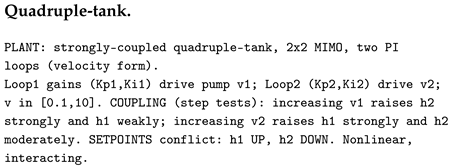
The parenthetical “velocity form” is historical prompt metadata and is inconsistent with the position-form implementation used to generate the saved labels (Appendix C). The text is retained here for auditability rather than silently rewriting the administered prompt. P0 replaces the first two lines with “strongly-coupled quadruple-tank, 2 × 2 MIMO, with two position-form PI loops” and adds the implemented saturation and integral-rollback description; the remaining plant information and all item texts are retained.
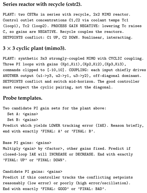
The code and saved filenames use the historical label stability for the third format. The administered question does not test control-theoretic stability; it asks whether IAE is above or below the median of the sampled pool. This paper therefore calls it tracking quality.
- Control-theory knowledge baseline (E1), representative items. All are forced-choice; the correct option is marked ✓.
- Increasing the proportional gain of a PI loop (other things equal) makes the closed-loop response: (A) faster but more oscillatory/prone to overshoot ✓; (B) slower and more sluggish.
- The main role of the integral term is to: (A) eliminate steady-state tracking offset ✓; (B) add high-frequency noise rejection.
- In a MIMO plant with strong cross-coupling, designing each decentralized loop independently tends to: (A) cause loop interaction that can degrade performance or destabilize ✓; (B) work perfectly because loops are independent.
- A controller that minimizes IAE while also penalizing control effort (TV) should avoid: (A) aggressive bang-bang actuation that saturates the actuator ✓; (B) any integral action at all.
- In this plant each input mainly drives a different output; tuning each loop on the diagonal pairing tends to: (A) perform poorly because the dominant coupling is off-diagonal ✓; (B) be optimal.
- Conflicting, switching set-points in a coupled MIMO plant generally require: (A) coordinated, possibly asymmetric tuning ✓; (B) identical aggressive gains on every loop.
The pooled E1 rate is on the tank and reactor and on mimo3; Llama-3.1-8B obtains on mimo3. Because E1 provides explicit qualitative options and does not require numerical performance comparison, it is a declarative reference rather than a matched control task.
- Gain sampling. Each gain is drawn log-uniformly over a wide range. The approximate ranges are and for the quadruple-tank; for the reactor (negative gains), and ; for the plant, and . Each plant’s pool of 320 gain sets spans two to three orders of magnitude per gain. All magnitude-rule percentages are conditional on these bounds and this log-uniform sampling distribution. P1 additionally constructs, for each plant and each of three seeds, one Latin-hypercube pool over the same log bounds and one independent log-uniform pool over the inner 80% of every log-gain interval.
Appendix B. Plant Equations and Simulation Protocol
- Quadruple-tank. The four states are liquid levels . With pump voltages , the deterministic model isThe tank model uses , , , , and . The horizon is 400 with 120 control intervals, initial levels , and pump bounds . At the midpoint, the set-point changes from to and the set-point from to . The decentralized pairing is crossed: loop 1 measures and drives , while loop 2 measures and drives .
- Recycle CSTR. For concentrations , temperatures , feed flow F, recycle L, and coolant temperatures , the model isParameters are , , , , , , , , , and . The flows are fixed at and . Coolant temperatures are bounded to , and the simulation uses 120 intervals over a horizon of 240. The initial state is ; set-points change from to at the midpoint.
- Cyclic plant. The discrete-time model isErrors are cyclically paired as and commands are clipped to . Over 120 steps, the set-point switches at the midpoint from to .
The tank and reactor equations and parameterizations follow the corresponding PC-Gym environments [39]; the cyclic model is defined in the project artifact. The saved pools and question files are the authoritative source for reported labels. A standalone SciPy replay of the first three saved controllers per plant reproduces IAE within approximately – for the two continuous plants and within for the cyclic plant. Small differences reflect the numerical integrator and gain rounding.
Appendix C. Implementation and Reproducibility
- Item counts and seeding. For each plant, a pool of 320 controllers is sampled. The quadruple-tank and plant each contribute 100 pairwise, 40 direction, 40 tracking-quality, and 16 E1 items per checkpoint (196 total). The reactor contributes 74, 40, 40, and 12 items, respectively (166 total); its pool contains no pair with an IAE ratio above 2, so no easy pairwise bin can be formed. Controller sampling and item construction use NumPy seed 20260611; primary simulations are deterministic with noise disabled and simulator seed 0. The perturbation sensitivity audit is described in Section 3.6. Direction and tracking-quality item builders approximately balance their two labels by construction.
P0 adds 180 corrected-metadata tank items per checkpoint (720 unique checkpoint–item outputs). P1 uses 2 sampling designs pool seeds plants pairs checkpoints, for 3600 fully parseable outputs. P2 uses 4 cells generation seeds proposals checkpoints, for 1280 proposal records. P3 uses 3 information conditions plants matched pairs checkpoints, for 1800 unique outputs. It additionally records 62 deterministic length-cap retries; the latest attempts yield 1792 parsed outputs. P4 uses 271 replay-stable pairs evidence conditions checkpoints, for 4336 unique outputs, plus 406 append-only length-cap retries. The metric audit adds 542 nominal controller replays. The perturbation audit uses 271 pairs controllers shared seeds, for 5420 additional simulations; it does not require new LLM inference.
- Simulation and cost. Each controller is evaluated by simulating the closed loop under the plant’s conflicting set-points and computing IAE. Prediction ground truth uses this cumulative tracking term. The distinct tuning ablation of Section 4.8 uses the full penalized J of Equation (2) with and total pump variation divided by 10. For the tank and reactor, IAE is evaluated by trapezoidal quadrature; the cyclic plant uses a discrete sum of post-update absolute errors times the step duration. Samples whose simulated cost is non-finite or exceeds a plant-specific cap ( for the quadruple-tank, for the reactor and the plant) are discarded before items are built.
- PI implementation. For the tank and reactor, each loop uses position-form PI with a constant actuator bias:If saturation occurs and , the most recent integral increment is rolled back. Biases are 5 for tank pumps and 350 for reactor coolant temperatures. The cyclic plant uses the same position-form update without rollback and with zero bias. The historical tank description incorrectly called this velocity-form PI; P0 corrects the description while retaining the saved questions and labels.
- Models and inference. The four primary checkpoints (Qwen3-14B, Qwen2.5-14B, Qwen2.5-7B, Llama-3.1-8B) are served in bfloat16 on a single 48 GB GPU; the scale test (Section 4.10) runs Qwen2.5-32B in 4-bit nf4 quantization with a bfloat16 compute dtype so that it fits on one card. Prediction-probe decoding is greedy (temperature 0). Each checkpoint is instructed to end with an explicit decision token, which a fixed parser extracts (FINAL: A/B, UP/DOWN, or GOOD/BAD). Raw accuracy scores unparsed responses as incorrect; coverage and parsed-only accuracy are reported separately in Table 3. The reasoning check uses Qwen3 thinking mode or an explicit step-by-step instruction, temperature , and top-. P2 uses temperature , top-, ten generation seeds per cell, and exactly eight proposals in every cell. Of 1280 proposal records, 1254 contain a valid parsed controller and finite J; every checkpoint–cell–seed group has at least one valid proposal, and best J is computed over the valid proposals. P3 uses greedy decoding and a two-sentence output constraint with a 192-token cap. The 62 initially uninterpretable outputs are regenerated with the same prompt and greedy decoding at a 512-token cap, and only the latest attempt is scored. Final Q/E/T parse coverage is 598/600, 600/600, and 594/600. P4 also uses greedy decoding, initially at 128 tokens. It regenerates the 406 initially unparsed Llama outputs from identical prompts at a 384-token cap and scores only the latest attempt. The append-only logs contain 4742 records for 4336 unique checkpoint–item–condition keys; 4306 final outputs parse, and condition coverage is 1079/1084 (Q), 1071/1084 (T), 1073/1084 (X), and 1083/1084 (S). Across the 1084 final P4 records per checkpoint, median logged request times are 0.54 s for Qwen3-14B, 0.47 s for Qwen2.5-14B, 0.18 s for Qwen2.5-7B, and 0.64 s for Llama-3.1-8B; the corresponding interquartile ranges are 0.38–0.60, 0.32–0.58, 0.12–0.24, and 0.45–0.71 s. These deployment-specific wall-clock measurements include serving overhead and do not establish real-time suitability under different hardware, batching, or concurrency.
Appendix D. Checkpoint-Level Gain and Prompt-Choice Summaries
Table A1 reports the numerical values underlying the P1 raw and normalized agreement panels in Figure 7. Each mean and sample SD uses three independently sampled controller pools, with 50 label-balanced items per checkpoint and pool. The normalization is an analysis of the same choices, not a rescaled-gain prompting experiment.
Table A1.
P1 checkpoint-level agreement with the lower-magnitude rule: mean ± sample SD across three pool seeds (%). Each checkpoint–plant–design combination contains 150 parsed choices.
Table A2 summarizes the latest saved P3 responses on the same 150 items per condition and checkpoint, with 75 A and 75 B ground-truth labels. Under T, A-choice rates among parsed responses are 39.3%, 36.7%, 88.0%, and 96.5% for Qwen3-14B, Qwen2.5-14B, Qwen2.5-7B, and Llama-3.1-8B, respectively. The corresponding Q rates are 48.0%, 60.7%, 78.0%, and 77.0%. These unequal frequencies are descriptive option preferences. Table placement and candidate order were fixed, so their causal contribution and any context-window decay remain unmeasured. Character counts refer to the stored system and user text, excluding checkpoint-specific chat-template tokens.
Table A2.
P3 option frequencies for the qualitative (Q) and trajectory (T) conditions. Counts sum to 150 in each condition; unparsed responses remain separate from A and B.
References
- Tohma, K.; Okur, H.I.; Gürsoy-Demir, H.; Aydın, M.N.; Yeroğlu, C. SmartControl: Interactive PID controller design powered by LLM agents and control system expertise. SoftwareX 2025, 31, 102194. [Google Scholar] [CrossRef] [Scilit]
- Ares-Milian, M.J.; Provan, G.; Quinones-Grueiro, M. Automating control system design: Using language models for expert knowledge in decentralized controller auto-tuning. In Proceedings of the 36th International Conference on Principles of Diagnosis and Resilient Systems (DX 2025); Open Access Series in Informatics (OASIcs); Schloss Dagstuhl–Leibniz- Zentrum für Informatik: Dagstuhl, Germany, 2025; Volume 136, pp. 10:1–10:20. [Google Scholar] [CrossRef]
- Khoo, T.L.; Lee, T.S.; Bee, S.-T.; Ma, C.; Zhang, Y.-Y. A comparative review of large language models in engineering with emphasis on chemical engineering applications. Processes 2025, 13, 2680. [Google Scholar] [CrossRef] [Scilit]
- Jiang, X.; Xie, H.; Wang, J.; Yang, Z.; Zhou, Y.; Yao, L.; Zhu, Z. Agentic AI for safety-aware process monitoring and fault diagnosis: A review. Processes 2026, 14, 2112. [Google Scholar] [CrossRef] [Scilit]
- Du, W.; Yang, S. The potential and challenges of large language model agent systems in chemical process simulation: From automated modeling to intelligent design. Front. Chem. Sci. Eng. 2025, 19, 99. [Google Scholar] [CrossRef] [Scilit]
- Chen, Y.; Luo, X.; Zhou, Y.; Peng, Q.; Yuan, Y.; Chen, K.; Liu, Y. Virtual-document-augmented retrieval-augmented generation for power-domain knowledge-base question answering with noise-enhanced robustness. Processes 2026, 14, 670. [Google Scholar] [CrossRef] [Scilit]
- Kiangala, K.S.; Wang, Z. Towards sustainable Industry 5.0: An LLM-based co-pilot for energy-efficient factory scheduling. Processes 2026, 14, 709. [Google Scholar] [CrossRef] [Scilit]
- Papacharalampopoulos, A.; Karagianni, O.M.; Stavropoulos, P. Cognitive supervisory control with LLM reasoning agent for fault-tolerant process systems: A digital twin perspective. Processes 2026, 14, 2298. [Google Scholar] [CrossRef] [Scilit]
- Galitsky, B.; Rybalov, A. Neuro-symbolic verification for preventing LLM hallucinations in process control. Processes 2026, 14, 322. [Google Scholar] [CrossRef] [Scilit]
- González-Potes, A.; Martínez-Castro, D.; Paredes, C.M.; Ochoa-Brust, A.; Mena, L.J.; Martínez-Peláez, R.; Félix, V.G.; Félix-Cuadras, R.A. Hybrid AI and LLM-enabled agent-based real-time decision support architecture for industrial batch processes: A clean-in-place case study. AI 2026, 7, 51. [Google Scholar] [CrossRef] [Scilit]
- Wang, L.; Ouyang, L.; Weng, H.; Chen, X.; Wang, A.; Zhang, K. Intelligent disassembly system for PCB components integrating multimodal large language model and multi-agent framework. Processes 2026, 14, 227. [Google Scholar] [CrossRef] [Scilit]
- Wu, J.; Chen, Y.; Min, Q.; Chen, M.; Zhao, J.; Ye, M. Domain-adaptive multimodal large language models for photovoltaic fault diagnosis via dynamic LoRA routing. Processes 2026, 14, 653. [Google Scholar] [CrossRef] [Scilit]
- Huang, K.; Chen, Q. Motor fault diagnosis and predictive maintenance based on a fine-tuned Qwen2.5-7B model. Processes 2025, 13, 2051. [Google Scholar] [CrossRef] [Scilit]
- Nosrati, K.; Tepljakov, A.; Belikov, J.; Petlenkov, E. When control meets large language models: From words to dynamics. Eng. Appl. Artif. Intell. 2026, 178, 115119. [Google Scholar] [CrossRef] [Scilit]
- Wen, H.; Roberts, J.; Zaidi, A.; McLeod, A. An experiment of using a large language model to control a water tank system. Comput. Chem. Eng. 2026, 211, 109656. [Google Scholar] [CrossRef] [Scilit]
- Schall, D. Safe integration of large language models into industrial process control: A multi-agent architecture with P&ID-grounded validation. Auton. Intell. Syst. 2026, 6, 14. [Google Scholar] [CrossRef] [Scilit]
- Kevian, D.; Syed, U.; Guo, X.; Havens, A.; Dullerud, G.; Seiler, P.; Qin, L.; Hu, B. Capabilities of large language models in control engineering: A benchmark study on GPT-4, Claude 3 Opus, and Gemini 1.0 Ultra. arXiv 2024, arXiv:2404.03647. [Google Scholar] [CrossRef] [Scilit]
- Mahowald, K.; Ivanova, A.A.; Blank, I.A.; Kanwisher, N.; Tenenbaum, J.B.; Fedorenko, E. Dissociating language and thought in large language models. Trends Cogn. Sci. 2024, 28, 517–540. [Google Scholar] [CrossRef] [Scilit] [PubMed]
- Valmeekam, K.; Marquez, M.; Olmo, A.; Sreedharan, S.; Kambhampati, S. PlanBench: An extensible benchmark for evaluating large language models on planning and reasoning about change. In Advances in Neural Information Processing Systems; Curran Associates, Inc.: Red Hook, NY, USA, 2023; Volume 36, pp. 38975–38987. [Google Scholar]
- Bender, E.M.; Gebru, T.; McMillan-Major, A.; Shmitchell, S. On the dangers of stochastic parrots: Can language models be too big? In Proceedings of the 2021 ACM Conference on Fairness, Accountability, and Transparency, Virtual, 3–10 March 2021; ACM: New York, NY, USA, 2021; pp. 610–623. [Google Scholar] [CrossRef] [Scilit]
- Chen, Z.; Chen, W.; Smiley, C.; Shah, S.; Borova, I.; Langdon, D.; Moussa, R.; Beane, M.; Huang, T.-H.; Routledge, B.; et al. FinQA: A dataset of numerical reasoning over financial data. In Proceedings of the 2021 Conference on Empirical Methods in Natural Language Processing, Punta Cana, Dominican Republic, 7–11 November 2021; pp. 3697–3711. [Google Scholar] [CrossRef] [Scilit]
- Zhu, F.; Lei, W.; Huang, Y.; Wang, C.; Zhang, S.; Lv, J.; Feng, F.; Chua, T.-S. TAT-QA: A question answering benchmark on a hybrid of tabular and textual content in finance. In Proceedings of the 59th Annual Meeting of the Association for Computational Linguistics and the 11th International Joint Conference on Natural Language Processing, Online, 1–6 August 2021; pp. 3277–3287. [Google Scholar]
- Sui, Y.; Zhou, M.; Zhou, M.; Han, S.; Zhang, D. Table meets LLM: Can large language models understand structured table data? A benchmark and empirical study. In Proceedings of the 17th ACM International Conference on Web Search and Data Mining, Mérida, Mexico, 4–8 March 2024; pp. 645–654. [Google Scholar]
- Wang, Z.; Zhang, H.; Li, C.-L.; Eisenschlos, J.M.; Perot, V.; Wang, Z.; Miculicich, L.; Fujii, Y.; Shang, J.; Lee, C.-Y.; et al. Chain-of-Table: Evolving tables in the reasoning chain for table understanding. In Proceedings of the 12th International Conference on Learning Representations, Vienna, Austria, 7–11 May 2024. [Google Scholar]
- Li, H.; Chen, X.; Xu, Z.; Li, D.; Hu, N.; Teng, F.; Li, Y.; Qiu, L.; Zhang, C.J.; Li, Q.; et al. Exposing numeracy gaps: A benchmark to evaluate fundamental numerical abilities in large language models. In Proceedings of the Findings of the Association for Computational Linguistics: ACL 2025, Vienna, Austria, 27 July–1 August 2025; pp. 20004–20026. [Google Scholar] [CrossRef] [Scilit]
- Li, L.; Tian, J.; Chen, H.; Ye, W.; Ye, C.; Wang, H.; Wang, N.; Fu, X.; Chen, G.; Zhao, J. LongTableBench: Benchmarking long-context table reasoning across real-world formats and domains. In Proceedings of the Findings of the Association for Computational Linguistics: EMNLP 2025, Suzhou, China, 4–9 November 2025; pp. 11927–11965. [Google Scholar]
- Gao, L.; Madaan, A.; Zhou, S.; Alon, U.; Liu, P.; Yang, Y.; Callan, J.; Neubig, G. PAL: Program-aided language models. In Proceedings of the 40th International Conference on Machine Learning, Honolulu, HI, USA, 23–29 July 2023; Volume 202, pp. 10764–10799. [Google Scholar]
- Chen, W.; Ma, X.; Wang, X.; Cohen, W.W. Program of thoughts prompting: Disentangling computation from reasoning for numerical reasoning tasks. Trans. Mach. Learn. Res. 2023. Available online: https://openreview.net/forum?id=YfZ4ZPt8zd (accessed on 27 August 2026).
- Schick, T.; Dwivedi-Yu, J.; Dessì, R.; Raileanu, R.; Lomeli, M.; Hambro, E.; Zettlemoyer, L.; Cancedda, N.; Scialom, T. Toolformer: Language models can teach themselves to use tools. In Proceedings of the Advances in Neural Information Processing Systems, New Orleans, LA, USA, 10–16 December 2023; Volume 36, pp. 68539–68551. [Google Scholar] [CrossRef] [Scilit]
- Åström, K.J.; Hägglund, T. Advanced PID Control; ISA: Research Triangle Park, NC, USA, 2006. [Google Scholar]
- Skogestad, S. Simple analytic rules for model reduction and PID controller tuning. J. Process Control 2003, 13, 291–309. [Google Scholar] [CrossRef] [Scilit]
- Garcia, C.E.; Morari, M. Internal model control. A unifying review and some new results. Ind. Eng. Chem. Process Des. Dev. 1982, 21, 308–323. [Google Scholar] [CrossRef] [Scilit]
- Bristol, E. On a new measure of interaction for multivariable process control. IEEE Trans. Autom. Control 1966, 11, 133–134. [Google Scholar] [CrossRef] [Scilit]
- Skogestad, S.; Postlethwaite, I. Multivariable Feedback Control: Analysis and Design, 2nd ed.; Wiley: Chichester, UK, 2005. [Google Scholar]
- Hjalmarsson, H. Iterative feedback tuning—An overview. Int. J. Adapt. Control Signal Process. 2002, 16, 373–395. [Google Scholar] [CrossRef] [Scilit]
- Hou, Z.; Wang, Z. From model-based control to data-driven control: Survey, classification and perspective. Inf. Sci. 2013, 235, 3–35. [Google Scholar] [CrossRef] [Scilit]
- Bujgoi, G.; Sendrescu, D. Tuning of PID controllers using reinforcement learning for nonlinear system control. Processes 2025, 13, 735. [Google Scholar] [CrossRef] [Scilit]
- Daskin, M. Optimization of weighted geometrical center method for PI and PI–PD controllers. Processes 2025, 13, 749. [Google Scholar] [CrossRef] [Scilit]
- Bloor, M.; Torraca, J.; Sandoval, I.O.; Ahmed, A.; White, M.; Mercangöz, M.; Tsay, C.; Del Rio Chanona, E.A.; Mowbray, M. PC-Gym: Benchmark environments for process control problems. Comput. Chem. Eng. 2026, 204, 109363. [Google Scholar] [CrossRef] [Scilit]
- Moerland, T.M.; Broekens, J.; Plaat, A.; Jonker, C.M. Model-based reinforcement learning: A survey. Found. Trends Mach. Learn. 2023, 16, 1–118. [Google Scholar] [CrossRef] [Scilit]
- Ha, D.; Schmidhuber, J. Recurrent world models facilitate policy evolution. In Proceedings of the Advances in Neural Information Processing Systems, Montreal, QC, Canada, 2–8 December 2018; Volume 31, pp. 2450–2462. Available online: https://proceedings.neurips.cc/paper/2018/hash/2de5d16682c3c35007e4e92982f1a2ba-Abstract.html (accessed on 27 August 2026).
- Johansson, K.H. The quadruple-tank process: A multivariable laboratory process with an adjustable zero. IEEE Trans. Control Syst. Technol. 2000, 8, 456–465. [Google Scholar] [CrossRef] [Scilit]
- Yang, A.; Li, A.; Yang, B.; Zhang, B.; Hui, B.; Zheng, B.; Yu, B.; Gao, C.; Huang, C.; Lv, C.; et al. Qwen3 technical report. arXiv 2025, arXiv:2505.09388. [Google Scholar]
- Qwen Team. Qwen2.5 technical report. arXiv 2024, arXiv:2412.15115. [Google Scholar] [CrossRef] [Scilit]
- Grattafiori, A.; Dubey, A.; Jauhri, A.; Pandey, A.; Kadian, A.; Al-Dahle, A.; Letman, A.; Mathur, A.; Schelten, A.; Vaughan, A.; et al. The Llama 3 herd of models. arXiv 2024, arXiv:2407.21783. [Google Scholar] [CrossRef] [Scilit]
- Wei, J.; Wang, X.; Schuurmans, D.; Bosma, M.; Ichter, B.; Xia, F.; Chi, E.; Le, Q.; Zhou, D. Chain-of-thought prompting elicits reasoning in large language models. In Proceedings of the Advances in Neural Information Processing Systems, New Orleans, LA, USA, and Online, 28 November–9 December 2022; Volume 35, pp. 24824–24837. [Google Scholar] [CrossRef] [Scilit]
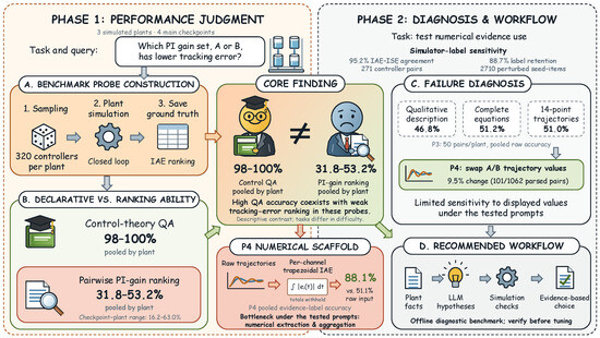
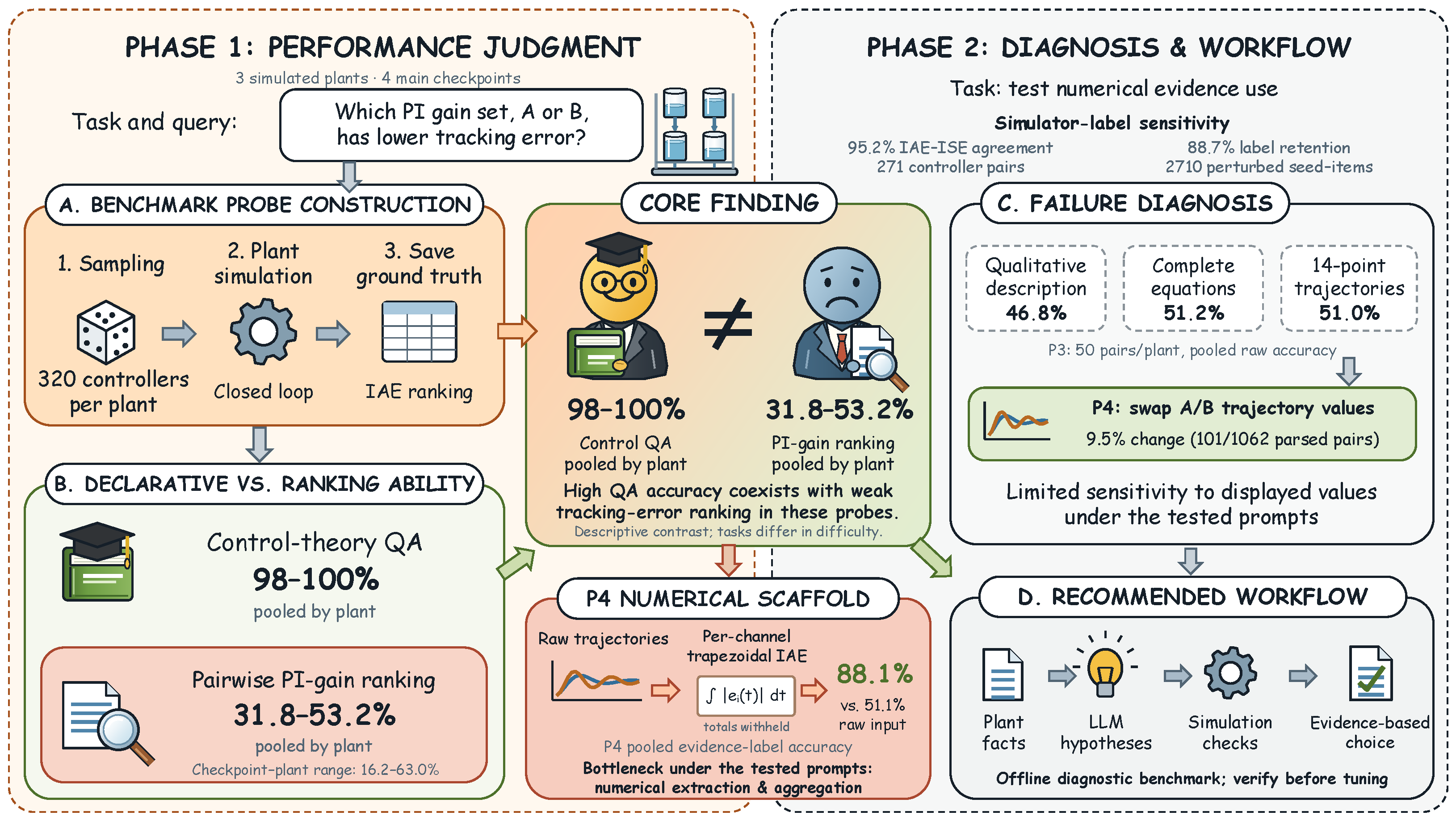
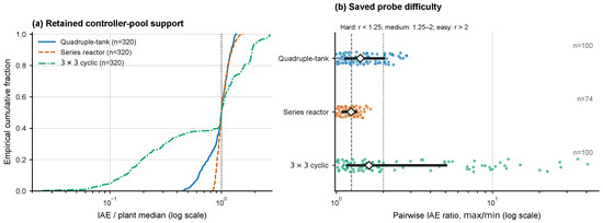
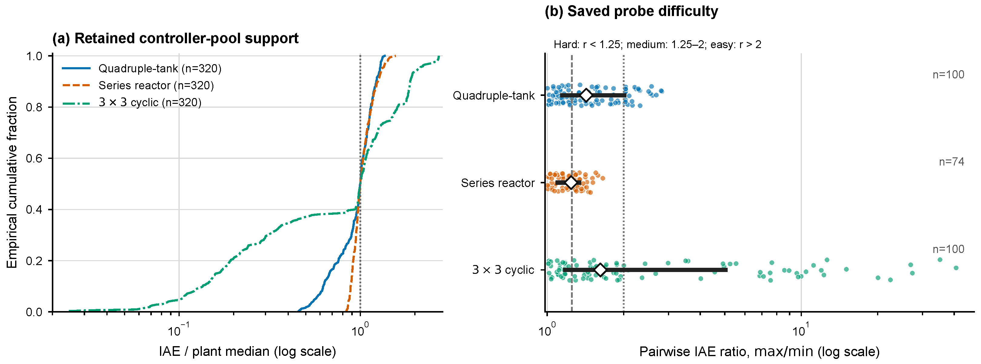
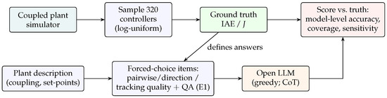
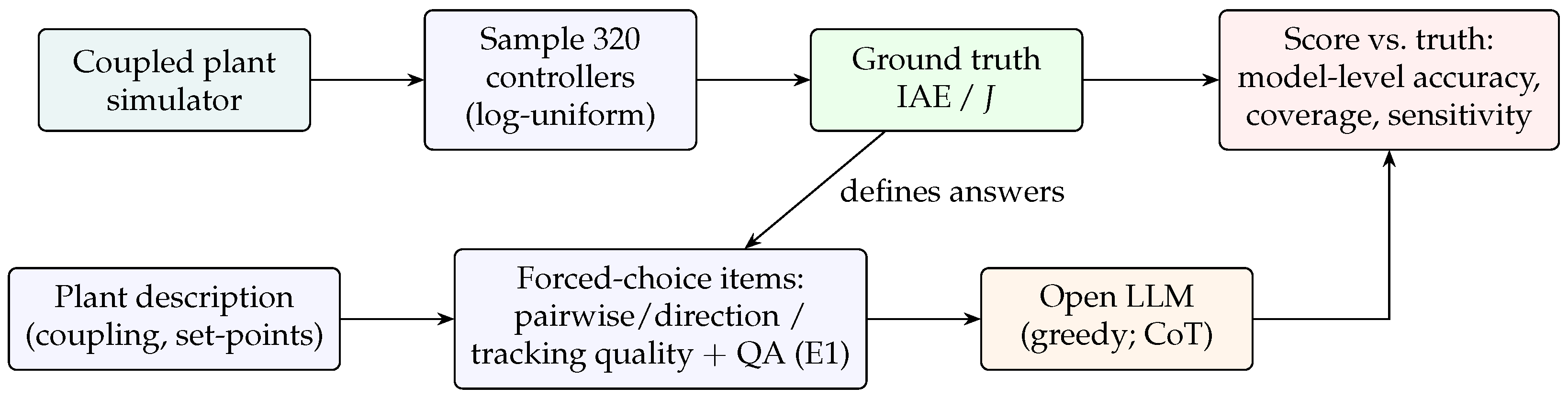
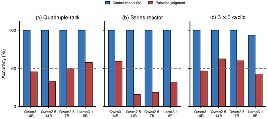
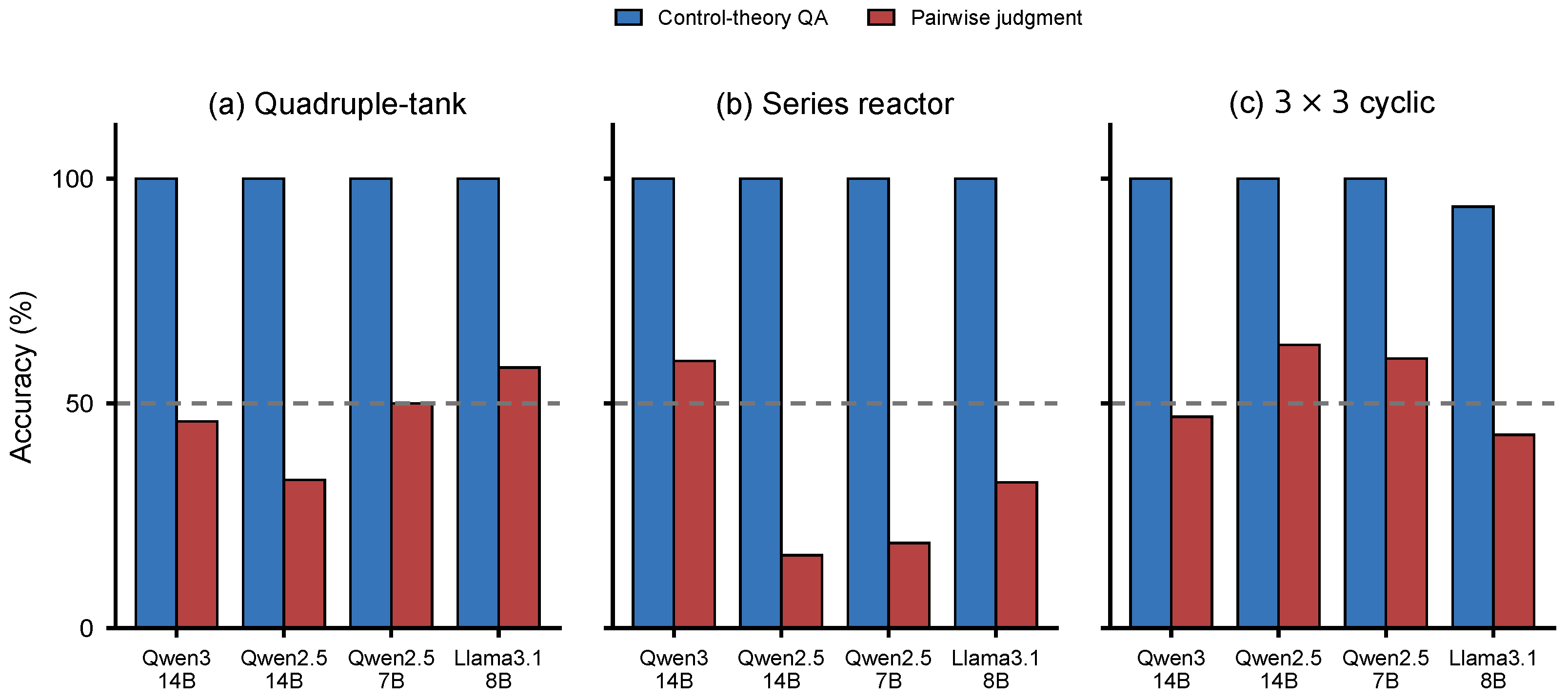
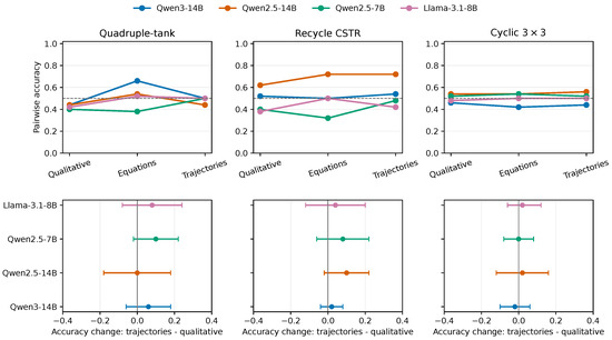
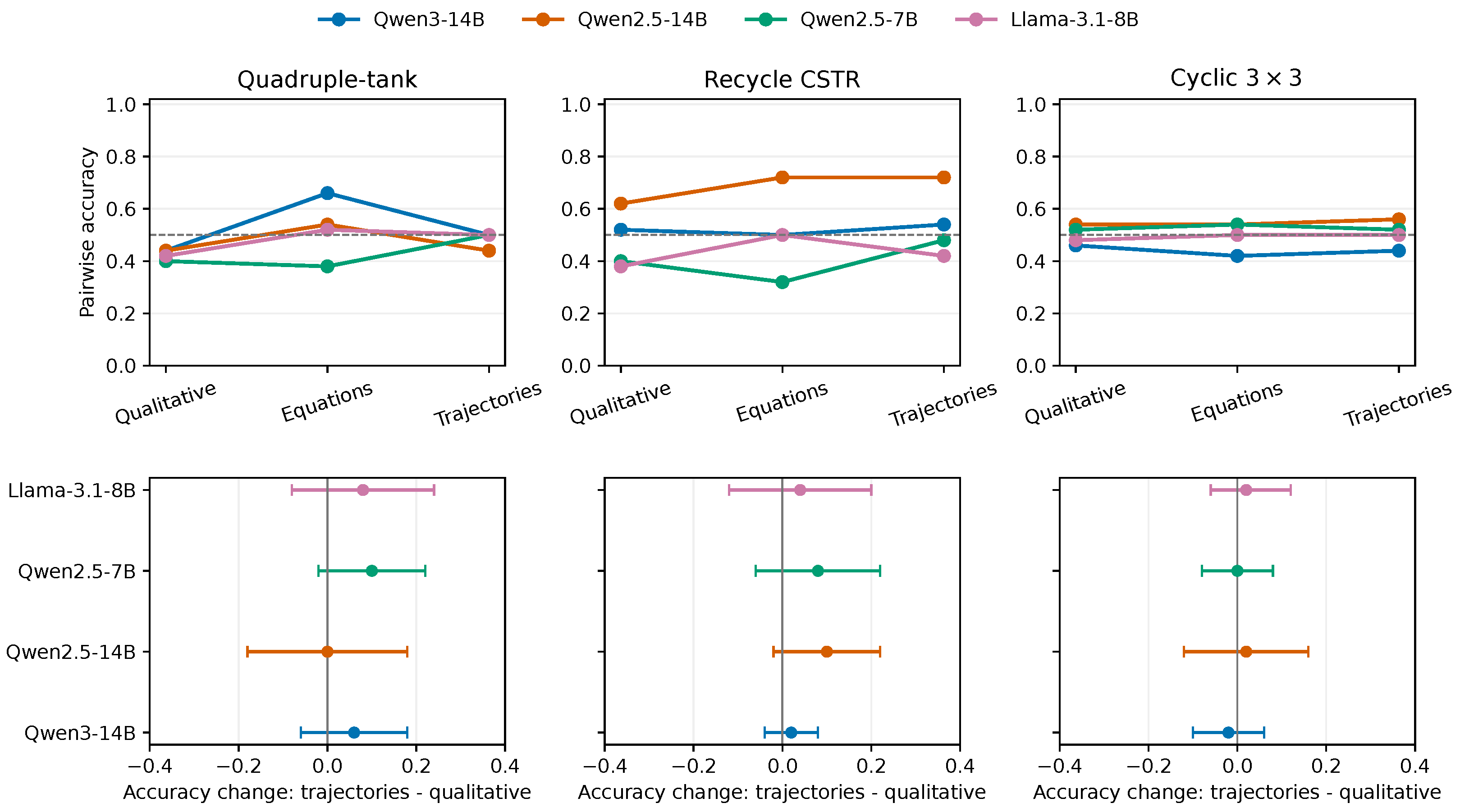
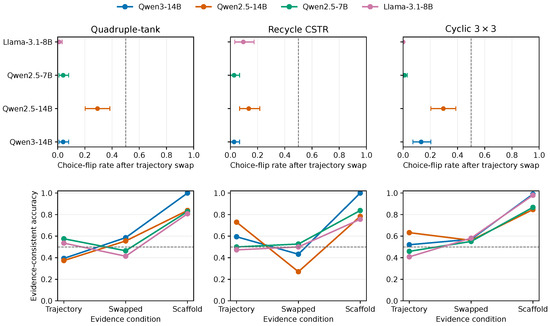
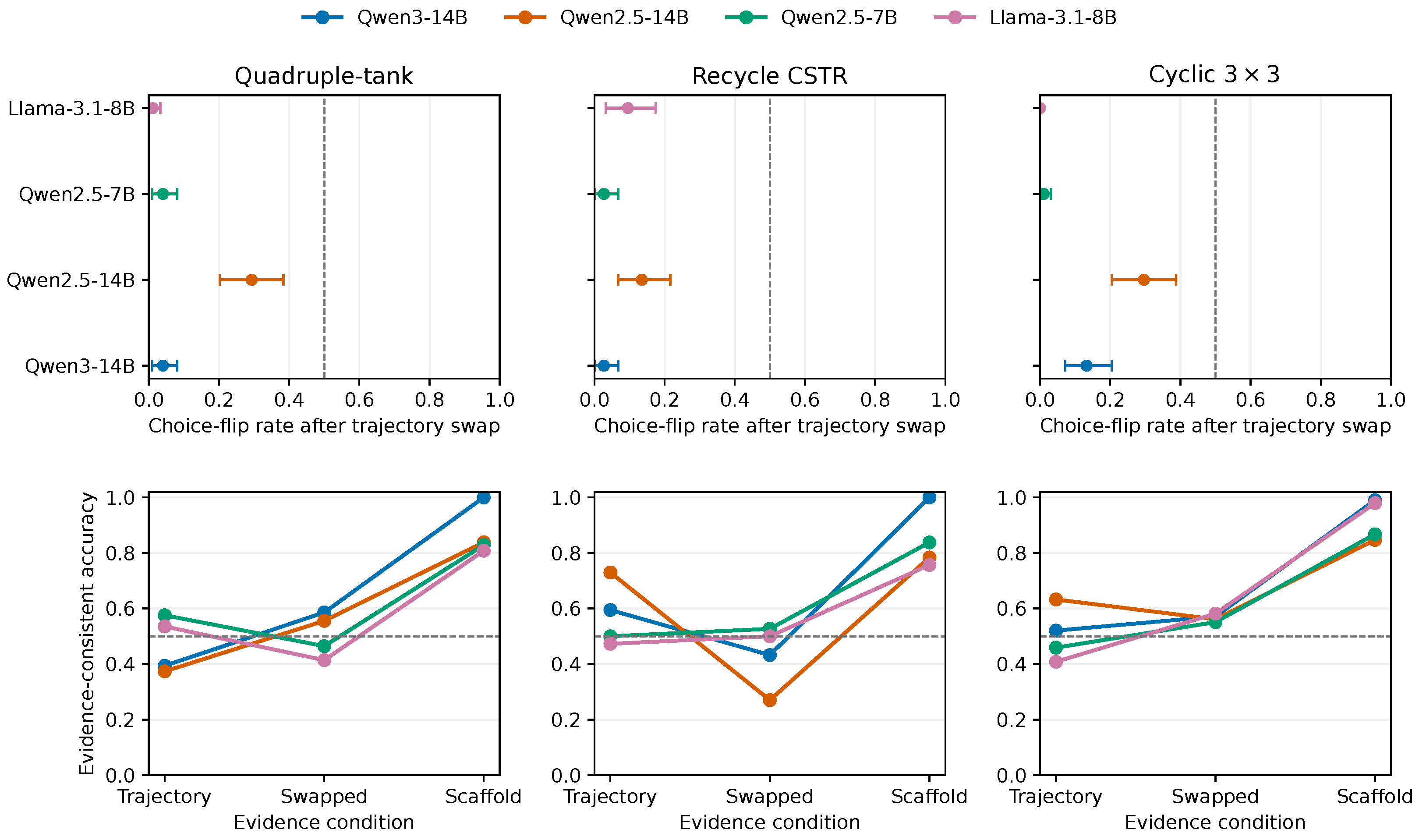
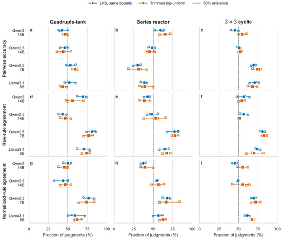
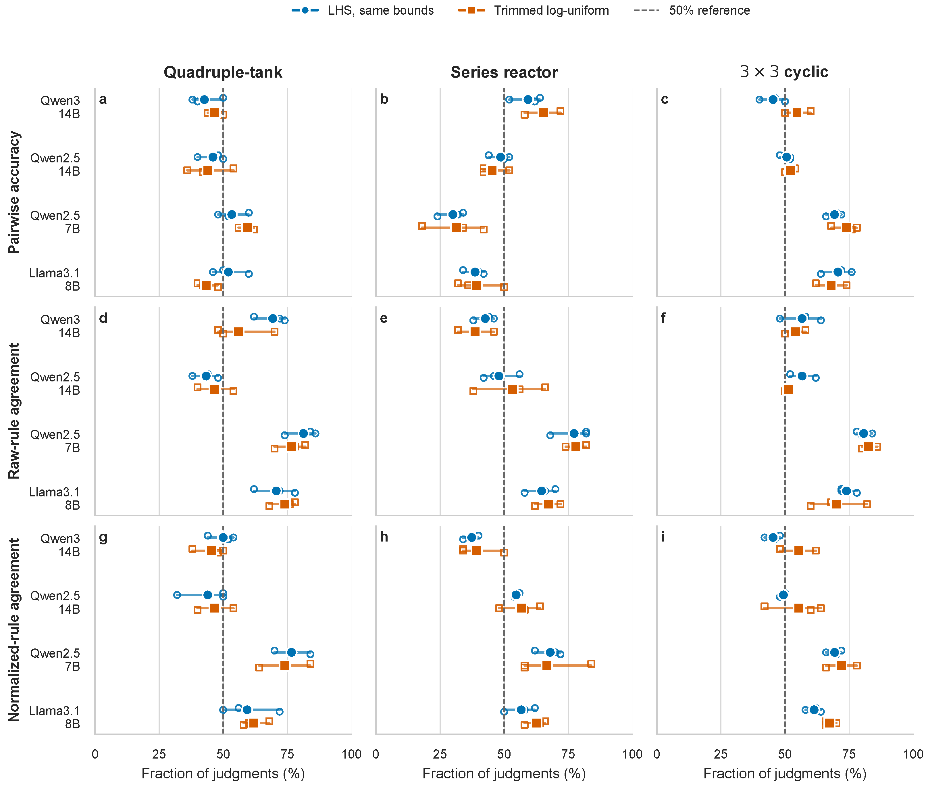
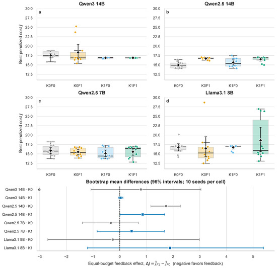
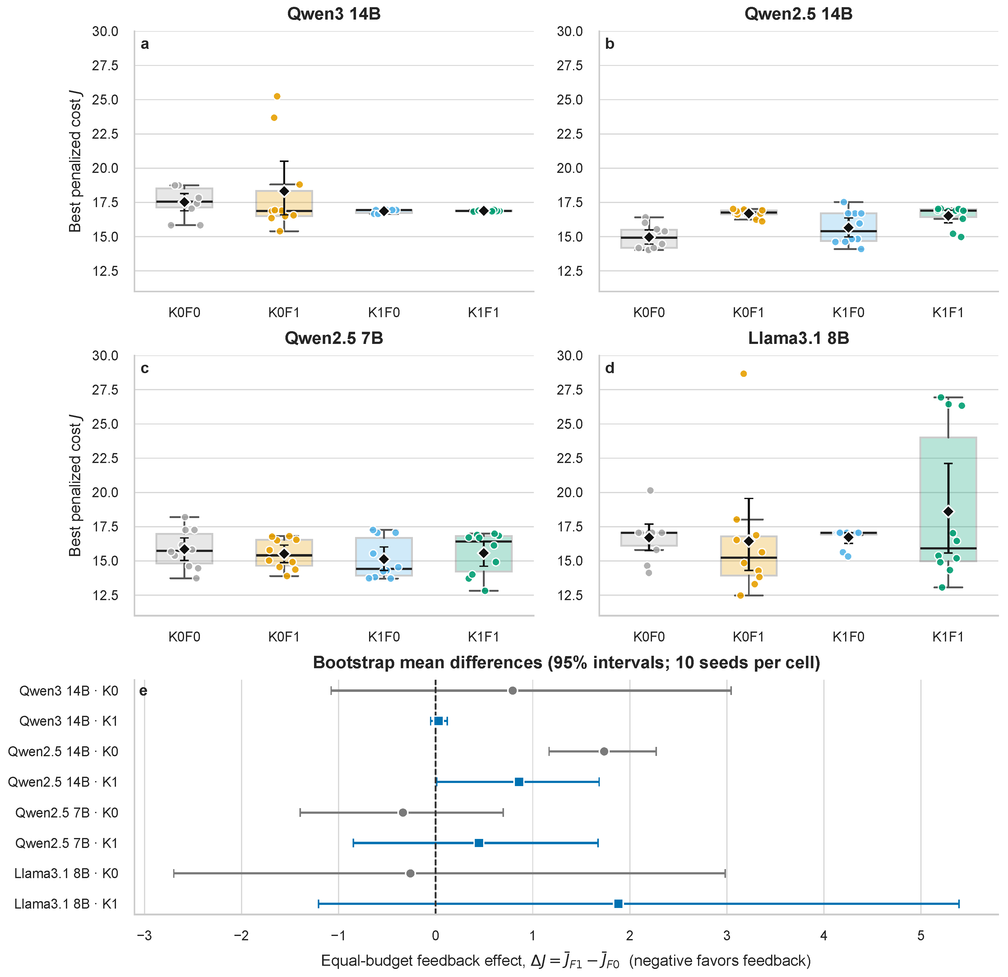
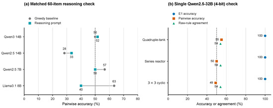
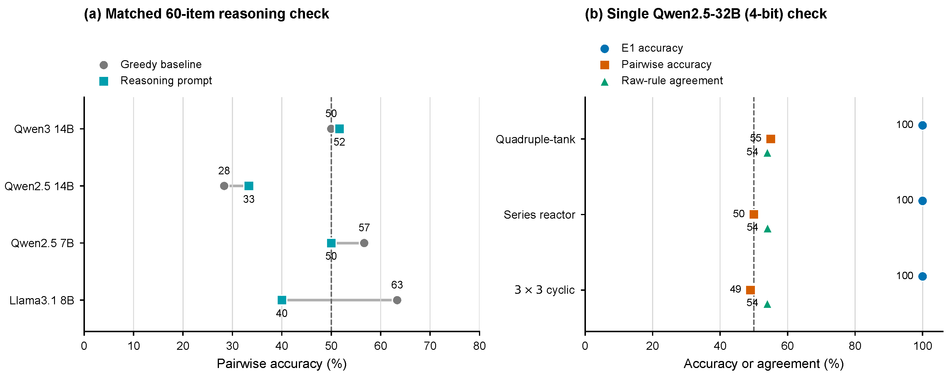

Disclaimer/Publisher’s Note: The statements, opinions and data contained in all publications are solely those of the individual author(s) and contributor(s) and not of MDPI and/or the editor(s). MDPI and/or the editor(s) disclaim responsibility for any injury to people or property resulting from any ideas, methods, instructions or products referred to in the content. |
© 2026 by the authors. Licensee MDPI, Basel, Switzerland. This article is an open access article distributed under the terms and conditions of the Creative Commons Attribution (CC BY) license.