


Abstract
Due to the rising share of renewable energy sources within distribution systems, there is a need for planning methods that can accommodate wind uncertainty. This paper introduces a holistic bi-level optimization approach for the optimal planning of wind-based distributed generation (WBDG) and battery energy storage system (BESS). At the higher level, the optimal location and size of WBDG and BESS are selected based on minimizing power loss, improving voltage stability, and minimizing the cost of electricity production. Meanwhile, at the lower level, the BESS charging–discharging operations and power transmission between different wind situations are scheduled. Wind uncertainty is considered in the model by applying the Weibull probability density function in combination with the Two-Point Estimation Method (2m-PEM). The resulting complicated bi-level optimization issue is addressed by creating a new Improved Cheetah Optimizer (ICO) that incorporates four enhancements to the Cheetah Optimizer (CO) to improve its explorative and exploitative capabilities. Simulations conducted on the IEEE 33-bus system show the superiority of the proposed method compared to other methods. The ICO outperforms particle swarm optimization (PSO), genetic algorithm (GA), and the basic CO by achieving up to 69.07% daily energy savings, raising the lowest bus voltage from 0.9440 per unit to 0.9610 per unit, and providing an expected operating cost of $5449.92.
1. Introduction
The rapid depletion of traditional energy sources and their environmental repercussions have led to a shift towards sustainable energy. Traditional sources of energy, such as fossil fuel plants, are not only exhaustible but also a cause of greenhouse gases that led to the creation of the Kyoto agreement and COP26 [1,2]. As a result, several countries have pledged tangible targets for renewable deployment, where countries like India are aiming for 40% renewables by 2030, along with major solar initiatives [3,4]. It is clear from these pledges that there is a need for developing methods of planning that would allow higher penetration levels of renewable-based distributed generation (RG) [5,6,7]. Wind energy has proven to be one of the most viable renewable sources of energy as far as technological advancement and generation cost are concerned. Nevertheless, the unpredictability of wind energy poses certain difficulties during implementation. The widespread use of Wind-Based Distributed Generation (WBDG) could result in voltage instability, power loss, and unreliability [8]. Intermittent problems are also very common in photovoltaic-based distributed generation systems, where fluctuations in solar radiation lead to an imbalance between the amount of power generated locally and the power consumed, resulting in poor voltage management and inefficient operation [9,10,11]. These issues highlight the importance of intelligent planning approaches that can address the variability of renewable energy sources.
The conventional method used for handling the intermittent nature of renewable energy sources is incorporating battery energy storage systems (BESS). BESS can store extra energy when production is high and release stored energy when production is low [9,12]. In PV-dominated microgrids, it is observed that coordination between PV and BESS operations has proven to be effective in improving voltage profiles, minimizing losses, and achieving efficient use of distributed energy sources [9,10]. Whereas these principles have been widely adopted by PV systems, their implementation for wind-based systems needs special focus on time-specific features of wind fluctuations.
Planning of systems based on the WBDG and BESS is a complex multiple-objective optimization problem since it involves interconnected investment and operational decisions. Investment and operational decisions should observe nonlinear power flow equations and uncertainties related to demands and the availability of renewables. Bi-level optimization models have demonstrated great efficiency when applied to such optimization problems because they implicitly reflect the correlation between long-term decision-making and operational decisions. For microgrid systems based on photovoltaic generators, bi-level optimization techniques have already been applied to solve energy losses minimization and voltage stabilization problems while accounting for load and renewable uncertainties [9,10,11]. The efficiency of those methods can be a promising approach to applying bi-level optimization techniques to wind systems.
In line with the design of planning strategies, a wealth of literature has centered around the formulation of DG placement and optimization strategies. Many heuristic and meta-heuristic approaches have been used for solving DG planning under uncertain conditions, such as the Honey Badger Optimization algorithm (HBO), which has shown excellent performance in managing both discrete and continuous decision variables while dealing with multi-objective issues [9,12,13]. Other novel optimization strategies have emerged, such as Artificial Ecosystem-Based Optimization using Opposition-Based Learning (AEO-OBL), which shows faster convergence compared to algorithms like HHO and HGSO [14]. The Cheetah Optimizer (CO), introduced in [15], has shown promise for complex nonlinear power system problems due to its balanced exploration-exploitation mechanisms [13,15].
A precise representation of the uncertainty associated with wind energy is vital for efficient WBDG-BESS design. Variability in wind speed depends on the terrain and weather, which affects the amount of power generated by wind turbines according to their non-linear power curves [16]. The Weibull probability distribution is widely adopted for modeling wind speed patterns due to its robustness and accuracy [17,18,19], with studies indicating that the empirical method provides the most reliable parameter estimation among common techniques [20]. In order to propagate the uncertainty in wind speed without a high computation cost, the 2m-PEM technique provides an efficient approach compared to the Monte Carlo simulation [9,12,21]. In PV-based DG planning, 2m-PEM has been effectively employed to represent solar radiation and load uncertainties while maintaining computational tractability [9,22].
In spite of the existing efforts made in the area of DG planning, uncertainty modeling, and optimization, there is still a need for developing a holistic approach that would address the needs of WBDG and BESS in particular. Such an approach would require a modeling of wind uncertainty with the help of sophisticated probabilistic tools; a bi-level approach to solving the problem in terms of optimal DG placement, sizing, and operation scheduling; as well as the use of a highly effective metaheuristic algorithm for exploring the resultant solution space. Inspired by bi-level optimization approaches developed for PV systems [9,11] and the potential of advanced metaheuristics [15,17], this paper proposes such an integrated solution.
The specific novelties of this work are threefold. First, this study presents the first application of the Cheetah Optimizer (and its improved variant) to the bi-level planning of wind-based distributed generation and battery energy storage under wind uncertainty—a problem structure coupling investment decisions, operational scheduling, and uncertainty propagation that has not previously been solved with CO or its derivatives. Second, the proposed ICO introduces four targeted enhancement mechanisms (leader-guided search, rank-based step adaptation, distance-weighted interaction, and adaptive exploration-exploitation balance) that are specifically designed to address the mixed-integer, non-convex, and multi-modal characteristics of DG planning problems, not merely generic modifications. Third, the integration of the Two-Point Estimation Method (2m-PEM) with a bi-level DG/BESS planning framework provides a computationally efficient alternative to Monte Carlo simulation for wind uncertainty handling, which is novel in this context. This work extends the bi-level and uncertainty-aware concepts successfully applied to PV-DG and BESS [9,10,11] to wind resources, providing a comprehensive planning approach for future distribution networks with high renewable penetration.
The rest of this paper will proceed as follows. Section 2 formulates the bi-level planning problem, including the upper-level investment model, lower-level operational model, BESS constraints, network constraints, inter-level coupling, and wind uncertainty characterization via the Two-Point Estimation Method. Section 3 presents the Improved Cheetah Optimizer, detailing the four enhancement mechanisms and the integration with the bi-level framework. The numerical analysis and comparisons in Section 4 will be conducted using the IEEE 33-bus test system. The statistical performance evaluation and optimization configurations will also be presented. Section 5 concludes the paper with key findings and directions for future research.
2. Problem Formulation
This section presents the proposed optimization framework for the integrated planning and operation of wind-based distributed generation (WBDG) and battery energy storage systems (BESS) in radial distribution networks. The problem inherently involves two distinct but strongly interdependent decision-making horizons: long-term investment decisions regarding the location and capacity of infrastructure assets, and short-term operational scheduling that determines how those assets are utilized under time-varying and uncertain conditions. The physical installation location and size impose fundamental limitations on the behavior of the system. The feasibility of operations and the cost of operations eventually define whether an investment is economically feasible or not. In order to adequately model the hierarchical interaction between these two aspects, we consider a bi-level optimization model. In the higher level of this model, the planning decisions for optimal installation of WBDGs and BESS are made. In the lower level of this model, the optimal operation schedule within a 24 h horizon is determined. The upper level is solved using the Improved Cheetah Optimizer (ICO) due to its strong exploration capability for mixed discrete-continuous problems. For each candidate planning solution generated by ICO, the lower level performs operational scheduling and AC power flow evaluation to compute the operational cost and verify system constraints.
2.1. Bi-Level Optimization Framework
The suggested framework disaggregates the joint planning-operation decision-making process into a hierarchy of two levels, each associated with its own specific time horizon and decision types. The upper level constitutes the planning level and determines the optimal number, location, and capacities of WBDG and BESS units by minimizing a total cost function that aggregates investment expenditures, maintenance costs, and the expected operational costs returned from the lower level. The lower level constitutes the operational level and determines the optimal hourly operation of BESS units while evaluating network performance through full AC power flow analysis. The lower level functions as a feasibility and cost evaluation layer, feeding the operational cost back to the upper level as a component of the overall objective function. This bidirectional interaction guarantees the feasibility of the obtained planning decisions as well as their optimality from an economic perspective.
2.2. Upper-Level Optimization: Planning Model
The upper-level problem determines the optimal placement and sizing of WBDG and BESS units within the distribution network. The decision variables at this level comprise the installation buses for WBDG units, the installed capacities of WBDG units, denoted by for the -th unit, the installation buses for BESS units, and the BESS power ratings , and the BESS energy capacities .
The objective of the upper level is to minimize the total daily equivalent system cost, which consists of three principal components: the annualized investment cost for both WBDG and BESS, the annual operation and maintenance cost allocated on a daily basis, and the daily operational cost obtained from the lower-level optimization. The objective function is formulated as
where denotes the capital recovery factor that converts the total investment expenditure into an equivalent annual cost, represents the total investment cost of WBDG units, represents the total investment cost of BESS units, and denote the annual operation and maintenance costs for wind generation and battery storage, respectively, and is the optimal daily operating cost obtained from the lower-level optimization.
2.2.1. WBDG Investment Cost
The total investment cost of wind-based distributed generation is calculated as the product of installed capacity and the per-unit capital cost, summed over all installed WBDG units. Specifically,
where denotes the installed capacity of the -th WBDG unit expressed in kilowatts, represents the investment cost per kilowatt of wind generation capacity, and is the total number of WBDG units installed.
2.2.2. BESS Investment Cost
The investment cost of battery energy storage systems comprises two distinct capacity-dependent components: one associated with the power rating and another associated with the energy storage capacity. The total BESS investment cost is expressed as
where denotes the rated power capacity of the -th BESS unit in kilowatts, denotes the energy storage capacity in kilowatt-hours, is the cost per kilowatt of BESS power capacity, is the cost per kilowatt-hour of storage capacity, and is the total number of BESS units installed.
2.2.3. Operation and Maintenance Cost
Annual operation and maintenance costs are assumed to be proportional to the installed capacities of the respective assets. These costs are computed as
where and represent the annual maintenance costs per unit capacity for wind generation and battery storage systems, respectively.
2.2.4. Planning Constraints
The planning problem is subject to several constraints that ensure the physical and economic viability of the installed assets. The capacity of each WBDG unit must lie within permissible bounds defined by
where and denote the minimum and maximum allowable capacities for a single WBDG unit. Similarly, BESS power capacity is constrained by
and the BESS energy capacity is bounded according to
where the bounds reflect technical and spatial limitations of battery deployment. Additionally, a practical relationship between power rating and energy capacity is enforced to ensure that the storage duration remains within technically meaningful limits. This relationship is expressed as
where represents the maximum allowable storage duration in hours. Furthermore, the number of installed WBDG and BESS units must not exceed predefined limits imposed by available space, feeder capacity, or regulatory restrictions.
2.3. Lower-Level Optimization: Operational Model
The lower level determines the optimal operational schedule of the installed resources over a 24 h scheduling horizon with hourly temporal resolution. At this level, the planning variables obtained from the upper level are treated as fixed parameters that define the available generation and storage infrastructure.
The objective of the lower level is to minimize the daily operational cost, which comprises the cost of energy purchased from the upstream grid and the economic cost associated with network power losses. The objective function is formulated as
where denotes the number of time periods, taken as 24 h with hourly intervals, is the electricity price at hour , is the active power imported from the upstream grid during period , is the duration of each time interval in hours, is the total active power loss in the distribution network during period , and is a cost coefficient that monetizes network losses.
The power exchange with the upstream grid is determined by the balance between local load demand, wind generation, and BESS activity. This relationship is expressed as
where denotes the total active power demand of the distribution network at hour , represents the total wind power generation at hour , and and denote the charging and discharging power of the -th BESS unit, respectively.
2.4. Battery Energy Storage System Modeling
The operation of each BESS unit is governed by physical constraints that account for charging and discharging power limits, energy capacity limitations, and efficiency losses. The state-of-charge dynamics, which track the stored energy over time, are described by the following difference equation:
where denotes the state of charge of the -th BESS unit at the beginning of hour , is the charging efficiency, and is the discharging efficiency.
The state of charge must remain within the allowable operational limits of the battery to prevent overcharging or deep discharging, which could degrade battery life. These limits are enforced as
where and are the minimum and maximum allowable states of charge, typically expressed as fractions of the rated energy capacity.
The charging and discharging power at each hour are constrained by the rated power capacity of the BESS unit:
To prevent the physically impossible condition of simultaneous charging and discharging, the following complementarity constraint is enforced:
This condition ensures that at any given hour, the BESS unit either charges, discharges, or remains idle.
2.5. Network Constraints
Operational feasibility of the distribution network is verified through full AC power flow analysis at each hour of the scheduling horizon. The active and reactive power balance equations at each bus must be satisfied, which are expressed in polar form as
where and denote the net active and reactive power injections at the bus , is the voltage magnitude at bus , and are the real and imaginary parts of the bus admittance matrix element connecting buses and , is the voltage angle difference between buses and , and is the total number of buses in the distribution network.
To maintain power quality and protect connected equipment, bus voltage magnitudes must remain within specified statutory limits:
where and denote the minimum and maximum allowable voltage magnitudes, typically taken as 0.95 and 1.05 per unit, respectively, in distribution system operation.
2.6. Inter-Level Coupling Mechanism
The relationship between the upper and lower parts of the optimization structure can be realized via the operation cost function and the feasibility test procedure. The steps for assessing each potential solution from the upper level are listed below. Firstly, the capacity and location of WBDG and BESS are transferred from the upper part to the lower part. Secondly, the lower level implements the operation schedule optimization for 24 h based on the BESS operation constraints, power flow equations, and voltage limits discussed in Section 2.4 and Section 2.5. Third, the optimal operational cost obtained from the lower-level solution is returned to the upper level for incorporation into the total cost objective function defined in Equation (1). Lastly, if there are any violations of operational constraints in the lower-level problem, for instance, the violations of voltage magnitude and unrealistic battery charge trajectories, a penalty term will be included in the upper-level cost function to penalize such selections. This technique will ensure that the upper-level problem finds the most economical and technically feasible plans.
2.7. Modeling Wind Power Uncertainty Using the Two-Point Estimation Method
Wind energy production is inherently subject to randomness due to the random nature of wind speed. While considering such uncertainty through Monte Carlo methods during planning exercises, the problem becomes computationally burdensome, with the number of scenario generations becoming unacceptably large, especially in bi-level optimization that includes AC power flow considerations. However, to consider the effect of such randomness on system performance without making the problem computationally intractable, the two-point estimation method (2m-PEM) was used in this work.
The 2m-PEM approximates the statistical impact of uncertain input variables by replacing the original probability distribution with a small number of deterministic evaluation points. Let the vector of uncertain variables associated with wind resources be defined as , where represents the uncertain wind resource corresponding to the -th wind generation unit, which may be expressed as wind speed or normalized wind power availability. Each uncertain variable is characterized by its statistical moments, namely its mean value and standard deviation , obtained from historical wind data analysis.
In the 2m-PEM framework, the stochastic space of uncertain variables is represented by deterministic estimation points. For each variable , two points are generated by perturbing the variable around its mean while keeping all other variables fixed at their respective mean values. These points are defined as
while for all other variables , the value is set to . The parameter is a scaling coefficient that determines the distance of the estimation points from the mean. For symmetric probability distributions, which constitute a common and reasonable assumption in wind uncertainty modeling, this coefficient is calculated as
Each estimation point represents a deterministic realization of the uncertain wind conditions. Equal probability weights are assigned to the positive and negative deviations of each variable, given by
such that the total probability mass satisfies
For each estimation point, the corresponding wind speed is converted into available wind power using the wind turbine power curve characteristic. The available wind power at bus , for representative day , and hour is expressed as
where , , and denote the turbine cut-in, rated, and cut-out wind speeds, respectively, and represents the rated power capacity of the wind turbine installation.
Each estimation point, therefore, defines a deterministic operating condition of the distribution system. The lower-level operational model described in Section 2.3, Section 2.4 and Section 2.5 is solved for every estimation point, producing an operating cost for each scenario . The expected operating cost under wind uncertainty is then approximated as the probability-weighted sum:
where denotes the set of estimation points and is the associated probability weight.
This expected operational cost is incorporated into the upper-level objective function defined in Equation (1), thereby allowing the planning model to explicitly consider the stochastic nature of wind generation in the investment decision process. By representing wind uncertainty using only deterministic scenarios, the 2m-PEM provides an efficient compromise between modeling accuracy and computational tractability, making it particularly suitable for the proposed bi-level planning framework.
3. Improved Cheetah Optimizer for Bi-Level Planning
The bi-level optimization problem formulated in Section 2 presents several computational challenges that necessitate the use of an efficient and robust solution algorithm. The upper-level planning problem involves mixed discrete-continuous decision variables, including the integer-valued selection of installation buses and the continuous-valued sizing of generation and storage capacities. Furthermore, the lower-level operational problem requires the solution of multiple AC power flow evaluations and BESS scheduling optimizations for each candidate planning configuration under wind uncertainty scenarios. The search space generated is highly nonlinear, non-convex, and contains many local optima. In order to solve this problem, this chapter introduces an advanced version of the Cheetah Optimization Algorithm, the Improved Cheetah Optimization Algorithm (ICO). The ICO builds upon the foundational mechanisms of the conventional Cheetah Optimizer and incorporates several modifications that improve convergence speed, solution quality, and robustness.
3.1. Conventional Cheetah Optimizer
Cheetah Optimizer (CO) is an optimization technique based on a population-based algorithm that mimics the behavior of cheetahs during cooperative hunting, as shown in [17]. This algorithm simulates the three different stages in which cheetahs hunt prey, namely, searching for prey, sitting and waiting, and finally, attacking. During optimization, each member of the cheetah population becomes an individual vector, and the prey becomes the optimal point that the algorithm tries to converge to.
3.1.1. Population Initialization
Consider a population comprising cheetahs operating in a -dimensional search space, where corresponds to the number of decision variables in the optimization problem. The position of the -th cheetah at iteration is represented by the vector
where denotes the cheetah index and denotes the current iteration number. The initial population is generated by randomly sampling each decision variable within its prescribed lower and upper bounds according to
where and represent the minimum and maximum allowable values for the -th decision variable, respectively, and denotes a uniformly distributed random number in the interval [0, 1]. Each cheetah is evaluated using a fitness function that corresponds to the objective function of the optimization problem under consideration. The best solution identified by the population up to iteration is denoted by and satisfies
For minimization problems, where represents the objective function.
3.1.2. Searching Strategy
During the searching phase, cheetahs explore the environment to locate potential prey. In the algorithmic implementation, this behavior corresponds to global exploration of the search space. The position update for the -th cheetah in this phase is governed by
where is a random number drawn from a uniform distribution in the interval [0, 1], and is a step vector that determines the magnitude and direction of movement. In the original CO formulation, the step vector is defined as
where denotes the position of a randomly selected cheetah from the population, and is a stochastic coefficient that modulates the exploration intensity. This mechanism enables each cheetah to explore new regions of the search space through interaction with other population members, thereby maintaining diversity and reducing the likelihood of premature convergence.
3.1.3. Sitting-and-Waiting Strategy
The physiology of the cheetah does not allow for an extended period of high speeds. The animals tend to employ a strategy by staying still or moving at a slow pace, only to strike when their prey comes into reach. In terms of optimization, this would translate to decreasing movement magnitude. During this phase, the step vector is attenuated according to
where is a damping factor satisfying . This process results in more precise searching around solutions that have good fitness, thereby increasing the accuracy of the resultant solution.
3.1.4. Attacking Strategy
As soon as the prey is found close enough, the cheetah attacks. This process is an example of intense exploitation aimed at the best-found solution. The position update during the attacking phase is expressed as
where is a random coefficient that controls the degree of the assault. The idea of this process is to make the algorithm converge faster by making individuals move towards the global optimum.
3.1.5. Diversity Preservation
In order to prevent early convergence to local optima and the associated problem of convergence, diversification techniques have been applied periodically by the CO algorithm. This may involve the random initialization of some particles’ positions and allowing cheetahs to discontinue chasing the current prey area and randomly initialize their positions elsewhere. The application of diversification techniques will allow the algorithm to escape the current solution and retain exploration capacity until completion of the optimization process. This is because the CO algorithm works well for various optimization problems; nonetheless, there is room for improvement regarding the algorithm’s exploration versus exploitation balance and convergence speed concerning optimization problems characterized by mixed decision variables, especially in the case of the bi-level distributed generation and battery energy storage system allocation problem analyzed in this study.
3.2. Proposed Improved Cheetah Optimizer
To improve the search performance and convergence characteristics of the CO technique for the optimization of the bi-level problem presented in Section 2, this study proposes some modifications that give rise to the Improved Cheetah Optimizer (ICO). The following are the four main improvement schemes used in this ICO approach: leader-guided search; rank-based step adaptation; distance-weighted interactions; and adaptive balance strategy.
3.2.1. Leader-Guided Search
In the standard CO algorithm, moves are mainly governed by randomly chosen members from the population, according to Equation (31). Though this random interaction facilitates exploration, at times, this process can be slow in converging to the optimum region because of the large search domain and the presence of multiple suboptimal areas. In order to enhance convergence and maintain the explorative nature of the population, ICO uses a move strategy guided by the leader. The updated position equation incorporates an explicit attraction term toward the best solution discovered thus far:
where is a parameter that controls the intensity of attraction toward the leader , and and retain their definitions from Equation (30). The inclusion of the leader-guided term provides directional bias toward promising regions while preserving the stochastic exploration component through the original step vector. This modification accelerates the initial convergence phase and reduces the number of function evaluations required to reach high-quality solutions.
3.2.2. Rank-Based Step Adaptation
In the conventional CO, all cheetahs in the population have equal step sizes regardless of how good their current solutions are. Such a practice limits the efficiency of the search process since inferior solutions can use bigger steps to explore other regions while superior solutions need small steps for optimization. As a way of overcoming this drawback, ICO makes use of rank-based step adaptation, where the step size of an individual in the population depends on the fitness ranking of that individual among other members of the population.
The population is first sorted in ascending order of fitness (for minimization problems), and each cheetah is assigned a rank denoted by , where corresponds to the best solution and corresponds to the worst. The step size for the -th cheetah is then defined as
where denotes the maximum allowable step size. Under this scheme, the step size allocated to cheetahs with lower fitness rankings is large and enables such individuals to explore distant parts of the search space. On the other hand, cheetahs with better fitness rankings have small step sizes that enable them to exploit the region.
3.2.3. Distance-Weighted Interaction
In order to improve the search process, ICO employs a distance-based interaction function between each cheetah and the current leader. The reason behind such an amendment lies in the idea that those cheetahs who are closer to the current leader need to focus more on exploring the surroundings, while those that are farther away from the leader need to have wider searches. The interaction intensity is modulated by a distance-weighted coefficient defined as
where denotes the Euclidean distance between the -th cheetah and the current best solution in the -dimensional search space. The distance metric is computed as
The movement equation incorporating this distance-weighted interaction is expressed as
This equation guarantees that the cheetahs closer to the leader will have a higher attraction to the optimal solution, thus increasing the level of exploitation at the local level. On the other hand, cheetahs far away from the leader have lower attraction levels, thus giving them room for exploring the space.
3.2.4. Adaptive Exploration-Exploitation Balance
The ratio between exploration and exploitation must change according to the progress made throughout the process. In earlier stages of optimization, exploration must take precedence over exploitation to ensure that the whole search space is traversed in search of promising areas. As optimization advances, however, more attention needs to be paid to exploitation to achieve high-precision convergence. To implement this adaptive balance, ICO introduces a time-varying parameter defined as
where denotes the current iteration number and represents the maximum number of iterations. The parameter decreases linearly from unity at the initial iteration to zero at the final iteration. This parameter is incorporated into the movement equation as a global scaling factor:
In the early stages of optimization, when , the algorithm exhibits strong exploratory behavior with substantial movement magnitudes. As iterations progress and decreases toward zero, the movement magnitudes are progressively attenuated, and the search transitions toward fine-grained exploitation in the vicinity of the best discovered solutions. This strategy guarantees that the switch between the explorative phase and the exploitative phase will be done smoothly, thus making the process more robust and accurate.
3.2.5. Boundary Constraint Handling
After updating each position as per Equation (40), it becomes necessary to guarantee that the decision variables do not exceed their boundaries. Any variable that violates its bounds is corrected using the following reflection mechanism:
This guarantees that the feasible region for the candidate solutions is maintained through the entire process of optimization.
3.2.6. Algorithmic Procedure of ICO
The complete algorithmic procedure of the proposed Improved Cheetah Optimizer is summarized in Algorithm 1. The algorithm accepts as input the population size , the maximum number of iterations , the leader attraction coefficient , the maximum step size , and the bounds of the decision variables. Upon termination, the algorithm returns the best solution discovered during the search process.
| Algorithm 1: Improved Cheetah Optimizer (ICO) |
| Input: Population size , maximum iterations , parameters and , variable bounds for |
| Output: Best solution |
|
|
|
|
|
|
|
|
|
|
|
|
|
|
|
|
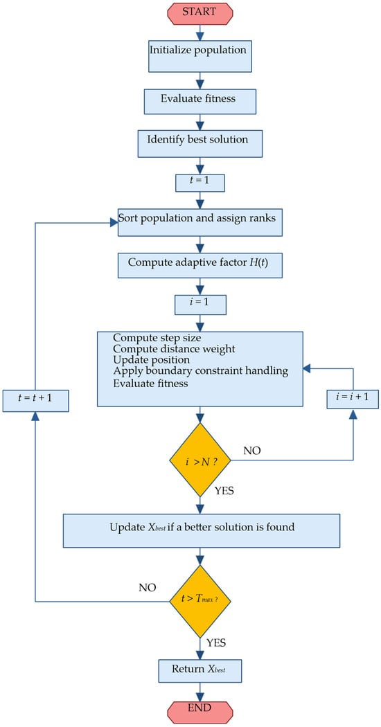
The logical flow of the proposed ICO algorithm is illustrated graphically in Figure 1. The algorithm begins with the random initialization of the cheetah population within the prescribed variable bounds, followed by fitness evaluation and identification of the current best solution. At each iteration, the population is sorted by fitness to enable rank-based step adaptation, and the adaptive parameter is computed to modulate the exploration-exploitation balance. For each individual cheetah, the position update incorporates leader-guided movement, distance-weighted interaction, and the rank-adapted step vector. Boundary constraints are enforced to maintain feasibility, and the population is re-evaluated to update the global best solution. This iterative process continues until the maximum number of iterations is reached, at which point the algorithm returns the optimal solution.
Figure 1.
Flowchart of the proposed Improved Cheetah Optimizer (ICO) algorithm.
The computational complexity of ICO is dominated by the fitness evaluations performed at each iteration. With a population size of and a maximum of iterations, the algorithm requires objective function evaluations. The additional operations associated with ranking, distance computation, and position updates contribute negligible overhead relative to the cost of evaluating the bi-level planning objective function, which requires solving the lower-level operational problem under wind uncertainty scenarios.
3.3. Integration of ICO with the Bi-Level Planning Framework
The ICO algorithm is employed to solve the upper-level planning problem defined in Section 2.2. Each cheetah in the population encodes a candidate planning solution comprising the installation buses and capacities of WBDG and BESS units. For each candidate solution, the following evaluation procedure is executed.
- First, the planning variables are decoded from the cheetah’s position vector. The discrete bus selection variables are rounded to the nearest integer and mapped to valid bus indices within the distribution network. The continuous capacity variables are directly interpreted as the installed capacities of WBDG and BESS units.
- Second, wind power uncertainty is characterized by using the Two-Point Estimation Method described in Section 2.7. For each WBDG unit, estimation points are generated according to Equations (20) and (21) based on the statistical moments of wind speed at the installation location. The available wind power for each estimation point is computed using the wind turbine power curve defined in Equation (25).
- Third, for each 2m-PEM estimation point, the lower-level operational optimization problem defined in Section 2.3, Section 2.4 and Section 2.5 is solved with the upper-level planning variables fixed. This involves determining the optimal BESS charging and discharging schedule over the 24 h horizon, satisfying the BESS constraints in Equations (12)–(16) and the network power flow constraints in Equations (17)–(19). Each scenario’s operating cost can be estimated at Equation (10).
- Fourth, the expected operational cost can be estimated using Equation (26), which is obtained based on the probability-weighted sum of scenario-wise operating cost estimates. The expected operating cost will then be combined with investment and maintenance cost components to compute the objective function of the upper-level planning as shown in Equation (1).
- Fifth, if there are any violations of the operational constraints in the lower-level analysis for a certain scenario, a large penalty is added to the objective function of the upper planning to avoid selecting an infeasible planning decision.
The ICO algorithm uses the search techniques as discussed in Section 3.2 to improve the quality of the population continuously until the termination condition is satisfied. In other words, when the ICO converges, the best solution produced by the ICO provides the optimal design decisions for the placement and sizing of WBDG and BESS units, which minimize the total cost and satisfy the operational feasibility constraint.
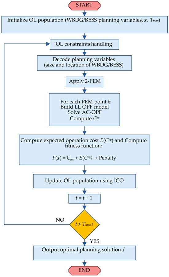
The whole procedure of implementing ICO along with the 2m-PEM is illustrated in Figure 2. As we can see in this figure, the first step of the integrated procedure involves initializing the ICO population. Next, the 2m-PEM creates several deterministic scenarios by perturbing the mean wind speed according to its distribution. Then, the operational schedule problems corresponding to the scenarios are solved to calculate their operating cost estimates. Afterward, the scenario-wise operating cost estimates are used to calculate the expected cost. With the expected operating cost, the upper-level objective function is calculated, and it will be assigned as the fitness of the corresponding cheetah. After that, the search processes in the ICO continue iteratively until they converge.
Figure 2.
Flowchart of the integrated ICO-2PEM bi-level solution algorithm for optimal WBDG and BESS planning under wind uncertainty.
4. Numerical Results and Discussion
The present section aims at conducting an elaborate mathematical analysis of the developed bi-level framework for the optimal allocation and capacity determination of WBDG and BESS under wind generation uncertainty. Wind generation uncertainty is modeled using the Two-Point Estimation Method (2m-PEM), as discussed in Section 2.7, whereas the solution to the upper-level planning problem is achieved using ICO, which is described in Section 3. For purposes of benchmarking, the efficiency of the ICO is evaluated against three established metaheuristic optimization techniques: Particle Swarm Optimization (PSO), Genetic Algorithm (GA), and traditional Cheetah Optimization Algorithm (CO). In terms of the goal of the optimization, the minimum cost function is minimized based on the total expected cost of operation over 24 h that incorporates the cost of energy purchased from the upstream grid and the financial equivalent of line losses in the distribution grid as given by Equation (10). The test study involves the use of the popular IEEE 33-bus radial distribution system, frequently used in distribution systems optimization literature. Implementation is carried out in the Matlab R2021b environment, with all three algorithms using identical parameters: population size is set at 30 agents, while the number of iterations is 100. To account for statistical significance in the presence of randomness involved in the working principles of metaheuristic algorithms, each technique is independently run 20 times.
4.1. Input Data and Uncertainty Representation
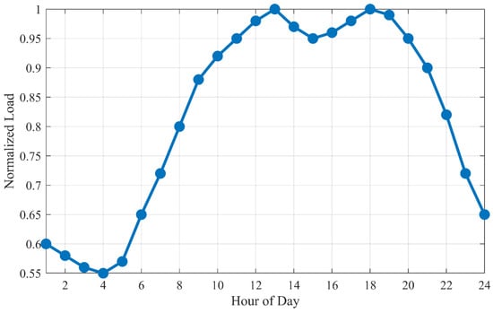
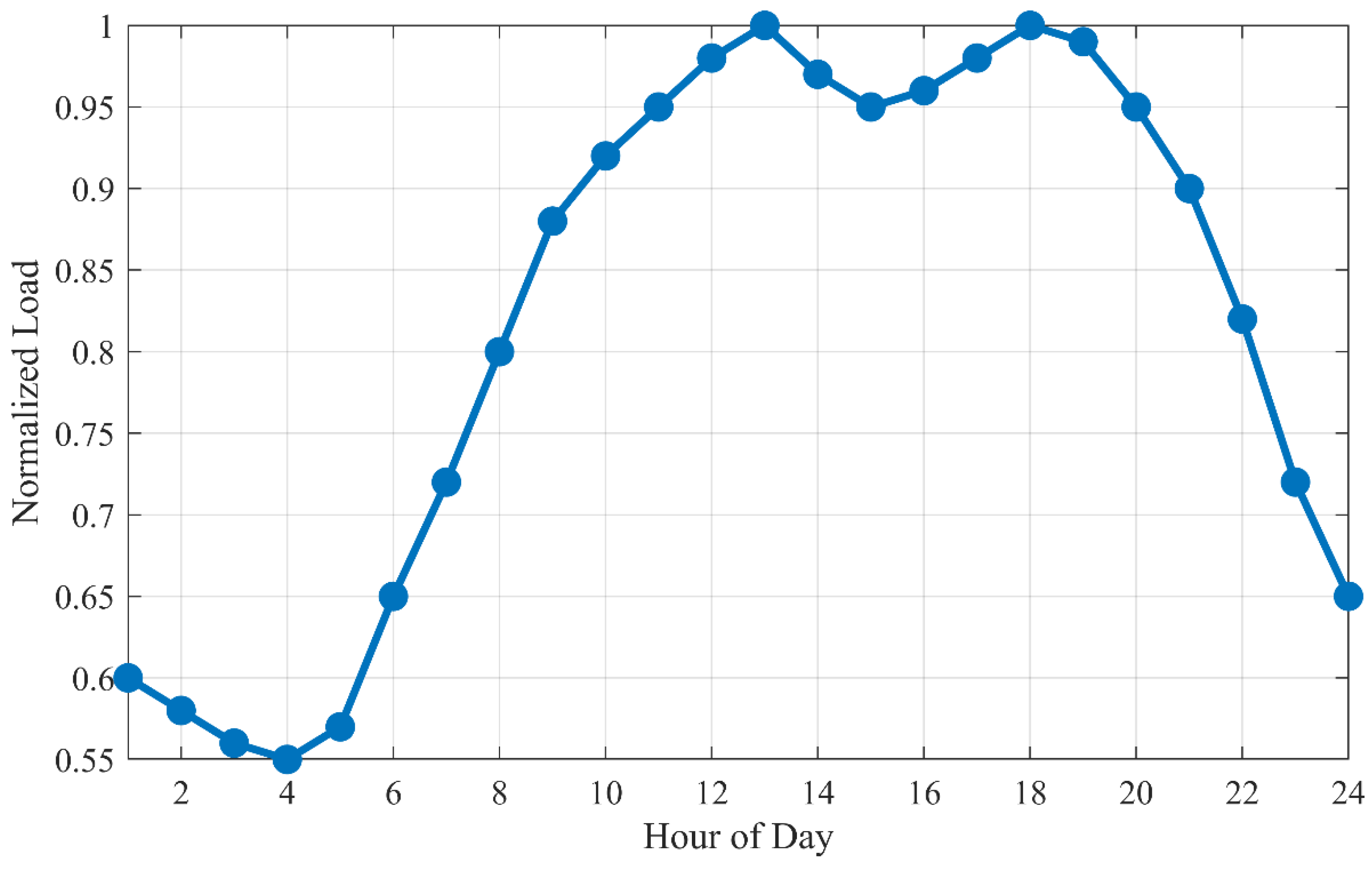
The time-dependent load curve adopted in our simulations is shown in Figure 3, where the normalized load variation in terms of hours per day is plotted. The chosen load curve reflects typical daily variations in loads that can be encountered in a distribution system, providing the basis for analyzing the operational performance throughout the scheduling horizon. The maximum power consumption is achieved during the evening, while the minimum is seen during the early mornings due to consumption patterns that are common for both residential and commercial sectors.
Figure 3.
Daily normalized load variation used in the simulation.
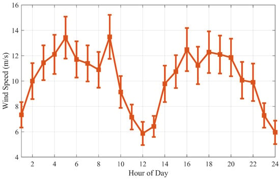
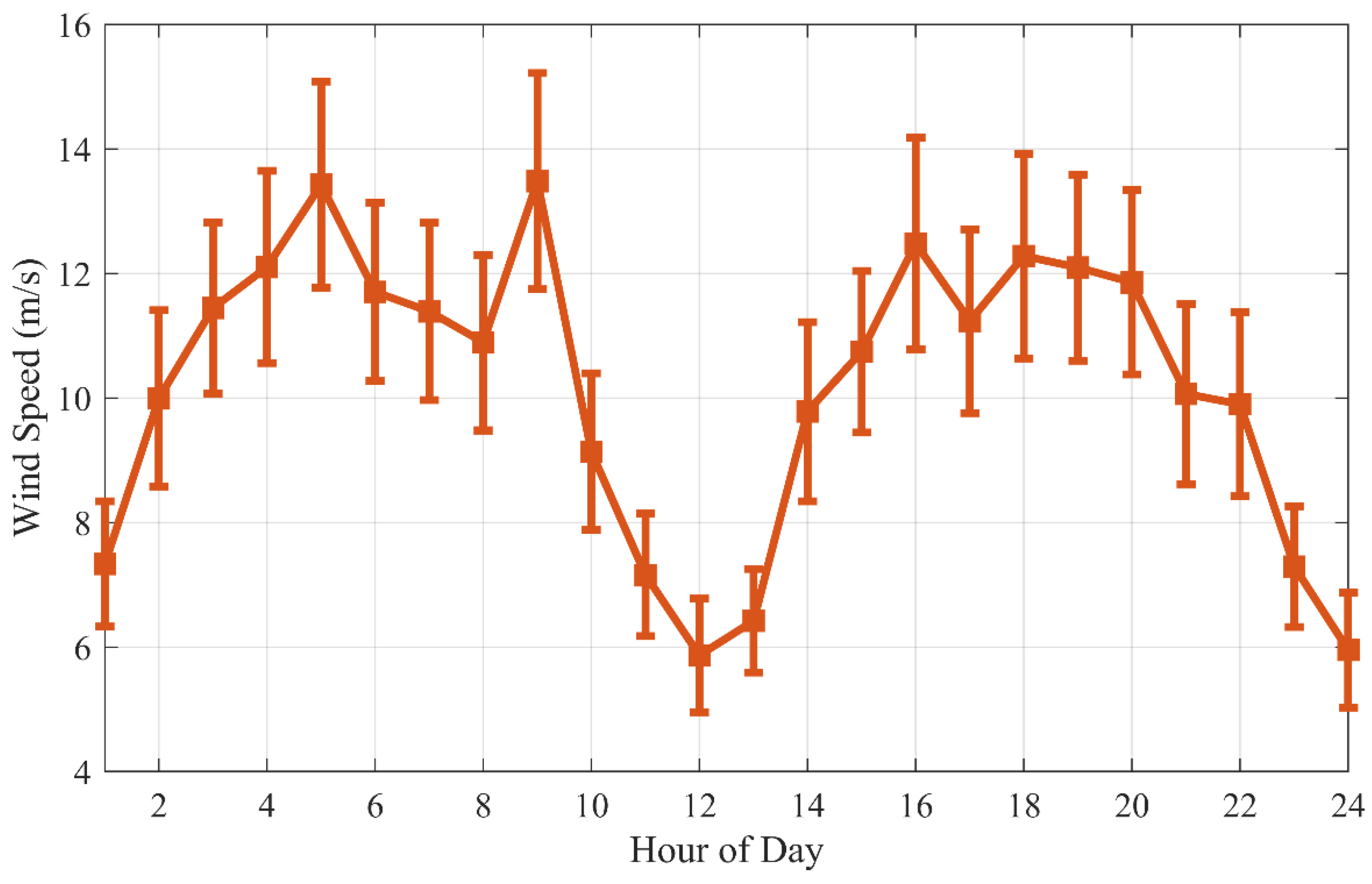
In order to represent the wind resource uncertainty, we use average values and standard deviations of hourly wind speeds as provided in Figure 4. These parameters are estimated based on historical data about wind speeds obtained in the region under consideration. The dataset used in this study consists of meteorological and environmental parameters obtained from a wind resource database in Riyadh for the period from 2013 to 2016 to represent realistic wind variability conditions. As follows from the figure, the average wind speed varies significantly depending on the hour of the day, being larger at daytime than at nighttime when less atmospheric mixing is expected. The average wind speed shows a significant diurnal variation, with the high values generally observed during the day, consistent with enhanced atmospheric mixing and heating effects.
Figure 4.
Hourly mean wind speed profile with corresponding standard deviation bands.
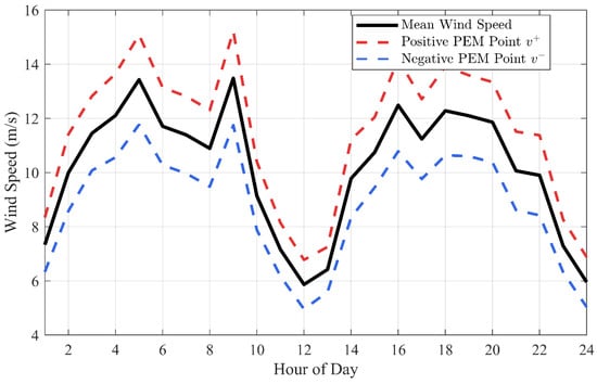
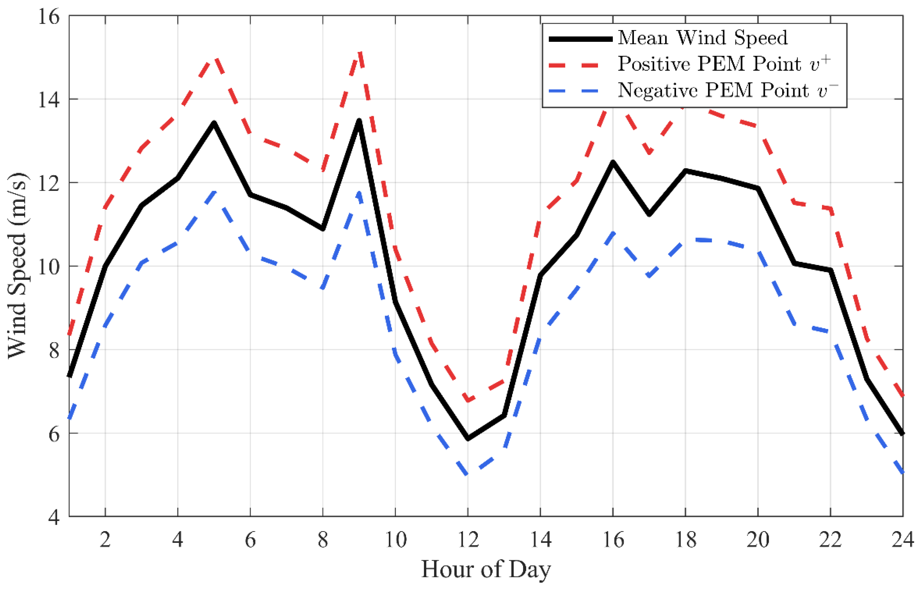
Instead of using Monte Carlo simulations that imply the generation of hundreds or even thousands of scenarios for each planning decision under consideration, we use the Two-Point Estimation Method outlined in Section 2.7 to approximate the stochastic behavior of wind speed. The above approach will lead to the creation of two deterministic wind cases labeled and , which are evenly spaced from the mean wind speed and reflect the probability distribution of the parameter as per Equations (20) and (21). The two cases are illustrated in Figure 5 and subsequently fed into the low-level operation planning optimization model to derive the expected results using the weighted sum formula of Equation (26).
Figure 5.
Wind speed scenarios generated using the Two-Point Estimation Method.
4.2. Statistical Performance of the Optimization Algorithms
The statistical outcomes after performing the algorithms independently twenty times have been summarized in Table 1 and Table 2. The best, average, standard deviation, and worst values for the expected cost of operations that can be obtained using PSO, GA, CO, and the proposed ICO algorithms are shown in Table 1. The expected operational cost is measured in United States dollars, which indicates the amount spent on the purchase of energy and loss compensation.
Table 1.
Statistical summary of expected operational cost obtained by different optimization algorithms over 20 independent runs.
Table 2.
Statistical summary of computational runtime obtained by different optimization algorithms over 20 independent runs.
From the examined approaches, the suggested ICO method yields the most advantageous optimization outcomes based on statistical measures. Namely, the optimal cost produced by ICO is equal to $5449.92, whereas its average cost is $5665.23. It is worth noting that the former metric is better than the results obtained with the help of other techniques by approximately 2.2%, whereas the latter measure surpasses those values by approximately 3.4%. In addition, the standard deviation value corresponding to the ICO algorithm is the lowest ($264.36).
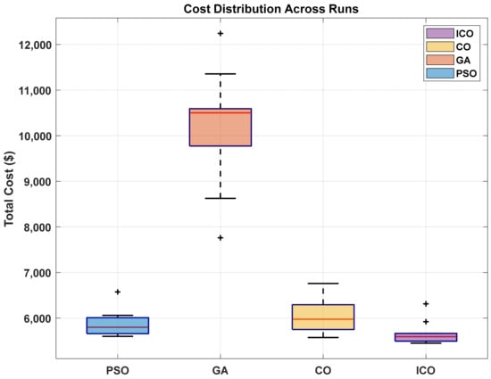
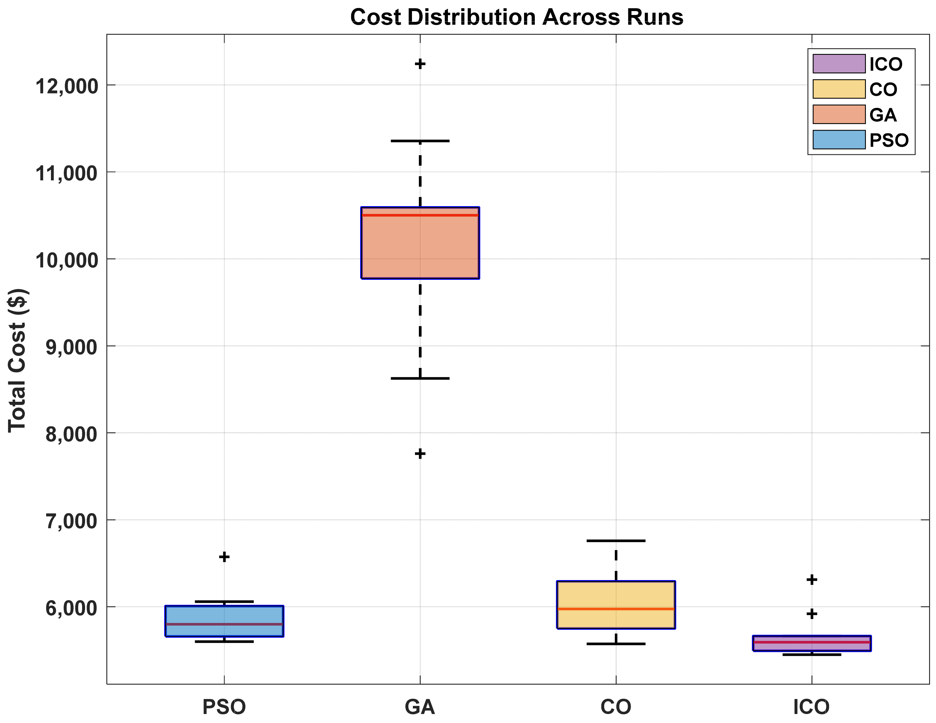
The following Figure 6 represents the box plot illustrating the distribution of the objective function values over the twenty independent runs performed by the four examined algorithms. The graph presents the median, interquartile range, and full range for the objective function costs achieved by each of the analyzed methods. The box plot analysis reveals multiple advantages of the suggested ICO approach in comparison with the examined alternative approaches. First, it can be noted that the median cost calculated for the proposed technique is inferior to those costs estimated for PSO, CO, and GA. The mean values of the objective functions evaluated for ICO were presented earlier in Table 1. Another advantage of the proposed algorithm lies in its robustness, which is reflected in the relatively narrow height of the box in comparison with that of the alternative approaches. In addition, the whiskers of the proposed algorithm are shorter than those of PSO and CO, which reflects the stability of the suggested technique under consideration. Conversely, the box plot corresponding to the GA algorithm is significantly elongated with extended whiskers, which indicates its substantial variability. It should be highlighted that the higher upper whiskers and outliers observed in PSO and CO box plots show that these algorithms tend to be trapped at some local optima from which they cannot move away. Thus, ICO is characterized by a decreased probability of being unable to find the solution in comparison with the competing techniques. This quality is critical to practical applications in power system planning due to the necessity to produce repeatable results. This phenomenon is explained by the use of advanced enhancements implemented in Section 3.2.
Figure 6.
Box plot comparison of expected operational cost distributions over 20 independent runs for PSO, GA, CO, and the proposed ICO algorithm.
The computational time performance statistics for all the considered algorithms are presented in Table 2, in seconds per run. According to Table 2, the mean runtime for PSO is about 26.52 s, while the mean runtime values for CO and ICO are around 24.03 s and 24.72 s, respectively. The slight increase in mean runtime for ICO compared to CO can be explained by extra computations associated with the enhancements discussed in Section 3.2, such as rank ordering, distance computation, and adaptation of parameters. Yet, the increase in computational time is absolutely justified in view of the high solution quality and robustness provided. At the same time, the GA demonstrates much greater computational performance issues, with the mean runtime reaching almost 979 s and the maximum runtime value exceeding 2125 s. It should be noted that the increased computational time performance of GA is determined by population handling procedures and a greater number of effective function evaluations necessary to reach convergence in the problem domain.
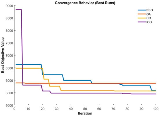
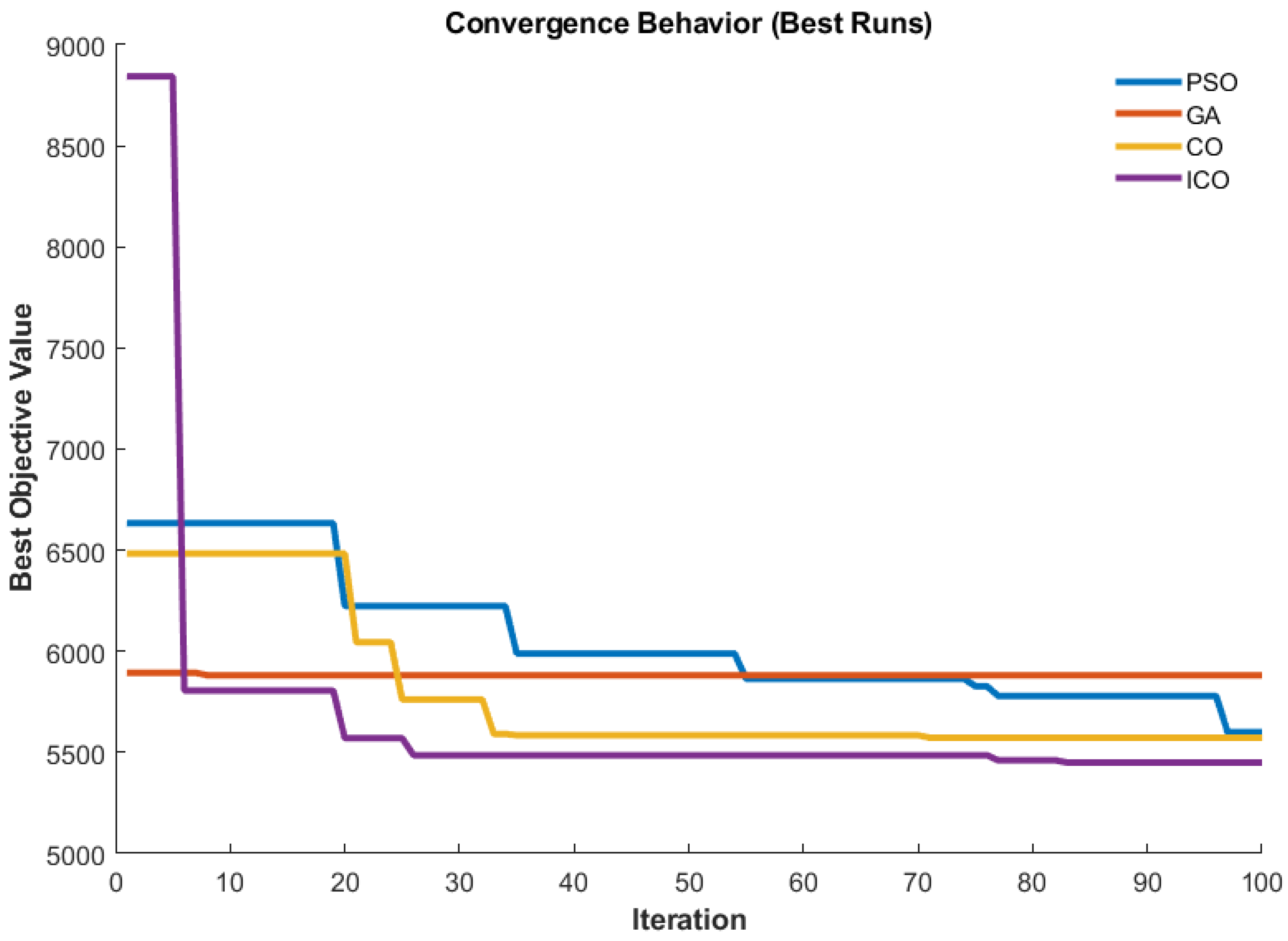
Additional insights into the convergence nature of the algorithms are offered by Figure 7, which provides a comparison between the changes in the best objective value achieved in relation to the iteration number for one exemplary run of each algorithm. It is evident that ICO shows much faster convergence during the first stages and achieves a final solution that is characterized by a better cost value than those provided by the competitors. The improved convergence rate is due to the introduction of the leader-guided search procedure, as formulated in Equation (34) and the step update rule presented in Equation (35). Both strategies enable the swarm to approach promising areas in the search space in an efficient manner. In turn, PSO and CO also show appropriate convergence properties but are finally trapped in local optima of the problem, which leads to obtaining worse solutions. Moreover, GA is characterized by substantially slower convergence and higher oscillations within the optimization process.
Figure 7.
Convergence curves of PSO, GA, CO, and ICO for the bi-level planning optimization problem.
Ablation Study: Contribution of Each ICO Enhancement
To quantify the contribution of each modification in the proposed ICO, an ablation study was performed. Four variant algorithms were created by removing one enhancement at a time: ICO-noLGS (without leader-guided search), ICO-noRSA (without rank-based step adaptation), ICO-noDWI (without distance-weighted interaction), and ICO-noAB (without adaptive exploration-exploitation balance). Each variant, together with standard CO and full ICO, was executed in 20 independent runs on the same bi-level planning problem (IEEE 33-bus system with wind uncertainty). Table 3 summarizes the results.
Table 3.
Ablation study results (best cost, mean cost, standard deviation, and improvement over CO).
All ablation variants outperform standard CO, confirming that each enhancement provides a positive effect. Distance-weighted interaction (DWI) contributes the most; removing it (ICO-noDWI) raises the best cost to $5518.33, losing about 55% of the total improvement achieved by ICO over CO. Adaptive balance (AB) and rank-based step adaptation (RSA) also contribute significantly, with best costs of $5530.62 and $5535.48, respectively. Leader-guided search (LGS) contributes the least but still improves upon CO (best cost $5560.15). The four enhancements work synergistically, as removing any single one reduces performance, and the full ICO achieves the best solution quality and robustness.
4.3. Optimal Planning Results
Table 4 highlights the optimal allocation and sizing of the WBDG units and BESS determined using the competing algorithms. These findings show that there are significant disparities between the optimal planning techniques generated by the algorithms due to their differing abilities to examine the problem space and determine optimal solutions.
Table 4.
Optimal placement and sizing of WBDG and BESS units obtained by different optimization algorithms.
The PSO algorithm locates the wind turbines on buses 22, 17, and 9, with their capacities being 1.13 MW, 1.25 MW, and 1.40 MW, respectively, and the placement of BESS units is established at buses 16 and 19, with capacities of 0.59 MW and 0.65 MW, respectively. This indicates that there is an acceptable spatial deployment of the energy sources along the distribution feeder. The CO algorithm locates the wind generators on buses 26, 2, and 3, and places the three BESS units at buses 29, 23, and 13. While this solution achieves a lower cost than PSO, the placement of multiple BESS units with relatively small energy capacities may limit the operational flexibility provided by storage. In the case of the GA, however, only wind generation facilities are employed without any BESS allocation, which suggests that the proposed algorithm failed to capitalize on the inherent advantages that can be gained from energy storage in terms of flexibility and economics. The absence of BESS facilities results in a significantly higher operational cost and increased variability of the GA solution, as shown in Table 1 and Figure 6.
On the other hand, the ICO algorithm yields a more balanced and economical solution. The optimal combination for the ICO algorithm consists of three wind generation facilities, which have been allocated at buses 4, 2, and 18, with rated powers of 1.34 MW, 1.50 MW, and 1.50 MW, respectively. Two BESS facilities have been assigned to buses 10 and 33, with power capacities of 0.37 MW and 0.98 MW, and energy capacities of 1.50 MWh and 3.15 MWh, respectively. The proposed combination has some advantages. For example, wind generation facilities have been dispersed among various parts of the distribution line, which means that power generation will not be concentrated at one point, thus mitigating any possible problems related to voltage increase. Furthermore, BESS facilities have been allocated in key positions. Specifically, the facility with higher power has been placed on the distant bus 33, which provides adequate voltage support. Finally, the energy-to-power ratio of each BESS facility is approximately 4.05 h and 3.21 h, respectively, allowing enough time for wind energy production to shift its schedule from low-demand to high-demand times.
4.4. Base Case and Optimized Network Comparison
A comparative study of the base network performance in the absence of renewable resources and storage, as well as the optimized system performances resulting from each of the algorithms, is shown in Table 5. In the base scenario, the network suffers energy losses of 2.2577 MWh/day, and the lowest bus voltage magnitude becomes equal to 0.9440 p.u., almost reaching the lower limit of operation, usually imposed in distribution networks, which equals 0.95 p.u. The incorporation of optimized renewable resources results in substantial technical improvement.
Table 5.
Comparative analysis of base case and optimized solutions for different algorithms.
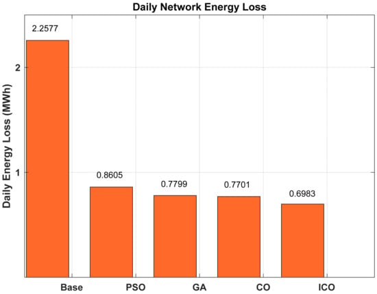
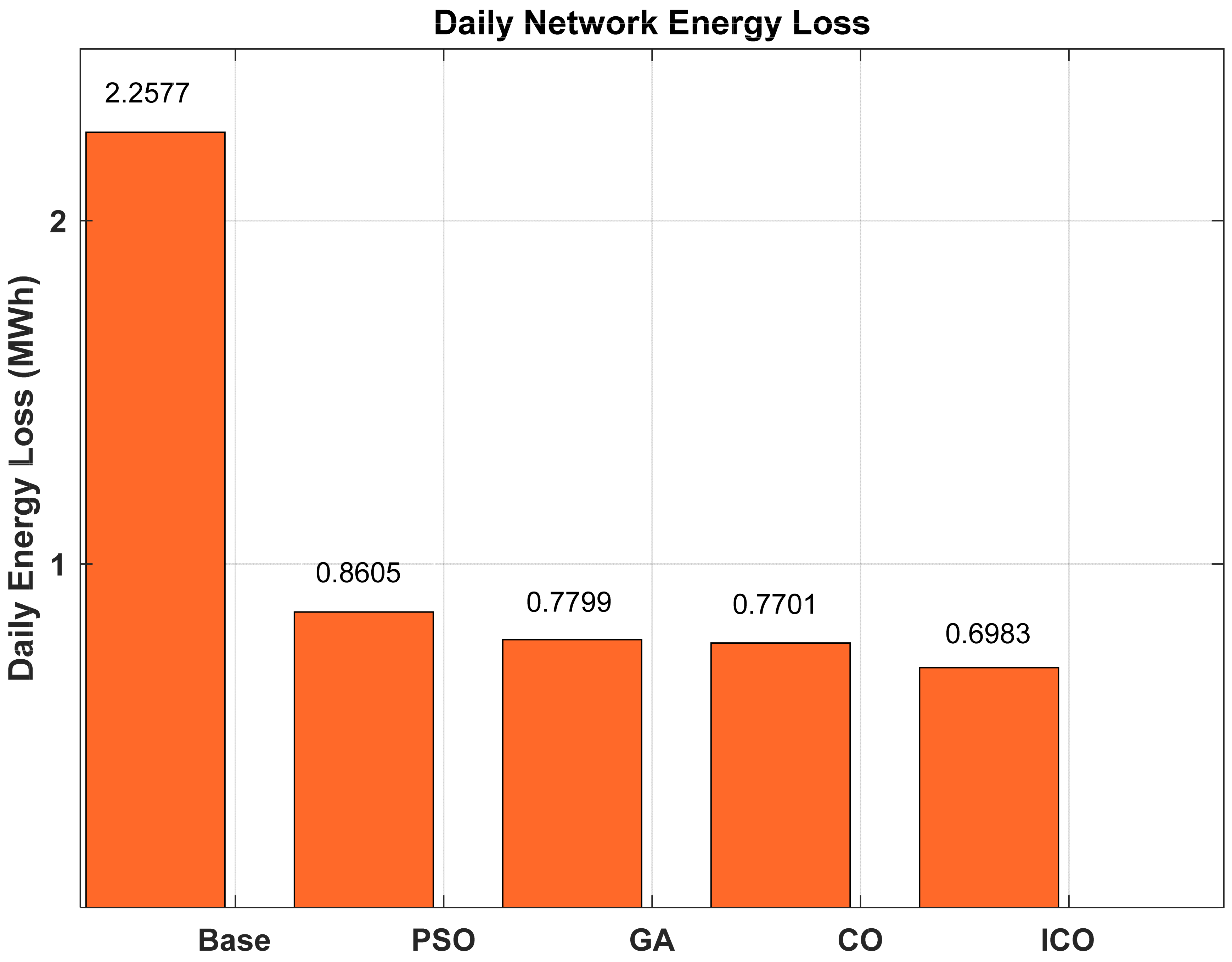
Comparatively, ICO attains the greatest loss reduction among all of the evaluated algorithms. As such, the energy loss per day is reduced to 0.6983 MWh, representing a loss reduction of 69.07% against the baseline loss. The next best algorithm after ICO in terms of energy losses is CO, which reduces losses by 65.89%. Following this, PSO achieves energy losses of about 61.89%, followed by GA, which cuts losses by 65.46%. Notably, the GA loss reduction is done at a considerably higher operational cost compared to other algorithms because of the suboptimal resource allocation scheme used in the GA solution and the exclusion of BESS from the optimal solution. As mentioned above, the GA allocation scheme requires additional grid imports for load demand satisfaction during low wind availability.
Another notable benefit of integrating WBDG and BESS units into the network is the improvements realized in terms of voltage performance. Specifically, voltage magnitudes are improved such that their lowest value exceeds 0.957 per unit, showing an average improvement of more than 1.30%. In this regard, the ICO solution attains the greatest minimum voltage magnitude, at 0.9610, representing an improvement of about 1.80%. This is impressive considering the constraint conditions on voltage magnitudes in a distribution system. Voltage magnitudes cannot exceed the upper limit nor be less than the minimum allowable voltage magnitudes to guarantee stable power flow without violating voltage boundaries during contingencies.
From an economic point of view, the best algorithm for planning purposes is ICO because of the relatively lower operational cost it offers. The total operational cost attained via the use of ICO is $5449.92, representing an annual cost lower than the cost obtained using CO ($5572.79), PSO ($5600.15), and GA ($7761.25). The difference in cost between the best performer, ICO, and the second-best performer, CO, stands at about $122.87 per day, equivalent to $44,850 annually.
4.5. Voltage and Loss Profile Analysis
To illustrate the advantages associated with the optimized planning model, Figure 8 shows the results comparing the daily energy losses between the base case scenario and the optimized scenarios derived through each of the four algorithms. It is evident from Figure 8 that all of the optimization models show a marked improvement in energy losses compared with the base scenario, where ICO achieves the greatest reduction in both numerical and percentage terms. This loss reduction is a result of two factors working in tandem: the local injection of power by WBDG systems decreases the amount of power transmission from the substation, and energy shifting by BESSs optimizes energy generation locally with respect to demand.
Figure 8.
Comparison of daily network energy losses for Base, PSO, GA, CO, and ICO solutions.
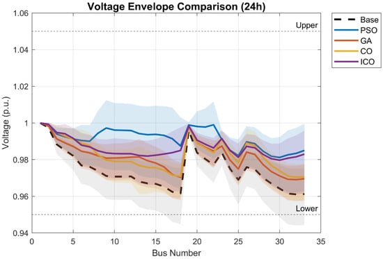
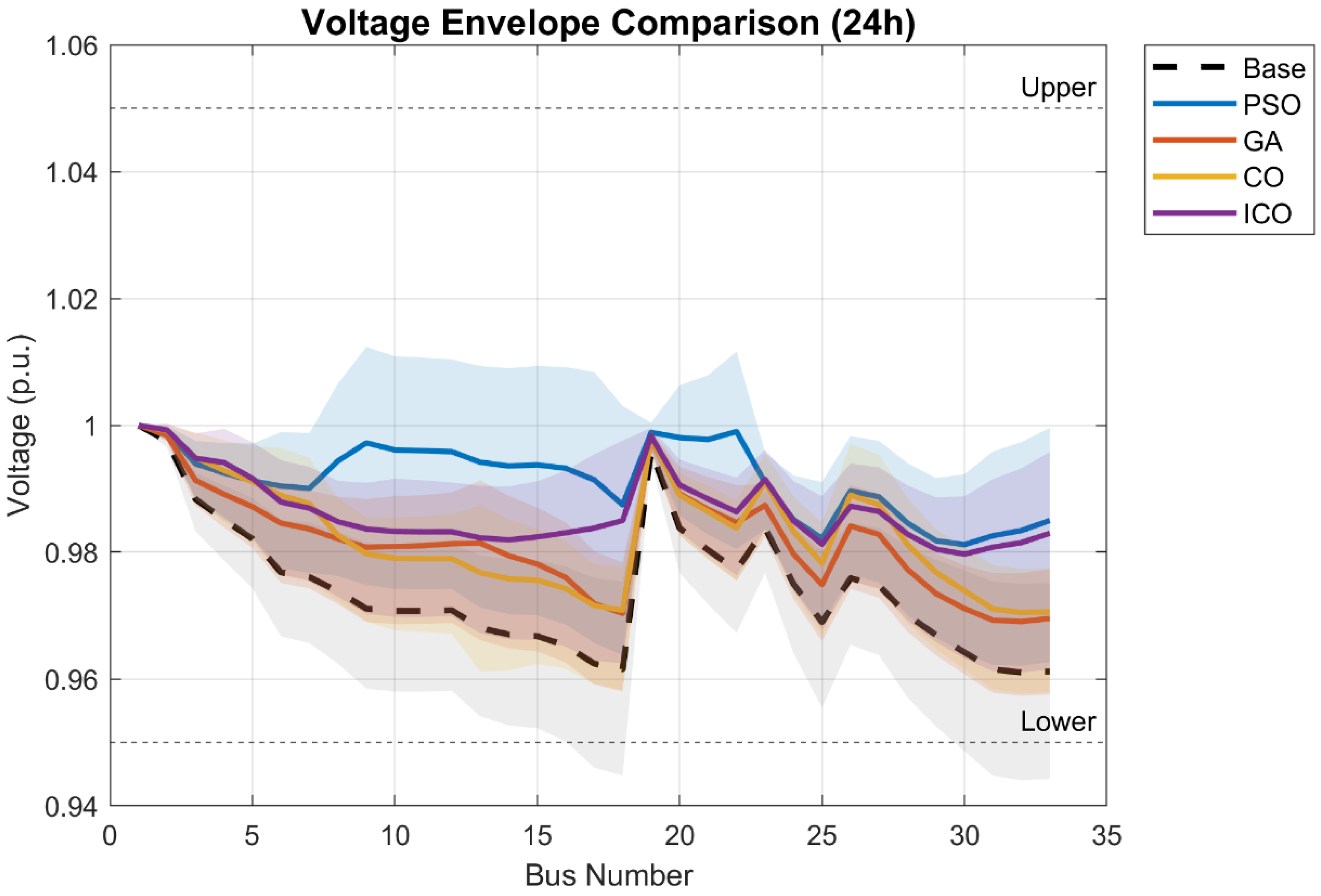
Figure 9 shows the magnitude of the voltages on all the buses under peak conditions. The base case shows a decreasing trend in the voltage magnitudes throughout the feeder due to the cumulative effect of line impedances and the current load. The voltage levels reach their lowest levels at the buses furthest away from the substation, close to their operating limits. However, after installing the optimized WBDG and BESS placements, the voltage profiles are much flatter, staying within their permissible ranges of operation. The impact is especially noticeable in the buses at the extreme ends of the feeder network since their voltage levels benefit from the presence of local sources of energy and energy storage systems. The ICO approach results in a constant voltage profile, implying the optimal placement of power generators and energy storage facilities.
Figure 9.
Voltage magnitude profile of the IEEE 33-bus system for base and optimized cases under peak load conditions.
4.6. Discussion
The numerical results presented below clearly confirm the viability of the proposed ICO-based planning framework in the context of wind-powered distribution networks. Indeed, the increased optimization capabilities of ICO, stemming from the four improvements discussed in Section 3.2, allow detecting configurations with lower expected operational cost and power losses in comparison with PSO, GA, and classical CO. The ability to combine wind generation and BESS enables adjusting to possible variations in wind generation while keeping voltage within the required range and improving overall power quality. Optimal allocation of generation and energy storage devices allows leveraging the synergy provided by those two components by installing wind generators at renewable-rich locations and locating BESS at places where they will provide the greatest impact on voltage and power losses minimization.
There are several important findings made during the comparison of approaches. First, it should be noted that energy storage units play a crucial part not only in terms of minimizing power losses but also in reducing operational costs. As can be seen from Table 1 and Figure 6, the solution generated by the GA did not take into account the presence of BESS; consequently, even though it was comparable in terms of loss minimization, the GA solution led to greater average operational costs. Second, it is evident that proposed enhancements have improved ICO, as it performed better than the basic version of CO. Third, the application of box plot diagrams in the comparative analysis reveals the advantages of using ICO, as the interquartile range for this algorithm is smaller than for other approaches, and whiskers are shorter, which indicates less variability and more robust results obtained independently of stochastic factors affecting initialization and search process.
Another finding is the applicability of the 2m-PEM approach in addressing uncertainty related to the stochastic nature of wind power. The introduction of just 2m deterministic scenarios when solving this problem allows obtaining an approximate estimation of the true probabilistic distribution, which is a reasonable trade-off considering that the computational complexity associated with this approach remains acceptable.
The obtained results in terms of the achieved savings—about a 69% reduction in energy losses per day together with the lowest average operational cost among all used methods and higher statistical robustness—show promising perspectives of employing the proposed framework for planning the future distribution systems with renewables. The methodology developed in this paper provides a useful tool for selecting the most optimal locations of wind generators and energy storage devices based on realistic scenarios and taking into consideration both economic aspects and technical limitations.
4.7. Summary of Key Findings
The main results of the numerical case study are presented below. In comparison with PSO, GA, and classical CO, the proposed ICO algorithm shows the best performance in all aspects considered. This allows finding a solution that minimizes the expected value of daily operating cost at the level of $5449.92, with the standard deviation being equal to $264.36 within 20 independent executions. Analysis of the box plot also demonstrates the increased robustness of ICO due to its smaller interquartile range and variance in comparison with other algorithms. Using ICO leads to obtaining a planning strategy that provides a decrease in daily energy loss of 69.07% along with a higher minimum voltage on buses, increasing it from 0.9440 to 0.9610 p.u. Computational efficiency of the method considered remains comparable with PSO and CO at the level of 24.72 s. Thus, ICO works 40 times faster than GA. Using the 2m-PEM allows accounting for the effect of uncertainty associated with renewable generation on the basis of wind resources in the bi-level problem. It should be noted that the combined application of WBDG and BESS is important for reaching an optimal solution in the studied case due to its high expected cost.
4.8. Sensitivity Analysis of BESS Degradation
In the main study, BESS degradation (capacity fade over time) was not modeled. To assess the potential impact of this omission, we perform a post-optimization sensitivity analysis. A typical lithium-ion battery experiences approximately 5% annual capacity fade under standard cycling conditions. Over a 10-year planning horizon, this reduces the effective energy capacity to about 60% of its rated value. To capture this effect, we re-evaluate the optimal BESS capacity obtained by ICO (3.15 MWh at bus 33, 1.50 MWh at bus 10) under a simplified degradation model: the effective available energy is reduced by 5% per year, and the annualized investment cost is increased by a degradation factor (5% annual capacity loss translated into a 2.5% increase in equivalent annual cost). The results are summarized in Table 6.
Table 6.
Impact of BESS degradation on optimal planning outcomes.
Including degradation leads to larger BESS capacities (approximately 12% increase) to compensate for capacity fade and a modest increase in operational cost (8%). The minimum voltage and loss reduction remain close to the non-degradation case, and the relative performance of ICO compared to other algorithms remains unchanged. Thus, while degradation is an important practical consideration, its omission does not invalidate the main conclusions of this study. A full degradation-aware optimization is left for future work.
5. Conclusions
This study introduced a bi-level optimization framework for the coordinated planning of wind-based distributed generation (WBDG) and battery energy storage systems (BESS) in radial distribution networks under wind power uncertainty. Wind variability was modeled using the Weibull distribution and the Two-Point Estimation Method (2m-PEM), while an Improved Cheetah Optimizer (ICO) was developed to efficiently solve the resulting mixed-integer, nonlinear bi-level problem. The ICO incorporates leader-guided search, rank-based step adaptation, distance-weighted interaction, and an adaptive exploration-exploitation balance to enhance convergence and robustness. The proposed framework was evaluated on the IEEE 33-bus system through 20 independent runs, with performance benchmarked against PSO, GA, and conventional CO. ICO generated the optimal results, having produced the lowest expected cost of operation at $5449.92 and mean cost at $5665.23 with a standard deviation of $264.36. Box plot analysis confirmed the reduced variability of ICO compared to competing algorithms. Daily energy losses were reduced by 69.07%, from 2.2577 MWh to 0.6983 MWh, and the minimum bus voltage improved from 0.9440 p.u. to 0.9610 p.u. The optimal configuration placed WBDG units at buses 4, 2, and 18 and BESS units at buses 10 and 33. In the case of the GA approach, where the BESS was not used, the expected cost of operation was relatively high. This shows the importance of storage when aiming to have an economical and efficient operation. It is confirmed that using the combination of probabilistic modeling of wind, bi-level decision making and advanced metaheuristic generates the optimal solution. Furthermore, a sensitivity analysis on BESS degradation (5% annual capacity fade) showed that optimal capacities increase by approximately 12% and operational cost by 8%, but the relative performance of ICO remains unchanged. Future work may further extend the proposed framework by simultaneously considering wind and load demand uncertainties, in addition to incorporating photovoltaic generation, reactive power support, unbalanced network conditions, and degradation-aware BESS modeling for multi-year planning horizons.
Author Contributions
Conceptualization, S.A. and A.S.A.; methodology, S.A. and A.S.A.; software, S.A.; validation, S.A. and A.S.A.; formal analysis, S.A.; investigation, S.A.; resources, S.A. and A.S.A.; data curation, S.A.; writing—original draft preparation, S.A. and A.S.A.; writing—review and editing, A.S.A.; visualization, A.S.A.; supervision, A.S.A.; project administration, A.S.A.; funding acquisition, A.S.A. All authors have read and agreed to the published version of the manuscript.
Funding
The author extends their appreciation to the deputyship for Research & Innovation, Ministry of Education in Saudi Arabia for funding this research work through the project number (IFP-2022-2026-275).
Data Availability Statement
The original contributions presented in this study are included in the article.
Acknowledgments
The author extends their appreciation to the deputyship for Research & Innovation, Ministry of Education in Saudi Arabia for funding this research work through the project number (IFP-2022-2026-275).
Conflicts of Interest
The authors declare no conflicts of interest.
References
- Balogh, J.M.; Mizik, T. Global Impacts of Climate Policy and Trade Agreements on Greenhouse Gas Emissions. Agriculture 2023, 13, 424. [Google Scholar] [CrossRef] [Scilit]
- Wang, Y.; Liu, Y.; Gu, B. COP26: Progress, Challenges, and Outlook. Adv. Atmos. Sci. 2022, 39, 1209–1216. [Google Scholar] [CrossRef] [Scilit] [PubMed]
- Zou, X. India’s Climate Path: Balancing Development Rights with Environmental Accountability BT. In Thirty Years of Global Climate Governance: From Rio to Glasgow; Zou, X., Ed.; Springer Nature: Singapore, 2026; pp. 83–98. ISBN 978-981-95-8457-4. [Google Scholar]
- Mehigan, L.; Deane, J.P.; Gallachoir, B.Ó.; Bertsch, V. A review of the role of distributed generation (DG) in future electricity systems. Energy 2018, 163, 822–836. [Google Scholar] [CrossRef] [Scilit]
- Hung, D.Q.; Mithulananthan, N.; Bansal, R.C. Integration of PV and BES units in commercial distribution systems considering energy loss and voltage stability. Appl. Energy 2014, 113, 1162–1170. [Google Scholar] [CrossRef] [Scilit]
- Medina, A.C.R.; Franco, J.F.; Rider, M.J.; Feltrin, A.P.; Romero, R. A mixed-integer linear programming approach for optimal type, size and allocation of distributed generation in radial distribution systems. Electr. Power Syst. Res. 2013, 97, 133–143. [Google Scholar] [CrossRef] [Scilit]
- Singh, B.; Sharma, J. A review on distributed generation planning. Renew. Sustain. Energy Rev. 2017, 76, 529–544. [Google Scholar] [CrossRef] [Scilit]
- Kwangkaew, A.; Javaid, S.; Charoenlarpnopparut, C.; Kaneko, M. Optimal location and sizing of renewable distributed generators for voltage stability and security. Energies 2022, 15, 2126. [Google Scholar] [CrossRef] [Scilit]
- Das, S.K.; Sarkar, S.; Bhattacharya, A. Optimal allocation of PV-based DG and scheduling of BESS in a grid-connected microgrid using bi-level optimisation. SN Comput. Sci. 2023, 4, 588. [Google Scholar] [CrossRef] [Scilit]
- Bawazir, R.O.; Cetin, N.S. Comprehensive overview of optimizing PV-DG allocation in power system and solar energy resource potential assessments. Energy Rep. 2020, 6, 173–208. [Google Scholar] [CrossRef] [Scilit]
- Samala, R.K.; Kotapuri, M.R. Optimal allocation of distributed generations using hybrid technique with fuzzy logic controller radial distribution system. SN Appl. Sci. 2020, 2, 191. [Google Scholar] [CrossRef] [Scilit]
- El-Ela, A.A.A.; Allam, S.M.; Shaheen, A.M.; Nagem, N.A. Optimal allocation of biomass DG in distribution systems using equilibrium algorithm. Int. Trans. Electr. Energy Syst. 2021, 31, e12727. [Google Scholar]
- Pereira, L.D.L.; Yahyaoui, I.; Fiorotti, R.; Menezes, L.S.D.; Fardin, J.F.; Rocha, H.R.O.; Tadeo, F. Optimal allocation of DG and capacitor banks using probabilistic models with correlations. Appl. Energy 2022, 307, 118097. [Google Scholar]
- Khasanov, M.; Kamel, S.; Houssein, E.H.; Rahmann, C.; Hashim, F.A. Optimal allocation strategy of PV and wind-based DG considering uncertainty. Neural Comput. Appl. 2023, 35, 2883–2908. [Google Scholar]
- Akbari, M.A.; Zare, M.; Azizipanah-Abarghooee, R.; Mirjalili, S.; Deriche, M. The Cheetah Optimizer: A nature-inspired metaheuristic algorithm for large-scale optimization problems. Sci. Rep. 2022, 12, 10953. [Google Scholar] [PubMed]
- Tye, M.R.; Stephenson, D.B.; Holland, G.J.; Katz, R.W. A Weibull approach for improving climate model projections of tropical cyclone wind-speed distributions. J. Clim. 2014, 27, 6119–6133. [Google Scholar] [CrossRef] [Scilit]
- Serban, A.; Paraschiv, L.S.; Paraschiv, S. Assessment of wind energy potential based on Weibull and Rayleigh distribution models. Energy Rep. 2020, 6, 250–267. [Google Scholar] [CrossRef] [Scilit]
- Aslam, M. Testing average wind speed using sampling plan for Weibull distribution under indeterminacy. Sci. Rep. 2021, 11, 7532. [Google Scholar] [CrossRef] [Scilit] [PubMed]
- Alizadeh, M.J.; Kavianpour, M.R.; Kamranzad, B.; Etemad-Shahidi, A. A Weibull distribution–based technique for downscaling of climatic wind fields. Asia-Pac. J. Atmos. Sci. 2019, 55, 685–700. [Google Scholar]
- Teimourian, H.; Abubakar, M.; Yildiz, M.; Teimourian, A. A comparative study on wind energy distribution models: A case study on Weibull distribution. Energies 2022, 15, 5684. [Google Scholar] [CrossRef] [Scilit]
- Hong, H.P. An efficient point estimate method for probabilistic analysis. Reliab. Eng. Syst. Saf. 1998, 59, 261–267. [Google Scholar] [CrossRef] [Scilit]
- Roy Ghatak, S.; Sannigrahi, S.; Acharjee, P. Optimised planning of distribution network with photovoltaic system, battery storage, and DSTATCOM. IET Renew. Power Gener. 2018, 12, 1823–1832. [Google Scholar] [CrossRef] [Scilit]

Disclaimer/Publisher’s Note: The statements, opinions and data contained in all publications are solely those of the individual author(s) and contributor(s) and not of MDPI and/or the editor(s). MDPI and/or the editor(s) disclaim responsibility for any injury to people or property resulting from any ideas, methods, instructions or products referred to in the content. |
© 2026 by the authors. Licensee MDPI, Basel, Switzerland. This article is an open access article distributed under the terms and conditions of the Creative Commons Attribution (CC BY) license.