


Abstract
This study addresses the multi-objective optimization of characterizing a flat glass processing plant. To assess the operational conditions required for a flat glass processing small and medium-sized enterprise (SME) to become a prosumer compatible with renewable energy community (REC) participation. This work is motivated by the presence of more than 300 SMEs in Italy, like this, where RECs represent one of the few viable strategies for achieving the European Union’s 2050 decarbonization targets. The research is carried out in two scenarios; Scenario-I includes Stage-i and Stage-ii with the mutual goal of forecasting and optimizing. Forecasting is used in Stage-i to optimize the factory load, and in Stage-ii to shift and curtail energy loads based on the forecast, considering the Italian national energy price and the regional price bands (“fasce orarie”) F1, F2, and F3. Forecasting and the indicators of environmental and social performance are the means to ensure the best energy utilization and management, as they prove that the reduction in CO2 emissions and benefits on the community level can be both obtainable. Subsequently, the techno-economic analysis and evaluation of prosumer-readiness conditions are carried out through the optimization of industrial energy demand: three optimization objectives are assessed in this study (i) energy cost, (ii) carbon emission, and (iii) load curtailment. Four algorithms are put into effect to solve the tri-objective optimization: multi-objective particle swarm optimization (MOPSO), multi-objective ant nesting algorithm (MOANA), non-dominated sorting genetic algorithm (NSGA-II), and multi-objective grey wolf optimization (MOGWO). The algorithms are validated in Stage-ii to find the desired optimum in the cost of energy, reduce peak formation, and carbon emissions. To achieve this goal, a stochastic approach based on Monte Carlo simulations and VIKOR is used to optimally select the results. The findings show that the NSGA-II, MOPSO, and MOANA are more effective in solving the problem, while the MOGWO algorithm more quickly finds the optimal solution. Based on the defined objectives, a new configuration for the energy community is introduced, together with a community well-being index and an evaluation of the resulting benefits for the factory. In Scenario-II, the PV plants’ installation on the factory is sized, and the excess energy shared with the grid is evaluated. The Scenario-II results show that 497.184 MWh (33.9%) of energy is shared with the grid. Both results suggest how optimized industrial demand profiles improve SME participation in future RECs.
1. Introduction
The ambitious target of the European Union to achieve climate neutrality by 2050, stated in the context of the European Green Deal [1], creates enormous challenges to energy-consuming industries. Specifically, the glass industry is cited as a hard-to-abate energy consumer due to its massive thermal power requirements, continuous production processes, and because it relies on fossil fuels in operating its furnaces [2]. The input of small and medium-sized enterprises (SMEs) involved in flat glass processing (cutting, tempering, laminating, and insulating) is often not considered in the studies of industrial decarbonization. These organizations are key players in the downstream value chain of the glass industry, particularly in the building and automotive industries. However, SMEs tend to have poor access to the technologies and the policy incentives needed for decarbonization due to having limited technical and financial resources [3].
Current studies are mainly focused on furnace-level energy accounting and carbon footprint reduction; Atzori et al. [4,5] analyzed the effect of CO2 reducing technologies in the hollow glass industry. Atzori et al. [6,7] have also more recently reviewed a national-scale roadmap to the decarbonization of the Italian glass industry and melting furnaces, highlighting the importance of integration of hydrogen use and electrification in the production process. Nevertheless, the decarbonization pathway specific to glass SMEs is still underdeveloped, as reported by Papadogeorgos and Schure [8]. Despite numerous studies dealing with energy optimization, electrification, and the fuel-switching strategy in large-scale glass production, significant knowledge gap areas are still present in smaller companies of the glass production industry [4,5,6,7]. Bracale et al. [9], developing linear regression models calibrated on a manufacturing plant in Italy, revealed that an accurate forecast of industrial load can be obtained through the introduction of work time shifts and production schedules. Zhu et al. [10] suggested a hybrid firefly algorithm-based forecasting model to optimize the extreme machine learning and adaptive boosting algorithm (LCR-AdaBoost-FA-ELM). It produced significant decreases in mean absolute percentage error in furniture manufacturing prediction. A modular artificial neural network (ANN)-based forecasting framework in smart grids (SGs) was proposed by Ahmad et al. [11], and an improved, high-precision, fast-convergent forecasting model was proposed by Ahmad et al. [12]. Similarly, Rehman et al. [13] and Corasaniti et al. [14] emphasized the connection between the integration of renewable energy sources, renewable energy communities (RECs), SGs, and modern energy systems in order to strengthen their socio-economic applicability and sustainability. The central role in industrial energy management is carried out through wholesale electricity pricing mechanisms, such as the Italian single national price “prezzo unico nazionale (PUN)” [15]. Moreover, Zapata [16] provides a panel-based analysis for renewable energy in remote indigenous communities and provides a well-being index in Canada to show the importance of renewable energy sources integration. Multi-objective optimization (MOO) of SGs integrating renewable sources is becoming the preferred approach to modern energy use. Ullah et al. [17] developed a tri-objective optimization model incorporating hybrid demand response and renewable energy source inclusion. This model involves the multi-objective particle swarm optimization (MOPSO) and a non-dominated sorting genetic algorithm II (NSGA-II), together with multi-objective wind-driven optimization (MOWDO) algorithms. Rashed et al. [18] presented the multi-objective ant nesting algorithm (MOANA) with adaptive exploration-exploitation strategies. Mengelkamp et al. [19] investigated blockchain-enabled local energy markets. Makhadmeh et al. [20] introduced a multi-objective Grey Wolf optimizer (MOGWO) for residential energy and showed how scheduling performance is improved. Moreover, peer-to-peer and blockchain-based energy market systems have been proposed to give decentralized energy systems better performance. Sousa et al. [21] reviewed peer-to-peer (P2P) energy trading platforms in community-based markets. Their practical application, like in Powerledger [22] uses blockchain technology to tackle the key issues of intermittency and grid congestion that arise when renewable energy is integrated into electricity networks. As the grid evolves from a centralized model to a distributed one, we facilitate this shift by mitigating intermittency through a highly flexible market structure and appropriate tools, enabling universal access to 24/7 clean energy and robust, resilient grids. Enerchain [23], also demonstrated the usefulness of a decentralized trading system. Morstyn et al. [24] discussed the power of trading, used in peer-to-peer, to motivate prosumers (contemporary producers and consumers) to constitute federated power plants. Rehman et al. [25] explore strategies for optimizing energy management within RECs and SGs considering demand response programs. They used a multi-objective approach for single and multi-home scenarios to balance the trade-off among objectives such as energy costs, carbon emissions, peak loads, grid efficiency, and grid stability. Liang et al. [26] propose a data-driven, four-tier (quad-level) framework to handle the large-scale integration of renewable energy sources (RES) in hybrid microgrids. It specifically introduces a method with “adjustable conservativeness” to better manage the uncertainties and fluctuations inherent in massive renewable energy generation. Bartolucci and Mazzoni [27] introduced a master–slave planning and operation framework for port-centric RECs. In their structure, a mixed-integer linear programming (MILP)-based master problem defines the optimal capacities of photovoltaic (PV) and battery systems, while a slave-level operational model checks the feasibility of dispatch decisions over representative weeks. Increased participation of prosumers considerably cuts off dependency on centralized storage and decreases grid imports and exports. In their study on peer-to-peer energy trading, Manisha et al. [28] investigate P2P trading as a means of reducing environmental pollution and global warming by increasing the usage of renewable energy resources locally. An important innovation is the multi-round, priority-based two-sided matching technique together with Grey Wolf Optimization (GWO) used in a 14-member community. In their attempt to tackle the problem of volatile demand for energy in industrial settings, Taimur et al. [29] explore how calendar variables, weather indicators, and historical data on electricity can be incorporated to boost short-term load forecasting accuracy. Five machine learning models are used in the investigation to determine the best and most efficient predictors for short-term planning in a process industry enterprise. Eckhoff et al. [30] emphasize the importance of industrial load forecasting in power grid planning in view of growing electrification and incorporation of renewable energy resources in the grid, reviewing literature and summarizing the findings of 58 papers. Methods for short-term prediction, including statistics, machine learning (ML), deep learning, and hybrid architectures, are analyzed in terms of performance, with long short-term memory (LSTM) and optimization-enhanced hybrid approaches singled out as promising; one area where much more research is required is dynamic output length prediction. Hassan et al. [31] look into the issue of improving medium-term load forecasting accuracy in industry. The authors develop and tune a Bi-LSTM architecture, demonstrating superior predictive performance over conventional LSTM models using real industrial load data. In these studies, the primary focus is on load forecasting and prediction accuracy. However, the subsequent stages of energy management, including load scheduling, load reshaping, demand-side optimization, and their integration with renewable energy systems and RECs, are either overlooked or partially addressed. Consequently, the potential benefits of coordinated forecasting and optimization for reducing energy costs, carbon emissions, and peak demand remain insufficiently explored.
The studies in Table 1 that are relevant to this present work critically synthesize how integrated optimization and policy-oriented frameworks are useful to enable residential, commercial, industrial, and SMEs to be partners of renewable energy communities, and the relevance to the final goal of enhancing industrial decarbonization. This present work focuses on the industrial sector in a glass factory and REC participation with ANN, k-nearest neighbor (KNN), seasonal autoregressive integrated moving average (SARIMA), LSTM, load reshaping, multi-objective optimization, and PV plant sizing. First integrated framework combining industrial load forecasting, demand optimization, community well-being index assessment, PV plant expansion assessment, grid-export analysis, and REC participation evaluation within a real glass manufacturing facility.
Table 1.
Comparison of related industrial DSM, REC, and optimization studies with the proposed framework.
Moreover, at present, an in-depth energy profile of the flat glass processing sub-sector is still missing. The existing literature tends to mainly describe larger-scale industries, neglecting SMEs due to a lack of available consumption data. The goal of the present research is to fill this gap. To do this, the dynamics of operational and energy consumption of a typical flat glass processing plant located in northern Italy are used. Using real operational and photovoltaic (PV) production data over a seventeen-month period, the energy performance indicators are calculated, and the relationships between electric production and consumption are put into evidence. The final goal of the overall work is to create a standard in this specific sub-sector. The main goal of the present work is to judge whether flat glass processing SMEs can achieve the expected results from the REC participation. This objective is carried out through a decentralized optimization model, developed according to the rules of the EU Clean Energy Package and renewable energy directives RED II/III [32]. So the local energy availability is increased, costs are lowered, and the carbon footprint is reduced. The flat-glass producers are more than 300, mainly located in PV-rich areas in Italy. This study provides a techno-economic environmental analysis of the integration of SMEs into RECs, based on real-factory consumption and production data. These data are processed with advanced load-forecasting models, such as ANN, KNN, and LSTM algorithms. Also, multi-objective optimization models, such as NSGA-II, MOANA, MOGWO, and MOPSO, are proposed. Through the energy communities’ localized generation, self-consumption, storage, and peer-to-peer energy exchanges are made possible. Thus, these energy-intensive SMEs are converted into active prosumers. With the proposed scheme, flat glass companies are helped to use and share local renewable energy, and, contemporarily, improve grid resilience.
This transition is possible through the development of an optimization-based framework, which has the final goal of making a flat glass processing SME operate as a prosumer according to the rules of RECs. Acquired data, including the actual PV generation and shift-based production, is processed with one-hour resolution, resulting in 8760 values. Forecasting methods were used to predict the demand per hour and optimization algorithms to reduce costs, carbon emissions, and the peak-to-average ratio (PAR). The energy export and sale are thus maximized.
In addition to technical and economic analysis, a socio-economic impact index is introduced to evaluate the community’s well-being and to quantify the contribution of SME to this purpose, together with the civil society participation in the community and grid responsiveness. Metrics associated with REC participation, such as CO2 reduction, load shifting, grid interaction, and cost minimization, are also evaluated. The results aim to supply information to industrial stakeholders and policymakers, illustrating how RECs can provide a scalable, cost-effective, and socially inclusive pathway to decarbonization of this industrial subsector. The proposed framework presents a deep insight into the relationship between industrial energy use, decentralized renewable energy production, and policy-driven energy associations within the EU Green Deal and RED III directive.
The following key indicators were identified to evaluate the effectiveness of the models and overall idea of this work: (i) CO2 emission reduction, (ii) energy cost reduction, (iii) peak-to-average power consumption ratio reduction, (iv) production and power consumption contemporaneity, (v) load curtailment, and (vi) industrial demand side management effectiveness. Moreover, these are further used to calculate the index of CWB. The structure of the paper is as follows: Section 2 provides a detailed description of the flat glass production and the involved SMEs in Italy. Section 3 presents the data-driven predictive models within a multi-objective optimization framework, which use NSGA-II, MOANA, MOGWO, and MOPSO. Section 4 describes the proposed model framework and techniques. Section 5 discusses the results of the optimization procedure, including forecasting accuracy, Pareto optimization, and performance metrics. Section 6 presents the main findings, industrial implications, and future research prospects. Section 7 closes the study, presenting the main contributions and giving recommendations to policymakers and stakeholders.
2. Flat Glass Processing: Process Description and Sectoral Overview in Italy
Flat glass processing is a collection of industrial procedures that transform semi-finished pieces of glass made by big flat glass manufacturers into finished products to be used in the construction and furnishing industries. Compared with primary flat glass production, which is notoriously high-energy-consuming and thus well technically and scientifically investigated, these downstream activities are mostly performed by SMEs, so they are scarcely represented in the scientific literature. The manufacturing process starts with the division of large glass plates into tailored sizes, followed by proper mechanical and thermal treatments: abrasive grinding, edge finishing, thermal tempering or heat strengthening, lamination, and assembling insulating glass units (IGUs) [6]. Such operations are designed to achieve standard mechanical strength, handling safety, thermal insulation, acoustical damping, and aesthetic look. Machining includes computer numerical controlled (CNC) cutting, grinding, tempering in ovens, and autoclave pass, all specific to laminated glass.
In Italy, the processing of flat glass is highly fragmented, as more than 300 SMEs are spread across the whole country. These companies are normally connected to the building supply chain: windows, facades, partitions, and other related components. These SMEs have a strategic look toward the energy transition, since the high-performance glass-based glazing systems directly and indirectly contribute to the energy efficiency of the whole building. At the same time, increasing pressure is applied to this industrial sector to reduce its energy use and carbon emissions. Although the sector has a strong economic and environmental relevance, till now little information has been given on its energy performance. Most SMEs do not monitor their energy consumption with proper instruments, and scarce benchmark compilation is available in the literature. This gap justifies the urgency of research not limited only to describing the industrial procedures, but also to suggest suitable energy indicators to enable efficiency and decarbonization targets [7].
Description of the Glass Production Process
Figure 1 illustrates the stages involved in the flat glass production process in a glass processing plant, which is summarized as follows:
Figure 1.
Glass factory processing model showing major stages from raw glass intake to final delivery. Dashed arrow from Washing to Assembly reflects an optional flow bypassing Tempering [7].
- Unloading: Glass sheets are unloaded from trucks, transported by overhead cranes to automated storage, and directed to the cutting area.
- Cutting: Sheets are handled by cranes and trolleys, placed on cutting tables for scoring and shaping; waste is manually removed.
- Special processing: Depending on requirements, sheets undergo grinding (edge finishing and drilling), sandblasting (surface treatment), tempering/heat-strengthening (600 °C or 300 °C with rapid cooling), lamination (polymer bonding with heat and autoclave), and digital printing (ink application and hardening).
- Water treatment: Process water is purified using cyclonic separators and centrifuges, then recycled.
- Spacer bar processing: Spacer profiles are cut, bent, and joined (manual or automated, including ultrasonic welding).
- Assembling: IGU glass layers are combined with spacers and desiccant, sealed at edges. The process includes edge grinding, washing, spacer filling, quality control, sealant application, glass–spacer coupling (or TPS), pressing with argon injection, cork pad placement, and secondary sealing.
- Storage and shipment: Finished IGUs are stored, packed, and transported for delivery.
Table 2, describes the main steps of flat glass processing, equipments, and final purpose with applications.
Table 2.
Main stages of flat glass processing, equipment used, and final applications.
3. Problem Formulation
The techno-economic optimization framework presented here is designed to evaluate the feasibility of a flat glass processing SME operating as a prosumer within a REC. The proposed algorithms evaluate the operational requirements for SME participation in RECs and the advantages of forecasting electricity load using multi-objective optimization. This is carried out by analyzing and optimizing the energy consumption, the cost efficiency, and the environmental impacts, and concurrently assessing the socio-economic benefits to the community. In this optimization simulation, electricity consumption during 24 h (h1-to-h24) is analyzed, together with faover 24 h (h1-to-h24) is analyzed, along with factory production shifts, seasonal changes in electricity tariffs, and carbon emissions profiles, including NSGA-II, MOANA, MOGWO, and MOPSO, and machine-learned load-forecasting models, such as ANN, KNN, SARIMA, and LSTM networks. The objective functions include minimization of costs, mitigation of emissions, PAR control, load reshaping, CWB-index improvement, and interaction with the grid.
The mathematical formulation of the optimization procedure is given below:
where represents the hourly energy consumption. The energy cost is calculated as:
while emissions:
where, denotes the time-of-use tariff and the hourly CO2 emission factor [27,33]. In the present study, hourly consumption is forecasted using ANN, KNN, SARIMA, and LSTM ML models, trained on 80% of the historical data set and validated on the remaining 20%. This work is carried out in two scenarios; the first is made of two stages: Stage-i for load forecasting, and Stage-ii, its optimization. The structure and the relative framework diagram are shown in Figure 2. In the second scenario, the factory’s solar energy generation from its PV plants is discussed (on a daily, monthly, and yearly basis). The peak-hour surplus energy delivered to the grid and traded to GSE (Gestore dei Servizi Energetici, Italian manager of the electric energy services) is also evaluated. The subsections below describe the mathematical models of the two stages in Scenario-I.
Figure 2.
Proposed methodological framework. Scenario-I evaluates factory load forecasting, load reshaping, and community well-being assessment through a two-stage process consisting of Stage-i forecasting and load processing and Stage-ii multi-objective demand optimization. Scenario-II assesses photovoltaic expansion, grid export potential, and REC participation benefits.
3.1. Stage-i: Load Forecast Modeling Using ANN, SARIMA, KNN, and LSTM
In order to facilitate the implementation of effective load curtailment and energy reshaping policies in the proposed REC, precise short-term and medium-term load forecasting is critical. The three machine learning methods used in the study are ANNs, KNN, SARIMA, and LSTM networks to forecast the hourly and daily electricity demand and the generation profiles, which are renewable in origin. These predictive models are the basis of proactive decision-making regarding demand response and energy scheduling as part of the optimization code.
3.1.1. Data Imputation and Pre-Processing
A preliminary inspection of the load dataset revealed the presence of zero-valued entries in several hourly records. In industrial energy datasets, such values may originate either from (i) real operational shutdown periods (e.g., holidays or non-working shifts), or (ii) missing or incomplete meter readings due to acquisition errors. Since these two cases have different physical meanings, a dedicated pre-processing strategy was adopted before model training.
First, a row-wise screening was carried out to identify full zero days, i.e., days in which all 24 hourly values were equal to zero. They were considered real non-operation time (plant shutdown) cases and omitted from the training data set because they do not yield useful information regarding the behavior during a normal working day. Rows with partial zeroes, where there was less operation within an otherwise valid period, were retained in the data. Zeros that result from lack of measurement are again imputed using a second stage in which zeros are changed to NaN, followed by reconstruction of missing values through linear interpolation along each column in order to maintain continuity. Missing values at the boundary are interpolated using nearest neighbor propagation. This results in more realistic signals and does not introduce biases by replacing values with constants. This measure improves numerical stability and ensures that all models, and especially neural architectures, like ANN and LSTM networks, have the same scales. Thus, the resulting dataset has a realistic operating trend, free of artifacts and suited to be analyzed by robust short-term load forecasting. When data cleaning and imputation are completed, the pre-processed load profiles are used as inputs to three forecasting models, ANN, KNN, SARIMA, and LSTM networks, described in the following subsections.
Artificial Neural Network (ANN)
An ANN is a nonlinear data-driven model inspired by biological neural systems. It is well-suited for capturing temporal and nonlinear relationships in energy consumption datasets. The forecasted value at time t is given by:
where:
- is the input feature vector (e.g., past demand, temperature, time),
- , are weight matrices for hidden and output layers,
- , are bias vectors,
- is an activation function (e.g., ReLU, sigmoid),
- is typically a linear function in the output layer.
K-Nearest Neighbors (KNN)
KNN is a non-parametric, instance-based learning algorithm. Given a test input , the forecast is computed as the average of the k closest historical observations:
where are the outputs corresponding to the k nearest neighbors of based on Euclidean distance. KNN is especially useful for capturing seasonal and repetitive load behavior. KNN is based on the notion that similar historical load profiles are likely to yield similar future behavior. For a given input sequence, the algorithm locates the most similar past patterns and predicts future values using their associated outcomes.
Long Short-Term Memory (LSTM)
LSTM is a variant of Recurrent Neural Networks (RNNs), designed to handle long-term dependencies in time series. It uses memory cells with input, output, and forget gates. The cell state and hidden state are updated as:
Here, and are activation functions, and ⊙ denotes element-wise multiplication. LSTM is particularly effective in handling delayed dependencies and complex seasonality in load and generation data.
SARIMA Baseline Model
To justify the forecasting comparison, a Seasonal Autoregressive Integrated Moving Average (SARIMA) model was included as a conventional statistical time-series baseline. Unlike ANN, KNN, and LSTM, SARIMA explicitly models temporal dependence using autoregressive, differencing, moving-average, and seasonal components. The general SARIMA model is defined as:
where p, d, and q denote the non-seasonal autoregressive order, differencing order, and moving-average order, respectively. Similarly, P, D, and Q represent the corresponding seasonal terms, and s is the seasonal period.
In this study, the SARIMA model was trained using the same chronological 80/20 train–test split applied to the machine learning models. The first 80% of daily load samples were used for training, while the remaining 20% were reserved for testing to prevent future data leakage. SARIMA was used as a transparent benchmark because it is widely adopted for load and demand forecasting when seasonality and temporal autocorrelation are present.
Forecasted Load Utilization
The predicted load profiles from the above models are integrated into the multi-objective optimization to support:
- Load Curtailment and Reshaping: Anticipated peaks are managed by curtailing or delaying non-critical loads. Moreover, load can be shifted to off-peak hours while considering using most of the renewable generation from own PV plants and reducing consumption for the grid.
- Proactive Scheduling: Forecasted data aids in better dispatch of energy from renewable and storage sources.
The forecasting accuracy significantly influences the quality of energy management and decision-making in the REC model, and the best-performing model, which is the SARIMA in our case, is based on cross-validation and error metrics. For all models, the performance accuracy is evaluated using standard error metrics, including Mean Squared Error (MSE), Mean Absolute Error (MAE), and Root Mean Squared Error (RMSE). The MSE is used as the primary optimization objective during training, and is defined as:
while the RMSE focus on larger deviations by considering the square root of MSE:
To provide a more interpretable assessment of prediction accuracy, the MAE and RMSE are also computed for all models (ANN, KNN, SARIMA, and LSTM). The MAE measures the average magnitude of errors without considering their direction:
These metrics are used universally when comparing all the models in terms of their forecasting performance. The statistic is calculated in order to assess how well each model explains load demand variability. The metric is defined as:
where is the real load value, is the forecasted load value, is the average of the load values, and T is the total number of test sample data. The higher the value of , the closer the match between the real load values and forecasted load values. These metrics are uniformly applied to all models in the tests.
3.2. Stage-ii: Case Study and Industrial DSM Optimization
3.2.1. Case Study: Glass Making Factory
The factory being under study is located in the northern part of Italy. The schedule for operation runs according to several schedules, including two morning schedules (s1: 06:00–14:00 and s2: 14:00–22:00), one evening schedule when required (s3: 22:00–06:00), and an afternoon schedule running in two. Operations are carried out five days, with possible extension to six when required, for a total of 240 working days in 2024. The production focuses on different categories of flat glass, including float glass, extra-clear glass, laminated glass, tempered glass, and insulating glass units, with a total output in 2024 of more than 400,000 m2. The manufacturing cycle includes many procedures: cutting, grinding, tempering, lamination, and assembling, as explained before. The power supply of the facility is 15 kV (medium voltage). Also, a PV plant system with a nominal peak capacity of 1500.6 kWp has been fitted and has been linked to the medium voltage network. In 2024, the PV array generated 1,465,797 kWh, of which 497.184 MWh were exported to the grid. Hence, a high percentage of self-consumption is attained. The total installation surface is 7044 m2, made of 3261 modules. The installation can be expanded with an additional 4500 m2, from roofs or ground areas (discussed in detail in results). More details about the installed plant, extension plant, and load summary can be read in Table 3.
Table 3.
Dataset Summary and Plant Characteristics for Framework Simulation.
3.2.2. Tariff Structure, Objective Functions, and Cost-Saving Logic
This section gives the electricity tariff model, objective functions taken in the optimization model, and rationales used to measure cost savings in terms of load shifting.
3.2.3. Electricity Tariff Modeling
The electricity pricing scheme is modeled as a time-dependent piecewise function , where is the hour of the day and d is the day type, as shown in Table 4. The PUN index (abbreviation of Prezzo Unico Nazionale) is the current wholesale reference price used in the acquisition of electricity on the Italian Power Exchange (IPEX). The wholesale price of electricity is determined in the context of transactions of the various players that are directly involved in the market mechanism in [15].
Table 4.
Time-of-use electricity tariff structure adopted in this study.
3.2.4. Objective Functions for Optimization
The multi-objective optimization framework module is implemented using our suggested algorithms NSGA-II, MOANA, MOPSO, and MOGWO, which aim to minimize the vector-valued function
where represents the hourly load vector over a 24-h horizon.
3.2.5. Load Shifting in Demand Response
The economic benefit of demand-side flexibility is quantified by shifting a fraction of peak-period energy consumption to off-peak periods. Let denote the total energy consumed during “fasce di consumo” F1 (peak consumption range) hours. By shifting a fraction of load with compromised factor (10%) of this energy to F3 (off-peak) hours, the achievable cost savings S are given by:
Glass processing plants include several energy-intensive processes, as discussed in Section 2, such as tempering furnaces, washing lines, compressed air systems, water treatment units, and auxiliary equipment. They have sufficient operational flexibility to allow a portion of their electricity use to be moved to lower-tariff periods without compromising product quality or production throughput. This does not mean that 10% of the entire production process is halted or scheduled at once. Instead, it denotes the share of flexible electrical demand that can be shifted from peak (F1) to off-peak (F3) time slots by adjusting production schedules, sequencing equipment, utilizing thermal storage effects, or operating auxiliary systems mainly during non-peak hours. A larger shifting percentage would be possible in some plant systems, yet a 10 percent shift was selected as a more practical number. The figure of 10 percent allows the least disruption to the production process, yet at the same time provides both environmental and financial gains.
Demand and Consumption
- –
- Demand Identification: The algorithm identifies all time intervals associated with the peak electricity tariff () using the predefined price matrix.
- –
- Volume Calculation: The total energy consumption during these peak-price periods is aggregated to determine , representing the energy subject to potential load shifting.
- –
- Savings Estimation: Since the overall energy demand remains unchanged, the achievable economic benefit is derived solely from the tariff difference between peak and off-peak periods. Therefore, the maximum cost reduction is calculated using the tariff differential applied to the shifted energy volume.
3.2.6. Socio-Economic Community Well-Being Indicator Modeling
To assess the community well-being index of the factory as a prosumer, we modified a panel regression model, which represents the association between energy participation and community well-being. The formula is cited and re-adjusted from [16], and is given as follows;
where denotes the CWB index for factory at time period t, denotes the hourly fixed effect (), accounting for temporal variations in electricity consumption, renewable generation, and energy management conditions across different hours of the day, denotes the factory-specific fixed effect accounting for unobserved heterogeneity among participating industries, is the carbon emission reduction (kg CO2), represents the amount of load shifted (kWh), denotes the energy cost savings (€) achieved through load shifting, and is the random error term. The coefficients , , and quantify the contribution of environmental benefits, demand flexibility, and economic savings, respectively, to the overall community well-being. This formulation enables the assessment of how renewable energy integration, demand-side management, and cost reductions influence the socio-economic sustainability and resilience of RECs over time.
4. Proposed Model Framework and Techniques
This study addresses the optimization of energy consumption and production for a flat glass processing SME operating as a prosumer within a REC. The primary aim is to evaluate the techno-economic, environmental, and load-balancing performance of the REC scenario by minimizing three conflicting objectives. The paper’s aim is twofold: Scenario-I, further Stage-i and Stage-ii as described in the previous section; Stage-i: forecasting and load optimization, and Stage-ii: optimization and energy management based on objectives. In Scenario-II, the 2 PV plants, one already established and the second to be installed, are analyzed in terms of sizing and how surplus and excess energy is shared and fed into the grid.
- Operational and Energy Cost (€) —representing energy cost and grid interaction.
- Carbon Emissions (kg CO2)— Evaluating environmental impact.
- Peak-to-Average Ratio (PAR)—Assessing load flattening and demand response.
- Index of CWB—How the factory transition to green and sustainable energy can help it to curtail costs, contribute to carbon reduction, and provide benefits to the community in terms of load grid stability.
- Grid Export—Analyzing the excess energy export to the community through GSE.
To tackle the inherent trade-offs among these objectives, four evolutionary algorithms are employed: MOPSO, MOANA, MOGWO, and NSGA-II. These algorithms are designed to identify a diverse set of Pareto-optimal solutions that offer different compromise levels among cost, emissions, and PAR. Only feasible solutions satisfying all technical and operational constraints are considered. A feasible solution is one where improvements in one objective do not lead to deterioration in others, in accordance with Pareto dominance. The VIKOR (VlseKriterijumska Optimizacija I Kompromisno Resenje) method to select the best compromise solution from the Pareto set is later applied.
4.1. Multi-Objective Ant Nesting Algorithm (MOANA)
The MOANA is a swarm intelligence method designed to solve multi-objective problems (MOPs). It extends the single-objective ant nesting algorithm (ANA), which is inspired by the foraging and nesting behavior of Leptothorax ants. In this study, MOANA is employed for the energy management of the glass factory within a REC, aiming to obtain a diverse Pareto-optimal set by balancing exploration and exploitation through adaptive deposition weights, polynomial mutation, and Pareto-archive management [18,25].
The general multi-objective optimization formulation is expressed as:
subject to:
where represents the decision vector (e.g., energy utilization ratio, scaling factor, and load shifting coefficient) under operational constraints of the REC and the factory.
4.1.1. Core Technical Components
- Ant nesting position update: each worker ant updates its candidate solution according to:where is governed by the deposition mechanism and the best-known solutions.
- Adaptive deposition weight (): MOANA uses a deposition weight to dynamically regulate the step size and search direction:This adaptive rule strengthens exploitation near high-quality solutions to regulate the step size and search direction dynamically.
- Hypercube grid and Pareto archive control: MOANA uses a hypercube grid to partition the objective space and maintain diversity among non-dominated solutions. An archive is stored externally of the Pareto-optimal candidates. When the archive reaches its capacity, solutions from crowded grid cells are removed to preserve spread.
- Polynomial mutation: to prevent premature convergence and enhance diversity, polynomial mutation is applied to selected solutions:
4.1.2. MOANA Optimization Procedure
The MOANA procedure implemented in this study, shown in Figure 3, is summarized as follows:
Figure 3.
Compact MOANA flowchart (worker ant population) for the glass factory optimization.
- Input data acquisition: import hourly factory load profile, electricity tariffs, CO2 emission factor, and other parameters.
- Initialization: randomly generate the worker ant population and initialize previous positions.
- Archive and grid construction: create the external archive for non-dominated solutions and generate hypercube grids.
- Iteration: while the iteration limit is not reached:
- (a)
- For each worker ant, evaluate objective functions and identify the best worker ant.
- (b)
- Generate a random number and compute deposition rate using the conditional rules.
- (c)
- Update solution, then test Pareto dominance between the new and old positions.
- (d)
- If improved, accept the new solution, update , and apply polynomial mutation.
- (e)
- Update the archive and hypercube grids (keep only non-dominated solutions).
- Stopping criterion and decision-making: return the Pareto set; select the compromise solution using VIKOR (VlseKriterijumska Optimizacija I Kompromisno Resenje) functions.
4.2. Multi-Objective Grey Wolf Optimization (MOGWO)
MOGWO is an extension of the Grey Wolf Optimizer inspired by the leadership hierarchy and hunting mechanism of grey wolves [28,34]. In this work, MOGWO is utilized to optimize the operational strategy of the glass factory REC by minimizing cost, emissions, and PAR while improving economic feasibility [20]. Figure 4 presents the flowchart of the MOGWO algorithm.
Figure 4.
MOGWO flowchart for the glass factory optimization, including leader selection (), position updating, archive management, and stopping criteria.
The general optimization model is given by:
subject to system and operational constraints.
4.2.1. MOGWO Optimization Procedure
The main steps of MOGWO applied in this study are:
- Data input: import load demand, PV generation, tariff signals, and emission parameters.
- Initialization: generate initial population of grey wolves within bounds:
- Fitness evaluation: calculate multi-objective functions for each wolf.
- Archive construction: store non-dominated solutions.
- Leader selection: determine , , and wolves.
- Position updating: update positions based on leaders:where and are coefficient vectors controlling exploration and exploitation.
- Archive update: update Pareto repository.
- Stopping criterion: check maximum iterations.
- Decision-making: select best compromise solution using VIKOR selection.
4.2.2. MOGWO Control Parameters
The adaptive coefficients are defined as:
where a decreases linearly from 2 to 0, and , are random vectors in .
4.3. Multi-Objective Particle Swarm Optimization (MOPSO)
The MOPSO algorithm adapts swarm intelligence principles to simultaneously optimize multiple objectives in SG-based energy management. It efficiently explores the decision space to evaluate trade-offs among key performance indicators such as operational cost, CO2 emissions, and load profiles. Figure 5 explains the flowchart of the MOPSO method. The MOO formulation is as follows [17]:
Subject to:
Figure 5.
Proposed Optimization Model Flowchart: MOPSO flowchart for initializing, evaluating, deciding, and stopping using multiple objective functions.
Here, are the objective functions, while and represent inequality and equality constraints, respectively. The optimization finds feasible solutions within defined constraints. The main MOPSO steps applied in this study are:
- Input data collection: load and consumption parameters input, shift per day, carbon emission factor, and market energy prices.
- Initialization: create an initial swarm of particles within decision variable bounds:
- Evaluation: calculate the objective functions for all particles.
- Non-dominated sorting: identify and store non-dominated solutions in an external archive.
- Leader selection: choose leader particles from the archive.
- Velocity and position update:
- Archive update: retain the non-dominated solutions.
- Stopping criteria: check convergence or maximum iterations.
- Decision-making: select the compromise solution from the Pareto-optimal set using the VIKOR ranking index :where and represent the group utility and individual regret measures of the k-th solution, respectively, and denotes the weight of the majority criterion, typically set to . In our work and each algorithm, the solution with the minimum value is selected as the optimal compromise solution. The applied constraints are fluctuating generation, dynamic pricing, and variable load demands. A detailed flowchart showing the MOPSO process is shown in Figure 5.
4.4. Non-Dominated Sorting Genetic Algorithm-II (NSGA-II)
NSGA-II is a genetic-based evolutionary optimization technique designed to handle problems involving multiple conflicting objectives. In this study, it is employed to optimize energy management in a flat glass processing SME within a REC, balancing operational cost, carbon emissions, and load profile performance. NSGA-II leverages a population-based search mechanism, where individuals (solutions) evolve over generations based on their Pareto dominance and diversity characteristics. It ranks solutions based on non-dominated fronts and assigns crowding distance to maintain solution diversity. For the optimization problem in this work, NSGA-II seeks to minimize the objectives simultaneously. Figure 6 presents the flowchart of the NSGA-II algorithm. The non-dominated ranking is assigned using the equation [17]:
where is the rank of the solution p, and is the number of solutions that dominate it.
Figure 6.
NSGA-II flowchart, Initialization, Evaluation, and Decision phases.
For scalar fitness estimation in decision-making, the aggregated objective function is computed as:
where are the objective functions and are the respective weight coefficients.
The main steps of NSGA-II used in this study are:
- (a)
- Initialization: Generate an initial population within the defined decision variable bounds, and set the number of generations and algorithm parameters.
- (b)
- Evaluation: Calculate objective functions , , and for each individual in the population.
- (c)
- Non-dominated Sorting: Assign ranks to solutions based on Pareto dominance using Equation (30). Solutions in the first front are non-dominated (rank 1).
- (d)
- Crowding Distance Assignment: Estimate the density of surrounding solutions to maintain diversity.
- (e)
- Selection: Perform tournament selection using ranks and crowding distance.
- (f)
- Crossover and Mutation:
- Crossover is used to create offspring by combining two parents.
- On the other hand, mutation creates diversities by making random changes to some variables.
- (g)
- Combine and Reduce Population: Parent and offspring populations are merged, sorted, and the best individuals are selected for the next generation.
- (h)
- Termination Check: The process is repeated until the maximum number of generations is reached or convergence is achieved.
- (i)
- Decision-Making: The VIKOR selection method is applied to select the best compromise solution from the final Pareto set.
The NSGA-II produces a wide variety of optimal trade-off solutions, thereby permitting decision-makers to choose an approach that best suits their interests or conditions.
5. Results and Discussion
5.1. Analysis of Electricity Consumption and Pricing Patterns
The factory load and electricity consumption with the price scheme used in this work are discussed in this section. Figure 7 provides a comprehensive overview of electricity consumption behavior and pricing dynamics for the flat glass processing SME during 2024–2025. Figure 7a illustrates the electricity consumption profile for the first quarter of 2024. Fluctuations in the time-series data are relatively strong in the short-term, with the start-stop cycles in the operation, fluctuations in the intensity of production, and seasonal factors (winter and early spring). There are various peak events that denote the time of heightened industrial activity, and there are also intervals of intermittent troughs that denote partial load operation or slowing down. This large variability points to a low stability of the load in the early part of the year and the necessity to achieve a flexible approach to energy management. Figure 7b presents the consumption behavior during the second quarter of 2024. The peak values are slightly lower, and the oscillatory behavior is more regular in comparison with Q1. According to this trend, the continuity of operations will be enhanced, probably due to stabilized production processes and decreased demand associated with heating. However, the continued inconsistency points to the fact that the demand-side uncertainty is still real in the case of energy planning. Figure 7c shows the electricity demand profile for the third quarter of 2024. Characteristics of this period are an increase in consumption level and a longer, more consistent, and sporadic peak. The behavior is seen as per the high cooling demands and high levels of production during summertime. The decreased frequency of low-demand periods shows close-to-continuous operation, which means greater pressure on energy acquisition and cost optimization. Figure 7d summarises the biannual consumption trend for 2025. The pattern of aggregated data in 2024 is smoother and more consolidated, unlike the quarterly profiles of the same year. Short-term fluctuations still exist, but their relative magnitude is smaller, as it is indicative of better operational planning and better load balancing. This development is the gradual adoption of energy management practices, and the impact of the use of REC-based optimization might be realized early.
Figure 7.
Factory energy consumption characteristics, power demand analysis, electricity price structure, and forecasting results used for the energy management and optimization framework. (a) 2024 Q1 consumption. (b) 2024 Q2 consumption. (c) 2024 Q3 consumption. (d) Biannual consumption (2025). (e) Average monthly and daily consumption. (f) Energy and power consumption analysis (2024–2025). (g) Electricity price structure. (h) Price model and forecast (2026).
Figure 7e reports the average monthly and daily electricity consumption profiles. The aggregation process regulates high-frequency variations and demonstrates the underlying seasonal and operational pattern. Monthly averages reflect slow changes due to climatic conditions and production cycles, whereas daily averages reflect systematic intra-day patterns of demand. These profiles are useful to give a representative baseline of long-term planning and performance benchmarking. Figure 7f illustrates the dependent power consumption analysis for 2024–2025. These repetitive patterns of peaks suggest that shifts and the intensity of production are heavily relied on. The fact that similar structures are maintained between the two years implies that there is stability in the demand drivers structure. Nevertheless, the differences in the size of peaks indicate the changing strategies of operation and the partial adaptation to the effect of cost-optimization. The electricity tariff structure adopted in this study is illustrated in Figure 7g. The figure indicates the large price dissimilarities between the F1 (peak), F2 (intermediate), and F3 (off-peak) time-of-use bands. The differences generate powerful economic motivations towards demand-side management and load shifting. Specifically, the high F1 tariffs put the significance of reducing peak-hour consumption to the forefront, and the low F3 prices promote the movement of the flexible load to the off-peak hours. Figure 7h presents the projected electricity prices for 2026 at daily, weekly, and monthly resolutions, incorporating time-band effects and demand-shifting scenarios. The prediction indicates cyclical prices in accordance to the seasonality of the market and the anticipated development of demand. Several trend elements show sensitivity to short-term volatility in the market and long-term structural variations. Moreover, the simulated demand-shift cases indicate the possibility of decreasing the exposure to high-price periods with the help of strategic load scheduling. The data sources, Figure 7a–h, reveal that electricity consumption within small- and medium-sized enterprises engaged in flat glass manufacturing is predominantly governed by seasonal variations, operational dynamics, and market-driven influences. This interaction between the demand volatility and temporally contingent pricing plans justifies the need to introduce the REC-based energy management systems based on the advanced optimization architectures to enhance cost-efficiency, reduce emissions, and strengthen the resilience of the system.
The following Table 5 provide representative all-inclusive industrial electricity prices in Italy for 2025, based on the standard F1, F2, and F3 time slots as defined by ARERA (Italian Regulatory Authority for Energy, Networks and Environment). Prices are approximate and include energy cost, distribution, transmission, taxes, and fees, averaging approximately €0.25 per kWh across all hours, week, and month. Table 5 outlines the prices applicable for a typical Monday to Friday (excluding national holidays).
Table 5.
Electricity Price Structure (Hourly, Weekly, and Monthly Overview).
5.2. Load Forecasting and Model Performance
To evaluate the short-term load forecasting performance, ANN, KNN, LSTM, and SARIMA models were implemented. A total of 518 usable daily samples were obtained, with daily load values ranging from 89.41 to 13,933.74 kWh/day. The 80/20 train–test split was performed chronologically to avoid future data leakage: the first 414 days were used for training, while the last 104 days were reserved for testing, starting from day index 415. The SARIMA model was included as a conventional statistical time-series baseline to justify the comparison with the data-driven models. The forecasting results are shown in Figure 8a–e, while the error metrics and scatter comparison are presented in Figure 8f–h. Based on the obtained results, SARIMA achieved the best overall performance, with the lowest RMSE = 0.1161, MAE = 0.0835, MAPE = 41.72%, and the highest = 0.5568. Among the ML models, LSTM performed better than ANN and KNN, confirming its stronger ability to capture temporal load patterns.
Figure 8.
Short-term daily load forecasting performance: (a) ANN prediction, (b) KNN prediction, (c) LSTM prediction, (d) SARIMA prediction, (e) combined forecast comparison, (f) individual error metric bar comparison, (g) MAE, RMSE, and R2 line comparison, and (h) actual versus predicted scatter comparison.
5.3. Load Curtailment and Sensitivity Analysis
The load curtailment and reshaping are taken into account based on the forecasting and then suggested to the controller that the scheduling should be placed as given in Figure 9b–d for daily, 24 h, weekly, and monthly, respectively. The result statistics show that a 10% share of load is taken off to the low-peak hours and low-priced time slots. Load shifting is modeled as a redistribution of ten percent of the consumption during peak periods to off-peak periods, which generates economic benefits through tariff arbitrage and leaves the total energy demand the same. The load shifting analysis shows that all of the ten percent of the energy used during the peak periods (116.36 kWh) was transferred between tariff periods F1 and F3. This practice saved a total of 17.45 €/day in costs, thus showing the economic effectiveness of the demand-side management. Moreover, the redistribution effects of the system indicate why forecasting and adaptive control systems are necessary in the future. The load reshaping procedure was applied using a compromised factor of 0.10. The original load profile was divided into daily, weekly, and monthly horizons. In each horizon, load values above the average demand level were partially reduced, and a portion of the reduced energy was redistributed to low-demand periods. This method guarantees reduced peak loads while maintaining the physical consistency of the entire load curve. The load reshaping daily graph shows reduced primary peak demands at times of high demand coupled with increased energy shifts during low-demand times. This is shown through the shaded areas, which show the amount of load reduction during peak loads and the amount of energy shifts to low-load times. Following the weekly and monthly, Figure 9c,d show 168 h and 720 h, respectively.
Figure 9.
Representative period selection, load reshaping performance, sensitivity analysis, and CWB comparison for the proposed demand response strategy. (a) Selection of representative day, week, and month using energy consumption and PAR. (b) Representative day reshaped load. (c) Representative week reshaped load. (d) Representative month reshaped load. (e) Load response sensitivity to the compromised factor. (f) Net benefit sensitivity and break-even comparison. (g) Daily CWB index profile. (h) Weekly CWB index profile. (i) Monthly CWB index profile.
The sensitivity analysis involved varied levels of compromised factor and load shifting cost. The compromised factor determines the extent of peak load reduction, such that higher values lead to greater peak reduction, although higher curtailing and operational efforts become necessary. The economic model consists of cost savings due to electricity, cost savings due to reduced peak demand, cost associated with load shifting, and curtailment cost. The net benefits were calculated using the following Formula (42):
here, denotes the net economic benefit, and represents the energy cost savings. The term corresponds to the benefit from avoiding peak demand, while stands for the cost associated with load shifting. Finally, is the curtailment penalty, set at 0.05 euro per kWh.
The sensitivity results in Figure 9e,f indicate that peak reduction increases as the compromised factor grows, whereas the economic benefit is highly influenced by the trade-off between avoided peak-demand charges and demand response expenses. The heatmap illustrates that higher shifting costs erode profitability, while intermediate compromised-factor values, such as the reference value of 0.10, yield a more favorable balance between technical gains and economic viability. The compromised factor specifies the share of flexible peak load that may be reshaped. At the baseline value of 0.10, only a limited fraction of the peak load is shifted or curtailed, enabling peak reduction without imposing unrealistic changes on the factory’s overall load profile. The shifting cost reflects practical demand response expenditures, including production rescheduling, additional operator effort, process-related inconvenience, and equipment degradation. The baseline value of 0.05 EUR/kWh is adopted as a moderate estimate of these operational costs, and the sensitivity analysis varies this parameter to reveal how the economic outcome responds to lower or higher shifting-cost assumptions. The representative day, week, and month were determined using a statistical selection method rather than visual judgement. For each candidate period, total energy consumption and PAR were calculated, as shown in Figure 9a. The chosen period is the one whose normalized distance to the median energy and median PAR across all candidates is minimal. This method prevents cherry-picking of atypical cases and yields a typical operating condition for assessing the proposed load reshaping strategy. Accordingly, Day 194 was selected as the representative daily case, Days 502–508 as the representative weekly case, and Days 463–492 as the representative monthly case. These periods closely match the median demand level and load variability of the dataset. For robustness, high-stress periods were also identified using the combined ranking of peak demand and PAR as shown in Equations (43) and (44).
where is the selection score of candidate period i, is the total energy consumption of period i, and is the peak-to-average ratio of period i. The terms and represent the median energy consumption and median PAR of all candidate periods, respectively. The parameters and denote the standard deviations of energy consumption and PAR across all candidates. The selected representative period is denoted by , which corresponds to the candidate period with the minimum score .
5.4. CWB Index Analysis
Using Equation (19), the CWB index is evaluated at the hourly scale by combining three operational effects of the proposed energy-management framework: carbon-emission reduction, demand response participation, and energy-cost reduction. This formulation translates the technical optimization results into a socio-economic performance indicator. The raw hourly CWB values, normalized CWB values, and associated operational indicators are reported in Table 6. Min–max normalization is applied, where 0 denotes the lowest relative well-being condition, and 1 denotes the highest observed performance.
Table 6.
Summary of CWB, load response, carbon reduction, and cost effect.
Figure 9g–i present the normalized CWB profiles at daily, weekly, and monthly temporal resolutions, respectively. The daily profile characterizes the intra-day intervals during which the proposed scheduling strategy yields the greatest enhancement in community-level well-being. Elevated CWB values arise when demand response actions are temporally aligned with both reductions in electricity cost and decreases in carbon emissions, whereas lower values correspond to hours with limited operational flexibility or less favorable economic and environmental conditions.
The weekly CWB profile extrapolates the representative daily response over a 168-h horizon. This depiction emphasizes the temporal persistence of the well-being pattern across successive operating days and illustrates how daily demand response benefits aggregate over an entire week. The recurring peaks identify time windows in which coordinated load shifting, cost savings, and emission mitigation systematically contribute to improved community well-being. The monthly CWB profile extends the assessment to a 720 h horizon. This longer-term perspective demonstrates the cumulative robustness of the proposed framework and indicates that the well-being improvements are sustained over multiple daily cycles rather than being confined to a single representative day. Instead, the same operating pattern can be sustained over an extended scheduling period, supporting the long-term socio-economic relevance of the energy-management strategy. The CWB results show that community-level performance improves when load scheduling, emission reduction, and electricity cost savings are coordinated rather than optimized independently. This supports the role of the proposed framework in linking industrial demand response decisions with environmental sustainability and socio-economic benefit.
5.5. Scenario-I: Assumption and Multi-Objective Optimization Performance Comparison
In this scenario, we assume that the factory’s electricity consumption is mostly from the national grid. The real-time electricity price is given in Table 5. The consumption is random and has peaks at the high-price hours, shown in Figure 7 during 2024 and 2025 data, and does not follow any scheduling method or optimization process. To monitor the consumption, we proposed to feed the original data to the evolutionary algorithms NSGA-II, MOANA, MOPSO, and MOGWO so as to minimize the formation of peaks, costs, and effects of carbon emissions.
The simulations were stochastically done in an iterative way, through the use of the Monte Carlo simulation technique; the algorithms were repeated ten times, taking into consideration the starting parameters of the population size and number of iterations. The optimal result values at the 2-dimensional and 3-dimensional Pareto front were identified and chosen using the VIKOR selection process.
The results are discussed in two major categories, namely (i) economic and environmental impact (cost and carbon emission) and (ii) grid interaction and performance (PAR and algorithm performance). The VIKOR Q values are used to depict the better compromise solutions in 3D Pareto. Solutions that represent the Pareto-optimal are emphasized and linked in order to demonstrate the trade-off surface.
5.6. Economic and Environmental Impact
This subsection analyzes the economic and environmental performance of the evaluated metaheuristic algorithms. Achieving a sustainable microgrid configuration requires the simultaneous minimization of energy costs and carbon emissions.
5.6.1. Cost Analysis
The comparative cost performance of the algorithms is summarized in Table 7. Among the analyzed methods, MOGWO produced the lowest average energy cost (1131.3 EUR), with MOPSO yielding a slightly higher mean cost of 1144.2 EUR. MOANA resulted in an intermediate cost level, achieving a mean value of 1176.0 EUR, while NSGA-II incurred the highest operating cost at 1252.3 EUR. In terms of cost stability, NSGA-II demonstrated the smallest variability, with a standard deviation of 18.561, whereas MOPSO showed the greatest variability (33.980). Overall, these findings suggest that the swarm-based methods, especially MOGWO and MOPSO, deliver better economic performance than the evolutionary NSGA-II algorithm.
Table 7.
Economic and Environmental Metrics for Normalization.
5.6.2. Carbon Emission Analysis
The environmental performance metrics are likewise summarized in Table 7. MOGWO attained the lowest average carbon emissions (1647.9 kg CO2), followed by MOPSO (1655.9 kg CO2) and MOANA (1719.4 kg CO2). In contrast, NSGA-II resulted in the highest emission level (1965.8 kg CO2) among all the algorithms considered. Figure 10 depicts the distribution of solutions in the cost–emission objective plane. Non-dominated solutions are shown with colored markers, dominated solutions with gray markers, and the VIKOR-identified compromise solutions with red stars. This visualization underscores the trade-offs between economic and environmental goals and corroborates that MOGWO and MOPSO deliver better combined eco-economic performance than NSGA-II and MOANA.
Figure 10.
Pareto fronts in the cost–emission objective space for (a) NSGA-II, (b) MOANA, (c) MOPSO, and (d) MOGWO. Markers represent non-dominated Pareto-optimal solutions, and red stars indicate the VIKOR-selected compromise solutions.
5.7. Grid Interaction and Performance
Grid stability and operational reliability are evaluated using the PAR and the VIKOR ranking index Q, as summarized in Table 8. Each of them is discussed in more detail in the subsections below.
Table 8.
Performance Quality and Computational Efficiency Metrics.
5.7.1. PAR Analysis
The PAR values capture how well each method reshapes load and cuts peaks. NSGA-II delivers the lowest PAR (1.8212), producing the flattest demand curve and the most aggressive peak reduction. MOANA follows with a PAR of 2.4441. By comparison, MOGWO and MOPSO post noticeably higher PARs of 2.8841 and 3.0830, signaling substantially higher residual peak demand. The cost–PAR trade-offs in Figure 11 highlight the tension between operating cost and peak mitigation. While MOGWO and MOPSO push costs down, NSGA-II clearly dominates in peak shaving, achieving a more balanced and practically attractive position on the Pareto front.
Figure 11.
Pareto fronts in Cost–PAR objective for all algorithms. (a) NSGA-II, (b) MOANA, (c) MOPSO, and (d) MOGWO. Markers represent non-dominated Pareto-optimal solutions, and red stars indicate the VIKOR-selected compromise solutions.
5.7.2. Multi-Objective Trade-Off Analysis
The three-dimensional Pareto fronts in Figure 12 expose how cost, carbon emissions, and PAR pull against each other. The non-dominated solution sets trace out the true performance limits of each algorithm. The VIKOR-selected compromise points, marked by red stars, pinpoint balanced operating conditions across these competing objectives. MOGWO dominates the low-cost, low-emission region, setting the benchmark for economic and environmental performance, while MOPSO delivers strong, cost-focused results. NSGA-II pushes PAR down the most, but only by accepting higher costs and emissions. MOANA sits between these extremes, offering consistently moderate values on all three metrics and a distinctly well-balanced trade-off.
Figure 12.
3D Pareto fronts illustrating the trade-offs between Cost, Carbon Emission, and PAR. (a) NSGA-II, (b) MOANA, (c) MOPSO, and (d) MOGWO. The red stars signify the optimal compromise solutions identified via the VIKOR multi-criteria decision-making method for each evaluated algorithm.
5.7.3. Computational Efficiency
The computational performance of the algorithms is summarized in Table 9. MOPSO delivered the fastest convergence with a mean execution time of just 23.10 s, outperforming MOGWO (34.19 s) and MOANA (43.08 s). NSGA-II was by far the most computationally demanding, with an average runtime of 52.10 s per execution. These findings clearly show that swarm-based methods offer markedly superior computational efficiency compared with the evolutionary NSGA-II algorithm, making them especially compelling for real-time and resource-constrained microgrid energy management applications.
Table 9.
Complete Algorithm Performance Metrics (Mean ± Std).
5.7.4. Average Objective Performance
Figure 13 compares how the algorithms stack up across economic, environmental, and technical objectives. The results are clear: MOGWO dominates overall, delivering both the lowest operating cost and the smallest carbon footprint. MOPSO closely trails on economic performance while achieving the fastest convergence time. NSGA-II is the standout for PAR reduction but incurs noticeably higher costs and emissions. MOANA, in contrast, offers a well-rounded compromise, balancing all objectives without extreme trade-offs.
Figure 13.
Algorithms’ average objectives performance.
5.8. Final Ranking and Selection
The final ranking is obtained using the VIKOR multi-criteria decision-making framework based on the Q index reported in Table 8. Lower Q values indicate superior compromise solutions. The resulting ranking is for MOANA, for MOPSO, for MOGWO, and for NSGA-II.
The results indicate that MOANA provides the most balanced compromise solution considering all objectives simultaneously. Although MOGWO achieves the best economic and environmental performance and MOPSO offers the fastest computational execution, MOANA attains the lowest VIKOR index, demonstrating the most favorable overall trade-off among cost, emissions, PAR, and solution quality.
Figure 11 shows the Pareto fronts in Cost–PAR objective space for all algorithms, where the colored markers denote non-dominated solutions, gray markers represent dominated solutions, and the red star indicates the VIKOR-selected compromise solution.
NSGA-II exhibits faster convergence in economic cost, while MOGWO demonstrates superior convergence in emission reduction. MOANA shows stable but slower convergence across objectives, whereas MOPSO converges rapidly but stagnates early in PAR minimization. Table 10 shows the 10-time Monte Carlo-based simulation results extracted from the simulation for clearer analysis.
Table 10.
Monte Carlo simulation results per iteration (Q-score and computational time).
5.9. Scenario 2: PV Plants Based Self-Sufficient Analysis
In this scenario, the factory is modeled as a prosumer (producer and consumer of energy) utilizing self-sufficient PV power plants to fill its own energy demand while exporting surplus energy to its own local grid. This net-billing approach (assumed) allows the facility to offset evening and night-shift energy costs by sharing and using the grid as storage for excess energy during peak solar hours. The expansion makes use of an extra 4500 m2 of available area, raising the total installed capacity from 1500.6 kWp to about 2459.6 kWp.
5.9.1. 24 h Geneartion Profiles
This simulation defines the baseline solar power production for the three operational Cases. The power generation follows a typical Gaussian distribution centered around solar noon. In Case I, Figure 14a illustrates the baseline generation of the existing 1.5 MWp PV plant. In Case II, Figure 14b represents the independent performance of the proposed additional PV system. In Case III, Figure 14c shows the combined theoretical output of the existing and additional PV systems, reaching a peak power of nearly 2.5 MW.
Figure 14.
Scenario-II: Daily photovoltaic generation, self-consumption, grid export, and multi-shift demand interaction under existing, expanded, and combined system configurations. (a) Case I: Existing system (24 h profile). (b) Case II: Additional system (24 h profile). (c) Case III: Combined system (24 h profile). (d) Case I: Load and PV interaction. (e) Case II: Load and PV interaction. (f) Case III: Load and PV interaction. (g) Case II: Additional PV system with measured multi-shift factory load. (h) Case III: Combined PV system with measured multi-shift factory load.
5.9.2. Integration of Multi-Shift Load and PV Production
To represent factory operation more realistically, the PV profiles were compared with the measured multi-shift factory load. Figure 14d–f show the interaction between PV generation, self-consumption, grid export, and grid import under the three system configurations. The measured load profile confirms that PV production and factory demand do not fully coincide in time.
Figure 14g,h further compare the additional PV system and the combined PV system using the measured factory load. In Case II, the additional PV plant alone reaches a peak close to 0.96 MWp and only partially offsets the factory demand, so grid import remains significant. In Case III, the combined system reaches nearly 2.46 MWp, increasing self-consumption during solar hours and producing surplus electricity around midday. This surplus is exported to the grid through the GSE mechanism.
However, grid import is still required during early morning, evening, and night periods when PV generation is low or unavailable. Therefore, grid export and grid import coexist in the same scenario: export occurs during high-solar surplus hours, while import occurs when the measured factory demand exceeds available PV generation.
5.9.3. Monthly and Yearly Energy Distribution
The temporal performance of the system was extended to analyze short-term and long-term energy distribution patterns. Figure 15a presents a monthly distribution of a 30-day simulation of the combined PV system. The graphs show the interaction between factory demand, PV generation, self-consumption, grid import, and exported energy. Although the expanded PV system produces a large amount of electricity, PV generation and factory demand do not occur at exactly the same time (even after the flexible load shifting of 1264.6 kWh). During sunny hours, PV output can exceed the instantaneous factory load, so the surplus electricity is exported to the grid through the GSE mechanism. However, during early morning, evening, night-time, or low-solar periods, the factory demand remains higher than available PV generation. Therefore, the factory still imports electricity from the grid.
Figure 15.
Scenario-II: Medium- and long-term energy distribution of the combined PV system, illustrating monthly and annual variations in self-consumption and grid export. (a) 30-day PV generation and distribution. (b) Annual PV generation and distribution.
The analysis shows that it is possible for both grid export and grid import to happen simultaneously in the same system. Grid export happens if the PV generation is higher than the demand at the facility, and grid import happens if the demand is higher than the PV generation. The daily graph captures the above differences hourly, the monthly graph captures the same differences recurring throughout operational days, and the yearly graph confirms that the differences are also affected by seasonal changes in PV generation. As such, self-consumption stays relatively constant because of the consistency of shift schedules, whereas grid export varies with the changes in yield caused by weather effects. Figure 15b below represents the forecast for the year, based on 240 operational days planned for the year 2024. During closing periods and weekends, self-consumption decreases to baseline levels, and a surplus portion of annual generation is exported to the grid through GSE, providing financial compensation and net bill for non-solar hours. GSE pays for excess electricity exported to the grid primarily through the dedicated withdrawal, ritiro dedicato (RID) mechanism, which remunerates injected electricity according to market-based energy prices. In addition, exchange on-site, scambio sul posto (SSP), allows partial economic compensation through net-metering schemes for self-consumed and exchanged energy [35]. Furthermore, RECs can benefit from additional incentives for shared renewable electricity, reaching approximately €110/MWh (€0.11/kWh) depending on the regulatory framework, geographical area, plant size, and market price conditions. Therefore, increasing photovoltaic penetration not only reduces grid electricity purchases through self-consumption but also improves economic returns by enabling surplus energy sales and REC-based shared energy incentives through GSE. A fixed-incentive tariff is granted on the shared electricity for 20 years. It consists of a fixed component, differentiated by the system’s nominal capacity, and a variable component linked to the wholesale energy price. The tariff decreases as installed capacity and price increase. Plants in Central and Northern Italy receive an additional uplift. Access to the project will be contingent on submitting information to the GSE within 120 days after the commencement of operation. Tariff-based incentives can be accompanied by capital grants of up to 40% of the investment value.
Table 11 summarizes some of the main parameters of technical and economic performance of the current photovoltaic system, the expansion proposal, and the integrated system. Parameters of the annual economic performance of the system will be considered based on the scenario when the performance ratio equals 80%, while the uncertainty in solar radiation is not taken into account.
Table 11.
Annual performance for factory photovoltaic plant/expansion and grid/GSE export benefits.
The economic assessment of the proposed PV expansion is based on the available rooftop area of 4500 m2, and an additional space for PV capacity of 959.0 kWp. The capital expenditure (CAPEX) was assumed to be 700 €/kWp, resulting in a total investment cost of approximately €575,400. Annual operating and maintenance costs (OPEX) were assumed to be 2% of the CAPEX (€5754/year) [4,27]. The payback period was calculated considering the annual electricity cost savings from self-consumption together with GSE export revenues and REC incentives reported in Table 11. The payback period is slightly higher in Case III (3.5 years) than in Case II (3.2 years) because the combined PV capacity increases the total annual generation to 2402.6 MWh, while the average self-consumption ratio decreases to 52.4%. As a result, a larger share of electricity is exported to the grid, whereas exported electricity is remunerated through GSE at a lower tariff (tariff decreases when system capacity increases). Therefore, although Case III provides higher total annual revenue, its payback period is slightly longer than the expansion-only case. The simple payback period was calculated as:
where the CAPEX of the 959.0 kWp expansion was assumed to be €575,400 (700 €/kWp) and the annual OPEX was assumed to be 2% of the investment cost (€5754/year).
6. Future Directions
In this work, the flat glass processing factory process was explored and documented in detail. Moreover, the cost of energy utilization, carbon emissions, load forecasting for load balancing, energy efficiency, and management based on load forecast are evaluated, and then, considering a factor of 10%, the load was reshaped for 24 h to reduce the peaks. The technical, economic, and environmental aspects show that the glass processing factory can play a vital role in decarbonization if they shift electricity consumption towards green solar energy. In future work, we will simulate the factory load forecasting on a day-ahead basis, with lag load and multiple compromise factors across daily, weekly, and monthly scenarios. We will also analyze the performance of the proposed models under different PV output curve scenarios (e.g., sunny, cloudy, seasonal variations) to demonstrate their robustness. Moreover, considering the factory as a prosumer in different simulation platforms with self-sufficient PV power plants to fulfill the need for power consumption from it and feed the excess energy to the nearby buildings, such as a school, community apartments, a church, and other research facility offices. We will assume the school, a church, and a research office, etc., are consumers in the vicinity of this REC setup. The consumption profile and working hours of these buildings will be utilized to obtain real-life scenarios and study. Although swarm-based optimization methods demonstrated superior economic performance and computational efficiency in this work compared with the evolutionary NSGA-II approach, each category presents inherent advantages and limitations. Generally, swarm intelligence-based algorithms tend to converge faster, have fewer computational requirements, and exhibit a higher exploration capacity in larger solution spaces. However, there are some drawbacks like early convergence, dependency on tuning parameters, and poor population diversity towards the end of the solution space. This drawback is overcome by NSGA-II, which preserves population diversity and exhibits even distribution of solutions that dominate one another. Nevertheless, NSGA-II typically requires higher computational effort and longer execution times. Furthermore, the current study assumes deterministic load, electricity price, and carbon-emission parameters during each optimization horizon. Consequently, the obtained Pareto-optimal solutions may not fully capture uncertainties associated with renewable energy generation, market price volatility, forecasting errors, equipment degradation, and user behavioral variations. Therefore, while the proposed framework demonstrates promising performance for industrial energy management, in future research work we will investigate more into stochastic optimization, parametric tuning approaches capable of explicitly addressing uncertainty and improving solution reliability under real-world operating conditions.
7. Conclusions
This paper performed a techno-economic environmental analysis of the integration of a flat-glass processing SME into a REC model based on actual operational and photovoltaic generation data. The combination of high-resolution load measurements, forecasting models, and multi-objective optimization strategies led to a realistic decision-support platform for sustainable industrial energy management. The comparative analysis of NSGA-II, MOANA, MOPSO, and MOGWO demonstrated that swarm-based optimization methods outperform classical evolutionary approaches in economic efficiency and computational performance. MOPSO achieved low average operational cost and good convergence time, making it suitable for fast decision-making. The best environmental performance, carbon emission reduction in the studied algorithms, was observed with MOGWO owing to decreased emissions; meanwhile, NSGA-II and MOANA provided more consistent but less efficient results. As follows from the assessment of grid interaction metrics, the lowest PAR values of NSGA-II and MOANA improve the possibility of load shaping. This gain, however, comes at a cost of increased costs and slower performance. Pareto front analysis and the VIKOR ranking approach demonstrated that neither of the three techniques is superior across the board. MOANA performed better than the others in terms of the VIKOR Q-criterion, whereas MOGWO and MOPSO have a better overall trade-off where efficiency and carbon reductions matter. These findings imply that optimization strategy should depend on practical needs. This study highlights that the presented approaches offer opportunities for turning power-consuming SMEs into proactive participants of RECs through PV power and demand scheduling. As a result, the operation cost, carbon footprint, and power peaks drop, which, in turn, increases grid flexibility. In addition to providing a solution for the issue under discussion, the paper contributes to decision-making and policymaking by shedding light on the importance of SMEs in the context of the EU Green Deal and RED III. This study identifies operational prerequisites for industrial participation. The results show that industrial SMEs cannot inherently operate as effective prosumers due to rigid demand profiles. The optimization process demonstrates that algorithm-driven scheduling reduces bill costs, emissions, and peak demand ratios, aligning industrial consumption with decentralized renewable generation. Optimization acts as an enabling mechanism for transforming industrial facilities into active energy participants. Future work will extend the framework to multi-SME and multi-community scenarios, including energy storage, dynamic pricing, and uncertainty modeling. Real-time control and reinforcement learning will also be explored to improve adaptive operation in volatile energy environments.
Author Contributions
Conceptualization, A.U.R., D.A., S.C. and P.C.; Methodology, A.U.R. and P.C.; Software, A.U.R. and M.M.R.; Validation, A.U.R., D.A., S.C. and P.C.; Formal Analysis, A.U.R., D.A., P.C. and G.B.; Investigation, S.C., M.M.R. and G.B.; Resources, A.U.R. and D.A.; Data Curation, A.U.R. and D.A.; Writing—Original Draft Preparation, A.U.R.; Writing—Review and Editing, A.U.R., D.A. and P.C.; Visualization, A.U.R., M.M.R. and G.B.; Supervision, S.C., M.M.R. and G.B.; Project Administration, S.C. All authors have read and agreed to the published version of the manuscript.
Funding
This research received no external funding.
Data Availability Statement
The data presented in this study are available on request from the corresponding author.
Acknowledgments
During the preparation of this manuscript/study, the author(s) used GenAI for grammar and redundancy removal from text. The authors have reviewed and edited the output and take full responsibility for the content of this publication.
Conflicts of Interest
The authors declare no conflicts of interest.
Abbreviations
The following abbreviations are used in this manuscript:
| ANN | Artificial Neural Network |
| ARERA | Italian Regulatory Authority for Energy, Networks and Environment |
| CAPEX | Capital Expenditure |
| CNC | Computer Numerical Control |
| CWB | Community Well-Being |
| ELM | Extreme Learning Machine |
| FA | Firefly Algorithm |
| GWO | Grey Wolf Optimization |
| IGU | Insulating Glass Unit |
| IPEX | Italian Power Exchange |
| KNN | k-Nearest Neighbour |
| LCR-AdaBoost-FA-ELM | Load Change Rate-Adaptive Boosting-Firefly Algorithm-Extreme |
| Learning Machine | |
| LSTM | Long Short-Term Memory |
| MOANA | Multi-Objective Ant Nesting Algorithm |
| MOO | Multi-Objective Optimization |
| MOPSO | Multi-Objective Particle Swarm Optimization |
| MOWDO | Multi-Objective Wind-Driven Optimization |
| MILP | Mixed-integer Linear Programming |
| NSGA-II | Non-Dominated Sorting Genetic Algorithm II |
| OPEX | Operating Expenditure |
| PAR | Peak-to-Average Ratio |
| PUN | Prezzo Unico Nazionale |
| PV | Photovoltaic |
| REC | Renewable Energy Community |
| RES | Renewable Energy Source |
| SG | Smart Grid |
| SME | Small and Medium-Sized Enterprise |
| VIKOR | VlseKriterijumska Optimizacija I Kompromisno Resenje |
References
- European Commission. Communication from the Commission to the European Parliament, the European Council, the Council, the European Economic and Social Committee and the Committee of the Regions: The European Green Deal. In COM/2019/640 Final; European Commission: Brussels, Belgium, 2019. Available online: https://eur-lex.europa.eu (accessed on 10 March 2026).
- Boston Consulting Group. Decarbonizzazione settori Hard to Abate; BCG: Milan, Italy, May 2021; Available online: https://www.bcg.com/capabilities/climate-change-sustainability/decarbonization (accessed on 12 June 2026).
- Furszyfer Del Rio, D.D.; Sovacool, B.K.; Foley, A.M.; Griffiths, S.; Bazilian, M.; Kim, J.; Rooney, D. Decarbonizing the Glass Industry: A Critical and Systematic Review of Developments, Sociotechnical Systems and Policy Options. Renew. Sustain. Energy Rev. 2022, 155, 111885. [Google Scholar] [CrossRef] [Scilit]
- Atzori, D.; Bassano, C.; Rossi, E.; Tiozzo, S.; Corasaniti, S.; Spena, A. Hydrogen Cost and Carbon Analysis in Hollow Glass Manufacturing. Energies 2025, 18, 4105. [Google Scholar] [CrossRef] [Scilit]
- Atzori, D.; Bassano, C.; Tiozzo, S.; Corasaniti, S.; Spena, A. Energy Efficiency Indicators About an Italian Representative Hollow Glass Plant. Energies 2025, 18, 1737. [Google Scholar] [CrossRef] [Scilit]
- Atzori, D.; Debidda, L.; Bassano, C.; Tiozzo, S.; Corasaniti, S.; Spena, A. The Italian Glass Sectors’ Decarbonization Pathway. Gases 2025, 5, 11. [Google Scholar] [CrossRef] [Scilit]
- Atzori, D.; Tiozzo, S.; Vellini, M.; Gambini, M.; Mazzoni, S. Industrial Technologies for CO2 Reduction Applicable to Glass Furnaces. Thermo 2023, 3, 682–710. [Google Scholar] [CrossRef] [Scilit]
- Papadogeorgos, I.; Schure, K.M. Decarbonisation Options for the Dutch Container and Tableware Glass Industry; ECN: Petten, The Netherlands, 2019. [Google Scholar]
- Bracale, A.; Carpinelli, G.; De Falco, P.; Hong, T. Short-term industrial load forecasting: A case study in an Italian factory. In Proceedings of the 2017 IEEE PES Innovative Smart Grid Technologies Europe (ISGT-Europe), Turin, Italy, 26–29 September 2017; IEEE: New York, NY, USA, 2017; pp. 1–6. [Google Scholar] [CrossRef] [Scilit]
- Zhu, Z.; Zhou, M.; Hu, F.; Wang, S.; Ma, J.; Gao, B.; Bian, K.; Lai, W. A day-ahead industrial load forecasting model using load change rate features and combining FA-ELM and the AdaBoost algorithm. Energy Rep. 2023, 9, 971–981. [Google Scholar] [CrossRef] [Scilit]
- Ahmad, A.; Javaid, N.; Mateen, A.; Awais, M.; Khan, Z.A. Short-Term Load Forecasting in Smart Grids: An Intelligent Modular Approach. Energies 2019, 12, 164. [Google Scholar] [CrossRef] [Scilit]
- Ahmad, A.; Javaid, N.; Guizani, M.; Alrajeh, N.; Khan, Z.A. An Accurate and Fast Converging Short-Term Load Forecasting Model for Industrial Applications in a Smart Grid. IEEE Trans. Ind. Inform. 2017, 13, 2587–2596. [Google Scholar] [CrossRef] [Scilit]
- Rehman, A.U.; Atzori, D.; Corasaniti, S.; Coppa, P. Smart Grids and Renewable Energy Communities in Pakistan and the Middle East: Present Situation, Perspectives, Future Developments, and Comparison with EU. Energies 2026, 19, 535. [Google Scholar] [CrossRef] [Scilit]
- Corasaniti, S.; Coppa, P.; Atzori, D.; Rehman, A.U. Renewable Energy Communities (RECs): European and Worldwide Distribution, Different Technologies, Management, and Modeling. Energies 2025, 18, 3961. [Google Scholar] [CrossRef] [Scilit]
- [PUN] Powergas. Indice PUN Energia Elettrica: Prezzo Unico Nazionale. Powergas. 2026. Available online: https://www.powergas.it/indice-pun/ (accessed on 4 February 2026).
- Zapata, O. Renewable energy and well-being in remote Indigenous communities of Canada: A panel analysis. Ecol. Econ. 2024, 217, 108219. [Google Scholar] [CrossRef] [Scilit]
- Ullah, K.; Hafeez, G.; Khan, I.; Ullah, S.; Alghamdi, B.; Alsafran, A.S.; Kraiem, H. Energy optimization using hybrid demand response, renewable energy, and storage battery: A tri-objective optimization approach. Sustain. Cities Soc. 2025, 122, 106145. [Google Scholar] [CrossRef] [Scilit]
- Rashed, N.A.; Ali, Y.H.; Rashid, T.A.; Mirjalili, S. MOANA: Multi-objective ant nesting algorithm for optimization problems. Heliyon 2025, 11, e40087. [Google Scholar] [PubMed]
- Mengelkamp, E.; Notheisen, B.; Beer, C.; Dauer, D.; Weinhardt, C. A blockchain-based smart grid: Towards sustainable local energy markets. Comput. Sci. Res. Dev. 2018, 33, 207–214. [Google Scholar] [CrossRef] [Scilit]
- Makhadmeh, S.N.; Al-Betar, M.A.; Al-Obeidat, F.; Alomari, O.A.; Abasi, A.K.; Tubishat, M.; Elgamal, Z.; Alomoush, W. A multi-objective grey wolf optimizer for energy planning problem in smart home using renewable energy systems. Sustain. Soc. 2024, 13, 100001. [Google Scholar] [CrossRef] [Scilit]
- Sousa, T.; Soares, T.; Pinson, P.; Moret, F.; Baroche, T.; Sorin, E. Peer-to-peer and community-based markets: A comprehensive review. Renew. Sustain. Energy Rev. 2019, 104, 367–378. [Google Scholar] [CrossRef] [Scilit]
- Powerledger. Powerledger Solutions. 2025. Available online: https://powerledger.io/solutions/need/p2p/ (accessed on 9 October 2025).
- Enerchain. Enerchain Project Overview. 2020. Available online: https://enerchain.ponton.de/ (accessed on 9 October 2025).
- Morstyn, T.; Farrell, N.; Darby, S.J.; McCulloch, M.D. Using peer-to-peer energy-trading platforms to incentivize prosumers to form federated power plants. Nat. Energy 2018, 3, 94–101. [Google Scholar] [CrossRef] [Scilit]
- Rehman, A.U.; Corasaniti, S.; Wadud, Z.; Hafeez, G.; Ullah, S. Multi-Objective Energy Management of Renewable Energy Communities and Smart Grids. J. Phys. Conf. Ser. 2026, 3191, 012074. [Google Scholar] [CrossRef] [Scilit]
- Liang, Z.; Yin, X.; Chung, C.Y.; Rayeem, S.K.; Chen, X.; Yang, H. Managing Massive RES Integration in Hybrid Microgrids: A Data-Driven Quad-Level Approach With Adjustable Conservativeness. IEEE Trans. Ind. Inform. 2025, 21, 7698–7709. [Google Scholar] [CrossRef] [Scilit]
- Bartolucci, L.; Mazzoni, S. Optimal integration of smart prosumers in port-centric Renewable Energy Communities: A master–slave planning for optimal design and operation. Energy 2026, 357, 141260. [Google Scholar] [CrossRef] [Scilit]
- Manisha, M.; Saini, V.K.; Kumar, R.; Al Sumaiti, A.S.; Kumari, M. Two-sided matching strategy for peer-to-peer energy trading in community energy markets: Enhancing urban energy hub planning and development. Sustain. Cities Soc. 2025, 106679. [Google Scholar] [CrossRef] [Scilit]
- Timur, O.; Üstünel, H.Y. Short-Term Electric Load Forecasting for an Industrial Plant Using Machine Learning-Based Algorithms. Energies 2025, 18, 1144. [Google Scholar] [CrossRef] [Scilit]
- Eckhoff, J.; Wadhwa, S.; Fette, M.; Wulfsberg, J.P.; Wanigasekara, C. Electrical Load Forecasting in the Industrial Sector: A Literature Review of Machine Learning Models and Architectures for Grid Planning. Energies 2026, 19, 538. [Google Scholar] [CrossRef] [Scilit]
- Hassan, M.H.; Banmongkol, C. Medium-Term Load Forecasting for an Industrial Factory Using Bi-LSTM. In 2024 IEEE/IAS Industrial and Commercial Power System Asia (I&CPS Asia); IEEE: New York, NY, USA, 2024. [Google Scholar] [CrossRef] [Scilit]
- Directive (EU) 2023/2413 of the European Parliament and of the Council of 18 October 2023 Amending Directive (EU) 2018/2001, Regulation (EU) 2018/1999 and Directive 98/70/EC as Regards the Promotion of Energy from Renewable Sources, and Repealing Council Directive (EU) 2015/652; Publications Office of the European Union: Luxembourg, 2023; Available online: http://data.europa.eu/eli/dir/2023/2413/oj (accessed on 10 March 2026).
- International Energy Agency. Italy 2023 energy policy review. In IEA Energy Policy Reviews; OECD Publishing: Paris, France, 2023. [Google Scholar] [CrossRef] [Scilit]
- Mirjalili, S.; Mirjalili, S.M.; Lewis, A. Grey Wolf Optimizer. Adv. Eng. Softw. 2014, 69, 46–61. [Google Scholar] [CrossRef] [Scilit]
- Enel Energia. Scambio sul Posto 2026: Cosa Cambia e Alternative. Available online: https://www.enel.it/it-it/blog/guide/scambio-sul-posto (accessed on 9 June 2026).
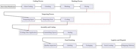
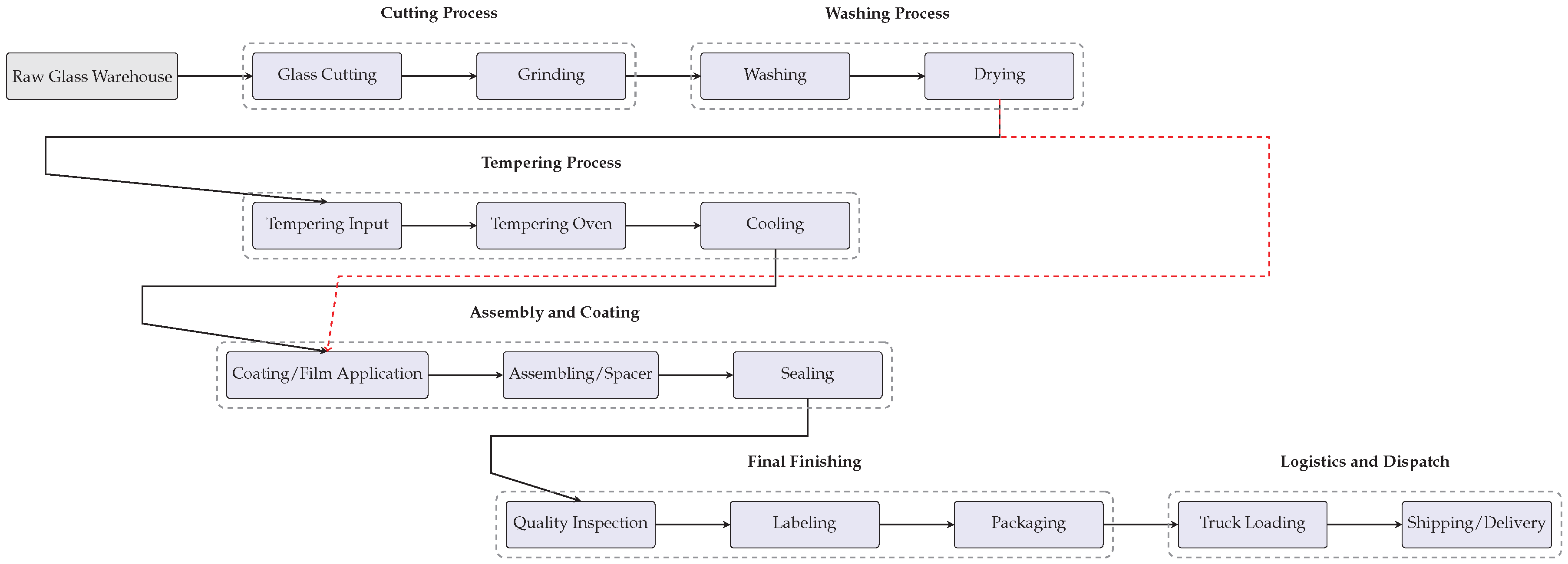
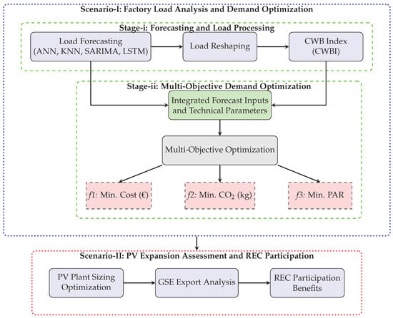
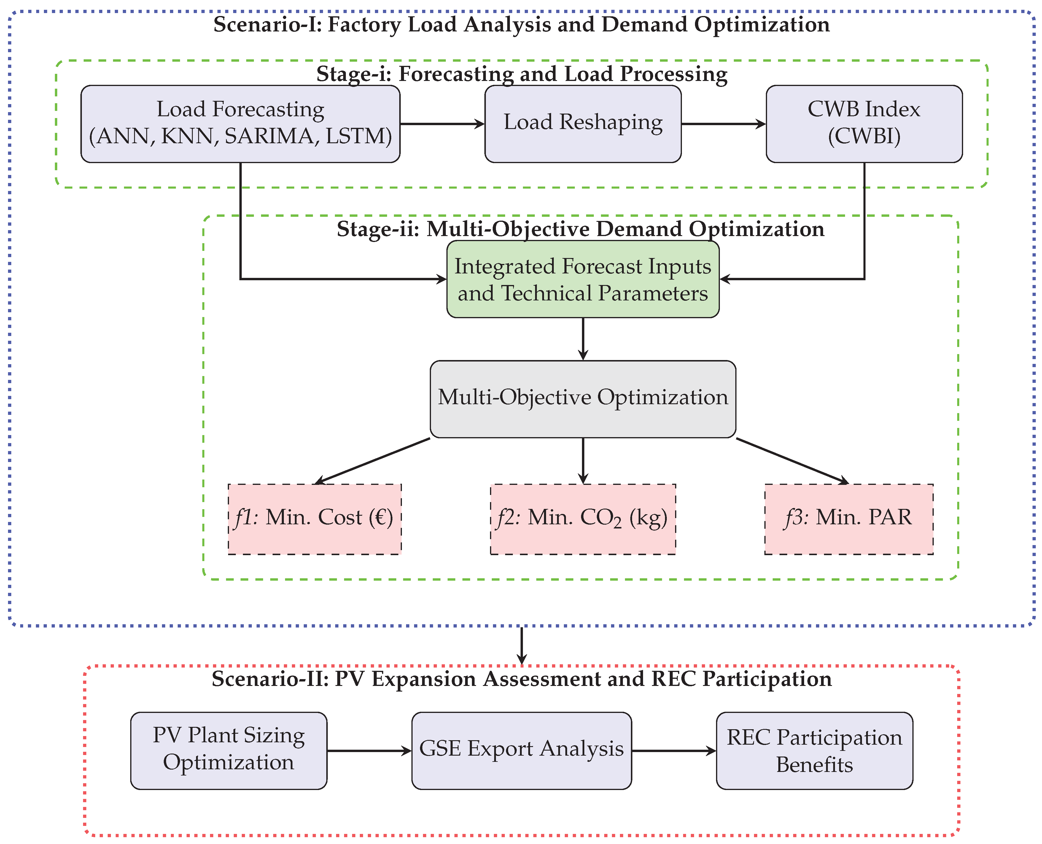
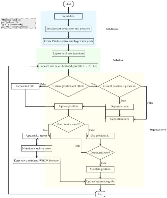
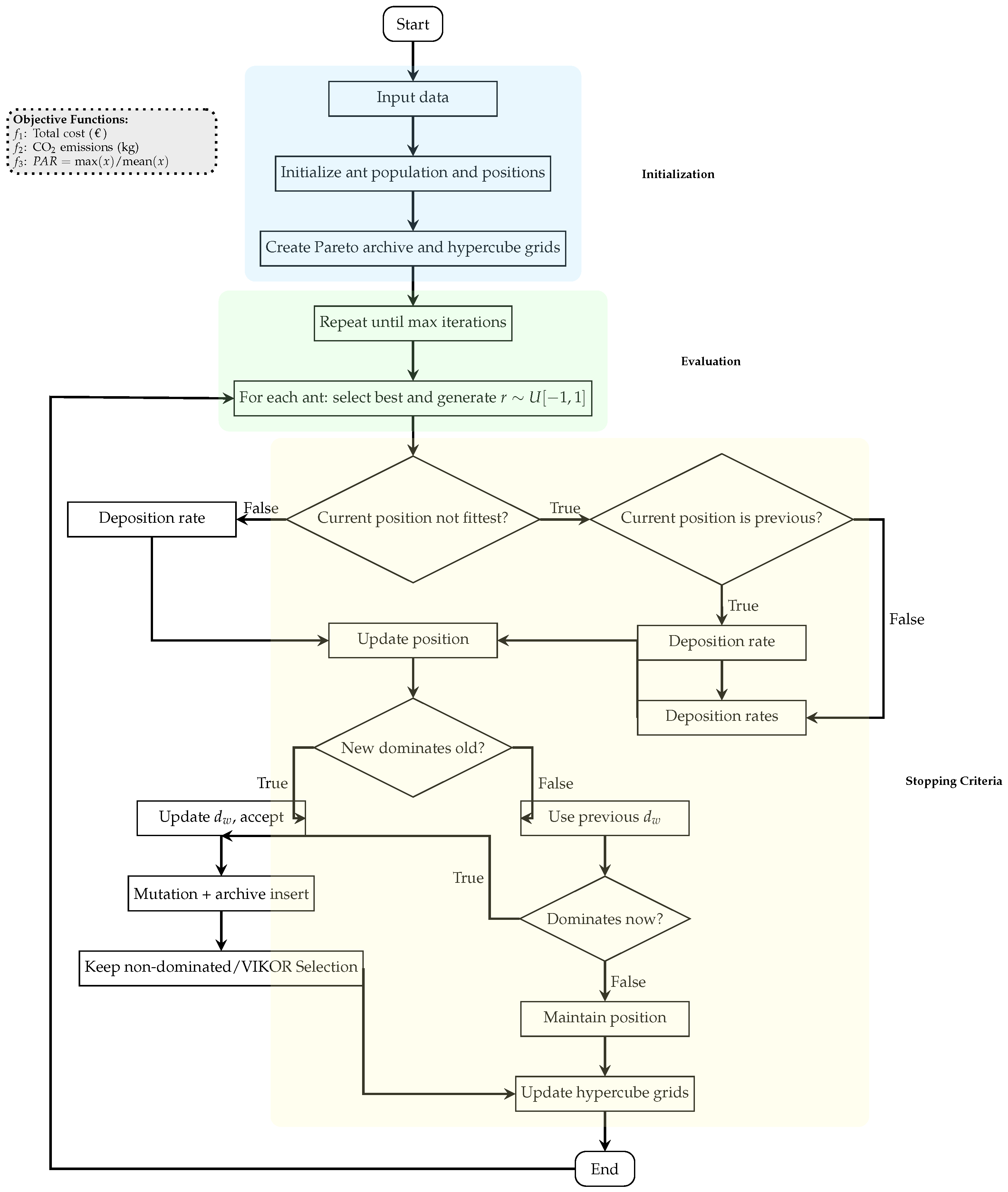
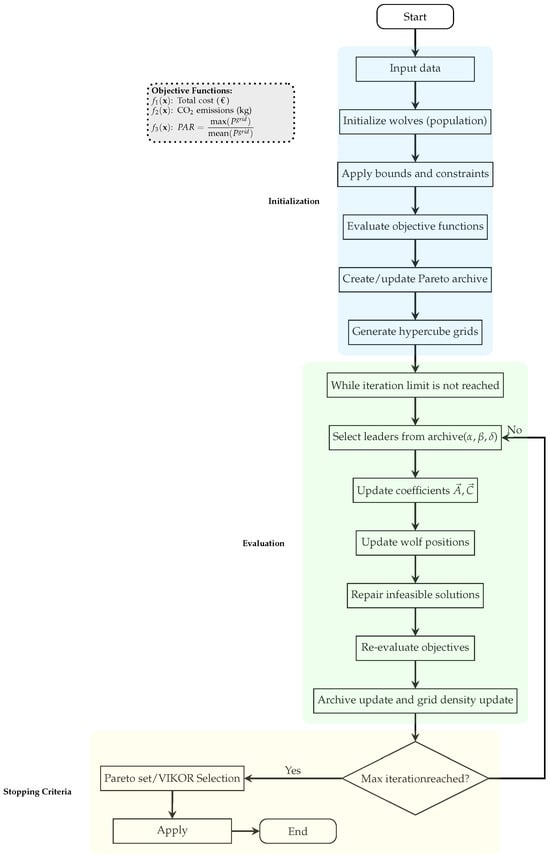
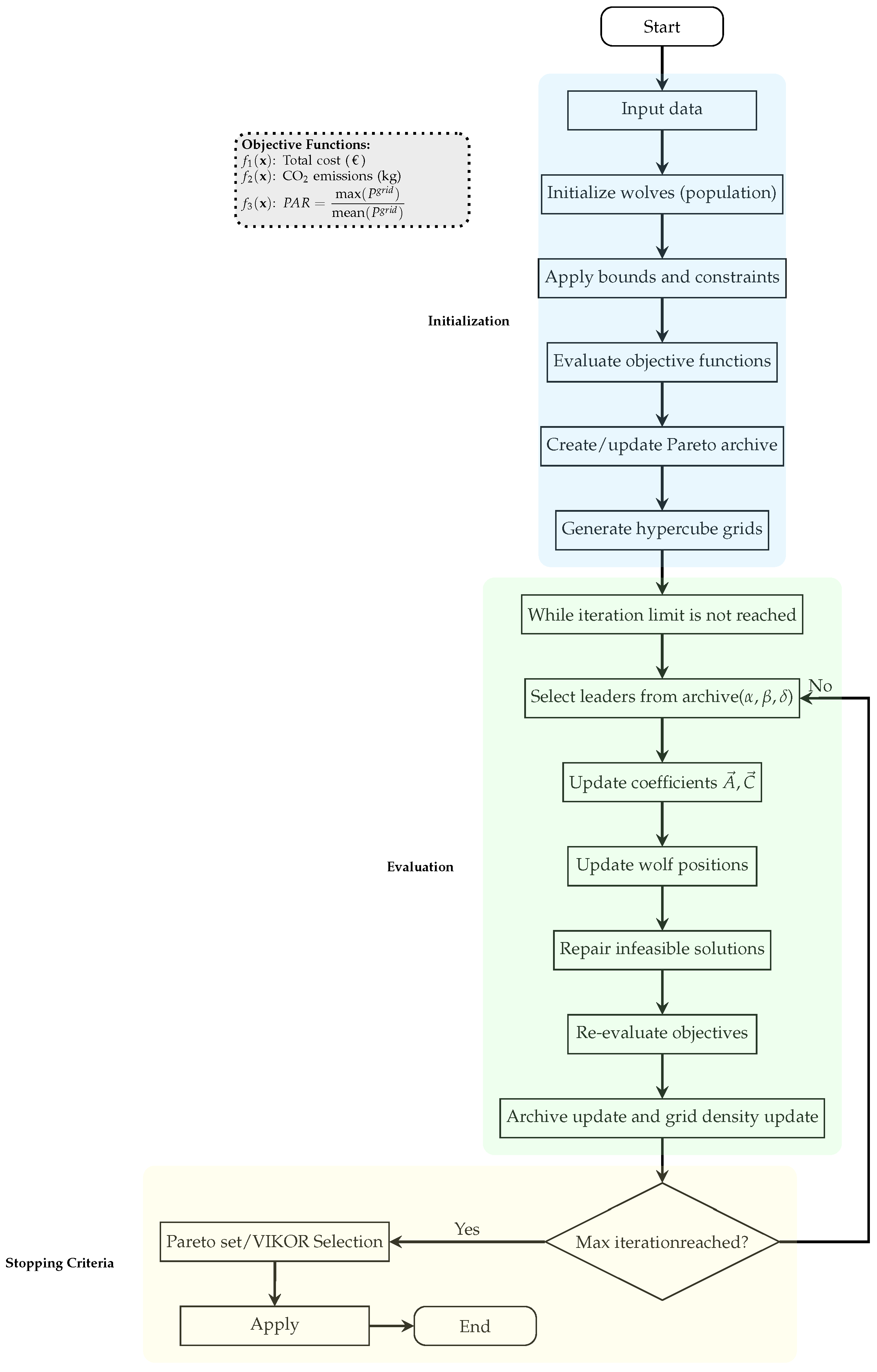
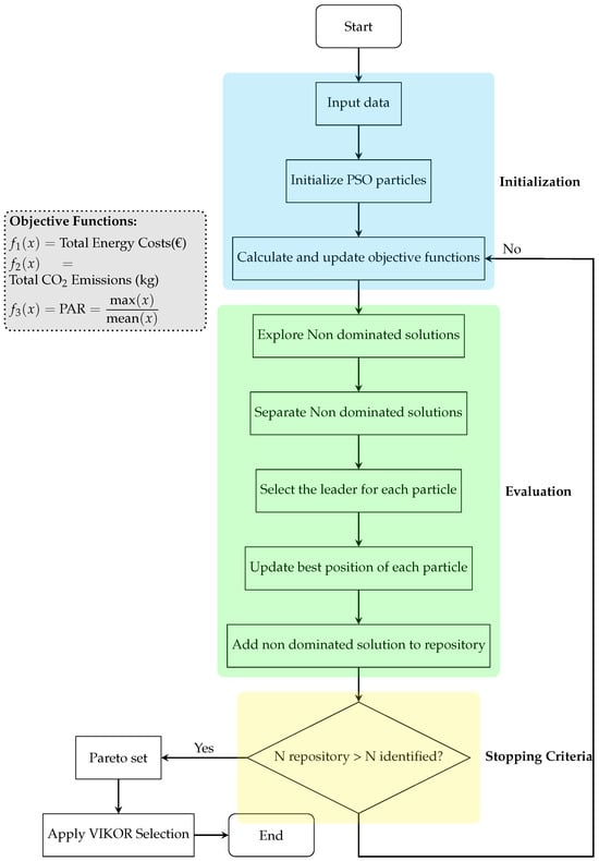
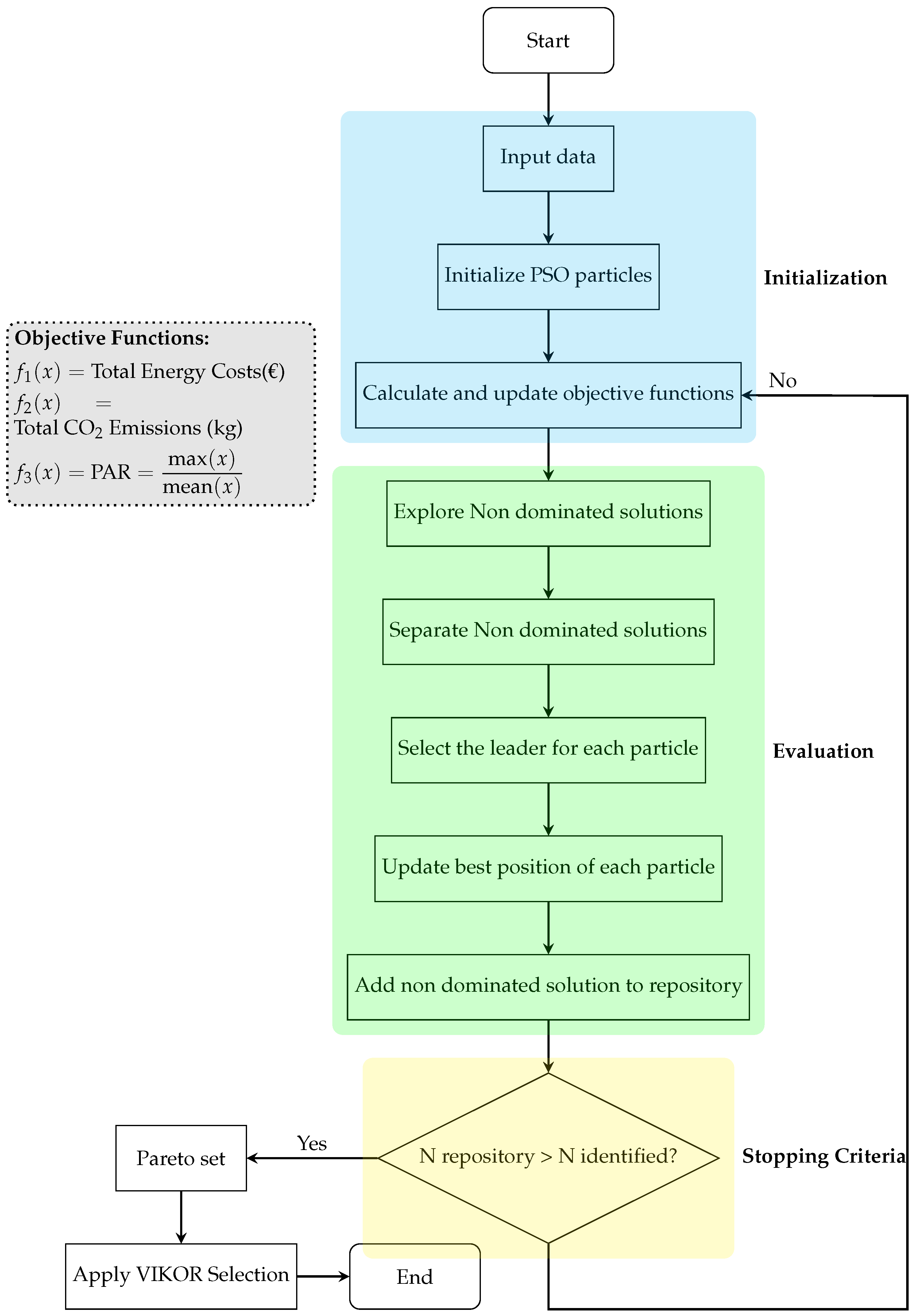
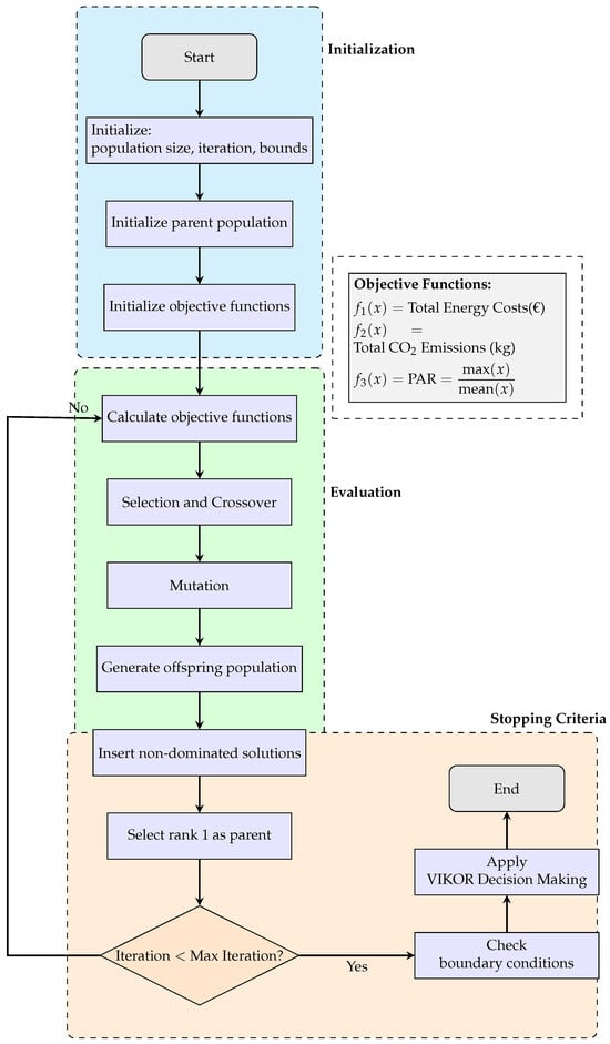
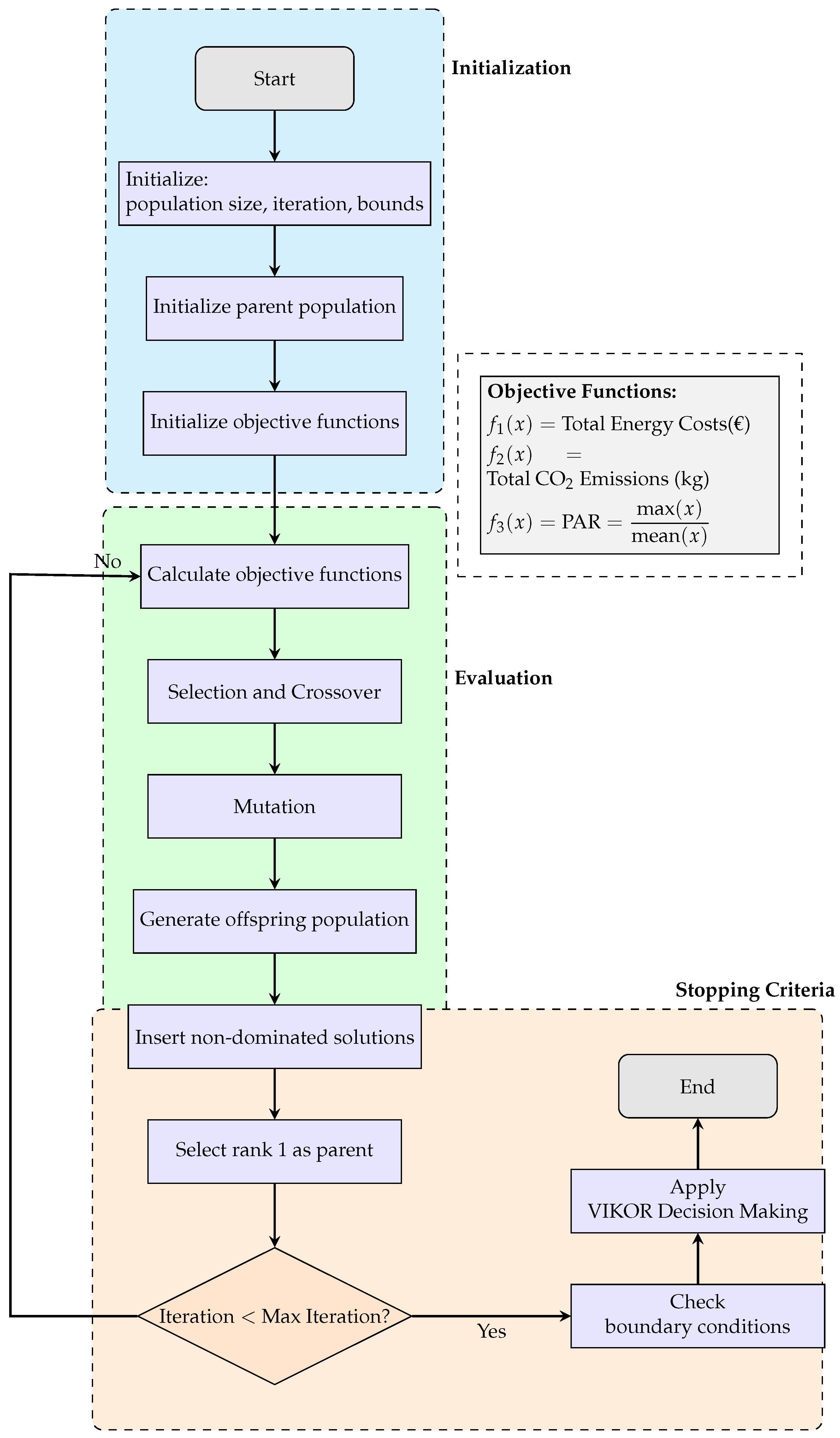
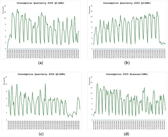
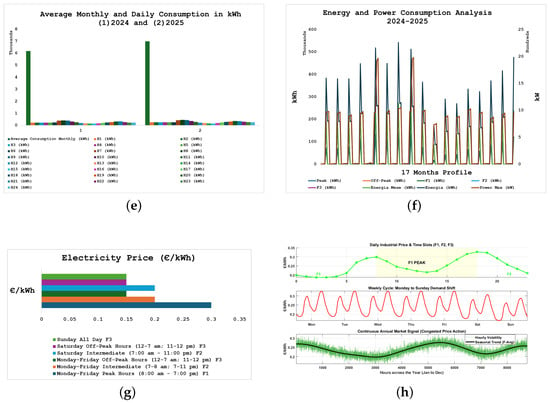
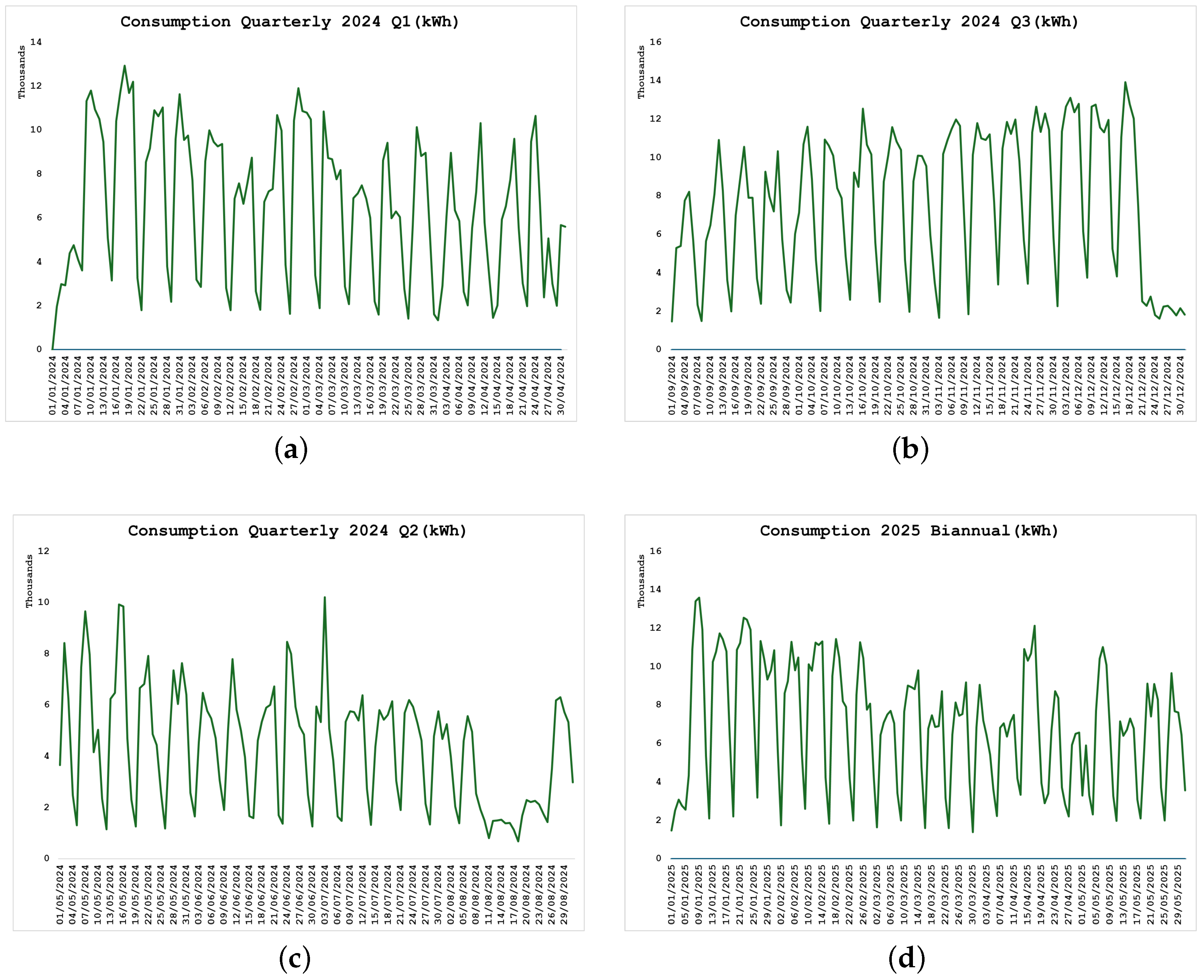
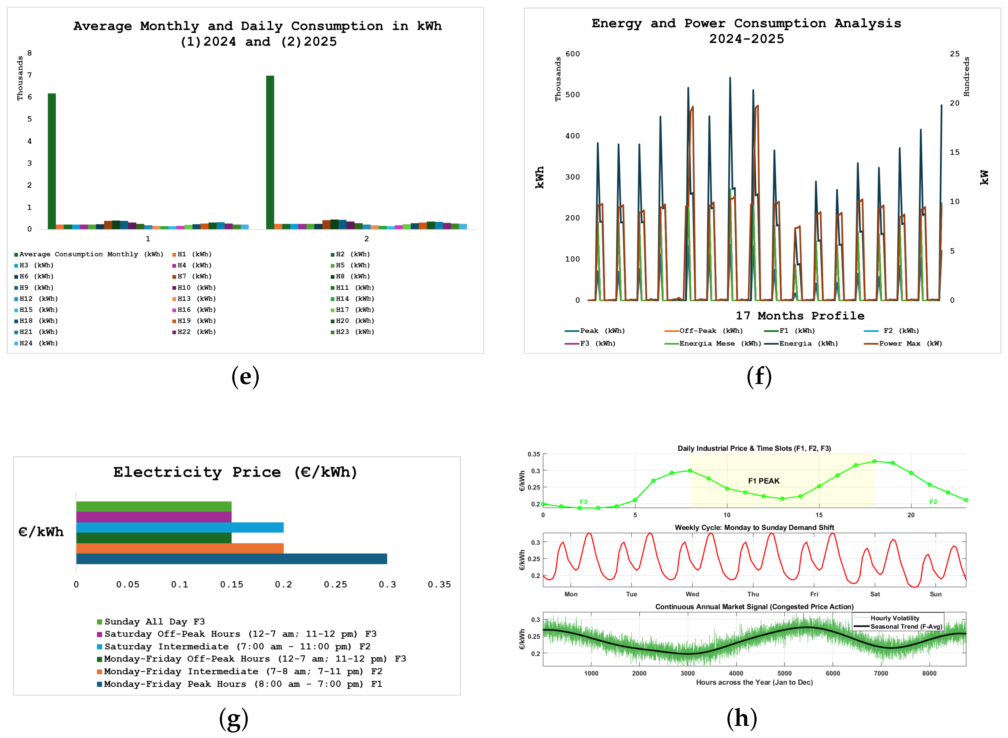
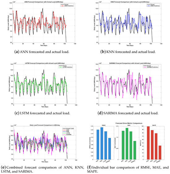
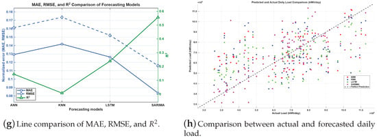
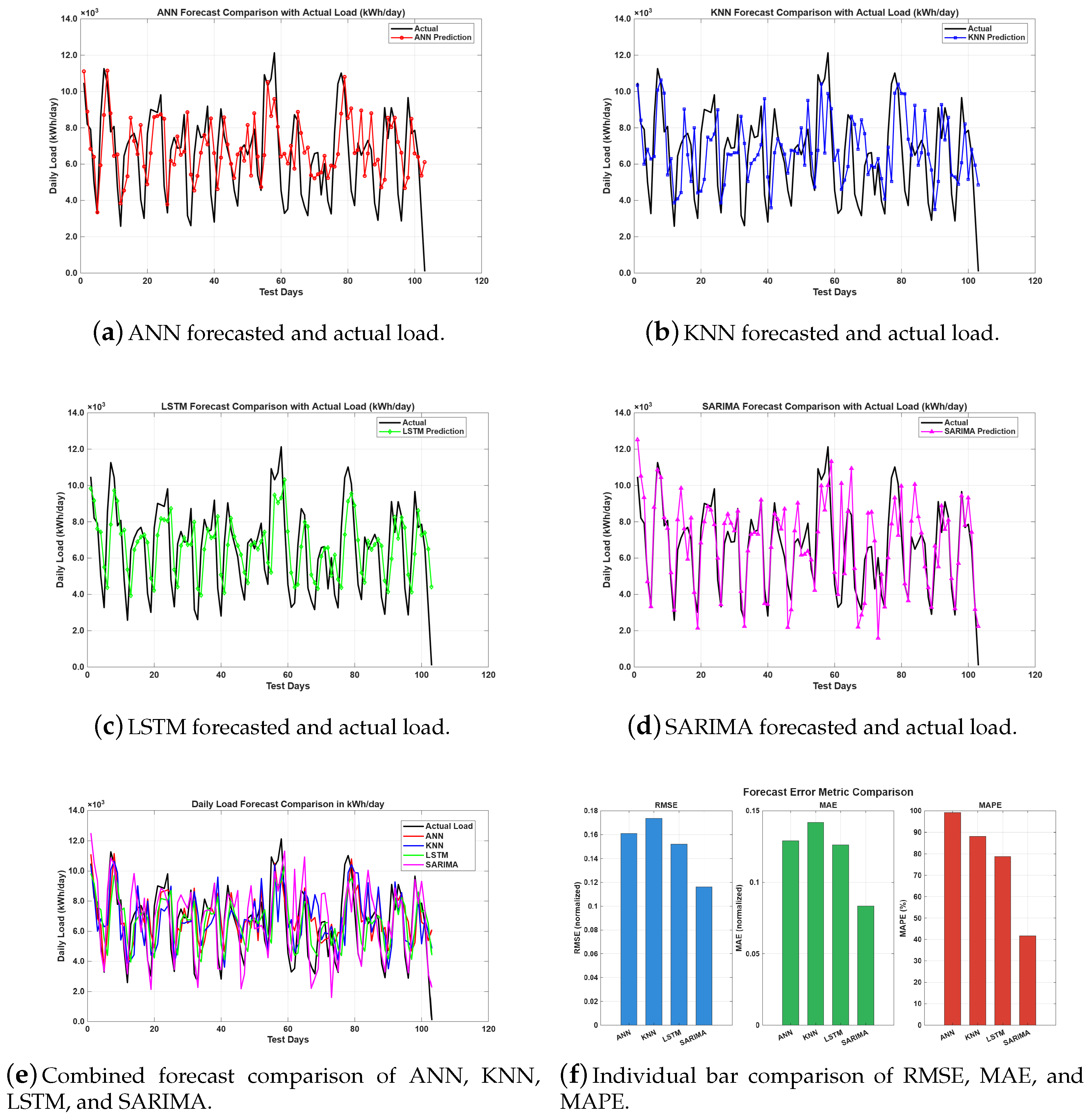
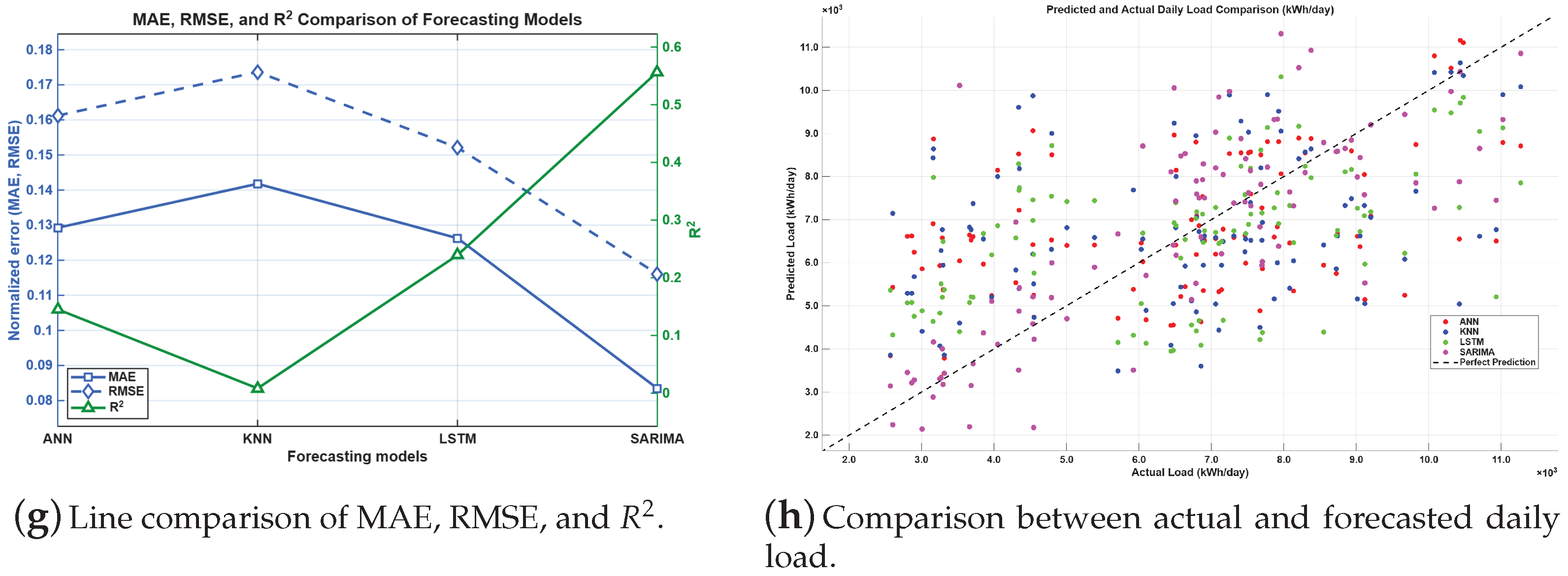
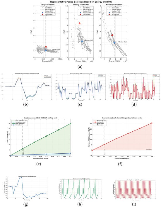
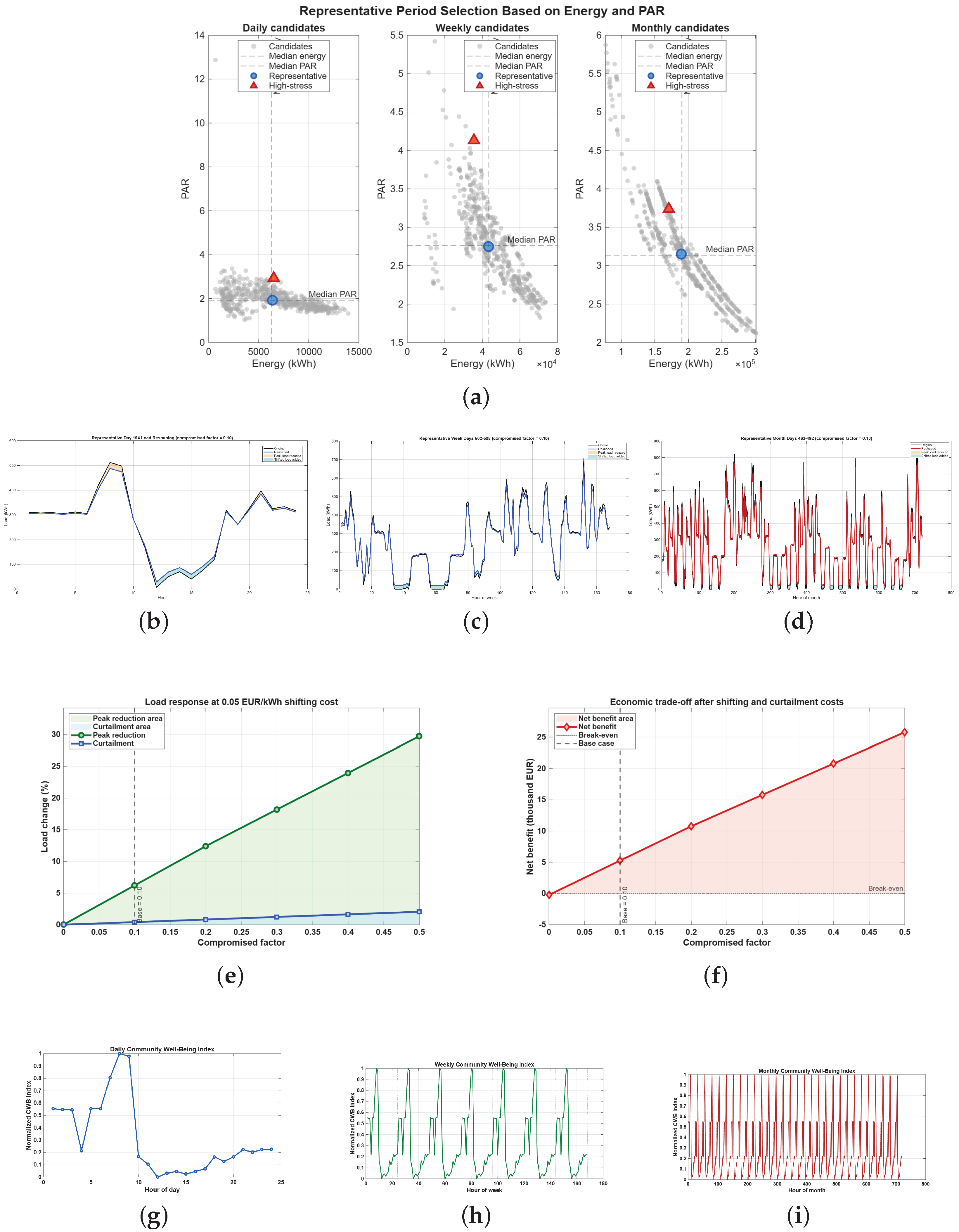
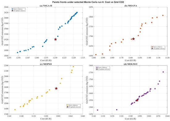
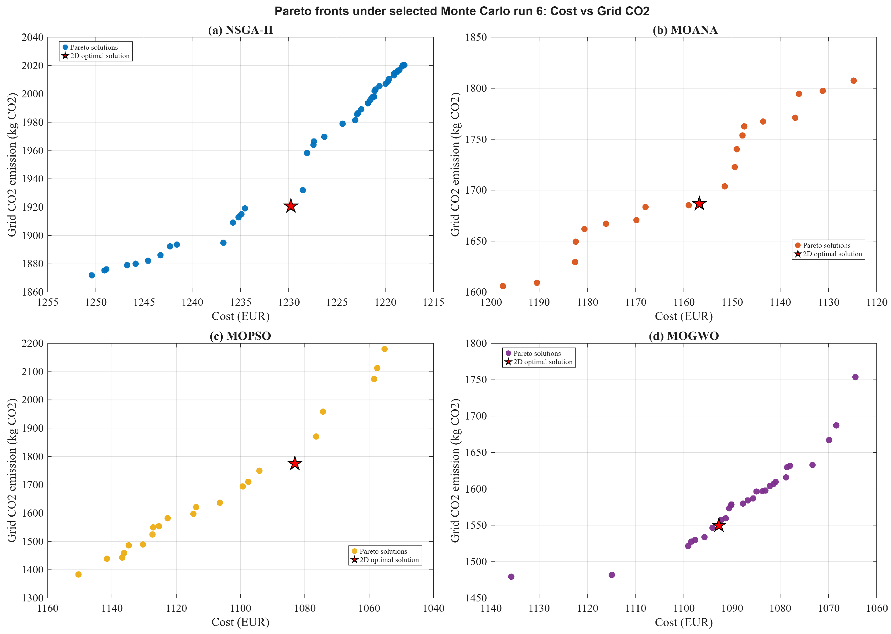
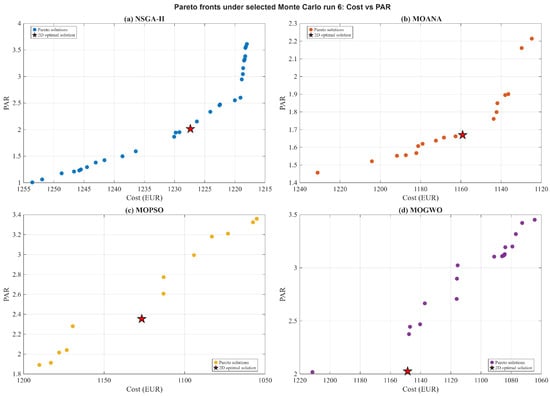
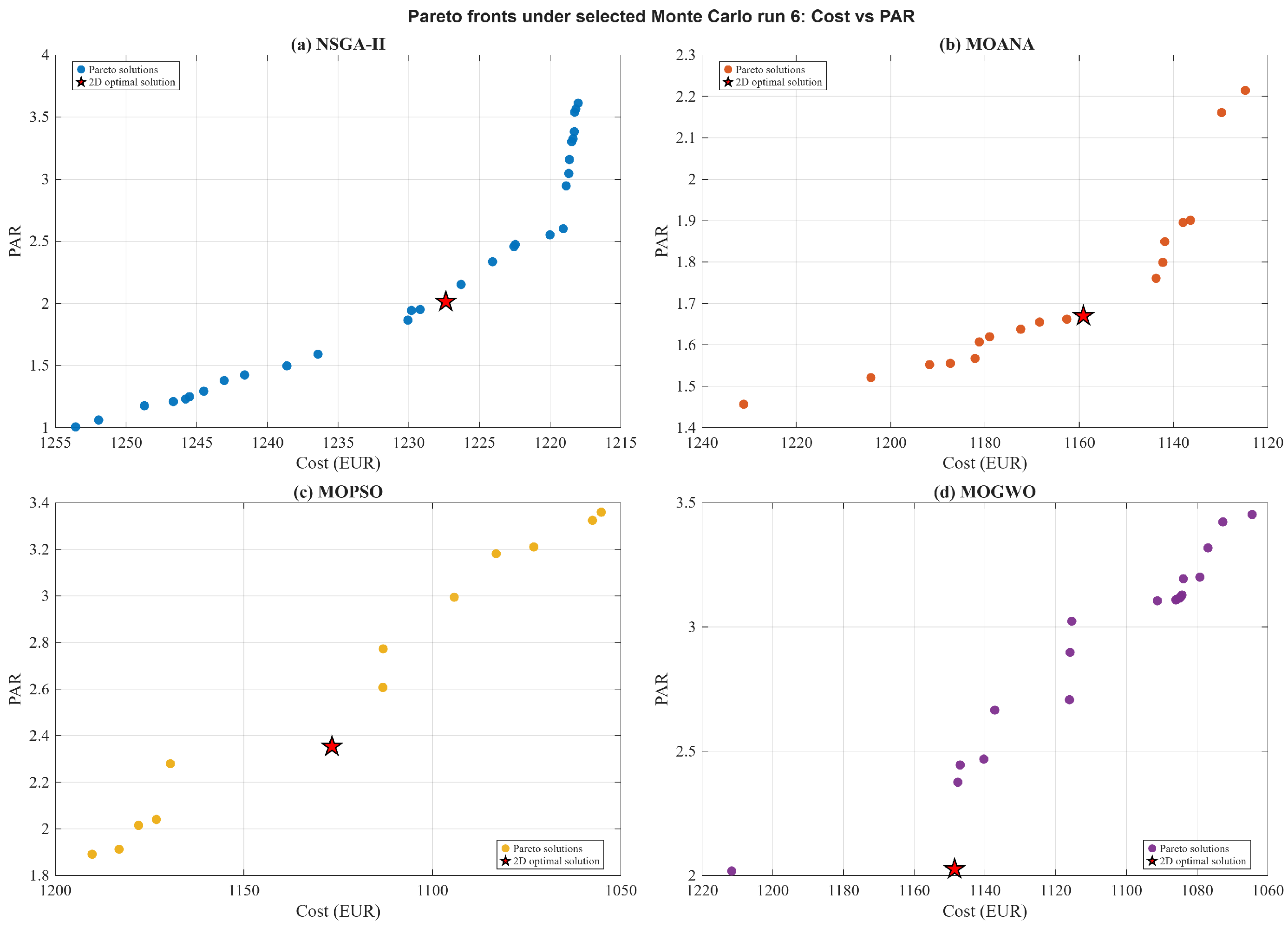
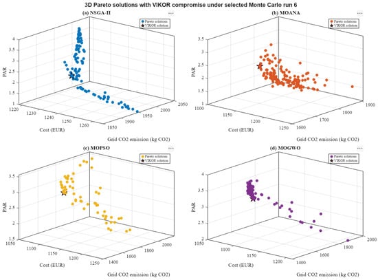
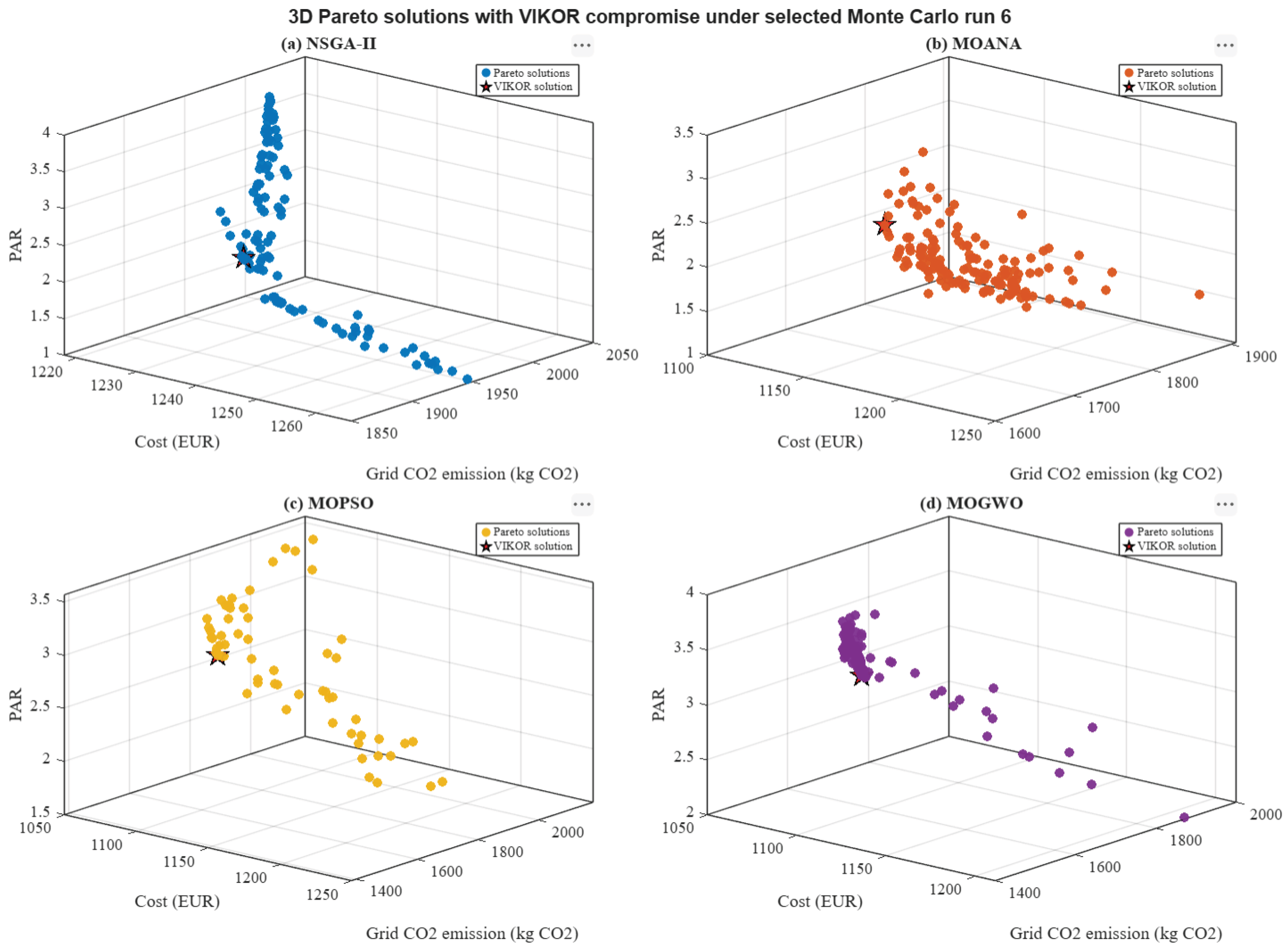
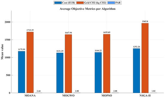
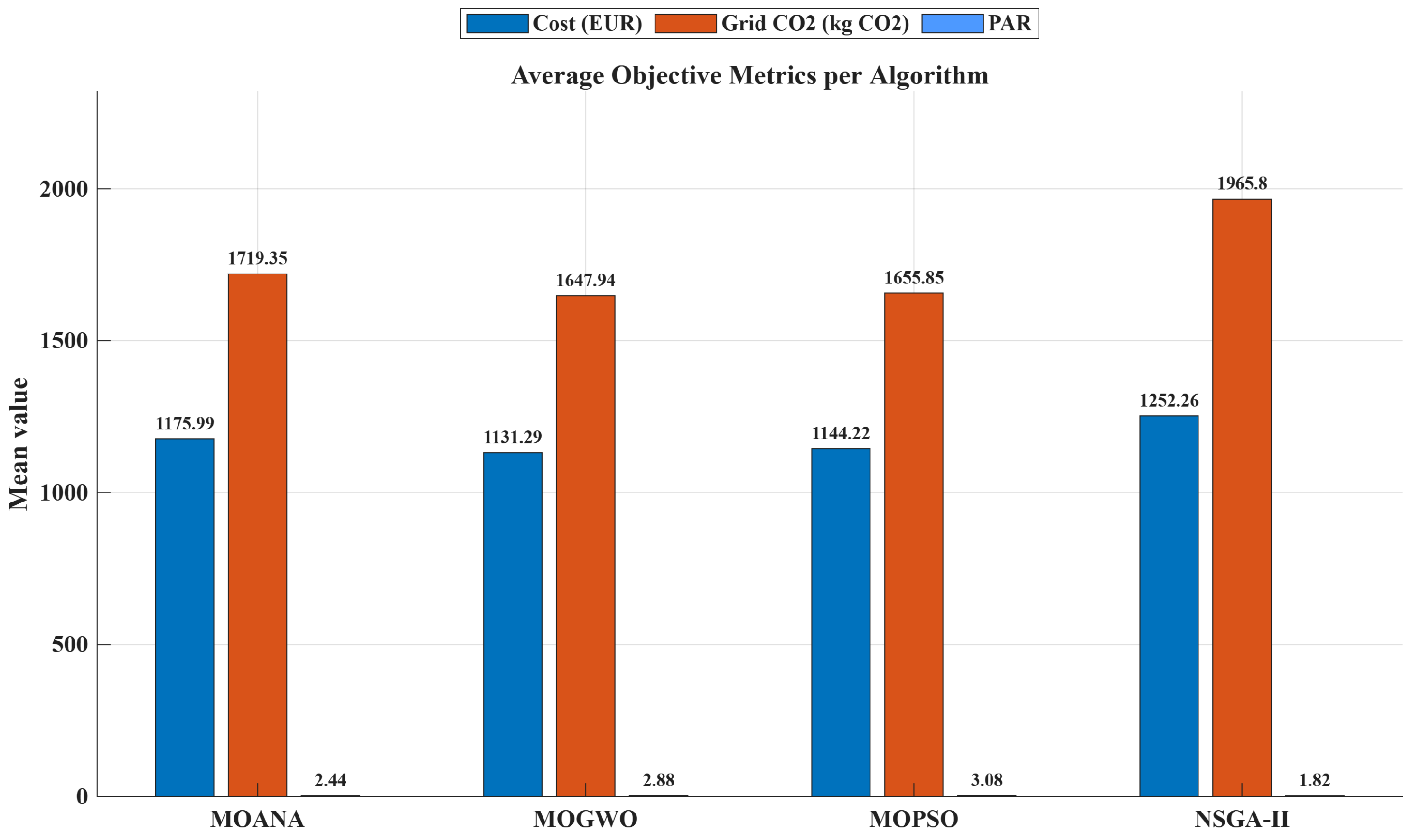
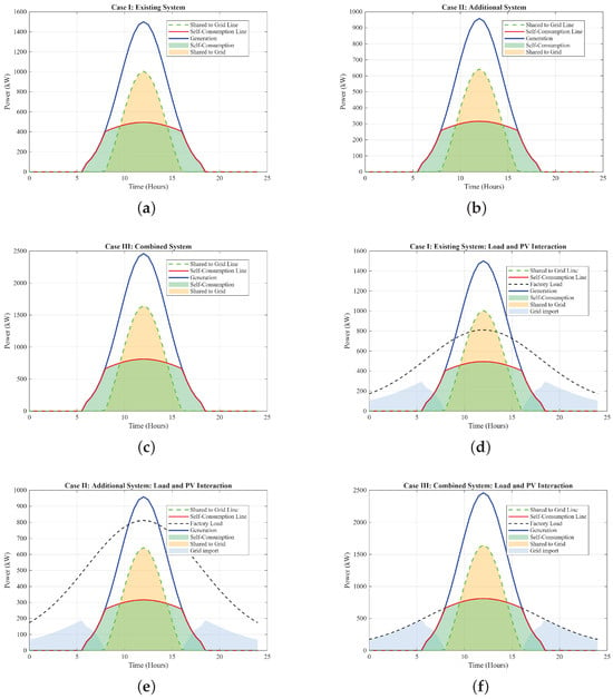
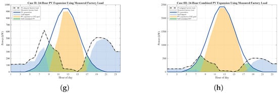
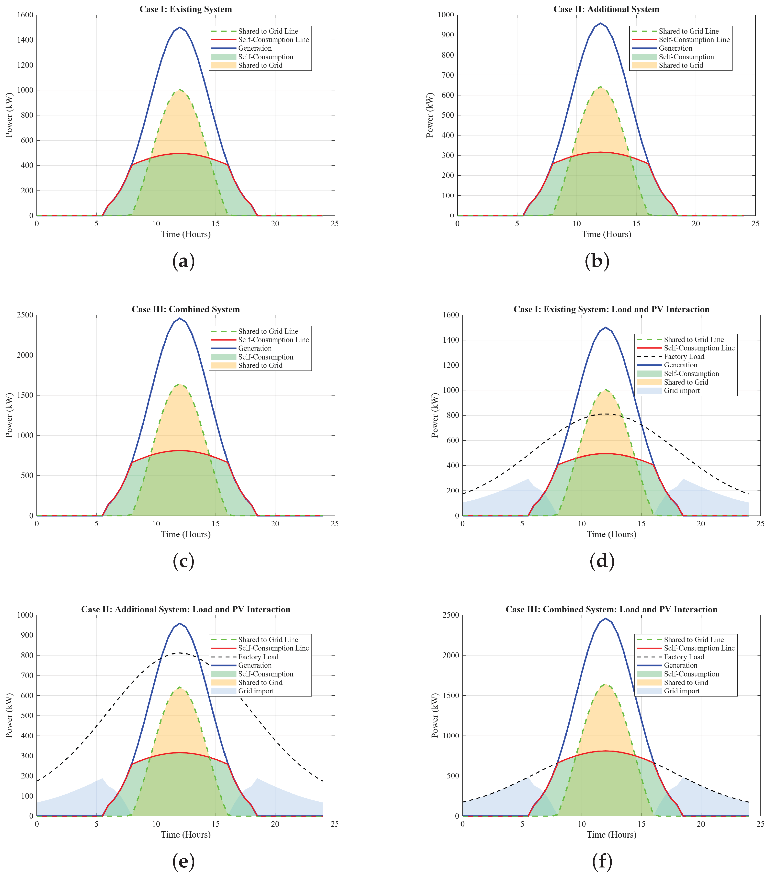
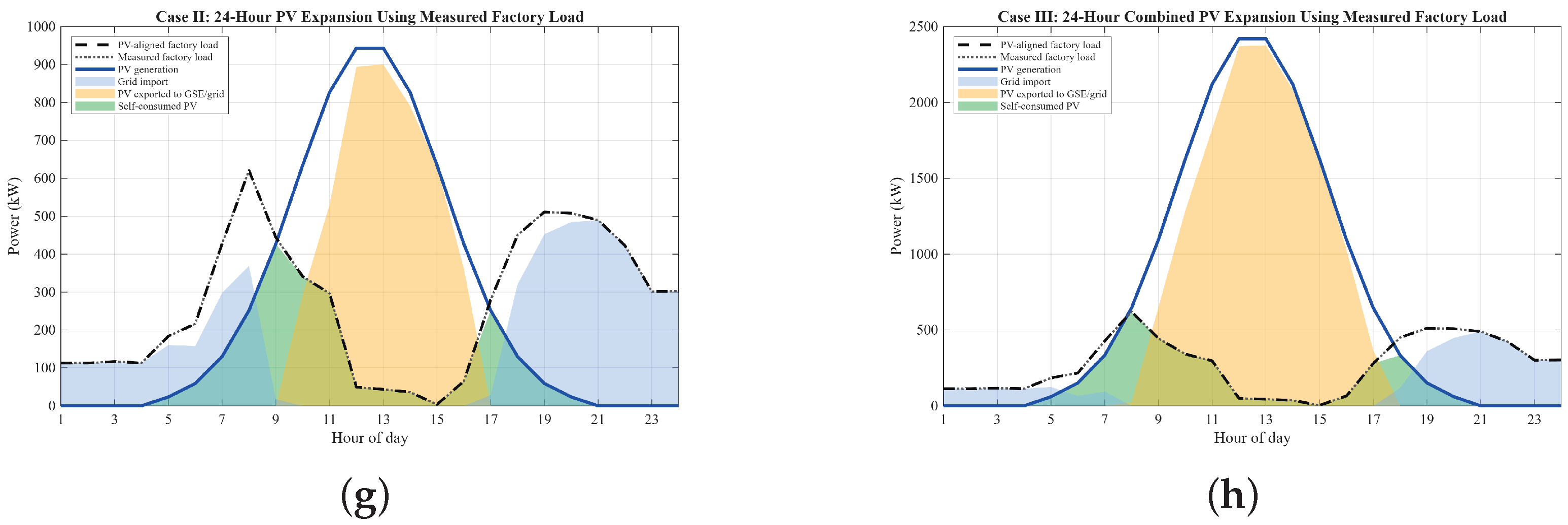
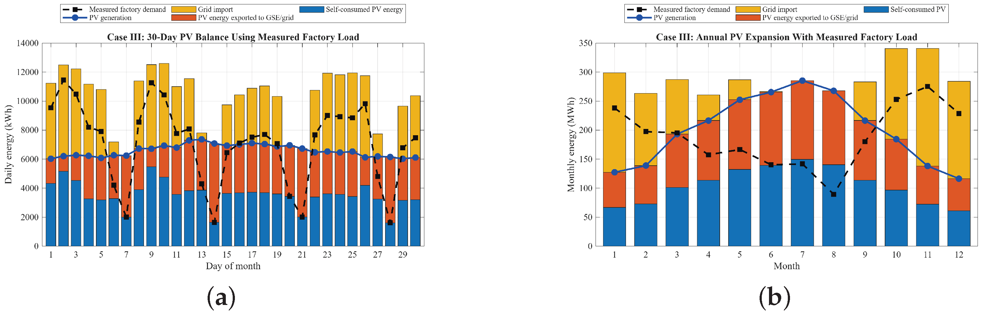

Disclaimer/Publisher’s Note: The statements, opinions and data contained in all publications are solely those of the individual author(s) and contributor(s) and not of MDPI and/or the editor(s). MDPI and/or the editor(s) disclaim responsibility for any injury to people or property resulting from any ideas, methods, instructions or products referred to in the content. |
© 2026 by the authors. Licensee MDPI, Basel, Switzerland. This article is an open access article distributed under the terms and conditions of the Creative Commons Attribution (CC BY) license.