Effect of Pressure Decline Rate on Horizontal Well Performance in Transitional Shale Gas Reservoirs

Abstract

Technical advances in horizontal drilling and hydraulic fracturing have been key drivers enabling the economic production of shale gas. While substantial efforts have been devoted to optimizing well productivity, the effect of the early pressure decline rate on horizontal well performance remains poorly understood in transitional shale gas reservoirs, which exhibit significant stress sensitivity. To address this, a multiscale flow model that integrates the Embedded Discrete Fracture Model (EDFM) with a geomechanical stress-sensitivity model was developed. This model describes the flow through matrix pores, bedding fractures, and hydraulic fractures and was validated against a field case. The results indicate that rapid fluid drainage during the early production stage creates a larger pressure drainage area. Specifically, a depletion rate of 0.2 MPa/d yields a 10% production increase over a rate of 0.05 MPa/d. However, stress sensitivity reduces overall production by approximately 20% while the bedding fracture connectivity can improve it by about 5%. For well X1H, the current production status suggests that gas and water are likely trapped or ‘blocked’ within the fractures; flow conductivity enhancement is recommended. For adjacent wells with a stress sensitivity coefficient exceeding 0.8, flow-restricted zones may extend into the matrix pores; stress sensitivity should be avoided.

1. Introduction

As the global energy structure shifts toward low-carbon and clean alternatives, shale gas has emerged as a critical unconventional natural gas resource and a key component of energy strategies [1]. China’s shale gas resources are primarily categorized into marine, marine–continental transitional, and continental facies [2,3]. In recent years, marine shale gas in formations such as the Longmaxi formation in the Sichuan basin has achieved large-scale commercial development, leading to a relatively mature theoretical and technological framework for exploration and production [4,5,6]. However, marine–continental transitional shale gas, which is widely distributed and accounts for approximately 25% of China’s total shale gas resources, exhibits significant exploration potential but has yet to achieve substantial breakthroughs, facing numerous development challenges [6,7,8].

Compared to marine shale, transitional shale exhibits distinct reservoir characteristics [2,9,10,11,12]. Typically, transitional shales feature thin individual layers (often <40–50 m), rapid lateral lithological variations, and relatively low brittle mineral contents (e.g., quartz and carbonate) but a predominance of Type III kerogen. Consequently, organic matter (OM) pores are poorly developed. The reservoir space is instead dominated by clay mineral-associated pores, such as interlaminar and intergranular pores, as well as microfractures. These attributes contribute to a generally lower gas-bearing capacity than marine shales, with the measured gas content often significantly below theoretical predictions. Shale gas in transitional reservoirs occurs predominantly as adsorbed gas, with a relatively low proportion of free gas. Furthermore, transitional shales are frequently interbedded with coal seams and tight sandstones, forming a layered “sandwich”-like lithological configuration. This structure enhances hydrocarbon expulsion efficiency, allowing a significant portion of generated gas to migrate into adjacent sandstone layers, thereby further reducing the free gas content retained within the shale itself.

The flow characteristics also differ significantly. Marine shale gas is predominantly free gas, characterized by higher reservoir permeability and simpler flow mechanisms dominated by transition flow and Knudsen diffusion [13,14,15]. In contrast, marine–continental transitional shale gas exhibits more complex flow behavior due to its high clay mineral content (averaging 48.29%) and elevated water saturation. These conditions restrict effective flow pathways, enhance water-blocking effects, and result in multiscale flow with multi-flow regimes, where transition flow is often dominant. The flow regimes around hydraulic fractures in such reservoirs include linear, bilinear, elliptical, and pseudo-radial flow. Among these, elliptical flow persists for an extended duration in low-permeability reservoirs and is a critical phase for predicting reservoir properties and fracture parameters.

Reservoir modeling of transitional shale is particularly challenging due to the pronounced heterogeneity and complex multiscale fracture systems, which impede conventional methods from accurately characterizing storage space and flow networks [16,17,18]. These reservoirs exhibit strong vertical heterogeneity in organic matter content and mineral composition. The pore system is dominated by inorganic pores (intergranular and intracrystalline), while organic matter pores are poorly developed. The pore morphology is primarily characterized by parallel plate-like fissures, often accompanied by ink-bottle-type pores formed by the combination of micro- and macropores, further complicating the pore structure. Furthermore, the fracture systems are multiscale, multi-genetic, and developed over multiple phases. These systems comprise a combination of tectonic fractures (tensile, shear, and squeeze) and non-tectonic fractures (e.g., dissolution fractures), controlled by factors such as tectonic position, proximity to faults, rock brittleness, single-sand-body thickness, and diagenesis. The spatial distribution of these fractures is often highly disordered. Critically, in areas with strong reflection shielding from interbedded coal seams, conventional post-stack seismic attributes fail to effectively detect fracture discontinuities, leading to significant inaccuracies in models reliant on single-attribute analysis.

Furthermore, transitional shale reservoirs generally exhibit strong stress sensitivity [19,20,21]. During production, declining reservoir pressure increases effective stress, leading to fracture closure and a sharp reduction in permeability, severely impairing productivity. Previous studies have shown that the stress sensitivity coefficient of shale reservoirs typically ranges from 0.1 to 1.6 MPa⁻¹, with permeability damage rates reaching 61.44–73.93% (averaging about 69.92%), confirming a high degree of stress sensitivity [20]. Research based on dual-porosity models further reveals that stress sensitivity is closely related to the shale pore structure: when the ratio of matrix porosity to microfracture porosity is low, the porosity sensitivity exponent decreases while pore compressibility increases, resulting in more pronounced stress-dependent behavior. In addition, the presence of tortuosity also enhances stress sensitivity, further exacerbating permeability loss. Multiscale flow simulations demonstrate that stress sensitivity can reduce productivity by approximately 20%. Under highly stress-sensitive conditions, flow-restricted zones may extend into the matrix, further accelerating production decline. Therefore, accurate evaluation of shale stress sensitivity and its controlling factors is essential for reliable productivity prediction and optimized development strategies.

Therefore, efficient development of transitional shale gas cannot rely solely on experience from marine shale but requires targeted research into production strategy optimization based on its unique geological and engineering characteristics. A critical aspect is liquid drainage strategy, where the initial water drainage rate significantly impacts the pressure drainage area and ultimate recovery. While rapid drainage helps expand the pressure drainage region, it must be compatible with the reservoir’s stress-sensitive characteristics to avoid irreversible damage from excessive pressure drawdown, such as fracture closure and permeability impairment.

In summary, the effective development of marine–continental transitional shale gas urgently requires systematic research into reservoir characterization, flow mechanisms, stress sensitivity, and production optimization. This study utilizes multiscale modeling and numerical simulation to reveal the mechanisms by which initial permeability, stress sensitivity and pressure depletion impact the productivity of horizontal wells. The aim is to provide a theoretical basis and technical support for the efficient development of transitional shale gas.

2. Mathematical Modeling

2.1. Assumptions

Based on previous studies characterizing the pore structure and fluid transport mechanisms in transitional shale gas reservoirs [9,10,11,12,13,14,15], the following foundational assumptions are adopted in this study:

(1) The shale formation is represented as a dual-porosity system composed of matrix pores and bedding fractures, both of which contribute to permeability.

(2) The shale rock framework, including the matrix pores and bedding fractures, is compressible, resulting in stress-sensitive behavior under varying effective stress.

(3) Within nanoscale matrix pores, the capillary force is the dominant driving mechanism.

(4) Within microscale fractures and fracture networks, the relevant driving mechanisms are the pressure difference, gravity, and capillary force.

(5) Within the wellbore, flow is driven primarily by the pressure gradient and gravity.

(6) Shale gas and water are assumed immiscible since the molar fraction of methane in water at 40 MPa is only 0.01 [22].

2.2. Governing Equation

2.2.1. Hydraulic Fractures

The migration of gas and water within the hydraulic fracture networks is governed by Equations (1) and (2).

$$\mathsf{\nabla }\left[{\displaystyle \frac{k_F{k}_{Frg}}{{\mu }_{Fg}{B}_{Fg}}}\mathsf{\nabla }\left(p_{Fg}-{\rho }_{Fg}gH\right)\right]+q_{fFg}-q_{gwell}={\displaystyle \frac{\mathsf{\partial }}{\mathsf{\partial }t}}\left({\displaystyle \frac{{{\varphi }_{F}S}_{Fg}}{B_{Fg}}}\right)$$

(1)

$$\mathsf{\nabla }\left[{\displaystyle \frac{k_F{k}_{Frw}}{{\mu }_{Fw}{B}_{Fw}}}\mathsf{\nabla }\left(p_{Fw}-{\rho }_{Fw}gH\right)\right]+q_{fFw}-q_{wwell}={\displaystyle \frac{\mathsf{\partial }}{\mathsf{\partial }t}}\left({\displaystyle \frac{{{\varphi }_{F}S}_{Fw}}{B_{Fw}}}\right)$$

(2)

where $k_F$ represents the permeability for hydraulic fracture, mD; $k_{Frg}$ is the relative permeability of gas flow in hydraulic fracture, dimensionless; ${\mu }_{Fg}$ is the gas viscosity in hydraulic fracture, Pa·s; $B_{Fg}$ is the formation volume factor of gas in hydraulic fracture, m³/m³; $p_{Fg}$ is the gas pressure in hydraulic fracture, MPa; ${\rho }_{Fg}$ is the gas density in hydraulic fracture, kg/m³; $q_{fFg}$ is the gas crossflow rate between bedding fracture and hydraulic fracture, m³/(m³·d); $q_{gwell}$ is the gas production rate, m³/(m³·d); ${\varphi }_F$ is the porosity for hydraulic fracture, dimensionless; $s_{Fg}$ is the gas saturation in hydraulic fracture, dimensionless; $k_{Frw}$ is the relative permeability of water flow in hydraulic fracture, dimensionless; ${\mu }_{Fw}$ is the water viscosity in hydraulic fracture, Pa·s; $B_{Fw}$ is the formation volume factor of water in hydraulic fracture, m³/m³; $p_{Fw}$ is the water pressure in hydraulic fracture, MPa; ${\rho }_{Fw}$ is the water density in hydraulic fracture, kg/m³; $q_{Ffw}$ is the water crossflow rate between bedding fracture and hydraulic fracture, m³/(m³·d); $q_{wwell}$ is the water production rate, m³/(m³·d); and $s_{Fw}$ is the water saturation in hydraulic fracture, dimensionless.

2.2.2. Bedding Fractures

For the bedding fractures within the shale, gas and water migration follows Equations (3) and (4).

$$\mathsf{\nabla }\left[{\displaystyle \frac{k_f{k}_{frg}}{{\mu }_{fg}{B}_{fg}}}\mathsf{\nabla }\left(p_{fg}-{\rho }_{fg}gH\right)\right]+q_{mfg}-q_{fFg}={\displaystyle \frac{\mathsf{\partial }}{\mathsf{\partial }t}}\left({\displaystyle \frac{{{\varphi }_{f}S}_{fg}}{B_{fg}}}\right)$$

(3)

$$\mathsf{\nabla }\left[{\displaystyle \frac{k_f{k}_{frw}}{{\mu }_{fw}{B}_{fw}}}\mathsf{\nabla }\left(p_{fw}-{\rho }_{fw}gH\right)\right]-q_{fFw}={\displaystyle \frac{\mathsf{\partial }}{\mathsf{\partial }t}}\left({\displaystyle \frac{{{\varphi }_{f}S}_{fw}}{B_{fw}}}\right)$$

(4)

where $k_f$ represents the permeability for bedding fracture, mD; $k_{frg}$ is the relative permeability of gas flow in bedding fracture, dimensionless; ${\mu }_{fg}$ is the gas viscosity in bedding fracture, Pa·s; $B_{fg}$ is the formation volume factor of gas in bedding fracture, m³/m³; $p_{fg}$ is the gas pressure in bedding fracture, MPa; ${\rho }_{fg}$ is the gas density in bedding fracture, kg/m³; $q_{mfg}$ is the gas crossflow rate between matrix pore and bedding fracture, m³/(m³·d); ${\varphi }_f$ is the porosity for bedding fracture, dimensionless; $s_{fg}$ is the gas saturation in bedding fracture, dimensionless; $k_{frw}$ is the relative permeability of water flow in bedding fracture, dimensionless; ${\mu }_{fw}$ is the water viscosity in bedding fracture, Pa·s; $B_{fw}$ is the formation volume factor of water in bedding fracture, m³/m³; $p_{fw}$ is the water pressure in bedding fracture, MPa; ${\rho }_{fw}$ is the water density in bedding fracture, kg/m³; and $s_{fw}$ is the water saturation in bedding fracture, dimensionless.

2.2.3. Matrix Pores

Within the matrix pores, the migration of gas and water are described by Equations (5) and (6).

$$\mathsf{\nabla }\left[{\displaystyle \frac{k_m{k}_{mrg}}{{\mu }_{mg}{B}_{mg}}}\mathsf{\nabla }\left(p_{mg}-{\rho }_{mg}gH\right)\right]-q_{mfg}={\displaystyle \frac{\mathsf{\partial }}{\mathsf{\partial }t}}\left({\displaystyle \frac{{{\varphi }_{m}S}_{mg}}{B_{mg}}}\right)$$

(5)

$$\mathsf{\nabla }\left[{\displaystyle \frac{k_m{k}_{mrw}}{{\mu }_{mw}{B}_{mw}}}\mathsf{\nabla }\left(p_{mw}-{\rho }_{mw}gH\right)\right]={\displaystyle \frac{\mathsf{\partial }}{\mathsf{\partial }t}}\left({\displaystyle \frac{{{\varphi }_{m}S}_{mw}}{B_{mw}}}\right)$$

(6)

where $k_m$ represents the permeability for matrix pores, mD; $k_{mrg}$ is the relative permeability of gas flow in matrix pores, dimensionless; ${\mu }_{mg}$ is the gas viscosity in matrix pores, Pa·s; $B_{mg}$ is the formation volume factor of gas in matrix pores, m³/m³; $p_{mg}$ is the gas pressure in matrix pores, MPa; ${\rho }_{mg}$ is the gas density in matrix pores, kg/m³; ${\varphi }_m$ is the porosity for matrix pores, dimensionless; $s_{mg}$ is the gas saturation in matrix pores, dimensionless; $k_{mrw}$ is the relative permeability of water flow in matrix pores, dimensionless; ${\mu }_{mw}$ is the water viscosity in matrix pores, Pa·s; $B_{mw}$ is the formation volume factor of water in matrix pores, m³/m³; $p_{mw}$ is the water pressure in matrix pores, MPa; ${\rho }_{mw}$ is the water density in matrix pores, kg/m³; and $s_{mw}$ is the water saturation in matrix pores, dimensionless.

2.2.4. Crossflow

The transfer of gas and water between the bedding fractures and the hydraulic fractures is represented by the crossflow terms in Equations (7) and (8).

$$q_{fFg}=D{F}_s\left({\displaystyle \frac{1}{L_x^2}}+{\displaystyle \frac{1}{L_y^2}}+{\displaystyle \frac{1}{L_z^2}}\right)\left({\displaystyle \frac{s_{fg}}{B_{fg}}}-{\displaystyle \frac{s_{Fg}}{B_{Fg}}}\right)$$

(7)

$$q_{fFw}={\alpha }_s{\displaystyle \frac{k_f{k}_{frw}}{{\mu }_{fw}{B}_{fw}}}\left[\left(p_{fw}-{\rho }_{fw}gH\right)-\left(p_{Fw}-{\rho }_{Fw}gH\right)\right]$$

(8)

where $D$ is the diffusion coefficient of gas, m²/s; $F_s$ is the pore shape factor, dimensionless; $L_x$, $L_y$, and $L_z$ are bedding fracture spacing in x, y, and z directions, respectively, m; and ${\alpha }_s$ is the Gilman and Kazemi shape factor, dimensionless.

2.2.5. Gas Desorption

Beyond advective flow, the desorption of methane from organic-rich shale matrices involves multiscale transport phenomena governed by concentration gradients and pore-structure effects. Unlike conventional reservoirs, shale exhibits unique desorption characteristics due to its nanoporous architecture and organic matter distribution. Methane molecules adsorbed on pore surfaces undergo diffusion through the organic matrix. This process is modeled using a modified Fickian model that incorporates Knudsen diffusion and surface diffusion components:

$$q_{mfg}={\displaystyle \frac{\mathsf{\partial }{V}_m}{\mathsf{\partial }t}}$$

(9)

where

$$V_m={\displaystyle \frac{V_{L}p}{p+p_L}}$$

(10)

where $V_m$ represents the gas adsorption within the matrix pore, m³/m³.

2.3. Stress Sensitivity

Furthermore, shale exhibits significant stress sensitivity, meaning that shale porosity and permeability vary with effective stress [23,24,25]. The evolution of porosity and permeability in the bedding fractures during production is described by the following relationship:

$${\varphi }_f={\varphi }_{fi}{e}^{-C_{\mathrm{f}}{\Delta \sigma }_e^h}$$

(11)

$$k_f=k_{fi}{e}^{-3C_{\mathrm{f}}{\Delta \sigma }_e^h}$$

(12)

where

$${\sigma }_e^h={\sigma }_h-p_f$$

(13)

where ${\varphi }_{fi}$ is the initial porosity for bedding fracture at in situ conditions, dimensionless; $C_f$ represents the stress sensitivity coefficient, dimensionless; ${\sigma }_e^h$ is the effective horizontal stress, MPa; $k_{fi}$ is the initial permeability for bedding fracture at in situ conditions, mD; and ${\sigma }_h$ is the horizontal stress, MPa.

2.4. Complex Fracture Network Modeling

The Embedded Discrete Fracture Model (EDFM) provides an efficient computational framework for simulating complex three-dimensional fracture networks in unconventional reservoirs.

The EDFM avoids explicit mesh refinement around fractures. The method begins by constructing a background matrix grid independent of fracture geometry. Each fracture is then discretized into segments based on its intersection with the matrix–cell boundaries. These segments are embedded into the model as separate fracture cells and incorporated into the simulation model as additional grid elements [26,27]. This approach circumvents the technical challenges associated with Local Grid Refinement (LGR) or unstructured meshing, while preserving accuracy [28,29]. A key feature of the EDFM is the use of Non-Neighboring Connections (NNCs) to model flow interactions between geometrically connected elements that are not adjacent in the computational grid. These connections represent flow between matrix and fracture cells, between segments within a single fracture, and between intersecting fractures [30].

The model incorporates three primary categories of NNCs to represent fluid exchange. These encompass flow between matrix cells and their embedded fracture segments, intra-fracture flow across segments within a single fracture, and crossflow between interconnected segments of different fractures. Subsequently, a modified Peaceman well model is applied to compute the well index for wellbore intersections with hydraulic fractures. For comprehensive details on the governing equations and implementation, readers are referred to references [26,30].

2.5. Auxiliary Equations

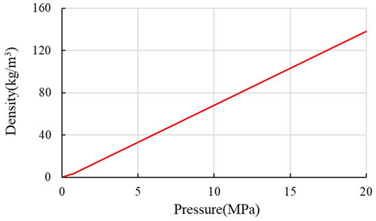
Based on the methane property data from the National Institute of Standards and Technology (NIST) database, the variations in methane density and viscosity with pressure and temperature during the development process are determined, as shown in Figure 1.

Figure 1. Methane–fluid isotherm at 62 °C from NIST database.

A complete description of the gas–water migration process in the shale reservoir requires, in addition to the flow equations mentioned above, a set of auxiliary equations.

The gas–water capillary force equation within the hydraulic fracture system is as follows:

$$p_{Fgw}=p_{Fg}-p_{Fw}$$

(14)

The gas–water saturation equation within the hydraulic fracture system is as follows:

$$s_{\mathrm{F}\mathrm{g}}+s_{\mathrm{F}\mathrm{w}}=1$$

(15)

The gas–water capillary force equation within the shale bedding fracture system is as follows:

$$p_{fgw}=p_{fg}-p_{fw}$$

(16)

The gas–water saturation equation within the shale bedding fracture system is as follows:

$$s_{\mathrm{f}\mathrm{g}}+s_{\mathrm{f}\mathrm{w}}=1$$

(17)

The gas–water capillary force equation in the shale matrix pore system is as follows:

$$p_{mgw}=p_{mg}-p_{wg}$$

(18)

The gas–water saturation equation in the shale matrix pore system is as follows:

$$s_{mg}+s_{m\mathrm{w}}=1$$

(19)

where $p_{Fgw}$ represents the gas–water interfacial tension in hydraulic fractures, MPa; $p_{fgw}$ represents the gas–water interfacial tension in shale bedding fractures, MPa; and $p_{mgw}$ represents the gas–water interfacial tension in matrix pores, MPa.

To achieve a unique solution for the governing equations, a complete set of initial and boundary conditions must be specified.

2.5.1. Inner Boundary Conditions

For a production scenario with a specified bottom-hole flowing pressure, the corresponding gas and water flow rates are calculated using the Peaceman well model, as defined in the following equations:

$$q_{gwell}={\displaystyle \frac{k_{Frg}}{{\mu }_{Fg}{B}_{Fg}\Delta V}}{\displaystyle \frac{2\pi \sqrt{k_{Fx}{k}_{Fy}}\Delta z}{ln\left(\frac{r_e}{r_w}\right)+s}}\left(p_{Fg}-p_{wf}\right)$$

(20)

$$q_{wwell}={\displaystyle \frac{k_{Frw}}{{\mu }_{Fw}{B}_{Fw}\Delta V}}{\displaystyle \frac{2\pi \sqrt{k_{Fx}{k}_{Fy}}\Delta z}{ln\left(\frac{r_e}{r_w}\right)+s}}\left(p_{Fw}-p_{wf}\right)$$

(21)

where

$$r_e=0.28{\displaystyle \frac{{\left[{\left(\frac{k_{Fy}}{k_{Fx}}\right)}^{0.5}{\Delta x}^2+{\left(\frac{k_{Fx}}{k_{Fy}}\right)}^{0.5}{\Delta y}^2\right]}^{0.5}}{{\left(\frac{k_{Fy}}{k_{Fx}}\right)}^{0.25}+{\left(\frac{k_{Fx}}{k_{Fy}}\right)}^{0.25}}}$$

(22)

where $\Delta V$ is the grid volume, m³; $k_{Fx}$ is the hydraulic fracture permeability in x direction, mD; $k_{Fy}$ is the hydraulic fracture permeability in y direction, mD; $\Delta z$ is the reservoir depth, m; $r_e$ is the drainage radius, m; $r_w$ is the wellbore radius, m; $s$ is the skin factor, dimensionless; $p_{wf}$ is the downhole flowing pressure, MPa; $\Delta x$ is the grid size in x direction, m; and $\Delta y$ is the grid size in y direction, m.

2.5.2. Outer Boundary Conditions

The outer boundary is a closed boundary and belongs to the second type of boundary condition.

$$\begin{gathered} {\left.p_{fg}\left(x,y,z,t\right)\right|}_{\mathsf{\Gamma }}=p_{fg1}\left(x,y,z,t\right) \\ {\left.p_{fw}\left(x,y,z,t\right)\right|}_{\mathsf{\Gamma }}=p_{fw1}\left(x,y,z,t\right) \\ {\left.p_{mg}\left(x,y,z,t\right)\right|}_{\mathsf{\Gamma }}=p_{mg1}\left(x,y,z,t\right) \\ {\left.p_{mw}\left(x,y,z,t\right)\right|}_{\mathsf{\Gamma }}=p_{mw1}\left(x,y,z,t\right) \end{gathered}$$

(23)

where $\Gamma$ is the outer boundary, m; $p_{fg1}\left(x,y,z,t\right)$ is the known gas pressure for the bedding fracture boundary, MPa; $p_{fw1}\left(x,y,z,t\right)$ is the known water pressure for the bedding fracture boundary, MPa; $p_{mg1}\left(x,y,z,t\right)$ is the known gas pressure for the matrix pore boundary, MPa; and $p_{mw1}\left(x,y,z,t\right)$ is the known water pressure for the matrix pore boundary, MPa.

2.5.3. Initial Conditions

The initial conditions for the simulation are defined by the distribution of reservoir pressure, water saturation, and gas content at the start of production.

$$\begin{gathered} {\left.p_{Fg}\left(x,y,z\right)\right|}_{t=0}=p_{Fg0}\left(x,y,z\right),{\left.p_{fg}\left(x,y,z\right)\right|}_{t=0}=p_{fg0}\left(x,y,z\right), \\ {\left.p_{mg}\left(x,y,z\right)\right|}_{t=0}=p_{mg0}\left(x,y,z\right),{\left.p_{Fw}\left(x,y,z\right)\right|}_{t=0}=p_{Fw0}\left(x,y,z\right), \\ {\left.p_{fw}\left(x,y,z\right)\right|}_{t=0}=p_{fw0}\left(x,y,z\right),{\left.p_{mw}\left(x,y,z\right)\right|}_{t=0}=p_{mw0}\left(x,y,z\right), \\ {\left.s_{Fg}\left(x,y,z\right)\right|}_{t=0}=s_{Fg0}\left(x,y,z\right),{\left.s_{fg}\left(x,y,z\right)\right|}_{t=0}=s_{fg0}\left(x,y,z\right), \\ {\left.s_{mg}\left(x,y,z\right)\right|}_{t=0}=s_{mg0}\left(x,y,z\right),{\left.s_{Fw}\left(x,y,z\right)\right|}_{t=0}=s_{Fw0}\left(x,y,z\right), \\ {\left.s_{fw}\left(x,y,z\right)\right|}_{t=0}=s_{fw0}\left(x,y,z\right),{\left.s_{mw}\left(x,y,z\right)\right|}_{t=0}=s_{mw0}\left(x,y,z\right), \\ {\left.V_m\left(x,y,z\right)\right|}_{t=0}=V_{m0}\left(x,y,z\right) \end{gathered}$$

(24)

where $p_{Fg0}\left(x,y,z\right)$ is the initial gas pressure for hydraulic fractures, MPa; $p_{fg0}\left(x,y,z\right)$ is the initial gas pressure for bedding fractures, MPa; $p_{mg0}\left(x,y,z\right)$ is the initial gas pressure for matrix pores, MPa; $p_{Fw0}\left(x,y,z\right)$ is the initial water pressure for hydraulic fractures, MPa; $p_{fw0}\left(x,y,z\right)$ is the initial water pressure for bedding fractures, MPa; $p_{mw0}\left(x,y,z\right)$ is the initial water pressure for matrix pores, MPa; $s_{Fg0}\left(x,y,z\right)$ is the initial gas saturation for hydraulic fractures, dimensionless; $s_{fg0}\left(x,y,z\right)$ is the initial gas saturation for bedding fractures, dimensionless; $s_{mg0}\left(x,y,z\right)$ is the initial gas saturation for matrix pores, dimensionless; $s_{Fw0}\left(x,y,z\right)$ is the initial water saturation for hydraulic fractures, dimensionless; $s_{fw0}\left(x,y,z\right)$ is the initial water saturation for bedding fractures, dimensionless; $s_{mw0}\left(x,y,z\right)$ is the initial water saturation for matrix pores, dimensionless; and $V_{m0}\left(x,y,z\right)$ is the initial gas adsorption within matrix pores, dimensionless.

2.6. Model Solution

The numerical solution for the two-phase (gas and water) flow-governing equations in the shale gas reservoir is obtained using a fully implicit method. This approach is adopted to handle the strong nonlinearity arising from the coupling of flow and geomechanical responses, which is particularly pronounced under stress-sensitive conditions. The discrete nonlinear system is linearized via Newton’s method and solved iteratively, generating a large-scale, asymmetric, block-banded sparse linear system at each iteration. Preconditioned iterative solvers are employed to solve these linear equations efficiently. Through the arrangement and elimination of variables, the final system to be solved is expressed in terms of the primary variable increments. These increments, denoted as $\delta p_{Fg}$, $\delta p_{Fw}$, $\delta p_{fg}$, $\delta p_{fw}$, $\delta p_{mg}$, $\delta p_{mw}$, $\delta s_{Fg}$, $\delta s_{Fw}$, $\delta s_{fg}$, $\delta s_{fw}$, $\delta s_{mg}$, and ${\delta s}_{mw}$, form a linear system that can be expressed in matrix form as follows:

$$AX=b$$

(25)

where A is the coefficient matrix of the equation system.

To solve this linear system, we employ the Generalized Minimal Residual (GMRES) method, preconditioned with a block-based incomplete LU (ILU) decomposition.

3. Results and Analysis

3.1. History Matching

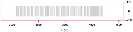
A geometric model for the hydraulically fractured horizontal well X1H was developed based on an integrated dataset comprising its wellbore configuration, reservoir properties, and fracturing treatment parameters, as illustrated in Figure 2. The corresponding parameters and their sources were also summarized in Table 1.

Figure 2. Geometric model diagram for shale gas fractured horizontal well X1H.

Table 1. Parameters of the well X1H.

Parameters	Units	Values	Sources
Reservoir Length	m	2300	Oilfield Development Plan
Reservoir Width	m	350	Oilfield Development Plan
Reservoir Depth	m	4	Oilfield Development Plan
Buried Depth	m	2300	Drilling Design Report
Pressure Coefficient	-	0.87	Well Logging Report
Reservoir Temperature	°C	62	Well Logging Report
Matrix Porosity	%	3	Core Analysis and History Matching
Matrix Permeability	mD	0.0001	Core Analysis and History Matching
Initial Bedding Fracture Porosity	%	0.5	Core Analysis and History Matching
Initial Bedding Fracture Permeability	mD	0.00435	Core Analysis and History Matching
Stress Sensitivity Coefficient for Bedding Fracture	MPa−1	0.76	Core Analysis and History Matching
Hydraulic Fracture Half Length	m	100	Fracturing Report
Hydraulic Fracture Width	m	0.02	Fracturing Report
Hydraulic Fracture Height	m	10	Fracturing Report
Hydraulic Fracture Conductivity	D × cm	0.5	Fracturing Report
Gas Content in the Matrix Pore	m3/t	3.8	Well Logging Report
Gas Saturation in the Bedding Fracture	%	52.9	Well Logging Report
Langmuir Pressure	MPa	1.26	Core Analysis and History Matching
Langmuir Volume	m3/t	2.06	Core Analysis and History Matching
Critical Desorption Pressure	MPa	10	Drainage Report

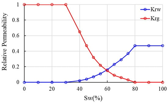
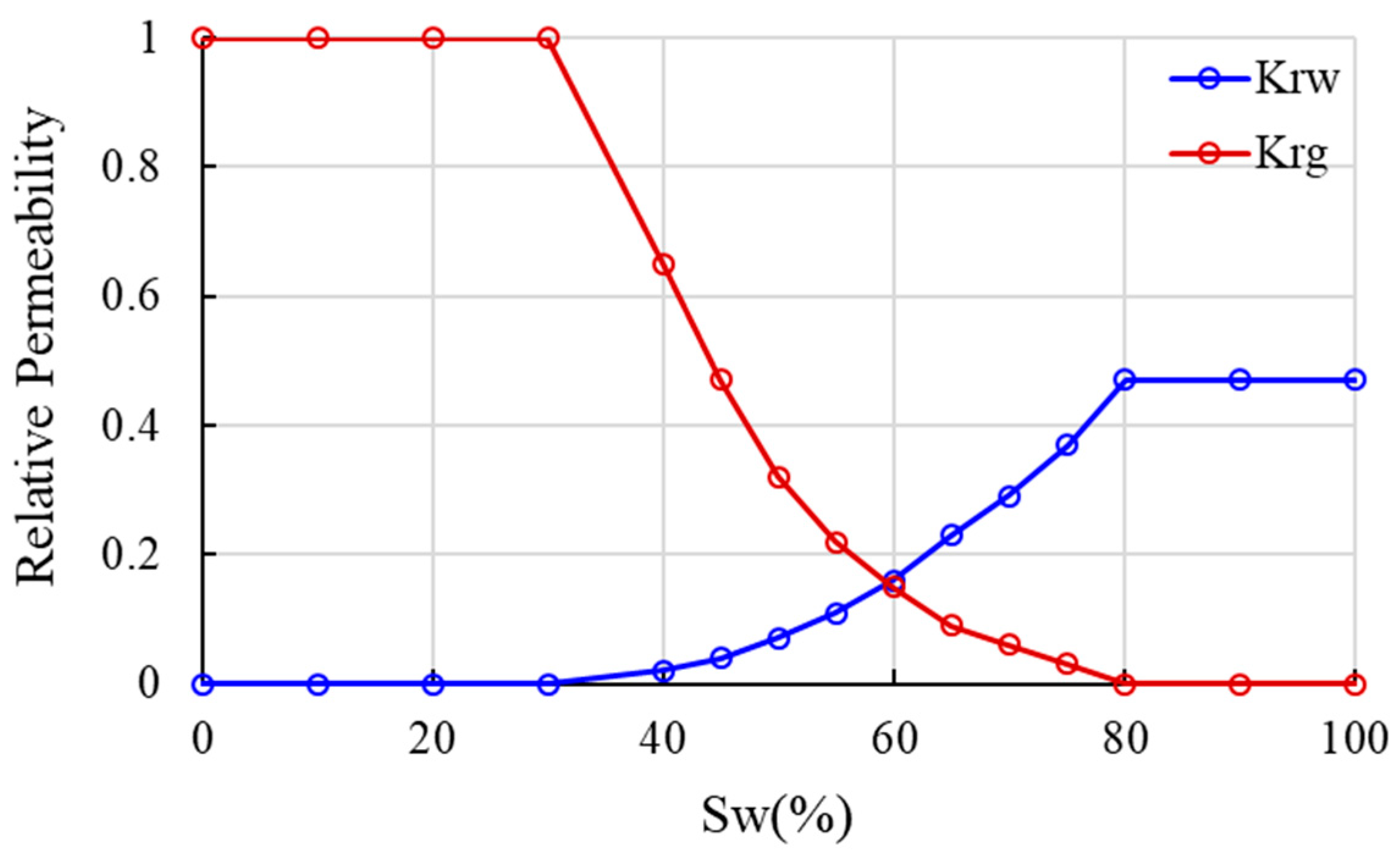
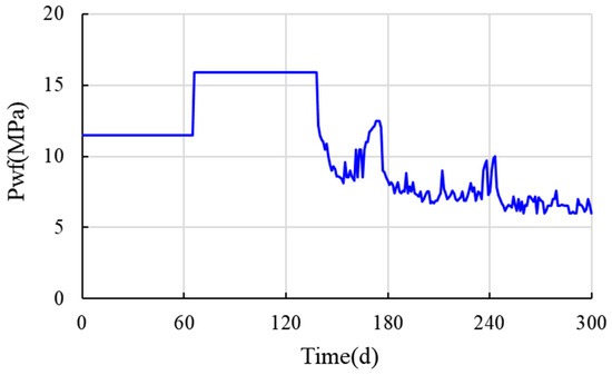
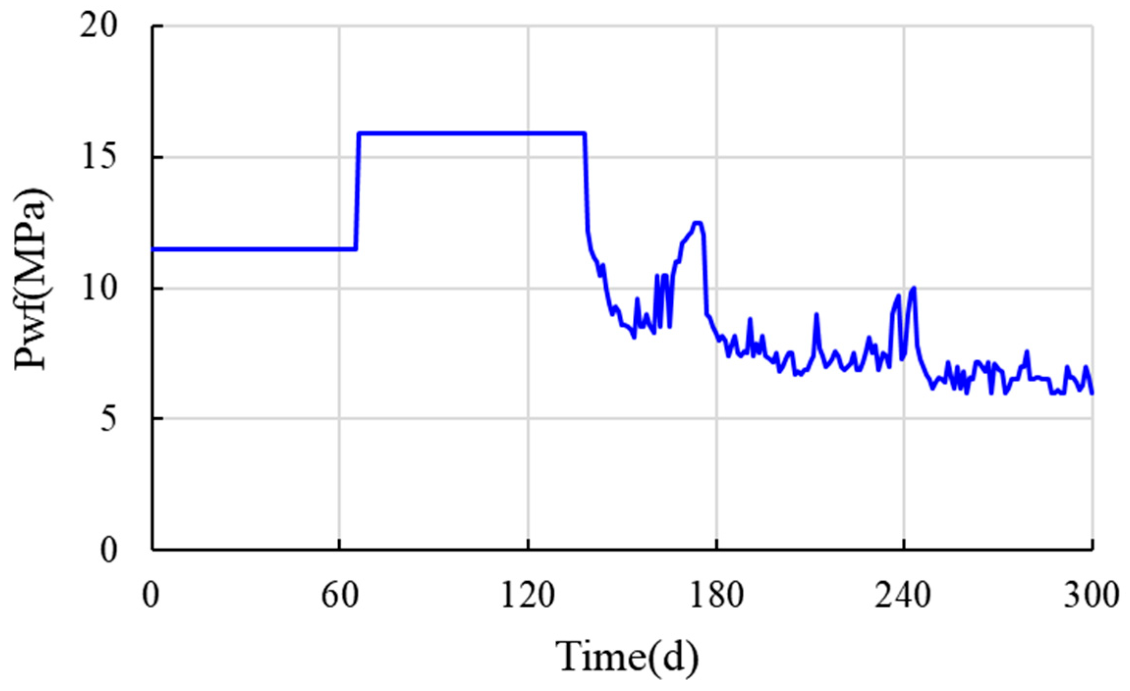
The phase permeability under formation conditions was determined using simulated gas–water relative permeability data (Figure 3). Furthermore, the recorded daily production history of well X1H was used to constrain the simulated bottom-hole flowing pressure, as shown in Figure 4.

Figure 3. Gas–water relative permeability for well X1H.

Figure 4. Recorded daily bottom-hole flowing pressure of well X1H.

The production drainage simulation and history matching of well X1H were conducted over a 300-day period. The history matching process determined key characteristic parameters, including matrix porosity, matrix permeability, initial bedding fracture porosity, initial bedding fracture permeability, stress sensitivity coefficient for bedding fracture, Langmuir pressure, and Langmuir volume (Table 1).

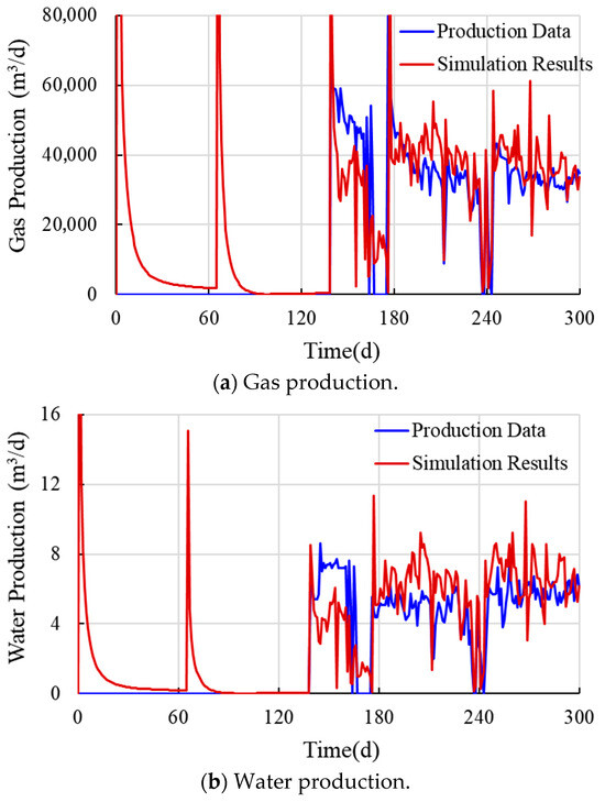
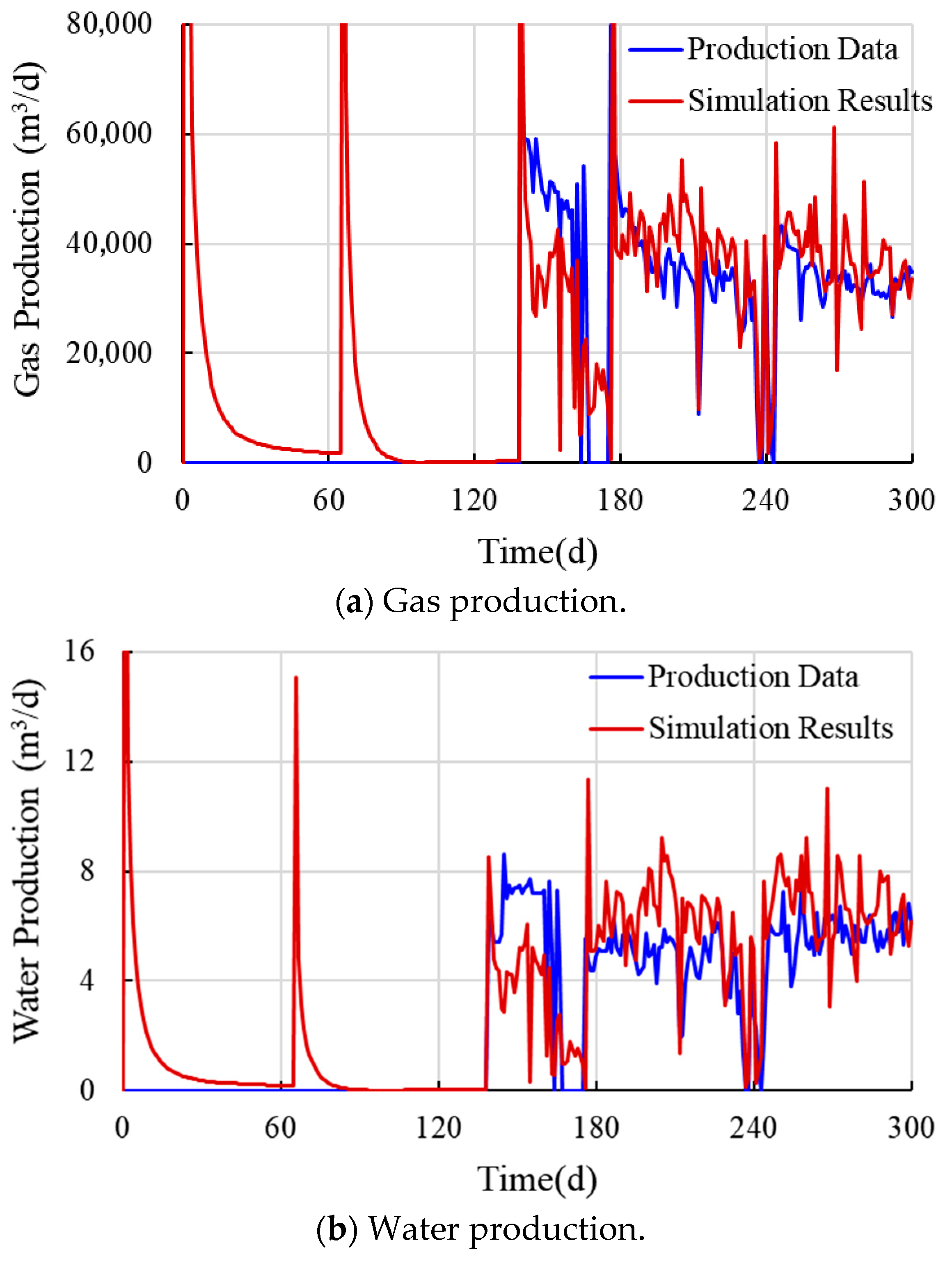
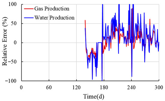
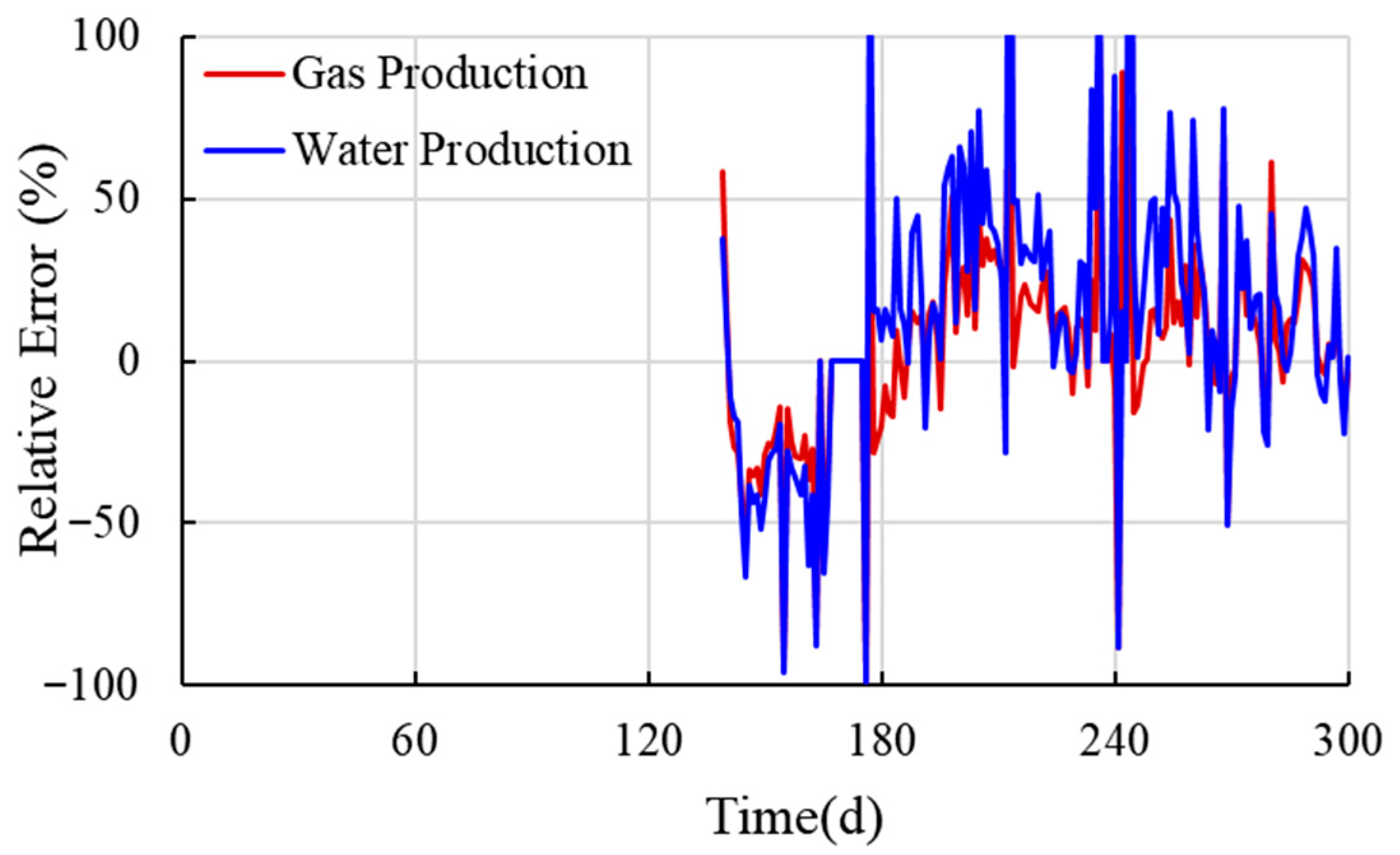
The flow regimes evolved through distinct stages. Early production was characterized by linear or bilinear behavior within the fracture network, where productivity was governed by fracture volume and conductivity. This initial stage transitioned into a prolonged formation linear flow period, dominated by fluid migration from the matrix into the fractures. Consequently, the history matching assigned different parameter groups to different production stages: parameters related to hydraulic fractures were primarily fitted against flowback data, bedding fracture parameters against initial production data, and matrix parameters against stable production data. While multiple factors influence permeability, stress sensitivity is identified as a primary cause of its significant variation. Furthermore, gas desorption from the shale matrix further contributes to the sustained production during the latter stage. The history matching results for both gas production and water drainage are shown in Figure 5. The mean relative errors for gas and water production were 21.94% and 33.18%, respectively, as shown in Figure 6. The average relative error for the gas phase is greater than that for the liquid phase. This discrepancy arises because the history matching was calibrated primarily against the dynamic bottom-hole flowing pressure, with gas production as the key matching parameter and liquid production as a secondary reference. A notably high average relative error of 34.48% for gas production occurs between days 139 and 166. This is due to the absence of gas production in the first 139 days, which led to gas accumulation in the wellbore. The subsequent release of this accumulated gas resulted in a production surge that the model did not fully replicate, hence the larger error during this period.

Figure 5. Comparison between production data and simulation results for well X1H.

Figure 6. Deviations between the production data and simulation results for well X1H.

3.2. Sensitivity Analysis

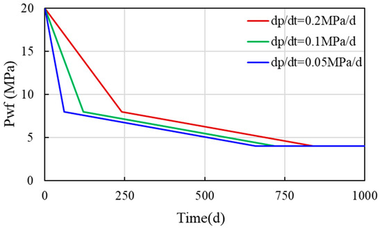
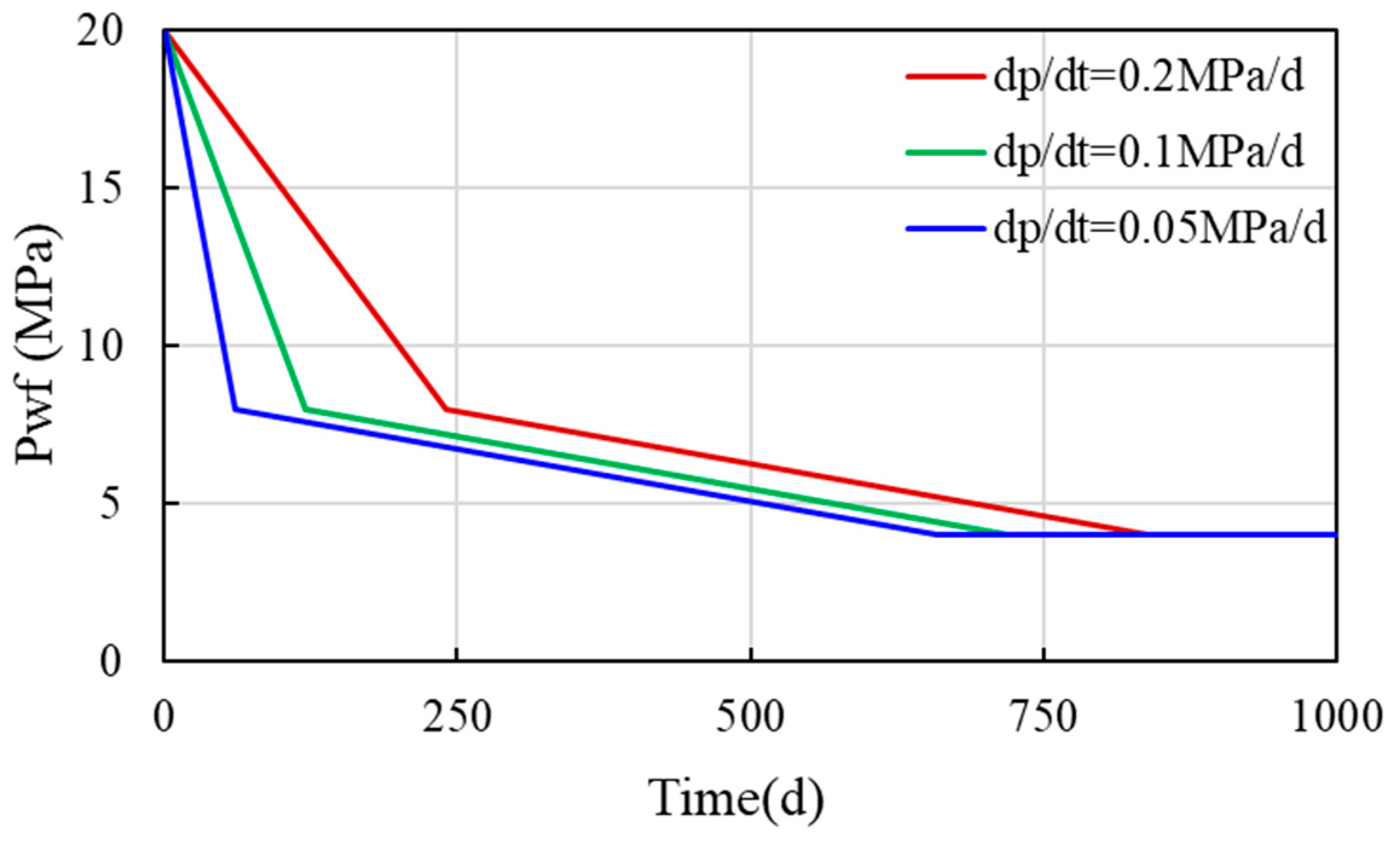
Based on the drainage data of well X1H, the pressure depletion strategies with different decline rates are discussed. All the strategies involved an initial rapid depletion from 20 MPa to 8 MPa, followed by a smooth depletion to 4 MPa. The variable parameter was the initial pressure depletion rate, which was set at 0.05 MPa/d, 0.1 MPa/d, and 0.2 MPa/d, as shown in Figure 7.

Figure 7. Bottom-hole flowing pressure depletion strategies with different initial decline rates.

3.2.1. Initial Permeability for Bedding Fractures

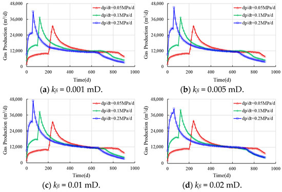
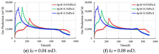
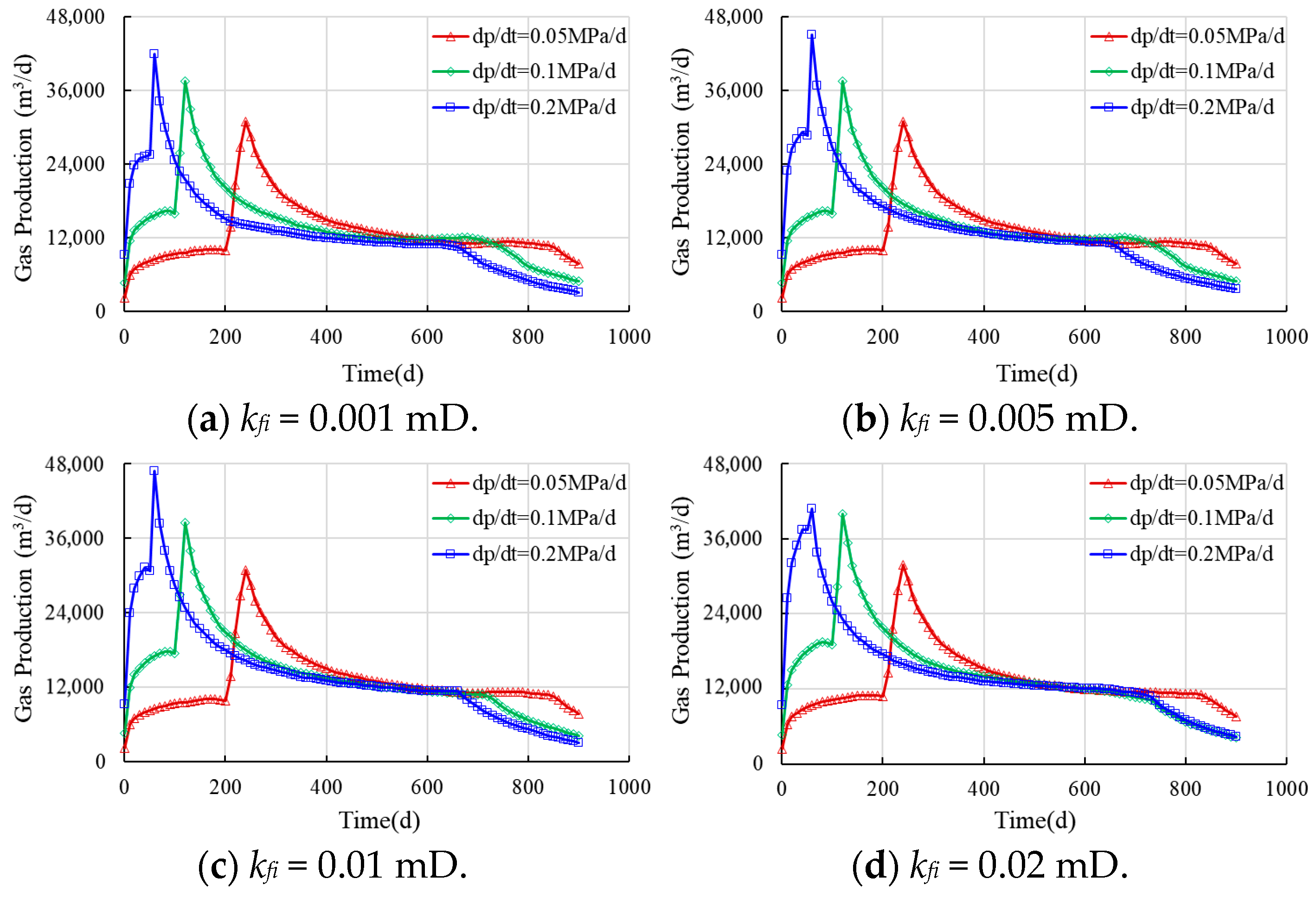
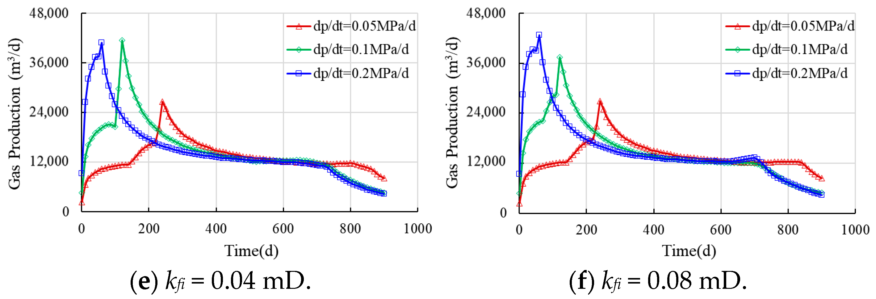
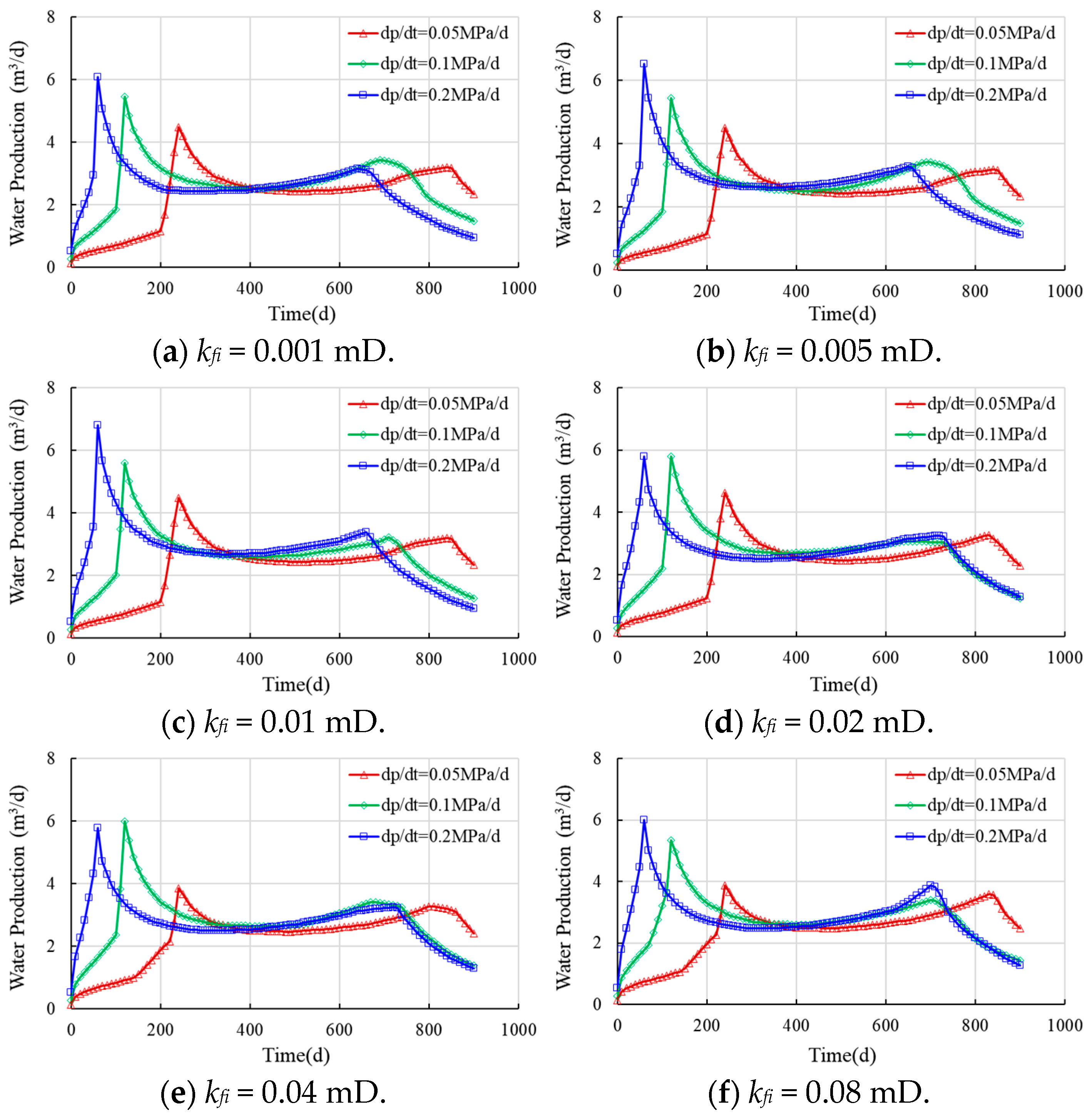
The effect of initial bedding fracture permeability on horizontal well performance was simulated, and the results are summarized in Figure 8 and Figure 9. The water production rate initially increases rapidly to a peak and then decreases slightly and stabilizes. When the bottom-hole flowing pressure stabilizes, the water rate declines further. The peak water rates for the three initial liquid drainage rates occur at 60, 120, and 240 days, respectively, which is consistent with the defined pressure decline strategies.

Figure 8. Effects of initial bedding fracture permeability on gas production.

Figure 9. Effects of initial bedding fracture permeability on water production.

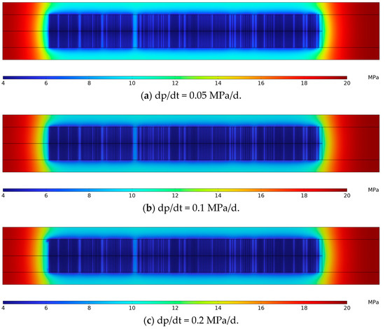
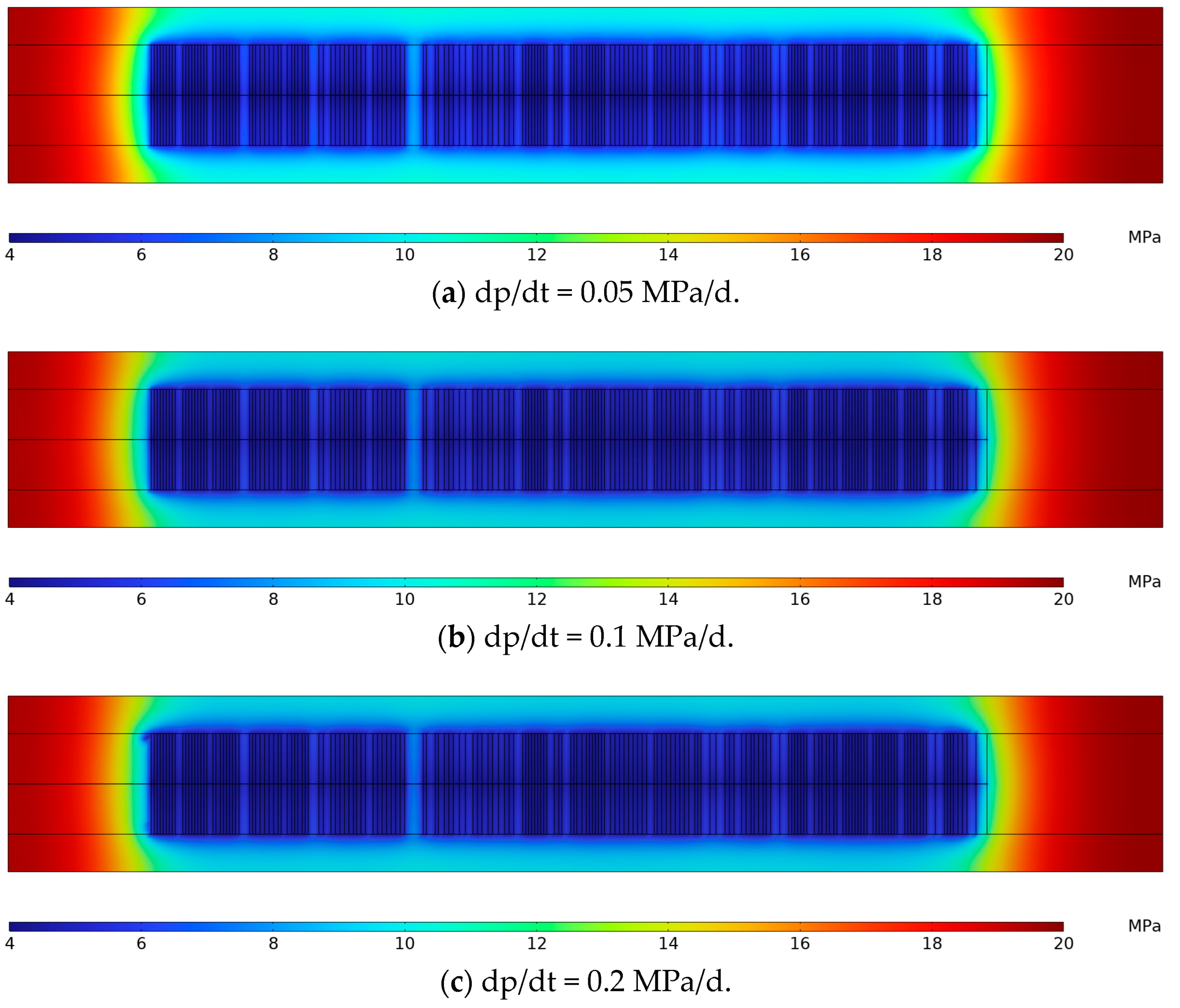
Figure 8 and Figure 9 also indicate that both gas production and water drainage are not significantly affected by initial permeability but are notably influenced by pressure decline rate. Compared to the base case with 0.005 mD, the cumulative gas production rate changes by −2.29% (0.001 mD), +0.80% (0.01 mD), +3.30% (0.02 mD), +4.51% (0.04 mD), and +6.21% (0.08 mD). While a rapid pressure decline rate of 0.2 MPa/d achieves a 30–50% increase in peak production compared to a gradual depletion case of 0.05 MPa/d, the cumulative production differences are typically within 10%. The drainage radius derived from pressure contours further shows that rapid depletion (0.2 MPa/d) increases production by an average of 15% compared to gradual depletion (0.05 MPa/d), as illustrated in Figure 10. Notably, for permeabilities above 0.04 mD, production shows a more pronounced increase before peaking, suggesting a threshold below which flow is constrained by bedding-plane fractures. Above this threshold, the dominant flow limitation, or “blockage point”, shifts to the bedding fracture system. This finding suggests that while gas can readily desorb from the matrix pore and flow through the bedding fracture, it encounters greater resistance within the hydraulic fracture. The well’s productivity is constrained by the flow conductivity of the hydraulic fracture network. Overall, rapid initial drainage is beneficial for expanding the drainage radius. Based on these results, we recommend an initial depletion rate of 0.1 MPa/d for reservoirs with an initial permeability ranging from 0.001 to 0.005 mD and a higher rate of 0.2 MPa/d for an initial permeability greater than 0.005 mD.

Figure 10. Pressure contours for different initial pressure depletion strategies.

3.2.2. Stress Sensitivity for Bedding Fractures

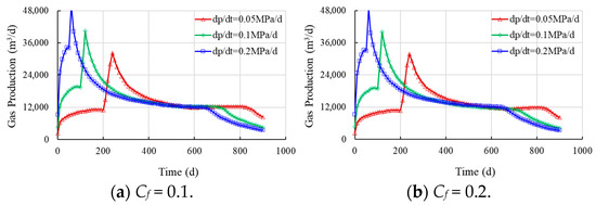
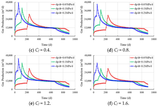
Similarly, the impact of bedding fracture stress sensitivity on horizontal well performance was simulated, with the results presented in Figure 11 and Figure 12. According to previous studies, the stress sensitivity coefficients for transitional shale gas reservoirs range from 0.1 to 1.6 [19,20,21].

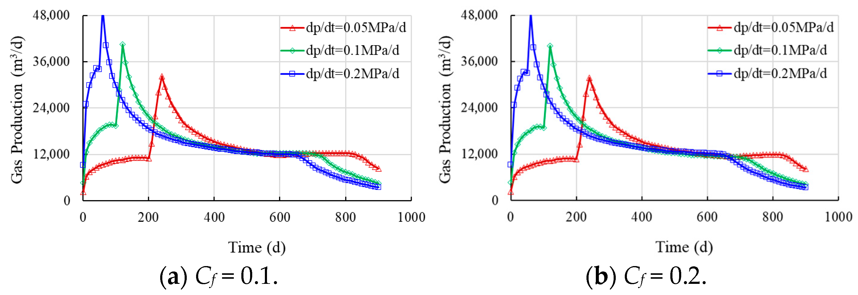
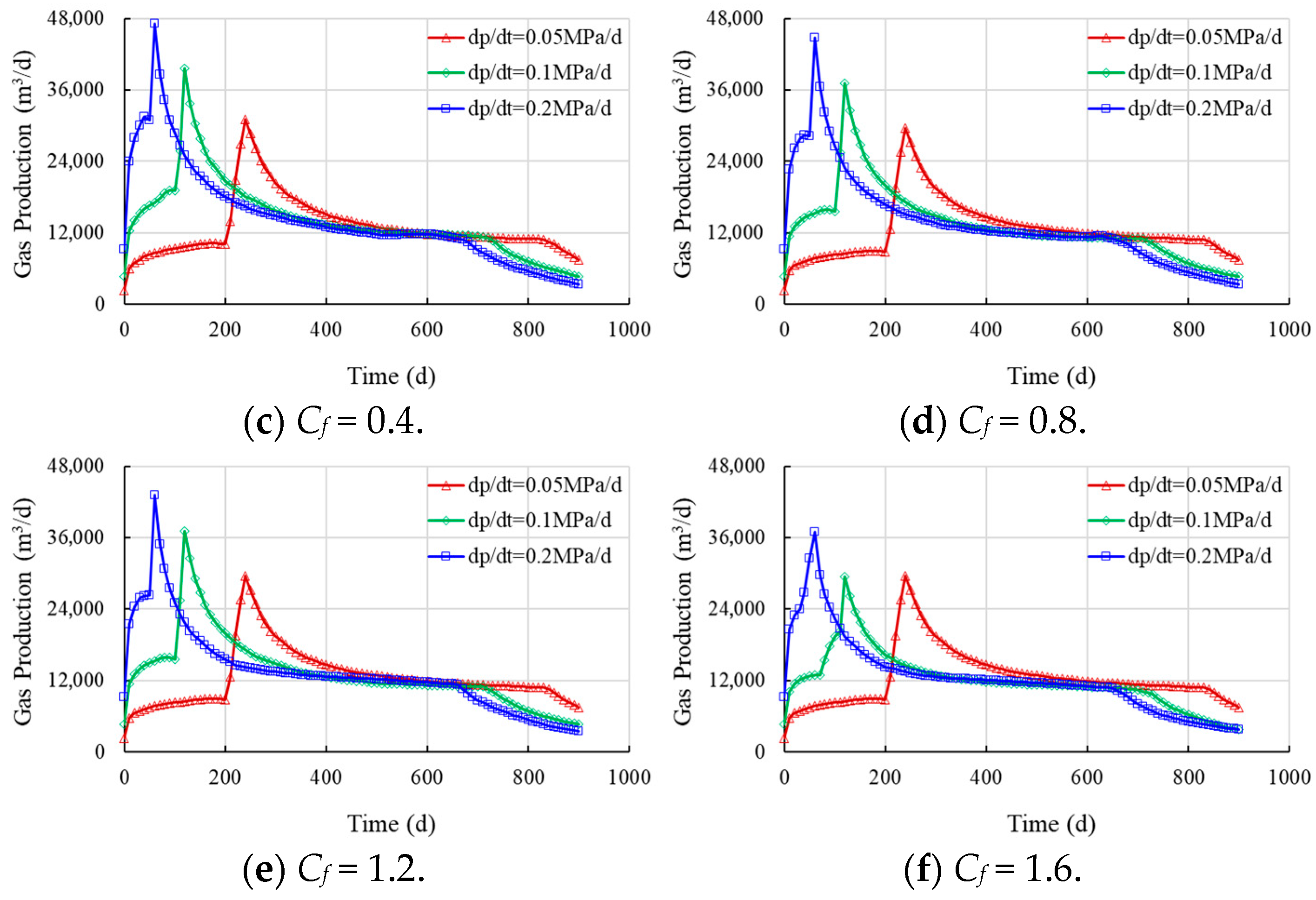
Figure 11. Effects of stress sensitivity coefficient on gas production.

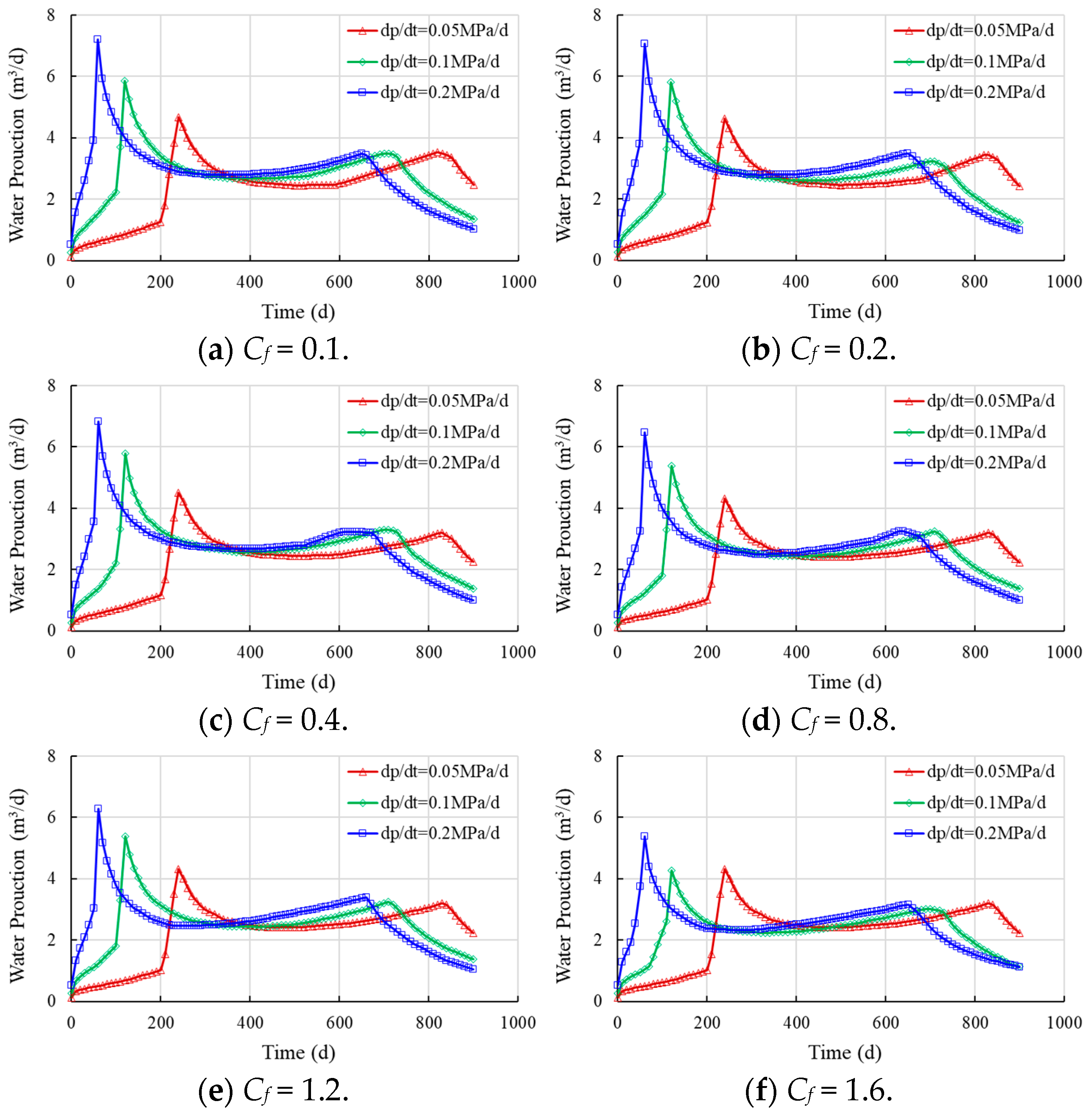
Figure 12. Effects of stress sensitivity coefficient on water production.

Figure 11 and Figure 12 indicate that the shale gas production rate initially increases rapidly to a peak and then undergoes a gradual decline and stabilization. A further decrease occurs once the bottom-hole flowing pressure stabilizes. During the initial drainage stage, production consists primarily of free gas, manifested as a rapid rise in the gas production rate. The pressure depletion funnel expands radially during this period, and the extent of this expansion is a key determinant of ultimate recovery. After the bottom-hole flowing pressure falls below the critical desorption pressure, significant gas desorption occurs within the depleted region, leading to a further increase in gas production. This phase involves a complex interaction between pressure-driven and desorption-driven supply. If the flowing pressure decline is too gradual, the desorbed gas may accumulate in the bedding fractures instead of being produced, thereby reducing the peak gas production rate. Conversely, if the flowing pressure decline is too rapid, the volume of desorbed gas may be insufficient to replenish the fractures, leading to a steep production decline.

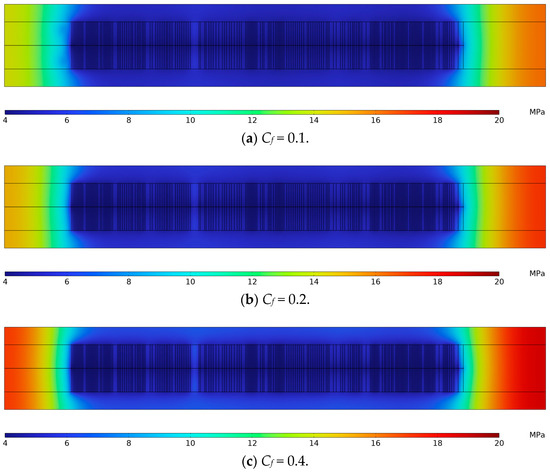
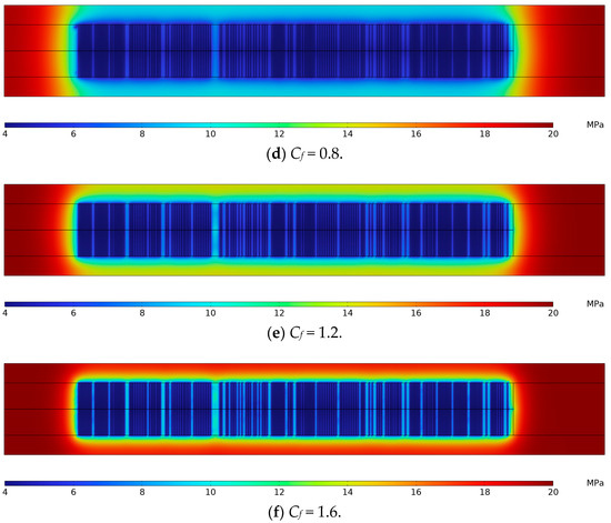
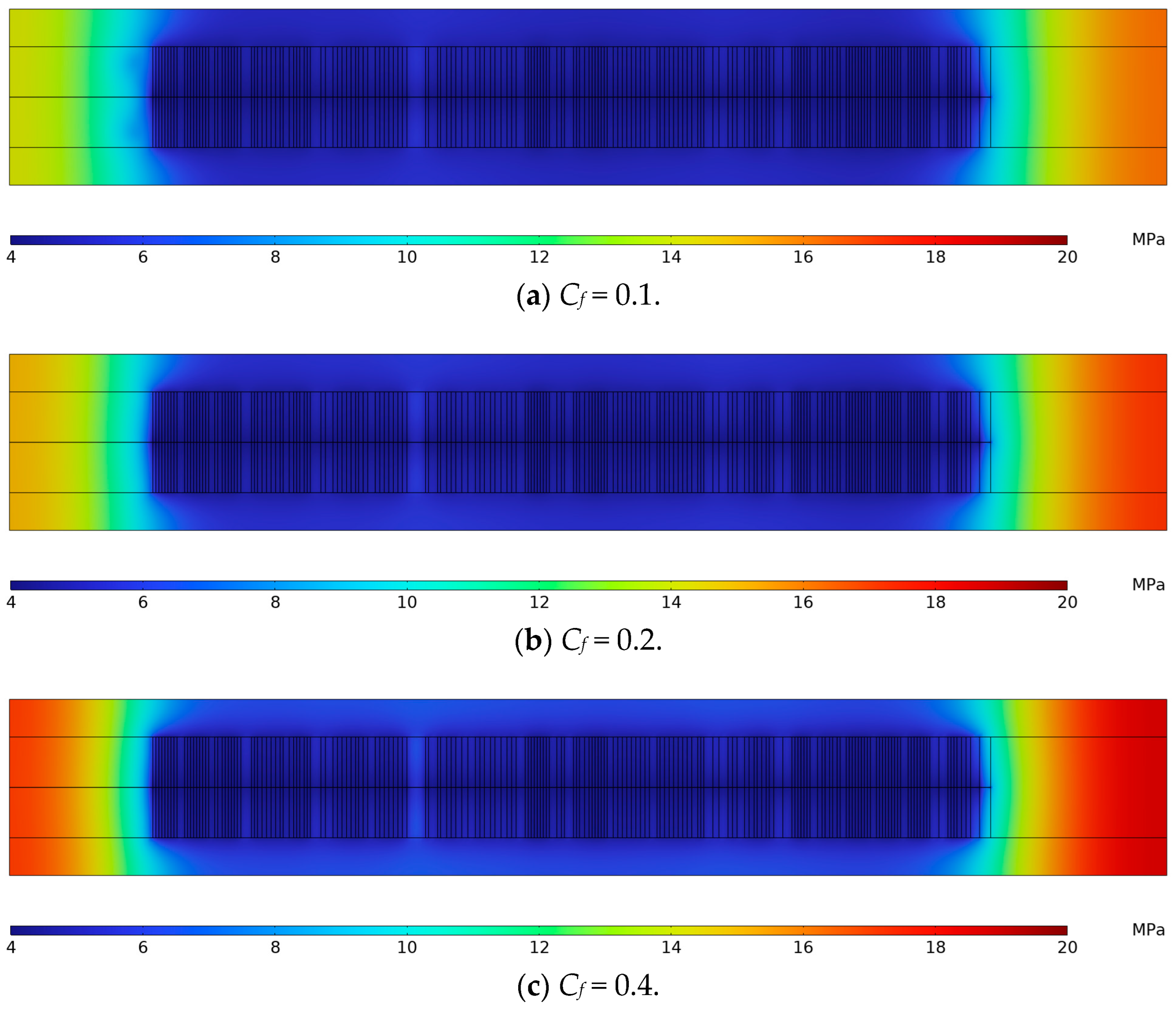
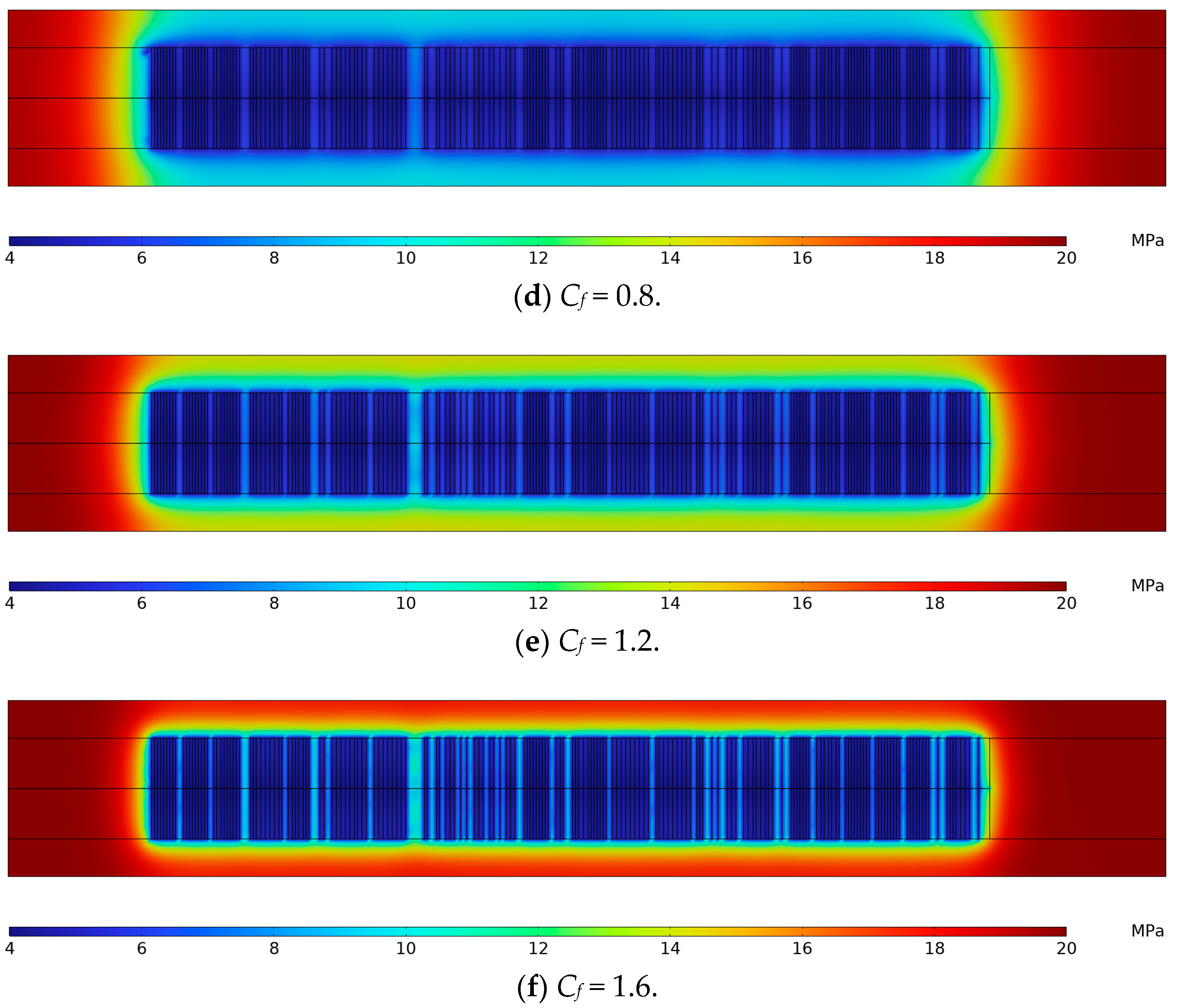
The results demonstrate a strong dependence of well performance on both the stress sensitivity coefficient and pressure decline rate. Compared to the base case (C_f = 0.8), the gas production rate changes by +9.38% (C_f = 0.1), +7.20% (C_f = 0.2), +4.73% (C_f = 0.4), −0.80% (C_f = 1.2), and −5.58% (C_f = 1.6). While a rapid pressure decline rate of 0.2 MPa/d achieves a 20–65% higher peak production than a gradual depletion of 0.05 MPa/d, the cumulative production difference remains within 11%. As the stress sensitivity coefficient increases, the resulting permeability reduction hinders the expansion of the drainage radius, causing an average decline of over 20% in peak gas and water production, as shown in Figure 13. The significant contrast in pressure contours further suggests that for stress sensitivity coefficients larger than 0.8, the primary flow obstruction shifts towards the matrix pores. Based on these findings, an initial pressure depletion rate of 0.2 MPa/d is recommended; for reservoirs with a stress sensitive coefficient below 0.8, it is recommended that the initial liquid drainage rate be set at 0.2 MPa/d. For coefficients of 1.2 and higher, a more conservative rate of 0.1 MPa/d is advised to minimize the negative impact on productivity.

Figure 13. Pressure contours for different stress sensitivity coefficients.

4. Conclusions

In this study, a multiscale modeling approach was employed to investigate the effects of stress sensitivity and pressure decline rate on the productivity of horizontal wells in transitional shale gas reservoirs. The simulation results yield the following conclusions and operational recommendations.

(1) The rapid fluid drainage during the initial production stage helps to expand the drainage radius. Specifically, a depletion rate of 0.2 MPa/d increases gas production by approximately 10% compared to a rate of 0.05 MPa/d.

(2) Stress sensitivity reduces gas production by up to 20%. In adjacent wells with a stress sensitivity coefficient greater than 0.8, the blocking zones may extend into the matrix pores. Therefore, operational strategies should aim to mitigate stress sensitivity effects.

(3) Well-connected bedding fracture can improve gas production by about 5%. For well X1H, gas and water appear to be blocked within the fracture network under conditions. Thus, implementing measures to enhance flow conductivity is recommended.

References

- Mehmet, M. Shale gas: Analysis of its role in the global energy market. Renew. Sustain. Energy Rev. 2014, 37, 460–468. [Google Scholar] [CrossRef] [Scilit]
- Wang, J.Y.; Guo, S.B. Comparison of geochemical characteristics of marine facies, marine-continental transitional facies and continental facies shale in typical areas of China and their control over organic-rich shale. Energy Sources Part A Recovery Util. Environ. Eff. 2024, 46, 12512–12524. [Google Scholar] [CrossRef] [Scilit]
- Guo, X.S.; Wang, R.Y.; Shen, B.J.; Wang, G.P.; Wan, C.X.; Wang, Q.R. Geological characteristics, resource potential, and development direction of shale gas in China. Pet. Explor. Dev. 2025, 52, 17–32. [Google Scholar] [CrossRef] [Scilit]
- Wu, J.; Tan, J.Q.; Xu, J.Q.; Elsworth, D. Challenges to sustainable large-scale shale gas development in China. Proc. Natl. Acad. Sci. USA 2025, 122, e2415192122. [Google Scholar] [CrossRef] [Scilit]
- Ma, X.H.; Xie, J. The progress and prospects of shale gas exploration and development in southern Sichuan Basin, SW China. Pet. Explor. Dev. 2018, 45, 443–451. [Google Scholar] [CrossRef] [Scilit]
- Li, Y.; Zhou, D.H.; Wang, W.H.; Jiang, T.X.; Xue, Z.J. Development of unconventional gas and technologies adopted in China. Energy Geosci. 2020, 1, 55–68. [Google Scholar] [CrossRef] [Scilit]
- Li, Q.Q.; Xu, S. Research status and prospects of marine-continental transitional shale reservoirs. Geol. Bull. China 2022, 41, 1417–1429. [Google Scholar] [CrossRef]
- Xu, K.; Chen, S.J.; Tao, Z.Q.; Lu, J.G.; He, Q.B.; Li, C. Controlling factors and quantitative characterization of pore development in marine-continental transitional shale. Lithosphere 2022, 2022, 6290684. [Google Scholar] [CrossRef] [Scilit]
- Liang, Q.S.; Zhang, X.; Tian, J.C.; Sun, X.; Chang, H. Geological and geochemical characteristics of marine-continental transitional shale from the Lower Permian Taiyuan Formation, Taikang Uplift, southern North China Basin. Mar. Pet. Geol. 2018, 98, 229–242. [Google Scholar] [CrossRef] [Scilit]
- Zhang, J.Z.; Li, X.Q.; Zhang, X.Q.; Zhang, M.; Cong, G.S.; Zhang, G.W.; Wang, F.Y. Geochemical and geological characterization of marine–continental transitional shales from Longtan formation in Yangtze area, South China. Mar. Pet. Geol. 2018, 96, 1–15. [Google Scholar] [CrossRef] [Scilit]
- Jiao, P.F.; Yao, G.S.; Zhou, S.W.; Yu, Z.; Wang, S.L. A comparative study of the micropore structure between the transitional and marine shales in China. Geofluids 2021, 2021, 5562532. [Google Scholar] [CrossRef] [Scilit]
- Cao, T.T.; Deng, M.; Xiao, J.Y.; Liu, H.; Pan, A.Y.; Cao, Q.G. Reservoir characteristics of marine–continental transitional shale and gas-bearing mechanism: Understanding based on comparison with marine shale reservoir. J. Nat. Gas Geosci. 2023, 8, 169–185. [Google Scholar] [CrossRef] [Scilit]
- Liu, L.L.; Li, J.; Zhou, S.X.; Chen, G.R.; Li, Y.Y.; Pang, W.J.; Wang, H. Comparative study on flow characteristics in deep marine and marine–continental transitional shale in the Southeastern Sichuan Basin, China. ACS Omega 2024, 9, 22016–22030. [Google Scholar] [CrossRef] [Scilit]
- Li, Y.; Zhang, Q.; Li, S.X.; Guo, B.Z.; He, Q.B.; Lu, J.G.; Zhao, L.P.; Ma, Z.W. Methane adsorption characteristics of marine-continental transitional shales based on the experimental study of Shanxi formation of the Lower Permian in the Ordos basin. Energy Fuels 2024, 38, 21984–21999. [Google Scholar] [CrossRef] [Scilit]
- Chen, M.J.; Ning, X.Y.; Kang, Y.L.; Wu, J.G.; Li, B.; Shi, Y.; Lai, Z.H.; Bai, J.J.; Yan, M.L. Effect of fracturing fluid properties on the flowback efficiency of marine and continental transitional shale gas reservoirs in Ordos basin. Processes 2025, 13, 1398. [Google Scholar] [CrossRef] [Scilit]
- Han, S.B.; Huang, J.; Xiang, C.H.; Xie, L.F.; Tang, Z.Y.; Chen, C.; Zhang, J.C. Pore structure and fractal characteristics of marine-continental transitional shales in the southern North China Basin. Interpretation 2022, 10, B25-T911. [Google Scholar] [CrossRef] [Scilit]
- Peng, H.J.; Zhao, J.Z.; Qiu, Z.; Zhang, Q.; Liu, W.; Kong, W.L.; Gao, W.L.; Sheng, T.J.; Li, W.Y.; Yang, Y.G. Multi-scale fracture characterization method for transitional shale reservoir based on post-stack multi-attribute ant-tracking fusion and pre-stack wide-azimuth gathers AVAZ analysis. Geomech. Geophys. Geo-Energy Geo-Resour. 2025, 11, 13. [Google Scholar] [CrossRef] [Scilit]
- Wang, W.L.; Dong, L.; Tan, C.Q.; Yin, S.; Li, A.R.; Wang, R.Y. Developmental characteristics and dominant factors of fractures in marine–continental transitional facies tight sandstone reservoirs in heavily deformed areas: A case study. Arab. J. Geosci. 2020, 13, 473. [Google Scholar] [CrossRef] [Scilit]
- Zhang, W.T.; Wang, Q.; Ning, Z.F.; Zhang, R.; Huang, L.; Cheng, Z.L. Relationship between the stress sensitivity and pore structure of shale. J. Nat. Gas Sci. Eng. 2018, 59, 440–451. [Google Scholar] [CrossRef] [Scilit]
- Wu, Z.H.; Zuo, Y.J.; Wang, S.Y.; Sunwen, J.B.; Liu, L.L. Experimental study on the stress sensitivity and influence factors of shale under varying stress. Shock Vib. 2018, 2018, 3616942. [Google Scholar] [CrossRef] [Scilit]
- Su, Y.L.; Wang, C.W.; Li, L.; Wang, W.D.; Hao, Y.M.; Rezaei-Gomari, S. Experimental on physical properties of shale gas under low-velocity seepage and stress sensitivity environment. J. Pet. Sci. Eng. 2022, 218, 110974. [Google Scholar] [CrossRef] [Scilit]
- Grabowska, J.; Blazquez, S.; Sanz, E.; Zeron, I.M.; Algaba, J.; Miguez, J.M.; Blas, F.J.; Vega, C. Solubility of methane in water: Some useful results for hydrate nucleation. J. Phys. Chem. B 2022, 126, 8553–8570. [Google Scholar] [CrossRef] [Scilit]
- Zeng, Q.S.; Wang, Z.M. A new cleat volume compressibility determination method and the corresponding modification to coal permeability model. Transp. Porous Media 2017, 119, 689–706. [Google Scholar] [CrossRef] [Scilit]
- Mukherjee, M.; Vishal, V. Gas transport in shale: A critical review of experimental studies on shale permeability at a mesoscopic scale. Earth-Sci. Rev. 2023, 244, 104522. [Google Scholar] [CrossRef] [Scilit]
- Pang, Y.; Soilman, M.Y.; Deng, H.; Emadi, H. Analysis of effective porosity effective permeability in shale-gas reservoirs with consideration of gas adsorption stress effect. SPE J. 2017, 22, 1739–1759. [Google Scholar] [CrossRef] [Scilit]
- Xu, Y.; Cavalcante Filho, J.S.A.; Yu, W.; Sepehrnoori, K. Discrete-fracture modeling of complex hydraulic-fracture geometries in reservoir simulators. SPE Reserv. Eval. Eng. 2017, 20, 403–422. [Google Scholar] [CrossRef] [Scilit]
- Xu, Y.; Sepehrnoori, K. Development of an embedded discrete fracture model for field-scale reservoir simulation with complex corner-point grids. SPE J. 2019, 24, 1552–1575. [Google Scholar] [CrossRef] [Scilit]
- Xu, Y.; Yu, W.; Li, N.; Lolon, E.; Sepehrnoori, K. Modeling well performance in Piceance Basin Niobrara Formation using embedded discrete fracture model. In Proceedings of the Unconventional Resources Technology Conference, Houston, TX, USA, 23–25 July 2018. [Google Scholar] [CrossRef] [Scilit]
- Yu, W.; Xu, Y.; Weijermars, R.; Wu, K.; Sepehrnoori, K. A numerical model for simulating pressure response of well interference and well performance in tight oil reservoirs with complex-fracture geometries using the fast embedded-discrete-fracture-model method. SPE Reserv. Eval. Eng. 2018, 21, 489–502. [Google Scholar] [CrossRef] [Scilit]
- Sepehrnoori, K.; Xu, Y.; Yu, W. Embedded Discrete Fracture Modeling and Application in Reservoir Simulation, 1st ed.; Elsevier: Cambridge, UK, 2020; ISBN 9780128218723. [Google Scholar]
Disclaimer/Publisher’s Note: The statements, opinions and data contained in all publications are solely those of the individual author(s) and contributor(s) and not of MDPI and/or the editor(s). MDPI and/or the editor(s) disclaim responsibility for any injury to people or property resulting from any ideas, methods, instructions or products referred to in the content. |
© 2025 by the authors. Licensee MDPI, Basel, Switzerland. This article is an open access article distributed under the terms and conditions of the Creative Commons Attribution (CC BY) license (https://creativecommons.org/licenses/by/4.0/).