


Abstract
We present an improved version of the Hănțilă Method (HM) for circuits with multiple nonlinear resistive elements (NRCEs). The method replaces NRCEs with generators consisting of linear resistors and nonlinear controlled sources, whose values are updated iteratively. At each iteration, the resulting linear circuit is solved in the frequency domain for each harmonic. We evaluate the computational effort and compare computation times and results with those obtained using conventional methods applied to a circuit comprising parallel-connected single-phase half-wave rectifiers.
Keywords:
periodic steady state; circuits with nonlinear resistive elements; iterative solution; Picard–Banach sequence; Hănțilă method (HM); harmonic balance (HB); transient analysis (TR); frequency-domain response; time-domain response; convergence rate; computational efficiency; single-phase half-wave rectifier MSC:
65F10; 94C60
1. Introduction
The development of power electronics and energy storage solutions has increased the number of nonlinear elements in electrical networks. This trend results in higher harmonic pollution [1,2,3]. For this reason, there is a current need for a fast and efficient method to solve NRCEs, allowing accurate evaluation of the harmonic distortion effects [4,5,6,7,8,9,10,11,12,13,14,15].
One such method, which has demonstrated its efficiency in computationally demanding cases, is the HM. The method is used in various technical fields, including solving electromagnetic field problems and eddy-current problems in nonlinear media, as well as solving circuits with nonlinear resistive elements (NRCEs) [16,17,18,19,20,21,22,23,24,25,26].
The method was proposed in [16] for solving DC NRCEs and was subsequently extended to the periodic steady-state analysis of NRCEs, as well as to three-phase NRCE configurations [16,23,24,25,26]. HM effectively addresses NRCE types that other methods struggle to solve. These include three-phase circuits, harmonic resonances, and circuits with different sequence reactances. It also handles controlled switching and abrupt signal transitions involving the Gibbs phenomenon. The method remains effective even when these phenomena occur simultaneously. Furthermore, it enables the analysis of many harmonics and sampling points per period within a reasonable timeframe [23,24,25,26].
Among the advantages of the method are mathematically guaranteed convergence, reduced computational memory and time requirements, the ability to compute the result to the desired accuracy, even with a large number of harmonics (there is no need to force the elimination or neglect of even or triplen harmonics), and numerous signal sampling points [23,24,25,26].
Our previous work solved NRCEs under challenging conditions, often requiring acceleration techniques or modified algorithms [24,25,26]. This might suggest that the method is computationally intensive. The present article seeks to clarify this misconception. For simple circuits that other methods can also handle (HB, TR—with periodicity error control, etc.), HM is extremely fast, even faster than computation methods implemented in commercial software packages [4]. This is illustrated in the present article. We perform a comparative analysis of a single-phase half-wave rectifier circuit presented in [4], both with a single rectifier and with multiple rectifiers connected in parallel. We note that although the possibility of solving NRCEs was briefly mentioned in our previous work, no illustrative example was provided.
In the case of HM, the computational effort is very low. The linear part of the circuit connected to the terminals of the nonlinear element (NLE) needs to be calculated only once. The correction using the nonlinear characteristic is performed in the time domain and is very fast. The most computationally demanding step is the Fourier series expansion, followed by the inverse transformation back to the time domain. Nonetheless, these operations remain highly efficient compared to the computational requirements of alternative methods. When the Fourier series is truncated to a small number of harmonics (under 100), the computational effort is low, and the time is very short. Since the method is based on an iterative procedure, there is no need to solve a complex system of nonlinear equations [23,24,25,26]. Only a system of linear equations is solved initially to calculate the transfer characteristics prior to the iterations.
In [26], a modified HM algorithm was analyzed that reduces computation time by performing the Fourier analysis only once at the beginning, rather than at every iteration. This modified algorithm is not used here. For the analyzed circuits, the original algorithm [16,23,24] proved to be extremely fast.
The method features two variants: voltage- or current-controlled correction of the nonlinear sources. It consists of replacing the nonlinear elements with generators (voltage or current) comprising nonlinear sources whose values are updated iteratively, along with internal resistances. In this way, the nonlinearity is transferred to the sources, resulting in a circuit containing controlled nonlinear sources and passive linear circuit elements [16,24,25,26]. Such a circuit can be easily solved in the frequency domain for each harmonic by applying standard linear circuit theorems. The internal resistance values are chosen within a range that ensures the convergence of the computational algorithm. The convergence speed can be maximized by selecting optimal values within that range [23,24,25,26]. The values of the nonlinear sources are updated iteratively until the specified target accuracy is achieved. Once the values of the nonlinear sources are determined, all currents and voltages in the circuit can be easily calculated in the frequency domain.
This study demonstrates that the HM achieves superior computational speed compared to traditional techniques such as HB or TR. We extend the application of HM to circuits with multiple nonlinear elements. Numerical validation is provided through various rectifier circuit configurations. The results show that the proposed approach significantly reduces computational effort. Furthermore, HM maintains high accuracy throughout the analysis. This establishes the HM as a robust and efficient alternative for complex nonlinear circuit simulation.
2. HM for Analysis of NRCEs
The following section outlines the main characteristics of the HM as applied in [23,24,25] to a circuit with a single NLE, highlighting the differences when extending the analysis to NRCEs. The analysis focuses on the variant employing voltage correction. In short, the algorithm for any nonlinear source is [23,24,25]:
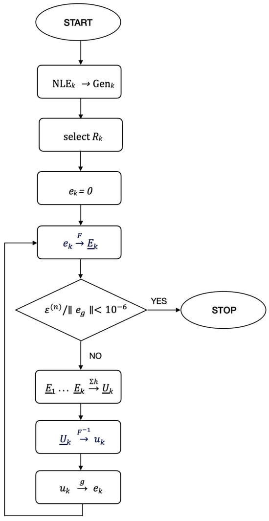
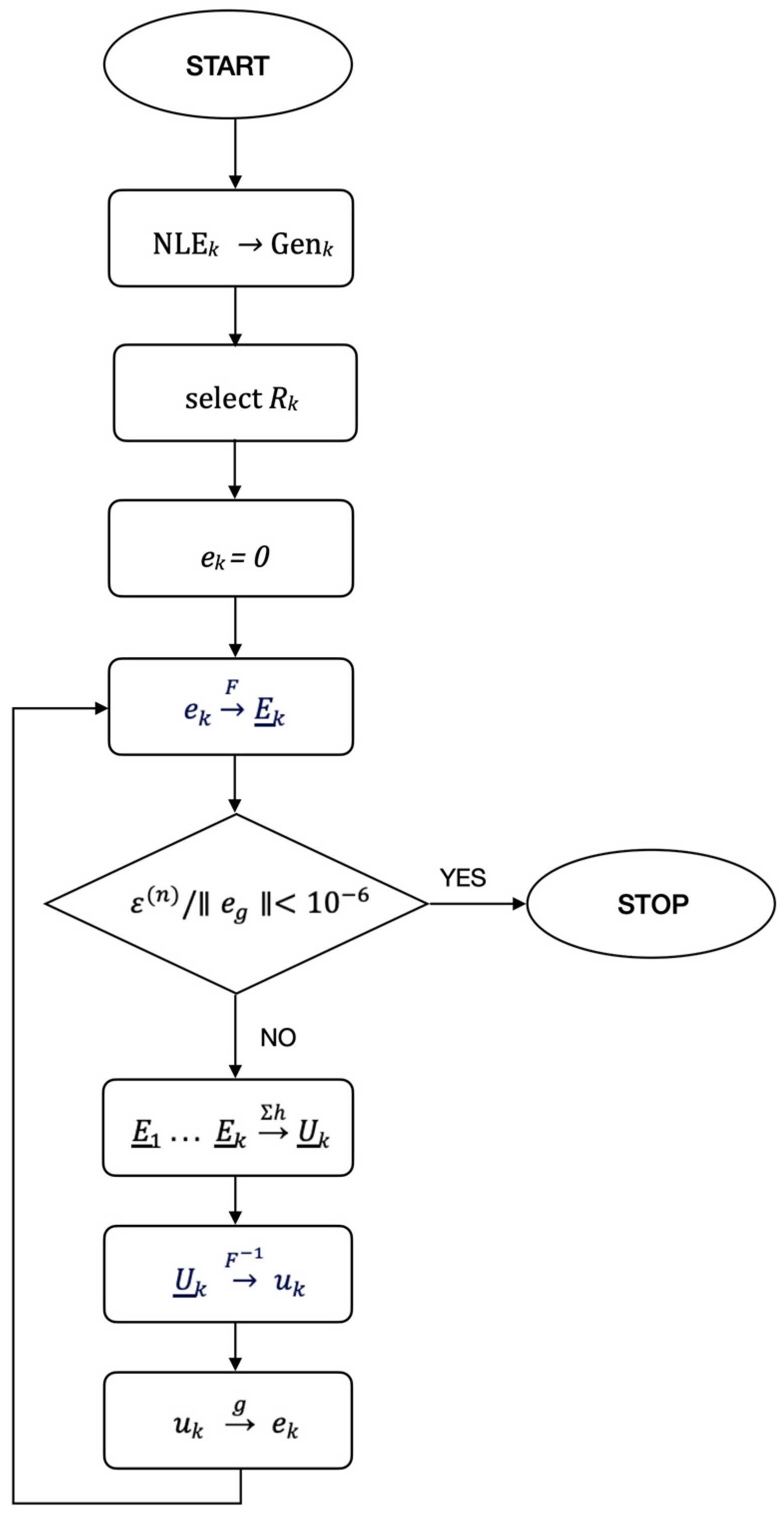
where is the source voltage of the nonlinear source , whose value is to be calculated in the time domain. is the vector of complex harmonic values of source obtained using the Fourier series expansion of and its truncation—an operation denoted by . is the frequency-domain voltage across the terminals of the generator that replaced the NLE , while is the corresponding time-domain voltage. is the inverse operation of , returning to the time domain. represents the harmonic solution of the linear circuit and the computation of the voltage at the terminals of the generator , based on the values of the sources in the circuit: the initial power sources (values kept constant during the iterations) and the nonlinear sources computed in the previous step. The circuit to be solved is linear and can be analyzed per harmonic using the superposition principle. The operator performs the correction using the nonlinear characteristic of the element in the time domain, and is the iteration number. The algorithm flowchart is presented in Figure 1.
Figure 1.
HM algorithm flowchart.
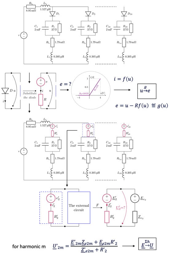
The difference between analyzing a circuit with a single NLE versus one with multiple nonlinear elements appears in the operator. The voltage at the generator terminals replacing an NLE depends not only on the pre-existing sources in the circuit and on the generator’s own nonlinear source, but also on the nonlinear sources of the other generators that replaced the other nonlinear elements in the circuit [24,25,26]. The transfer characteristics from the voltage of each nonlinear source to the voltage of the nonlinear generators involved in the calculation of are computed only once at the beginning. At each iteration, these precomputed transfer characteristics are applied to the nonlinear sources’ frequency-domain values obtained in the previous step, and the results are summed using the superposition theorem.
In practice, the equivalent generator is calculated in the frequency domain at the terminals of each NLE. At this stage, the circuit consists of linear elements and nonlinear sources, which can be easily analyzed harmonic by harmonic. The key difference when dealing with multiple nonlinearities is that the calculation for each element accounts for the contributions of all other nonlinear generators that replace the remaining nonlinear elements.
Because the analysis decomposes into separate linear problems for each frequency component, the superposition theorem enables a direct and efficient solution. Regardless of the circuit’s complexity or the number of components (linear or nonlinear), an equivalent generator is ultimately determined in the frequency domain at the terminals of each nonlinear generator. Furthermore, the transfer characteristics are computed only once during the preprocessing stage, which represents one of the primary advantages of HM.
By shifting the nonlinearities into the source, only linear circuits need to be solved in the frequency domain [23,24,25,26]. Regardless of the topology’s complexity, the equivalent voltage or current generator can be determined very quickly using existing simulation tools (e.g., via Modified Nodal Analysis based on Kirchhoff’s laws). The correction involving the nonlinear characteristic is performed exclusively in the time domain, which is computationally efficient and requires minimal effort.
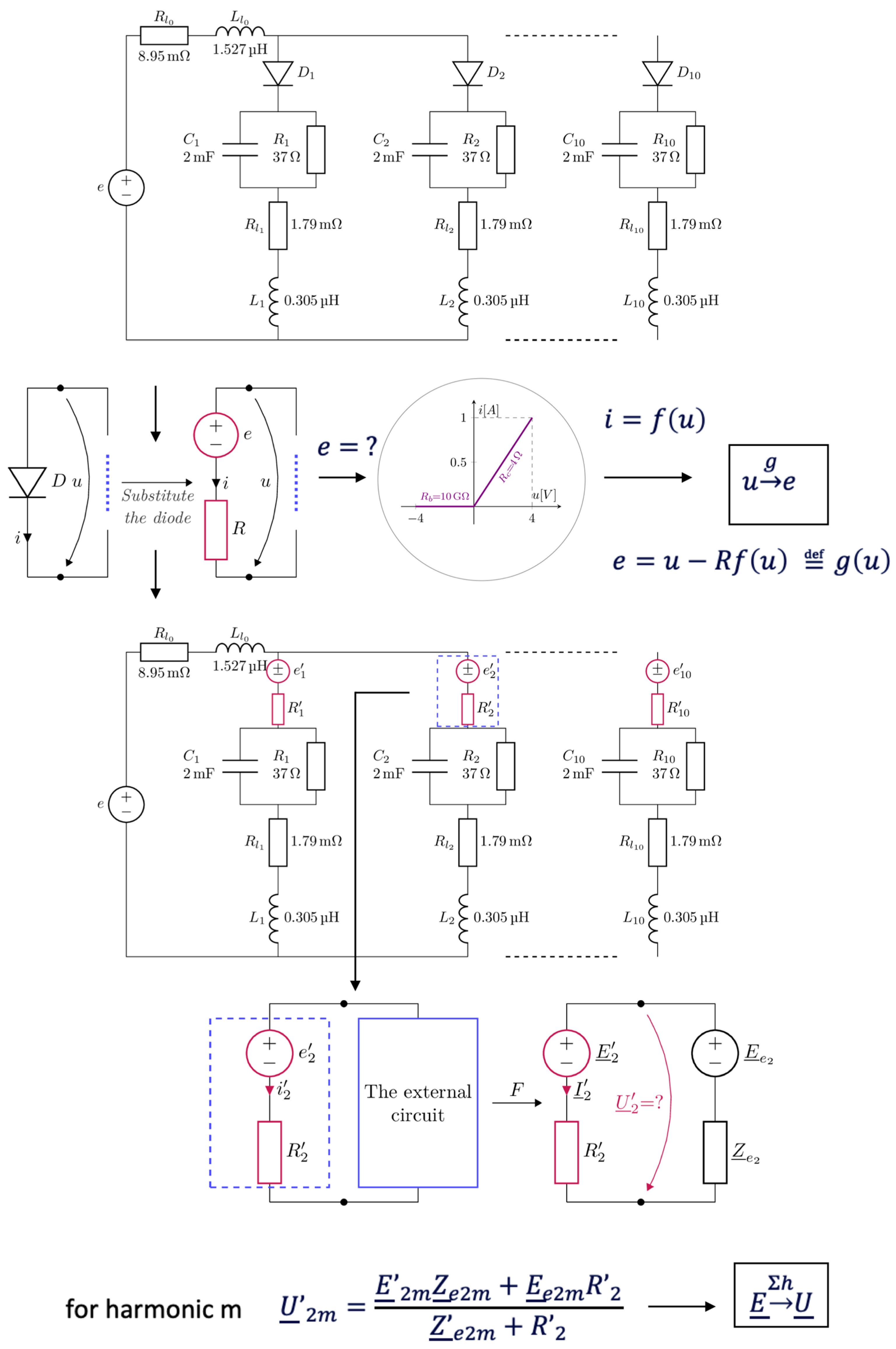
The substitution of nonlinear elements with voltage generators and the computation of the and operators are presented in Figure 2.
Figure 2.
The substitution of nonlinear elements with voltage generators and the computation of the and operators.
For the algorithm to converge, at least one of the operators , , and in (1) must be a contraction, while the others must be non-expansive [23,24,25,26]. The procedure for choosing the internal resistances of the nonlinear generators to ensure that is a contraction, as well as the non-expansive nature of the Fourier series expansion and truncation, have been discussed in detail in our previous work [23,24,25,26]. A sufficient condition for to be a contraction is that —the characteristic function of the NLE in the time domain is Lipschitz continuous and uniformly monotonic [23,24,25,26]. This leads to
and .
For the nonlinear elements typically encountered, satisfies these conditions because they operate within a finite range of voltages and currents. Consequently, the ratio between voltage and current has defined maximum and minimum values, meaning their resistance remains between a maximum value and a minimum value [23,24,25,26].
The characteristic of the NLE is . The generator replacing the NLE follows the constitutive equation . From this we define [23,24,25,26]
, the resistance of the generator that replaces the NLE is selected such that is a contraction in the Hilbert space of periodic functions. The contraction factor must exist to ensure the inequality
∀ , . The valid interval for to ensure this inequality is [16,23,24,25,26].
It remains to be established whether is still non-expansive for circuits containing multiple nonlinear elements. The proof that is non-expansive, and that truncating the Fourier series can even render it a contraction, is similar to that presented in [23,24,25,26]. For each harmonic , at the terminals of each generator (with source component and internal resistance ), we can compute the equivalent generator comprising the source and the equivalent impedance . We then compute the voltage at the terminals of the equivalent generator at harmonic :
from which it follows that the condition for to be non-expansive is satisfied:
We define the error (distance) for a source as the norm of the difference between two successive frequency-domain values of the nonlinear source [23,24,25,26]:
which is computed for all nonlinear sources .
We define the error of the algorithm at iteration as:
where is the number of nonlinear elements in the circuit.
As the stopping criterion for the iterations, we are using the relative error , where represents the amplitude of the circuit supply voltage.
After the values of the nonlinear sources in the frequency domain have been computed to the desired accuracy, the currents and voltages for all circuit elements in the frequency domain can be easily determined [23,24,25,26].
Since the algorithm is based on a Picard–Banach sequence, convergence toward the fixed point—representing the circuit solution—is always guaranteed. Unlike Newton–Raphson (NR) methods, which are prone to diverging under certain conditions, the HM provides superior numerical robustness.
In summary, HM generates a convergent Picard–Banach sequence according to Equation (1). We start with the time-domain values of the sources of the nonlinear generators (the initial value can be set to zero). Applying the Fourier series expansion, the source values in the frequency domain are obtained. The series is truncated to the desired number of harmonics.
With all source values known, together with the initial circuit sources, the circuit is solved for each harmonic, and the voltages at the terminals of all generators are obtained. The values are then converted to the time domain. For each NLE, having the value , the correction based on the nonlinear characteristic is applied in the time domain, yielding a new set of nonlinear source values. The algorithm is then repeated from the beginning until the desired relative error is reached.
3. Illustrative Example
The computational efficiency and accuracy of the proposed HM algorithm (Figure 1 and Figure 2) are benchmarked against ADS simulations. The comparison includes both the frequency-domain HB and time-domain TR solvers provided by ADS.
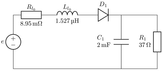
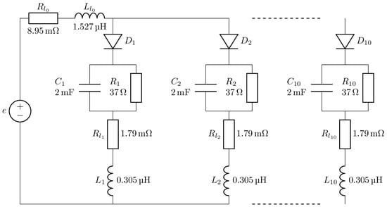
We analyzed the circuits proposed in [4] using the HM with voltage correction, considering the single half-wave rectifier configuration shown in Figure 3, the configuration with two identical parallel-connected rectifiers shown in Figure 4, and the configuration with ten identical rectifiers in parallel.
Figure 3.
Single-phase half-wave rectifier.
Figure 4.
A total of 2, respectively 10, single-phase half-wave rectifiers connected in parallel.
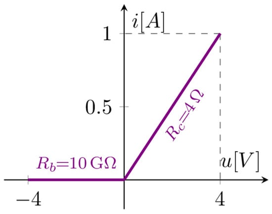
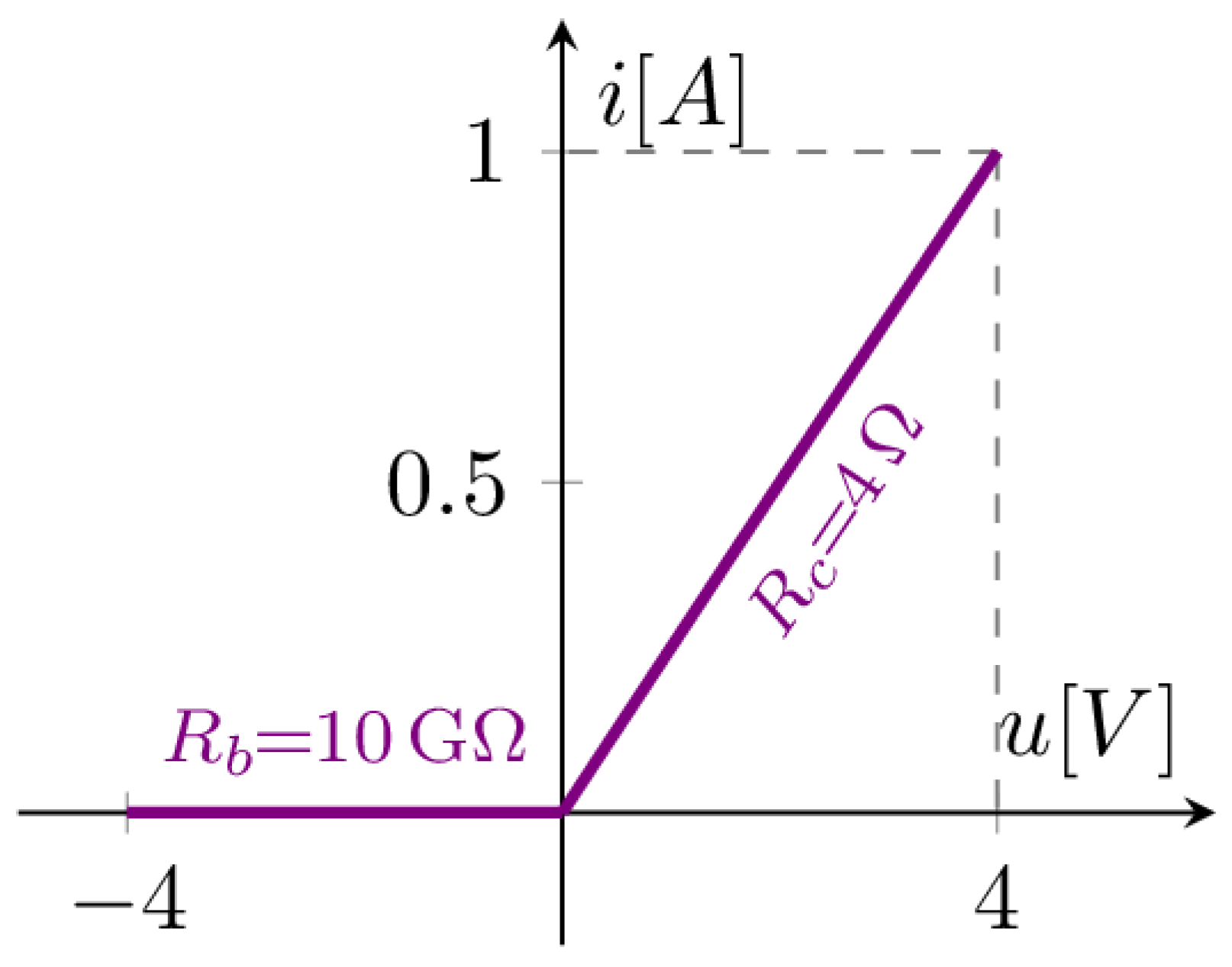
The supply source is sinusoidal, with an amplitude of 325 V, a frequency of 50 Hz, and an initial phase of 0 degrees. The nonlinear diode characteristics from [4] were approximated using a two-segment piecewise-linear model, defined by the conduction resistance and blocking resistance . The nonlinear characteristic is very steep, with a very large ratio .
The nonlinear characteristic shown in Figure 5 was applied to both the diode in Figure 3 and the diodes in Figure 4. As noted in [4], the multi-rectifier circuits include additional interconnecting conductors for parallel coupling, distinguishing them from the single-rectifier configuration. We opted to simulate the circuits exactly as presented in [4]. For this reason, the single-rectifier circuit from Figure 3 was not integrated into the unified schematic shown in Figure 4.
Figure 5.
The nonlinear diode characteristics.
Future work will extend the model to a multi-segment piecewise-linear characteristic with an added exponential section. However, computation times are not expected to increase significantly. The nonlinear characteristic correction is performed in the time domain and is very fast—on the order of 10 μs.
The Fourier series was truncated to 9, 20, 40, and 100 harmonics, plus the DC component (denoted as 9+1, 20+1, 40+1, and 100+1). Simulations for the HM were performed in GNU Octave 6.2.0 [27] using a software tool developed by the authors based on the algorithm and flowchart presented in Figure 1 and Figure 2. We used a laptop equipped with a 2.3 GHz 8-Core Intel Core i9 processor (9th Generation) and 16 GB 2667 MHz DDR4 memory. Table 1 summarizes the computation times in milliseconds, the required number of iterations, and the number of sampling points per period. Convergence was assumed when the relative error reached . The analysis employed the original HM algorithm [16,17,18,19,20,21,22,23,24,25] rather than the modified version from [26].
Table 1.
Computation times and number of iterations for various configurations using HM.
No specific acceleration techniques presented in [23,24,25,26] were used, as they were unnecessary. The calculations used optimal internal resistances which inherently improve the method’s convergence rate [23,24,25,26]. Notably, the inclusion of the equivalent resistance calculated at the NLE terminals [24] could be easily implemented to further minimize computation time. If higher computation speed is desired, the number of harmonics, the number of sampling points, or the relative error can be reduced. Conversely, if higher accuracy is required, these parameters can be increased. Additionally, acceleration techniques [21,22,23,24,25] or the modified algorithm [26] can be applied to enhance performance, demonstrating the method’s versatility.
The analysis accounted for existing circuit symmetries and the identical nature of the nonlinear characteristics. The correction using the nonlinear characteristic and the application of the operators and were performed only once per iteration, resulting in a significant time saving. If the nonlinear characteristics differed for each rectifier, these operations would be required for each element individually. In the worst-case scenario, the computation time would scale linearly with the number of rectifiers. This case will be addressed in a future study.
Table 2 presents the computation times obtained with ADS 2026 [28] using the HB method for the same circuits and diode characteristics. The Fourier series truncation and the number of samples per period were kept the same for consistency.
Table 2.
Computation times for ADS 2026 [28] using HB.
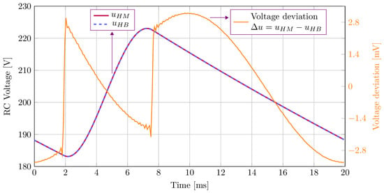
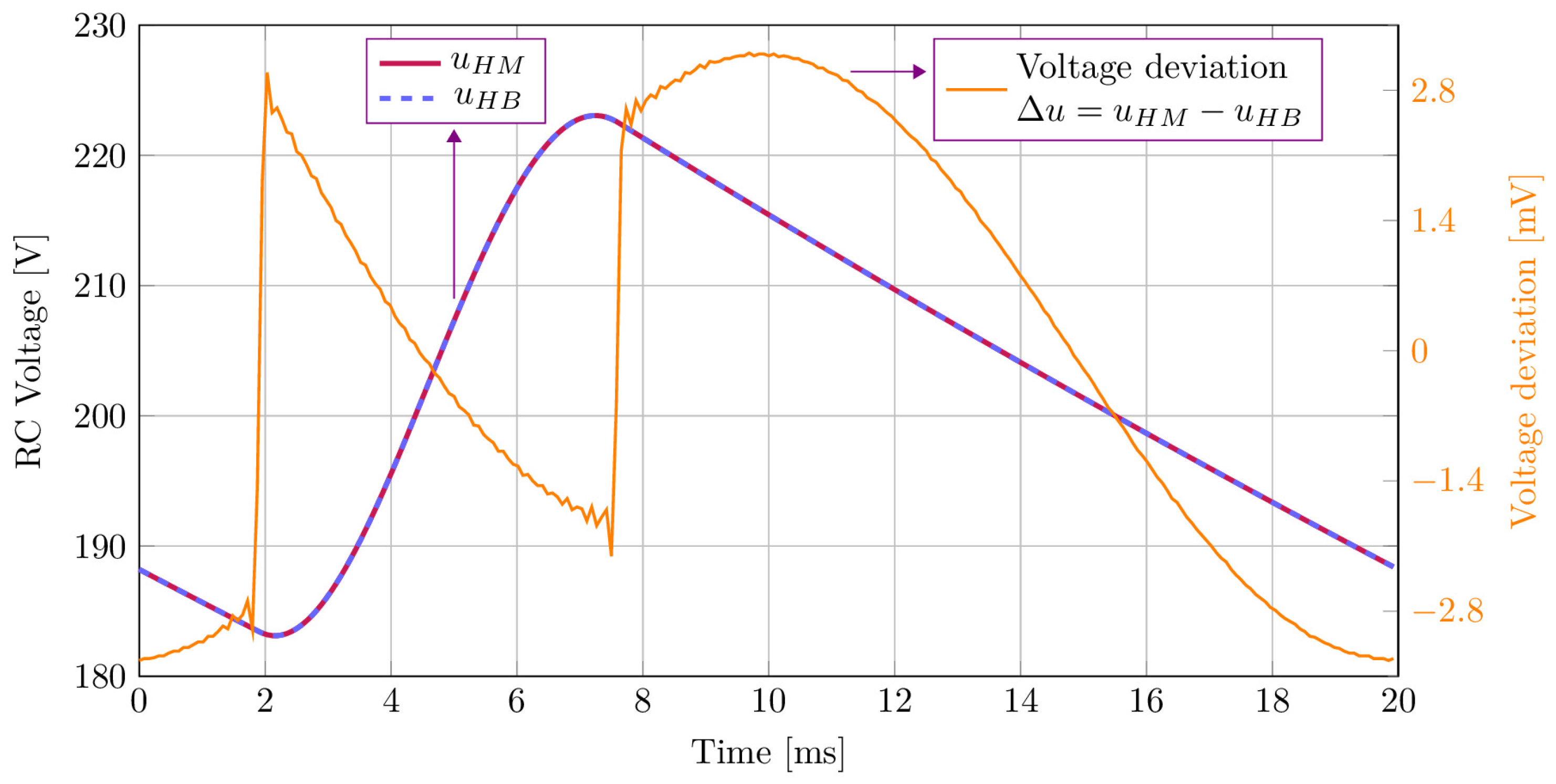
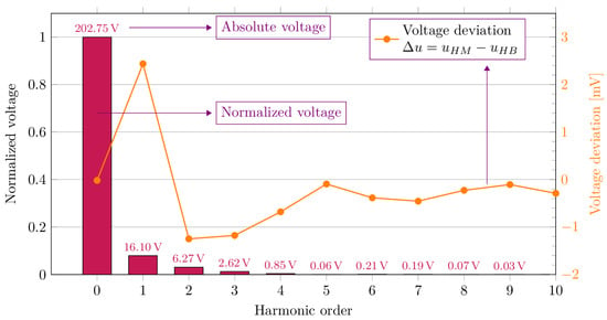
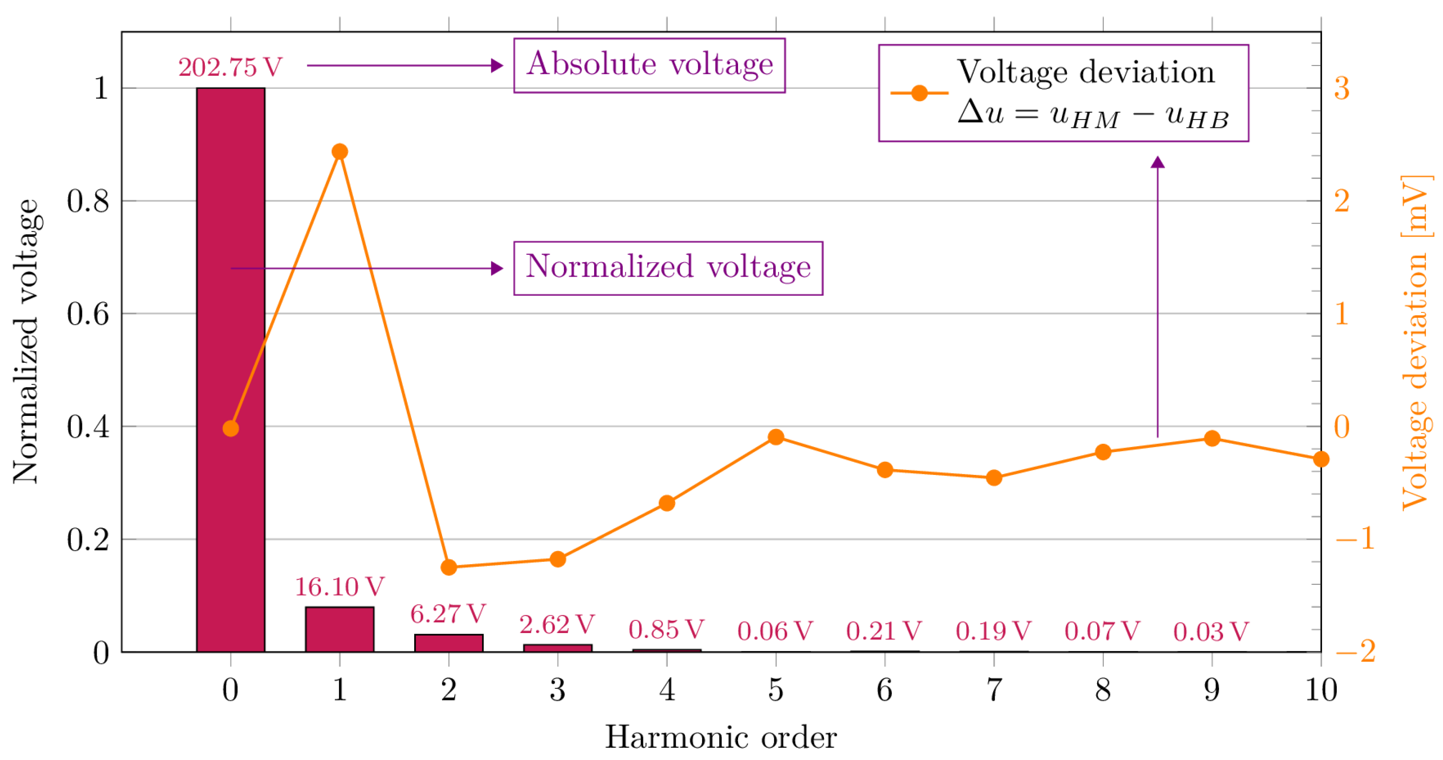
Figure 6, Figure 7 and Figure 8 present a comparative view of the RC load voltage and its harmonic spectrum (peak values) for the 10-rectifier case, computed using 100+1 harmonics and 256 sampling points. The harmonic amplitudes are small except for the DC component. However, the second and third harmonics remain significant. Methods that neglect even or triplen harmonics may yield incorrect results in such cases. The absence of higher-order harmonics was expected, given the rectifier’s low-pass filter configuration (Figure 3).
Figure 6.
RC voltage and deviation for 10 rectifiers: HM vs. ADS HB results with 100+1 harmonics.
Figure 7.
Harmonic spectrum of the RC voltage (peak values and % of the DC component) and deviation for 10 rectifiers HM vs. ADS HB results with 100+1 harmonics.
Figure 8.
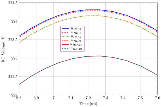
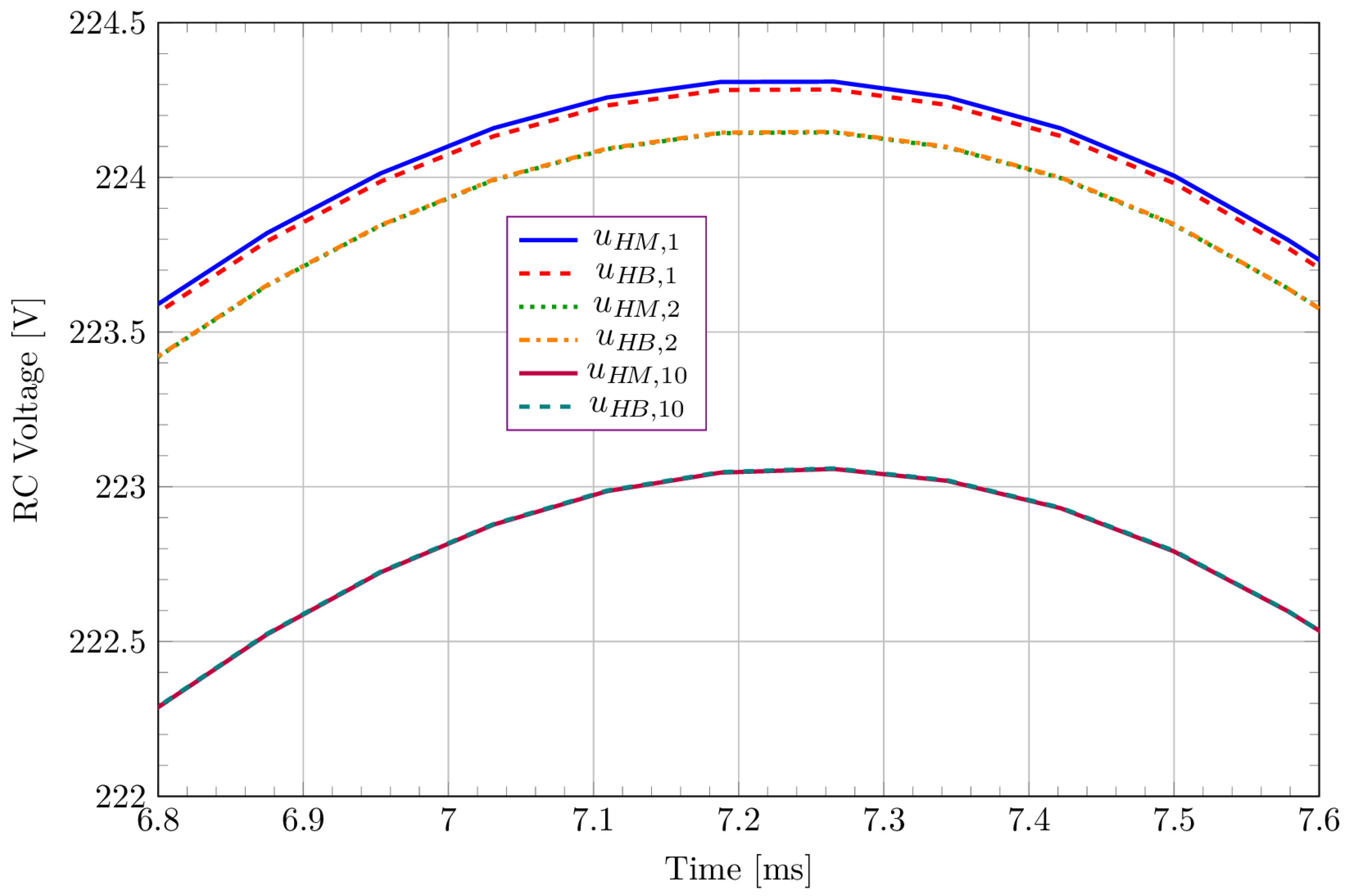
Detailed view of superimposed RC voltage waveforms for 1, 2, and 10 rectifiers HM vs. ADS HB results with 100+1 harmonics.
Figure 8 shows a superimposed detail of the RC voltage for 1-, 2-, and 10-rectifier circuits. An expected voltage drop is observed as the number of parallel-connected rectifiers increases. The HM results are validated by the HB results. The relative deviation between the two methods for the RC voltage (Figure 6), defined as , does not exceed 1.8 × 10⁻⁵.
TR in ADS can detect the time at which the steady state is reached, which occurs at time t = 140 ms for the circuits studied in this article. To obtain the solution (waveform) closer to those obtained with HM and HB, it was necessary to increase the final simulation time to Tstop = 260 ms. With these settings, the voltage deviation for the solutions given by HB and the TR over a period ( for the TR) for the RC Voltage does not exceed 5.5 mV.
In TR, the time step can be set either automatically by the simulator or manually by the user. To compare the computational time with that obtained using HM and HB, we imposed the same number of samples over a time period as in the previously mentioned methods. The results are presented in Table 3.
Table 3.
Computation times for ADS 2026 [28] using TR.
If we select the steady-state detection and let the program choose the time step, depending on the integration method (trap or gear of order 2 to 6), the steady-state solution is reached at a later time (190 ms to 210 ms).
In the current GNU Octave [27] implementation for HM, the transfer characteristics for the operator were derived analytically, while the program performed only the numerical computations. Ongoing development aims to integrate a SPICE module to automatically analyze the circuit and compute transfer characteristics for any user-defined topology.
For the and operators, the classical Fourier series expansion and its inverse transformation were used. The coefficients were computed once during the preprocessing stage. The period was divided into equal intervals, assuming a linear approximation of the signal between points, allowing for analytical calculation of the integrals. To reduce floating-point errors, the arguments of sine and cosine were mapped to the first quadrant [23,24,25,26]. All preprocessing operations are included in the total computation time.
Standard FFT and IFFT routines available in GNU Octave, as used in ADS, were not utilized. While the method supports FFT/IFFT, these routines can be unreliable under certain conditions, such as abrupt signal variations caused by resonances or controlled switching elements (e.g., thyristors) [21,22,23,24,25,26]. In [24], using FFT/IFFT significantly increased the number of iterations required to reach the target error, despite reducing the time per iteration. Although the chosen analytical approach is slower, it offers superior precision, versatility, and robustness for any circuit type. For simple circuits with few significant harmonics, FFT/IFFT could potentially lead to further reductions in computation time.
It is worth noting that ADS—whether operating in the frequency or time domain—handles nonlinearities using NR. While NR is characterized by quadratic convergence and is renowned for its speed, it is also prone to convergence issues. Despite a reduction in the number of iterations in the case of ADS, the overall computational time remains significant.
The method is versatile, enabling a trade-off between computational speed and high precision depending on the application. By reducing the number of analyzed harmonics or sampling points, or by increasing the convergence threshold, computation time can be further minimized. Conversely, higher accuracy is attainable by increasing these parameters. For the analyzed circuits, the number of significant harmonics is very small (up to the 4th harmonic). Therefore, good accuracy can be achieved with short computation times. The results obtained with 20+1 or even 9+1 harmonics are sufficiently accurate, even when using a small number of sampling points per period. Even without exploiting circuit symmetry, in the worst-case scenario, computation time would scale linearly with the number of rectifiers while remaining computationally inexpensive.
The HM requires minimal computational effort. The transfer characteristics, determined by the linear part of the circuit connected to the NLE terminals, are computed only once at the beginning. The correction using the nonlinear characteristic is performed in the time domain and is extremely fast. The most time-consuming operations are the Fourier series expansion and the subsequent inverse transformation to the time domain. When truncated to a small number of harmonics (under 100) and a reduced number of sampling points (under 1000), the computational effort is minimal and the computation time is very short, even on standard computing hardware. Since the method is based on an iterative procedure, there is no need to solve complex systems of nonlinear equations [23,24,25,26]. Only a single system of linear equations is solved initially to calculate the transfer characteristics, which are then reused throughout the iterations.
4. Conclusions
The results presented in this paper demonstrate that the HM is very fast. It outperforms conventional computation methods implemented in commercial software. This performance is achieved without employing acceleration techniques or modified algorithms. The method remains efficient regardless of the presence of highly nonlinear (steep) characteristics. It is effective for solving NRCEs and enables fast and accurate evaluation of harmonic distortion.
The advantages of the method include guaranteed, mathematically proven convergence, as well as low computational effort and time. The method can also achieve high precision by using a large number of harmonics and sampling points, without the need to forcibly eliminate even or triplen harmonics.
It is worth noting that the HM has successfully solved specific NRCEs that other methods failed to address. This includes three-phase nonlinear configurations, harmonic resonances, and circuits with distinct sequence reactances. Furthermore, it addresses controlled switching elements, such as thyristors, and abrupt signal variations prone to the Gibbs phenomenon. The method handles combinations of these phenomena while simultaneously allowing the analysis of a large number of harmonics within a reasonable computation time [23,24,25,26].
To date, no significant flaws have been observed regarding the HM. For specific scenarios where performance might deteriorate, the acceleration techniques developed in our previous papers [24,25,26] have been successfully implemented to address such limitations. However, this was not necessary for the circuits analyzed in the present article.
Future research will focus on full-wave rectifiers and nonlinear elements modeled with more complex piecewise-linear approximations, supplemented by an exponential section.
In future work, we intend to conduct a comparative analysis of the HM against ADS and other commercial software packages for more complex topologies and circuits with a higher number of linear and nonlinear elements, including experimental validation using laboratory-measured data. It should be noted that the results obtained in our previous studies [24,25,26] have already been validated through time-domain simulations performed in LTspice [29].
Furthermore, we aim to compare the HM with other computational and numerical methods proposed in the literature, and we welcome research collaborations in this field. Our objective is to demonstrate that the HM has the attributes and advantages needed for integration into commercial circuit simulation software. This may include developing a dedicated add-on module for existing open-source, freeware, or proprietary simulation platforms.
Author Contributions
Conceptualization, C.T., A.G.G. and G.M.V.; methodology, C.T., A.G.G. and G.M.V.; software, C.T., A.G.G. and G.M.V.; validation, C.T., A.G.G. and G.M.V.; formal analysis, C.T., A.G.G. and G.M.V.; investigation, C.T., A.G.G. and G.M.V.; resources, C.T., A.G.G. and G.M.V.; data curation, C.T., A.G.G. and G.M.V.; writing—original draft preparation, C.T., A.G.G. and G.M.V.; writing—review and editing, C.T., A.G.G. and G.M.V.; visualization, C.T., A.G.G. and G.M.V.; supervision, C.T., A.G.G. and G.M.V.; project administration, C.T.; funding acquisition, C.T., A.G.G. and G.M.V. All authors have read and agreed to the published version of the manuscript.
Funding
This research received no external funding.
Data Availability Statement
The original contributions presented in this study are included in the article. Further inquiries can be directed to the corresponding author.
Acknowledgments
We would like to thank Florin Constantinescu for the extremely helpful discussions and for his persistence in performing the simulations presented in this article.
Conflicts of Interest
The authors declare no conflicts of interest.
Abbreviations
The following abbreviations are used in this manuscript:
| HM | Hănțilă Method |
| HB | Harmonic Balance |
| TR | Transient Analysis |
| NR | Newton–Raphson |
| NRCEs | Circuits with Multiple Nonlinear Resistive Elements |
| NRCE | Circuits with One Nonlinear Resistive Element |
| NLE | Nonlinear Element |
| DC | Direct Current |
| RC | Resistor–Capacitor |
| Gen | Generator |
| ADS | Advanced Design System |
| FFT | Fast Fourier Transform |
| IFFT | Inverse Fast Fourier Transform |
References
- Wcislik, M.; Kazala, R.; Strzabala, P. Characteristics and Parameters of a Three-Phase, Three-Wire Balanced Circuit with Non-Linear Load. Energies 2024, 17, 1867. [Google Scholar] [CrossRef] [Scilit]
- Choi, J.; Bak, Y. Double Fourier Series-Based Sideband Harmonic Analysis of a Full-Bridge Converter. Mathematics 2026, 14, 617. [Google Scholar] [CrossRef] [Scilit]
- Albalawi, H.; Wadood, A.; Khan, S.; Alatwi, A.M. Harmonic Mitigation in Multi-Pulse Rectification: A Comparative Study of 12-, 18-, and 24-Pulse Systems. Mathematics 2024, 12, 3257. [Google Scholar] [CrossRef] [Scilit]
- Constantinescu, F.; Gheorghe, A.; Barancea, C.G. Efficient Frequency Domain Models for Simulation of Circuits with Diode Rectifiers. In Proceedings of the International Symposium on Fundamentals of Electrical Engineering (ISFEE), Bucharest, Romania, 16–18 November 2023; pp. 1–6. [Google Scholar] [CrossRef] [Scilit]
- Azab, M. Low-Cost Active Power Filter Using Four-Switch Three-Phase Inverter Scheme. Electricity 2025, 6, 16. [Google Scholar] [CrossRef] [Scilit]
- Aravanis, T.; Papadopoulos, P.; Georgikos, D. Fourier Feature-Enhanced Neural Networks for Wind Turbine Power Modeling. Electricity 2025, 6, 70. [Google Scholar] [CrossRef] [Scilit]
- Hidalgo Monsivais, L.C.; León Ruiz, Y.; Hernández Ramírez, J.C.; Visairo-Cruz, N.; Segundo-Ramírez, J.; Barocio, E. Controller Hardware-in-the-Loop Validation of a DSP-Controlled Grid-Tied Inverter Using Impedance and Time-Domain Approaches. Electricity 2025, 6, 52. [Google Scholar] [CrossRef] [Scilit]
- Li, Q.; Wang, Y.; Mao, T. Loss Prediction and Global Sensitivity Analysis for Distribution Transformers Based on NRBO-Transformer-BiLSTM. Electronics 2026, 15, 420. [Google Scholar] [CrossRef] [Scilit]
- Liang, P.; Pei, X.; Zhou, Y.; Wu, H.; Xu, Y.; Zhang, Z.; Xu, Z.; Qiu, F. Harmonic Analysis and Elimination of Transmission Scheme Based on DRU for Medium-Frequency Offshore Wind Farms. Electronics 2025, 14, 3669. [Google Scholar] [CrossRef] [Scilit]
- Yumurtacı, R.; Terkeş, M.; Demirci, A.; Tercan, S.M. A detailed framework for modeling three-phase power system components in phase coordinates at harmonic frequencies. In Proceedings of the 12th International Artemis Scientific Research Congress, București, Romania, 28–30 May 2025; Volume 1, pp. 1–10. [Google Scholar]
- Ştefănescu, V.; Hathazi, F.I.; Raţă, G.; Ungureanu, C. Technical losses caused by poor power quality in electrical networks with nonlinear consumers. Rev. Roum. Sci. Techn.–Électrotechn. Énerg. 2025, 70, 337–342. [Google Scholar] [CrossRef] [Scilit]
- Panoiu, M.; Ivascanu, P.; Panoiu, C. Analysis of Operating Regimes and THD Forecasting in Steelmaking Plant Power Systems Using Advanced Neural Architectures. Mathematics 2025, 13, 3692. [Google Scholar] [CrossRef] [Scilit]
- Li, Y.; Wang, X. Modeling and Simulation of a PINN-Based Nonlinear Motor Drive System. Appl. Sci. 2026, 16, 3426. [Google Scholar] [CrossRef] [Scilit]
- Rong, S.; Lei, X.; Meng, F.; Gu, B.; Mu, Z.; Cui, J.; Ye, K.; Yong, S.; Zhang, P.; Guan, J. Triple-Passive Harmonic Suppression Method for Delta-Connected Rectifier to Reduce the Harmonic Content on the Grid Side. Appl. Sci. 2025, 15, 13282. [Google Scholar] [CrossRef] [Scilit]
- Deliu, A.D.; Cazacu, E.; Deliu, F.; Popa, C.; Popa, N.S.; Preda, M. Dynamic Average-Value Modeling and Stability of Shipboard PV–Battery Converters with Curve-Scanning Global MPPT. Electricity 2025, 6, 66. [Google Scholar] [CrossRef] [Scilit]
- Hantila, I.F. A method for solving nonlinear resistive networks. Rev. Roum. Sci. Techn.–Électrotechn. Énerg. 1979, 24, 217–226. [Google Scholar]
- Hantila, I.F.; Preda, G.; Vasiliu, M. Polarization method for static fields. IEEE Trans. Magn. 2000, 36, 672–675. [Google Scholar] [CrossRef] [Scilit]
- Ciric, I.; Hantila, F. An efficient harmonic method for solving nonlinear time-periodic eddy-current problems. IEEE Trans. Magn. 2007, 43, 1185–1188. [Google Scholar] [CrossRef]
- Hantila, I.F. A method for solving stationary magnetic field in nonlinear media. Rev. Roum. Sci. Techn.–Électrotechn. Énerg. 1975, 20, 397–407. [Google Scholar]
- Preda, G.; Cranganu-Cretu, B.; Hantila, F.I.; Mihalache, O.; Chen, Z.; Miya, K. Nonlinear FEM–BEM Formulation and Model-Free Inversion Procedure for Reconstruction of Cracks Using Pulse Eddy Currents. IEEE Trans. Magn. 2002, 38, 1241–1244. [Google Scholar] [CrossRef]
- Albanese, R.; Hantila, F.I.; Rubinacci, G. A nonlinear eddy current integral formulation in terms of a two-component current density vector potential. IEEE Trans. Magn. 1996, 32, 784–787. [Google Scholar] [CrossRef] [Scilit]
- Albanese, R.; Hantila, F.I.; Preda, G.; Rubinacci, G. A Nonlinear Eddy-Current Integral Formulation for Moving Bodies. IEEE Trans. Magn. 1998, 34, 2529–2532. [Google Scholar] [CrossRef] [Scilit]
- Hantila, I.F.; Maricaru, M.; Ciuceanu, R.M.; Corlan, L. Harmonic analysis of circuits with nonlinear resistive elements. Rev. Roum. Sci. Techn.–Électrotechn. Énerg. 2012, 57, 333–340. [Google Scholar]
- Tufan, C.; Maricaru, M.; Nemoianu, I.V. Procedures for accelerating the convergence of the Hantila method for solving three-phase circuits with nonlinear elements—Part II. Rev. Roum. Sci. Techn.–Électrotechn. Énerg. 2022, 67, 395–401. [Google Scholar]
- Tufan, C.; Marin, M.E.; Vasilescu, G.M.; Ciuceanu, M.R.; Maricaru, M. Dynamic relaxation in the iterative methods for solving nonlinear three-phase circuits. Rev. Roum. Sci. Techn.–Électrotechn. Énerg. 2023, 68, 289–294. [Google Scholar] [CrossRef] [Scilit]
- Tufan, C.; Vasilescu, G.M.; Hănţilă, I.F.; Bordianu, A.; Maricaru, M. A Faster Algorithm for Frequency Solving of Nonlinear Three-Phase Circuits. In Proceedings of the International Symposium on Fundamentals of Electrical Engineering (ISFEE), Bucharest, Romania, 16–18 November 2023; pp. 1–4. [Google Scholar] [CrossRef] [Scilit]
- GNU Octave. Available online: https://octave.org (accessed on 15 January 2026).
- Keysight Technologies. PathWave Advanced Design System (ADS). Available online: https://www.keysight.com/us/en/lib/software-detail/computer-software/pathwave-advanced-design-system-ads-software-2212036.html (accessed on 15 January 2026).
- LTspice. Available online: https://www.analog.com/en/resources/design-tools-and-calculators/ltspice-simulator.html (accessed on 15 January 2026).

Disclaimer/Publisher’s Note: The statements, opinions and data contained in all publications are solely those of the individual author(s) and contributor(s) and not of MDPI and/or the editor(s). MDPI and/or the editor(s) disclaim responsibility for any injury to people or property resulting from any ideas, methods, instructions or products referred to in the content. |
© 2026 by the authors. Licensee MDPI, Basel, Switzerland. This article is an open access article distributed under the terms and conditions of the Creative Commons Attribution (CC BY) license.