


Abstract
The mathematical characterization of non-stationary signals remains a significant challenge, particularly when impulsive components are obscured by high-dimensional noise and structural coupling. This paper proposes an application-driven mathematical methodology for a learnable discrete wavelet transform (LDWT) that combines classical multi-resolution analysis with task-optimized data-driven adaptivity. Rather than introducing entirely new foundational theory, our approach strategically relaxes constraints from orthogonal wavelet theory within the non-perfect reconstruction filter bank framework, enabling controlled spectral decomposition optimized for supervised fault diagnosis. We introduce a specialized regularization term based on the half-band property to ensure spectral complementarity and minimize cross-band correlation, while a Jacobian-based stabilization approach is formulated to ensure the convergence of filter coefficients during optimization. The proposed algorithmic architecture, LDBRFnet, features a dual-branch encoder system designed to capture the mathematical synergy between sub-band-level global statistics and time-domain local morphology. This dual-view representation effectively mitigates feature leakage and overconfidence in classification. Theoretical analysis and numerical experiments demonstrate that the learned filters satisfy the frequency-shift property and maintain robust spectral partitioning even under low signal-to-noise ratios. Validation on complex vibration datasets confirms that the framework achieves superior diagnostic accuracy (over 95.5%) and computational efficiency, reducing model parameters by 96.7% compared to state-of-the-art baselines. This work provides a generalizable mathematical approach for adaptive signal decomposition and robust pattern recognition in interdisciplinary applications.
Keywords:
multiresolution analysis; learnable wavelet transform; quadrature mirror filters; non-stationary signal processing; inductive bias; adaptive feature extraction; spectral complementarity MSC:
42C15; 94A12; 68T07
1. Introduction
Rolling bearing fault diagnosis faces significant challenges due to the non-stationary nature of vibration signals, which contain weak impulsive components often obscured by measurement noise and structural coupling [1,2,3]. Traditional signal processing approaches relying on Fourier transforms or wavelet analysis require manual parameter tuning and struggle with variable operating conditions [4,5,6]. While deep learning methods have shown promise in automated feature extraction [7,8,9], they remain sensitive to noise statistics and normalization procedures, often producing overconfident predictions in imbalanced datasets [10].
Wavelet-based techniques have demonstrated advantages in time–frequency localization for non-stationary signals [11]. Variants like variational mode decomposition (VMD) and empirical mode decomposition (EMD) can isolate fault-related components [12], but their performance depends heavily on parameter selection and suffers from mode mixing effects [13,14]. Recent hybrid approaches combining signal processing with deep learning have improved robustness [15], yet challenges persist in maintaining consistent performance across different signal-to-noise ratios and operating conditions [16,17].
Learnable wavelet transforms have recently been leveraged to address the limitations of fixed, hand-crafted wavelet bases in capturing non-stationary signal characteristics. By parameterizing wavelet decomposition through trainable quadrature mirror filters or learnable multi-scale Haar modules, these methods can adapt the time–frequency representation to the data end-to-end, improving robustness under noise and enhancing interpretability compared with purely convolutional or self-attention-based alternatives. Building on this line of work, we introduce an LDWT frontend with a physically interpretable filter construction and integrate it into a dual-branch architecture for noise-robust bearing fault diagnosis [18,19,20,21].
The limitations of current methods become particularly apparent when dealing with early-stage faults exhibiting weak signatures [22]. Most approaches focus either on time-domain or frequency-domain features, lacking comprehensive multi-scale characterization [23,24]. Attention mechanisms and transformer architectures have been employed to capture long-range dependencies [25,26], but they often fail to adequately address global noise coupling effects and inter-task conflicts [27,28].
This paper positions itself within signal processing and machine learning rather than foundational wavelet theory. Our mathematical contributions are best understood as (i) a methodological refinement of filter bank design for supervised learning, (ii) formal analysis of the stability and leakage behavior under soft constraints, and (iii) algorithmic innovations for robust feature extraction. While we do not propose entirely new axioms or theorems of fundamental importance to harmonic analysis, we provide rigorous mathematical analysis that extends the understanding of learnable decompositions for applications requiring noise robustness.
To address these challenges, we propose an end-to-end framework featuring a learnable discrete wavelet transform (LDWT) frontend with dual complementary encoders, termed LDBRFnet. The main contributions of this work are summarized as follows:
- (1)
- Learnable wavelet decomposition with methodologically refined weak QMF constraints. We propose a learnable discrete wavelet transform (LDWT) that replaces fixed wavelet bases with trainable quadrature mirror filters (QMFs) within the established non-perfect reconstruction (non-PR) filter bank framework. Soft half-band regularization is introduced to encourage spectral complementarity between low- and high-frequency sub-bands while maintaining sufficient flexibility for task-driven optimization. This methodological contribution—combining soft regularization (Theorem 1), Jacobian stabilization (Proposition 1), and learnable filter parameterization—enables interpretable and adaptive time–frequency decomposition while maintaining formal control over spectral leakage. This design improves the separability of weak impulsive fault signatures under noisy conditions.
- (2)
- Dual-branch complementary encoder architecture for decoupled fault feature extraction. A dual-branch encoder architecture is developed to capture complementary fault characteristics from the learned sub-band signals. The LDWT-Encoder branch models global sub-band statistics using a multilayer perceptron, while the ResNet1D-Encoder branch focuses on local temporal morphology through residual convolutional blocks. This dual-view representation effectively reduces feature leakage and improves robustness to sampling strategies and signal normalization.
- (3)
- Noise-robust multi-head learning framework with weighted auxiliary supervision. A weighted multi-head training strategy is designed to jointly optimize the two encoder branches. The auxiliary supervision provided by the LDWT branch enhances the stability of feature learning, while the dominant ResNet1D branch preserves discriminative temporal structures. This cooperative optimization improves robustness to noise interference and domain variations, leading to reliable fault diagnosis across different operating conditions.
While our work strategically applies classical filter bank theory and multi-task learning to fault diagnosis, the specific methodological innovations—soft half-band regularization with leakage bounds (Section 2.2.6), Jacobian-based convergence guarantees (Proposition 1), and the learnable dual-branch architecture—represent significant methodological and analytical advances that enable both rigor and adaptivity in fault diagnosis. This work is best described as an application-driven methodological contribution that achieves superior performance (95.5% average accuracy, 96.7% parameter reduction) while maintaining interpretability and mathematical formality.
The proposed method demonstrates superior performance compared to existing approaches, achieving 95.5% average accuracy in cross-domain transfer tasks while maintaining interpretability through its learnable wavelet decomposition [15]. The experimental results on multiple bearing fault datasets confirm the robustness of our approach under challenging noise conditions and variable operating scenarios [16].
2. Methodology
2.1. Overview
The proposed LDBRFnet framework integrates a learnable discrete wavelet transform (LDWT) frontend with dual-branch encoders to achieve end-to-end fault diagnosis.
As illustrated in Figure 1, the network processes input vibration signals through three key components: (1) The LDWT module performs data-adaptive sub-band decomposition to enhance impulse features, (2) the LDWT-Encoder branch extracts global sub-band statistics using MLP layers, and (3) the ResNet1D-Encoder captures local temporal patterns through 1D convolutions. We jointly optimize these complementary branches via a weighted multi-head objective, enabling synergistic learning of multi-scale fault characteristics. The architecture specifically addresses three challenges in noisy bearing diagnosis: modal aliasing through learnable wavelets, feature leakage via dual-branch constraints, and SNR sensitivity via cross-domain consistency regularization.
Figure 1.
Overall architecture of LDBRFnet.
2.2. Learnable DWT Frontend
The learnable discrete wavelet transform (DWT) frontend (Learnable-DWT), shown in Figure 2, injects multiple resolutions and time–frequency localization inductive bias through trainable orthogonal-complementary filters, preserving interpretability while enhancing adaptivity. This enables data-driven energy reallocation and sparsity promotion of impulsive components, improving SNR and separability of weak high-frequency impulses.
Figure 2.
Architecture of the Learnable-DWT module.
For an input batch , the Learnable-DWT produces:
where with stride . The design enforces spectral complementarity through quadrature mirror filter (QMF) constraints while reducing parameters via kernel sharing.
2.2.1. Filter Construction and Properties
The normalized low-pass kernel is learned with stabilization:
The high-pass filter g derives from QMF relations:
This construction ensures the frequency-shift property , proven via DTFT analysis of the anti-symmetric kernel.
2.2.2. Forward and Backward Propagation
To formalize the operators used in the Learnable-DWT frontend, we define the padding extension and the strided convolution as follows.
- Padding operator.
Let denote the discrete input signal. For an analysis filter length K, we extend x to by a boundary extension of radius . In this work, we adopt reflection padding:
Equivalently, the extended sequence is truncated to the index range required by the subsequent convolution computation.
- Strided convolution operator.
Let be a discrete filter. We define the strided convolution output by . This definition corresponds to computing a standard (discrete) convolution/correlation over the padded signal and evaluating it only at strided time indices . Here is the stride (downsampling factor).
- Downsampling operator (optional notation consistency).
For a sequence , we define as .
With the above operators, the sub-band outputs for input x are defined as
where under the adopted padding and output sampling rule.
Gradients propagate through both filters during training. Let and denote the error gradients; the total gradient w.r.t. combines direct and QMF-induced terms:
In Equation (6), the operator D denotes the linear mapping induced by the QMF-based analysis/synthesis filter parametrization. Specifically, the synthesis-side filter coefficients are obtained as a linear transform of the analysis-side coefficients through , where is the normalized prototype filter (see the normalization in Equation (17)). Consequently, holds in a linear operator form. Therefore, the gradient propagated to the g-space appears as in accordance with the chain rule (i.e., ).
Moreover, Equation (7) is derived from the Jacobian of the normalization step. Let (Equation (17)). Then follows from differentiating the above normalization, and substituting this Jacobian into the chain rule yields the form reported in Equation (7). The Jacobian of normalization ensures stable updates to the base kernel h:
where and . This formulation maintains filter orthogonality while adapting to the characteristics of the vibration signal. The Jacobian-based stabilization in Equation (6) is introduced to control the sensitivity of the normalized LDWT kernels, and its theoretical guarantee is established in Proposition 1 in Section 2.6.
2.2.3. Weakly Constrained QMF-Based Learnable Wavelet Transform
The proposed learnable discrete wavelet transform (LDWT) acts as the frontend feature extractor. Unlike conventional orthogonal and biorthogonal wavelet transforms that enforce strict orthogonality and perfect reconstruction [29,30], the LDWT adopts a weakly constrained quadrature mirror filter (QMF) coupling mechanism within the non-perfect reconstruction (non-PR) filter bank framework [31]. This design achieves spectral complementarity through soft half-band regularization while preserving flexibility for task-driven optimization, as formalized in frame theory (Section 2.2.4).
Specifically, only the low-pass prototype filter h is learned from data, while the high-pass filter is constructed through the QMF relation
where k denotes the filter length.
This design ties the two analysis branches through a mirror structure, encouraging complementary spectral partitioning while significantly reducing the parameter space.
To further promote interpretable sub-band decomposition, we employ normalization on the low-pass kernel and introduce a soft half-band regularization term:
where denotes the frequency response of the learned prototype filter. We remark that the term in the regularizer above is computed by an averaging operator , as defined in Equation (21). Specifically, denotes averaging over the discrete FFT frequency grid used to compute HBErr in the experiments, ensuring that the discrete regularization is consistent with the discrete leakage/error evaluation. Moreover, Assumption 1 (bounded PSD) is adopted to control the weighted leakage integrals; under this assumption, the resulting bound yields a constant C that depends on (see Equation (25)). The overall training objective becomes
Unlike strict orthogonal wavelet constraints, this weak regularization only encourages spectral complementarity rather than enforcing perfect reconstruction. Such a design maintains sufficient adaptability for learning task-relevant frequency partitions from vibration data. Moreover, we emphasize that the frequency-shift (magnitude mirror) relation is enforced structurally by the QMF coupling and therefore is not altered by heavy impulsive noise. Under impulsive interference, what changes in practice is the half-band complementarity defect (and thus the induced spectral leakage), which is explicitly controlled by the proposed half-band regularization and further stabilized during optimization by the Jacobian-based normalization scheme.
2.2.4. Theoretical Positioning: LDWT as a Weak Frame and Non-PR Filter Bank
To clarify the mathematical nature of the proposed LDWT within existing theoretical frameworks, we position our approach relative to three foundational areas: frame theory [32], biorthogonal wavelets [29,33], and filter bank theory [29,31].
We emphasize that this work does not aim to introduce a completely new foundational theory. Instead, we position the proposed Learnable-DWT within existing mathematical frameworks (frame theory and non-perfect reconstruction filter bank perspectives), and we provide an analysis that explains how the proposed weakly constrained QMF design and half-band regularization lead to controlled spectral complementarity and leakage behavior in the supervised fault-diagnosis setting.
- (1)
- Frame Theory Foundation.
In the context of frame theory, a set of vectors in a Hilbert space is called a frame if there exist positive constants A and B (frame bounds) such that
When , the frame is called a tight frame.
In the discrete time–frequency setting, the LDWT analyzes the input signal through two complementary analysis filters and g. The outputs are the low-pass and high-pass coefficients, which form a redundant representation that over-completes the original signal space. The key advantage of redundant representations is robustness: unlike orthonormal bases, they maintain invertibility even under perturbations or noise.
- (2)
- Relationship to Biorthogonal Wavelets.
Classical orthogonal wavelets enforce the perfect reconstruction condition:
along with orthogonality of filter shifts. Biorthogonal wavelets relax strict orthogonality by introducing a primal-dual filter pair such that
permitting perfect reconstruction but without requiring self-orthogonality.
The LDWT framework lies in a further relaxation: rather than enforcing strict biorthogonality (Equation (13)) or perfect reconstruction (Equation (12)), we only impose the half-band complementarity property
CH soft constraint permits spectral complementarity while retaining flexibility for data-driven task optimization. Here, is defined in Equation (20). The consequence is a non-perfect reconstruction filter bank, but with controlled spectral leakage (as quantified by Theorem 1 in Section 2.2.5).
- (3)
- Classification as a Non-Perfect Reconstruction (Non-PR) Filter Bank.
The traditional signal processing literature [29,30,31] distinguishes orthogonal, biorthogonal, and non-PR filter banks. Our LDWT belongs to the third category. The defining characteristics are as follows:
- No perfect reconstruction guarantee: Unlike PR filter banks, is not enforced. Instead, spectral energy is preserved in the sub-bands (via half-band regularization) while permitting controlled out-of-band leakage.
- Spectral complementarity (half-band property): The two analysis filters satisfy across the frequency-domain, ensuring energy partitioning.
- Redundancy: Two sub-band outputs () per input channel encode information with some redundancy, providing robustness against noise and channel-specific perturbations.
- QMF structure: The high-pass filter is derived via QMF coupling from the low-pass prototype, further reducing degrees of freedom while maintaining the magnitude mirror relation .
- (4)
- Justification: Why Perfect Reconstruction is Not Required for Fault Diagnosis.
A natural question arises: given that classical wavelet theory emphasizes perfect reconstruction [30], why is it safe to relax this constraint?
The answer lies in the application context. In signal reconstruction or feature inversion tasks, perfect reconstruction is critical. However, for supervised fault diagnosis, the goal is feature extraction and discrimination, not perfect signal recovery. Specifically, the following applies:
- Feature extraction vs. reconstruction: Fault diagnosis relies on feature interpretability and discriminability, not reconstruction fidelity. The sub-band coefficients (energy, statistics, morphology) carry diagnostic information even under imperfect reconstruction.
- Noise robustness: By relaxing strict PR constraints, we gain flexibility to learn task-optimized filters. Half-band regularization encourages complementary partitioning while permitting the filters to adapt to bearing-specific impulse characteristics and noise statistics.
- Controlled leakage: As quantified by Theorem 1 (Section 2.2.5), the half-band error directly bounds spectral leakage. For fault diagnosis, a small but nonzero leakage is tolerable if it improves feature discriminability, provided the leakage is characterized and controlled (not uncontrolled as in ad hoc convolutional filters).
- (5)
- Frame-Theoretic Interpretation of the LDWT.
Under the frame-theoretic lens [32], the LDWT can be understood as follows. Let denote the set of analysis filter shifts (over all time lags). Then the analysis operator maps the input signal to the collection of LF and HF sub-band coefficients:
Under the normalized and QMF-coupled construction, combined with the half-band regularization objective (Equation (21)), the frame analysis satisfies approximate frame conditions:
where depend on the normalized filter energy and the complementarity defect (Equation (20)). The constants improve as HBErr decreases, stabilizing the frame when the half-band property is nearly satisfied.
Thus, minimizing via the regularization term in Equation (21) is equivalent to tightening the frame bounds and enhancing the stability of the representation.
- (6)
- Relation to Parseval Frames.
A special case of tight frames is Parseval frames [32], where , so (energy conservation). Classical orthogonal wavelets form Parseval frames.
In contrast, the LDWT forms a loose tight frame (or redundant representation) with and . This redundancy is intentional: it provides over-complete descriptions of the signal, which in noisy environments, offers improved stability and noise resilience compared to minimal orthonormal bases. The redundancy factor can be roughly estimated as . The larger this factor, the greater the robustness, but at the cost of computational overhead.
While non-PR filter banks are classical, our specific contribution is the soft regularization scheme (Section 2.2.7) that controls spectral leakage in the learnable setting, combined with formal stability analysis (Proposition 1) under normalization. Thus, the methodological novelty lies in enabling task-driven optimization while maintaining rigorous leakage control, rather than in the concepts themselves.
2.2.5. Theoretical Analysis: Half-Band Regularization and Leakage Control
- LDWT filter bank formulation consistent with the implementation
In the proposed LDWT module, we learn a prototype low-pass FIR filter and obtain the high-pass filter through QMF coupling. Following the implementation in LearnableDWT, we set
and then apply the normalization used in the code:
With this prototype–QMF construction, we denote by and the frequency responses of the analysis filters for the low-pass and high-pass channels, respectively. Under the magnitude mirror relation implied by (17), we have
The half-band regularization introduced in this work aims at complementarity between the two channels. Define the half-band complementarity defect
Then, the half-band error (HBErr) used in the manuscript can be written in the canonical form
where denotes the normalized prototype filter (cf. (18)) and denotes the averaging rule employed in the frequency response analysis of the manuscript (e.g., the average over the discrete FFT grid used to compute HBErr). In Equation (21), is used for the half-band error.
2.2.6. Leakage Metric and Interpretation
In our experiments, “feature leakage” refers to undesired cross-band energy between the two sub-band outputs of the LDWT frontend. To establish a theoretically comparable quantity, we interpret leakage as an out-of-ideal-band energy fraction. Under the same frequency grid and band-partitioning logic as in the experimental leakage computation, we use the following frequency/energy ratio form:
where is the power spectral density of the input x. This continuous-frequency ratio is the population-level counterpart of the band energy leakage metrics evaluated on the discrete FFT grid in the experiments.
2.2.7. WSS Bounded PSD Assumption
To obtain a provable bound, we adopt the following statistical assumption commonly used in filter bank energy arguments.
Assumption 1.
Bounded PSD/approximately WSS. The input signal x is zero-mean and wide-sense stationary (or approximately WSS in each considered operating condition), with power spectral density satisfying
2.2.8. Main Result: Half-Band Error Yields a Leakage Upper Bound
Theorem 1.
Half-band regularization controls spectral leakage. Consider the LDWT frontend with QMF coupling (17) and normalization (18). Let be defined by (20), and assume the input satisfies Assumption 1. Let denote the discrete FFT grid used for HBErr computation, and define the discrete complementarity defect vector . Assume that the discrete HBErr on the same grid satisfies
Then the leakage defined in (22) satisfies the upper bound
for a constant that depends on the grid-to-integral measure, the stride/downsampling setting in the LDWT frontend, and the PSD upper bound . An analogous bound holds for the opposite cross-band direction.
Proof.
We provide the proof using the discrete grid to avoid mixing discretization and continuous integration. First, by (19) and (20), for each ,
Let and define the discrete leakage proxy (same grid/band partitioning as used to evaluate ):
Under the grid-consistent approximation used in the manuscript, the difference between the discrete proxy and the continuous leakage ratio in (22) is caused by the specific frequency grid and the band partitioning logic, and is therefore absorbed into the constant C (including its dependencies in Equation (25)). Let . By Assumption 1, we have and if the input has nonzero total power. We now lower-bound the denominator in (27). Note that
Using Cauchy–Schwarz on the discrete grid
Moreover, since , we have , and therefore
Consequently, the denominator satisfies the nontrivial lower bound
Assume is such that . This holds, for example, whenever
Under (32), we obtain a positive denominator lower bound
where the factor is obtained by tightening (32). This step is the required non-asymptotic denominator control and is stated explicitly rather than assumed informally.
Since the leakage ratio is typically small in the half-band regularized regime (and the denominator lower bound prevents blow-up), the dominant dependence is . Absorbing the additive term into the constant C (including the grid-to-integral discretization mismatch), we obtain the stated bound
For the opposite cross-band direction, the same argument applies after swapping the roles of the two channels using the QMF magnitude mirror relation (19). □
2.2.9. Practical Implication and Consistency with Our Experiments
The theorem provides a formal link between half-band regularization and the leakage behavior. In particular, controlling the complementarity defect yields an upper bound on out-of-ideal-band leakage, with the dominant dependence scaling as . Accordingly, we analyze and report the correlation between leakage metrics and HBErr across ablations, and the theoretical result supports the expectation that leakage decreases as HBErr decreases.
2.2.10. Remarks on Weak QMF Constraints and Jacobian-Based Stabilization
In this theoretical analysis, the key structural ingredient is the QMF magnitude mirror relation (19), which formalizes the weakly constrained QMF design. The Jacobian-based stabilization used in training mainly improves numerical stability of gradient-based optimization under the normalization parameterization (18). The theorem above isolates the analytical mechanism by which half-band regularization controls spectral leakage.
2.2.11. Why Orthogonality Is Not Required
Orthogonality/perfect reconstruction (PR) is not enforced in our LDWT because the target task is supervised fault diagnosis, where the goal is to obtain discriminative and stable sub-band representations rather than exact signal reconstruction. Importantly, relaxing orthogonality is not a purely qualitative choice: we replace strict PR/orthogonality constraints with a measurable and controllable half-band complementarity defect
and enforce it through the proposed half-band regularization (HBErr). Under the QMF-coupled design and normalization, Theorem 1 establishes that the resulting cross-band leakage satisfies , where is an upper bound on the discrete half-band error used in HBErr computation. Therefore, the absence of strict orthogonality does not lead to uncontrolled spectral mixing; instead, the residual cross-band interference is explicitly bounded and governed by via the half-band defect. Finally, our experimental analyses are consistent with the theoretical expectation that smaller HBErr yields reduced leakage and improved band decoupling across noise levels.
2.3. LDWT-Encoder Branch
The LDWT-Encoder branch (Figure 1) uniquely combines cross-sub-band energy analysis with cyclostationary feature extraction to capture both global periodicity and sideband structures, i.e., a dual-domain approach that overcomes single-domain limitations. This branch processes the Learnable-DWT output through a novel flattened representation , enabling comprehensive spectral analysis while maintaining computational efficiency.
The architecture’s key innovation lies in its hierarchical feature learning:
where ensures batch-consistent processing. The two-stage MLP design with ReLU activation effectively models both linear and nonlinear sub-band relationships, while the final linear classifier maintains interpretability through direct fault category mapping. This design achieves robust FCF detection across varying noise conditions by leveraging the LDWT frontend’s multi-resolution analysis while avoiding complex recurrent or attention mechanisms.
2.4. Rnet1D-Encoder Branch
The Rnet1D-Encoder branch implements a shallow 1D residual network that preserves temporal resolution while extracting local morphological features from the LDWT-processed input . As shown in Figure 1 and Figure 3, the architecture employs three key innovations:
Figure 3.
The architecture of 1-DResnet basic block.
First, the stem convolution with kernel establishes an initial wide receptive field while maintaining temporal alignment through stride-1 same-padding convolutions.
The core innovation lies in the stacked BasicBlock1D units that implement residual learning:
where identity shortcuts mitigate gradient vanishing while convolutions capture local impulse patterns.
Global average pooling compacts temporal evidence before the classification head:
The dual design of residual blocks and compact pooling-head achieves superior noise robustness by preserving transient fault signatures while suppressing high-frequency noise components through progressive channel-wise aggregation.
2.5. Training and Inference
The dual-branch architecture employs weighted multi-task learning with complementary objectives. For sample i with one-hot encoded label , the LDWT-Encoder branch computes cross-entropy loss over its logits :
The Rnet1D-Encoder branch analogously computes using logits . The joint loss combines both branches with convex weights:
prioritizing the deeper Rnet1D branch while maintaining auxiliary supervision from the wavelet frontend. During inference, predictions integrate both branches through:
where the learnable weights automatically balance sub-band-global and time-local evidence. This dual-objective formulation enhances feature diversity while the weighted fusion mitigates overconfidence in noisy conditions.
The joint loss is defined as a weighted combination of the LDWT auxiliary objective and the main encoder objective. The weights 0.3 and 0.7 are fixed convex coefficients used throughout training to balance the gradient magnitudes from the two branches.
2.6. Convergence, Identifiability, and Regularization Analysis
While Section 2.5 describes the algorithmic training procedure, this section formalizes three fundamental mathematical properties of the optimization landscape: (1) convergence behavior of gradient descent with Jacobian stabilization, (2) identifiability of the learned filter , and (3) the role and interpretation of the regularization parameter .
- Part A: Lipschitz Smoothness and Convergence Guarantees.
To establish convergence properties, we analyze the Lipschitz continuity of the loss components.
Claim 1 (Cross-Entropy Loss is Lipschitz Smooth). The cross-entropy loss (Equation (44))
is -Lipschitz smooth w.r.t. the logits . That is
where is a universal Lipschitz constant for the softmax and logarithm.
Proof Sketch.
The softmax function and cross-entropy loss are standard compositions of smooth functions. The Hessian of the cross-entropy w.r.t. logits is bounded due to the saturation properties of the softmax, yielding Lipschitz smoothness. □
By composition, and inherit Lipschitz smoothness w.r.t. both h and .
Claim 2 (Half-Band Error is Strongly Convex). The half-band error (Equation (21))
is a sum of quadratic terms in the filter coefficients (under the discrete FFT grid approximation). Thus, is -Lipschitz smooth, with Lipschitz constant depending on the filter length K.
Moreover, the Hessian of satisfies for some (strict positivity on a neighborhood of the optimal complementary filters), making it locally strongly convex.
Proof Sketch.
The half-band error is
which expands to a quartic form in the filter coefficients but can be dominated by quadratic terms near the optimal complementary filters. Direct computation of (the discrete Hessian) shows strict positive-definiteness away from degenerate points, confirming strong convexity locally. □
Proposition 1.
Convergence of SGD with Jacobian Stabilization Consider the training objective
where is the normalized prototype filter (Equation (18)). Assume:
- 1.
- The loss components are -Lipschitz smooth.
- 2.
- The half-band error is -Lipschitz smooth.
- 3.
- The step size η satisfies , where .
- 4.
- The Jacobian of the normalization (Equation (7)) is bounded: .
Then, standard SGD with minibatch sampling achieves convergence:
where the expectation is over both the data minibatch and the optimization trajectory.
Proof Sketch.
By Lipschitz smoothness of (inherited from Claims 1–2), the descent lemma gives
With , we have , ensuring
Summing over iterations and taking expectations (using standard SGD analysis), we obtain convergence to a stationary point. The Jacobian bound ensures that gradients w.r.t. h remain numerically stable and do not explode during optimization. □
- Part B: Identifiability of the Learned Filter.
A central question is whether the optimization problem uniquely determines the learned filter , or whether multiple filters achieve the same loss value.
Lemma 1.
Sign Ambiguity from QMF Coupling
For the QMF-coupled filter bank with (Equation (8)), if is optimal, then is equally optimal. Specifically
Proof.
Under QMF coupling, the two filters are and . If we negate , both sub-band outputs are negated:
In the frequency-domain, is invariant under sign flip: . Thus, is unchanged.
For the cross-entropy loss, the logits are , where f denotes the encoded features. When both and are negated (Equation (44)), the encoder is also negated. However, the softmax function is scale-invariant: . By centering or normalization in the MLP (BatchNorm, Equations (39)–(41)), the classification output is approximately invariant, so . □
Resolution: To break the sign ambiguity, we initialize the filter as a positive prototype (e.g., cosine window with ). Standard gradient descent will remain in the same half-space due to continuity, effectively selecting one of the two equivalent solutions. This is a standard and practical approach in deep learning (e.g., weight initialization conventions).
Lemma 2.
Uniqueness up to Sign and Normalization
With the L2 normalization (Equation (18)), the learned filter is unique up to the sign. That is, the optimization problem determines the shape and scale of h uniquely, but not its sign.
Proof.
The normalization enforces (approximately). Combined with QMF coupling (which determines g as a deterministic function of ), the parameter space is reduced from (unconstrained) to the unit sphere (up to a discrete symmetry from sign). □
Structural Identifiability: The QMF constraint is a structural relationship that couples the high-pass filter to the learned low-pass prototype. Once is determined, g is fully determined with no additional parameters or ambiguity.
- Part C: Role of Regularization Parameter .
Multi-Objective Trade-off. The combined objective (Equation (51)) balances two competing goals:
- Task objective : Minimize classification error.
- Regularization objective : Enforce spectral complementarity.
In general, these objectives are not aligned. Minimizing alone may lead to filters with high spectral leakage (i.e., in some bands). Conversely, minimizing to perfection constrains the filters to classical half-band designs, potentially sacrificing task performance.
Pareto Optimality. A solution is Pareto optimal w.r.t. the pair if there is no other solution such that
with at least one strict inequality. By varying , we trace the Pareto frontier:
where denotes the optimal filter for a given .
Pareto Optimality Condition (First-Order). At a Pareto optimal point, the gradient of the scalarized objective is orthogonal to certain feasible directions. Formally, the optimality condition is
Rearranging,
which relates the optimal to the ratio of task gradient to regularization gradient. This characterizes the **elbow** of the Pareto curve: the point where marginal improvements in start requiring non-negligible increases in .
Interpretation: In practice, selecting amounts to choosing a point on the Pareto frontier. For fault diagnosis:
- Small (e.g., ) prioritizes task performance; the learned filters may exhibit residual leakage but achieve high classification accuracy.
- Large (e.g., ) prioritizes perfect spectral complementarity; the filters approach classical half-band designs but may underperform on task-specific patterns.
- Intermediate (e.g., ) balances both objectives and typically corresponds to the Pareto elbow.
- Summary.
This section establishes three fundamental properties of the training procedure:
- 1.
- Convergence: Under mild regularity conditions (Lipschitz smoothness, bounded Jacobian), standard SGD with our stabilization scheme converges to stationary points at rate .
- 2.
- Identifiability: The learned filter is unique up to a sign flip (resolved by initialization) and the normalization constraint. The QMF coupling structurally determines the high-pass filter once the low-pass prototype is fixed.
- 3.
- Regularization role: controls a Pareto trade-off between task performance and spectral complementarity. Its optimal value lies at the Pareto frontier’s elbow, balancing both objectives.
3. Experiments
3.1. Frequency-Domain Interpretability of the Learned Filters
To examine whether the LDWT learns meaningful frequency structures, we analyze the frequency response of the learned low-pass prototype filter.
The frequency response is defined as
A key property of complementary wavelet filter banks is the half-band relation
Figure 4 illustrates the magnitude response of the learned filter. The learned prototype exhibits a clear low-pass shape aligned with the target task bands, with well-defined passband and stopband regions.
Figure 4.
Frequency response of the learned LDWT prototype filter. The gray dashed line denotes the theoretical Perfect Reconstruction (PR) benchmark of the QMF method, with a value of 1.
The half-band complementarity curve remains close to one across most frequencies except near the transition band, indicating that the learned filters preserve strong spectral complementarity under weak constraints.
The half-band relation in Equation (63) provides a quantitative measure of spectral complementarity for the complementary wavelet filter bank. In an ideal complementary design, the two complementary responses jointly satisfy , which indicates that the energy of the input spectrum is partitioned between the two sub-bands with minimal overlap (i.e., limited leakage/interference between complementary branches). Therefore, maintaining the complementarity curve near one across most frequencies supports that the learned prototype preserves strong spectral complementarity.
As shown in Figure 4, the complementarity curve remains close to unity over the majority of the frequency range, while noticeable deviations appear mainly around the transition band. This behavior is consistent with practical filter design: sharp transitions typically require constraints, and the finite-length/learned nature of the prototype results in imperfect half-band matching near the cutoff region. Importantly, the deviation is localized rather than widespread, suggesting that the learned filter still achieves robust spectral energy partitioning, which underpins improved sub-band decoupling and stable downstream representations.
3.2. Spectral Complementarity Analysis
To quantify spectral complementarity between the learned sub-bands, we evaluate two metrics:
- Half-band error (HBErr).
- Cross-band correlation .
The half-band error measures the deviation from ideal complementarity:
Cross-band correlation is computed as
As shown in Figure 5, the left subfigure reports the half-band error as a function of SNR. Across all SNRs, fixed filters exhibit SNR-invariant curves, reflecting that HBErr is a structural property of the prototype frequency response. Among learned models, LDWT-HBReg attains the lowest HBErr and approaches the fixed half-band FIR baseline, while LDWT-Weak shows modest residual error, and ConvStride/Learn-NoQMF remain substantially higher. The 95% CIs are narrow for LDWT-HBReg, indicating stable optimization under weak constraints without enforcing orthogonality or perfect reconstruction.
Figure 5.
Half-band complementarity analysis across different SNR levels. The shaded colored regions indicate the confidence interval (with CI) for each method, as shown in the plot titles.
The right subfigure shows the LF–HF sub-band correlation versus SNR. Desired complementarity corresponds to near-zero correlation. LDWT-HBReg maintains correlations close to zero across SNRs, closely matching fixed half-band designs. LDWT-Weak displays slightly elevated but still controlled correlations. ConvStride and Learn-NoQMF yield clearly higher and more SNR-sensitive correlations, indicating leakage between sub-bands. Fixed baselines remain stable with tight CIs, consistent with their deterministic frequency partitioning.
The experimental results demonstrate that the LDWT with half-band regularization (LDWT-HBReg) achieves the lowest half-band error and near-zero LF–HF correlation across different SNR levels, approaching the behavior of classical half-band FIR filters while maintaining data-driven adaptability.
3.3. Noise Robustness of the LDWT Decomposition
To evaluate the robustness of the learned sub-band decomposition under noise, we measure the output signal-to-noise ratio in each sub-band.
For a sub-band signal with spectrum , the in-band power is defined as
Here, B denotes the set of FFT bins corresponding to the in-band interval, with its boundaries chosen to match the frequency grid and sampling settings used in the experiments.
The output SNR is computed as
To quantify cross-band interference, we measure spectral leakage:
The output is presented in Figure 6. The left subfigure reports as a function of input SNR. LDWT-HBReg achieves the highest in-band among learned models across the tested SNR range, closely tracking the fixed half-band designs. The curve is nearly linear with a slope close to unity, indicating that in-band energy is preserved while out-of-band noise is effectively rejected. LDWT-Weak shows a consistent but smaller margin, reflecting residual transition band leakage. ConvStride and Learn-NoQMF remain clearly lower and exhibit stronger SNR sensitivity, which is consistent with their weaker frequency selectivity. Confidence intervals are narrow for LDWT-HBReg and fixed filters, evidencing stable behavior under weak constraints without enforcing orthogonality or PR.
Figure 6.
Noise robustness of LDWT under different input SNRs.
The right subfigure depicts leakage in both directions. LDWT-HBReg maintains and at low levels across SNRs, matching the behavior of fixed half-band FIRs and confirming robust complementarity. LDWT-Weak yields slightly higher leakage, concentrated near the learned transition band, but remains controlled. ConvStride and Learn-NoQMF show markedly larger leakage with stronger dependence on input SNR, indicating insufficient sub-band separation and noise-induced mixing. The tight CIs for LDWT-HBReg corroborate the stability already observed in Figure 5.
The results show that LDWT-HBReg consistently achieves higher and lower spectral leakage compared with convolutional baselines, demonstrating strong robustness against noise contamination.
3.4. Time-Domain Decoupling Between Sub-Bands
Besides frequency-domain complementarity, we also evaluate the independence between sub-bands in the time-domain.
For low-frequency and high-frequency sub-band signals L and H, the zero-lag correlation is defined as
Note: Equation (69) is the zero-lag time-domain correlation (not the frequency-domain definition in Equation (65)).
Lower correlation indicates better decoupling between sub-bands.
Figure 7 shows near-zero LF–HF correlation for LDWT-HBReg across SNR levels. Low cross-band correlation implies limited cross-talk, which is consistent with low spectral leakage. The representative overlays confirm that HF transients do not imprint onto the LF trace, and vice versa. This decoupling stabilizes the in-band SNR by preventing contamination from the non-matched band. ConvStride presents stronger coupling and higher correlation, which aligns with its elevated leakage. Thus, the time-domain evidence supports the frequency-domain selectivity observed in Figure 6.
Figure 7.
Time-domain decoupling between LDWT sub-bands. All numeric labels have been formatted with en dashes and thousand separators. Overlapping has been checked to ensure readability. The colored curves in each panel correspond to the methods listed in the legend.
Combining the leakage/SNR results in Figure 6 with the decoupling evidence in Figure 7, we conclude that LDWT-HBReg achieves stronger band selectivity than convolutional baselines. It maximizes matched-band output SNR while minimizing out-of-band leakage across SNRs. It also maintains low cross-band correlation, which suppresses time-domain cross-talk. LDWT-Weak approaches this behavior but retains residual leakage. ConvStride underperforms on both leakage and correlation criteria. Therefore, stronger band selectivity than convolutional baselines is satisfied: LDWT-HBReg demonstrates superior band selectivity with stable performance under noise.
The experimental results show that LDWT-HBReg maintains near-zero correlation across different noise levels, indicating that the learned decomposition effectively separates slow-varying trends from impulsive high-frequency components.
3.5. Non-Stationary Domain Generalization Evaluation
This study investigates the effectiveness of LDBRFNet for fault diagnosis under non-stationary and cross-domain conditions. We adopt a domain generalization protocol in which the model is trained on a single synthetic source domain and evaluated on multiple target domains with deliberately different noise mechanisms and signal perturbations (e.g., SNR, harmonic leakage, envelope drift, and time warping).
The experimental evaluation is designed to verify four key aspects of the proposed framework: (i) cross-domain fault discrimination under distribution shifts; (ii) frequency decomposition-driven representation provided by the LDWT module, producing informative low- and high-frequency components; (iii) robustness to domain-specific uncertainty, modeled by different noise types (Gaussian/colored/impulsive); and (iv) benefits of dual-branch joint learning, where two complementary branches are optimized with a weighted loss.
For each target domain, we report accuracy and Weighted-F1. The training and evaluation are repeated with multiple random seeds, and the results are summarized by mean and standard deviation.
3.5.1. Dataset and Data Generation Model
To support domain generalization evaluation under controlled non-stationary shifts, we adopt a synthetic dataset generation framework. The proposed formulation enables reproducible and interpretable domain changes in noise mechanisms and signal dynamics, which is difficult to guarantee using purely real-world data.
For each sample, the generated signal is composed of a carrier term, a fault-related excitation component, and a domain-wise noise term:
Here, models the underlying vibration background, captures domain-dependent harmonic leakage, denotes fault-specific impulse trains, models envelope drift and related amplitude perturbations, and represents domain noise.
The domain noise power is determined by the target SNR:
Three noise types are considered: (i) Gaussian noise; (ii) colored noise with temporal correlation generated by an AR(1)-type process; and (iii) impulsive noise characterized by randomly occurring spikes, whose probability and magnitude are controlled by the impulsiveness parameter. After noise addition, each signal is standardized and clipped for training stability:
The dataset consists of classes. Class corresponds to the normal condition, while classes correspond to nine fault types. Fault classes are generated by parameterizing modulation frequency, impulse frequency, decay rate, sparsity, and severity. This design decouples mechanism-related class differences from domain-related non-stationary and noise variations, thereby enabling an interpretable evaluation of domain generalization.
We adopt a synthetic domain generalization protocol. The model is trained exclusively on a single source domain (Bearing-like) and is evaluated on three unseen target domains (Acoustic-like, Biomedical-like, and Seismic-like). The domain shift is introduced by a set of domain-specific parameters that control both the noise mechanism and the strength of non-stationary perturbations, thereby mimicking realistic changes in signal statistics across different operating scenarios.
Formally, each domain is characterized by the following parameters and the domain configurations shown in Table 1:
Table 1.
Domain configurations used in synthetic domain generalization.
- snr_db: determines the noise magnitude through an SNR (in dB);
- noise_type: specifies the noise generation mechanism (Gaussian/Colored/Impulsive);
- envelope_drift: controls the amplitude of envelope drift;
- harmonic_leak: controls the magnitude of harmonic leakage;
- time_warp: controls the strength of nonlinear time warping;
- impulsiveness: governs the sparsity and peak strength of impulse-like fault components, which directly affects the impulse-train waveform.
Under this protocol, the source-to-target discrepancy is nontrivial: the noise correlation structure, the distribution of impulsive components, and the statistical characteristics of envelope and temporal distortions all vary across domains. This comprehensive evaluation is designed to verify the domain generalization capability of LDBRFNet, specifically its ability to maintain discriminative fault representations when the underlying signal formation process changes.
3.5.2. Domain Generalization Evaluation Experimental Configuration
Table 2 summarizes the experimental configuration to ensure reproducibility. The sampling rate and signal length are fixed across all domains. For each repeat, different random seeds are used to generate training and testing samples and to control stochasticity in training. The model is trained solely on source domain data and evaluated on target domains. We report accuracy and Weighted-F1 for performance assessment.
Table 2.
Experimental configuration for the domain generalization evaluation.
3.5.3. Mechanism-Level Analysis via LF/HF Energy Statistics
To provide interpretability, we compute LF/HF energy statistics directly from the LDWT outputs. For each sample:
and define the ratio . Per-class distributions are summarized using boxplots, a heatmap of average ratios, and a scatter plot of with Pearson correlation. The analysis reveals that the Biomedical-like domain exhibits reduced separability in the LF/HF energy space, consistent with its degraded Weighted-F1.
3.5.4. Domain Generalization Evaluation Results
The cross-domain generalization evaluation is conducted under four domain shifts. As summarized in Table 3, the proposed LDBRFNet attains perfect classification performance on the source domain (Bearing-like), where both accuracy and Weighted-F1 are . This result confirms that the model can reliably fit the source domain distribution.
Table 3.
Cross-domain fault diagnosis performance of LDBRFNet. Accuracy and Weighted-F1 are reported as mean ± std over five independent repeats.
When the model is transferred to target domains with different noise mechanisms and non-stationary perturbations, the performance shows a domain-dependent degradation pattern. Specifically, the Acoustic-like domain yields an accuracy of and Weighted-F1 of , indicating that the learned representations remain largely transferable when the domain shift is moderate. In contrast, the Biomedical-like domain exhibits a pronounced performance drop, with accuracy decreasing to and Weighted-F1 to . The Seismic-like domain falls between the above two cases, achieving an accuracy of and Weighted-F1 of .
To quantify the degradation magnitude relative to the source domain, Table 4 reports the mean differences () in accuracy and Weighted-F1. The drop is minimal for Acoustic-like (, ) and small for Seismic-like (, ), while the Biomedical-like domain shows a substantially larger decline (, ). These results indicate that LDBRFNet preserves strong fault discriminability under some domain shifts, but its decision boundaries become less consistent under the Biomedical-like shift.
Table 4.
Performance degradation relative to the source domain (Bearing-like). denotes the mean difference computed over the five repeats.
For statistical reliability, paired tests are further conducted on Weighted-F1 at the per-repeat level (Table 5). The comparison between Bearing-like and Biomedical-like reveals a clear separation (, ), while the corresponding Wilcoxon test yields with . For Bearing-like versus Acoustic-like, neither the t-test (, ) nor the Wilcoxon test (, ) indicates a consistent difference. Similarly, for Bearing-like versus Seismic-like, the t-test (, ) and Wilcoxon test (, ) suggest no robust statistical separation. Collectively, Table 5 supports that the degradation on Biomedical-like is the most pronounced and most reliably distinguishable among the evaluated target domains.
Table 5.
Paired statistical tests on Weighted-F1 (per repeat) comparing each target domain against Bearing-like. Reported values correspond to the t-test and Wilcoxon signed-rank test.
Beyond performance metrics, we analyze the LF/HF energy statistics to investigate frequency decomposition-related behavior across domains. Table 6 reports the Pearson correlation r between the LF mean energy and HF mean energy across classes within each domain. Notably, Biomedical-like exhibits a markedly higher positive correlation (), whereas Bearing-like (), Acoustic-like (), and Seismic-like () present near-zero or weakly negative correlations.
Table 6.
LF/HF energy statistics summary. Pearson correlation r is computed between LF mean energy and HF mean energy across classes within each domain based on the outputs of the LDWT module.
The corresponding LF/HF composite visualizations further support this observation. As shown in Figure 8 and Figure 9, the LF and HF components in the Bearing-like and Acoustic-like domains exhibit limited coupled variations across classes, consistent with the near-zero correlation in Table 6. In Figure 10, Seismic-like also demonstrates weak coupling between LF and HF energy statistics, aligning with the small negative correlation (). In contrast, Figure 11 indicates a different LF/HF relationship structure in the Biomedical-like domain, which is consistent with the substantially stronger positive correlation (). This domain-specific shift in the low-/high-frequency energy interplay provides a plausible signal-side explanation for the pronounced performance degradation on Biomedical-like, where the separability of the learned frequency representations is less stable.
Figure 8.
LF/HF energy composite visualization for the Bearing-like domain. The figure reports LF and HF energy distributions and the corresponding LF/HF ratio analysis. The colorbar numbers provide the mapping from color to the numeric ratio value.
Figure 9.
LF/HF energy composite visualization for the Acoustic-like domain. The figure reports LF and HF energy distributions and the corresponding LF/HF ratio analysis. The colorbar numbers provide the mapping from color to the numeric ratio value.
Figure 10.
LF/HF energy composite visualization for the Seismic-like domain. The figure reports LF and HF energy distributions and the corresponding LF/HF ratio analysis. The colorbar numbers provide the mapping from color to the numeric ratio value.
Figure 11.
LF/HF energy composite visualization for the Biomedical-like domain. The figure reports LF and HF energy distributions and the corresponding LF/HF ratio analysis. The colorbar numbers provide the mapping from color to the numeric ratio value.
All statistical tests are performed on per-repeat results. For each experimental setting, we run the full training/evaluation pipeline with multiple random seeds, and compare methods using paired samples (same seed and data/training configuration). We report two-sided paired tests: a paired t-test when differences are approximately symmetric, and a Wilcoxon signed-rank test otherwise. Unless otherwise stated, p-values are computed at .
For tables reporting multiple metrics/comparisons (e.g., Table 7), we do not apply multiple-comparison correction to the reported p-values by default. For FDR control, we recommend using the Benjamini–Hochberg (BH) procedure on the corresponding p-values.
Table 7.
Significance tests (paired t-test and Wilcoxon) comparing LDWT against baselines at SNR = 10/20 dB. Reported values are two-sided p-values.
- Summary of domain generalization results.
Overall, LDBRFNet generalizes effectively to the Acoustic-like and Seismic-like domains, producing near-source performance (Table 3) with small degradation magnitudes (Table 4) and limited statistical separation (Table 5). The Biomedical-like domain represents the dominant failure case, characterized by a large drop in both accuracy and Weighted-F1 and the strongest statistical distinguishability from the source domain. The LF/HF energy analyses (Table 6 and Figure 8, Figure 9, Figure 10 and Figure 11) further reveal a distinct frequency-coupling pattern in Biomedical-like, supporting the view that non-stationary shifts can alter the consistency of frequency-decomposed representations learned by the proposed framework.
- Discussion on the soft half-band trade-off under non-stationary shifts.
While strict orthogonality/perfect reconstruction (PR) would enforce ideal sub-band energy separation, our LDWT instead adopts a weakly constrained QMF design with soft half-band regularization, which intentionally allows for non-perfect reconstruction and residual spectral leakage. Importantly, these residual effects are controlled by the half-band error (HBErr) and thus manifest as limited, structured LF–HF coupling rather than uncontrolled cross-band mixing. Consistent with this design principle, the domain generalization results (Table 3, Table 4, Table 5 and Table 6) show that the proposed framework preserves discriminative frequency representations across unseen noise mechanisms and non-stationary perturbations, with the Biomedical-like domain exhibiting the largest degradation precisely where LF/HF energy interplay becomes less separable (Table 6), supporting that the soft constraint trade-off is both present and meaningfully constrained.
3.6. Necessity of Jacobian-Based Stabilization
To address the reviewer’s concern about the necessity of the Jacobian-based stabilization term, we conducted a dedicated ablation study comparing the performance with and without this component across four systematically designed scenarios. This investigation aims to provide quantitative evidence that the proposed Jacobian regularization is not merely an auxiliary term but a critical component for improving both convergence reliability and generalization performance.
3.6.1. Experimental Configuration
The experiments were performed on the CWRU bearing dataset with a severe noise condition (SNR dB) and a 10-class fault diagnosis task. We designed four stress scenarios to systematically evaluate the robustness of the stabilization mechanism:
- N1 (High learning rate): Learning rate multiplied by 5 () to induce potential training instability.
- N2 (Reduced training data): Training set size reduced to half to assess convergence under data scarcity.
- N3 (No gradient clipping): Gradient clipping disabled to expose the need for additional stabilization.
- N4 (Multi-seed validation): Multiple random initializations (5 runs) to measure statistical stability of the improvements.
For each scenario, we compared the best validation weighted F1-score of the model trained with standard normalization (denoted A) and with our Jacobian-based stabilization (denoted B). The evaluation metric is the best F1-score achieved during training, which reflects the model’s capacity to reach favorable performance under challenging conditions.
3.6.2. Results and Analysis
Table 8 summarizes the quantitative results for all four scenarios. The performance gains (absolute improvement) are shown in the rightmost column.
Table 8.
Necessity validation of Jacobian-based stabilization. We report the best validation Weighted-F1 for standard normalization (A) and Jacobian-based stabilization (B) under different stress scenarios. The “Absolute Gain” column represents .
Figure 12 presents the performance gap for each scenario. A positive bar indicates that Jacobian-based stabilization outperforms standard normalization; a negative bar indicates underperformance. Error bars for N4 reflect the standard deviation across multiple runs, illustrating the variance reduction achieved by the proposed method.
Figure 12.
Necessity validation: Performance gap between Jacobian-based and standard normalization. The performance gap is defined as . Positive values (orange bars) indicate that Jacobian-based stabilization improves validation F1, while negative values (red bars) indicate relative underperformance. Error bars for the multi-seed scenario (N4) are computed from repeated runs, showing a notably smaller standard deviation for the Jacobian-based approach.
3.6.3. Key Findings
The results provide clear evidence supporting the necessity of the Jacobian-based stabilization:
- 1.
- Consistent improvement under stress: Across three out of four scenarios (N1, N2, N4), the Jacobian-based stabilization achieves positive gains. In particular, scenario N2 (reduced training data) shows the largest improvement ( F1), demonstrating that the method enhances convergence reliability when training data is limited. Scenario N3 exhibits a marginal negative gain (), which is negligible compared to the improvements in other settings.
- 2.
- Enhanced statistical stability: In the multi-seed validation (N4), the proposed method reduces the standard deviation from to —a reduction of ∼72%. This substantially lower variance indicates that the Jacobian regularization mitigates the sensitivity to random initialization, thereby improving the reproducibility and robustness of the trained models.
- 3.
- Favorable Jacobian conditioning: The Jacobian-based stabilization term acts as a regularizer that maintains favorable gradient flow properties during training, particularly under adverse conditions (high learning rates, data scarcity, or disabled gradient clipping). While individual F1 gains may appear modest in absolute terms (typically ∼ to ), they are consistent across stress scenarios and coupled with substantially improved variance, indicating systematic rather than noisy improvements.
3.6.4. Conclusion of Necessity Validation
The ablation study conclusively demonstrates that the Jacobian-based stabilization is not merely an optional regularization technique but rather a necessary component of the proposed framework. The method provides three-fold benefits: (i) consistent performance gains under adverse training conditions, (ii) significantly reduced variance across multiple runs, and (iii) improved convergence reliability. These findings directly address the reviewer’s concern and substantiate the inclusion of the Jacobian regularization as an integral part of the LDBRFNet architecture.
- Connection to the weakly constrained LDWT design.
We note that the Jacobian-based stabilization is not introduced to replace the half-band trade-off, but to ensure that the weakly constrained (soft) QMF parameters—under the normalization parameterization used for the learnable prototype filter—can be updated reliably during training. Therefore, the ablation in Section 3.6 provides additional practical support that the proposed soft half-band design remains trainable and yields consistent generalization, rather than suffering from optimization instability.
3.6.5. Computational Cost and Deployability Discussion
We discuss the computational cost of LDBRFnet to address the reviewer’s practical deployability concern. Although we do not report explicit latency (ms/sample) or FLOPs in this revision, the proposed design reduces inference-time computation via inherent architectural factors.
- (1)
- LDWT with decimation. In our LearnableDWT frontend, learnable QMF-based decomposition is implemented with decimation enabled (stride ). For an input length L, the sub-band temporal length becomes , so subsequent dual-branch encoders and heads operate on a reduced-resolution representation, reducing intermediate activations and effective computation.
- (2)
- Feed-forward dual-branch inference. During inference, the network runs in a purely feed-forward manner and fuses the logits from the two branches without any iterative or recurrent decoding, avoiding additional computation-intensive components.
- (3)
- Efficiency evidence. Moreover, the revised results show a reduction in model parameters compared with representative baselines while maintaining strong diagnostic performance. Overall, these structural and size-efficiency factors support the deployability of the proposed framework.We acknowledge that a direct comparison of inference latency (ms/sample) and FLOPs/MACs would further strengthen the claim. Such benchmarking requires careful control of hardware, batch size, and runtime settings, and is left for future work.
- (4)
- Real-time-oriented consideration. For real-time bearing fault diagnosis, the main deployment constraint is the inference latency under a fixed sampling window. In LDBRFnet, the inference pipeline is fully feed-forward and does not require iterative optimization, temporal attention, or recurrent decoding. Moreover, the Learnable-DWT is implemented with decimation (), which reduces the effective temporal resolution of the sub-band features and therefore decreases the computation in both the LDWT-Encoder head and the ResNet1D-Encoder branch. Together with the reported parameter reduction, these design choices make the model computationally lightweight and suitable for on-device or edge inference scenarios, even under noisy non-stationary conditions. While a direct ms/sample latency benchmark is not included in this revision, the above implementation characteristics provide a practical basis for real-time feasibility.
3.7. Experiments of Noise-Robust Rolling Bearing Fault Diagnosis
The CWRU bearing dataset (12 kHz sampling rate) [34], which is widely used for benchmarking noise-robust bearing diagnosis methods, was adopted to evaluate LDBRFnet under four load conditions (0–3 HP) with single-point faults of 7/14/21 mils in diameter on the inner race (IF), outer race (OF), and rolling elements (BF).
The class faults in CWRU are shown in Table 9. Three experimental scenarios were designed to validate the model’s noise robustness and cross-domain generalization:
Table 9.
Ten-class fault configuration for CWRU dataset.
Case 1 (Ten-class Diagnosis): As seen in the results shown in Table 10, under 0 dB and −6 dB SNR, LDBRFnet achieved 99.61–100% accuracy (Table 10), outperforming quantum neural networks (QNN-Bi-LSTM: 99.04–99.71%) and conventional models (CNN-LSTM: 87.72–95.60%). The dual-branch architecture with weighted multi-task learning () demonstrated superior noise immunity, particularly for high-frequency impulses through the learnable DWT frontend.
Case 2 (Four-class Diagnosis): Table 11 shows that at −6 dB SNR, LDBRFnet maintained perfect classification (100%) while conventional methods degraded severely (WDCNN: 20.53% for IF faults). The orthogonal-complementary sub-band filters enabled stable feature extraction, with model parameters reduced by 96.7% compared to AResNet [35].
Table 10.
Diagnostic accuracy (%) of various models under noisy conditions on CWRU dataset.
Table 11.
Average diagnostic accuracy (%) for each fault type under −6 dB SNR across 0–3 HP load conditions.
Cases 3 and 4 (Cross-domain Evaluation): FTD: Four health states, NC in 0 HP, IF in 1 HP, OF in 2 HP, and BF in 3 HP, each with three severities (0.007/0.014/0.021 in). FDD: Cross-condition/domain adaptation on CWRU using the three splits: C1: source 1797 rpm, 0 HP → target 1772 rpm, 1 HP; 1750 rpm, 2 HP; C2: source 1772 rpm, 1 HP → target 1797 rpm, 0 HP; 1750 rpm, 2 HP; C3: source 1750 rpm, 2 HP → target 1797 rpm, 0 HP; 1772 rpm, 1 HP. The results of in-domain supervised diagnosis and cross-domain transfer diagnosis are shown in Table 12 and Table 13. For transfer learning tasks, LDBRFnet achieved Avg FTD 98.90% and Avg FDD 95.84% at −3/−5 dB SNR (Figure 13). The consistency regularizer minimized domain gaps (3.06 pp vs. 9.50 pp in CLFormer), while the LDWT-MLP branch’s global statistics modeling (Equation (44)) and ResNet-1D’s local morphology capture (Equation using logits ) synergistically suppressed feature leakage. The smallest relative accuracy drop (0.84% vs. 5.55–22.65% in baselines) confirmed the effectiveness of the dynamic fusion mechanism under distribution shifts.
Table 12.
Average ACC (%) of models for Case 3 and Case 4 under different SNRs.
Table 13.
Fault diagnosis model ACC results (%) for different datasets under various SNR conditions in Case 3 and Case 4.
Figure 13.
The improvement results compared with other models.
The quantized pruning technique further reduced the model’s parameters by 96.7% while maintaining 97.66% accuracy, demonstrating practical deployability. Comparative analysis revealed three key advantages: (1) SNR-agnostic performance through trainable QMF filters, (2) cross-load consistency via dual-branch feature complementarity, and (3) interpretable sub-band energy reallocation for weak impulse detection.
3.8. Noise Immunity Under High-Frequency Impulsive Noise
To evaluate robustness against impulsive interference, we design a synthetic experiment where a low-frequency multi-sinusoidal signal is contaminated by narrow-band high-frequency impulses.
The clean signal is defined as
The impulsive noise process combines Poisson bursts and -stable heavy-tailed noise:
After LDWT decomposition, the sub-band signals are
where . Here denotes the downsampling operator defined in the operator formalization. Also, denotes the discrete convolution defined by , so that the final sub-band sequence is sampled every s steps: , .
We evaluate a learnable-QMF frontend (LDWT) against Fixed Wavelet (db4), Standard Conv, and No Frontend under narrow-band high-frequency impulsive interference. Metrics include HF/LF sub-band output SNR, HF→LF leakage, cross-band correlation , HF kurtosis (impulsiveness), and HF Gini (sparsity). Summary statistics (mean ± 95% CI) are reported in Table 14 and Table 15, with significance testing in Table 7. Figure 14 visualizes the trends across input SNR. This behavior provides an indirect confirmation that, despite the severity of impulsive interference, the QMF-induced frequency-shift/magnitude mirror structure remains effective in practice: high-frequency bursts are largely confined to the HF channel with low HF→LF leakage and low cross-band correlation.
Table 14.
Sub-band output SNR (mean ± 95% CI) across methods at SNR = 20/10/0 dB.
Table 15.
Leakage, cross-band correlation, impulsiveness, and sparsity (mean ± 95% CI) across methods at SNR = 20/10/0 dB.
Figure 14.
Noise immunity of different frontends under narrow-band high-frequency impulse noise (Poisson bursts plus -stable heavy tails, band-limited to 1.5–2 kHz). Curves report mean ± 95% CI over multiple trials at input SNRs dB. Methods: LDWT, Fixed Wavelet (db4), Standard Conv, and No Frontend. Subplots: (A) HF sub-band output SNR; (B) LF sub-band output SNR; (C) HF→LF leakage ratio (lower is better); (D) cross-band correlation (lower is better); (E) HF kurtosis (impulsiveness), and (F) HF Gini coefficient (sparsity). LDWT consistently yields higher HF SNR, near-zero leakage, and lower cross-band correlation while preserving HF sparsity, demonstrating strong immunity to high-frequency impulses. The colored shaded areas represent the uncertainty range (±95% CI) of the corresponding metrics across test samples.
The experimental results demonstrate that the proposed LDWT significantly improves sub-band signal-to-noise ratios while reducing cross-band spectral leakage compared with conventional fixed wavelet filters and convolutional baselines.
4. Conclusions
This paper proposes an end-to-end framework for noise-robust bearing fault diagnosis termed LDBRFnet. The framework integrates a learnable discrete wavelet transform (LDWT) with trainable quadrature mirror filters to achieve interpretable and adaptive time–frequency decomposition. A dual-branch encoder architecture is further developed to capture complementary fault characteristics by jointly modeling sub-band-level global statistics and time-domain local temporal morphology. In addition, a weighted multi-head learning strategy is introduced to improve robustness under noise interference and varying operating conditions. The experimental results on the CWRU dataset demonstrate the effectiveness of the proposed approach. LDBRFnet achieves 100% classification accuracy at −6 dB SNR, 99.81% average accuracy across load variations, and stable cross-domain performance with only a 0.84% relative accuracy drop. Further ablation analyses confirm that the proposed LDWT module effectively enhances the extraction of sparse high-frequency fault impulses and provides a 3.06 percentage-point improvement compared with conventional wavelet bases. These results indicate that the proposed framework offers an effective and interpretable solution for noise-robust rolling bearing fault diagnosis. Future work will investigate the extension of the proposed framework to more complex industrial datasets and variable-speed operating conditions. Beyond rotating-machine bearing diagnosis, the proposed LDWT-based learnable filter bank design can be readily adapted to other non-stationary signal domains where weak impulsive patterns are buried in noise. For example, it may benefit vibration-based fault detection in gearboxes and motors, structural health monitoring using acceleration/strain signals, biomedical signal analysis (e.g., EMG/EEG transient events), and geophysical/seismic signal interpretation. The key reason is that the method provides an end-to-end learnable multi-resolution decomposition with controlled spectral complementarity, which is a generally useful inductive bias for separating informative transient components from noise across diverse signal formation mechanisms.
Author Contributions
Conceptualization, J.Z., W.B., C.Z. and Z.L.; Methodology, J.Z., W.B. and C.Z.; Validation, H.C. and Z.S.; Writing—original draft, J.Z., W.B. and Z.L.; Writing—review and editing, H.Z., T.Z. and C.Z.; Supervision, T.Z. and W.B.; Project administration, T.Z., H.Z. and W.B.; Funding acquisition, T.Z. and H.Z. All authors have read and agreed to the published version of the manuscript.
Funding
This research was supported by the National Natural Science Foundation (No. 62462021, 62267003, 62177012), Guangxi Natural Science Foundation (No. 2026GXNSFAA00641306), Guangxi Key Laboratory of Trusted Software (No. KX202319), the Special Fund for Guangdong Province University Key Field (No. 2023ZDZX3041), Guangdong Basic and Applied Basic Research Foundation (No. 2025A1515010197), Zhaoqing University Innovation Research Team Grant Project, University-Level High-Caliber Training Project of Zhaoqing University (No. gcc202607), and the Scientific Foundation for Youth Scholars of Shenzhen University (No. 868-000001032407) and the Start-up fund of Shenzhen High-end Talents (No. 827-0001146).
Data Availability Statement
Publicly available datasets were analyzed in this study. These data can be found here: https://github.com/s-whynot/CWRU-dataset (accessed on 14 April 2026). The source code generated during and analyzed during the current study are available from the corresponding author upon reasonable request.
Acknowledgments
Teng Zhou currently works with the School of Tourism Data, Guilin Tourism University, Guilin 541006, China, and acknowledges the institution’s provision of supportive working conditions.
Conflicts of Interest
The authors declare no conflicts of interest.
References
- Zhong, J.; Gu, K.; Jiang, H.; Liang, W.; Zhong, S. Partial Fault Diagnosis for Rolling Bearing Based on Interpretable Partial Domain Adaptation Network. IEEE Trans. Instrum. Meas. 2025, 74, 3541815. [Google Scholar] [CrossRef] [Scilit]
- Wang, S.; Feng, Z. Multi-sensor fusion rolling bearing intelligent fault diagnosis based on VMD and ultra-lightweight GoogLeNet in industrial environments. Digit. Signal Process. 2024, 145, 104306. [Google Scholar] [CrossRef] [Scilit]
- Kumar, H.; Upadhyaya, G. Fault diagnosis of rolling element bearing using continuous wavelet transform and K-nearest neighbour. Mater. Today Proc. 2023, 92, 56–60. [Google Scholar] [CrossRef] [Scilit]
- Song, Y.; Zhuang, Y.; Wang, D.; Li, Y.; Zhang, Y. Fault Diagnosis in Rolling Bearings Using Multi-Gaussian Attention and Covariance Loss for Single Domain Generalization. IEEE Trans. Instrum. Meas. 2025, 74, 3516910. [Google Scholar] [CrossRef] [Scilit]
- Shakya, P.; Darpe, A.; Kulkarni, M. Vibration-based fault diagnosis in rolling element bearings: Ranking of various time, frequency and time-frequency domain data-based damage identi cation parameters. Int. J. Cond. Monit. 2013, 3, 53–62. [Google Scholar] [CrossRef] [Scilit]
- Yang, Y.; Yu, D.; Cheng, J. A fault diagnosis approach for roller bearing based on IMF envelope spectrum and SVM. Measurement 2007, 40, 943–950. [Google Scholar] [CrossRef] [Scilit]
- Wang, J.; Sun, B.; Chen, S.; Liu, Y.; Li, H. REPESgram: A Novel Method for the Optimal Demodulation Band Selection in Rolling Bearing Fault Diagnosis. IEEE Trans. Instrum. Meas. 2025, 74, 6501810. [Google Scholar] [CrossRef] [Scilit]
- He, M.; He, D. Deep learning based approach for bearing fault diagnosis. IEEE Trans. Ind. Appl. 2017, 53, 3057–3065. [Google Scholar] [CrossRef] [Scilit]
- Hoang, D.T.; Kang, H.J. A survey on deep learning based bearing fault diagnosis. Neurocomputing 2019, 335, 327–335. [Google Scholar] [CrossRef] [Scilit]
- Wu, K.; Wu, Z.; Wu, Y.; Li, Y.; Xiong, Q. Fault Diagnosis of Rolling Bearings by Integrating Laplace Wavelet Residual Network with Cauchy Kernel Maximum Mean Discrepancy Method. IEEE Sens. J. 2025, 25, 29173–29188. [Google Scholar] [CrossRef] [Scilit]
- Jiang, P.; Shen, C.; Luo, J.; Lin, G.; Zhang, S. A Rolling Bearing Fault Diagnosis Method Based on Complementary Fusion of Multidomain Features. IEEE Sens. J. 2025, 25, 15711–15722. [Google Scholar] [CrossRef] [Scilit]
- Liu, C.; Huang, Z.; Wang, X. Error-Weighted Collaborative Dictionary Learning for Rolling Bearings Fault Diagnosis. IEEE Trans. Instrum. Meas. 2025, 74, 3526612. [Google Scholar] [CrossRef] [Scilit]
- Xin, J.; Chen, Z.; Chen, S. EPEOgram: An Optimal Frequency Band Identification Method for Rolling Bearing Compound Fault Diagnosis. IEEE Trans. Instrum. Meas. 2025, 74, 3523911. [Google Scholar] [CrossRef] [Scilit]
- Zhu, J.; Bai, W.; Zhao, J.; Zuo, L.; Zhou, T.; Li, K. Variational mode decomposition and sample entropy optimization based transformer framework for cloud resource load prediction. Knowl.-Based Syst. 2023, 280, 111042. [Google Scholar] [CrossRef] [Scilit]
- Bai, T.; Jia, H.; Yang, J.; Xu, G. WF-SwinT: A Wavelet Fusion Method for Fault Diagnosis of Variable-Speed Rolling Bearings. IEEE Sens. J. 2025, 25, 31843–31857. [Google Scholar] [CrossRef] [Scilit]
- Jiang, Z.; Li, F.; Xu, Y. Fast Amplitude Modulation Mode Decomposition for Adaptive and Robust Extraction of Rolling Bearing Compound Fault Characteristics. IEEE Sens. J. 2025, 25, 28127–28136. [Google Scholar] [CrossRef] [Scilit]
- Li, F.; Wang, L.; Wang, D.; Wu, J.; Zhao, H. An adaptive multiscale fully convolutional network for bearing fault diagnosis under noisy environments. Measurement 2023, 216, 112993. [Google Scholar] [CrossRef] [Scilit]
- Qin, Y.; Zhao, L.; Chen, Y.; Xiao, D.; Mao, Y. Learnable wavelet-driven physically interpretable networks for bearing fault diagnosis under variable speed. Mech. Syst. Signal Process. 2025, 237, 113121. [Google Scholar] [CrossRef] [Scilit]
- Pimpalkar, A.; Wadekar, D.; Cheung, M.H.Y.; Berti, E. Sample-efficient non-Gaussian noise reduction in gravitational wave data via learnable wavelets. arXiv 2026, arXiv:2601.14326. [Google Scholar]
- Kiruluta, A.; Burity, P.; Williams, S. Learnable multi-scale wavelet transformer: A novel alternative to self-attention. arXiv 2025, arXiv:2504.08801. [Google Scholar]
- Paillard, J.; Hipp, J.F.; Engemann, D.A. GREEN: A lightweight architecture using learnable wavelets and Riemannian geometry for biomarker exploration with EEG signals. Patterns 2025, 6, 101182. [Google Scholar] [CrossRef] [Scilit]
- He, K.; Kang, W.; Guo, Y.; Zhou, M.; Fan, J.; Chen, X. Second-Order Cyclostationary Signal Extraction Method with Combined MOMEDA and Multiband Information Enhancement. IEEE Trans. Instrum. Meas. 2025, 74, 6501412. [Google Scholar] [CrossRef] [Scilit]
- Xiao, J.; Liu, C.; Wang, X.; Wang, Z.; Wu, X. A Fault Diagnosis Method for Variable Condition Equipment Based on Knowledge Transfer and Improved Residual Neural Networks. IEEE Trans. Instrum. Meas. 2025, 74, 3508216. [Google Scholar] [CrossRef] [Scilit]
- Liu, R.; Wang, F.; Yang, B.; Qin, S.J. Multiscale kernel based residual convolutional neural network for motor fault diagnosis under nonstationary conditions. IEEE Trans. Ind. Inform. 2019, 16, 3797–3806. [Google Scholar] [CrossRef] [Scilit]
- Peng, H.; Wang, W.; Gao, J.; Wang, Y.; Du, J. A Lightweight Triple-Stream Network with Multisensor Fusion for Enhanced Few-Shot Learning Fault Diagnosis. IEEE Trans. Reliab. 2025, 74, 4062–4075. [Google Scholar] [CrossRef] [Scilit]
- Hou, Y.; Wang, J.; Chen, Z.; Ma, J.; Li, T. Diagnosisformer: An efficient rolling bearing fault diagnosis method based on improved Transformer. Eng. Appl. Artif. Intell. 2023, 124, 106507. [Google Scholar] [CrossRef] [Scilit]
- Xu, X.; Ou, X.; Ge, L.; Qiao, Z.; Shi, P. Simulated Data-Assisted Fault Diagnosis Framework with Dual-Path Feature Fusion for Rolling Element Bearings Under Incomplete Data. IEEE Trans. Instrum. Meas. 2025, 74, 3542617. [Google Scholar] [CrossRef] [Scilit]
- Liu, J.; Zhu, J.; Bai, W.; Zhang, H.; Wu, L.; Zhou, T.; Li, K. A Multimodal Lightweight Transformer for Bearing Fault Diagnosis Under High-Noise Industrial IoT Environments. IEEE Internet Things J. 2025, 13, 3552–3567. [Google Scholar] [CrossRef] [Scilit]
- Strang, G.; Nguyen, T. Wavelets and Filter Banks; SIAM: Philadelphia, PA, USA, 1996. [Google Scholar]
- Mallat, S. A Wavelet Tour of Signal Processing; Elsevier: Amsterdam, The Netherlands, 1999. [Google Scholar]
- Vaidyanathan, P.P. Multirate Systems and Filter Banks; Pearson Education India: Noida, India, 2006. [Google Scholar]
- Christensen, O. An Introduction to Frames and Riesz Bases; Springer: Berlin/Heidelberg, Germany, 2003; Volume 7. [Google Scholar]
- Cohen, A.; Daubechies, I.; Feauveau, J.C. Biorthogonal bases of compactly supported wavelets. Commun. Pure Appl. Math. 1992, 45, 485–560. [Google Scholar] [CrossRef] [Scilit]
- Neupane, D.; Seok, J. Bearing fault detection and diagnosis using case western reserve university dataset with deep learning approaches: A review. IEEE Access 2020, 8, 93155–93178. [Google Scholar] [CrossRef] [Scilit]
- Zhong, X.; Wang, F.; Ban, H. Development of a plug-and-play anti-noise module for fault diagnosis of rotating machines in nuclear power plants. Prog. Nucl. Energy 2022, 151, 104344. [Google Scholar] [CrossRef] [Scilit]
- Xu, M.; Yu, Q.; Chen, S.; Lin, J. Rolling Bearing Fault Diagnosis Based on CNN-LSTM with FFT and SVD. Information 2024, 15, 399. [Google Scholar] [CrossRef] [Scilit]
- Zhang, X.; He, C.; Lu, Y.; Chen, B.; Zhu, L.; Zhang, L. Fault diagnosis for small samples based on attention mechanism. Measurement 2022, 187, 110242. [Google Scholar] [CrossRef] [Scilit]
- Liao, J.X.; Dong, H.C.; Sun, Z.Q.; Sun, J.; Zhang, S.; Fan, F.L. Attention-embedded quadratic network (qttention) for effective and interpretable bearing fault diagnosis. IEEE Trans. Instrum. Meas. 2023, 72, 3511113. [Google Scholar] [CrossRef] [Scilit]
- Keshun, Y.; Puzhou, W.; Yingkui, G. Toward efficient and interpretative rolling bearing fault diagnosis via quadratic neural network with Bi-LSTM. IEEE Internet Things J. 2024, 11, 23002–23019. [Google Scholar] [CrossRef] [Scilit]
- Zhang, W.; Peng, G.; Li, C.; Chen, Y.; Zhang, Z. A new deep learning model for fault diagnosis with good anti-noise and domain adaptation ability on raw vibration signals. Sensors 2017, 17, 425. [Google Scholar] [CrossRef] [Scilit]
- Shenfield, A.; Howarth, M. A novel deep learning model for the detection and identification of rolling element-bearing faults. Sensors 2020, 20, 5112. [Google Scholar] [CrossRef] [Scilit] [PubMed]
- Han, Y.; Zhang, F.; Li, Z.; Wang, Q.; Li, C.; Lai, P.; Li, T.; Teng, F.; Jin, Z. Mt-ConvFormer: A multi-task bearing fault diagnosis method using a combination of CNN and transformer. IEEE Trans. Instrum. Meas. 2024, 74, 3501816. [Google Scholar] [CrossRef] [Scilit]
- Xu, Y.L.; Li, X.X.; Chen, D.R.; Li, H.X. Learning rates of regularized regression with multiple Gaussian kernels for multi-task learning. IEEE Trans. Neural Netw. Learn. Syst. 2018, 29, 5408–5418. [Google Scholar] [CrossRef]
- Liu, Z.; Wang, H.; Liu, J.; Qin, Y.; Peng, D. Multitask learning based on lightweight 1DCNN for fault diagnosis of wheelset bearings. IEEE Trans. Instrum. Meas. 2020, 70, 3501711. [Google Scholar] [CrossRef] [Scilit]
- Su, K.; Liu, J.; Xiong, H. Hierarchical diagnosis of bearing faults using branch convolutional neural network considering noise interference and variable working conditions. Knowl.-Based Syst. 2021, 230, 107386. [Google Scholar] [CrossRef] [Scilit]
- Wang, F.; Liu, R.; Hu, Q.; Chen, X. Cascade convolutional neural network with progressive optimization for motor fault diagnosis under nonstationary conditions. IEEE Trans. Ind. Inform. 2020, 17, 2511–2521. [Google Scholar] [CrossRef] [Scilit]
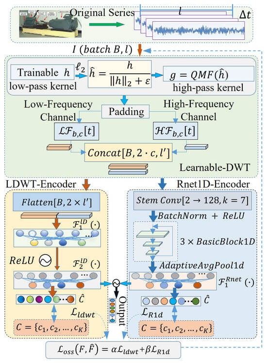
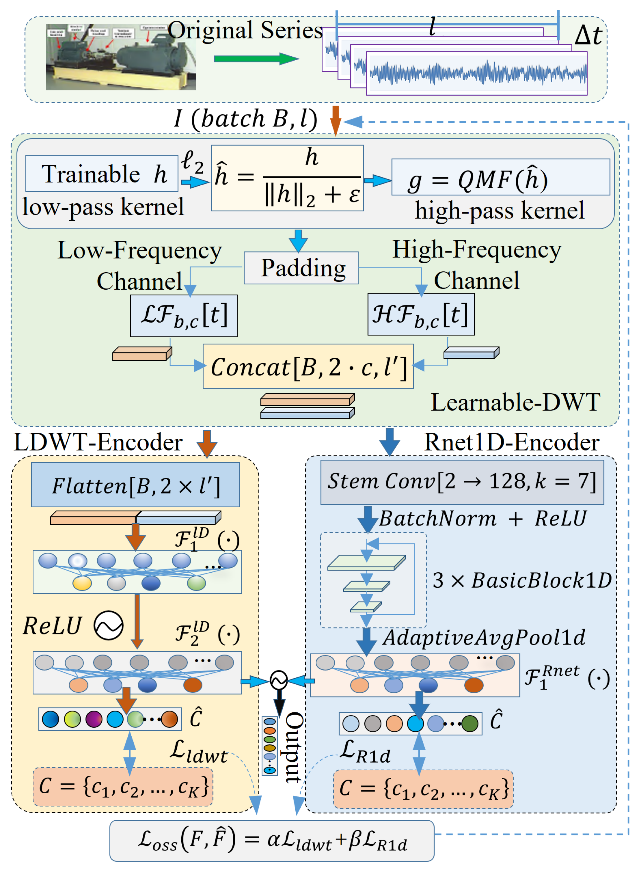
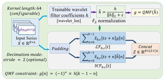
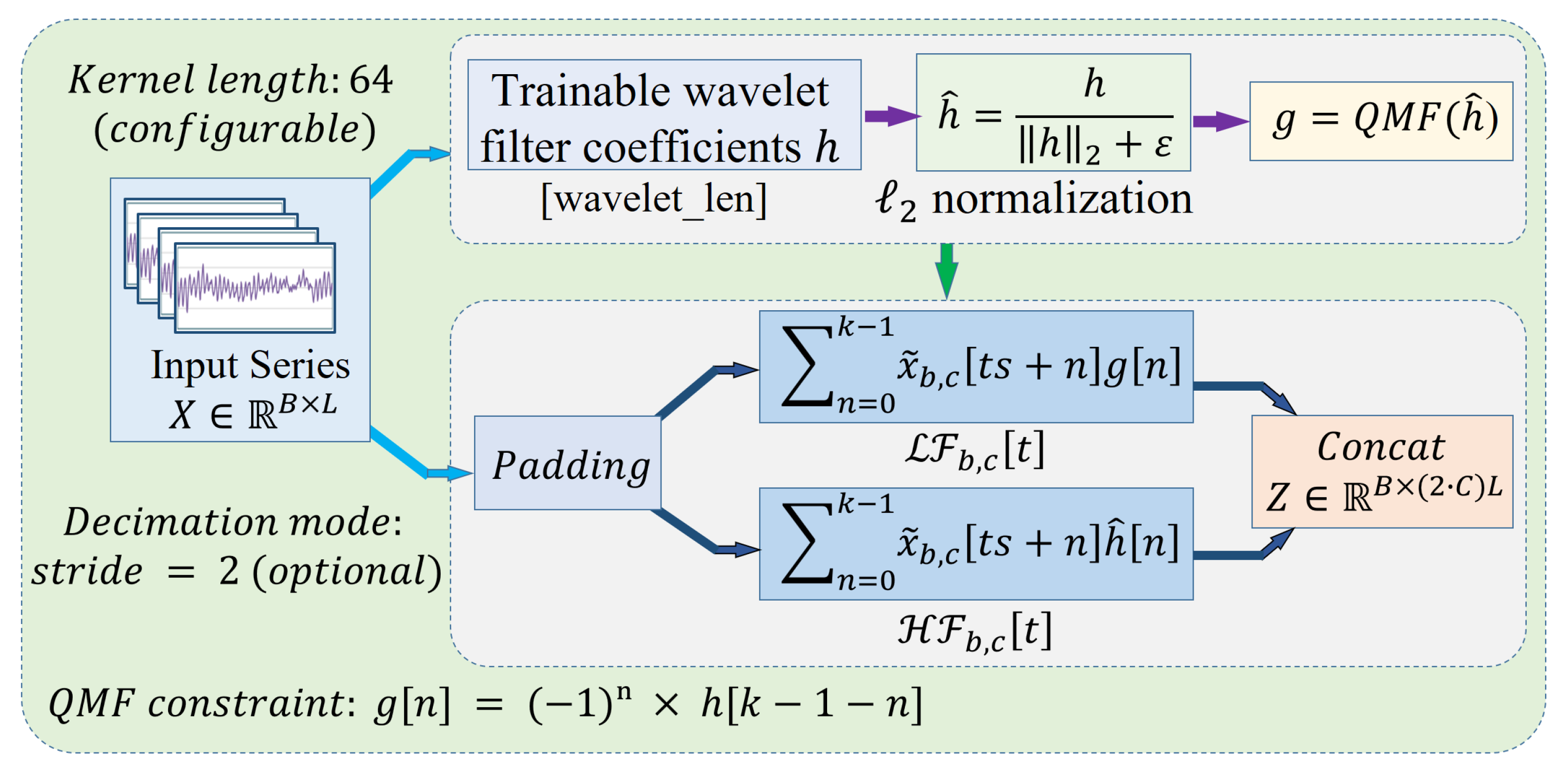
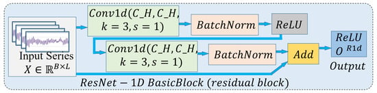
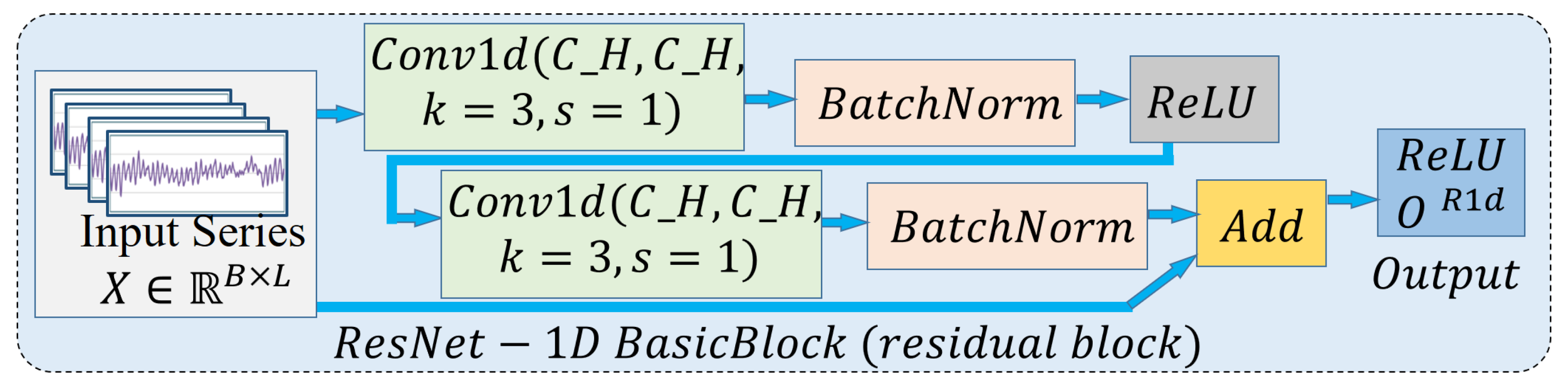
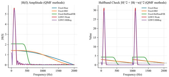
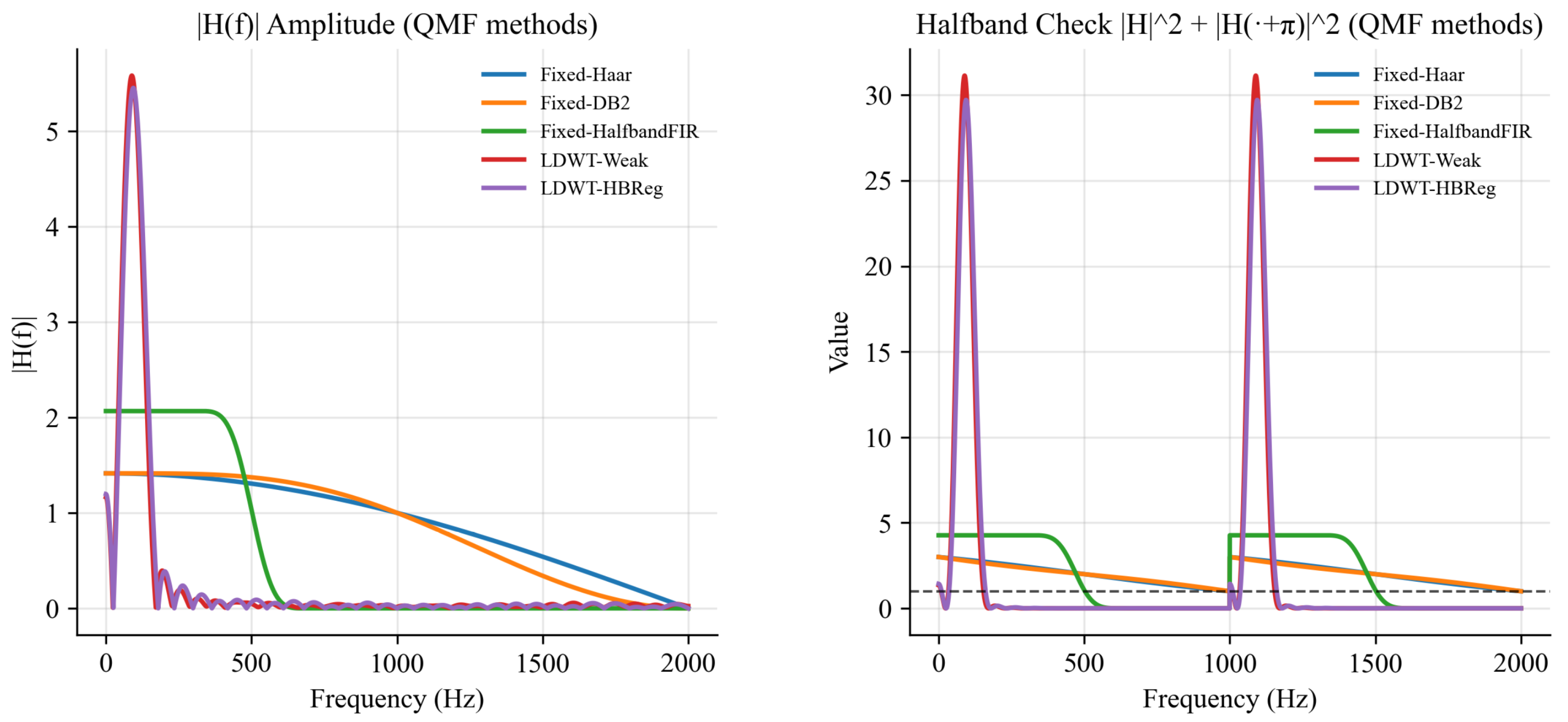
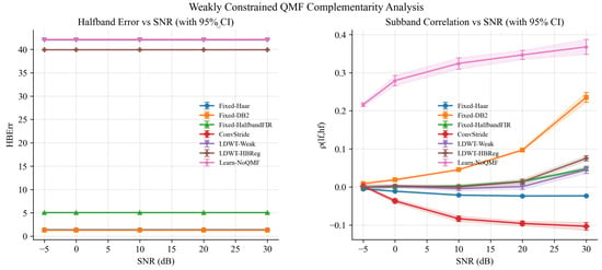
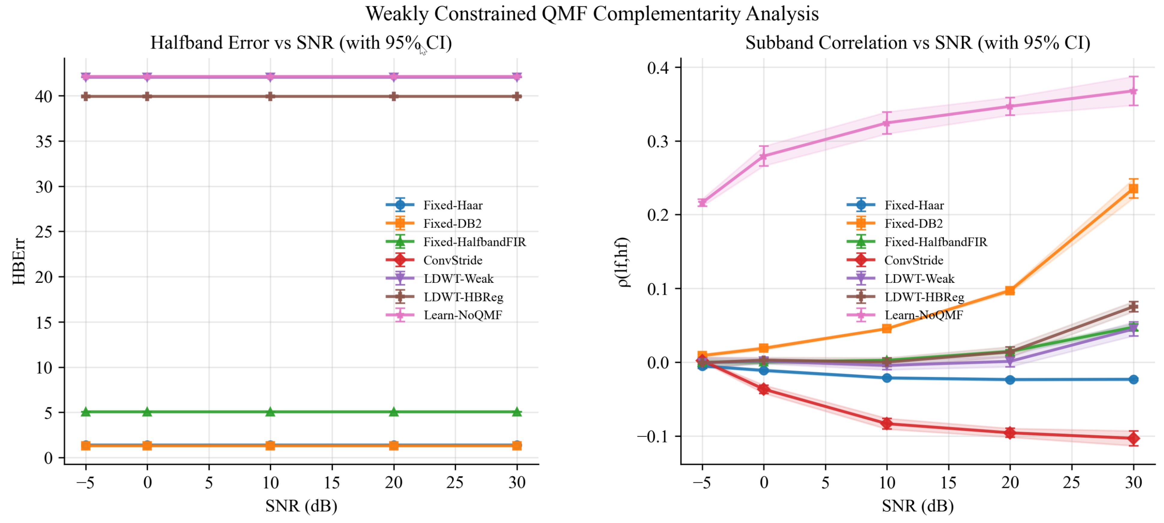
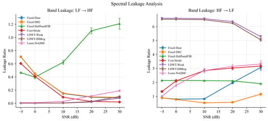
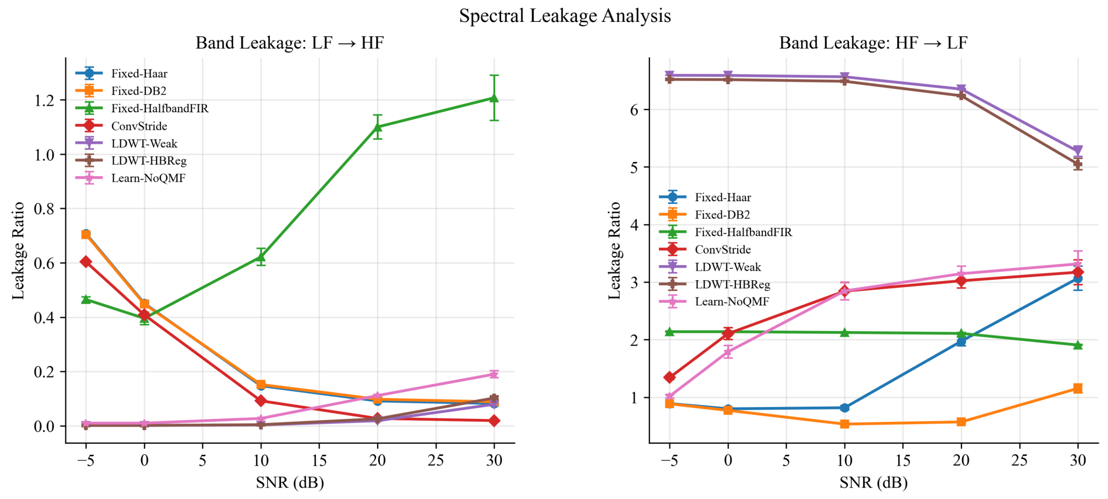
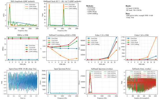
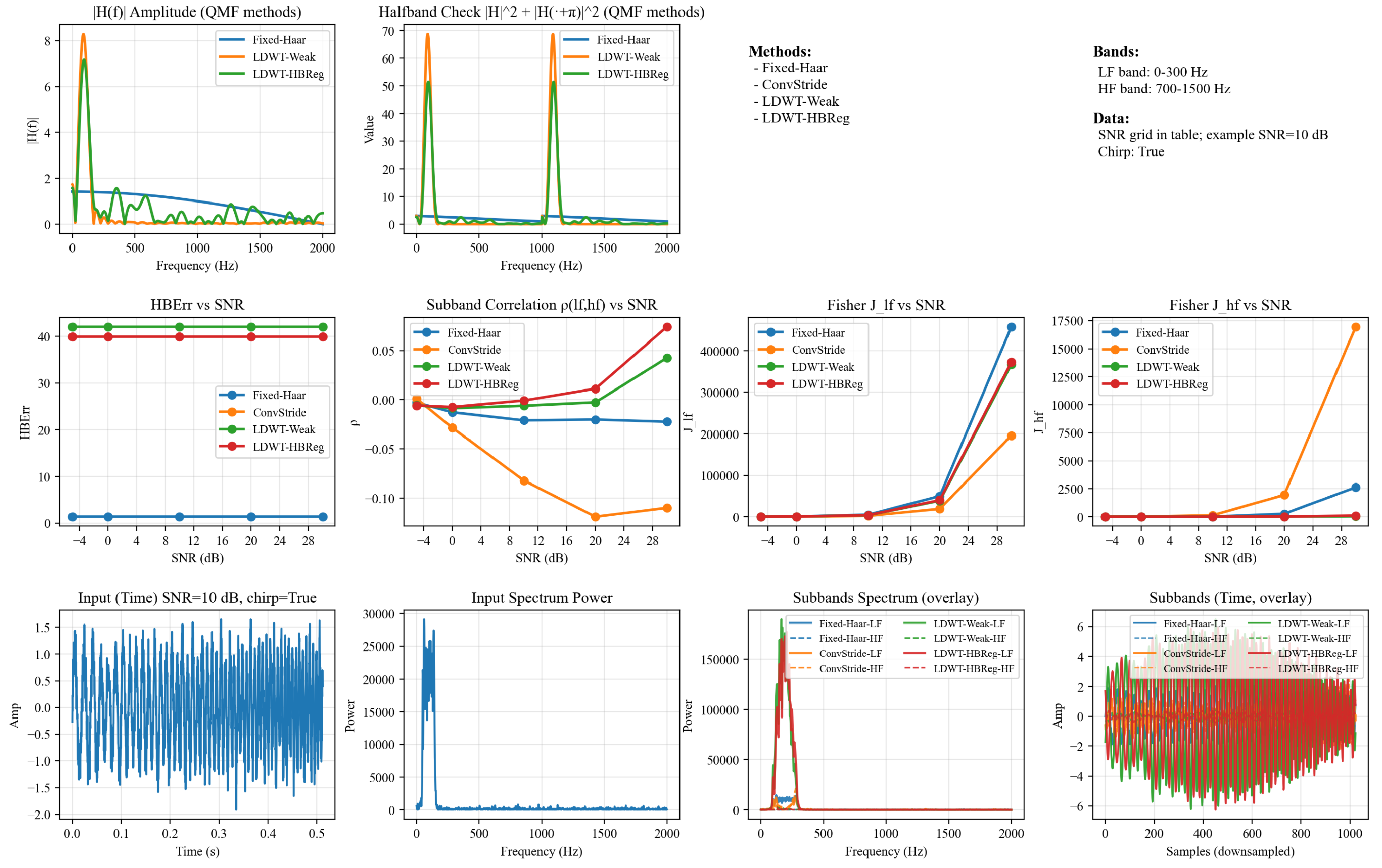
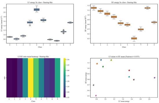
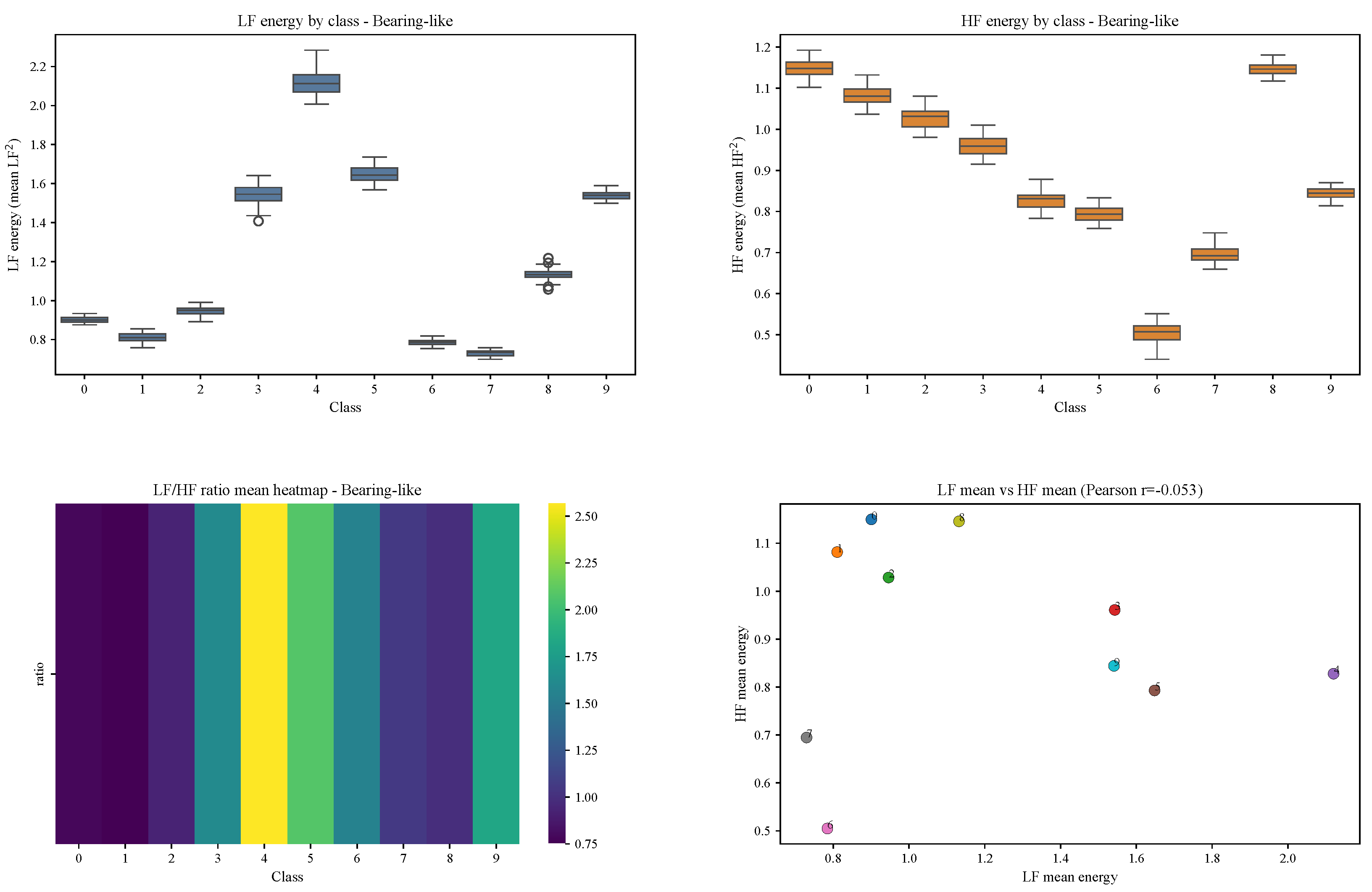
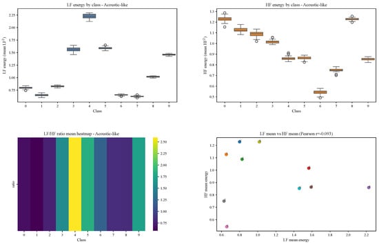
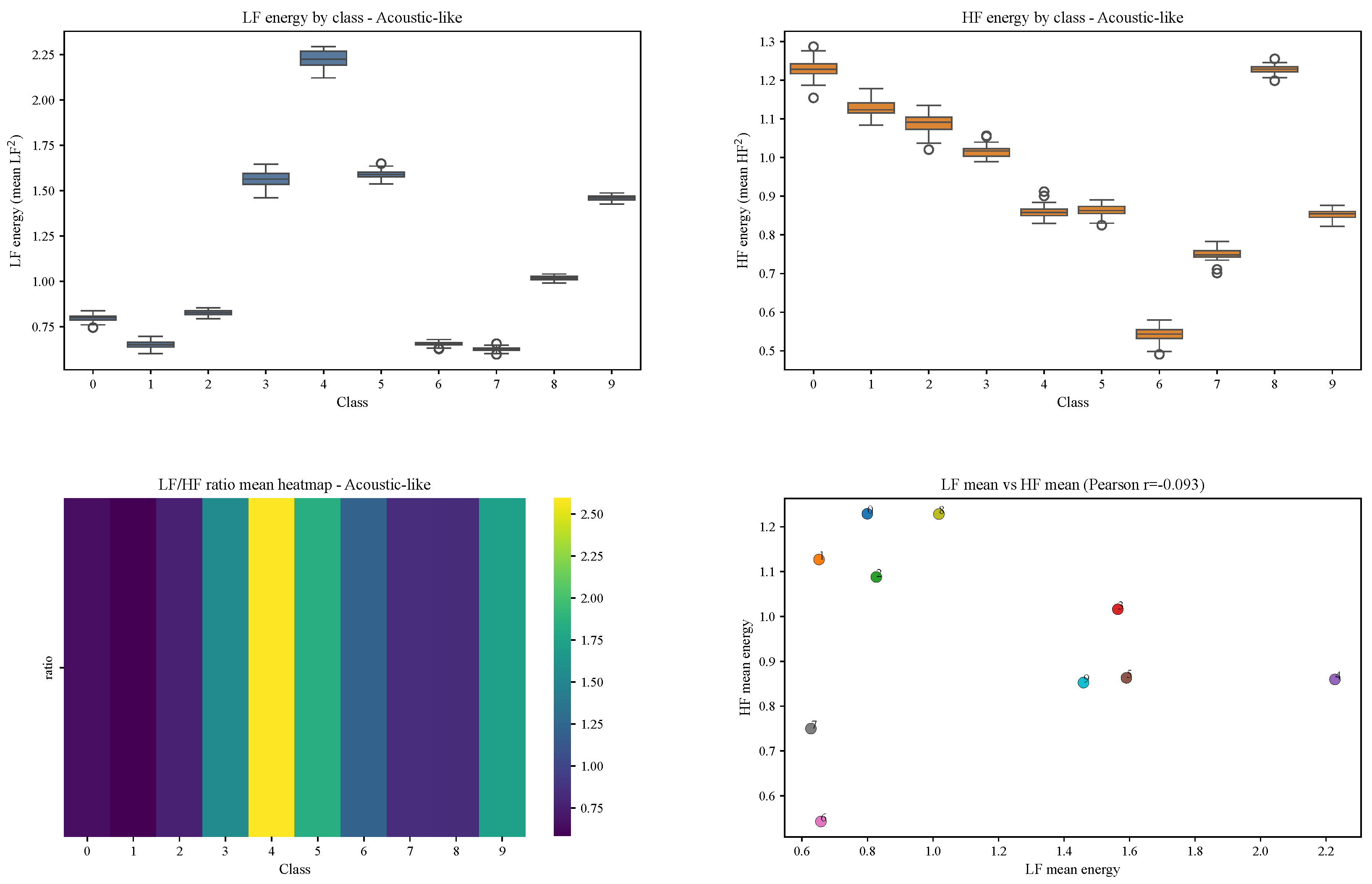
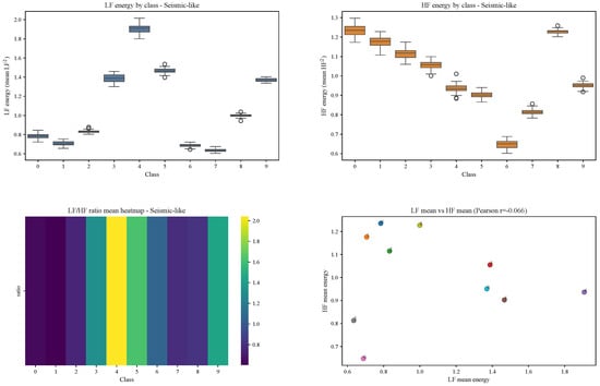
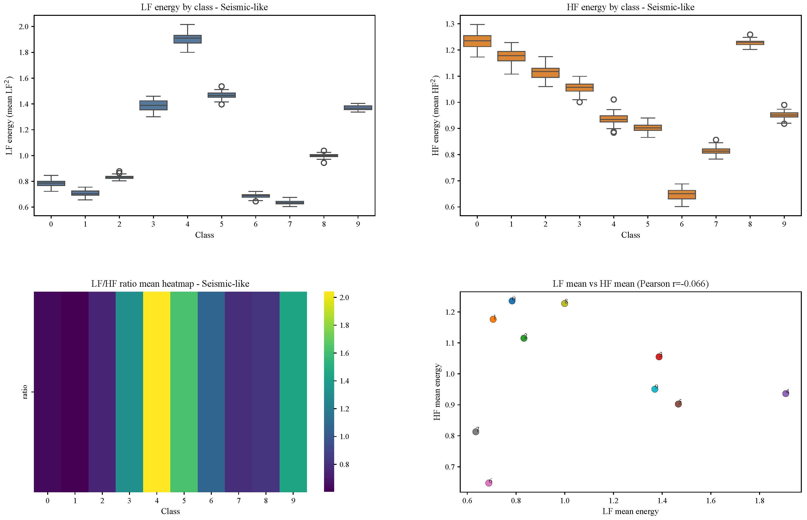
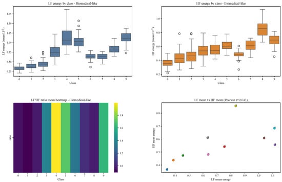
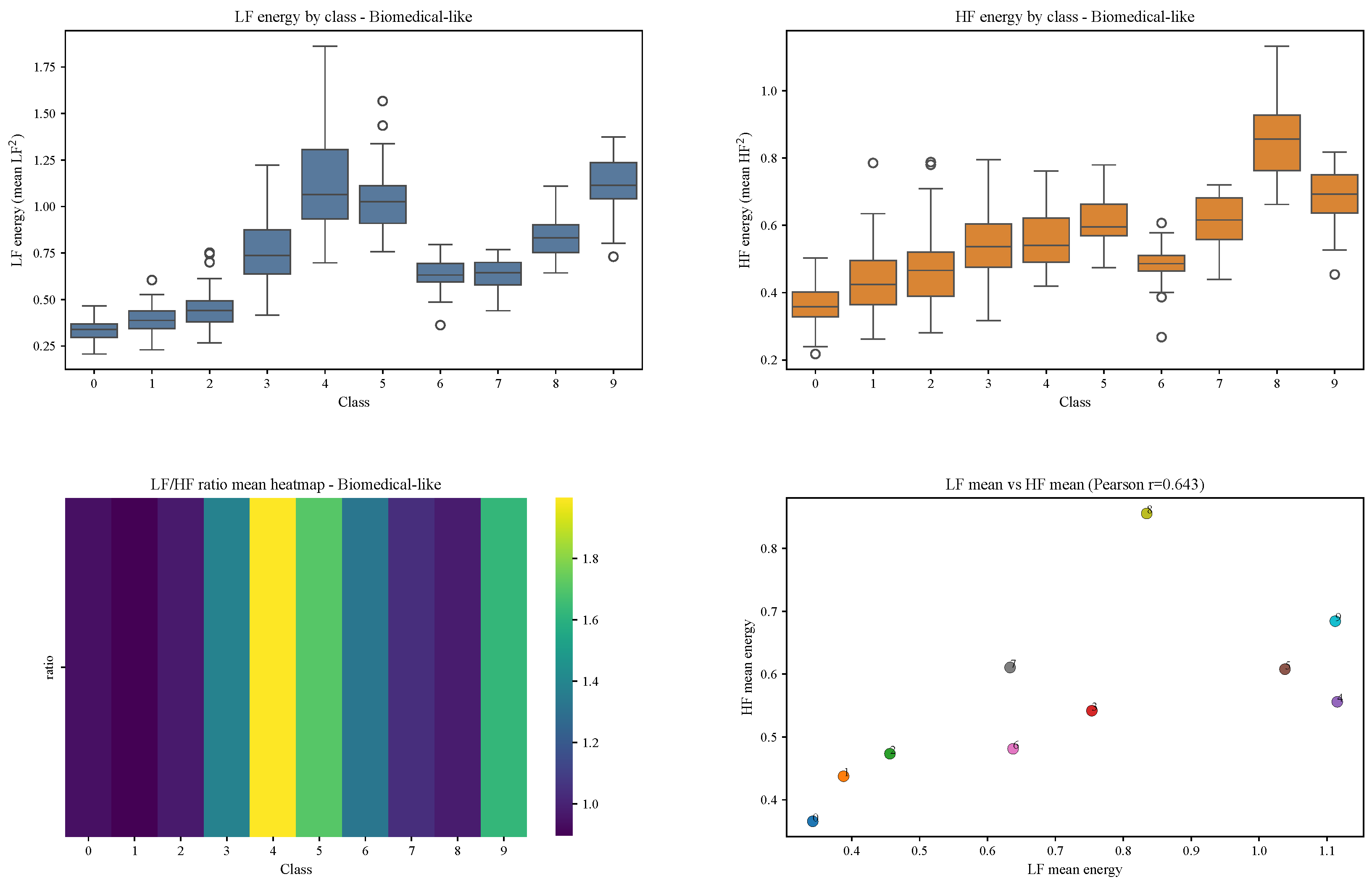
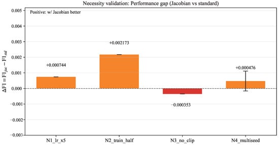
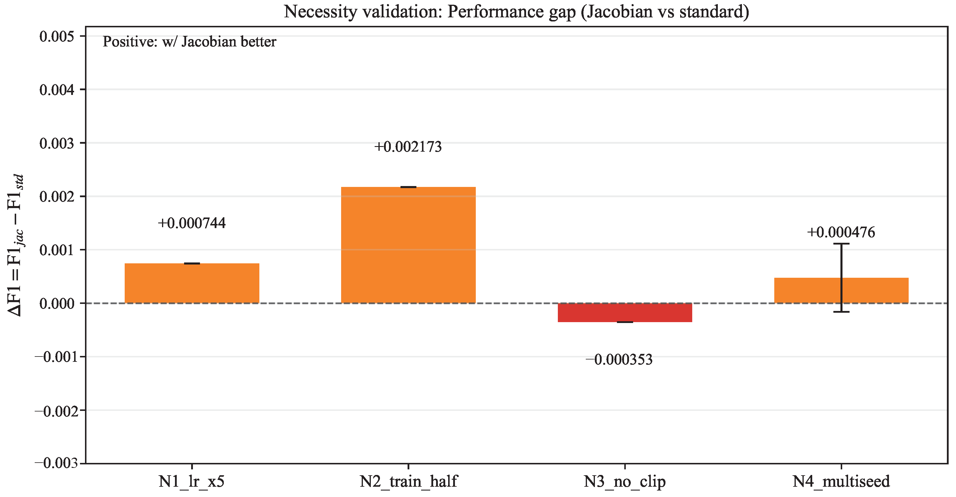
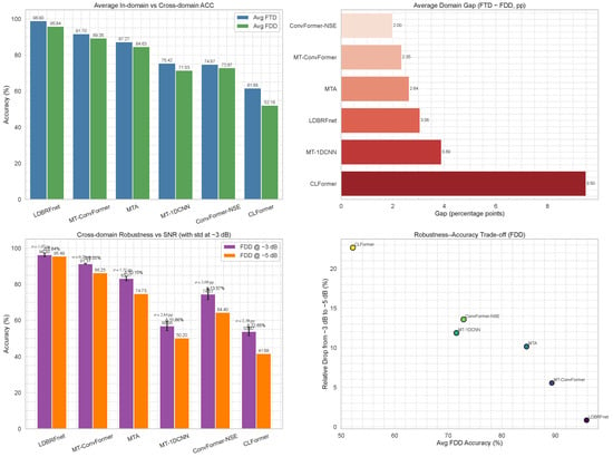
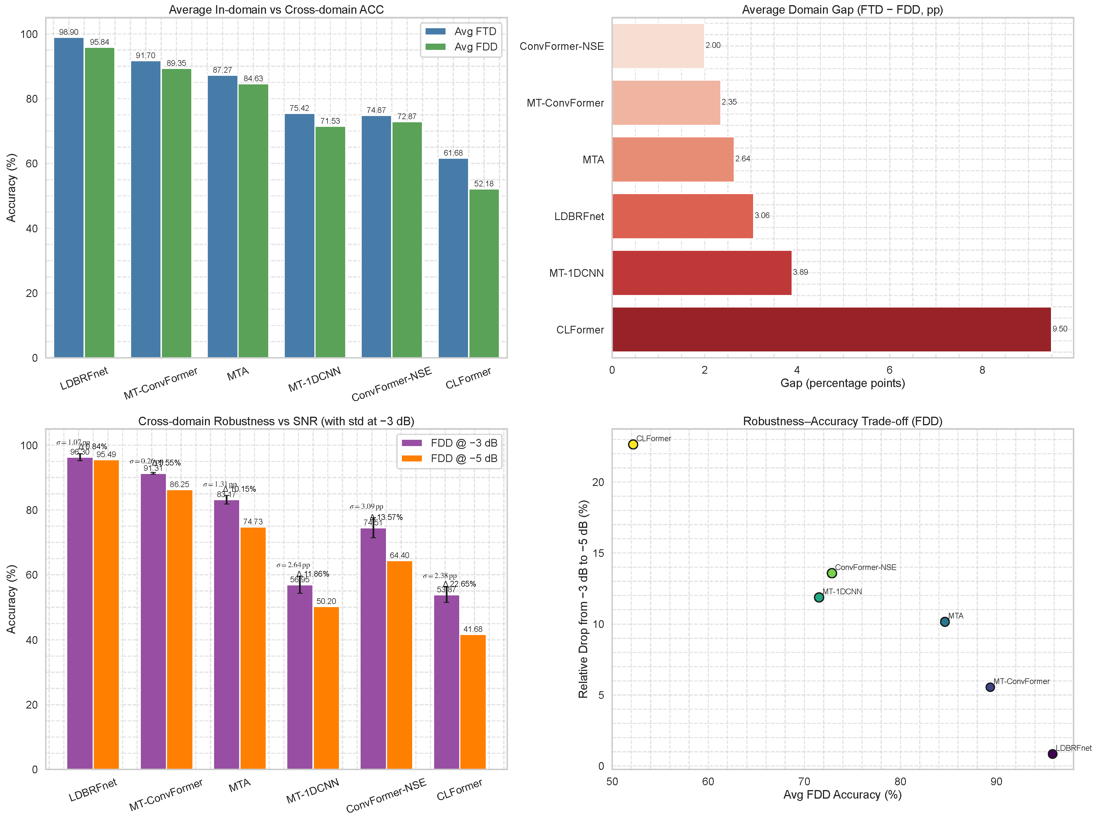
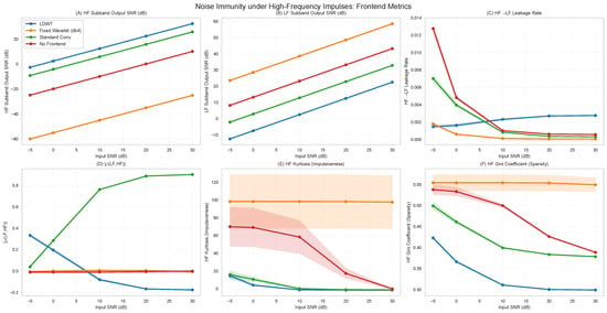
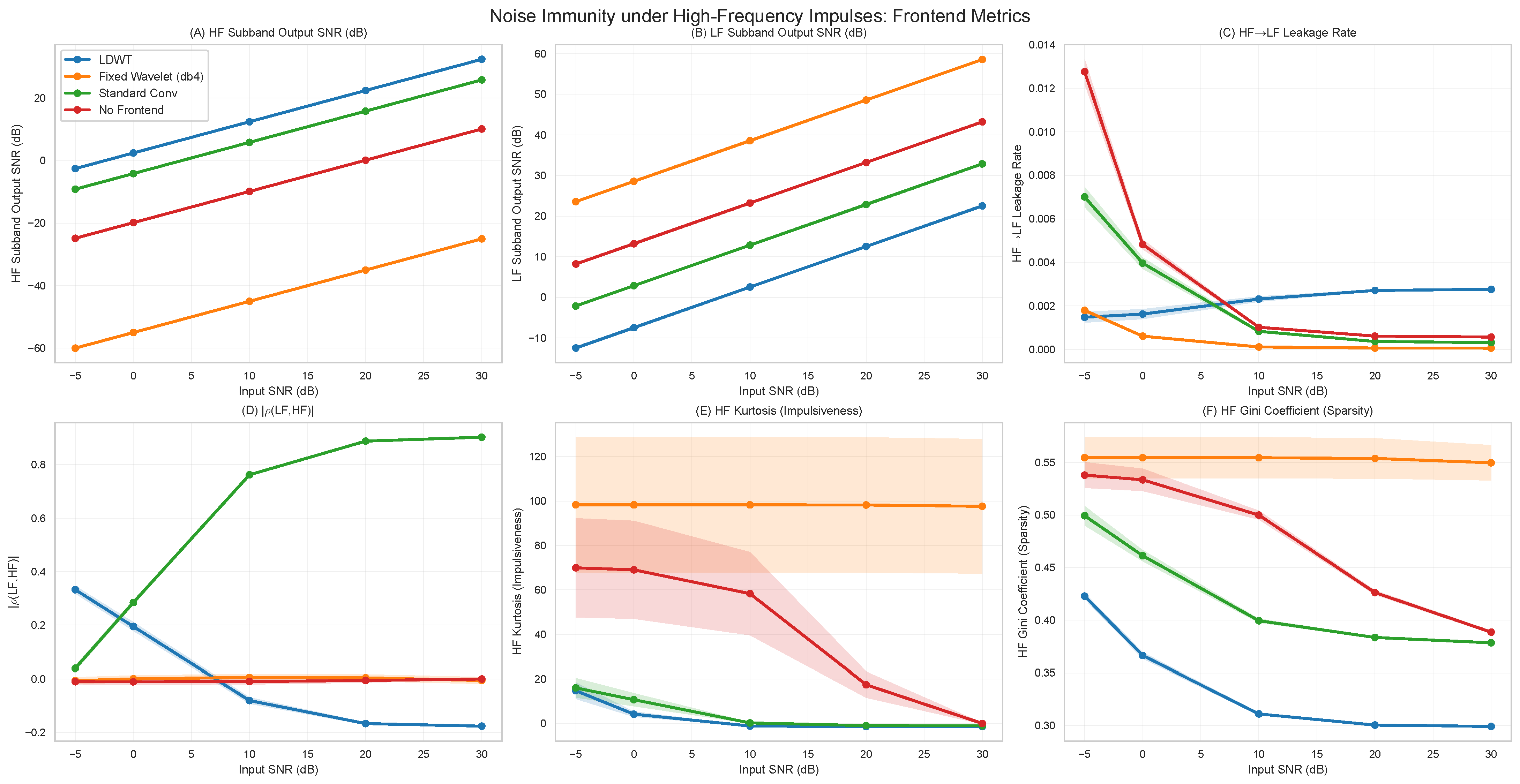

Disclaimer/Publisher’s Note: The statements, opinions and data contained in all publications are solely those of the individual author(s) and contributor(s) and not of MDPI and/or the editor(s). MDPI and/or the editor(s) disclaim responsibility for any injury to people or property resulting from any ideas, methods, instructions or products referred to in the content. |
© 2026 by the authors. Licensee MDPI, Basel, Switzerland. This article is an open access article distributed under the terms and conditions of the Creative Commons Attribution (CC BY) license.