Chance-Constrained Distributed Optimization with Shared States

Abstract

Interconnected systems have attracted significant attention in numerous engineering applications such as energy, water, and oil, as well as gas distribution networks. However, due to their high complexity, it is enormously difficult to ensure a reliable and effective cooperation of such interconnected systems under limited communication and interaction capacities. In addition, uncertainty consideration poses further challenges in developing an efficient distributed optimization approach to such interconnected systems. Furthermore, satisfying the constraints of shared states between subsystems under uncertainty leads to conflict issues and has not been properly studied yet. This study proposes a chance-constrained distributed optimization approach to the optimal operation of interconnected systems by considering conflicting reliability levels of satisfying shared state constraints. A compromised reliability level for such constraints is determined by an averaged weighting. We establish that the optimal cost is Lipschitz-continuous with respect to the compromised reliability level, providing a theoretical basis for quantifying the marginal cost of reliability, and we show that the compromise is robust to perturbations in the subsystem weights. We develop a numerical solution framework based on the inner–outer approximation method. For the efficient computation of the high-dimensional integrals, we use Hoeffding’s inequality to determine a suitable sample size. The optimal operation of three interconnected energy distribution networks is used as a case study to demonstrate the proposed approach.

1. Introduction

Between interconnected systems, there are usually shared (coupled) state variables influenced by the connecting subsystems. The control or management of these shared states is essential for achieving optimal performance, robustness, and resilience, which has not been properly studied until now. Instead, in most previous studies, the coupling of interconnected systems has been considered as a control mechanism for the subsystems to coordinate their operations toward individual and global objectives while maintaining local autonomy and privacy [1,2]. This approach has been applied in many applications, such as autonomous vehicles, robotics, energy systems, water networks, and unmanned aerial vehicles (UAVs) [3,4]. However, in many applications, subsystems share physical states (e.g., locations of connected UAVs and collaborative robots, power flows between energy systems, and water flows between water distribution networks). Therefore, it is necessary to deal with state sharing among interconnected systems [5]. The shared states of subsystems are communicated through communication channels or physical couplings. For instance, for a multi-area power system to maintain a stable power supply, information about local generation levels, voltage and frequency deviation, and storage levels need to be shared. Likewise, for multi-robot systems to avoid collisions and enhance collaborative tasks, position and velocity states have to be shared with each other. Achieving consensus on these shared states is not trivial since each subsystem operates to pursue its own benefits. In addition, the presence of uncertainties across the subsystems makes the shared states uncertain, leading to further challenges to control or manage them.

Uncertainties arise from various sources, including the use of simplified or inaccurate system models, measurement inaccuracy, forecasting errors, environmental disturbances, parameter and various approximations [6]. The fluctuation of demands, as well as market prices, poses uncertainties and complicates supply–demand balances in many industrial applications. The intermittency of renewable energy resources, such as solar intensity and wind speed, impose uncertain power generation [7]. In multi-robot systems or sensor networks, random delays, communication failures, hardware degradation, and environmental uncertainties introduce uncertain system behaviors [8]. Furthermore, interconnecting systems not only introduces additional uncertainties due to communication delays and fluctuating topology but also introduces cascading uncertainty concerns among the interconnected systems [9,10].

Distributed optimization algorithms have evolved to address large-scale problems by decomposing them into smaller subproblems with minimal information sharing. An early classical approach is dual decomposition, but it slows under tight coupling and in nonconvex settings [11]. To address some of these limitations, the Alternating Direction Method of Multipliers (ADMM) was subsequently introduced, guaranteeing a linear convergence for convex optimization problems [12]. Despite the improved performance, ADMM lacks a convergence guarantee for nonconvex problems [13]. To solve nonconvex problem in a distributed manner, the Augmented Lagrangian Based Alternating Direction Inexact Newton (ALADIN) algorithm was proposed [13]. ALADIN combines the augmented Lagrangian framework with inexact Newton and active set methods, resulting into a distributed optimization algorithm with a superlinear convergence. Although ALADIN has been extensively applied to different interconnected systems, very few adaptations are available to address distributed optimization problems under uncertainty. The presence of uncertainties in interconnected systems leads to enormous difficulties for optimizing such systems.

Approaches to optimization problems under uncertainty can be classified based on the available information about the uncertainties and the level of conservativeness to the uncertainties. The two-stage stochastic programming is commonly used in process engineering and operational research, where an initial decision is made before the uncertain parameter realization, followed by a corrective action after the realization [14]. Robust optimization enforces worst-case feasibility and is widely used in safety-critical applications, but it is conservative [15]. Scenario-based approaches, such as Sample Average Approximation (SAA) replace uncertainty with sampled realizations, yet they suffer from the curse of dimensionality, and the solution obtained may not be feasible [16]. Chance-constrained optimization (CCOPT) was proposed and widely used in different engineering applications [6,17,18], with recent applications including the chance-constrained sizing of hybrid PV/battery/hydrogen isolated microgrids [19] and chance-constrained AC security constrained optimal power flow [20]. The idea of CCOPT is to achieve a degree of safety in decisions by allowing a predefined violation threshold for operation constraints, leading to a controlled conservativeness. However, CCOPT is known as a hard, intractable problem due to probabilistic constraints [6]. Generally, CCOPT is a non-smooth optimization problem. Several studies have addressed particular cases of CCOPT problems by employing the properties of the distribution of uncertain parameters, the inequality constraint function, and the probability level [21,22].

Recently, smoothing approaches to chance constraints have been proposed; refer to [6] for more information. It is worth noting that our recently proposed inner–outer approximation approach, instead of solving the intractable CCOPT, solves two amenable smooth nonlinear program (NLP) problems whose respective feasible sets sandwich the feasible set of the CCOPT [23,24,25]. In this study, we extend the inner–outer approximation approach to the optimization of interconnected systems under uncertainty.

Although the orchestration of chance-constrained and distributed optimization is evident across different applications, relatively few studies have integrated both of these frameworks. Distributed optimization has been widely adopted for engineering applications such as economic dispatch, large-scale resource allocation, and multi-agent networks [26,27]. However, when addressing uncertainties in this domain, studies often rely on scenario-based approaches [28], which require large sample sizes, or distributionally robust techniques [29,30,31], which tend to produce overly conservative, worst-case solutions.

In the context of competitive multiobjective optimization, some studies considered stochastic objective functions and deterministic constraint sets, while others only focused on the transformation of a stochastic multiobjective optimization problem into a deterministic one [32,33]. While studying chance-constrained multi-objective optimization, Hu and Cho [34] identified the impact of the reliability level on some of the objective functions. This method introduces a fairness concern in interconnected systems with shared states, particularly when subsystems involve conflicting reliability requirements.

In this study, we propose a chance-constrained distributed optimization (CCDOPT) formulation for interconnected systems with shared states. The states are shared in a pairwise coupling in an undirected graph architecture of the interconnected systems. In addition to the local chance constraints inside the individual subsystems, we consider chance constraints on the shared states to ensure a reliability level for either fault tolerance or holding safety requirements. However, as these states are shared by multiple subsystems, they may demand different reliability levels for the safety of these states. To address such conflicting reliability requirements, we propose a compromising approach using a weighted average method, commonly used in multi-objective optimization, to enhance the fairness among the interconnected systems. In this study, we extend our recent conference contribution [35] that applied the inner–outer approximation approach to the chance-constrained optimization optimal power flow in distributed energy networks.

To the best of our knowledge, no study has specifically investigated chance constraints of shared states, leaving a significant gap in the literature. Unlike coupling chance constraints which couple states from different subsystems, shared state chance constraints ensure the safety of the states shared by multiple subsystems. In the case of coupling chance constraints, some studies assumed a uniform reliability level across the interconnected systems, while others employed risk allocation methods to determine distinct reliability levels for each subsystem [36]. Moreover, the existing studies have not addressed the competitive aspects arising from conflicting reliability requirements across interconnected systems.

The novelty of the present work is, therefore, a combination of distributed optimization and chance-constrained optimization in the specific setting of shared-state chance constraints with subsystem-specific and potentially conflicting reliability requirements. Coupled constraints in distributed systems can be either shared-control constraints, which depend only on control variables and are, therefore, deterministic, or shared-state constraints, which depend on state variables that are themselves functions of control and uncertain variables and are, therefore, stochastic [37,38]. The present study addresses the latter case by using chance constraints. The proposed framework also differs from risk-allocation approaches [36], in which risks are assigned to the subsystem that can best control or absorb them, requiring different known risk-absorbing capacities. In contrast, a shared-state chance constraint fixes the likelihood that the constraint must satisfy, rather than minimize, it, and the satisfaction of this likelihood requires distinct contributions from each subsystem. The case of competing per-subsystem reliability requirements addressed in this work and the corresponding compromise mechanism have not been covered previously by either coupled-constraint or risk-allocation formulations, nor by recent work on coupling chance constraints in stochastic dynamic games [39] that imposes a single shared reliability level across coupled agents.

In this study, we define chance constraints on shared states of interconnected systems and address the issue of the resulting reliability dominance when the subsystems demand different reliability levels. We counter this with a compromised reliability level for each shared state through average weighting. We establish the Lipschitz continuity of the optimal cost with respect to the compromised reliability level, providing a computable marginal cost of reliability, and we prove that the compromise is robust to perturbations in the subsystem weights. Methodologically, we extend the inner–outer smoothing approach to a distributed problem formulation, which is solved with ALADIN. Moreover, we provide a Hoeffding-based sample-size guarantee for the Monte-Carlo evaluation of the high-dimensional integral. Finally, a two-area power system is used to demonstrate the proposed approach.

This paper is organized as follows. In Section 2, we present the general problem formulation of chance-constrained distributed optimization (CCDOPT) for interconnected systems with shared states. In Section 3, the proposed solution approach to the CCDOPT is derived. Numerical implementation is discussed in Section 4, while, in Section 5, we use a case study to demonstrate the efficacy of our approach. Conclusions and future work are presented in Section 6.

2. Problem Definition

An interconnected system consists of multiple subsystems or control areas that operate independently yet are linked physically or via wireless communication or share infrastructure such as storage and demand. We model such a system as an undirected graph in which nodes represent subsystems and edges represent direct interconnections [26].

Definition 1.

Let $\mathcal{G}=(\mathcal{V},\mathcal{E})$ denote an undirected graph representing the interconnected system, where:

• $\mathcal{V}=\{1,2,\dots ,N_s\}$ is the set of nodes, with each corresponding to a subsystem.
• $\mathcal{E}=\left\{\{i,j\}\subseteq \mathcal{V}\mid i\ne j,i\mathrm{is}\mathrm{directly}\mathrm{connected}\mathrm{to}j\right\}$ is the set of edges, representing direct interconnections between subsystems.

For each subsystem, i, let ${\mathcal{N}}_i=\{j\in \mathcal{V}\mid (i,j)\in \mathcal{E}\}$ denote the set of subsystems directly interconnected to i.

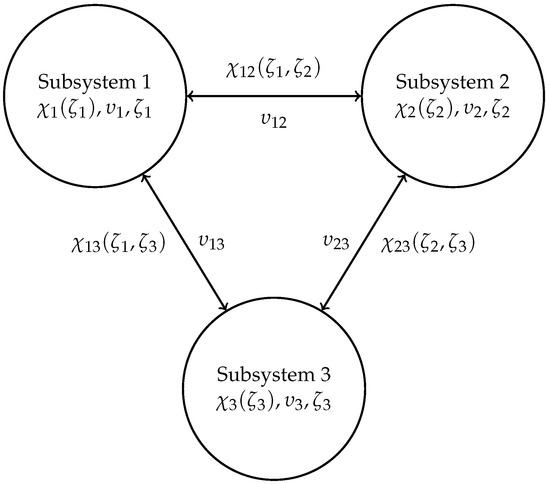
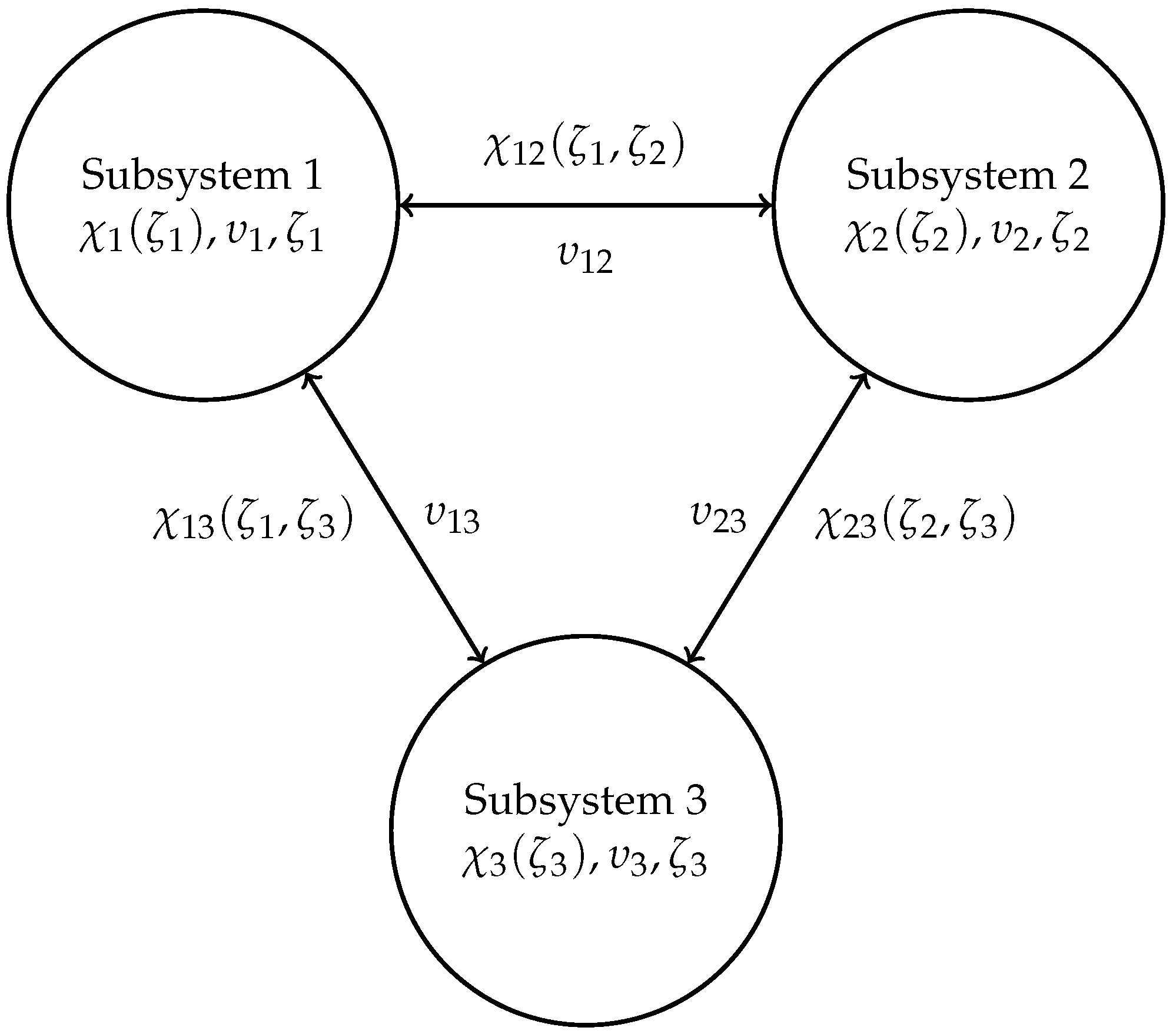
Figure 1 illustrates an interconnected system with $N_s=3$ subsystems. Taking subsystem 1 as a reference, its core (ego) state, control, and random variables are ${\chi }_1\left({\zeta }_1\right)$, ${\upsilon }_1$, and ${\zeta }_1$, respectively. Subsystem 1 is directly connected to both subsystem 2 and subsystem 3; thus, ${\mathcal{N}}_1=\{2,3\}$. The shared state and control variables between subsystem 1 and subsystem $j\in {\mathcal{N}}_1$ are ${\chi }_{1j}({\zeta }_1,{\zeta }_j)$ and ${\upsilon }_{1j}$, carried on edge $(1,j)\in \mathcal{E}$. The core state variables are subject to uncertainties within each subsystem, while the shared state variables are affected by the uncertainties of both connected subsystems. It is noted that, in most previous studies on distributed systems, only shared control variables, ${\upsilon }_{ij}$, have been considered, leading to a relatively simple problem formulation. In addition, instead of coupled state constraints of the form $s({\chi }_i\left({\zeta }_i\right),{\chi }_j\left({\zeta }_j\right))\le 0$, we consider shared state chance constraints of the form $\mathrm{Pr}\{s\left({\chi }_{ij}({\zeta }_i,{\zeta }_j)\right)\le 0\}\ge \alpha$ in this study.

Figure 1. An interconnected system with three subsystems. Each node contains the local state, control, and random variables of the subsystem. Each edge carries the shared state ${\chi }_{ij}({\zeta }_i,{\zeta }_j)$ and shared control ${\upsilon }_{ij}$ between subsystems i and j.

2.1. Problem Statement

We now define a chance-constrained distributed optimization problem for the interconnected system $\mathcal{G}=(\mathcal{V},\mathcal{E})$, where each subsystem $i\in \mathcal{V}$ has its state, control, and random variables:

$$\begin{array}{cc}\hfill \underset{\upsilon }{min}& \sum _{i=1}^{N_s}{w}_i\mathbb{E}\left[f_i\left({\chi }_i\left({\zeta }_i\right),{\chi }_{ij}({\zeta }_i,{\zeta }_j),{\upsilon }_i,{\upsilon }_{ij}\right)\right]\hfill \end{array}$$

(1a)

$$\begin{array}{cc}\hfill \mathrm{s}.\mathrm{t}.& \hfill G_i\left({\chi }_i\left({\zeta }_i\right),{\chi }_{ij}({\zeta }_i,{\zeta }_j),{\upsilon }_i,{\upsilon }_{ij},{\zeta }_i\right)=0,\end{array}$$

(1b)

$$\begin{array}{c}Pr\left\{s_i\left({\chi }_i\left({\zeta }_i\right),{\chi }_{ij}({\zeta }_i,{\zeta }_j),{\upsilon }_i,{\upsilon }_{ij},{\zeta }_i\right)\le 0\right\}\ge {\alpha }_i,\hfill \end{array}$$

(1c)

$$\begin{array}{c}{\upsilon }_i\in {\mathrm{{\rm Y}}}_i,{\upsilon }_{ij}\in {\mathrm{{\rm Y}}}_i\cap {\mathrm{{\rm Y}}}_j,\hfill \end{array}$$

(1d)

$$\begin{array}{c}{w}_i>0.\hfill \end{array}$$

(1e)

Constraints (1b)–(1d) hold for all $i\in \mathcal{V}$, $j\in {\mathcal{N}}_i$, and ${\zeta }_i\in Z_i$. We assume that the uncertainty in any subsystem i, denoted as ${\zeta }_i\in Z_i\subset {\mathbb{R}}^{q_i}$, is a Borel-measurable random variable drawn from a complete probability space $(Z_i,{\mathcal{A}}_i,\mathrm{Pr})$, where $Z_i$ is the sample space, ${\mathcal{A}}_i$ is the $\sigma$-algebra of events, and $\mathrm{Pr}$ is the probability measure with $\mathrm{Pr}\left(Z_i\right)=1$. The random vector ${\zeta }_i\in Z_i\subset {\mathbb{R}}^{q_i}$ represents uncertainties in subsystem i and has a known continuous joint probability density function, ${\varrho }_i\left({\zeta }_i\right)$.

For each subsystem i, state variables are denoted as ${\chi }_i\left({\zeta }_i\right)\in {\mathbb{R}}^{n_i}$, and the control variables are ${\upsilon }_i\in {{\rm Y}}_i\subset {\mathbb{R}}^{p_i}$, where ${\mathrm{{\rm Y}}}_i$ is a compact set representing the feasible control actions. The notation ${\chi }_i\left({\zeta }_i\right)$ indicates the uncertainty propagation through the state variable in subsystem i. The shared state variable between subsystems i and j is denoted as ${\chi }_{ij}({\zeta }_i,{\zeta }_j)\in {\mathbb{R}}^{n_{ij}}$. Similarly, the shared control variable is denoted as ${\upsilon }_{ij}\in {\mathrm{{\rm Y}}}_i\cap {\mathrm{{\rm Y}}}_j\subset {\mathbb{R}}^{p_{ij}}$.

In (1a), the function $f_i:{\mathbb{R}}^{n_i}\times {\mathbb{R}}^{n_{ij}}\times {\mathbb{R}}^{p_i}\times {\mathbb{R}}^{p_{ij}}\to \mathbb{R}$ represents the cost associated with subsystem i. $\mathbb{E}$ is the expectation operator. In practice, the objective function (1a) can be generation costs, operation losses, or deviation from a predefined operating trajectory. The objective functions of individual subsystems can be equally weighted or, alternatively, some subsystems can obtain more preference based on their contribution to the total system. Common approaches to determine the weights are rating and ranking methods, and the prior articulation of preferences, as discussed in [40]. In this study, we assume that the weights $w_i,\forall i\in \{1,\dots ,N_s\}$ are given from prior negotiation among the subsystems.

In the equality constraint (1b), for each subsystem i, the function $G_i:{\mathbb{R}}^{n_i}\times {\mathbb{R}}^{n_{ij}}\times {\mathbb{R}}^{p_i}\times {\mathbb{R}}^{p_{ij}}\times {\mathbb{R}}^{q_i}\to {\mathbb{R}}^{m_i}$ represents the system model. The model equations ensure adherence to the physical laws and balance equations governing the dynamics of the subsystems.

The inequality constraints $s_i\left({\chi }_i\left({\zeta }_i\right),{\chi }_{ij}({\zeta }_i,{\zeta }_j),{\upsilon }_i,{\upsilon }_{ij},{\zeta }_i\right)\le 0$, where $s_i:{\mathbb{R}}^{n_i}\times {\mathbb{R}}^{n_{ij}}\times {\mathbb{R}}^{p_i}\times {\mathbb{R}}^{p_{ij}}\times {\mathbb{R}}^{q_i}\to {\mathbb{R}}^{k_i}$ represent operational or capacity restrictions of subsystem i, such as the storage capacity and sharing area limit. The aim of chance constraints in Equation (1c) is to ensure that the inequality constraints be held above a user-defined probability level, ${\alpha }_i\in (0.5,1)$, reflecting the desired reliability of subsystem i. Difficulties arise from the chance constraints of shared states between subsystems (1c), since the reliability level ${\alpha }_i$ is usually defined by the operator of subsystem i without considering the opinion of the connected subsystems. Although we need only one value for the problem definition, the situation in which individual subsystems demand different confidence levels can arise.

2.2. Compromising Shared State Chance Constraints

To discuss the shared state chance constraints (1c), let us consider the following simplified form:

$$Pr\{{\chi }_{i{j}_{min}}\le {\chi }_{ij}({\zeta }_i,{\zeta }_j)\le {\chi }_{i{j}_{max}}\}\ge {\alpha }_i.$$

(2)

This constraint holds for all $i\in \mathcal{V}$, all j with $(i,j)\in \mathcal{E}$, and all ${\zeta }_i\in Z_i$. The aim of (2) is to keep the share state ${\chi }_{ij}({\zeta }_i,{\zeta }_j)$ in a safety region by a reliability level, ${\alpha }_i$, which is independently defined by each of the interconnecting subsystems. Note that, in our graph formulation, each shared state is associated with an edge, $(i,j)\in \mathcal{E}$, and is, therefore, pairwise.

Taking energy supply for instance, power plants supply energy to hospitals, security and data centers, and financial institutions, etc. The shared state is the power flow from the power plants to the consumers and is to be chance-constrained by the cable capacity. A lower reliability level might be chosen by the power plants to maximize the renewable energy integration and, hence, their profit. On the other side, the energy consumers tend to set the confidence level high to ensure a reliable power supply. Moreover, considering interconnected power systems sharing a battery, keeping the state of charge of the battery above a certain threshold is common in renewable energy integration used during peak hours [41]. Different interconnected power systems may consider different reliability levels to hold the state of charge within the safe range. Therefore, the definition of the value of ${\alpha }_i$ by each individual subsystem leads to conflicts.

A shared state chance constraint introduces a challenge of reliability dominance. Given a shared state chance constraint (2), a subsystem demanding a higher reliability level dominates the others; i.e., holding the constraint for this subsystem is more important than for the other ones. For each edge $(i,j)\in \mathcal{E}$ in the graph $\mathcal{G}$, given that ${\alpha }_i>{\alpha }_j$, the subsystem i dictates the tightest constraint on (2). This forces all interconnected subsystems to be conservative on the shared state, irrespective of their desired constraint violation. This contradicts the fairness of coordination and necessitates a compromising approach for each subsystem to decide on the reliability level of the shared state chance constraint.

To address this issue, we propose a weighted average approach for the problem (1) to decide a commonly acceptable reliability level. The weight of each subsystem on the compromised reliability level can be chosen based on its contribution in the interconnection or from a prior negotiation. Thus, a compromised reliability level for the shared state chance constraint (2) is defined as follows:

$${\alpha }_{ij}={\gamma }_{ij}{\alpha }_i+(1-{\gamma }_{ij}){\alpha }_j,\mathrm{for}\mathrm{all}(i,j)\in \mathcal{E},\mathrm{with}{\gamma }_{ij}\in (0,1).$$

(3)

Specifically, for each shared edge, $(i,j)\in \mathcal{E}$, we assign a single compromise weight, ${\gamma }_{ij}\in (0,1)$, determined from sensitivity (risk impact), responsibility (e.g., average normalized contribution to the shared state), or the negotiated priority between the two subsystems. By construction, ${\alpha }_{ij}$ is a convex combination of ${\alpha }_i$ and ${\alpha }_j$ on the edge $(i,j)\in \mathcal{E}$, so

$$min\{{\alpha }_i,{\alpha }_j\}\le {\alpha }_{ij}\le max\{{\alpha }_i,{\alpha }_j\}.$$

(4)

The practical rationale for the weighted-average compromise is that the reliability level of a shared chance constraint should be determined fairly for each individual subsystem using a compromised value. As a motivating example, consider a shared state representing power flow from generation to consumption, chance-constrained by the cable capacity: the generation side may prefer a lower reliability level to maximize renewable integration and profit, while the consumption side prefers a higher reliability level to ensure supply security. These competing interests need to be reconciled, for instance through negotiation, and the weighted-average rule provides a principled compromise. When there is no such interest conflict, alternative aggregation rules become more appropriate: the maximum reliability for high-safety settings, or the minimum reliability for high-profit settings. The theoretical justification of this choice is provided by Theorem 1 below.

Remark 1.

The compromise weights ${\gamma }_{ij}$ introduced in (3) are associated with a specific shared edge, $(i,j)\in \mathcal{E}$, and should not be confused with the objective-function weights, $w_i$, in (1a), which are defined globally, one per subsystem. A subsystem with multiple neighbors, therefore, carries a single global weight, $w_i$, on its full expected cost but a separate compromise weight, ${\gamma }_{ij}$, on each of its incident shared edges.

It is noted that extensions to hypergraph structures where a state is shared among three or more subsystems would require the generalization ${\alpha }_{\mathcal{H}}={\sum }_{k\in \mathcal{H}}{\gamma }_{\mathcal{H},k}{\alpha }_k$, with ${\gamma }_{\mathcal{H},k}>0$ and ${\sum }_{k\in \mathcal{H}}{\gamma }_{\mathcal{H},k}=1$, over all subsystems k in a hyperedge $\mathcal{H}$. This extension is beyond the scope of the present work.

To enhance reliability-based fairness, in addition to introducing the compromised reliability level ${\alpha }_{ij}$, we adjust the weights in the objective function (1a) by considering the reliability levels of chance constraints demanded by the interconnected subsystems into factors. These factors predetermine the objective weights by a weighted summation, which is commonly used in multi-objective optimization. More specifically, by demanding higher reliability, the subsystem will be penalized in the objective function. The details of this proposed method are presented in the following subsections.

2.3. Assumptions

For further analysis, the following assumptions are considered:

(A1)

For each subsystem, i, the functions $f_i$, $G_i$, and $s_i$ are at least twice differentiable.

(A2)

The interconnection graph $\mathcal{G}$ is fully connected.

(A3)

The interconnected subsystems are of a similar size, and hence, the magnitude of the objective functions $f_i$ for all subsystems $i\in \mathcal{V}$ are of the same range.

The assumption (A1) is realistic in many engineering applications, such as energy, water, and robotics systems, since nonlinear balance equations are generally nonconvex but continuously differentiable. Assuming a full connection in the graph $\mathcal{G}$ in (A2) ensures that there is a communication path between any two subsystems, which is essential for distributed optimization. Assumption (A3) ensures that none of the objective functions of a subsystem is prioritized based on its magnitude, making sense for the associated weights. In the case of different magnitudes, normalization is commonly used, for which various approaches are discussed [40].

2.4. Reliability-Based Fairness by a Weighted Objective Function

To enable the subsystems to jointly solve the optimization problem (1) while sharing only limited information, we define auxiliary (compact) variable vectors ${\eta }_i, {\mathrm{v}}_i$ and $y_i$, representing the random variables influencing subsystem i, its shared control and state variables with the coupling subsystems, respectively [37]:

$$\begin{array}{c}\hfill {\eta }_i={\left[{\zeta }_j\right]}_{\forall j\in {\mathcal{N}}_i}^T,{\mathrm{v}}_i={\left[{\upsilon }_{ij}\right]}_{\forall j\in {\mathcal{N}}_i}^T,y_i\left({\eta }_i\right)={\left[{\chi }_{ij}({\zeta }_i,{\zeta }_j)\right]}_{\forall j\in {\mathcal{N}}_i}^T,\forall i\in \mathcal{V}.\end{array}$$

(5)

where ${\eta }_i$ collects the random variables associated with all neighbors of subsystem i, ${\upsilon }_i$ collects the shared control variables, and $y_i\left({\eta }_i\right)$ stacks the coupling state components associated with those neighbors. Thus, for each $j\in {\mathcal{N}}_i$, the term ${\chi }_{ij}({\zeta }_i,{\zeta }_j)$ represents the part of the state of subsystem i that depends jointly on its own variable ${\zeta }_i$ and the neighboring variable ${\zeta }_j$.

After aggregating the core and auxiliary variables for subsystem i, we have the vectors of unified local variables for each subsystem:

$$\begin{array}{c}\hfill {\xi }_i={[{\zeta }_i,{\eta }_i]}^T,u_i={[{\upsilon }_i,{\mathrm{v}}_i]}^T,x_i\left({\xi }_i\right)={[{\chi }_i\left({\zeta }_i\right),y_i\left({\eta }_i\right)]}^T,\forall i\in \mathcal{V}\end{array}$$

(6)

where ${\xi }_i$ contains all random variables influencing subsystem i, $u_i$ contains both the local shared control variables, and $x_i\left({\xi }_i\right)$ contains both the local and the states shared with the coupled subsystems. In this way, each subsystem can express its local optimization problem entirely in terms of the unified vectors $x_i\left({\xi }_i\right)\in {\mathbb{R}}^{{\mathbf{n}}_i}$, $u_i\in {\mathcal{U}}_i\subset {\mathbb{R}}^{{\mathbf{p}}_i}$ and ${\xi }_i\in {\mathsf{\Omega }}_i\subset {\mathbb{R}}^{{\mathbf{q}}_i}$. Their respective dimensions for subsystem i is as follows:

$$\begin{array}{c}\hfill {\mathbf{q}}_i=q_i+\sum _{j\in {\mathcal{N}}_i}{q}_{ij},{\mathbf{p}}_i=p_i+\sum _{j\in {\mathcal{N}}_i}{p}_{ij},{\mathbf{n}}_i=n_i+\sum _{j\in {\mathcal{N}}_i}{n}_{ij},\forall i\in \mathcal{V}.\end{array}$$

(7)

By defining unified variables (5) and (6), the optimization problem (1) becomes separable across the subsystems since each subsystem depends only on its own local variables. Since the aggregated vectors $x_i\left({\xi }_i\right)$ and $u_i$ each contain both local and shared parts, the coupling constraints act only on the shared parts $y_i\left({\eta }_i\right)$ and ${\mathrm{v}}_i$—there is no direct coupling relation between the local variables of different subsystems. Specifically, $B_i\in {\mathbb{R}}^{r\times {\mathbf{n}}_i}$ and $C_i\in {\mathbb{R}}^{s\times {\mathbf{p}}_i}$ are the matrices describing the connections between the subsystems in the following form

$$B_i=\left[\begin{array}{cc}0& I_{n_{ij}}\end{array}\right],C_i=\left[\begin{array}{cc}0& I_{p_{ij}}\end{array}\right],$$

(8)

where the zero block corresponds to the local part and the identity block selects the shared part of the respective aggregated vectors. The coupling structure enforces the shared variables across subsystems as follows:

$$\sum _{i=1}^{N_s}{B}_i{x}_i\left({\xi }_i\right)=0\mathrm{and}\sum _{i=1}^{N_s}{C}_i{u}_i=0.$$

(9)

Combining (9) into a single constraint:

$$\sum _{i=1}^{N_s}{A}_i\left[\begin{array}{c}{x}_i\left({\xi }_i\right)\\ u_i\end{array}\right]=0,\mathrm{with}{A}_i=\left[\begin{array}{cc}{B}_i& 0\\ 0& C_i\end{array}\right].$$

(10)

Now the optimization problem (1) has a semi-separable structure, with decoupled equations and chance constraints, only coupled with an affine constraint, as follows:

$$\begin{array}{cc}\hfill \underset{\mathbf{u}}{min}& \sum _{i=1}^{N_s}{w}_i\left({\alpha }_i\right)\mathbb{E}\left[f_i\left(x_i\left({\xi }_i\right),u_i\right)\right]\hfill \end{array}$$

(11a)

$$\begin{array}{cc}\hfill \mathrm{s}.\mathrm{t}.& G_i\left(x_i\left({\xi }_i\right),u_i,{\xi }_i\right)=0,\forall i\in \mathcal{V},\hfill \end{array}$$

(11b)

$$\begin{array}{c}Pr\left\{s_i\left(x_i\left({\xi }_i\right),u_i,{\xi }_i\right)\le 0\right\}\ge {\alpha }_{ij},\forall i\in \mathcal{V},j\in {\mathcal{N}}_i,\hfill \end{array}$$

(11c)

$$\begin{array}{c}{\displaystyle \sum _{i=1}^{N_s}}{A}_i\left[\begin{array}{c}{x}_i\left({\xi }_i\right)\\ u_i\end{array}\right]=0,\hfill \end{array}$$

(11d)

$$\begin{array}{c}{u}_i\in {\mathcal{U}}_i,\forall i\in \mathcal{V},\hfill \end{array}$$

(11e)

where each ${\mathcal{U}}_i\subset {\mathbb{R}}^{p_i}$ is compact, and the weights $w_i\left({\alpha }_i\right)>0$ are normalized for the optimization as described in Remark 2 below. The following result shows that the weights $w_i\left({\alpha }_i\right)$ can be determined to obtain a fairness compensation, which is monotonic to their demanded reliability level, ${\alpha }_i$. This does not require the convexity of (11); it relies solely on the convexity of the design profile $\varphi$ in (A4) below.

We first state the assumption of standardization. Let $I:=(0,1)$ and, for each subsystem i, define the following individual parameterized CCOPT problem:

$$\begin{array}{cc}\hfill J_i\left(\alpha \right)& =\underset{u_i}{min}\mathbb{E}\left[f_i(x_i\left({\xi }_i\right),u_i)\right]\hfill \\ \hfill & \mathrm{s}.\mathrm{t}.Pr\{s_i(x_i\left({\xi }_i\right),u_i,{\xi }_i)\le 0\}\ge \alpha ,\alpha \in I.\hfill \end{array}$$

(12)

Assume $J_i\left(\alpha \right)<\infty$ for all $\alpha \in I$.

(A4)

Standardization of weighted value functions. There exist positive functions, $w_i:I\to (0,\infty )$, $i=1,\dots ,N_s$, and a convex function, $\varphi :I\to {\mathbb{R}}_{+}$, such that, for every i and all $\alpha \in I$,

$$w_i\left(\alpha \right)J_i\left(\alpha \right)=\varphi \left(\alpha \right).$$

(13)

Remark 2.

Since the weights are free design parameters, (A4) is constructive: for any chosen convex ϕ, setting $w_i\left(\alpha \right)=\varphi \left(\alpha \right)/J_i\left(\alpha \right)$ is well defined and positive whenever $J_i\left(\alpha \right)>0$. Note that (A4) does not impose ${\sum }_i{w}_i=1$. The normalization needed in (11) is obtained by

$${\overline{w}}_i\left({\alpha }_i\right)={\displaystyle \frac{w_i\left({\alpha }_i\right)}{{\displaystyle \sum _{j=1}^{N_s}{w}_j\left({\alpha }_j\right)}}},$$

(14)

which satisfies ${\overline{w}}_i>0$ and ${\sum }_i{\overline{w}}_i=1$.

Theorem 1

(Monotonic Fairness Compensation). Define

$$F\left(\mathit{\alpha }\right)=\sum _{i=1}^{N_s}{w}_i\left({\alpha }_i\right)J_i\left({\alpha }_i\right),\mathit{\alpha }=({\alpha }_1,\dots ,{\alpha }_{N_s})\in I^{N_s}.$$

(15)

If (A4) holds, then $F\left(\mathit{\alpha }\right)={\sum }_{i=1}^{N_s}\varphi \left({\alpha }_i\right)$ is Schur-convex in α. Consequently, among all profiles with the mean $\overline{\alpha }={\displaystyle \frac{1}{N_s}}{\sum }_{i=1}^{N_s}{\alpha }_i$, the equal-valued profile $(\overline{\alpha },\dots ,\overline{\alpha })$ minimizes F (uniquely when ϕ is strictly convex). By Remark 2, the same holds for the normalized objective ${\sum }_i{\overline{w}}_i\left({\alpha }_i\right)J_i\left({\alpha }_i\right)$.

Proof. 

Under (A4), $F\left(\mathit{\alpha }\right)={\sum }_i\varphi \left({\alpha }_i\right)$ is symmetric and separable with convex summand $\varphi$. Let $g_i\in \partial \varphi \left({\alpha }_i\right)$ and $g_j\in \partial \varphi \left({\alpha }_j\right)$ be subgradients. The monotonicity of the subgradient mapping of a convex function yields

$$({\alpha }_i-{\alpha }_j)(g_i-g_j)\ge 0\mathrm{for}\mathrm{all}i\ne j,$$

(16)

which is the standard subgradient criterion for the Schur-convexity. Hence, F is Schur-convex (see, e.g., [42]). The Schur-convexity implies that, for a fixed mean, any mean-preserving spread cannot reduce F (Karamata’s inequality), i.e., the minimum occurs at $(\overline{\alpha },\dots ,\overline{\alpha })$. The strict convexity of $\varphi$ gives the uniqueness of the solution.    □

Corollary 1

(Approximate standardization). Assume that there exists a convex $\varphi :I\to {\mathbb{R}}_{+}$ and $\vartheta \ge 0$, such that

$$\underset{i=1,\dots ,N_s}{sup}\underset{\alpha \in I}{sup}|w_i\left(\alpha \right)J_i\left(\alpha \right)-\varphi \left(\alpha \right)|\le \vartheta .$$

(17)

Then, for any $\mathit{\alpha }\in I^{N_s}$ with mean $\overline{\alpha }$:

(a) 

Sandwich:    $|F\left(\mathit{\alpha }\right)-{\sum }_{i=1}^{N_s}\varphi \left({\alpha }_i\right)|\le N_s\vartheta .$

(b) 

Gap to equalization:

$$F\left(\mathit{\alpha }\right)-F\left(\overline{\alpha }\mathbf{1}\right)\ge \left(\sum _{i=1}^{N_s}\varphi \left({\alpha }_i\right)-N_s\varphi \left(\overline{\alpha }\right)\right)-2N_s\vartheta \ge -2N_s\vartheta .$$

(18)

In particular, if ϕ is strictly convex and ${\sum }_{i=1}^{N_s}\varphi \left({\alpha }_i\right)-N_s\varphi \left(\overline{\alpha }\right)>2N_s\vartheta$, then the equal profile $\overline{\alpha }\mathbf{1}$ strictly improves F over α. Hence, $\overline{\alpha }\mathbf{1}$ is $2N_s\vartheta$-optimal among the profiles with mean $\overline{\alpha }$.

Proof. 

(a) follows from the triangle inequality applied term-wise. For (b), use (a) at $\mathit{\alpha }$ and at $\overline{\alpha }\mathbf{1}$, together with Jensen’s inequality ${\sum }_i\varphi \left({\alpha }_i\right)\ge N_s\varphi \left(\overline{\alpha }\right)$ for a convex $\varphi$ [43].    □

The main challenge of the chance-constrained distributed optimization problem (11) is the inherent non-smoothness of the chance constraints (11c). In the next section, we adapt our recently proposed inner–outer approximation approach [23,24] to smooth this problem, enabling distributed optimization algorithms to be applied.

3. Solution Approach

In this section, we use the analytical approximation approach [23] to transform the chance-constrained problem (11) into an equivalent deterministic formulation. For numerical computation, we start by presenting the reduced space method for dimensionality reduction. Afterwards, we discuss the separability properties of the resulting approximation problems.

3.1. Reduced Space Method

To address the computational challenges posed by the large-scale optimization problem (11), we use a reduced space method to reduce the dimensionality of the problem by eliminating the state variables. This approach avoids the need to include state variables directly in the optimization task. Furthermore, in interconnected subsystems with shared states, control variables are exchanged instead of full state information.

Consider the model Equation (11b) of subsystem $i\in \mathcal{V}$ under Assumption (A1). For each $i\in \mathcal{V}$, given a feasible $u_i\in {\mathcal{U}}_i$ and a realization of ${\xi }_i\in {\mathsf{\Omega }}_i$, under the assumption that the Jacobian matrix ${\displaystyle \frac{\partial G_i}{\partial x_i}}$ is invertible, the implicit function theorem [44] guarantees the existence of a unique continuously differentiable function ${\widehat{x}}_i(u_i,{\xi }_i)$ such that:

$$G_i\left({\widehat{x}}_i(u_i,{\xi }_i),u_i,{\xi }_i\right)=0,\forall i\in \mathcal{V}.$$

(19)

In this study, we consider a linear model to describe the subsystems, which is commonly used in many engineering applications, such as DC power flow, whereby (19) can be written as follows:

$${\widehat{x}}_i(u_i,{\xi }_i)=D_i{u}_i+E_i{\xi }_i,\forall i\in \mathcal{V}.$$

(20)

After replacing for ${\widehat{x}}_i$, we obtain a reduced chance-constrained distributed optimization (CCDOPT) problem:

$$\begin{array}{cc}\hfill \left(\mathrm{CCDOPT}\right)\underset{\mathbf{u}}{min}& \sum _{i=1}^{N_s}{w}_i\left({\alpha }_i\right)\mathbb{E}\left[f_i({\widehat{x}}_i(u_i,{\xi }_i),u_i)\right]\hfill \end{array}$$

(21a)

$$\begin{array}{cc}\hfill \mathrm{s}.\mathrm{t}.& Pr\{s_i({\widehat{x}}_i(u_i,{\xi }_i),u_i,{\xi }_i)\le 0\}\ge {\alpha }_{ij},\forall i\in \mathcal{V},j\in {\mathcal{N}}_i,\hfill \end{array}$$

(21b)

$$\begin{array}{cc}\hfill & \sum _{i=1}^{N_s}{\widehat{A}}_i{u}_i=\widehat{b},\hfill \end{array}$$

(21c)

$$\begin{array}{cc}\hfill & u_i\in {\mathcal{U}}_i.\hfill \end{array}$$

(21d)

The weights satisfy $w_i\left({\alpha }_i\right)>0$ and are normalized via (14). Here, ${\widehat{A}}_i=\left[\begin{array}{c}{B}_i{D}_i\\ C_i\end{array}\right]$ and $\widehat{b}=\left[\begin{array}{c}-{\sum }_i{B}_i{E}_i{\xi }_i\\ 0\end{array}\right]$. The probability function in (21b) can be expressed as follows:

$$\begin{array}{cc}\hfill p_i\left(u_i\right)& =\mathrm{Pr}\left\{s_i\left({\widehat{x}}_i(u_i,{\xi }_i),u_i,{\xi }_i\right)\le 0\right\}\hfill \end{array}$$

(22a)

$$\begin{array}{c}\hspace{1em}\hspace{1em}={\int }_{s_i\left({\widehat{x}}_i(u_i,{\xi }_i),u_i,{\xi }_i\right)\in ]-\infty ,0]}{\varrho }_i\left({\xi }_i\right)d{\xi }_i,\hfill \end{array}$$

(22b)

where ${\varrho }_i\left({\xi }_i\right)$ denotes the joint probability density function, and ${\xi }_i$ is a vector of all random variables in subsystem i, including those propagated through the shared states. To describe ${\varrho }_i\left({\xi }_i\right)$, the following assumption is considered:

(A5)

The probability function in constraint (21b) for each system $i\in \mathcal{V}$ is continuous.

Assumption (A5) is built on the measure zero property and the continuity of the function $s_i$ for each subsystem $i\in \mathcal{V}$ (refer to Assumption (A0) in Geletu et al. [23] and the references therein).

The local feasible set for the subsystem i is defined as:

$${\mathcal{P}}_i=\left\{u_i\in {\mathcal{U}}_i|p_i\left(u_i\right)\ge {\alpha }_{ij},j\in {\mathcal{N}}_i\right\}.$$

(23)

where ${\mathcal{P}}_i$ is compact when ${\mathcal{U}}_i$ is compact.

The global feasible set combines all local feasible sets of the interconnected subsystems while ensuring the coupling constraint (21c):

$$\begin{array}{c}\hfill \mathcal{P}=\left\{\mathbf{u}=(u_1,\dots ,u_{N_s})|u_i\in {\mathcal{P}}_i,i\in \mathcal{V},\sum _{i=1}^{N_s}{\widehat{A}}_i{u}_i=\widehat{b}\right\}.\end{array}$$

(24)

However, the probability function (22) does not have a closed-form analytical representation, except for the restrictive consideration of the function $s_i$ and the probability distribution [25]. In addition, the function $p_i\left(u_i\right)$ is not differentiable, thus requiring a smooth approximation to use gradient-based optimization methods.

3.2. Smoothing Method

To overcome the difficulties posed by non-smooth probability functions in CCDOPT (21), we employ the Geletu–Hoffmann (GH) function [23]. It provides a smooth and monotonically convergent approximation of the probability functions, irrespective of the distribution, enabling the transformation of CCDOPT into parametric smooth optimization problems. The GH function is defined as:

$$\mathrm{\Theta }(\tau ,s)={\displaystyle \frac{1+m_1\tau }{1+m_2\tau exp(-\frac{s}{\tau })}}$$

(25)

where $m_1,\mathrm{and}{m}_2\in (0,1)$ are constants, such that $0<m_2<m_1/(1+m_1)$, $\tau \in (0,1)$ is a smoothing parameter, and s represents the constraint function in (21b). The parameter $\tau$ governs the accuracy of the approximation: as $\tau \to 0$, the GH function converges to the step function [23]:

$$h\left(s\right)=\left\{\begin{array}{cc}1\hfill & \mathrm{if}s\ge 0,\hfill \\ 0\hfill & \mathrm{if}s<0.\hfill \end{array}\right.$$

(26)

Using (25), we define two parametric smoothing functions for each subsystem i:

$$\begin{array}{cc}\hfill {\psi }_i(\tau ,u_i)& =\mathbb{E}\left[{\mathrm{\Theta }}_i(\tau ,s_i(u_i,{\xi }_i))\right],\hfill \\ \hfill {\phi }_i(\tau ,u_i)& =\mathbb{E}\left[{\mathrm{\Theta }}_i(\tau ,-s_i(u_i,{\xi }_i))\right].\hfill \end{array}$$

(27)

These functions are differentiable with respect to $u_i$ and satisfy the following key property:

$$1-{\psi }_i(\tau ,u_i)\le p_i\left(u_i\right)\le {\phi }_i(\tau ,u_i),\forall i\in \mathcal{V}.$$

(28)

The smoothing functions in (27) and the bounding relations in (28) enable us to formulate two smooth parametric NLP problems: the inner and outer approximation problems. The inner one provides a subset of the original feasible set and is defined as:

$$\begin{array}{cc}\hfill {\left(\mathrm{IADOPT}\right)}_{\tau }\underset{\mathbf{u}}{min}& \left\{\sum _{i=1}^{N_s}{w}_i\left({\alpha }_i\right)\mathbb{E}\left[f_i(u_i,{\xi }_i)\right]\right\}\hfill \end{array}$$

(29a)

$$\begin{array}{ccc}\hfill & \hfill \mathrm{s}.\mathrm{t}.& 1-{\psi }_i(\tau ,u_i)\ge {\alpha }_{ij},\forall i\in \mathcal{V},j\in {\mathcal{N}}_i,\hfill \end{array}$$

(29b)

$$\begin{array}{cc}\hfill & \sum _{i=1}^{N_s}{\widehat{A}}_i{u}_i=\widehat{b},\hfill \end{array}$$

(29c)

$$\begin{array}{cc}\hfill & u_i\in {\mathcal{U}}_i,\forall i\in \mathcal{V}.\hfill \end{array}$$

(29d)

And the outer one is defined as:

$$\begin{array}{cc}\hfill {\left(\mathrm{OADOPT}\right)}_{\tau }\underset{\mathbf{u}}{min}& \left\{\sum _{i=1}^{N_s}{w}_i\left({\alpha }_i\right)\mathbb{E}\left[f_i(u_i,{\xi }_i)\right]\right\}\hfill \end{array}$$

(30a)

$$\begin{array}{ccc}\hfill & \hfill \mathrm{s}.\mathrm{t}.& {\phi }_i(\tau ,u_i)\ge {\alpha }_{ij},\forall i\in \mathcal{V},j\in {\mathcal{N}}_i,\hfill \end{array}$$

(30b)

$$\begin{array}{cc}\hfill & \sum _{i=1}^{N_s}{\widehat{A}}_i{u}_i=\widehat{b},\hfill \end{array}$$

(30c)

$$\begin{array}{cc}\hfill & u_i\in {\mathcal{U}}_i,\forall i\in \mathcal{V}.\hfill \end{array}$$

(30d)

Both problems (29) and (30) preserve the semi-separability of the original problem (21), facilitating distributed solution methods. For each subsystem i, we define the local feasible sets associated with the inner and outer approximation problems as

$$\begin{array}{cc}\hfill {\mathcal{M}}_i\left(\tau \right)& =\left\{u_i\in {\mathcal{U}}_i|1-{\psi }_i(\tau ,u_i)\ge {\alpha }_{ij},j\in {\mathcal{N}}_i\right\},\hfill \\ \hfill {\mathcal{S}}_i\left(\tau \right)& =\left\{u_i\in {\mathcal{U}}_i|{\phi }_i(\tau ,u_i)\ge {\alpha }_{ij},j\in {\mathcal{N}}_i\right\}.\hfill \end{array}$$

(31)

These sets satisfy the following monotonic sandwiching property (refer to Theorem 3.6 in [23]):

$${\mathcal{M}}_i\left({\tau }_k\right)\subset {\mathcal{M}}_i\left({\tau }_{k+1}\right)\subset {\mathcal{P}}_i\subset {\mathcal{S}}_i\left({\tau }_{k+1}\right)\subset {\mathcal{S}}_i\left({\tau }_k\right),$$

(32)

for any decreasing sequence of $\tau$, $1>\dots >{\tau }_k>{\tau }_{k+1}>\dots >0$. The inner approximation set ${\mathcal{M}}_i\left({\tau }_k\right)$ expands, and the outer ${\mathcal{S}}_i\left({\tau }_k\right)$ shrinks, converging to ${\mathcal{P}}_i$ as $\tau$ tends to zero. The convergence of these approximations to the true chance-constrained optimum and the feasibility guarantee of the inner approximation are established in [23], where the approach is also compared against scenario-based and other stochastic programming methods.

For the whole system, the aggregate feasible sets corresponding to the inner and outer approximations are defined as

$$\begin{array}{cc}\hfill \mathcal{M}\left(\tau \right)& =\left\{\mathbf{u}=(u_1,\dots ,u_{N_s})|u_i\in {\mathcal{M}}_i\left(\tau \right),i\in \mathcal{V},\sum _{i=1}^{N_s}{\widehat{A}}_i{u}_i=\widehat{b}\right\},\hfill \end{array}$$

(33a)

$$\begin{array}{cc}\hfill \mathcal{S}\left(\tau \right)& =\left\{\mathbf{u}=(u_1,\dots ,u_{N_s})|u_i\in {\mathcal{S}}_i\left(\tau \right),i\in \mathcal{V},\sum _{i=1}^{N_s}{\widehat{A}}_i{u}_i=\widehat{b}\right\}\hfill \end{array}$$

(33b)

Through the proper coordination of interconnected systems to ensure consensus based on Section 2.4, the global inner and outer approximation sets converge to the feasible set (24) as $\tau$ approaches zero.

By the sandwiching property (32), the optimal objective values satisfy $V_{\mathrm{OA}}\left(\tau \right)\le V^{\ast }\le V_{\mathrm{IA}}\left(\tau \right)$, where $V^{\ast }$ is the optimal value of CCDOPT. As $\tau \to 0$, both $\mathcal{M}\left(\tau \right)$ and $\mathcal{S}\left(\tau \right)$ converge to $\mathcal{P}$, and thus the gap $V_{\mathrm{IA}}\left(\tau \right)-V_{\mathrm{OA}}\left(\tau \right)\to 0$. The numerical results in Section 5.5 suggest that this convergence is linear in $\tau$.

As a result, instead of solving the intractable CCDOPT problem (21), we solve the smooth (IADOPT)_τ and (OADOPT)_τ for decreasing values of $\tau$ to obtain an approximate solution to CCDOPT. In other words, we solve the two NLP problems iteratively by gradually reducing $\tau$ until both objective functions converge. It is noted that the solution of the inner approximation problem is always feasible for CCDOPT. Algorithm 1 shows the computation scheme of CCDOPT with the inner–outer approximation approach.

Algorithm 1 Computation scheme for the inner–outer approximation method.

1: Choose initial guesses $u_{i_{ia}}^0$ and $u_{i_{oa}}^0$, $\forall i\in \mathcal{V}$;   2: Choose an initial smoothing parameter ${\tau }_0\in (0,1)$;   3: Fix a termination criterion $tol$;   4: Solve ${\left(IADOPT\right)}_{{\tau }_0}$ and ${\left(OADOPT\right)}_{{\tau }_0}$ in a distributed setting;   5: Set $k\leftarrow 0$;   6: while $\mathbb{E}\left[f_i(u_{i_{ia}}^{\ast },{\xi }_i)\right]-\mathbb{E}\left[f_i(u_{i_{oa}}^{\ast },{\xi }_i)\right]>tol$, $\forall i\in \mathcal{V}$ do   7:     Reduce smoothing parameter: ${\tau }_{k+1}=\rho {\tau }_k$, with $\rho \in (0,1)$;   8:     Update ${\tau }_k\leftarrow {\tau }_{k+1}$;   9:     Update initial guesses: $u_{i_{ia}}^k\leftarrow u_{i_{ia}}^{\ast }$ and $u_{i_{oa}}^k\leftarrow u_{i_{oa}}^{\ast }$, $\forall i\in \mathcal{V}$; 10:     Solve ${\left(IADOPT\right)}_{{\tau }_k}$ and ${\left(OADOPT\right)}_{{\tau }_k}$; 11: end while 12: return $u_{i_{ia}}^{\ast }$, $\forall i\in \mathcal{V}$.

3.3. Sensitivity and Robustness of the Optimal Cost

A practical concern is whether the compromise cost is stable under imprecise specification of the weights ${\gamma }_i$ in (3), which may be estimated or negotiated approximately. The following result gives an affirmative answer.

Since the smoothed problems (IADOPT)_τ and (OADOPT)_τ have $C^{\infty }$ constraints (29b) and (30b) via the GH function, we can establish the sensitivity of the optimal cost with respect to ${\alpha }_{ij}$ in this smooth setting. Specifically, we consider a system of two subsystems and ${\alpha }_i<{\alpha }_j$ for the following results.

Theorem 2

(Sensitivity to the reliability level). For a fixed $\tau >0$, let $V_{\mathrm{IA}}(\tau ,{\alpha }_{ij})$ denote the optimal value of the objective function of (IADOPT)_τ as a function of ${\alpha }_{ij}\in [{\alpha }_i,{\alpha }_j]\subset (0.5,1)$. Assume that $\mathcal{M}(\tau ,{\alpha }_{ij})\ne \varnothing$ for all ${\alpha }_{ij}\in [{\alpha }_i,{\alpha }_j]$, that for each i the optimal solution $u_i^{\ast }\left({\alpha }_{ij}\right)\in {\mathcal{M}}_i(\tau ,{\alpha }_{ij})$ is unique, and that the second-order sufficient conditions (SOSCs) hold at $u_i^{\ast }\left({\alpha }_{ij}\right)$ for each i. Under Assumptions (A1)–(A5) there will be

(a) 

Monotonicity: $V_{\mathrm{IA}}(\tau ,{\alpha }_{ij})$ is non-decreasing in ${\alpha }_i$.

(b) 

Lipschitz continuity: There exists $L_{\tau }>0$ such that

$$\left|V_{\mathrm{IA}}(\tau ,{\alpha }_{ij})-V_{\mathrm{IA}}(\tau ,{\alpha }_{ij}^{\prime })\right|\le L_{\tau }|{\alpha }_{ij}-{\alpha }_{ij}^{\prime }|,\forall {\alpha }_{ij},{\alpha }_{ij}^{\prime }\in [{\alpha }_i,{\alpha }_j],$$

(34)

with $L_{\tau }={sup}_{{\alpha }_{ij}\in [{\alpha }_i,{\alpha }_j]}{\parallel {\kappa }_{\tau }^{\ast }\left({\alpha }_{ij}\right)\parallel }_1$, where ${\kappa }_{\tau }^{\ast }\left({\alpha }_{ij}\right)\in {\mathbb{R}}_{+}^2$ is the vector of optimal multipliers associated with the smoothed chance constraints (29b).

The same statements hold for $V_{\mathrm{OA}}(\tau ,{\alpha }_{ij})$.

Proof. 

(a) If ${\alpha }_{ij}\le {\alpha }_{ij}^{\prime }$, then, for each $i\in \mathcal{V}$, the constraint $1-{\psi }_i(\tau ,u_i)\ge {\alpha }_{ij}^{\prime }$ is tighter than $1-{\psi }_i(\tau ,u_i)\ge {\alpha }_{ij}$, and thus ${\mathcal{M}}_i(\tau ,{\alpha }_{ij}^{\prime })\subseteq {\mathcal{M}}_i(\tau ,{\alpha }_{ij})$. By (33a), $\mathcal{M}(\tau ,{\alpha }_{ij}^{\prime })\subseteq \mathcal{M}(\tau ,{\alpha }_{ij})$, and minimizing over a smaller feasible set cannot decrease the objective, giving $V_{\mathrm{IA}}(\tau ,{\alpha }_{ij}^{\prime })\ge V_{\mathrm{IA}}(\tau ,{\alpha }_{ij})$.

(b) For a fixed $\tau >0$, the GH function (25) is $C^{\infty }$ in $u_i$, and since the smoothed inner approximation constraint is defined pointwise through (25), it inherits the same smoothness. The parameter ${\alpha }_{ij}$ enters only through the right-hand side of the inequality $1-{\psi }_i(\tau ,u_i)\ge {\alpha }_{ij}$, i.e., as a linear shift of each constraint. Since each ${\mathcal{U}}_i$ is compact and SOSCs hold at $u_i^{\ast }\left({\alpha }_{ij}\right)$, the Mangasarian–Fromovitz constraint qualification (MFCQ) holds at $u_i^{\ast }\left({\alpha }_{ij}\right)$ generically, since, for a fixed $\tau >0$ the GH function (25) is infinitely differentiable and bounded [23], which guarantees bounded multipliers [45]. By the parametric envelope theorem [46], the derivative of the value function with respect to the right-hand side of the i-th smoothed chance constraint equals the corresponding optimal multiplier ${\kappa }_{i,\tau }^{\ast }$. Since ${\alpha }_{ij}$ shifts both constraints simultaneously with the unit coefficient, we have

$${\displaystyle \frac{d{V}_{\mathrm{IA}}}{d{\alpha }_{ij}}}=\sum _{i=1}^2{\kappa }_{i,\tau }^{\ast }\left({\alpha }_{ij}\right)={\parallel {\kappa }_{\tau }^{\ast }\left({\alpha }_{ij}\right)\parallel }_1,$$

(35)

where the last equality holds because ${\kappa }_{i,\tau }^{\ast }\ge 0$ for all i. The boundedness of ${\kappa }_{\tau }^{\ast }$ on the compact interval $[{\alpha }_i,{\alpha }_j]$ under MFCQ and SOSCs gives $L_{\tau }={sup}_{{\alpha }_{ij}\in [{\alpha }_i,{\alpha }_j]}{\parallel {\kappa }_{\tau }^{\ast }\left({\alpha }_{ij}\right)\parallel }_1<\infty$. Integrating (35) over the interval $[{\alpha }_{ij},{\alpha }_{ij}^{\prime }]$ and taking absolute values yields (34) directly. The proof for $V_{\mathrm{OA}}$ is identical.    □

Remark 3.

The constant $L_{\tau }$ has a direct interpretation: the shadow price of the smoothed reliability constraint is exactly the corresponding Lagrange multiplier ${\kappa }_{\tau }^{\ast }$, whose boundedness under MFCQ and SOSCs on the compact reliability interval yields the Lipschitz dependence of the value function on ${\alpha }_{ij}$. As a result, $L_{\tau }$ is numerically estimable directly from ${\kappa }_{\tau }^{\ast }$ at the solution, providing a computable marginal cost of the reliability level for a given problem. Corollary 2 below then composes this bound with the linear dependence of ${\alpha }_{ij}$ on the compromise weight ${\gamma }_{ij}$.

Corollary 2

(Robustness to weight misspecification). Fix an edge, $(i,j)\in \mathcal{E}$, and let ${\alpha }_{ij}\left({\gamma }_{ij}\right)={\gamma }_{ij}{\alpha }_i+(1-{\gamma }_{ij}){\alpha }_j$ and ${\alpha }_{ij}\left({\gamma }_{ij}^{\prime }\right)={\gamma }_{ij}^{\prime }{\alpha }_i+(1-{\gamma }_{ij}^{\prime }){\alpha }_j$ be two compromised reliability levels on that edge, induced by scalar compromise weights ${\gamma }_{ij},{\gamma }_{ij}^{\prime }\in (0,1)$, as in (3). Under the hypotheses of Theorem 2, there holds

$$\left|V_{\mathrm{IA}}(\tau ,{\alpha }_{ij}\left({\gamma }_{ij}\right))-V_{\mathrm{IA}}(\tau ,{\alpha }_{ij}\left({\gamma }_{ij}^{\prime }\right))\right|\le L_{\tau }|{\alpha }_i-{\alpha }_j\left|\right|{\gamma }_{ij}-{\gamma }_{ij}^{\prime }|.$$

(36)

The same bound holds for $V_{\mathrm{OA}}$.

Proof. 

By direct substitution into (3),

$${\alpha }_{ij}\left({\gamma }_{ij}\right)-{\alpha }_{ij}\left({\gamma }_{ij}^{\prime }\right)=({\gamma }_{ij}-{\gamma }_{ij}^{\prime })({\alpha }_i-{\alpha }_j),$$

so that

$$|{\alpha }_{ij}\left({\gamma }_{ij}\right)-{\alpha }_{ij}\left({\gamma }_{ij}^{\prime }\right)|=|{\alpha }_i-{\alpha }_j\left|\right|{\gamma }_{ij}-{\gamma }_{ij}^{\prime }|.$$

(37)

Applying the Lipschitz bound (34) of Theorem 2 with ${\alpha }_{ij}\leftarrow {\alpha }_{ij}\left({\gamma }_{ij}\right)$ and ${\alpha }_{ij}^{\prime }\leftarrow {\alpha }_{ij}\left({\gamma }_{ij}^{\prime }\right)$ gives

$$\left|V_{\mathrm{IA}}(\tau ,{\alpha }_{ij}\left({\gamma }_{ij}\right))-V_{\mathrm{IA}}(\tau ,{\alpha }_{ij}\left({\gamma }_{ij}^{\prime }\right))\right|\le L_{\tau }\left|{\alpha }_{ij}\left({\gamma }_{ij}\right)-{\alpha }_{ij}\left({\gamma }_{ij}^{\prime }\right)\right|.$$

Substituting (37) yields (36). The argument for $V_{\mathrm{OA}}$ is identical.    □

4. Numerical Computation

In this section, we present a sampling method to compute the expectation functions in the objective function, as well as the two parametric smoothing functions in (27). In addition, a distributed algorithm is worked out to solve the corresponding inner and outer approximation problems.

4.1. Numerical Integration

Computing the expected values and gradients in the objective functions, as well as the parametric functions ${\psi }_i(\tau ,u_i)$ and ${\phi }_i(\tau ,u_i)$, requires high-dimensional integration. In this study, based on the probability distribution ${\varrho }_i\left({\xi }_i\right)$, we compute the expected values by drawing sufficiently large samples for each random variable, ${\xi }_i,i\in \mathcal{V}$. Let’s consider $M\in {\mathbb{Z}}_{+}$ random samples and define estimates of the following Lebesgue integrable functions:

$$\begin{array}{cc}\hfill F_i\left(u_i\right)& ={\displaystyle \frac{1}{M}}{w}_i\left({\alpha }_i\right)\sum _{m=1}^M{f}_i^{\left(m\right)}\left(u_i,{\xi }_i^{\left(m\right)}\right),\hfill \end{array}$$

(38a)

$$\begin{array}{cc}\hfill h_{i_{\mathrm{ia}}}(\tau ,u_i)& ={\alpha }_{ij}-1+{\displaystyle \frac{1}{M}}\sum _{m=1}^M\left({\displaystyle \frac{1+m_1\tau }{1+m_2\tau exp\left(-\frac{s_i^{\left(m\right)}(u_i,{\xi }_i^{\left(m\right)})}{\tau }\right)}}\right),\hfill \end{array}$$

(38b)

$$\begin{array}{cc}\hfill h_{i_{\mathrm{oa}}}(\tau ,u_i)& =-{\alpha }_{ij}+{\displaystyle \frac{1}{M}}\sum _{m=1}^M\left({\displaystyle \frac{1+m_1\tau }{1+m_2\tau exp\left(\frac{s_i^{\left(m\right)}(u_i,{\xi }_i^{\left(m\right)})}{\tau }\right)}}\right).\hfill \end{array}$$

(38c)

where (38a) is the approximated value of the expectations of the objective function of the inner and outer NLP problems, while (38b) and (38c) denote the approximations of the two functions in (27), respectively. Note that, in (38b) and (38c), the compromised reliability level ${\alpha }_{ij}$ is used consistently. According to the strong law of large numbers, the estimates in (38) converge to the true expectations as the number of samples, M, increases [47]. Since the function ${\mathrm{\Theta }}_i(\tau ,s_i(u_i,{\xi }_i))$ in (25) is bounded by 0 and $1+m_1\tau$, and since the real valued function $s_i(u_i,{\xi }_i)$ tends to $-\infty$ and $+\infty$, respectively, we can determine M based on a given confidence level, as derived in the following.

Hoeffding’s inequality [48]. Let $Y^{\left(1\right)}$, $Y^{\left(2\right)}$, …,$Y^{\left(M\right)}$ be independent random variables, such that $Y^{\left(m\right)}\in [y_{min},y_{max}]$ where $-\infty <y_{min}<y_{max}<+\infty$, for all $m\in \{1,2,\dots ,M\}$. Then, for any $\sigma >0$,

$$\begin{array}{c}\hfill Pr\left\{\left|{\displaystyle \frac{1}{M}}\sum _{m=1}^M{Y}^{\left(m\right)}-\mathbb{E}\left[Y^{\left(m\right)}\right]\right|\ge \sigma \right\}\le exp\left(-{\displaystyle \frac{2M{\sigma }^2}{{(y_{max}-y_{min})}^2}}\right).\end{array}$$

(39)

Hence, with a predefined accuracy, $\sigma$, using Hoeffding’s inequality, as in (39), we can determine the sample size M with $1-\delta ,\delta \in (0,1)$ as a confidence level, as follows:

$$M\ge {\displaystyle \frac{{(y_{max}-y_{min})}^2}{2{\sigma }^2}}log\left({\displaystyle \frac{2}{\delta }}\right).$$

(40)

Proposition 1.

Given a predefined accuracy, $\sigma >0$, and confidence level, $1-\delta$, with $\delta \in (0,1)$, the required sample size M satisfies:

$$M\ge {\displaystyle \frac{{(1+m_1\tau )}^2}{2{\sigma }^2}}log\left({\displaystyle \frac{2}{\delta }}\right).$$

(41)

Proof. 

The Hoeffding’s inequality (39) directly follows with $y_{max}-y_{min}=1+m_1\tau$ for the random variables $Y^{\left(m\right)}$ defined from the GH function (25). Given a two-sided confidence bound, $\delta /2$, we have

$$exp\left(-{\displaystyle \frac{2M{\sigma }^2}{{(1+m_1\tau )}^2}}\right)\le {\displaystyle \frac{\delta }{2}}.$$

(42)

Solving for M, we directly obtain (41). This result ensures the achievement of accuracy $\sigma$ with confidence level $1-\delta$.    □

Remark 4

(Consistency of sample size and accuracy parameters). For a chosen sample size, M, the achievable accuracy σ from (41) is

$$\sigma =(1+m_1\tau )\sqrt{{\displaystyle \frac{log(2/\delta )}{2M}}}.$$

(43)

In practice, one either fixes M and computes the resulting accuracy σ via (43), or fixes σ and determines M from (41). This Hoeffding-based rule provides a distribution-free, non-asymptotic guarantee whose sample requirement depends only on the bounded range of the smoothed indicator, not on the decision dimension, as in scenario-based bounds.

4.2. A Distributed Algorithm

In this section, the ALADIN algorithm is adapted to solve the resulting nonlinear semi-separable problems (29) and (30), respectively. For a fixed smoothing parameter ${\tau }_k$, Algorithm 2 solves the inner (IADOPT)_τk (29) and the outer approximation problem (OADOPT)_τk (30) in two main steps. In the first step, a decoupled NLP problem (44) for each subsystem $i\in \mathcal{V}$ is solved, where $\kappa \in {\mathbb{R}}_{+}^{n_h}$ denotes the corresponding local Lagrange multiplier associated with the inequality constraints. The variable $\lambda$ represents the dual variable-associated coupling constraint, and $\rho \ge 0$ is a penalty parameter that scales the matrix ${\mathsf{\Sigma }}_i⪰0$. The matrix ${\mathrm{\Sigma }}_i\in {\mathbb{R}}^{{\mathbf{p}}_i\times {\mathbf{p}}_i}$ is used to define a local quadratic penalty $\left|\right|u_i-z_i{\left|\right|}_{{\mathrm{\Sigma }}_i}^2$, which is important for the regularization and convergence of the algorithm.

Algorithm 2 ALADIN algorithm for inner approximation problem.

1: For fixed ${\tau }_k\in (0,1)$, choose initial guesses $z_i\in {\mathbb{R}}^{p_i}$ for each $i\in \mathcal{V}$, multipliers $\lambda$, and numerical tolerance $\epsilon >0$. 2: With a sufficiently large penalty parameter, $\rho >0$, and positive semidefinite scaling matrices, ${\mathrm{\Sigma }}_i⪰0$, solve the coupled nonlinear problems (in parallel for all $i\in \mathcal{V}$): $$\begin{array}{c}\hfill u_i\in arg\underset{u_i}{min}{F}_{i_{ia}}\left(u_i\right)+{\lambda }^{\mathsf{T}}A{u}_i+\frac{\rho }{2}{\parallel u_i-z_i\parallel }_{{\mathrm{\Sigma }}_i}^2\\ \mathrm{s}.\mathrm{t}.h_{i_{ia}}({\tau }_k,u_i)\le 0\left({\kappa }_i\right).\end{array}$$ (44) 3: If ${\displaystyle {\parallel \sum _{i=1}^{N_s}{\widehat{A}}_i{u}_i-\widehat{b}\parallel }_1 \le \epsilon }$ and ${\displaystyle {\parallel \sum _{i=1}^{N_s}(u_i-z_i)\parallel }_1 \le \epsilon }$, terminate with $z_i^{\ast }=u_i$. 4: Compute local gradients, Jacobian rows active at the boundary, and Hessian approximation: $$\begin{array}{}\hfill g_i = & \nabla F_{i_{ia}}\left(u_i\right),H_i={\nabla }^2\left(F_{i_{ia}}\left(u_i\right)+{\kappa }_i^{\mathsf{T}}{h}_{i_{ia}}({\tau }_k,u_i)\right)\hfill \\ {\left(J_i^{\ast }\right)}_{l,·}=& \hfill \left\{\begin{array}{c}{\displaystyle {\left.\frac{\partial }{\partial z}{\left(h_{i_{ia}}({\tau }_k,z)\right)}_l\right|}_{z=u_i},\mathrm{if}{\left(h_{i_{ia}}({\tau }_k,u_i)\right)}_l=0,}\hfill \\ 0,\mathrm{otherwise}l=1,\dots ,n_h.\hfill \end{array}\right.\end{array}$$ (45) 5: Solve the centralized/coupled QP: $$\begin{array}{c}\hfill \Delta \mathbf{u},e\in arg\underset{\Delta \mathbf{u},e}{min}\sum _{i=1}^{N_s}\left\{{\displaystyle \frac{1}{2}}\Delta u_i^T{H}_i\Delta u_i+g_i^T\Delta u_i\right\}+{\lambda }^{T}e+{\displaystyle \frac{\mu }{2}}{\left|\right|e\left|\right|}_2^2,\hfill \\ \hfill \mathrm{s}.\mathrm{t}.\sum _{i=1}^{N_s}{\widehat{A}}_i(u_i+\Delta u_i)=\widehat{b}+e|{\lambda }_{QP},\hfill \\ \hspace{1em}\hspace{1em}\hspace{1em}\hspace{1em}\hspace{1em}\hspace{1em}\hspace{1em}{J}^{\ast }\Delta \mathbf{u}=0.\hfill \end{array}$$ (46) 6: Update: $$\begin{array}{c}\hfill z_i^{+}\leftarrow u_i+\Delta u_i,{\lambda }^{+}\leftarrow {\lambda }_{\mathrm{QP}}.\end{array}$$ (47)

The feasibility of each local problem (44) is inherently guaranteed from the feasibility of the original problem (IADOPT)_τ (29). Before the consensus determination step, each subsystem $i\in \mathcal{V}$ computes gradients, Jacobian of the active set, and Hessian approximation as per (45). After collecting the sensitivities from all subsystems, a central coordinator solves a coupled quadratic programming (QP) (46), which is highly sparse.

The coupling QP problem (46) is always feasible since $(0,{\sum }_{i=1}^{N_s}{\widehat{A}}_i{u}_i-\widehat{b})$ is a feasible point. To maintain feasibility at every iteration, a slack variable, e, is introduced in the consensus constraint. The penalty term in the QP objective ensures that $e\to 0$ as $\mu \to \infty$, under standard regularity assumptions, making exact consensus ($e=0$) asymptotically achievable. The algorithm terminates when the consensus of the defined auxiliary variables among all subsystems is achieved within a predefined tolerance, $ϵ>0$. Details of ALADIN can be found in Houska et al. [13].

As a result, the numerical solution of the CCDOPT (21) consists of a hierarchical double loop. The inner loop solves each of the inner and outer approximation problems (29) and (30), respectively, with ALADIN, while the outer loop iterates with a decreasing value of $\tau$ until the inner and outer objective function values converge towards each other. With respect to the feasibility guarantee, the solution of the inner approximation problem is an approximate solution of the CCDOPT.

5. A Case Study

Optimal power flow (OPF) is a fundamental problem in power supply systems optimization to determine optimal network operations. Based on economic dispatch, Carpentier [49] introduced OPF by including electric power flow equations in the formulation. The power flow consists of generator buses, load buses and a slack bus which serves as a reference point for voltage and phase angle to maintain balance [50,51]. As power systems become larger and more interconnected, as well as renewable energy and storage integration, solution methods of large-scale OPF rely on distributed formulation [52]. In this study, to demonstrate the proposed approach, we consider the optimization of multi-area OPF under uncertain load and renewable generation.

5.1. Area-Based Decomposition of OPF

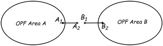
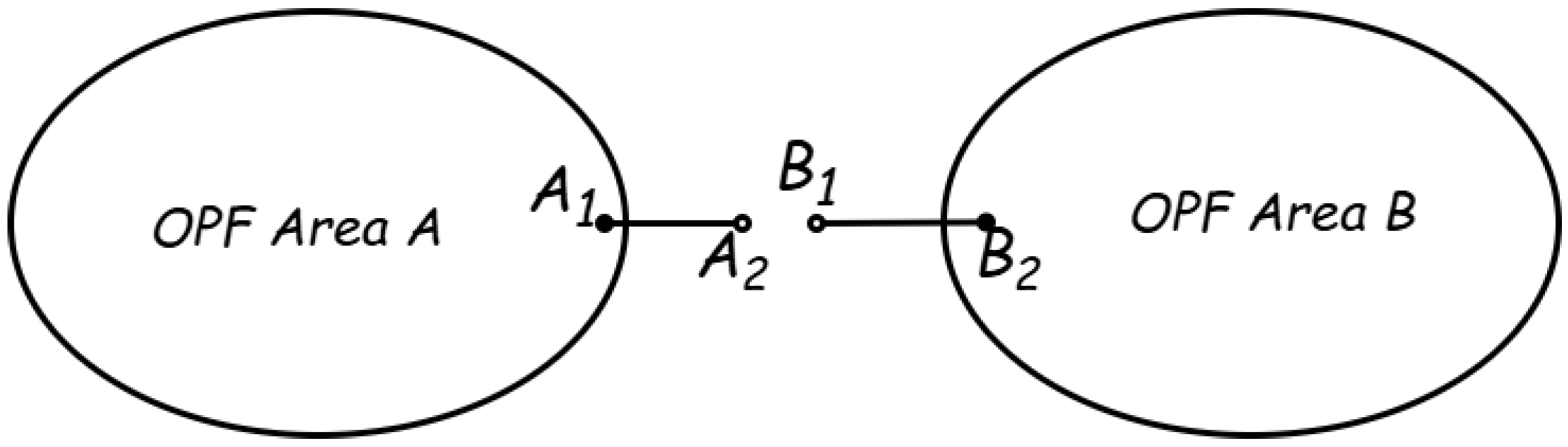
Area-based OPF decomposition reflects interconnected microgrids since they are geographically separated [53]. Here, we consider the decomposition of OPF into geographical areas as described in the work of Kim and Baldic [52]. The idea is to cut a tie-line connecting two areas and create a ‘dummy bus’ in one area and its copy in the other. On these buses, we assign duplicate shared variables such as the voltage and the phase angle. Figure 2 illustrates the area-based decomposition, in which the consensus is achieved by ensuring the equality of the variables at the dummy buses $A_2$ and $B_1$ in OPF area A and OPF area B, respectively. In addition, the power flow from bus $A_1$ to $A_2$ in OPF area A is equal to that from bus $B_1$ to $B_2$ in OPF area B.

Figure 2. Area-based decomposition of two interconnected power systems: two dummy generator buses at a tie-line connecting two areas, one at each area.

5.2. Source of Uncertainty in OPF

In this study, we consider the OPF under uncertainties in bus loads and photovoltaic (PV) generation forecasts in both areas. Bus loads, as well as renewable power generations, are usually considered known from various forecasting techniques. Here, we add a normally distributed error term on the estimated values to consider uncertainty. Although there have been studies on chance-constrained OPF [54], our focus is to study CCOPT of interconnected power systems.

5.3. Problem Formulation

We consider OPF of interconnected networks with linear model equations and quadratic objective function to minimize the cost of power generation by conventional generators. We assume a negligible tie-line resistance and a unit voltage magnitude at all buses [55]. To separate the OPF areas connected with a tie-line as described in Figure 2, the phase angle and power flow through the connecting buses remain as shared variables.

Let $n_{g_i}$, $n_{d_i}$, $n_{p{v}_i}$ and $n_{b_i}$ denote the number of generators, loads, PV systems and total buses in OPF area $i\in \mathcal{V}$, respectively. A general chance-constrained distributed optimal power flow (CCDOPF) problem is formulated as follows:

$$\begin{array}{cc}\hfill \underset{u}{min}& \sum _{i=1}^{N_s}{w}_i\left[\sum _{t=1}^{n_{b_i}}\left(a_{i_t}{p}_{g_{i_t}}^2+b_{i_t}{p}_{g_{i_t}}+c_{i_t}\right)\right]\hfill \end{array}$$

(48a)

$$\begin{array}{cc}\hfill \mathrm{s}.\mathrm{t}.& p_{g_{i_t}}+{\beta }_{i_t}{p}_{p{v}_{i_t}}-p_{d_{i_t}}-p_{i_{tl}}=0,\forall i\in \mathcal{V},\hfill \end{array}$$

(48b)

$$\begin{array}{cc}\hfill & p_{i_{tl}}={\displaystyle \frac{{\theta }_{i_t}-{\theta }_{i_l}}{X_{i_{tl}}}},\forall i\in \mathcal{V},\hfill \end{array}$$

(48c)

$$\begin{array}{cc}\hfill & \mathrm{Pr}\left\{p_{i_{tl}}^2\le P_{i_{tl}}^2\right\}\ge {\alpha }_i,\forall i\in \mathcal{V},\hfill \end{array}$$

(48d)

$$\begin{array}{cc}\hfill & \mathrm{Pr}\left\{p_{g_{i_{ref}}}\le P_{g_{i_{ref}}}\right\}\ge {\alpha }_i,\forall i\in \mathcal{V},\hfill \end{array}$$

(48e)

$$\begin{array}{cc}\hfill & \mathrm{Pr}\left\{p_{ij}^2\le P_{ij}^2\right\}\ge {\alpha }_{ij},\forall j:(i,j)\in \mathcal{E},\hfill \end{array}$$

(48f)

$$\begin{array}{cc}\hfill & \sum _{i=1}^{N_s}{A}_i{\left[p_{ij},{\theta }_{ij}\right]}^T=0,\forall j:(i,j)\in \mathcal{E},\hfill \end{array}$$

(48g)

$$\begin{array}{cc}\hfill & 0\le p_{g_{i_t}}\le P_{g_{i_t}},\forall i\in \mathcal{V},t\in \{1,\dots ,n_{b_i}\},\hfill \end{array}$$

(48h)

$$\begin{array}{cc}\hfill & 0\le {\beta }_{i_t}\le 1,\forall i\in \mathcal{V},t\in \{1,\dots ,n_{b_i}\}.\hfill \end{array}$$

(48i)

where $p_{g_{i_t}}$, $p_{p{v}_{i_t}}$ and $p_{d_{i_t}}$ denote the total thermal power generation, PV power generation and load demand at bus t in OPF area $i\in \mathcal{V}$, respectively. The variable ${\beta }_{i_t}$ denotes curtailment factor of the PV system at bus t in OPF area i, and ${\theta }_{i_k}$ the phase angle of bus at bus t in OPF area i. For brevity, variables $p_{ij}$ and ${\theta }_{ij}$ denote shared power flow and phase angle between OPF area i and j. Decoupling follows the discussion in Section 2.4 and Section 5.1. The parameter $P_{g_{i_t}}$ denotes the generation upper bound of the generator at bus t in OPF area i, while $P_{i_{tl}}$ denotes the capacity limit of the tie-line connecting buses t and l in area i and $X_{i_{kl}}$ the respective tie-line conductance. These parameters, as well as the economic data of thermal generators $a_{i_k}$, $b_{i_k}$, and $c_{i_k}$ in the objective function, are considered known by their respective subsystem $i\in \mathcal{V}$.

The local chance constraints (48d) and (48e) hold the internal power flows and reference generator output within its capacity at reliability level ${\alpha }_i$. The shared chance constraint (48f) enforces the tie-line capacity between areas at the compromised reliability level ${\alpha }_{ij}$. The conventional power generation $p_{g_{i_k}}$ and curtailment factor ${\beta }_{i_t}$ are bounded as (48h) and (48i).

In this problem, the control variables are the conventional power generation (with reference bus excluded) and curtailment factor, i.e., $u_i={[p_{g_{i_k}},{\beta }_{i_t}]}^T$. The state variables $x_i$ consist of power generation at the reference bus, phase angle, and power flow through buses, i.e., $x_i={[p_{g_{i_{ref}}},{\theta }_{i_t},p_{i_{tl}}]}^T$. The load demand and PV power generation forecasts are uncertain variables with a Gaussian forecasting error, i.e., ${\xi }_i={[{\xi }_{d_{i_t}},{\xi }_{p{v}_{i_t}}]}^T$, ${\xi }_i\in {\mathrm{\Omega }}_i\subset {\mathbb{R}}^{n_{d_i}+n_{p{v}_i}}$:

$$p_{d_{i_t}}={\widehat{p}}_{d_{i_t}}+{\xi }_{d_{i_t}}\mathrm{and}{p}_{p{v}_{i_t}}={\widehat{p}}_{p{v}_{i_t}}+{\xi }_{p{v}_{i_t}},$$

(49)

where ${\widehat{p}}_{d_{i_t}}$ and ${\widehat{p}}_{p{v}_{i_t}}$ are load-nominal demand and PV power generation forecasts, respectively.

5.4. Numerical Implementation

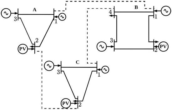
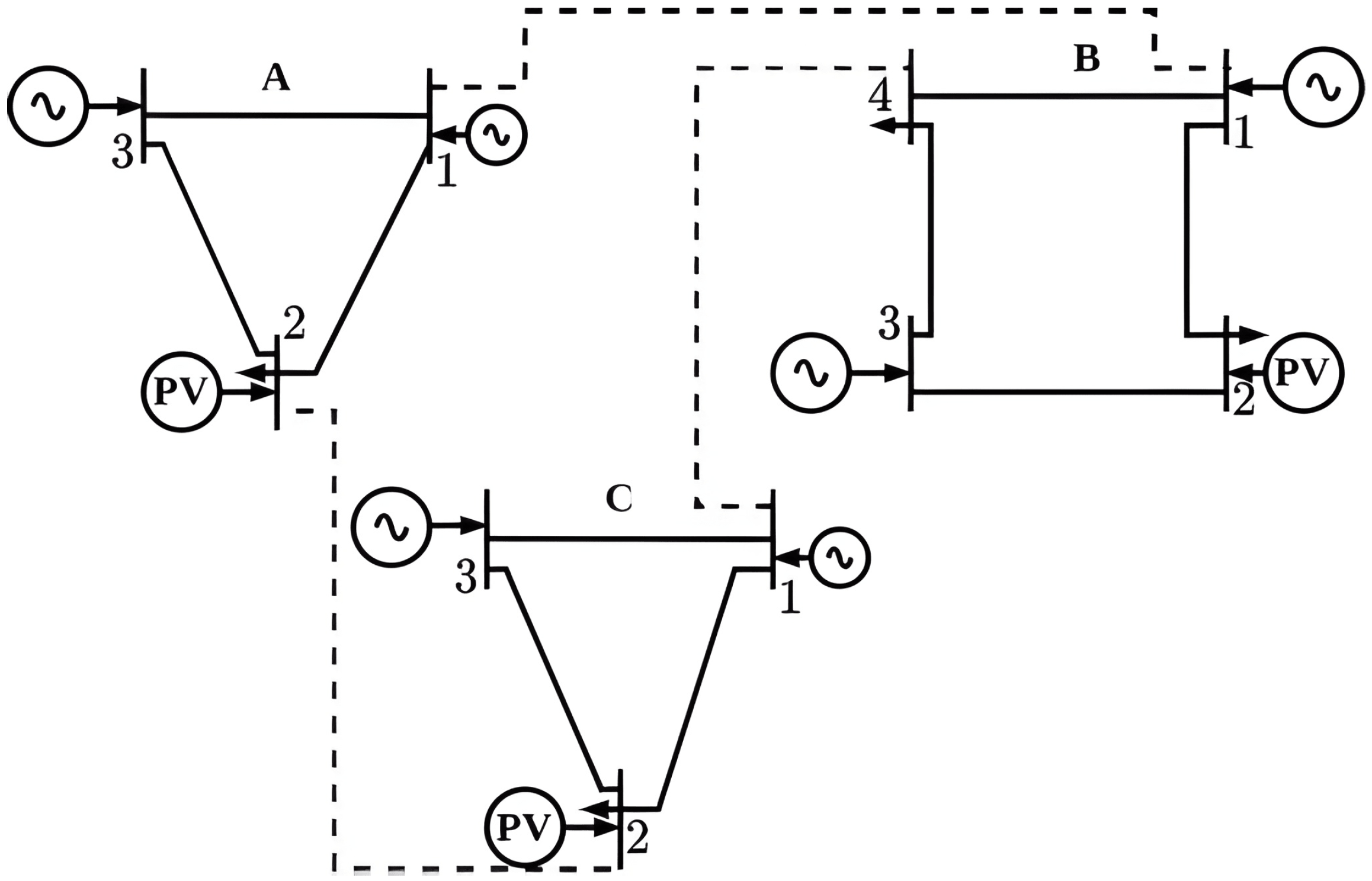
In this study, we implemented the proposed approach for OPF of three interconnected subsystems: a three-bus (OPF A), a four-bus (OPF B), and a three-bus (OPF C) system. The data of OPF A and OPF B are taken from [55], while OPF C uses a distinct three-bus design so that the three areas differ in economic data, network parameters, load, and PV installation. The interconnected system with the area-based decomposition is shown in Figure 3. The first computation was carried out in GAMS 33.2.0 with the IPOPT solver [56] (see Bussieck and Meeraus [57]) to solve the centralized inner–outer approximation problems. Then, we used ALADIN-$\alpha$ toolbox (Algorithm 2) [58] to implement the distributed optimization procedure.

Figure 3. Interconnected three-area system: connected pairwise through three tie-lines. Bus 3 in each area is the slack bus; tie-line boundaries are chosen on non-slack buses.

The uncertainty of the load demands and PV power generation are generated using Monte-Carlo sampling, which is used to evaluate both the expected cost in (29a) and (30a) and the smoothed probability functions in (27). Given the confidence level in Table 1, we use $M=1000$ samples to realize each load demand and PV power generation in all subsystems, yielding an accuracy of $\sigma \approx 4.2\times {10}^{-2}$ at the $95\%$ confidence level (cf. Remark 4). The parameter values used in the optimization problem are listed in Table 1. The smoothing function parameter values were chosen accordingly, with respect to the G-H function (25), and the ALADIN penalty parameters were set high to keep the feasibility of the solution.

Table 1. Optimization parameters.

Parameter	Description	Value
$1-\delta$	Confidence level	$0.95$
$\sigma$	Accuracy (from M, cf. Remark 4)	$4.2\times {10}^{-2}$
M	Sample size	1000
$\rho ,\mu$	ALADIN penalty parameters	${10}^3,{10}^4$
${\alpha }_1,{\alpha }_2,{\alpha }_3$	Reliability levels	$0.95,0.97,0.96$
$m_1,m_2$	Geletu–Hoffmann constants	$0.5,0.3$
${\gamma }_{12},{\gamma }_{13},{\gamma }_{23}$	Compromise weights on shared edges	$0.5,0.5,0.5$
$w_1,w_2,w_3$	Normalized Pareto weights (cf. (50))	$0.3368,0.3299,0.3333$

To consider conflicting reliability levels, we assume that OPF A, OPF B, and OPF C request ${\alpha }_1=0.95$, ${\alpha }_2=0.97$, and ${\alpha }_3=0.96$, respectively. We set the compromise weight ${\gamma }_{ij}=0.5$ on every shared edge $(i,j)\in \mathcal{E}$ in this study, which yields ${\alpha }_{12}=0.960$, ${\alpha }_{13}=0.955$, and ${\alpha }_{23}=0.965$. However, the weights in the objective function (48a) are set inversely proportional to the reliability levels and normalized to sum to one:

$$w_i={\displaystyle \frac{1/{\alpha }_i}{{\sum }_{j=1}^{N_s}1/{\alpha }_j}},\forall i\in \mathcal{V}.$$

(50)

After normalization via (14), this yields ${\overline{w}}_i>0$ with ${\sum }_i{\overline{w}}_i=1$, while penalizing subsystems with higher reliability demands.

Table 2 summarizes the data about the conventional generators, PV power generation and OPF systems. The tie-line capacity is considered to be equal for all inter-area tie-lines, while the tie-line conductance is the same within each subsystem. The economic data, as well as the system characteristics of OPF A and OPF B, are drawn from [55], and those of OPF C are set to differ so that the three subsystems are distinct. In addition, the tie-lines connecting the subsystems have their own characteristics. Bus 3 in each OPF system is considered the slack bus to set phase angle reference and balance the respective total power (see Figure 3).

Table 2. Optimization data for OPF problem.

Data	Description	Value
$a_{1_t},b_{1_t},c_{1_t}$	Economic data of thermal generators in A	$3.00,10.0,5.0$
$a_{2_t},b_{2_t},c_{2_t}$	Economic data of thermal generators in B	$4.05,11.0,7.0$
$a_{3_t},b_{3_t},c_{3_t}$	Economic data of thermal generators in C	$3.50,12.0,6.0$
${\widehat{p}}_{d_{1_2}}$	Load demand forecast in A	100 MW
${\widehat{p}}_{d_{2_2}},{\widehat{p}}_{d_{2_4}}$	Load demand forecasts in B	$100,25$ MW
${\widehat{p}}_{d_{3_2}}$	Load demand forecast in C	80 MW
${\widehat{p}}_{p{v}_{1_2}}$	PV power generation forecast in A	$45.0$ MW
${\widehat{p}}_{p{v}_{2_2}}$	PV power generation forecast in B	$50.0$ MW
${\widehat{p}}_{p{v}_{3_2}}$	PV power generation forecast in C	$55.0$ MW
$P_{g_{1_1}},P_{g_{1_3}}$	Thermal generation limits in A	$100,65$ MW
$P_{g_{2_1}},P_{g_{2_3}}$	Thermal generation limits in B	$100,65$ MW
$P_{g_{3_1}},P_{g_{3_3}}$	Thermal generation limits in C	$80,70$ MW
$P_{i_{tl}}$	Internal line capacity in each area	$50,50,45$ MW
$X_{1_{tl}},X_{2_{tl}},X_{3_{tl}}$	Tie-line conductance in A, B, C	$0.20,0.25,0.22$
$X_{ij}$	Conductance of each inter-area tie-line	$0.30$
$P_{ij}$	Capacity of inter-area tie-lines ($AB,AC,BC$)	$8,15,15$ MW

Although the present case study with three pairwise-coupled areas already addresses the conflicting-reliability mechanism on multiple shared edges, validation on larger and more diverse network topologies, including hypergraph extensions where a single state is shared among more than two subsystems, is left for future work.

5.5. Results and Discussion

This subsection presents the results and discussions for our system described above. All computations were carried out on a 64-bit Windows 10 Pro (version 22H2) machine equipped with an 11th Gen Intel(R) Core(TM) i7-1185G7 CPU @3.00 GHz (four cores, eight threads) and 16 GB of RAM.

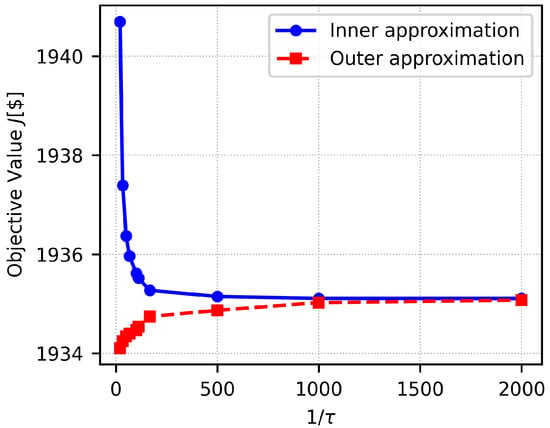
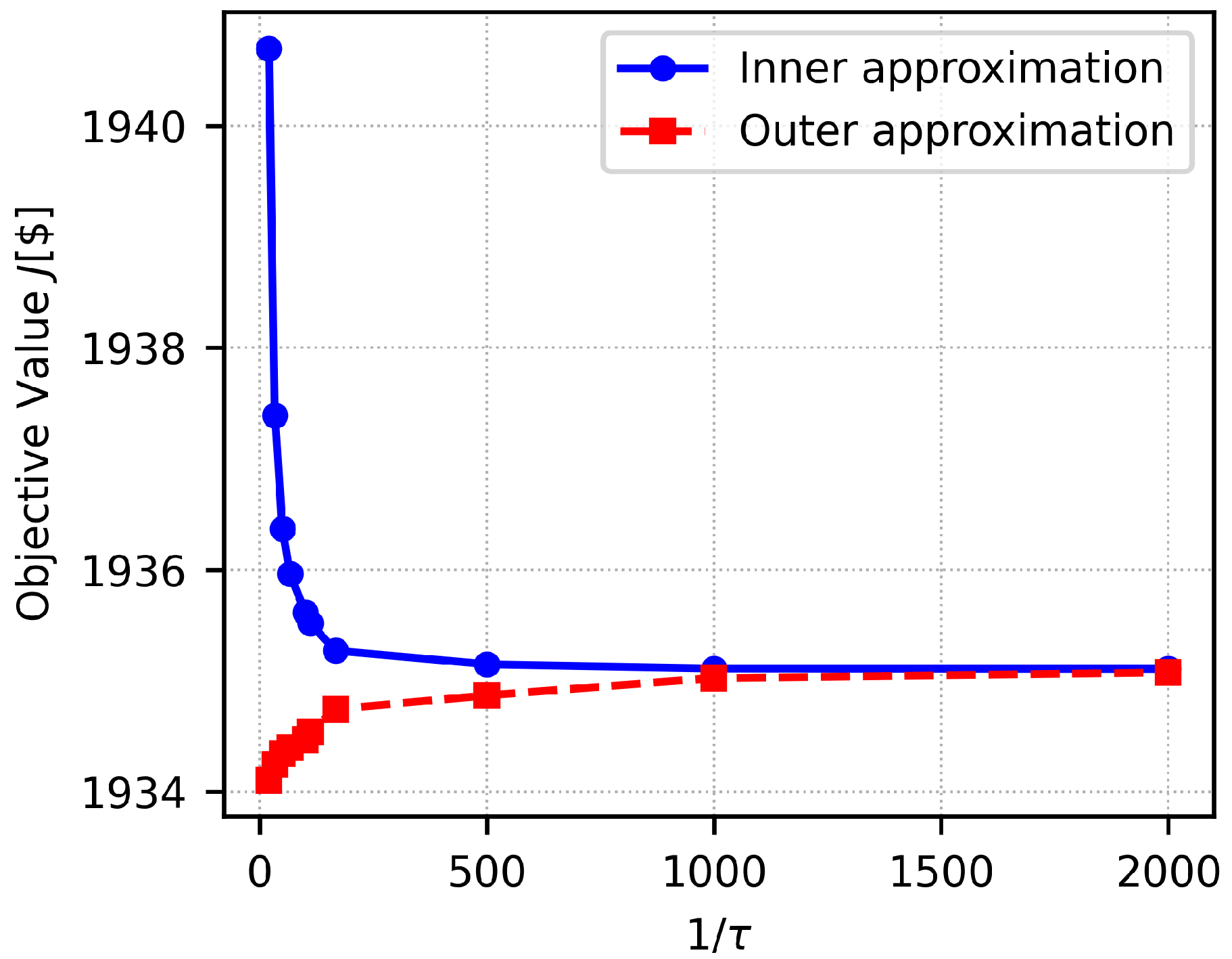
Figure 4 shows the convergence of the objective function values of the inner and outer approximation problems by gradually reducing the value of $\tau$. With the properties of inner–outer approximation approach, a solution of the inner approximation problem is considered as a solution of the chance-constrained solution due to its feasibility guarantee. The outer approximation problem provides a numerical stopping criterion for the smoothing parameter $\tau$. At $\tau =5\times {10}^{-4}$, the objective value difference reaches a sufficiently small value within our defined tolerance $tol$.

Figure 4. Objective function trajectory of the inner and outer approximation problems with a decreasing $\tau$.

To confirm that the smoothed approximations satisfy the intended chance constraints in practice, we evaluated the empirical tie-line feasibility frequencies on the three shared edges by Monte Carlo sampling at $\tau =5\times {10}^{-4}$ with 1000 samples. For the inner approximation, the frequencies on edges $(1,2)$, $(1,3)$, and $(2,3)$ are $0.963$, $0.961$, and $0.970$, respectively, all at or above the compromised reliability levels ${\alpha }_{12}=0.960$, ${\alpha }_{13}=0.955$, ${\alpha }_{23}=0.965$, confirming that the inner-approximation solution is feasible for the original chance-constrained problem and is near the true feasibility boundary, rather than over-conservative. For the outer approximation, the corresponding frequencies are $0.941$, $0.949$, and $0.932$, which—as expected—fall below the nominal targets on two of the three edges since the outer approximation is a relaxation. The inner and outer frequencies together bracket the true chance-constrained feasibility boundary, in agreement with the sandwich property [23].

Table 3 compares the proposed compromise rule against two baseline aggregation strategies that impose extreme uniform choices on the shared reliability levels. We solve the problem in three cases. In Case 1, each shared reliability level takes the lower of the two connected subsystems’ demands (${\alpha }_{ij}=min\{{\alpha }_i,{\alpha }_j\}$); in Case 2, each takes the higher (${\alpha }_{ij}=max\{{\alpha }_i,{\alpha }_j\}$); and in Case 3, each is defined from (3) with equal weights ${\gamma }_{ij}=0.5$. As predicted by Theorem 2, the total cost increases monotonically as the shared reliability levels are tightened, from $1934.92 in Case 1 to $1935.20 in Case 2, with Case 3 lying between the two. The per-subsystem allocations differ more visibly: across the three rules, $F_{1_{ia}}$ varies by about $8.84, $F_{2_{ia}}$ by $5.53, and $F_{3_{ia}}$ by $3.59. The reallocation has a clear physical interpretation: tightening the shared reliability levels restricts the export of cheap generation from OPF A across the tie-lines, so $F_{1_{ia}}$ decreases while $F_{2_{ia}}$ and $F_{3_{ia}}$ increase as OPF B and OPF C take on more of their own dispatch. The compromise rule in Case 3 sits between the two extreme rules and avoids the reliability dominance phenomenon described in Section 2, giving each subsystem a balanced share of the cost.

Table 3. Compromised reliability levels and corresponding inner-approximation objective values for the three subsystems with ${\alpha }_1=0.95$, ${\alpha }_2=0.97$, ${\alpha }_3=0.96$ at $\tau =5\times {10}^{-4}$.

Case	${\mathit{\alpha }}_{12}$	${\mathit{\alpha }}_{13}$	${\mathit{\alpha }}_{23}$	${\mathit{F}}_{1_{\mathit{ia}}}$ [$]	${\mathit{F}}_{2_{\mathit{ia}}}$ [$]	${\mathit{F}}_{3_{\mathit{ia}}}$ [$]	${\mathit{F}}_{\mathbf{total}}$ [$]
1	0.95	0.95	0.96	689.78	718.94	526.20	1934.92
2	0.97	0.96	0.97	680.94	724.47	529.79	1935.20
3	0.960	0.955	0.965	686.55	721.00	527.54	1935.09

The cost differences across the three cases are consistent with Theorem 2: the total cost increases monotonically as the shared reliability levels are tightened. Moving from Case 1 to Case 3 increases the total cost by approximately $\$6.82$, while moving from Case 3 to Case 2 increases it by approximately $\$5.61$. This reflects the tightening of the feasible sets at higher reliability levels, with a bounded marginal cost of reliability $L_{\tau }$ on the smoothed approximation problems.

To illustrate the robustness of the compromise to perturbations in the weights, we solved the inner approximation problem for several values of the compromise weight ${\gamma }_{12}$ on edge $(1,2)$, holding ${\gamma }_{13}$ and ${\gamma }_{23}$ fixed at $0.5$. This isolates a single pairwise weight and matches the setting of Corollary 2. Table 4 reports the resulting per-subsystem and total inner-approximation costs. As predicted by Theorem 2, the total cost is monotonically non-decreasing in ${\alpha }_{12}$, while the dependence on ${\gamma }_{12}$ is nearly linear, reflecting a fixed active set across the sweep. The endpoint slope gives an empirical Lipschitz constant of $L_{\tau }\approx 13.5$ $/unit reliability, so that the total-cost variation over the entire range ${\gamma }_{12}\in [0,1]$ is only about $0.27, well below $0.1\%$ of the total cost. Although the total cost is monotone, the individual subsystem costs redistribute in opposite directions: as ${\alpha }_{12}$ loosens, OPF A picks up more of the inter-area dispatch and its cost $F_{1_{ia}}$ increases, while OPF B and OPF C reduce their generation and $F_{2_{ia}}$, $F_{3_{ia}}$ decrease accordingly. The total cost decreases because A is the cheapest area at the margin. This confirms that the compromise is robust to moderate misspecification of the weights and that the shared chance constraint enables a meaningful but bounded reallocation of generation across the three areas.

Table 4. Sensitivity of the inner-approximation costs to the compromise weight ${\gamma }_{12}$ on edge $(1,2)$, with ${\gamma }_{13}={\gamma }_{23}=0.5$ held fixed. All values computed with $M=1000$ samples at $\tau =5\times {10}^{-4}$.

${\mathit{\gamma }}_{12}$	${\mathit{\alpha }}_{12}$	${\mathit{F}}_{1_{\mathit{ia}}}$ [$]	${\mathit{F}}_{2_{\mathit{ia}}}$ [$]	${\mathit{F}}_{3_{\mathit{ia}}}$ [$]	${\mathit{F}}_{\mathbf{total}}$ [$]
0.00	0.970	680.96	724.49	529.82	1935.27
0.25	0.965	684.23	722.44	528.48	1935.15
0.50	0.960	686.55	721.00	527.54	1935.09
0.75	0.955	688.35	719.89	526.80	1935.04
1.00	0.950	689.81	718.98	526.21	1935.00

As seen in Table 5, the computation time taken to solve the problem using the ALADIN-$\alpha$ toolbox increases with a reducing $\tau$, reflecting the increased computational efforts for the solution at a smaller value of $\tau$. This is due to the fact that using a smaller value $\tau$ leads to the parametric smoothing function near zero that can result in a vanishing gradient. We addressed this issue by using an increased sample size as well as taking the solution from a previous $\tau$ as the initial guess for the next iteration.

Table 5. Computation time in seconds of inner and outer approximation problems with reducing $\tau$.

$\mathit{\tau }$	$5\times {10}^{-2}$	${10}^{-2}$	$5\times {10}^{-3}$	${10}^{-3}$	$5\times {10}^{-4}$
IA	6.19	8.70	12.04	20.23	29.71
OA	2.11	3.91	4.03	5.56	7.90

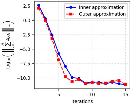
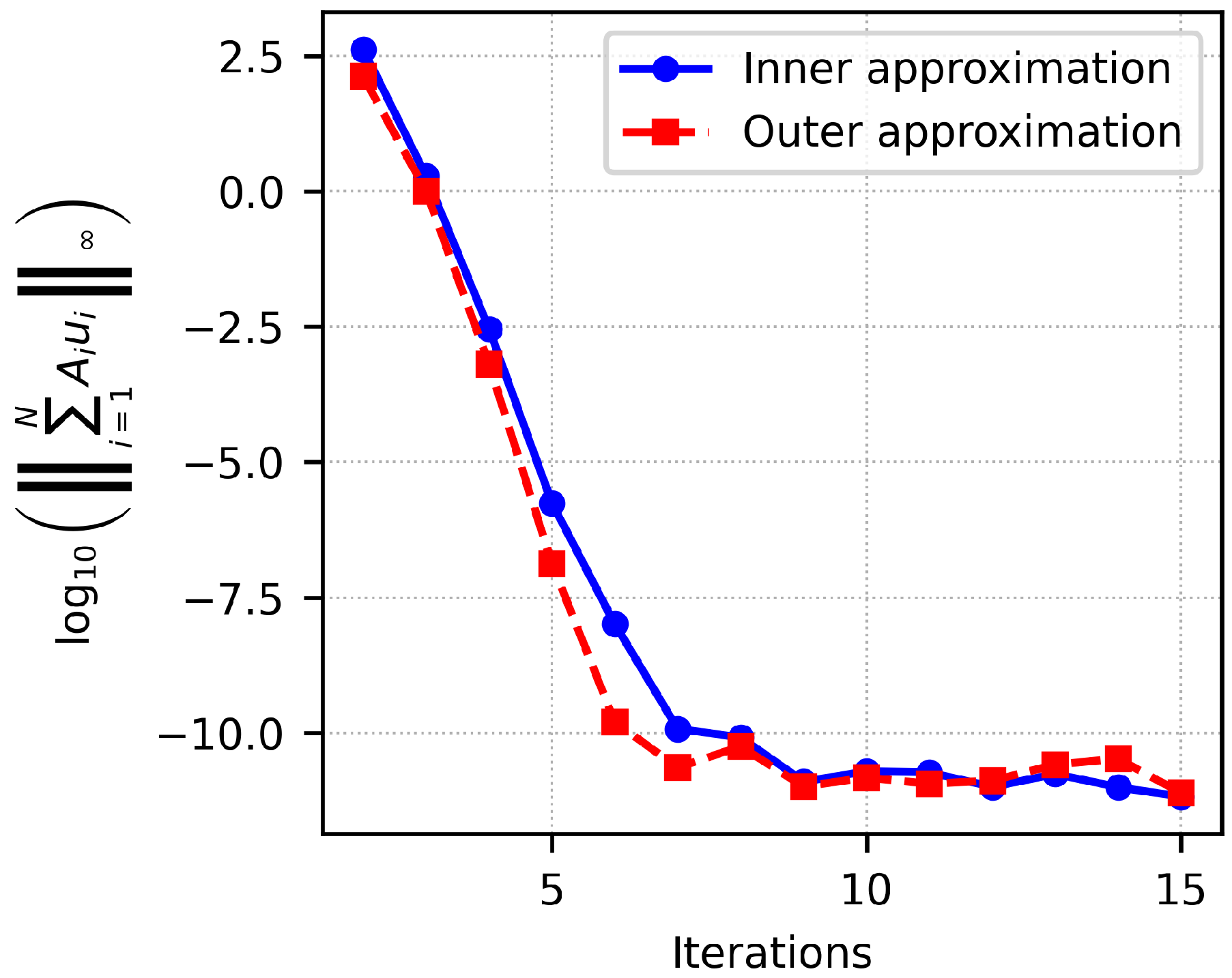
Given the optimal value of the smoothing parameter $\tau =5\times {10}^{-4}$, the two smoothing approximation problems were solved with the ALADIN Algorithm 2. The penalty parameters $\rho$ and $\mu$ were set high (see Table 1) to ensure convergence and feasibility, respectively. Figure 5 shows the ALADIN iterations of both smoothing problems, reflecting the convergence of the feasible sets and optimal objective values of (IADOPT)_τ and (OADOPT)_τ as $\tau$ tends to zero.

Figure 5. Consensus violation for inner and outer approximations over iterations with $\tau =5\times {10}^{-4}$.

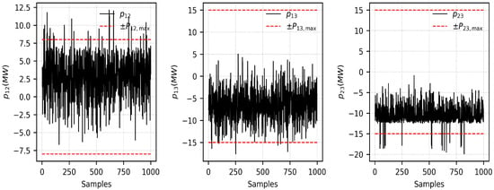
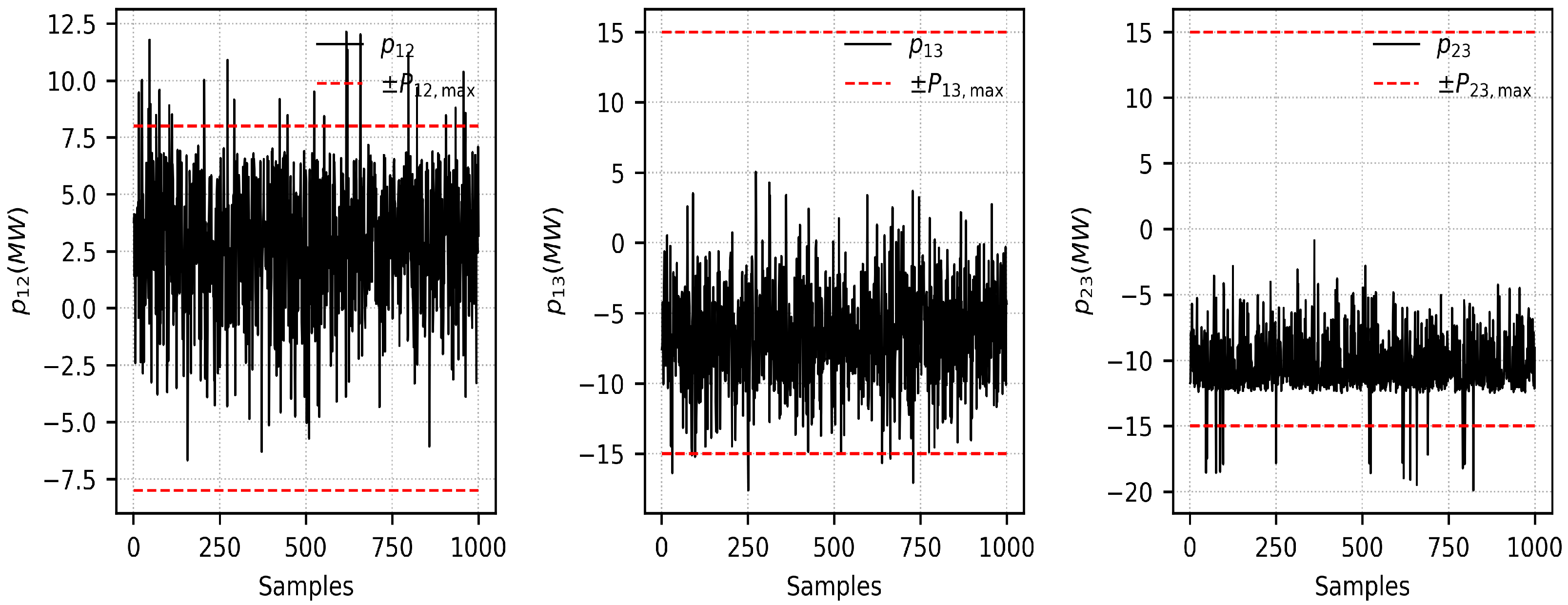
Figure 6 shows the sample-wise power exchanges on the three tie-lines connecting OPF systems A, B, and C at the optimal smoothing parameter. Each exchange is kept within its tie-line capacity in most realizations, with a small fraction of violations consistent with the compromised reliability levels of the shared chance constraints. Based on (48g) and the size of realizations of the random variables, each shared power flow has the dimension M. The size of the equality coupling constraint linearly increases with M, necessitating an efficient parallel computation of the centralized problem (46). Although the size of the smoothing problems (IADOPT)_τ (29) and (OADOPT)_τ (30) increase with the sample size, they are highly parallelizable, as the Hessian approximations $H_i$ and coupling matrices $A_i$ for the interconnected systems $i\in \mathcal{V}$ are block matrices.

Figure 6. Sample-wise inter-area power exchanges $p_{12}$, $p_{13}$, and $p_{23}$ between OPF systems A, B, and C at $\tau =5\times {10}^{-4}$. The dashed red lines indicate the corresponding tie-line capacity limits.

The computation times taken for solving the inner and outer approximation problems with the ALADIN Algorithm 2 in Python 3 with CasADi [59] at $\tau =5\times {10}^{-4}$ are $7.13$ and $5.04$ h, respectively. Here, there is a high potential to enhance the computational efficiency by exploiting the problem structure and using a parallel implementation.

6. Conclusions

A solution approach to chance-constrained distributed optimization for interconnected systems with shared states under uncertainty has been proposed. The chance-constrained formulation gives each subsystem the flexibility to hold operational constraints with a self-defined reliability level, which introduces conflicting reliability requirements on the shared state. We have proposed a method for compromising the reliability level through a weighted average approach. In addition, we established the Lipschitz continuity of the optimal cost with respect to the compromised reliability level for the smoothed approximation problems, providing a theoretical basis for evaluating the cost of the compromise. To enhance the fairness among the interconnected systems, their objective functions are weighted to balance the trade-offs, with normalized inverse-reliability weights ensuring the consistency of the formulation. Furthermore, we extended our recently proposed inner–outer approximation approach to address the intractability and non-smoothness of chance constraints in the distributed setting. We determined the sample size for multidimensional integral computation using the concentration inequalities. Finally, we used the ALADIN algorithm to solve the resulting nonlinear optimization problems in a distributed way. The proposed method was tested on an interconnected optimal power flow problem with three subsystems.

Future studies include a further analysis of uncertainty cascading between interconnected systems and extending the fairness analysis in specific interconnected systems under uncertainty. The parallel implementation framework, as well as extending the results to dynamical systems, will also be the main focus of our future research. An extension to nonlinear system models, which would require handling nonlinear coupling structures within the ALADIN framework, and larger-scale networks with comparisons to baseline approaches, such as scenario-based and robust optimization methods, are also planned. Practical deployment aspects, such as communication delays, parallel implementation efficiency, and integration with the existing energy management infrastructure, are also part of our planned future research, building on the inherently parallelizable block structure of the ALADIN-based decomposition developed in this study.

References

- Camponogara, E.; Jia, D.; Krogh, B.H.; Talukdar, S. Distributed model predictive control. IEEE Control Syst. Mag. 2002, 22, 44–52. [Google Scholar] [CrossRef] [Scilit]
- Stewart, B.T.; Venkat, A.N.; Rawlings, J.B.; Wright, S.J.; Pannocchia, G. Cooperative distributed model predictive control. Syst. Control Lett. 2010, 59, 460–469. [Google Scholar] [CrossRef] [Scilit]
- Campion, M.; Ranganathan, P.; Faruque, S. UAV swarm communication and control architectures: A review. J. Unmanned Veh. Syst. 2018, 7, 93–106. [Google Scholar] [CrossRef] [Scilit]
- Housh, M.; Ohar, Z. Model-based approach for cyber-physical attack detection in water distribution systems. Water Res. 2018, 139, 132–143. [Google Scholar] [CrossRef] [Scilit]
- Reilly, J.; Bayen, A.M. Distributed optimization for shared state systems: Applications to decentralized freeway control via subnetwork splitting. IEEE Trans. Intell. Transp. Syst. 2015, 16, 3465–3472. [Google Scholar] [CrossRef] [Scilit]
- Geletu, A.; Klöppel, M.; Zhang, H.; Li, P. Advances and applications of chance-constrained approaches to systems optimisation under uncertainty. Int. J. Syst. Sci. 2013, 44, 1209–1232. [Google Scholar] [CrossRef] [Scilit]
- Roald, L.A.; Pozo, D.; Papavasiliou, A.; Molzahn, D.K.; Kazempour, J.; Conejo, A. Power systems optimization under uncertainty: A review of methods and applications. Electr. Power Syst. Res. 2023, 214, 108725. [Google Scholar] [CrossRef] [Scilit]
- Choudhury, S.; Gupta, J.K.; Kochenderfer, M.J.; Sadigh, D.; Bohg, J. Dynamic multi-robot task allocation under uncertainty and temporal constraints. Auton. Robot. 2022, 46, 231–247. [Google Scholar] [CrossRef] [Scilit]
- Wang, W.; Long, J.; Wen, C.; Huang, J. Recent advances in distributed adaptive consensus control of uncertain nonlinear multi-agent systems. J. Control Decis. 2020, 7, 44–63. [Google Scholar] [CrossRef] [Scilit]
- Zio, E.; Sansavini, G. Modeling cascading failures in “systems of systems” with uncertain behavior. In Proceedings of the ICASP11, Zurich, Switzerland, 1–4 August 2011; pp. 1858–1866. Available online: https://centralesupelec.hal.science/hal-00658101v1 (accessed on 1 April 2026).
- Everett, H., III. Generalized Lagrange multiplier method for solving problems of optimum allocation of resources. Oper. Res. 1963, 11, 399–417. [Google Scholar] [CrossRef] [Scilit]
- Boyd, S.; Parikh, N.; Chu, E.; Peleato, B.; Eckstein, J. Distributed optimization and statistical learning via the alternating direction method of multipliers. Found. Trends® Mach. Learn. 2011, 3, 1–122. [Google Scholar] [CrossRef] [Scilit]
- Houska, B.; Frasch, J.; Diehl, M. An augmented Lagrangian based algorithm for distributed nonconvex optimization. SIAM J. Optim. 2016, 26, 1101–1127. [Google Scholar] [CrossRef] [Scilit]
- Dantzig, G.B. Linear programming under uncertainty. Manag. Sci. 1955, 1, 197–206. [Google Scholar] [CrossRef] [Scilit]
- Conejo, A.J.; Wu, X. Robust optimization in power systems: A tutorial overview. Optim. Eng. 2022, 23, 2051–2073. [Google Scholar] [CrossRef] [Scilit]
- Lima, R.M.; Conejo, A.J.; Giraldi, L.; Le Maître, O.; Hoteit, I.; Knio, O.M. Sample average approximation for risk-averse problems: A virtual power plant scheduling application. EURO J. Comput. Optim. 2021, 9, 100005. [Google Scholar] [CrossRef] [Scilit]
- Charnes, A.; Cooper, W.W. Chance-constrained programming. Manag. Sci. 1959, 6, 73–79. [Google Scholar] [CrossRef] [Scilit]
- Li, P.; Arellano-Garcia, H.; Wozny, G. Chance constrained programming approach to process optimization under uncertainty. Comput. Chem. Eng. 2008, 32, 25–45. [Google Scholar] [CrossRef] [Scilit]
- El Shamy, A.R.; Aduama, P.; Al-Sumaiti, A.S. Chance constrained optimal sizing of a hybrid PV/battery/hydrogen isolated microgrid: A life-cycle analysis. Energy Convers. Manag. 2025, 332, 119707. [Google Scholar] [CrossRef] [Scilit]
- Chacko, K.; Alizadeh, M.; Capitanescu, F.; Li, P. Chance constrained AC security constrained optimal power flow via the inner-outer approximation algorithm. IEEE Trans. Ind. Appl. 2025, 1–11. [Google Scholar] [CrossRef] [Scilit]
- Wendt, M.; Li, P.; Wozny, G. Nonlinear chance-constrained process optimization under uncertainty. Ind. Eng. Chem. Res. 2002, 41, 3621–3629. [Google Scholar] [CrossRef] [Scilit]
- van Ackooij, W. Eventual convexity of chance constrained feasible sets. Optimization 2015, 64, 1263–1284. [Google Scholar] [CrossRef] [Scilit]
- Geletu, A.; Hoffmann, A.; Kloppel, M.; Li, P. An inner-outer approximation approach to chance constrained optimization. SIAM J. Optim. 2017, 27, 1834–1857. [Google Scholar] [CrossRef] [Scilit]
- Geletu, A.; Klöppel, M.; Hoffmann, A.; Li, P. A tractable approximation of non-convex chance constrained optimization with non-Gaussian uncertainties. Eng. Optim. 2015, 47, 495–520. [Google Scholar] [CrossRef] [Scilit]
- Voropai, R.; Geletu, A.; Li, P. Model Predictive Control of Parabolic PDE Systems under Chance Constraints. Mathematics 2023, 11, 1372. [Google Scholar] [CrossRef] [Scilit]
- Kunya, A.B.; Abubakar, A.S.; Yusuf, S.S. Review of economic dispatch in multi-area power system: State-of-the-art and future prospective. Electr. Power Syst. Res. 2023, 217, 109089. [Google Scholar] [CrossRef] [Scilit]
- Molzahn, D.K.; Dörfler, F.; Sandberg, H.; Low, S.H.; Chakrabarti, S.; Baldick, R.; Lavaei, J. A survey of distributed optimization and control algorithms for electric power systems. IEEE Trans. Smart Grid 2017, 8, 2941–2962. [Google Scholar] [CrossRef] [Scilit]
- Al-Saffar, M.; Musilek, P. Distributed optimization for distribution grids with stochastic der using multi-agent deep reinforcement learning. IEEE Access 2021, 9, 63059–63072. [Google Scholar] [CrossRef] [Scilit]
- Lyons, D.; Calliess, J.P.; Hanebeck, U.D. Chance constrained model predictive control for multi-agent systems with coupling constraints. In Proceedings of the 2012 American Control Conference (ACC); IEEE: Piscataway, NJ, USA, 2012; pp. 1223–1230. [Google Scholar] [CrossRef] [Scilit]
- Zhai, J.; Jiang, Y.; Shi, Y.; Jones, C.N.; Zhang, X.P. Distributionally robust joint chance-constrained dispatch for integrated transmission-distribution systems via distributed optimization. IEEE Trans. Smart Grid 2022, 13, 2132–2147. [Google Scholar] [CrossRef] [Scilit]
- Chen, X.; Zhai, J.; Shen, J.; Wang, Q.; Li, S.; Wang, S. Distributed and distributionally robust chance-constrained scheduling for VSC-MTDC meshed AC/DC power networks. IEEE Trans. Netw. Sci. Eng. 2024, 11, 3317–3331. [Google Scholar] [CrossRef] [Scilit]
- Abdelaziz, F.B. Solution approaches for the multiobjective stochastic programming. Eur. J. Oper. Res. 2012, 216, 1–16. [Google Scholar] [CrossRef] [Scilit]
- Gutjahr, W.J.; Pichler, A. Stochastic multi-objective optimization: A survey on non-scalarizing methods. Ann. Oper. Res. 2016, 236, 475–499. [Google Scholar] [CrossRef] [Scilit]
- Hu, M.; Cho, H. A probability constrained multi-objective optimization model for CCHP system operation decision support. Appl. Energy 2014, 116, 230–242. [Google Scholar] [CrossRef] [Scilit]
- Mugenga, I.R.; Geletu, A.; Li, P. Chance Constrained Distributed Optimisation for Interconnected Power Systems. IFAC-PapersOnLine 2024, 58, 128–133. [Google Scholar] [CrossRef] [Scilit]
- Dai, L.; Xia, Y.; Gao, Y. Distributed model predictive control of linear systems with stochastic parametric uncertainties and coupled probabilistic constraints. SIAM J. Control Optim. 2015, 53, 3411–3431. [Google Scholar] [CrossRef] [Scilit]
- Nedić, A.; Liu, J. Distributed optimization for control. Annu. Rev. Control Robot. Auton. Syst. 2018, 1, 77–103. [Google Scholar] [CrossRef] [Scilit]
- Wu, B.; Peng, Z.; Wen, G.; Yang, S.; Huang, T. Distributed coupling chance-constraint optimization under unknown uncertainty distributions. IEEE Trans. Control Netw. Syst. 2024, 11, 1692–1703. [Google Scholar] [CrossRef] [Scilit]
- Yadollahi, S.S.; Kebriaei, H.; Soudjani, S. Stochastic generalized dynamic games with coupled chance constraints. arXiv 2025, arXiv:2501.02279. [Google Scholar] [CrossRef] [Scilit]
- Marler, R.T.; Arora, J.S. Survey of multi-objective optimization methods for engineering. Struct. Multidiscip. Optim. 2004, 26, 369–395. [Google Scholar] [CrossRef] [Scilit]
- Yadollahi, S.; Kebriaei, H.; Soudjani, S. Generalized stochastic dynamic aggregative game for demand-side management in microgrids with shared battery. IEEE Control. Syst. Lett. 2023, 7, 3429–3434. [Google Scholar] [CrossRef] [Scilit]
- Marshall, A.W.; Olkin, I.; Arnold, B.C. Inequalities: Theory of Majorization and Its Applications, 2nd ed.; Springer Series in Statistics; Springer: New York, NY, USA, 2011. [Google Scholar] [CrossRef] [Scilit]
- Hansen, F.; Pedersen, G.K. Jensen’s operator inequality. Bull. Lond. Math. Soc. 2003, 35, 553–564. [Google Scholar] [CrossRef] [Scilit]
- Krantz, S.G.; Parks, H.R. The Implicit Function Theorem: History, Theory, and Applications; Springer Science & Business Media: Berlin/Heidelberg, Germany, 2002. [Google Scholar] [CrossRef] [Scilit]
- Gauvin, J. A necessary and sufficient regularity condition to have bounded multipliers in nonconvex programming. Math. Program. 1977, 12, 136–138. [Google Scholar] [CrossRef] [Scilit]
- Bonnans, J.F.; Shapiro, A. Perturbation Analysis of Optimization Problems; Springer Science & Business Media: Berlin/Heidelberg, Germany, 2013. [Google Scholar] [CrossRef] [Scilit]
- Hsu, P.L.; Robbins, H. Complete convergence and the law of large numbers. Proc. Natl. Acad. Sci. USA 1947, 33, 25–31. [Google Scholar] [CrossRef] [Scilit]
- Hoeffding, W. Probability inequalities for sums of bounded random variables. In The Collected Works of Wassily Hoeffding; Springer: New York, NY, USA, 1994; pp. 409–426. [Google Scholar] [CrossRef]
- Carpentier, J. Contribution to the economic dispatch problem. Bull. Soc. Fr. Electr. 1962, 3, 431–447. [Google Scholar]
- Pacaud, F.; Maldonado, D.A.; Shin, S.; Schanen, M.; Anitescu, M. A feasible reduced space method for real-time optimal power flow. Electr. Power Syst. Res. 2022, 212, 108268. [Google Scholar] [CrossRef] [Scilit]
- Gbadega, P.A.; Sun, Y.; Balogun, O.A. A unified optimization framework for cost-effective and voltage-stable operation of renewable energy-based microgrids using mixed-integer nonlinear programming. E-Prime Electr. Eng. Electron. Energy 2025, 12, 101010. [Google Scholar] [CrossRef] [Scilit]
- Kim, B.H.; Baldick, R. Coarse-grained distributed optimal power flow. IEEE Trans. Power Syst. 1997, 12, 932–939. [Google Scholar] [CrossRef] [Scilit]
- Britton, J.P. Improved area interchange control for Newton’s method load flows. IEEE Trans. Power Appar. Syst. 1969, 10, 1577–1581. [Google Scholar] [CrossRef]
- Zhang, H.; Li, P. Chance constrained programming for optimal power flow under uncertainty. IEEE Trans. Power Syst. 2011, 26, 2417–2424. [Google Scholar] [CrossRef] [Scilit]
- Soroudi, A. Power System Optimization Modeling in GAMS; Springer: Berlin/Heidelberg, Germany, 2017; Volume 78. [Google Scholar] [CrossRef] [Scilit]
- Wächter, A.; Biegler, L.T. On the implementation of an interior-point filter line-search algorithm for large-scale nonlinear programming. Math. Program. 2006, 106, 25–57. [Google Scholar] [CrossRef] [Scilit]
- Bussieck, M.R.; Meeraus, A. General algebraic modeling system (GAMS). In Modeling Languages in Mathematical Optimization; Springer: Berlin/Heidelberg, Germany, 2004; pp. 137–157. [Google Scholar] [CrossRef] [Scilit]
- Engelmann, A.; Jiang, Y.; Benner, H.; Ou, R.; Houska, B.; Faulwasser, T. ALADIN—An open-source MATLAB toolbox for distributed non-convex optimization. Optim. Control Appl. Methods 2022, 43, 4–22. [Google Scholar] [CrossRef] [Scilit]
- Andersson, J.; Gillis, J.; Horn, G.; Rawlings, J.; Diehl, M. CasADi—A software framework for nonlinear optimization and optimal control. Math. Program. Comput. 2018, 11, 1–36. [Google Scholar] [CrossRef] [Scilit]
Disclaimer/Publisher’s Note: The statements, opinions and data contained in all publications are solely those of the individual author(s) and contributor(s) and not of MDPI and/or the editor(s). MDPI and/or the editor(s) disclaim responsibility for any injury to people or property resulting from any ideas, methods, instructions or products referred to in the content. |
© 2026 by the authors. Licensee MDPI, Basel, Switzerland. This article is an open access article distributed under the terms and conditions of the Creative Commons Attribution (CC BY) license.