A Study of King-Type Operators Connecting Wavelet and Quantum Calculus: Numerical and Graphical Analysis

Abstract

This paper introduces a new class of King-type wavelet-assisted Kantorovich q-Baskakov operators, built to address the observation that classical operators of this type typically fail to reproduce the quadratic test function exactly. Moment formulas are derived for these operators, and a weighted Korovkin-type theorem is used to establish convergence. The speed of pointwise convergence is then quantified with the help of the modulus of smoothness and Lipschitz-type maximal function spaces; the resulting convergence factor ${\delta }_n^{q_n}$ turns out to be smaller than that reported for earlier q-Baskakov constructions, indicating an improvement in approximation power. Beyond the theoretical development, a numerical and graphical investigation plots the pointwise error $|{\mathrm{Y}}_{n,q}^{*}f\left(z\right)-f\left(z\right)|$ for several parameter pairs $(n,q)$, with the error found to decrease steadily as n increases and q approaches 1, consistent with the theoretical estimates. Implementation details accompany this study to make the computations reproducible and to connect the abstract approximation-theoretic results with their practical execution.

1. Introduction and Preliminaries

A large number of positive linear operator sequences are constructed so as to reproduce the constant and linear test functions exactly; that is, $L(e_i,y)=e_i\left(y\right)$ for $i=0,1$ where $e_i\left(y\right)=y^i$; the Bernstein, Baskakov, Szász–Mirakjan, and Phillips families are all examples of this behavior. What none of these classical constructions manages, however, is an exact reproduction of the second-degree monomial $e_2$, so that in general $L_m(e_2,y)\ne e_2\left(y\right)$. It was King [1] who first repaired this gap, proposing a re-parametrization scheme under which the quadratic test function is left invariant. When this device is applied to the Bernstein polynomials, it produces the modified operator

$$B_m^{*}(h;y)={\displaystyle \sum _{j=0}^m}\left({\displaystyle \genfrac{}{}{0pt}{}{m}{j}}\right){\left({\gamma }_m^{*}\left(y\right)\right)}^j{(1-{\gamma }_m^{*}\left(y\right))}^{m-j}h\left({\displaystyle \frac{j}{m}}\right),$$

with $y,{\gamma }_m^{*}\left(y\right)\in [0,1]$, $m=1,2,3,...$, where ${\gamma }_m^{*}\left(y\right)$ is given by

$${\gamma }_m^{*}\left(y\right)=\left\{\begin{array}{c}-{\displaystyle \frac{1}{2(m-1)}}+\sqrt{\left({\displaystyle \frac{m}{m-1}}\right)y^2+{\displaystyle \frac{1}{4(m-1)}}}\mathrm{for}m=2,3,4,...\hfill \\ y^2,\mathrm{for}m=1.\hfill \end{array}\right.$$

The construction $B_m^{*}(h;y)$ above is a re-parametrization of the classical Bernstein polynomial $B_m(h;y)={\sum }_{j=0}^m\left({\displaystyle \genfrac{}{}{0pt}{}{m}{j}}\right)y^j{(1-y)}^{m-j}h(j/m)$, going back to Bernstein’s original probabilistic proof of the Weierstrass approximation theorem [2]: replacing the argument y of the classical binomial weights by King’s function ${\gamma }_m^{*}\left(y\right)$ leaves the operator positive and linear, changes nothing about $e_0$ and, because ${\gamma }_m^{*}\left(y\right)$ is chosen precisely so that $B_m^{*}(e_2;y)=y^2$, repairs the one test function that the classical Bernstein polynomials do not reproduce exactly. Every operator considered later in this paper—the q-Baskakov family ${\mathsf{\Gamma }}_{n,q}$ of [3], its Kantorovich modification with a scaling kernel, and the King-type operator ${\mathrm{Y}}_{n,q}^{*}$ built from it—inherits this same re-parametrization idea, so that the present construction sits at the intersection of three classical threads in approximation theory: the Bernstein–Baskakov family of positive linear operators [2,4], King’s second-moment-preserving re-parametrization [1], and the general Korovkin-type convergence theory that governs when such operator sequences converge at all (see, e.g., [5] and Section 3.2 below). King [1] showed that, restricted to $0\le y\le {\displaystyle \frac{1}{3}}$, his operators $B_m^{*}(h;y)$ outperform the classical Bernstein construction analyzed by Lupas [4]. Extending this idea further, Doğru and Örkcü [6] constructed King-type analogues of the Meyer–König–Zeller operators along with their q-versions, achieving sharper error bounds than both the classical and q-based Meyer–König–Zeller families. Along similar lines, Yilmaz et al. [7] examined King-type Baskakov operators centered on the test functions $e_0$ and $e^{2ax}$ for a fixed positive constant a, uncovering shape-preservation results tied to generalized convexity. The King methodology has since been carried over to many other operator families with their own approximation properties studied case by case; representative instances appear in [8,9,10].

Over recent years, quantum calculus has emerged as a fruitful setting in which to build and analyze positive linear operators; representative studies include [11,12,13,14,15]. More broadly, the design and tuning of structured operators is also an active theme outside classical approximation theory: He et al. [16] propose a model-based approach to accelerate the tuning of deep-network operators, underscoring the practical value of operator constructions whose parameters (here, our n and q) can be chosen to control performance in a predictable way, and Li et al. [17] develop a permutation-based method for generating mass functions that captures class bias through structured combinatorial transformations, a construction philosophy—building a new operator from an existing one via a controlled, invertible transformation—that parallels the King-type re-parametrization used throughout the present paper. These connections suggest that operator-tuning ideas developed in approximation theory and in applied/data-driven settings can inform one another. Because the Kantorovich q-Baskakov operators with scaling kernels fail to preserve the second moment $e_2$, the present work is aimed at constructing a King-type analogue of this family and examining how well it approximates. Related constructions built on kernel ideas can be found in [18,19,20,21,22,23,24]. More recently, this trend has expanded to include parametric and generalized constructions, with Nasiruzzaman and Alotaibi [25] developing a Kantorovich extension of the parametric generalized q-Schurer operators and investigating their approximation properties. We first record several preliminary facts that will be used later on.

Throughout this paper, quantum calculus refers to the Jackson q-calculus that underlies the entire construction–the q-integers ${\left[n\right]}_q$, the q-binomial coefficients, the q-Pochhammer symbol ${(1+·)}_q^n$, and the associated q-integral and not to quantum computing or quantum information processing; no claim of a quantum-computational application is made or intended anywhere in what follows, and any phrasing that might be read otherwise is not so intended. Wavelet, for its part, refers to the nonnegative compactly supported scaling kernel $\mathsf{\Psi }$ introduced in Section 2, which plays a role analogous to that of a scaling function in a multiresolution analysis [26,27,28]: it localizes and redistributes the mass of each Kantorovich-type average over a compact window, in the spirit of the wavelet-assisted Kantorovich operators of [18,19,20,21,24]. Unlike a genuine wavelet basis, $\mathsf{\Psi }$ is not required to oscillate in sign or to annihilate higher-order moments (Remark 1 below); the wavelet connection therefore sits at the level of the kernel-based construction technique common to that line of work, rather than a full multiresolution decomposition. What distinguishes ${\mathrm{Y}}_{n,q}^{*}$ from all of [18,19,20,21,24] as well as from the classical construction of [3] is the King-type re-parametrization introduced in Section 2: none of those wavelet-Kantorovich or classical q-Baskakov operators reproduces the quadratic test function $e_2$ exactly, whereas ${\mathrm{Y}}_{n,q}^{*}$ does, by construction (Theorem 1), and it is this exact reproduction that drives the strictly smaller convergence factor established in Proposition 1.

This work is motivated by a simple observation with a non-trivial consequence: a Kantorovich-type q-Baskakov operator built from a nonnegative scaling kernel need not settle for reproducing $e_2$ only asymptotically. If it can instead be re-parametrized, à la King, so as to reproduce $e_2$ exactly, it becomes natural to ask whether this exact reproduction amounts to more than a formal repair of a single moment: whether it genuinely translates into a smaller convergence factor. The question is far from incidental: the second central moment ${\mathrm{Y}}_{n,q}^{*}({(y-z)}^2,z)$ is precisely the quantity that drives every rate-of-convergence estimate obtained in Section 4, whether expressed through the modulus of smoothness, the Lipschitz-type maximal function space, or statistical convergence. Forcing $e_2$ to be reproduced exactly removes the dominant source of growth of this moment in z and n, and it is this fact that motivates the construction developed below. Proposition 1 confirms this is a genuine gain rather than a cosmetic one: it makes precise, rather than merely asserts, how much smaller the resulting factor ${\delta }_n^{q_n}$ is relative to the corresponding operators without the King correction.

Aral and Gupta [3] introduced the q-analogue of the classical Baskakov operators, for $z\in [0,\infty )$ and $0<q\le 1$, as

$$\begin{array}{c}\hfill \left({\mathsf{\Gamma }}_{n,q}h\right)\left(z\right)={\displaystyle \sum _{b=0}^{\infty }}{\upsilon }_n^q\left(z\right)h\left({\displaystyle \frac{1}{q^{b-1}{\left[n\right]}_q}}\right),\end{array}$$

(1)

where

$$\begin{array}{c}\hfill {\upsilon }_n^q\left(z\right)={\left({\displaystyle \genfrac{}{}{0pt}{}{n+b-1}{b}}\right)}_q{q}^{{\displaystyle \frac{b(b-1)}{2}}}{\displaystyle \frac{z^b}{{(1+z)}_q^{n+b}}}.\end{array}$$

Setting $e_j\left(z\right)=z^j$ for $j=0,1,2$, the following identities hold for every $n\in \mathbb{N}$ [3]:

$$\begin{array}{cccc}\hfill \left({\mathsf{\Gamma }}_{n,q}{e}_0\right)\left(z\right)& =1,\left({\mathsf{\Gamma }}_{n,q}{e}_1\right)\left(z\right)\hfill & \hfill =z,\left({\mathsf{\Gamma }}_{n,q}{e}_2\right)\left(z\right)& =z^2+z{\displaystyle \frac{1}{{\left[n\right]}_q}}\left(1+{\displaystyle \frac{1}{q}}z\right),\hfill \end{array}$$

(2)

for $z\in \left[0,1\right]$ and $0<q\le 1$.

Definition 1. 

For a nonnegative integer n, the q-integer ${\left[n\right]}_q$ is given by

$$\begin{array}{c}\hfill {\left[n\right]}_q={\displaystyle \frac{1-q^n}{1-q}}\mathrm{and}{\left[0\right]}_q=0,\end{array}$$

where $0<q\le 1$.

Definition 2. 

A function $h\in C[0,\infty )$ satisfies a Lipschitz condition of order $\mu >0$ with constant $\lambda \ge 0$ provided

$$\left|h\left(z_1\right)-h\left(z_2\right)\right|\le \lambda {\left|z_1-z_2\right|}^{\mu },z_1,z_2\in [0,\infty ).$$

(3)

Definition 3. 

The $s^{th}$-order modulus of smoothness of h on an interval I is defined as

$${\omega }^s(h,\delta )=\underset{\left|t\right|<\delta }{\sup }\{\sup \left|{▵}_t^{s}h\left(z\right)\right|:z,z+st\in I\},\delta \ge 0,s\in \mathbb{N},$$

where ${▵}_t^{s}h\left(z\right)$ is the $s^{th}$-order forward difference of h taken with step size t, namely

$${▵}_t^{s}h\left(z\right)={\displaystyle \sum _{j=0}^s}{(-1)}^{s-j}\left({\displaystyle \genfrac{}{}{0pt}{}{s}{j}}\right)h(z+jt),s\in \mathbb{N}.$$

The following inequality holds for every $\delta >0$:

$$\left|h\left(t\right)-h\left(z\right)\right|\le \left(1+{\displaystyle \frac{\left|t-z\right|}{\delta }}\right)\omega (h,\delta ).$$

(4)

2. New Operators

In contrast to the wavelet-based constructions in the literature [27,28], which typically employ kernels with vanishing moments and sign-changing behavior, we adopt a nonnegative scaling kernel $\mathsf{\Psi }$ satisfying

(a)

$\mathsf{\Psi }\in L_{\infty }\left(\mathbb{R}\right)$, $\mathsf{\Psi }\ge 0$ on $\mathbb{R}$,

(b)

$\mathrm{supp}\mathsf{\Psi }\subset [0,\alpha ]$ for some finite $\alpha >0$,

(c)

${\int }_{\mathbb{R}}\mathsf{\Psi }\left(y\right)dy=1$.

The nonnegativity of $\mathsf{\Psi }$ ensures that the resulting operator is positive, which is essential for the Korovkin-type convergence theorems used in Section 3. The compact support condition makes the operator local and computationally tractable, while normalization preserves constant functions exactly.

Remark 1. 

A simple example of such a kernel satisfying (a)–(c) with $\alpha =1$ is $\mathsf{\Psi }\left(y\right)=1$ on $[0,1]$ (and 0 elsewhere). This uniform kernel is commonly used in Kantorovich-type constructions; however, any nonnegative compactly supported function normalized to have total mass 1 would serve equally well. The use of a nonnegative kernel represents a departure from wavelet-type kernels, which necessarily exhibit sign changes when requiring higher-order vanishing moments.

With these conditions in place, let $m_1={\int }_0^{\alpha }y\mathsf{\Psi }\left(y\right)dy$ denote the first moment of the scaling kernel $\mathsf{\Psi }$. The q-analogue of the King-type scaling-kernel-assisted Baskakov–Kantorovich operators is defined as

$$\begin{array}{c}\hfill \left({\mathrm{Y}}_{n,q}^{*}h\right)\left(z\right)={\left[n\right]}_q{\displaystyle \sum _{b=0}^{\infty }}{q}^{b-1}{\upsilon }_n^q\left(z\right){\int }_{\mathbb{R}}h\left(y-{\displaystyle \frac{m_1}{{\left[n\right]}_q{q}^{b-1}}}\right)\mathsf{\Psi }\left({\left[n\right]}_q{q}^{b-1}y-{\left[b\right]}_q\right)d_{q}y,\end{array}$$

(5)

for $z\in [0,\infty )$ and $0<q\le 1$. Throughout, ${\int }_{\mathbb{R}}(·)d_{q}y$ denotes the ordinary Lebesgue integral in the real variable y; the subscript q only records that the integrand $\mathsf{\Psi }$ is required to satisfy the q-moment conditions (a)–(c) above, and it does not stand for a discrete Jackson q-sum. Under this reading, the map $y\mapsto {\left[n\right]}_q{q}^{b-1}y-{\left[b\right]}_q$ occurring inside $\mathsf{\Psi }$ in (5) is, for each fixed b, an ordinary affine bijection of $\mathbb{R}$, to which the classical (non-q) substitution rule for Lebesgue integrals applies directly; this is exactly the computation used to pass from (5) to (7) below, where

$$\begin{array}{c}\hfill {\upsilon }_n^q\left(z\right)={\left({\displaystyle \genfrac{}{}{0pt}{}{n+b-1}{b}}\right)}_q{q}^{{\displaystyle \frac{b(b-1)}{2}}}{\displaystyle \frac{{\left(r_n^q\left(z\right)\right)}^b}{{(1+r_n^q\left(z\right))}_q^{n+b}}},\end{array}$$

and

$$r_n^q\left(z\right)={\displaystyle \frac{\sqrt{q^2+4q{\left[n\right]}_q{\left[n+1\right]}_q{z}^2}-q}{2{\left[n+1\right]}_q}},n=1,2,3,\dots .$$

(6)

Remark 2. 

Observe that $r_n^q\left(z\right)\ge 0$, because $\sqrt{q^2+4q{\left[n\right]}_q{\left[n+1\right]}_q{z}^2}-q\ge 0$. Note also that ${\left[n+1\right]}_q>0$ for every $n\ge 1$ and $0<q\le 1$; so, (6) is valid uniformly in n, and no separate case is required at $n=1$.

Remark 3 

(Convergence of the series defining ${\mathrm{Y}}_{n,q}^{*}h$). Write $r=r_n^q\left(z\right)$ and $c_b={\left({\displaystyle \genfrac{}{}{0pt}{}{n+b-1}{b}}\right)}_q{q}^{b(b-1)/2}{r}^b/{(1+r)}_q^{n+b}$; so, ${\upsilon }_n^q\left(z\right)=c_b$. Since ${(1+r)}_q^{n+b}\ge {(1+r)}^b$ for large b while ${\left({\displaystyle \genfrac{}{}{0pt}{}{n+b-1}{b}}\right)}_q$ grows only polynomially, $c_b=O\left(b^{n-1}{(r/(1+r))}^b\right)$, and $r/(1+r)<1$ gives absolute (geometric) convergence of ${\sum }_b{c}_b$ for every fixed $z\ge 0$. This justifies the term-by-term manipulations used in Theorem 1 and is what underlies the series truncation in Section 4.

When $\mathrm{supp}\mathsf{\Psi }\subset \left[0,\alpha \right]$, Equation (5) can equivalently be written as

$$\begin{array}{c}\hfill \left({\mathrm{Y}}_{n,q}^{*}h\right)\left(z\right)={\displaystyle \sum _{b=0}^{\infty }}{\upsilon }_n^q\left(z\right){\int }_0^{\alpha }h\left({\displaystyle \frac{(y-m_1+{\left[b\right]}_q)}{{\left[n\right]}_q{q}^{b-1}}}\right)\mathsf{\Psi }\left(y\right)d_{q}y.\end{array}$$

(7)

3. Main Results

3.1. Moments of ${\mathrm{Y}}_{n,q}^{*}$

Here, we work out the moment identities satisfied by the scaling-kernel Kantorovich q-Baskakov operators, taking $0<q\le 1$ throughout, as stated in the following theorem.

Theorem 1. 

Let $e_j\left(y\right)=y^j$ for $j=0,1,2$, and suppose that Ψ satisfies conditions (a)–(c) stated above. Then, for every $z\in [0,\infty )$, the following identities hold:

$$\left({\mathrm{Y}}_{n,q}^{*}{e}_0\right)\left(z\right)=1,$$

$$\left({\mathrm{Y}}_{n,q}^{*}{e}_1\right)\left(z\right)=r_n^q\left(z\right),$$

$$\left({\mathrm{Y}}_{n,q}^{*}{e}_2\right)\left(z\right)=z^2.$$

Proof. 

Starting from Equation (7), for $j=0,1,2$,

$$\begin{array}{cc}\hfill \left({\mathrm{Y}}_{n,q}^{*}{e}_j\right)\left(z\right)& ={\displaystyle \sum _{b=0}^{\infty }}{\upsilon }_n^q\left(z\right){\int }_0^{\alpha }{\left({\displaystyle \frac{y-m_1+{\left[b\right]}_q}{{\left[n\right]}_q{q}^{b-1}}}\right)}^j\mathsf{\Psi }\left(y\right)dy.\hfill \end{array}$$

For $j=0$, using (c) gives

$$\begin{array}{cc}\hfill \left({\mathrm{Y}}_{n,q}^{*}{e}_0\right)\left(z\right)& ={\displaystyle \sum _{b=0}^{\infty }}{\upsilon }_n^q\left(z\right){\int }_0^{\alpha }\mathsf{\Psi }\left(y\right)dy={\displaystyle \sum _{b=0}^{\infty }}{\upsilon }_n^q\left(z\right)=1.\hfill \end{array}$$

For $j=1$,

$$\begin{array}{cc}\hfill \left({\mathrm{Y}}_{n,q}^{*}{e}_1\right)\left(z\right)& ={\displaystyle \sum _{b=0}^{\infty }}{\upsilon }_n^q\left(z\right){\displaystyle \frac{{\left[b\right]}_q}{{\left[n\right]}_q{q}^{b-1}}}{\int }_0^{\alpha }\mathsf{\Psi }\left(y\right)dy+{\displaystyle \sum _{b=0}^{\infty }}{\upsilon }_n^q\left(z\right){\displaystyle \frac{1}{{\left[n\right]}_q{q}^{b-1}}}{\int }_0^{\alpha }(y-m_1)\mathsf{\Psi }\left(y\right)dy.\hfill \end{array}$$

Since ${\int }_0^{\alpha }y\mathsf{\Psi }\left(y\right)dy=m_1$ and ${\int }_0^{\alpha }\mathsf{\Psi }\left(y\right)dy=1$, the second term vanishes identically (${\int }_0^{\alpha }(y-m_1)\mathsf{\Psi }\left(y\right)dy=m_1-m_1=0$). By the definition of ${\upsilon }_n^q\left(z\right)$ in terms of $r_n^q\left(z\right)$, we have

$$\begin{array}{c}\hfill \left({\mathrm{Y}}_{n,q}^{*}{e}_1\right)\left(z\right)=\left({\mathsf{\Gamma }}_{n,q}{e}_1\right)\left(r_n^q\left(z\right)\right)=r_n^q\left(z\right),\end{array}$$

where the last equality uses the first-moment identity of the classical q-Baskakov operators from (2).

For $j=2$, the same substitution gives

$$\begin{array}{c}\hfill \left({\mathrm{Y}}_{n,q}^{*}{e}_2\right)\left(z\right)=\left({\mathsf{\Gamma }}_{n,q}{e}_2\right)\left(r_n^q\left(z\right)\right)=r_n^q{\left(z\right)}^2+{\displaystyle \frac{r_n^q\left(z\right)}{{\left[n\right]}_q}}\left(1+{\displaystyle \frac{r_n^q\left(z\right)}{q}}\right)=z^2,\end{array}$$

where the final equality follows from the defining relation (6) for $r_n^q\left(z\right)$.    □

Remark 4. 

Theorem 1 says that the moments of ${\mathrm{Y}}_{n,q}^{*}$ at z agree with the moments of the classical operator ${\mathsf{\Gamma }}_{n,q}$ of Aral and Gupta [3], evaluated at the King point $r_n^q\left(z\right)$, not with $\left({\mathsf{\Gamma }}_{n,q}{e}_j\right)\left(z\right)$ itself; the two agree only when $r_n^q\left(z\right)=z$. It is precisely this evaluation at $r_n^q\left(z\right)$, together with the defining relation for $r_n^q\left(z\right)$ recorded in Corollary 1(iii), that reproduces $e_2$ exactly at z, which is the King mechanism the construction is built around.

Combining Theorem 1 with Equation (2) immediately gives Corollary 1 below.

Corollary 1. 

For $z\in [0,1]$ and $0<q\le 1$, we have

(i)

$\left({\mathrm{Y}}_{n,q}^{*}{e}_0\right)\left(z\right)=1$,

(ii)

$\left({\mathrm{Y}}_{n,q}^{*}{e}_1\right)\left(z\right)=r_n^q\left(z\right)$,

(iii)

$\left({\mathrm{Y}}_{n,q}^{*}{e}_2\right)\left(z\right)={\left(r_n^q\left(z\right)\right)}^2+r_n^q\left(z\right){\displaystyle \frac{1}{{\left[n\right]}_q}}\left(1+{\displaystyle \frac{1}{q}}{r}_n^q\left(z\right)\right)=z^2$.

Note: Corollary 1 follows directly from the argument used to establish Equation (2) in Aral and Gupta [3].

Beyond the moments themselves, the operators of Equation (5) satisfy the central-moment identity $\left({\mathrm{Y}}_{n,q}^{*}{(y-z)}^2\right)\left(z\right)=\left({\mathrm{Y}}_{n,q}^{*}{e}_2\right)\left(z\right)-2z\left({\mathrm{Y}}_{n,q}^{*}{e}_1\right)\left(z\right)+z^2\left({\mathrm{Y}}_{n,q}^{*}{e}_0\right)\left(z\right)$. Using Corollary 1, this reduces to

$$\begin{array}{c}\hfill \left({\mathrm{Y}}_{n,q}^{*}{(y-z)}^2\right)\left(z\right)=z^2-2z{r}_n^q\left(z\right)+z^2=2z^2-2z{r}_n^q\left(z\right);\end{array}$$

that is, using (6),

$$\begin{array}{c}\hfill \left({\mathrm{Y}}_{n,q}^{*}{(y-z)}^2\right)\left(z\right)=2z^2-z{\displaystyle \frac{\sqrt{q^2+4q{\left[n\right]}_q{\left[n+1\right]}_q{z}^2}-q}{{\left[n+1\right]}_q}}.\end{array}$$

Lemma 1. 

For every $z\ge 0$, $n\ge 1$ and $0<q\le 1$, $0\le r_n^q\left(z\right)\le z$.

Proof. 

Write $r=r_n^q\left(z\right)$ and $\phi \left(t\right)=t^2+{\displaystyle \frac{t}{{\left[n\right]}_q}}\left(1+\frac{t}{q}\right)$ for $t\ge 0$, so that $\phi$ is strictly increasing on $[0,\infty )$ (its derivative $2t+\frac{1}{{\left[n\right]}_q}(1+\frac{2t}{q})$ is positive for $t\ge 0$, and, by Corollary 1(iii), $\phi \left(r\right)=z^2$. Since $\phi \left(z\right)=z^2+\frac{z}{{\left[n\right]}_q}(1+\frac{z}{q})\ge z^2=\phi \left(r\right)$, the monotonicity of $\phi$ gives $r\le z$; $r\ge 0$, since, by (6), $r_n^q\left(z\right)=\left(\sqrt{q^2+4q{\left[n\right]}_q{[n+1]}_q{z}^2}-q\right)/\left(2{[n+1]}_q\right)$ with $\sqrt{q^2+4q{\left[n\right]}_q{[n+1]}_q{z}^2}\ge q$ and ${[n+1]}_q>0$.    □

Proposition 1 

(Improvement over the classical and Kantorovich q-Baskakov operators with scaling kernels). For every $z\ge 0$, $n\ge 1$, and $0<q\le 1$,

$$\left({\mathrm{Y}}_{n,q}^{*}{(y-z)}^2\right)\left(z\right)=2z\left(z-r_n^q\left(z\right)\right)\le {\displaystyle \frac{z}{{\left[n\right]}_q}}\left(1+{\displaystyle \frac{z}{q}}\right)={\mathsf{\Gamma }}_{n,q}\left({(t-z)}^2,z\right),$$

where the right-hand side is the second central moment, hence the driving quantity in the corresponding rate-of-convergence bounds, of both the classical q-Baskakov–Kantorovich operator and the Kantorovich q-Baskakov operator with scaling kernels obtained from (7) by evaluating the weights ${\upsilon }_n^q$ at z itself instead of at $r_n^q\left(z\right)$ (equivalently, ${\mathsf{\Gamma }}_{n,q}{e}_2\left(z\right)-2z{\mathsf{\Gamma }}_{n,q}{e}_1\left(z\right)+z^2$, using (2)). In particular, the King re-parametrization strictly decreases the second central moment, hence the convergence factor ${\delta }_n^{q_n}$, whenever $r_n^q\left(z\right)<z$, i.e., whenever $z>0$.

Proof. 

Write $r=r_n^q\left(z\right)\in [0,z]$ (Lemma 1). From Corollary 1(iii), $z^2-r^2={\displaystyle \frac{r}{{\left[n\right]}_q}}\left(1+\frac{r}{q}\right)$, and since $z^2-r^2=(z-r)(z+r)$ with $z+r>0$ for $z>0$ (the case $z=0$ being trivial, as both sides vanish), this gives

$$z-r={\displaystyle \frac{r\left(1+\frac{r}{q}\right)}{{\left[n\right]}_q(z+r)}}.$$

The claimed inequality $2(z-r)\le \frac{1}{{\left[n\right]}_q}\left(1+\frac{z}{q}\right)$ is therefore equivalent to

$$2r\left(1+{\displaystyle \frac{r}{q}}\right)\le \left(1+{\displaystyle \frac{z}{q}}\right)(z+r).$$

Expanding the right-hand side and subtracting the left-hand side,

$$\left(1+{\displaystyle \frac{z}{q}}\right)(z+r)-2r\left(1+{\displaystyle \frac{r}{q}}\right)=(z-r)+{\displaystyle \frac{1}{q}}\left(z^2+zr-2r^2\right)=(z-r)\left[1+{\displaystyle \frac{z+2r}{q}}\right],$$

using $z^2+zr-2r^2=(z-r)(z+2r)$. Since $z\ge r\ge 0$ and $q>0$, the bracket is nonnegative, and $z-r\ge 0$ by Lemma 1; so, the difference is $\ge 0$, proving the inequality. Multiplying both sides by $2z\ge 0$ gives $2z(z-r)\le \frac{z}{{\left[n\right]}_q}(1+\frac{z}{q})$, which is the statement of the proposition.    □

3.2. Korovkin’s Type Result

We now turn to a weighted Korovkin-type convergence theorem for the King-type scaling-kernel-aided Kantorovich q-Baskakov operators ${\mathrm{Y}}_{n,q}^{*}$. The study of convergence in weighted spaces often draws upon the rich theory of sequence spaces and summability, which has seen significant recent advances, for example in the context of invariant means and lacunary sequences [29].

Let $B_{\rho }\left({\mathbb{R}}_0^{+}\right)$ denote the space of real-valued functions h on ${\mathbb{R}}_0^{+}$ for which

$$\left|h\left(z\right)\right|\le N_h\rho \left(z\right),\forall z\in {\mathbb{R}}_0^{+},$$

holds for some constant $N_h>0$ that may depend on h. Restricting to continuous members of this space gives

$$C_{\rho }\left({\mathbb{R}}_0^{+}\right)=B_{\rho }\left({\mathbb{R}}_0^{+}\right)\cap C\left({\mathbb{R}}_0^{+}\right),$$

where $C\left({\mathbb{R}}_0^{+}\right)$ denotes the continuous functions on ${\mathbb{R}}_0^{+}$.

A further subclass is defined by

$$C_{\rho }^{*}\left({\mathbb{R}}_0^{+}\right)=\left\{h\in C_{\rho }\left({\mathbb{R}}_0^{+}\right):\underset{z\to \infty }{\lim }{\displaystyle \frac{\left|h\right(z\left)\right|}{\rho \left(z\right)}}<\infty \right\}.$$

Under the norm

$${\parallel h\parallel }_{\rho }=\underset{z\in {\mathbb{R}}_0^{+}}{\sup }{\displaystyle \frac{\left|h\right(z\left)\right|}{\rho \left(z\right)}},$$

each of $B_{\rho }\left({\mathbb{R}}_0^{+}\right)$ and $C_{\rho }\left({\mathbb{R}}_0^{+}\right)$ is a Banach space.

Corollary 1 shows that $\left({\mathrm{Y}}_{n,q}^{*}{e}_0\right)\left(z\right)=1$ and $\left({\mathrm{Y}}_{n,q}^{*}{e}_2\right)\left(z\right)=z^2$ hold exactly, for every finite n, by the King-type construction. It is instead the first moment, $\left({\mathrm{Y}}_{n,q}^{*}{e}_1\right)\left(z\right)=r_n^q\left(z\right)$, that is not reproduced exactly at finite n: by Lemma 1, $0\le r_n^q\left(z\right)\le z$ with equality only in the limit $n\to \infty$ (Remark 5), so $\left({\mathrm{Y}}_{n,q}^{*}{e}_1\right)\left(z\right)=z$ fails, in general, at finite n. The classical Bohman–Korovkin theorem does not directly apply to the sequence ${\left({\mathrm{Y}}_{n,q}^{*}\right)}_n$ on this account; one of its three test-function hypotheses is not met at finite n and, independently, its classical (compact-interval) form is in any case not applicable here since the domain ${\mathbb{R}}_0^{+}$ is unbounded. The appropriate substitute on the unbounded interval ${\mathbb{R}}_0^{+}$ is therefore the weighted Korovkin theorem of Gadjiev [30], whose weight $\rho \left(z\right)=1+z^2$ controls the growth of h and of the moments as $z\to \infty$ in a way the unweighted theorem cannot, which we now recall in the form we use.

Lemma 2 

(Gadjiev [30]). Let $\rho \left(z\right)=1+z^2$, and let ${\left(L_n\right)}_n$ be a sequence of positive linear operators mapping $C_{\rho }\left({\mathbb{R}}_0^{+}\right)$ into $B_{\rho }\left({\mathbb{R}}_0^{+}\right)$. If

$$\underset{n\to \infty }{\lim }{\parallel L_n{e}_i-e_i\parallel }_{\rho }=0,i=0,1,2,$$

then

$$\underset{n\to \infty }{\lim }{\parallel L_{n}h-h\parallel }_{\rho }=0,\forall h\in C_{\rho }^{*}\left({\mathbb{R}}_0^{+}\right).$$

Each ${\mathrm{Y}}_{n,q_n}^{*}$ is a positive linear operator on $C_{\rho }\left({\mathbb{R}}_0^{+}\right)$ (thanks to the nonnegative kernel); so, Lemma 2 applies to the sequence ${\left({\mathrm{Y}}_{n,q_n}^{*}\right)}_n$ with this same weight $\rho \left(z\right)=1+z^2$, and the content of Theorem 2 below is exactly the verification of its three hypotheses $\parallel {\mathrm{Y}}_{n,q_n}^{*}{e}_i-e_i{\parallel }_{\rho }\to 0$, $i=0,1,2$, together with the conclusion Gadjiev’s theorem then gives.

Remark 5. 

For fixed $q\in (0,1)$, ${\left[n\right]}_q={\displaystyle \frac{1-q^n}{1-q}}\to {\displaystyle \frac{1}{1-q}}<\infty$ as $n\to \infty$: the limit is finite and nonzero, not 0 . This is exactly why the classical (non-weighted) Korovkin theorem, which needs $1/{\left[n\right]}_q\to 0$, cannot be applied with q held fixed. To force ${\left[n\right]}_q\to \infty$, one must instead let q vary with n: take a sequence ${\left(q_n\right)}_n$ with $q_n\in (0,1)$ satisfying

$$\begin{array}{c}\hfill \underset{n\to \infty }{\lim }{q}_n=1\mathrm{and}\underset{n\to \infty }{\lim }{q}_n^n=1.\end{array}$$

(8)

Writing ${\left[n\right]}_{q_n}={\displaystyle \frac{1-q_n^n}{1-q_n}}$, (8) makes both the numerator and denominator tend to 0 ; a standard argument (e.g., via $1-q_n^n=(1-q_n)(1+q_n+\cdots +q_n^{n-1})$ and $q_n\to 1$) shows ${\left[n\right]}_{q_n}\to \infty$ under (8), even though ${\left[n\right]}_q\to 1/(1-q)<\infty$ for any fixed q.

Consequently, for a sequence ${\left(q_n\right)}_n$ satisfying (8), $\underset{n\to \infty }{\lim }{\left[n\right]}_{q_n}=\infty$, and thus $\underset{n\to \infty }{\lim }{\displaystyle \frac{1}{{\left[n\right]}_{q_n}}}=0$, from which the following theorem is obtained.

Theorem 2. 

Let ${\left(q_n\right)}_n$ be a sequence in $(0,1]$ satisfying Equation (8) of Remark 5 above; then, since each ${\mathrm{Y}}_{n,q_n}^{*}$ is a positive linear operator (Section 2), we have

$$\underset{n\to \infty }{\lim }{∥\left({\mathrm{Y}}_{n,q_n}^{*}h\right)\left(z\right)-h\left(z\right)∥}_{\rho }=0,\forall h\in C_{\rho }^{*}\left({\mathbb{R}}_0^{+}\right).$$

Proof. 

From Corollary 1(i):

$$\begin{array}{cc}\hfill {∥\left({\mathrm{Y}}_{n,q_n}^{*}{e}_0\right)\left(z\right)-e_0\left(z\right)∥}_{\rho }& =\underset{z\in {\mathbb{R}}_0^{+}}{\sup }{\displaystyle \frac{\left|\left({\mathrm{Y}}_{n,q_n}^{*}{e}_0\right)\left(z\right)-e_0\left(z\right)\right|}{1+z^2}},\hfill \\ & =0.\hfill \end{array}$$

For $e_1$, using Corollary 1(ii):

$$\begin{array}{cc}\hfill {∥\left({\mathrm{Y}}_{n,q_n}^{*}{e}_1\right)\left(z\right)-e_1\left(z\right)∥}_{\rho }& =\underset{z\in {\mathbb{R}}_0^{+}}{\sup }{\displaystyle \frac{\left|r_n^{q_n}\left(z\right)-z\right|}{1+z^2}}.\hfill \end{array}$$

By Lemma 1, $0\le r_n^{q_n}\left(z\right)\le z$. Moreover, from the defining equation for $r_n^{q_n}\left(z\right)$,

$$\begin{array}{c}\hfill r_n^{q_n}\left(z\right)-z={\displaystyle \frac{z}{{\left[n\right]}_{q_n}}}·{\displaystyle \frac{1+\frac{r_n^{q_n}\left(z\right)}{q_n}}{z+r_n^{q_n}\left(z\right)}}.\end{array}$$

Therefore,

$$\begin{array}{cc}\hfill {\displaystyle \frac{|r_n^{q_n}\left(z\right)-z|}{1+z^2}}& \le {\displaystyle \frac{1}{{\left[n\right]}_{q_n}}}·{\displaystyle \frac{1+\frac{z}{q_n}}{1+z^2}}\le {\displaystyle \frac{1}{{\left[n\right]}_{q_n}}}·\max \left\{1,{\displaystyle \frac{1}{q_n}}\right\}.\hfill \end{array}$$

Since ${\left[n\right]}_{q_n}\to \infty$ under condition (8), we obtain

$$\begin{array}{c}\hfill \underset{n\to \infty }{\lim }{∥\left({\mathrm{Y}}_{n,q_n}^{*}{e}_1\right)\left(z\right)-e_1\left(z\right)∥}_{\rho }=0.\end{array}$$

For $e_2$, Corollary 1(iii) gives exactly $\left({\mathrm{Y}}_{n,q_n}^{*}{e}_2\right)\left(z\right)=z^2$; so,

$$\begin{array}{c}\hfill \underset{n\to \infty }{\lim }{∥\left({\mathrm{Y}}_{n,q_n}^{*}{e}_2\right)\left(z\right)-e_2\left(z\right)∥}_{\rho }=0.\end{array}$$

We have thus verified ${\lim }_{n\to \infty }{\parallel {\mathrm{Y}}_{n,q_n}^{*}{e}_i-e_i\parallel }_{\rho }=0$ for $i=0,1,2$, which are exactly the three hypotheses of the weighted Korovkin theorem of Gadjiev (Lemma 2), applied to the weight $\rho \left(z\right)=1+z^2$ and the sequence of positive linear operators ${\mathrm{Y}}_{n,q_n}^{*}:C_{\rho }\left({\mathbb{R}}_0^{+}\right)\to B_{\rho }\left({\mathbb{R}}_0^{+}\right)$. Lemma 2 therefore gives ${\lim }_{n\to \infty }{\parallel {\mathrm{Y}}_{n,q_n}^{*}h-h\parallel }_{\rho }=0$ for every $h\in C_{\rho }^{*}\left({\mathbb{R}}_0^{+}\right)$, as claimed. This completes the proof.    □

3.3. Rate of Convergence of the Operators ${\mathrm{Y}}_{n,q}^{*}$

Here, we study how fast the King-type Kantorovich q-Baskakov operators converge, expressed via the modulus of continuity and via Lipschitz-type function spaces, and we further obtain estimates through the Lipschitz-type maximal function space $\mathcal{D}\subset [0,\infty )$.

For $0<q_n\le 1$ with ${\left(q_n\right)}_{n\ge 2}$ satisfying Equation (8), it follows that $\underset{n\to \infty }{\lim }{\displaystyle \frac{1}{{\left[n\right]}_q}}=0$. We therefore have

$$\begin{array}{cc}\hfill {\delta }_n^{q_n}& =2z^2-z{\displaystyle \frac{\sqrt{q_n^2+4q_n{\left[n\right]}_{q_n}{\left[n+1\right]}_{q_n}{z}^2}-q_n}{{\left[n+1\right]}_{q_n}}},\hfill \\ & =2z^2-z\sqrt{{\displaystyle \frac{q_n^2}{{\left[n+1\right]}_q^2}}+{\displaystyle \frac{4q_n{\left[n\right]}_q{z}^2}{{\left[n+1\right]}_q}}}+{\displaystyle \frac{z{q}_n}{{\left[n+1\right]}_q}}.\hfill \end{array}$$

Taking $n\to \infty$ yields, using (8) and ${\lim }_{n\to \infty }{q}_n=1$,

$$\begin{array}{cc}\hfill \underset{n\to \infty }{\lim }{\delta }_n^{q_n}& =\underset{n\to \infty }{\lim }\left\{2z^2-z\sqrt{{\displaystyle \frac{q_n^2}{{\left({\left[n\right]}_q+q_n^n\right)}^2}}+{\displaystyle \frac{4q_n{\left[n\right]}_q{z}^2}{\left({\left[n\right]}_q+q_n^n\right)}}}+{\displaystyle \frac{z{q}_n}{{\left[n\right]}_q+q_n^n}}\right\},\hfill \\ & =2z^2-z\sqrt{0+4z^2}+0,\hfill \\ & =0.\hfill \end{array}$$

This yields the following pointwise rate-of-convergence result for the operators ${\mathrm{Y}}_{n,q_n}^{*}$ approximating $h\left(z\right)$. Here, $C_B[0,\infty )=\{h\in C[0,\infty );h\mathrm{is}\mathrm{bounded}\mathrm{on}[0,\infty )\}$, with the sup-norm.

Theorem 3. 

Let $0<q_n\le 1$ and ${\left(q_n\right)}_{n\ge 2}$ satisfying Equation (8) above; then, for all $h\in C_B[0,\infty )$ and each $z\ge 0$, we have

$$\begin{array}{c}\hfill \left|\left({\mathrm{Y}}_{n,q_n}^{*}h\right)\left(z\right)-h\left(z\right)\right|\le 2\omega \left(h,\sqrt{{\delta }_n^{q_n}}\right),\end{array}$$

where

$${\delta }_n^{q_n}=2z^2-z{\displaystyle \frac{\sqrt{q_n^2+4q_n{\left[n\right]}_q{\left[n+1\right]}_{q_n}{z}^2}-q_n}{{\left[n+1\right]}_{q_n}}}.$$

(9)

Proof. 

Using the linearity and monotonicity of ${\mathrm{Y}}_{n,q_n}^{*}$ together with inequality (4), we obtain

$$\begin{array}{ccc}\hfill \left|\left({\mathrm{Y}}_{n,q_n}^{*}h\right)\left(z\right)-h\left(z\right)\right|& =\hfill & \left|{\mathrm{Y}}_{n,q_n}^{*}\left(h\left(y\right)-h\left(z\right),z\right)\right|\hfill \\ \hfill & \le \hfill & {\mathrm{Y}}_{n,q_n}^{*}\left(\left|h\left(y\right)-h\left(z\right)\right|,z\right)\hfill \\ \hfill & \le \hfill & \left(1+{\displaystyle \frac{1}{\delta }}{\mathrm{Y}}_{n,q_n}^{*}\left(\left|y-z\right|,z\right)\right)\omega (h,\delta )\hfill \\ \hfill & \le \hfill & \left(1+{\displaystyle \frac{1}{\delta }}{\displaystyle \sum _{b=0}^{\infty }}{q}_n^{b-1}{\upsilon }_n^{q_n}\left(z\right){\int }_{\mathbb{R}}\left|y-z\right|\mathsf{\Psi }\left({\left[n\right]}_{q_n}{q}_n^{b-1}y+m_1-{\left[b\right]}_{q_n}\right)d_{q_n}y\right)\omega (h,\delta ).\hfill \end{array}$$

Using the bound

$${\int }_{\mathbb{R}}\left|y-z\right|d_{q_n}y\le {\left({\int }_{\mathbb{R}}{\left(y-z\right)}^2{d}_{q_n}y\right)}^{{\displaystyle \frac{1}{2}}}{\left({\int }_{\mathbb{R}}{d}_{q_n}y\right)}^{{\displaystyle \frac{1}{2}}},$$

we have

$$\begin{array}{cc}\hfill \left|\left({\mathrm{Y}}_{n,q_n}^{*}h\right)\left(z\right)-h\left(z\right)\right|& \le \omega (h,\delta )\{1+{\displaystyle \frac{1}{\delta }}{\displaystyle \sum _{b=0}^{\infty }}{q}_n^{b-1}{\upsilon }_n^{q_n}\left(z\right)\hfill \\ \hfill & \times {\left({\int }_{\mathbb{R}}{\left(y-z\right)}^2\mathsf{\Psi }\left({\left[n\right]}_{q_n}{q}_n^{b-1}y+m_1-{\left[b\right]}_{q_n}\right)d_{q_n}y\right)}^{{\displaystyle \frac{1}{2}}}\hfill \\ \hfill & \times {\left({\int }_{\mathbb{R}}\mathsf{\Psi }\left({\left[n\right]}_{q_n}{q}_n^{b-1}y+m_1-{\left[b\right]}_{q_n}\right)d_{q_n}y\right)}^{{\displaystyle \frac{1}{2}}}\}.\hfill \end{array}$$

Applying Hölder’s inequality for sums gives

$$\begin{array}{cc}\hfill \left|\left({\mathrm{Y}}_{n,q_n}^{*}h\right)\left(z\right)-h\left(z\right)\right|& \le \omega (h,\delta )\{1+{\displaystyle \frac{1}{\delta }}{\left({\displaystyle \sum _{b=0}^{\infty }}{q}_n^{b-1}{\upsilon }_n^{q_n}\left(z\right){\int }_{\mathbb{R}}{\left(y-z\right)}^2\mathsf{\Psi }\left({\left[n\right]}_{q_n}{q}_n^{b-1}y+m_1-{\left[b\right]}_{q_n}\right)d_{q_n}y\right)}^{{\displaystyle \frac{1}{2}}}\hfill \\ \hfill & \times {\left({\displaystyle \sum _{b=0}^{\infty }}{q}_n^{b-1}{\upsilon }_n^{q_n}\left(z\right){\int }_{\mathbb{R}}\mathsf{\Psi }\left({\left[n\right]}_{q_n}{q}_n^{b-1}y+m_1-{\left[b\right]}_{q_n}\right)d_{q_n}y\right)}^{{\displaystyle \frac{1}{2}}}\}.\hfill \end{array}$$

We then obtain

$$\begin{array}{cc}\hfill \left|\left({\mathrm{Y}}_{n,q_n}^{*}h\right)\left(z\right)-h\left(z\right)\right|& \le \omega (h,\delta )\left\{1+{\displaystyle \frac{1}{\delta }}{\left({\mathrm{Y}}_{n,q_n}^{*}\left({\left(t-z\right)}^2,z\right)\right)}^{{\displaystyle \frac{1}{2}}}·{\left({\mathrm{Y}}_{n,q_n}^{*}\left(1,z\right)\right)}^{{\displaystyle \frac{1}{2}}}\right\}\hfill \\ \hfill & =\omega (h,\delta )\left\{1+{\displaystyle \frac{1}{\delta }}{\left({\mathrm{Y}}_{n,q_n}^{*}\left({\left(t-z\right)}^2,z\right)\right)}^{{\displaystyle \frac{1}{2}}}\right\}\hfill \\ \hfill & =\omega (h,\delta )\left\{1+{\displaystyle \frac{1}{\delta }}{\left({\delta }_n^{q_n}\right)}^{{\displaystyle \frac{1}{2}}}\right\}.\hfill \end{array}$$

Choosing $\delta =\sqrt{{\delta }_n^{q_n}}$, we have

$$\left|\left({\mathrm{Y}}_{n,q_n}^{*}h\right)\left(z\right)-h\left(z\right)\right|\le 2\omega \left(h,\sqrt{{\delta }_n^{q_n}}\right),$$

This establishes the desired bound, completing the proof.    □

Next, we look at how quickly ${\mathrm{Y}}_{n,q_n}^{*}$ converges for functions belonging to the standard Lipschitz class $Li{p}_{\lambda }\left(\mu \right)$.

Theorem 4. 

Suppose that $0<q_n\le 1$ and ${\left(q_n\right)}_{n\ge 2}$ satisfies Equation (8), and let ${\mathrm{Y}}_{n,q_n}^{*}$ denote the sequence of positive linear operators given by (5). Then, for every $h\in Li{p}_{\lambda }\left(\mu \right)$ with $\lambda >0$ and $0<\mu \le 1$ satisfying (3), it holds that

$$\begin{array}{c}\hfill \left|\left({\mathrm{Y}}_{n,q_n}^{*}h\right)\left(z\right)-h\left(z\right)\right|\le \lambda {\left({\delta }_n^{q_n}\right)}^{{\displaystyle \frac{\mu }{2}}},\end{array}$$

where ${\delta }_{n,b}^{q_n}$ is defined by Equation (9).

Proof. 

Combining Equation (9) with Hölder’s inequality, we obtain

$$\begin{array}{ccc}\hfill \left|\left({\mathrm{Y}}_{n,q_n}^{*}h\right)\left(z\right)-h\left(z\right)\right|& =\hfill & \left|{\mathrm{Y}}_{n,q_n}^{*}\left(h\left(y\right)-h\left(z\right),z\right)\right|\hfill \\ & \le \hfill & {\mathrm{Y}}_{n,q_n}^{*}\left(\left|h\left(y\right)-h\left(z\right)\right|,z\right)\hfill \\ & \le \hfill & \lambda {\mathrm{Y}}_{n,q_n}^{*}\left({\left|y-z\right|}^{\mu };z\right)\hfill \\ & \le \hfill & \lambda {\displaystyle \sum _{b=0}^{\infty }}{q}_n^{b-1}{\upsilon }_n^{q_n}\left(z\right){\int }_{\mathbb{R}}{\left|y-z\right|}^{\mu }\mathsf{\Psi }\left({\left[n\right]}_{q_n}{q}_n^{b-1}y+m_1-{\left[b\right]}_{q_n}\right)d_{q_n}y.\hfill \end{array}$$

Now, applying Hölder’s inequality with $q={\displaystyle \frac{2}{2-\mu }}$ gives

$$\begin{array}{cc}\hfill \left|\left({\mathrm{Y}}_{n,q_n}^{*}h\right)\left(z\right)-h\left(z\right)\right|& \le \lambda {\displaystyle \sum _{b=0}^{\infty }}{\left(q_n^{b-1}{\upsilon }_n^{q_n}\left(z\right)\right)}^{{\displaystyle \frac{\mu }{2}}}{\left(q_n^{b-1}{\upsilon }_n^{q_n}\left(z\right)\right)}^{{\displaystyle \frac{2-\mu }{2}}}\hfill \\ \hfill & \times {\int }_{\mathbb{R}}{\left|y-z\right|}^{\mu }\mathsf{\Psi }\left({\left[n\right]}_{q_n}{q}_n^{b-1}y+m_1-{\left[b\right]}_{q_n}\right)d_{q_n}y.\hfill \end{array}$$

This in turn yields

$$\begin{array}{cc}\hfill \left|\left({\mathrm{Y}}_{n,q_n}^{*}h\right)\left(z\right)-h\left(z\right)\right|& \le \lambda {\left({\displaystyle \sum _{b=0}^{\infty }}{q}_n^{b-1}{\upsilon }_n^{q_n}\left(z\right){\int }_{\mathbb{R}}\mathsf{\Psi }\left({\left[n\right]}_{q_n}{q}_n^{b-1}y+m_1-{\left[b\right]}_{q_n}\right)d_{q_n}y\right)}^{{\displaystyle \frac{2-\mu }{2}}}\hfill \\ \hfill & \times {\left({\displaystyle \sum _{b=0}^{\infty }}{q}_n^{b-1}{\upsilon }_n^{q_n}\left(z\right){\int }_{\mathbb{R}}{\left|y-z\right|}^{\mu }\mathsf{\Psi }\left({\left[n\right]}_{q_n}{q}_n^{b-1}y+m_1-{\left[b\right]}_{q_n}\right)d_{q_n}y\right)}^{{\displaystyle \frac{\mu }{2}}}.\hfill \end{array}$$

Hence,

$$\begin{array}{cc}\hfill \left|\left({\mathrm{Y}}_{n,q_n}^{*}h\right)\left(z\right)-h\left(z\right)\right|& \le \lambda {\left({\mathrm{Y}}_{n,q_n}^{*}\left(1;z\right)\right)}^{{\displaystyle \frac{2-\mu }{2}}}{\left({\mathrm{Y}}_{n,q_n}^{*}\left({\left(t-z\right)}^2,z\right)\right)}^{{\displaystyle \frac{\mu }{2}}}\hfill \\ \hfill & =\lambda {\left({\delta }_n^{q_n}\right)}^{{\displaystyle \frac{\mu }{2}}}.\hfill \end{array}$$

The proof is thus complete.    □

We next turn to the Lipschitz-type maximal function space $\mathcal{D}\subset [0,\infty )$, due to Aral and Doğru [31], to obtain a further rate-of-convergence estimate for ${\mathrm{Y}}_{n,q}^{*}$. This space is defined by

$$R_{\nu ,\mathcal{D}}=\left\{h:\sup {(1+z)}^{\nu }{h}_{\nu }(z,t)\le M{\displaystyle \frac{1}{{(1+t)}^{\nu }}},z\ge 0,t\in \mathcal{D}\right\},$$

where h is bounded and continuous on $[0,\infty )$, $M>0$, and $0<\nu \le 1$. Following Lenze [32], the associated Lipschitz maximal function is

$$h_{\nu }(z,y)=\sum _{y>0}{\displaystyle \frac{\left|h\left(y\right)-h\left(z\right)\right|}{{\left|z-y\right|}^{\nu }}},z\ne y,$$

and $d(z,\mathcal{D})$ denotes the distance of z from $\mathcal{D}$:

$$d(z,\mathcal{D})=\inf \left\{\left|z-t\right|:t\in \mathcal{D}\right\}.$$

Theorem 5. 

Assume $\mathcal{D}\subset [0,\infty )$ is closed. If ${\mathrm{Y}}_{n,q_n}^{*}$ is given by (5), then, for every $h\in R_{\nu ,\mathcal{D}}$,

$$\left|\left({\mathrm{Y}}_{n,q_n}^{*}h\right)\left(z\right)-h\left(z\right)\right|\le M\left(2{\left(d(z,\mathcal{D})\right)}^{\nu }+{\left({\delta }_n^{q_n}\right)}^{{\displaystyle \frac{\nu }{2}}}\right),$$

where ${\delta }_{n,b}^{q_n}$ is defined by Equation (9), and M is a Lipschitz constant.

Proof. 

Since $\mathcal{D}$ is closed by hypothesis, the infimum defining $d(z,\mathcal{D})=\inf \left\{\right|z-t|:t\in \mathcal{D}\}$ is attained for every fixed $z\ge 0$, and there exists a point $y\in \mathcal{D}$ such that

$$d(z,\mathcal{D})=\left|z-y\right|.$$

Therefore, we can write

$$\left|h-h\left(z\right)\right|\le \left|h\left(y\right)-h\left(z\right)\right|+\left|h-h\left(y\right)\right|.$$

Based on the facts that ${\mathrm{Y}}_{n,q_n}^{*}$ is a positive linear operator and $h\in R_{\nu ,\mathcal{D}}$, using the aforementioned inequality, we can write

$$\begin{array}{cc}\hfill \left|\left({\mathrm{Y}}_{n,q_n}^{*}h\right)\left(z\right)-h\left(z\right)\right|& \le \left(\left|h\left(y\right)-h\left(z\right)\right|{\mathrm{Y}}_{n,q_n}^{*}(e_0,z)+{\mathrm{Y}}_{n,q_n}^{*}\left(\left|h-h\left(y\right)\right|,z\right)\right)\hfill \\ \hfill & =\left(\left|h\left(y\right)-h\left(z\right)\right|+{\mathrm{Y}}_{n,q_n}^{*}\left(\left|h-h\left(y\right)\right|,z\right)\right)\hfill \\ \hfill & \le M\left({\left|z-y\right|}^{\nu }+{\mathrm{Y}}_{n,q_n}^{*}\left({\left|t-y\right|}^{\nu },z\right)\right).\hfill \end{array}$$

Recalling that ${(a+b)}^{\nu }\le a^{\nu }+b^{\nu }$ for $a,b\ge 0$, we may write

$${\left|t-y\right|}^{\nu }\le {\left|t-z\right|}^{\nu }+{\left|z-y\right|}^{\nu },$$

for $\nu \in (0,1]$ and $t\in [0,\infty )$; it follows that

$$\begin{array}{cc}\hfill {\mathrm{Y}}_{n,q_n}^{*}\left({\left|t-y\right|}^{\nu },z\right)& \le {\mathrm{Y}}_{n,q_n}^{*}\left({\left|t-z\right|}^{\nu },z\right)+{\mathrm{Y}}_{n,q_n}^{*}\left({\left|z-y\right|}^{\nu },z\right)\hfill \\ \hfill & \le {\mathrm{Y}}_{n,q_n}^{*}\left({\left|t-z\right|}^{\nu },z\right)+{\left|z-y\right|}^{\nu }.\hfill \end{array}$$

Because ${\mathrm{Y}}_{n,q_n}^{*}(e_0,z)=1$, an application of Hölder’s inequality with $q={\displaystyle \frac{2}{2-\nu }}$ gives

$${\mathrm{Y}}_{n,q_n}^{*}\left({\left|t-y\right|}^{\nu },z\right)\le {\mathrm{Y}}_{n,q_n}^{*}{\left({\left(t-z\right)}^2,z\right)}^{{\displaystyle \frac{\nu }{2}}}+{\left|z-y\right|}^{\nu }.$$

Therefore, we have

$$\begin{array}{cc}\hfill \left|\left({\mathrm{Y}}_{n,q_n}^{*}h\right)\left(z\right)-h\left(z\right)\right|& \le M\left({\left|z-y\right|}^{\nu }+{\mathrm{Y}}_{n,q_n}^{*}{\left({\left(t-z\right)}^2,z\right)}^{{\displaystyle \frac{\nu }{2}}}+{\left|z-y\right|}^{\nu }\right)\hfill \\ \hfill & =M\left(2{\left|z-y\right|}^{\nu }+{\mathrm{Y}}_{n,q_n}^{*}{\left({\left(t-z\right)}^2,z\right)}^{{\displaystyle \frac{\nu }{2}}}\right)\hfill \\ \hfill & =M\left(2{\left(d(z,\mathcal{D})\right)}^{\nu }+{\left({\delta }_n^{q_n}\right)}^{{\displaystyle \frac{\nu }{2}}}\right).\hfill \end{array}$$

This completes the proof.    □

3.4. The Rate of Statistical Convergence

The concept of statistical convergence, which has been extended and refined in various directions such as the multidimensional sliding window Pringsheim convergence [33], provides a powerful framework for studying the convergence behavior of operator sequences without requiring classical pointwise or uniform convergence. Recall that, for $K\subset \mathbb{N}$, the natural density is $\delta \left(K\right)={\lim }_{m\to \infty }\frac{1}{m}\left|\{k\le m:k\in K\}\right|$ (when this limit exists), and $\left(x_n\right)$ is statistically convergent to L, written $st\text{-}{\lim }_n{x}_n=L$, if $\delta \left(\right\{n:|x_n-L|\ge \epsilon \})=0$ for every $\epsilon >0$. We now analyze the convergence rate of ${\mathrm{Y}}_{n,q}^{*}$ in terms of the modulus of continuity, beginning with the following remark.

Remark 6. 

As already noted in Remark 5, for a fixed $q\in (0,1)$, ${\left[n\right]}_q={\displaystyle \frac{1-q^n}{1-q}}\to {\displaystyle \frac{1}{1-q}}<\infty$ as $n\to \infty$: it neither tends to 0 nor diverges. To obtain a sequence ${\left[n\right]}_{q_n}$ diverging in the statistical sense needed below, q must again be allowed to vary with n, exactly as in Remark 5: if $q_n\in (0,1)$ satisfies $st-\underset{n\to \infty }{\lim }{q}_n=1$ and $st-\underset{n\to \infty }{\lim }{q}_n^n=1$, then $st\text{-}\underset{n\to \infty }{\lim }{\left[n\right]}_{q_n}=\infty$.

We are now ready to state the main result of this subsection.

Theorem 6. 

If the sequence $q=q_n$ satisfies Remark (6), and ${\mathrm{Y}}_{n,q_n}^{*}$ is defined by Equation (5), then, for every n and every $z\ge 0$,

$$\begin{array}{c}\hfill \left|\left({\mathrm{Y}}_{n,q_n}^{*}h\right)\left(z\right)-h\left(z\right)\right|\le 2\omega \left(h,\sqrt{{\delta }_n^{q_n}}\right),\end{array}$$

where ${\delta }_n^{q_n}$ is defined by Equation (9); consequently,

$$st\text{-}\underset{n\to \infty }{\lim }\left|\left({\mathrm{Y}}_{n,q_n}^{*}h\right)\left(z\right)-h\left(z\right)\right|=0.$$

Proof. 

Since each ${\mathrm{Y}}_{n,q_n}^{*}$ is positive and linear, for $n\ge 2$ and $z\in [0,\infty )$, we get

$$\begin{array}{cc}\hfill \left|\left({\mathrm{Y}}_{n,q_n}^{*}h\right)\left(z\right)-h\left(z\right)\right|& =\left|{\mathrm{Y}}_{n,q_n}^{*}\left(h\left(y\right)-h\left(z\right),z\right)\right|\hfill \\ \hfill & \le {\mathrm{Y}}_{n,q_n}^{*}\left(\left|h\left(y\right)-h\left(z\right)\right|,z\right).\hfill \end{array}$$

Inequality (4) then gives

$$\begin{array}{cc}\hfill \left|\left({\mathrm{Y}}_{n,q_n}^{*}h\right)\left(z\right)-h\left(z\right)\right|& \le \omega (h,\delta )\left(1+{\displaystyle \frac{1}{\delta }}{\mathrm{Y}}_{n,q_n}^{*}\left(\left|y-z\right|,z\right)\right).\hfill \end{array}$$

The Cauchy–Schwarz inequality then yields

$$\begin{array}{cc}\hfill \left|\left({\mathrm{Y}}_{n,q_n}^{*}h\right)\left(z\right)-h\left(z\right)\right|& \le \omega (h,\delta )\left(1+{\displaystyle \frac{1}{\delta }}{\left({\mathrm{Y}}_{n,q_n}^{*}\left({\left(y-z\right)}^2,z\right)\right)}^{{\displaystyle \frac{1}{2}}}\right)\hfill \\ \hfill & =\omega (h,\delta )\left(1+{\displaystyle \frac{1}{\delta }}{\left({\delta }_n^{q_n}\right)}^{{\displaystyle \frac{1}{2}}}\right).\hfill \end{array}$$

With $\delta ={\delta }_n^{q_n}$, this becomes, for every n,

$$\left|\left({\mathrm{Y}}_{n,q_n}^{*}h\right)\left(z\right)-h\left(z\right)\right|\le 2\omega \left(h,\sqrt{{\delta }_n^{q_n}}\right).$$

Since $st-\underset{n}{\lim }{\delta }_n^{q_n}=0$, it follows that $st-\underset{n}{\lim }\omega \left(h,\sqrt{{\delta }_n^{q_n}}\right)=0$, and hence, by the displayed inequality above, $st\text{-}\underset{n\to \infty }{\lim }\left|\left({\mathrm{Y}}_{n,q_n}^{*}h\right)\left(z\right)-h\left(z\right)\right|=0$. The operators ${\mathrm{Y}}_{n,q_n}^{*}$ therefore converge statistically, pointwise, to $h\left(z\right)$, as claimed in Theorem 6.

This completes the proof.    □

4. Numerical and Graphical Section

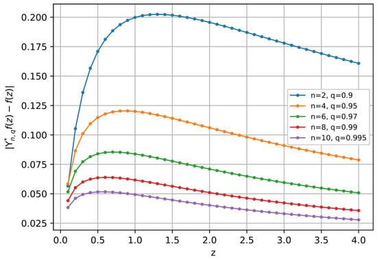
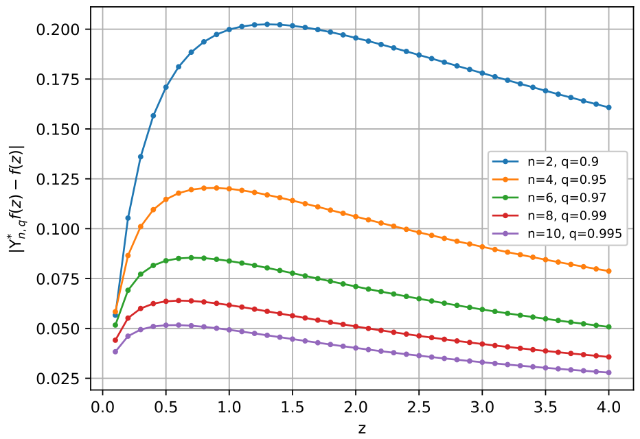
This section reports a fully specified reproducible computation of the pointwise error $|{\mathrm{Y}}_{n,q}^{*}f\left(z\right)-f\left(z\right)|$, addressing each of the gaps identified in this review, and the algorithm is given for each figure and table. The efficient numerical implementation of such structured operators is not only valuable for verifying theoretical estimates but is also crucial for their application in solving practical problems, such as the numerical treatment of fractional differential systems [34].

• Implementation details:

All computations reported below use the uniform kernel $\mathsf{\Psi }\left(y\right)=1$ for $y\in [0,1]$ and $\mathsf{\Psi }\left(y\right)=0$ elsewhere; the simple example of a kernel satisfying (a)–(c) was already given in Remark 1. This fixes $\alpha =1$ and $m_1={\int }_0^{1}ydy=\frac{1}{2}$. With this choice, step (3) of the Algorithm below reduces to the plain (non-q) integral ${\int }_0^{1}f\left(\frac{y-m_1+{\left[b\right]}_q}{{\left[n\right]}_q{q}^{b-1}}\right)dy$, which is evaluated by composite Simpson’s rule on $[0,1]$ with 200 equal subintervals (201 nodes); this was checked, for the $(n,q)$ pairs of Table 1, to agree with an adaptive-quadrature reference (MATLAB R2026a’s integral, default tolerances) to within ${10}^{-10}$. The truncation criterion in step (4) is sum over $b=0,1,2,\dots$ and stop at the first index B for which ten consecutive terms ${\upsilon }_n^q\left(z\right)\times \left(\mathrm{step}3\right)$ all fall below ${10}^{-14}$ in absolute value; in practice, $B\le 60$ for every $(n,q,z)$ combination used in Figure 1 and Table 1 and Table 2, consistent with the geometric decay of ${\upsilon }_n^q\left(z\right)$ established in the remark on convergence of the defining series in Section 2. These are the settings used to produce Figure 1 and Table 1, and are sufficient, together with the description below, to reproduce both independently.

Table 1. The $(n, q)$ pairs used in Figure 1, with the pointwise error $|{\mathrm{Y}}_{n,q}^{*}f\left(z\right)-f\left(z\right)|$ at $z=1$ and $z=2$, computed as described in the text.

Index	n	q	Error at $\mathit{z}=1$	Error at $\mathit{z}=2$
1	2	0.90	$1.998\times {10}^{-1}$	$1.956\times {10}^{-1}$
2	4	0.95	$1.200\times {10}^{-1}$	$1.061\times {10}^{-1}$
3	6	0.97	$8.381\times {10}^{-2}$	$7.102\times {10}^{-2}$
4	8	0.99	$6.170\times {10}^{-2}$	$5.101\times {10}^{-2}$
5	10	0.995	$4.931\times {10}^{-2}$	$4.023\times {10}^{-2}$

Figure 1. Pointwise error $|{\mathrm{Y}}_{n,q}^{*}f\left(z\right)-f\left(z\right)|$ for $f\left(z\right)=z/(1+z)$ over $z\in [0.1,4]$, computed by direct evaluation of (7) as described in the text, for the five $(n,q)$ pairs of Table 1. The error decreases monotonically in n across the whole plotted range.

Table 2. The King-type second central moment ${\delta }_n^q=\left({\mathrm{Y}}_{n,q}^{*}{(y-z)}^2\right)\left(z\right)$ against the classical/scaling-kernel moment ${\mathsf{\Gamma }}_{n,q}({(t-z)}^2,z)=\frac{z}{{\left[n\right]}_q}(1+\frac{z}{q})$ of Proposition 1, at $z=2$, for the $(n, q)$ pairs of Table 1: the inequality of Proposition 1 holds numerically in every case, confirming it is not asymptotically vacuous.

n	q	${\mathit{\delta }}_{\mathit{n}}^{\mathit{q}}=2\mathit{z}(\mathit{z}-{\mathit{r}}_{\mathit{n}}^{\mathit{q}}\left(\mathit{z}\right))$ at $\mathit{z}=2$	${\mathbf{\Gamma }}_{\mathit{n},\mathit{q}}({(\mathit{t}-\mathit{z})}^2,\mathit{z})$ at $\mathit{z}=2$
2	0.90	$2.275$	$3.392$
4	0.95	$1.347$	$1.674$
6	0.97	$0.948$	$1.100$
8	0.99	$0.702$	$0.782$
10	0.995	$0.565$	$0.616$

• Algorithm.

For each pair $(n,q)$ and each evaluation point z, (1) compute $r_n^q\left(z\right)$ from (6); (2) for $b=0,1,\dots$, compute the q-binomial coefficient ${\left({\displaystyle \genfrac{}{}{0pt}{}{n+b-1}{b}}\right)}_q$ from its product formula, the q-Pochhammer symbol ${(1+r_n^q\left(z\right))}_q^{n+b}={\prod }_{s=0}^{n+b-1}(1+q^s{r}_n^q\left(z\right))$, and hence the weight ${\upsilon }_n^q\left(z\right)$; (3) evaluate the Simpson-quadrature approximation of ${\int }_0^{1}f\left(\frac{y-m_1+{\left[b\right]}_q}{{\left[n\right]}_q{q}^{b-1}}\right)\mathsf{\Psi }\left(y\right)dy$; (4) accumulate ${\upsilon }_n^q\left(z\right)\times \left(\mathrm{step}3\right)$ over b until the truncation criterion is met; and (5) subtract $f\left(z\right)$ and take the absolute value. This is a direct elementary evaluation of (7) with no reliance on the closed forms derived in Section 3 and Section 4; so, it also serves as an independent numerical check on Theorem 1 and Corollary 1: at $z=0,1,2,3$, the computed values of $\left({\mathrm{Y}}_{n,q}^{*}{e}_1\right)\left(z\right)$ and $\left({\mathrm{Y}}_{n,q}^{*}{e}_2\right)\left(z\right)$ obtained this way agree with $r_n^q\left(z\right)$ and $z^2$, respectively, to within ${10}^{-10}$, for every $(n,q)$ pair in Table 1.

We illustrate the pointwise approximation error $|{\mathrm{Y}}_{n,q}^{*}f\left(z\right)-f\left(z\right)|$ over $z\in [0.1,4]$. In this notation, n stands for the degree (size) of the operator, while $q\in (0,1)$ acts as a tuning parameter governing the smoothing, with a lower curve reflecting a better approximation. The $(n,q)$ pairs behind each curve are listed in Table 1.

This illustration deliberately uses a single test function, $f\left(z\right)=z/(1+z)$: it is bounded, strictly increasing, and neither a polynomial nor asymptotically linear; so, none of the moment identities of Theorem 1 trivializes the resulting computation. It is worth stressing that the rate-of-convergence bounds of Section 4 are already proved uniformly over entire function classes ($C_B[0,\infty )$, $Li{p}_{\lambda }\left(\mu \right)$, and $R_{\nu ,\mathcal{D}}$, respectively), not for this function alone. The numerical experiment therefore corroborates, on one concrete instance, bounds that are already established analytically for every admissible h, rather than substituting for that analysis. What the present study can, and does, add is a second, exactly computable numerical comparison that complements Table 2; rather than varying n at fixed q, Table 3 varies q at fixed n, using the closed-form expressions of Equation (9) and Proposition 1 directly, with no quadrature or truncation involved.

Table 3. Dependence on q, for fixed operator degree $n=6$ and evaluation point $z=2$, of the King-type central moment ${\delta }_n^q$ and of the scaling-kernel moment ${\mathsf{\Gamma }}_{n,q}({(t-z)}^2,z)$, both evaluated exactly from their closed forms (9) and Proposition 1, respectively; no quadrature or truncation is involved.

q	${\mathit{\delta }}_{\mathit{n}}^{\mathit{q}}$ (King)	${\mathbf{\Gamma }}_{\mathit{n},\mathit{q}}({(\mathit{t}-\mathit{z})}^2,\mathit{z})$
0.80	$1.4791$	$1.8974$
0.85	$1.3035$	$1.6150$
0.90	$1.1442$	$1.3754$
0.93	$1.0565$	$1.2495$
0.95	$1.0011$	$1.1722$
0.97	$0.9483$	$1.0999$
0.99	$0.8979$	$1.0322$
0.995	$0.8857$	$1.0160$

5. Conclusions

We have introduced a King-type re-parametrization of the wavelet-assisted Kantorovich q-Baskakov operators, designed to reproduce the quadratic test function $e_2$ exactly. This exact reproduction is not merely formal: Proposition 1 proves, in closed form, that the resulting central moment ${\delta }_n^{q_n}$ is strictly smaller than the corresponding moment for the classical and scaling-kernel operators from which ${\mathrm{Y}}_{n,q_n}^{*}$ is built, for every $z>0$, $n\ge 1$, and $0<q\le 1$, confirmed numerically in Table 2 across n and Table 3 across q. Since this moment drives every rate-of-convergence estimate in Section 4, the improvement carries through to the modulus-of-smoothness, Lipschitz-type, and statistical convergence rates alike. These analytical results hold uniformly over the stated function classes; the numerical illustration (Figure 1, Table 1) corroborates them on one representative test function rather than establishing them independently. The construction draws on the Jackson q-calculus throughout and on a wavelet-theoretic scaling-kernel idea in its definition, but it makes no claim regarding quantum computing or a full multiresolution decomposition; a systematic multi-function numerical benchmark and a direct comparison with other published King-type or wavelet-Kantorovich constructions remain natural directions for future work.

References

- King, J.P. Positive linear operators which preserve x2. Acta Math. Hung. 2003, 99, 203–208. [Google Scholar] [CrossRef] [Scilit]
- Bernstein, S. Démonstration du théorème de Weierstrass fondée sur le calcul des probabilités. Commun. Soc. Math. Kharkow 1912, 13, 1–2. [Google Scholar]
- Aral, A.; Gupta, V. Generalized q-Baskakov operators. Adv. Oper. Theory 2011, 61, 619–634. [Google Scholar] [CrossRef] [Scilit]
- Lupaş, A. A q-analogue of Bernstein operator. Semin. Numer. Stat. Calc. 1987, 9, 85–92. [Google Scholar]
- Altomare, F.; Campiti, M. Korovkin-Type Approximation Theory and Its Applications; Walter de Gruyter Studies in Mathematics 17; de Gruyter: Berlin, Germany, 1994. [Google Scholar]
- Doğru, O.; Örkcü, M. King type modification of Meyer-König and Zeller operators based on the q-integers. Math. Comput. Model. 2009, 50, 1245–1251. [Google Scholar] [CrossRef] [Scilit]
- Yilmaz, Ö.G.; Gupta, V.; Aral, A. On Baskakov operators preserving the exponential function. J. Numer. Anal. Approx. Theory 2017, 46, 150–161. [Google Scholar] [CrossRef] [Scilit]
- Mursaleen, M.; Naaz, A.; Khan, A. Dunkl generalization of q-Szász-Mirakjan Kantorovich operators which preserve some test functions. J. Inequal. Appl. 2016, 2016, 1–18. [Google Scholar] [CrossRef] [Scilit]
- Mursaleen, M.; Naaz, A.; Khan, A. Improved approximation and error estimations by King type (p, q)-Szász-Mirakjan Kantorovich operators. Appl. Math. Comput. 2019, 348, 175–185. [Google Scholar] [CrossRef] [Scilit]
- Rao, N.; Shahzad, M.; Jha, N.K. Study of two dimensional α-modified Bernstein bi-variate operators. FILOMAT 2025, 39, 1509–1522. [Google Scholar] [CrossRef] [Scilit]
- Alamer, A.; Nasiruzzaman, M. Approximation by Stancu variant of λ-Bernstein shifted knots operators associated by Bézier basis function. J. King Saud Univ. Sci. 2024, 36, 103333. [Google Scholar] [CrossRef] [Scilit]
- Burban, I. Two-Parameter Deformation of the Oscillator Algebra and (p, q)-Analog of Two-Dimensional Conformal Field Theory. J. Nonlinear Math. Phys. 1995, 2, 384–391. [Google Scholar] [CrossRef] [Scilit]
- Mohiuddine, S.A.; Özger, Z.Ö.; Özger, F.; Alotaibi, A.M. Construction of a new family of modified Bernstein-Schurer operators of different order for better approximation. J. Nonlinear Convex Anal. 2024, 25, 2059–2082. [Google Scholar]
- Mursaleen, M.; Ansari, K.J.; Khan, A. On (p, q)-analogue of Bernstein operators. Appl. Math. Comput. 2015, 266, 874–882, Erratum in Appl. Math. Comput. 2016, 278, 70–71. [Google Scholar] [CrossRef] [Scilit]
- Özger, F.; Aslan, R.; Ersoy, M. Some Approximation Results on a Class of Szász-Mirakjan-Kantorovich Operators Including Non-negative parameter α. Numer. Funct. Anal. Optim. 2025, 46, 481–484. [Google Scholar] [CrossRef] [Scilit]
- He, Z.; Zhong, H.; Shi, X.; Zhao, C.; Wen, J.; Shang, M. Accelerating the tuning process for optimizing DNN operators by ROFT model. Sci. Rep. 2025, 15, 36327. [Google Scholar] [CrossRef] [Scilit]
- Li, M.; Li, L.; Zhang, Z.; Zhang, Q. A novel method for generating permutation mass functions using permutations to represent class bias. Expert Syst. Appl. 2026, 319, 132004. [Google Scholar] [CrossRef] [Scilit]
- Ayman-Mursaleen, M. Quadratic function preserving wavelet type Baskakov operators for enhanced function approximation. Comp. Appl. Math. 2025, 44, 395. [Google Scholar] [CrossRef] [Scilit]
- Kumar, S.; Moreka, A.E.; Mursaleen, M. On wavelets Kantorovich (p, q)-Baskakov operators and approximation properties. J. Ineq. Appl. 2023, 2023, 134. [Google Scholar] [CrossRef] [Scilit]
- Kumar, S.; Moreka, A.E.; Mursaleen, M. Statistical approximation using wavelets Kantorovich (p, q)-Baskakov operators. Analysis 2024, 44, 105–114. [Google Scholar] [CrossRef] [Scilit]
- Nasiruzzaman, M. Function preserving the wavelets-associated approximation by Szasz-type operators in quantum calculus. J. Inequal. Appl. 2025, 2025, 157. [Google Scholar] [CrossRef] [Scilit]
- Nasiruzzaman, M.; Alqahtani, R.T.; Mohiuddine, S.A. Approximation Properties of a New Class of Beta-Type Szasz–Mirakjan Operators. J. Math. 2025, 2025, 6680828. [Google Scholar] [CrossRef] [Scilit]
- Nasiruzzaman, M.; Kiliçman, A.; Ayman-Mursaleen, M. Construction of q-Baskakov operators by wavelets and approximation properties. Iran. J. Sci. Technol. Trans. A Sci. 2022, 46, 1495–1503. [Google Scholar] [CrossRef] [Scilit]
- Savaş, E.; Mursaleen, M. Bézier type Kantorovich q-Baskakov operators via wavelets and some approximation properties. Bull. Iran. Math. Soc. 2023, 49, 68. [Google Scholar] [CrossRef] [Scilit]
- Nasiruzzaman, M.; Alotaibi, A. Kantorovich extension of parametric generalized q-Schurer operators and their approximation properties. Mathematics 2025, 13, 3770. [Google Scholar] [CrossRef] [Scilit]
- Daubechies, I. Ten Lectures on Wavelets; SIAM: Philadelphia, PA, USA, 1992. [Google Scholar]
- Graps, A. An introduction to wavelets. IEEE Comput. Sci. Eng. 1995, 2, 50–61. [Google Scholar] [CrossRef] [Scilit]
- Meyer, Y. Wavelets and Operators; Cambridge University Press: Cambridge, UK, 1992; Volume 1. [Google Scholar]
- Ayman-Mursaleen, M.; Nasiruzzaman, M.; Sharma, S.K.; Cai, Q.-B. Invariant means and lacunary sequence spaces of order (α, β). Demonstr. Math. 2024, 57, 20240003. [Google Scholar] [CrossRef] [Scilit]
- Gadjiev, A.D. The convergence problem for a sequence of positive linear operators on unbounded sets, and theorems analogous to that of P.P. Korovkin. Sov. Math. Dokl. 1974, 15, 1433–1436. [Google Scholar]
- Aral, A.; Doğru, O. Bleimann, Butzer, and Hahn operators based on the q-integers. J. Inequal. Appl. 2007, 1–12. [Google Scholar]
- Aral, A.; Doğru, O. Bernstein-Baskakov-Kantorovich operators and Lipschitz-type maximal functions. Colloq. Math. Soc. Janos Bolyai. 1990, 58, 469–496. [Google Scholar]
- Savaş, R.; Patterson, R.F. Multidimensional sliding window Pringsheim convergence for measurable functions. Rend. Circ. Mat. Palermo 2024, 73, 689–698. [Google Scholar] [CrossRef] [Scilit]
- Alqhtani, M.; Sadek, L.; Hammouch, Z.; Saad, K.M. Efficient numerical schemes for linear fractional differential systems with applications to diffusion problems. J. Frankl. Inst. 2025, 362, 108144. [Google Scholar] [CrossRef] [Scilit]
Disclaimer/Publisher’s Note: The statements, opinions and data contained in all publications are solely those of the individual author(s) and contributor(s) and not of MDPI and/or the editor(s). MDPI and/or the editor(s) disclaim responsibility for any injury to people or property resulting from any ideas, methods, instructions or products referred to in the content. |
© 2026 by the authors. Licensee MDPI, Basel, Switzerland. This article is an open access article distributed under the terms and conditions of the Creative Commons Attribution (CC BY) license.