


Abstract
Medical image reconstruction began with an exact mathematical result. In 1917, Radon showed how to recover a function from its line integrals, providing the mathematical basis for computed tomography, positron emission tomography, and single-photon emission computed tomography. This review follows the development of reconstruction from analytical inversion to modern deep learning. We first present the Radon transform, its attenuated and three-dimensional generalizations, and the corresponding inversion formulae, including filtered backprojection. We then review iterative and optimization-based methods, including maximum-likelihood expectation-maximization, variational regularization, and compressed sensing. The discussion proceeds to deep learning, covering convolutional and transformer architectures, algorithm unrolling, physics-informed networks, neural operators, and generative diffusion priors. Our central argument is that analytical, iterative, and learned reconstruction are different formulations of the same inverse problem rather than competing paradigms. Many learned components derive from classical formulations, and many classical operators admit learnable counterparts. We conclude by discussing open challenges related to theoretical guarantees, trustworthiness, data efficiency, federated learning, and regulatory validation. The most reliable learned systems are likely to retain the mathematical and physical structure of established reconstruction methods.
Keywords:
Radon transform; tomography; CT; PET; SPECT; image reconstruction; deep learning; inverse problems MSC:
44A12; 65R10; 92C55; 68T07
1. Introduction
Medical imaging is among the most significant achievements of applied mathematics, physics, and engineering in the twentieth century. The non-invasive visualization of the interior of the human body is made possible through the solution of complex inverse problems. This enables physicians to locate tumors and internal organs, monitor the response of tumors to treatment, map blood flow, quantify metabolic activity, and guide surgery. Whether involving X-rays, gamma rays, or radiofrequency pulses interacting with tissue, each imaging modality generates projection or frequency-domain measurements from which an image must be reconstructed. The accuracy, stability, and computational cost of this reconstruction determine the diagnostic utility of the resulting image.
At the heart of computerized tomography (CT), positron emission tomography (PET), and single-photon emission computed tomography (SPECT) lies the celebrated Radon transform, which, in the two-dimensional case, maps a so-called “point function” (Punktfunktion), , where denotes an arbitrary point in the plane, to a “line function” (Geradenfunktion), following Radon’s original terminology [1,2]. A line function is simply a function defined on the set of straight lines. In modern notation, this line function is written as
where G is an arbitrary straight line in the plane. The mathematical challenge of inverting the integral transform defined in Equation (1) involves recovering, or reconstructing, f from its projections. It was solved analytically by Johann Radon in 1917 [1]. Radon followed unpublished work by Hendrik Antoon Lorentz from 1905, in which the original problem was formulated, and a three-dimensional function was recovered from its integrals over corresponding planes [3]. The inversion of the three-dimensional transform was later presented by Hermann Bockwinkel in his study of light propagation in biaxial crystals, where the inversion formula was explicitly attributed to Lorentz [4,5].
Little could Radon have anticipated that this abstract mathematical construction would eventually become one of the foundations of modern medical imaging. He died in 1956, before the invention of X-ray CT transformed his theory into clinical reality. Decades later, Cormack established the mathematical foundations of modern X-ray tomography [6,7], while Hounsfield developed the first practical X-ray CT scanner [8], initially unaware that both Radon and Cormack had already demonstrated, at least theoretically, that images could be reconstructed from projection data [9]. Their contributions were recognized with the 1979 Nobel Prize in Physiology or Medicine. These foundational developments paved the way for practical analytical reconstruction algorithms. Derived from the Fourier slice theorem [10], filtered backprojection (FBP) became the classical reconstruction algorithm in CT and emission tomography [11,12,13].
Over the following decades, a series of important advances emerged in image reconstruction, including the maximum-likelihood expectation-maximization (MLEM) algorithm [14] and its ordered-subset expectation-maximization acceleration (OSEM) [15], which provided a principled statistical framework for modeling of photon-counting noise. Furthermore, the theory of compressed sensing [16,17] demonstrated that sparse images can be reconstructed accurately from highly undersampled measurements, beyond what would be predicted by the Shannon–Nyquist sampling theorem [18,19]. In parallel, iterative regularization methods, particularly total variation (TV) minimization [20], emerged as powerful tools for suppressing reconstruction artifacts while preserving important image features such as edges. Analytical approaches to image reconstruction also continued to evolve, including the Tretiak–Metz reconstruction approach for emission tomography [21], advances in the inversion of the attenuated Radon transform [22,23], and reconstruction methods based on piecewise-continuous polynomial approximations for PET and SPECT [24,25,26,27]. Such algorithms have also been implemented within STIR (Software for Tomographic Image Reconstruction) [28].
More recently, deep learning has become an important paradigm in medical imaging and image analysis [29,30]. The U-Net architecture [31] demonstrated the effectiveness of convolutional encoder–decoder networks with skip connections for biomedical image segmentation. Since then, deep learning methods have been applied to a wide range of tasks in medical image analysis [32], namely: image reconstruction [33,34], segmentation [35], registration [36], super-resolution [37], and multi-modal fusion [38]. The introduction of transformer architectures [39] and vision transformers [40] has further expanded available methods, thus enabling the modeling of long-range spatial dependencies that complement the local feature extraction of convolutional networks. Hybrid approaches have sought to connect analytical reconstruction theory with deep learning [41,42,43]; however, such efforts remain relatively limited.
Despite this progress, a significant gap persists in the literature. Analytical and deep learning approaches have largely evolved independently, with limited integration of ideas and methodologies. As a result, the relationship between analytical and modern learning-based methodologies remains insufficiently explored. In this review, we argue that these approaches are more closely related than is often acknowledged. Both emerge from the same underlying mathematical foundations, including inverse problems, functional and complex analysis, approximation theory, and optimization. Figure 1 summarizes the principal milestones discussed in this review along a single timeline spanning the analytical, iterative, and deep-learning eras.
Figure 1.
A century of medical imaging mathematics. Selected milestones from the Radon transform (1917) to contemporary foundation models, partitioned into an analytical era, an iterative/sparse era, and a deep-learning era.
Several comprehensive surveys cover parts of this landscape. Deep learning for tomographic reconstruction is reviewed by Wang et al. [44], deep learning for inverse problems in imaging by Ongie et al. [45], and artificial intelligence for PET reconstruction by Reader and Pan [46]. These surveys are organized by application domain or by architecture, and none develop the operator-level correspondence between classical and learned reconstruction pursued here. Classical analytical and iterative methods are treated thoroughly in standard texts [10,47]. The present review differs in three respects. First, it treats analytical, iterative, and learned reconstruction within a single mathematical framework. Learned methods often derive from classical formulations, and the correspondences between classical and learned operators are synthesized explicitly in tabular form later in the manuscript. Second, it covers the emission-tomography thread, including the attenuated Radon transform and its analytic inversion, which falls outside the scope of the CT- and magnetic-resonance-imaging (MRI) focused surveys above. Third, it closes with a concrete research direction arising from this viewpoint: the embedding of analytical inversion operators beyond FBP into learned architectures.
This is a narrative review, organized by mathematical structure rather than by a systematic search protocol. The literature was selected to trace the development of reconstruction methodology across the analytical, iterative, and learned paradigms, from Radon’s inversion formula of 1917 to work published in 2026. Foundational works were included for the analytical and iterative eras, while deep-learning methods were included if they introduced a major class of approaches or made an explicit connection to classical reconstruction. Emphasis is placed on tomographic modalities, namely CT, PET, and SPECT, with methods from other modalities included where they introduced techniques subsequently adopted in tomography. Within the learned paradigm, post-processing, unrolled, physics-informed, operator-learning, and generative methods are each represented for CT, and the emission-tomography counterparts are included where such methods have been reported. Where a class of methods has been developed only for CT or MRI, this is stated. The literature is synthesized comparatively rather than as a sequence of individual studies. The comparison of paradigms and the correspondence between classical and learned methods are summarized in tabular form in Section 6, and Table 1 places the principal milestones on a common timeline.
Table 1.
Chronological milestones in mathematical and computational methods for medical image reconstruction.
2. Mathematical Foundations: The Radon Transform and Its Generalizations
This section introduces the mathematical foundations underlying tomographic imaging. We begin with the classical two-dimensional Radon transform, before discussing important generalizations, including the attenuated and three-dimensional Radon transforms.
2.1. The Classical Radon Transform
Let be a compactly supported function. The two-dimensional Radon transform maps f to its line integrals over sets of parallel lines in the plane [57]. More generally, the Radon transform in associates a function with its integrals over hyperplanes [10].
The line integral of a continuous function along a differentiable curve is defined by:
where is a bijective map, namely the parameterization of the curve C, and denotes the Euclidean norm in . In tomographic imaging, the curves of interest are straight lines. The Radon transform is obtained by restricting the above construction to straight lines. To parameterize families of parallel lines, we adopt the following coordinate system.
A line L on the -plane can be uniquely specified by the signed distance from the origin, with , and the angle with the -axis, with , see Figure 2. If we denote the corresponding unit vectors parallel and perpendicular to L by and , respectively:
then every point on L in Cartesian coordinates can be expressed in terms of the line coordinates () via
where denotes the arc length, namely,
Equations (4) yield the parameterization
where represents the arc length along L. It is straightforward to deduce that , thus Equation (5) is a natural parameterization of the line L. For a straight line L parameterized by its arc length , Equation (2) reduces to
Solving Equations (4) for yields:
Figure 2.
Radon transform: A two-dimensional function, , and its corresponding projections, , in Cartesian and local coordinates.
We denote the space of rapidly decreasing (or Schwartz) functions on by , namely:
where
Then, the two-dimensional Radon transform of f, , denoted by g, is defined as
Here, f is introduced as compactly supported, which suffices for the line integral in Equation (2) to be well defined. From Equation (10) onward, we work in the Schwartz class , which guarantees the rapid decay required by the Fourier slice theorem, the inversion formula, and the range conditions. The resulting function is referred to as the sinogram, the measured data in CT and emission tomography. Using Dirac’s delta function (line impulse), the Radon transform may be written as [25]:
The Fourier slice theorem provides the mathematical foundation of analytical tomographic reconstruction [13]. It establishes a direct relationship between the Radon transform and the Fourier transform [58] and may be expressed as follows:
where is defined by
is defined by
is defined in Equation (10), where the variables are related through
Thus, the one-dimensional Fourier transform of a projection coincides with the restriction of the two-dimensional Fourier transform of the image to the corresponding radial line in frequency space [10]. This relationship forms the basis of FBP, enabling the reconstruction of an image from its projections (sinogram).
The mathematical analysis of tomographic reconstruction is closely linked to the properties of the Radon transform. Questions of uniqueness, stability, and invertibility are central to understanding the effects of noise, incomplete data, and reconstruction artifacts [59]. Explicit singular value decompositions of the Radon transform provide valuable insight into the structure of the inverse problem and the role of filtering in analytical reconstruction [60]. In many imaging modalities, however, the measured data are affected by additional physical phenomena, requiring extensions of the classical Radon transform.
2.2. The Attenuated Radon Transform
In SPECT, gamma rays emitted by a radiolabeled tracer are attenuated as they propagate through tissue before reaching the detector. Consequently, the measured data are described not by the classical Radon transform but by the attenuated Radon transform. Unlike SPECT, in PET, two annihilation photons are emitted in approximately opposite directions and detected in coincidence, defining a “line of response.” Since the photons traverse complementary segments of this line, their combined attenuation is independent of the annihilation position and appears as a multiplicative factor of the Radon transform. If denotes the spatially varying attenuation map, the attenuated Radon transform is defined by
The exponential factor in Equation (16) accounts for the attenuation accumulated along the photon path between the emission point and the detector. Unlike the classical Radon transform, the attenuation map enters explicitly into the forward model, making the corresponding inverse problem substantially more challenging. The development of explicit inversion formulae for the attenuated Radon transform [22,23,61,62] established the mathematical foundation for quantitative SPECT reconstruction.
2.3. The Three-Dimensional Radon Transform and PET
In three space dimensions, the Radon transform integrates over planes rather than lines. The three-dimensional Radon transform of f, , denoted by g, is defined as
where represents parallel planes, denotes an area differential, and is defined in Equation (8) for . Each plane is uniquely characterized by a vector and a scalar, namely, its unit normal vector ,
and its signed distance from the origin . The equation of the plane is
Furthermore, we suppose that intersects the -plane in an angle , and the -plane in an angle (spherical angles). This implies that we can rewrite the normal vector in spherical angles as follows:
Inserting Equation (20) in Equation (19) yields
According to Equation (21), an alternative way to express the three-dimensional Radon transform of a function involves a Dirac delta, or a “plane impulse”, namely
PET scanners operating in three-dimensional mode measure coincidence events along lines of response connecting pairs of detectors, so the measured data are samples of the three-dimensional X-ray transform, not of the plane-integral Radon transform. The three-dimensional Radon transform enters as an intermediate representation. Plane integrals can be formed from line-integral data by integrating the X-ray transform over a family of parallel lines that foliate each plane. This operation requires adequate sampling of those lines and is therefore restricted by the finite axial acceptance of the scanner, an assumption underlying rebinning schemes that pass through plane-integral data [63]. The spline-based inversion of the three-dimensional Radon transform [64] applies to plane-integral data obtained in this way and thus provides an analytically explicit route from three-dimensional PET data to the image through the intermediate Radon representation, rather than a direct inversion of the measured line integrals.
3. Analytical Reconstruction
The starting point of analytical reconstruction is the inversion formula derived by Radon in his seminal 1917 paper [1]. Radon parameterized straight lines by their normal angle , rather than the angle adopted throughout this review. He considered the mean value of the line-function data over all tangent lines to the circle centered at the reconstruction point P with radius q, denoted by , namely,
where g denotes the Radon transform defined in Equation (10). The parameterizations are related by
since Radon measured the angle of the line normal, whereas throughout this review, is defined according to the convention introduced in Equation (7) and Figure 2. Using the parameterization introduced in Section 2, Equation (23) becomes
where is defined in the first of Equations (7). Radon then obtained an explicit inversion formula for the transform defined in Equation (1), which would later become known as the Radon transform:
where the integral is understood in the Stieltjes sense. Equivalently,
The key idea of Radon’s derivation was to relate the averaged line-function data to the circular means of the unknown function, thereby reducing the reconstruction problem to an Abel integral equation. To simplify the analysis, Radon first considered the special case in which the reconstruction point coincides with the origin. In this case, the averaged projection data satisfy
where denotes the circular mean of f over the circle of radius r centered at the origin. Introducing the change of variables
reduces this relation to the classical Abel integral equation [65,66], whose explicit inversion recovers the circular means of the unknown function. Substituting these into the averaged line-function formula yields Radon’s inversion Formula (26).
3.1. Filtered Backprojection
Although Radon’s original derivation proceeded through Abel inversion, later analyses established an equivalent formulation of the inverse Radon transform in terms of the Hilbert transform (). The Hilbert transform of a function is defined by the Cauchy principal value integral
In this formulation, the reconstruction is expressed in terms of the derivative of the Hilbert transform of the sinogram. The Fourier transform of the Hilbert transform is given by [58]
where H denotes the Hilbert transform. Since
applying the Fourier differentiation property then yields
Thus, the operator corresponds to multiplication by the so-called ramp filter, , in the Fourier domain. The Fourier Slice Theorem identifies the one-dimensional Fourier transform of each projection with the corresponding radial slice of the two-dimensional Fourier transform of the image. Combined with the ramp-filter representation above, the reconstruction problem reduces to filtering each projection and subsequently backprojecting the filtered projections over all projection angles. This procedure constitutes the classical FBP method, which has remained the predominant analytical reconstruction algorithm in clinical CT for several decades and is also widely used in PET and SPECT because of its computational efficiency [10,47,58].
The FBP reconstruction of a two-dimensional function f from its projections g is given by
where is defined in the first of Equations (7), ∗ denotes convolution with respect to the detector variable , and Q denotes the reconstruction kernel, whose one-dimensional Fourier transform is given by
where Q is understood as a tempered distribution, and the convolution in Equation (33) is interpreted accordingly. In practice, the ideal ramp filter is commonly multiplied by a low-pass apodization window, such as the Hann, Hamming, Butterworth, or Shepp-Logan window, thereby providing a trade-off between noise suppression and spatial resolution [10,47]. Among these, the Shepp-Logan filter is one of the most widely used choices in clinical practice.
The integration over in Equation (33) is the backprojection operator, namely the adjoint of the Radon transform. It is defined by the identity with respect to the inner products on image and sinogram space. Backprojection assigns each projection value to all points on the corresponding line and integrates over all angles. The adjoint alone does not invert the transform, since is a smoothing operator rather than the identity. The ramp filter provides the correction required for inversion.
Despite its computational efficiency and widespread clinical adoption, FBP assumes an ideal line-integral acquisition model and therefore cannot explicitly account for physical effects such as detector response, photon attenuation, scatter, or Poisson counting statistics. Moreover, its sensitivity to measurement noise and angular undersampling often leads to high-frequency noise amplification and streak artifacts. These limitations have motivated the development of the iterative reconstruction methods discussed in Section 4, and more recently, deep learning-based approaches presented in Section 5.
3.2. Spline-Based Reconstruction
Spline-based methods represent the image or projection data by smooth piecewise-polynomial functions rather than piecewise-constant pixels. They extend earlier work on reconstruction from projections [67,68] and on spline discretizations of the Radon transform [69,70]. Further developments include box-spline formulations of Radon projection [71,72] and optimized spline and Kaiser-Bessel projectors for few-view CT [73,74].
The spline reconstruction technique (SRT) employs splines not to discretize the forward projector, but to evaluate the inverse Radon transform. The inverse can be written in terms of the Hilbert transform as
The essential operation is the derivative with respect to of the Hilbert transform of the sinogram. In SRT, the sinogram is approximated at each angle by cubic splines in the detector variable , and this operation is then carried out analytically on the spline representation rather than by numerical differentiation of noisy data [25]. Spline approximation thus enters the inversion formula itself, rather than serving only as an interpolation step. It should be stressed that this is not a different inversion formula. By Equation (32), the operator corresponds, up to a constant factor, to multiplication by in the Fourier domain, so Equation (35) and the FBP Formula (33) are equivalent representations of the same inversion identity. The differences between SRT and FBP arise entirely from where and how the continuous formula is approximated. FBP discretizes the ramp filter, applies it to the sampled sinogram, typically in the frequency domain, and controls the resulting amplification of high-frequency noise using an apodization window chosen by the user. SRT instead replaces the sampled sinogram by a cubic spline in and evaluates on the spline in closed form, so that the derivative acts on a smooth interpolant rather than directly on the noisy samples, and no explicit apodization window is required. The two methods therefore differ in their noise behavior, treatment of detector sampling, and computational structure, not in the underlying inversion identity. This distinguishes SRT from FBP, where reconstruction is performed by ramp filtering followed by backprojection.
The attenuated spline reconstruction technique (aSRT) [27] applies the same idea to the inverse attenuated Radon transform of Novikov [22] and of Fokas et al. [62]. In this case, the relevant one-dimensional functions in the inversion formula are represented by splines. These include the Hilbert transforms of the attenuation map and of two sinusoidal functions of the attenuated sinogram. As a result, attenuation correction enters the formula directly, rather than as a post-processing step. The same piecewise-polynomial strategy extends to three dimensions, where the Radon transform integrates over planes [64].
3.3. Orthogonal Polynomial Reconstruction
Orthogonal polynomial methods provide another analytical route to Radon inversion. The object, or sometimes the projection data, is expanded in an orthogonal polynomial basis adapted to the geometry of the problem. Reconstruction, then, is reduced to recovering the expansion coefficients, rather than directly reconstructing pointwise image values. Writing gives, by linearity, , hence the unknowns are the coefficients , obtained by matching the measured sinogram against the known projected basis functions . This idea goes back to Cormack, who used circular harmonics and Zernike-type expansions to reconstruct a function from its line integrals [6,7]. The singular value decomposition of the Radon transform can be written in terms of orthogonal polynomial bases [60,75]. Louis later clarified how orthogonal expansions describe the null space of the transform [76]. Related reconstruction formulae based on multivariate orthogonal polynomials were subsequently developed as part of approximation theory [77,78]. Chebyshev decomposition combined with backprojection has also been used for fast reconstruction directly from sinogram data [79].
For Chebyshev polynomials of the first kind, the sinogram is expanded, for each angle , as
Substituting the Chebyshev expansion into the Hilbert transform term of Equation (35) allows that term to be evaluated analytically. In the weighted finite Hilbert-transform setting, each maps, up to normalization, to a Chebyshev polynomial of the second kind, so that the derivative required in the inversion formula is computed term by term. As in SRT, the approximation enters the inversion formula itself. The difference is that splines give a local representation, whereas Chebyshev polynomials give a global one. A Chebyshev-based scheme of this type was introduced for analytical PET reconstruction [80]. A practical issue is that standard Chebyshev interpolation uses non-uniform nodes, whereas tomographic detectors are almost always uniformly spaced. Interpolation on almost equally spaced points addresses this mismatch and reduces the Runge phenomenon [81].
3.4. Further Analytical Reconstruction Methods
The method of FBP, along with the spline and orthogonal polynomial methods discussed above, are not the only analytical inversion techniques for the Radon transform. The most direct alternative is Fourier inversion, which follows from the Fourier slice theorem, see Section 2. In this approach, the image is reconstructed by applying the inverse Fourier transform to the one-dimensional Fourier transforms of its projections. The FBP algorithm can be viewed as a particular implementation of this inversion, obtained by expressing the inverse Fourier transform as a filtering (convolution) step followed by backprojection [10,47].
A different approach is provided by moment methods. The projection moments
where is as defined in Equation (3), relate explicitly to the image moments, by the definition of the Radon transform. This yields a means of recovering the low-order structure of the object, or of building finite-dimensional approximations from moment data [82].
Furthermore, analytical inversion extends beyond the classical Radon transform. In SPECT, attenuation is part of the forward model, so the corresponding operator is the attenuated Radon transform. For this specific operator, explicit analytical reconstruction is provided both by the inversion formulae of Novikov [22] and Kunyansky [23], and by the unified-transform approach of Fokas [83]. Their advantage is that attenuation correction enters the inverse directly, rather than as a separate correction after reconstruction. Exact FBP-type formulae have also been derived for fan-beam [47], cone-beam [84,85], and helical [86] geometries, while the approximate but widely used Feldkamp algorithm handles circular cone-beam scans [49]. Together, these methods show that analytical reconstruction is not limited to standard parallel-beam FBP. It can also use the specific structure of the Radon transform, or of a related transform, instead of solving the inverse problem by general numerical optimization.
4. Iterative and Optimization-Based Reconstruction
As noted at the end of Section 3, FBP assumes an idealized acquisition model based on line-integrals, thus it cannot explicitly account for detector response, photon attenuation, scatter, or Poisson counting statistics. Iterative reconstruction methods address these limitations by explicitly modeling the physics and statistics of the acquisition process within an optimization process. However, this comes at the expense of substantially greater computational cost than FBP.
4.1. Algebraic and Statistical Iterative Methods
The earliest iterative approaches to tomographic reconstruction were purely algebraic. In this direction, the algebraic reconstruction technique (ART) [48] applies Kaczmarz’s classical row-action method for linear systems [87] to the discretized imaging equations, updating the current image estimate by sequentially projecting onto the hyperplane defined by each measured ray-sum. While historically important, ART does not account for the Poisson-distributed nature of photon-counting measurements in emission tomography, motivating a statistical reformulation of the reconstruction problem [88].
The transition to the discrete setting is obtained by expanding the image in a pixel or voxel basis, so that denotes the value associated with the j-th pixel or voxel. Sampling the sinogram along m rays and collecting the n image values into a vector turns the continuous model into the linear system . The matrix is the discrete counterpart of , and its entry represents the contribution of pixel j to measurement i. The transpose, , is the discrete counterpart of the adjoint . Thus, backprojection in the continuous setting corresponds to multiplication by in the discrete setting.
In PET and SPECT, the number of photons detected along each line of response is well modeled as a Poisson random variable whose mean is given by a linear forward model , where is the system matrix and denotes the probability that an emission from voxel j is detected in bin i. Maximizing the corresponding Poisson log-likelihood leads to the MLEM algorithm [14], with multiplicative update
where denotes the measured counts in bin i (the sampled entries of the sinogram g of Section 2) and the current estimate of voxel j at iteration n. In contrast to FBP, each MLEM iteration is guaranteed to increase the log-likelihood monotonically, and the algorithm preserves non-negativity of the image estimate automatically. This monotonicity is not specific to tomography. It follows from the structure of MLEM as an instance of the general expectation-maximization (EM) framework of Dempster, Laird, and Rubin [89], in which each iteration maximizes a lower bound on the observed-data log-likelihood that is tight at the current iterate. The statistical properties in the case of emission tomography, including the behavior of the maximum-likelihood estimator itself, were analyzed by Vardi, Shepp, and Kaufman [90], following the closely related EM formulation of Lange and Carson [91]. A well-known drawback is that MLEM converges relatively slowly and, without early stopping or regularization, the image estimate becomes increasingly noisy as iterations progress. This behavior motivated maximum a posteriori (MAP) formulations incorporating smoothness priors employed on the image, such as the Bayesian reconstruction [50] and the one-step-late algorithm [92], which modifies the EM update to accommodate a Gibbs prior.
The OSEM algorithm [15] accelerates MLEM. In particular, it partitions the projection data into disjoint subsets and accordingly updates the image estimate using one subset per sub-iteration rather than the full data set. This yields an order-of-magnitude reduction in the number of full iterations required for a given image quality. As a consequence, OSEM has become the iterative reconstruction method of choice in emission tomography, implemented on essentially all commercial PET and SPECT systems [93,94]. It is worth noting that the acceleration comes at a cost, since each sub-iteration uses only part of the data, and OSEM therefore does not converge to a fixed point in general, but cycles among several limit points, one per subset. In practice, it is terminated after a fixed number of iterations rather than run to convergence, which turns the iteration count itself into an implicit form of regularization. Convergent alternatives exist, namely the separable paraboloidal surrogates (SPS) family, which replaces the EM surrogate with a tighter quadratic surrogate admitting explicit penalized-likelihood maximization [52], and its relaxed ordered-subsets variant, which recovers subset-based acceleration without sacrificing that guarantee by introducing a diminishing relaxation parameter across iterations [95].
4.2. Variational and Regularization-Based Methods
The discrete forward operator A inherits the ill-posedness of the continuous transform it discretizes, whether the classical Radon transform, its attenuated counterpart, or the associated X-ray transform of Section 2. Its singular values decay rapidly toward zero, and A is consequently severely ill-conditioned. The least-squares solution, , is therefore unstable, since the noise components associated with the smallest singular values enter the solution amplified by the reciprocals of those values. Regularization restores stability by augmenting the data-fidelity term with a certain penalty, leading to the variational problem
where y denotes the discretized measurement data, that is, the sinogram g sampled on a finite set of rays, is a regularization functional incorporating prior assumptions about the image, and balances the two terms. Equation (39) is the generic form of the variational problem, with a quadratic data-fidelity term appropriate to additive Gaussian noise. For emission tomography, where the data follow the Poisson model of Section 4.1, the quadratic term is replaced by the negative Poisson log-likelihood, yielding the penalized-likelihood objective addressed by the surrogate algorithms discussed there [52]. The quadratic form remains relevant to emission tomography in the high-count limit, where the Poisson likelihood is well approximated by a weighted least-squares term, and as the form in which most of the algorithms in this section are stated. The classical choice is the quadratic Tikhonov functional [96,97], with L denoting a discrete gradient operator, for which (39) admits the closed-form normal equations
The penalty term limits the influence of the small singular values of A on the reconstruction, stabilizing it but, by penalizing gradient energy, oversmoothing edges [98].
Total variation (TV) regularization [20] instead sets , penalizing the -norm of the image gradient. Since TV penalizes gradient magnitude rather than gradient energy, it suppresses noise while preserving sharp edges [99]. The functional is convex, however non-smooth, so its minimizer is characterized not by a vanishing gradient but by the subdifferential optimality condition, namely
where ∂ denotes the subdifferential. This non-smoothness rules out direct gradient descent, and specialized first-order algorithms are therefore required. The iterative shrinkage-thresholding algorithm addresses the composite objective , with smooth and convex but non-smooth, by alternating a gradient step on F with a proximal step on G, namely:
where
where denotes the proximal mapping of Moreau [100], and the step size satisfies , since is a Lipschitz constant for . Its accelerated variant, the fast iterative shrinkage-thresholding algorithm (FISTA) [101], applies the same proximal step at an extrapolated point built from the two previous iterates, improving the rate of convergence of the objective from to . The alternating direction method of multipliers (ADMM) [102,103,104,105], the closely related split Bregman method [106,107], and first-order primal–dual methods such as the Chambolle–Pock algorithm [108] solve the associated saddle-point problem without requiring differentiability of the objective. In tomographic imaging specifically, TV-regularized reconstruction has been demonstrated for constrained cone-beam CT [109] and, combined directly with the expectation-maximization update of Section 4, for penalized reconstruction under Poisson statistics [110,111,112]. A further refinement penalizes the total variation of the sinogram in addition to that of the image, for which existence, uniqueness, and stability of the resulting variational problem have been established [113], illustrating how the variational and statistical iterative viewpoints combine in practice.
A well-known artifact of standard TV regularization is that, because the penalty favors piecewise-constant images by design, it can introduce a staircasing effect in regions that are genuinely smoothly varying [114]. Higher-order functionals address this by incorporating derivatives beyond the first into the penalty. Total generalized variation (TGV) [115] regularizes selectively across regularity levels, thereby avoiding staircasing while retaining edge preservation, and related models combine the total variation with the total variation of the first derivatives [116] or with infimal-convolution constructions [117,118]. In the same spirit, an augmented TV functional has recently been introduced for Radon-type inverse problems [119], where analysis of the resulting functional’s subdifferential yields reconstructions that suppress staircasing while preserving edges. These are members of a large family of TV-type functionals, surveyed by Burger and Osher [120].
4.3. Compressed Sensing and Sparse Recovery
Compressed sensing [16,17] established that signals admitting a sparse representation in a suitable basis can be recovered with high probability from far fewer linear measurements than predicted by the celebrated Shannon-Nyquist sampling principle [18,19]. Under appropriate conditions on the measurement operator, most commonly, the restricted isometry property (RIP) [121], this recovery is guaranteed. A matrix A satisfies the RIP of order s with constant if
for every s-sparse vector f. Thus, A approximately preserves the Euclidean norm of all sparse vectors. If is sufficiently small, then the relaxation recovers the same solution as the combinatorial sparsest-solution problem. In tomographic reconstruction, this theory motivates image recovery from angularly undersampled, or otherwise incomplete, projection data. A standard constrained formulation is the following:
where is a sparsifying transform [51] and is an upper bound on the expected measurement noise. By Lagrangian duality, Equation (45) is equivalent, for a suitable multiplier , to the unconstrained problem
which has the same composite form as the variational problem (39), and is solved by the same first-order algorithms. Setting recovers TV regularization. In this case, sparsity is imposed on the image gradient rather than on the image itself. Recovery guarantees analogous to those of standard compressed sensing have been established for this setting [122,123]. In CT, TV-based compressed-sensing reconstructions have proved particularly effective for sparse-view and low-dose imaging. Diagnostic-quality images can often be reconstructed from fewer projection angles than would be required by classical sampling arguments [109,124]. Related sparsity priors extend the same principle to emission tomography, where reduced scan time or injected activity leads to incomplete or noisy projection data [125,126].
4.4. Regularization Parameter Selection
Both formulations (39) and (46) depend on a regularization parameter . This parameter is rarely known a priori and must instead be selected from the data (or calibrated empirically). Since controls the trade-off between data fidelity and prior regularity, its choice strongly affects image quality, and is, in practice, as important as the choice of the regularizer R itself.
When an estimate of the noise level in y is available, Morozov’s discrepancy principle [127] selects the largest whose residual matches the noise magnitude, namely,
where is a fixed constant close to unity. When no noise estimate is available, data-driven criteria are employed. The L-curve method [128,129] uses a log-log plot of the solution norm against the residual norm. For ill-posed problems, this curve often has an L-shape. The selected lies at the corner of this curve, where a branch dominated by noise meets a branch dominated by regularization bias. Under generalized cross-validation [130], is chosen to minimize a rotation-invariant prediction error, which requires no knowledge of the noise level. Under Stein’s unbiased risk estimate [131], minimizes an unbiased estimate of the mean-squared error, applicable when the noise variance is known. Adaptive schemes go further by updating during the iterative process [132] or allowing it to vary spatially across the image, with stronger regularization in smooth regions and weaker regularization near edges. In practice, no single criterion is uniformly preferred across imaging modalities. The choice often depends on whether an accurate noise estimate is available.
Despite their improved noise robustness and explicit physical modeling, iterative and optimization-based methods share a common limitation. The regularizer , or the sparsifying transform , must be chosen by hand, and any single fixed choice imposes a generic notion of image regularity that may not match the structure of a specific anatomical target. This observation motivates a data-driven alternative, in which the regularizer itself, or the entire reconstruction operator, is learned directly from example data, as discussed in Section 5.
5. Deep Learning for Medical Image Reconstruction
The iterative methods of Section 4 improve analytical reconstruction by modeling the physics and statistics of acquisition. However, they retain one structural limitation, namely that the regularizer is chosen by hand. Deep learning removes this constraint. It replaces the hand-designed prior with one learned from data. Rather than assuming sparsity in a fixed transform domain, a network learns the regular structure of images from representative examples. The learned prior can post-process an analytical reconstruction, act as a regularizer inside an iterative scheme, or approximate the inverse map directly. This section reviews the architectures behind this transition. It also explains how each architecture connects to the mathematical structure of the reconstruction problem.
The material in this section falls into three groups. Section 5.1 and Section 5.2 cover general-purpose architectures, including convolutional encoder–decoders, transformers, and state-space models, which serve as building blocks for reconstruction. Section 5.3 and Section 5.4 cover methods developed specifically for reconstruction, in which the forward operator appears explicitly. Section 5.5 covers learned priors, namely generative models trained independently of the measurement process and coupled to it at inference. Throughout, architectures developed for other imaging tasks are discussed only insofar as they contribute to reconstruction, for example, as encoder–decoder backbones in unrolled schemes, as the network used in the deep image prior, or as sources of learned priors.
5.1. Convolutional Architectures and the U-Net
The first group consists of general-purpose architectures. Convolutional neural networks (CNNs) remain the natural architecture for image data [30,133]. They apply the same learnable filters at every spatial location. This gives CNNs translation equivariance while using far fewer parameters than fully connected networks [134]. The most influential convolutional architecture in medical imaging is the U-Net, introduced by Ronneberger, Fischer, and Brox [31]. It consists of an encoder and a decoder linked by symmetric skip connections. The encoder progressively reduces the spatial resolution through convolution and pooling, while extracting increasingly abstract features. The decoder then restores the original resolution via upsampling. At each scale, skip connections pass high-resolution encoder features directly to the decoder. This helps preserve fine spatial detail that would otherwise be lost during downsampling. These same encoder–decoder structures form the backbone of the learned reconstruction methods discussed in Section 6, where the U-Net serves as the denoiser in unrolled schemes and as the network in the deep image prior [42,53].
The U-Net was initially introduced for cell segmentation but has since been applied much more broadly [135]. The nnU-Net framework [136] automatically configures the architecture, preprocessing, and training procedure for a given dataset. However, a persistent difficulty is the limited availability of labeled medical data. Expert annotation is certainly costly, and fully labeled datasets are often small. Few-shot meta-learning addresses this problem by training models to generalize from only a few examples. A prototypical-network strategy combined with a U-Net achieved competitive lung-lesion segmentation in PET/CT using only a few labeled cases per class [137], a setting in which conventional fully supervised training may fail to generalize. The same scarcity of labeled data motivates the training-data-free reconstruction methods discussed later in this review.
5.2. Residual Learning, Attention, and Transformer Models
Adding more layers to a plain deep network eventually increases its training error rather than reducing it. This effect, known as the degradation problem, is not caused by overfitting, since it raises the training error and not only the test error. Residual learning [138] addresses this issue by reformulating each block to compute , where is a residual relative to the block input x, so that near-identity mappings are approached by driving toward zero rather than by fitting an identity through nonlinear layers. Residual connections are now near-universal in deep image models, including U-Net variants [35]. Attention mechanisms [139] let a network reweight feature responses adaptively and emphasize informative channels and regions.
Attention becomes the central primitive in the transformer [39]. The transformer replaces convolution with self-attention. Each element of the input is updated by a weighted average over all elements. The weights come from similarities between learned query and key projections. Unlike a convolution of fixed kernel size, which captures only local interactions, this mechanism captures long-range dependencies directly. The vision transformer [40] applies the idea to images by treating patches as tokens. It matches, or even exceeds, convolutional performance given enough data. Because that data requirement is rarely met in the medical setting, architectures that combine convolutional locality with global attention are often preferred. TransUNet [140] places a transformer at the U-Net bottleneck and combines convolutional locality with global attention. Swin UNETR [141] extends this to three dimensions using the shifted-window transformer [142]. State-space models such as Mamba offer a linear-time alternative for long-range modeling [143,144]. Self-attention admits a precise mathematical interpretation. It can be read as a discretized integral operator whose kernel is computed from the input itself [145]. Each output is a weighted average of value projections, with weights given by the softmax of the query-key similarities. This kernel is therefore data-dependent, unlike the fixed kernel of a convolution. This relates transformers to the integral transforms of Section 2. Furthermore, it connects them to the theory of reproducing kernel Hilbert spaces [146].
5.3. Learned Image Reconstruction
The second group consists of methods developed specifically for reconstruction. Deep learning enters the image reconstruction problem in three main ways, with increasing use of the forward model [44,45,46].
The first approach treats reconstruction as post-processing. An image is first reconstructed by FBP, and then a CNN is trained to remove noise and streak artifacts. This is effective for low-dose and sparse-view CT, where learned denoising may outperform hand-crafted filters [147]. For this purpose, FBPConvNet [148] introduced a general U-Net framework. Since the network does not use the raw projection data, its output is not guaranteed to be consistent with the measurements.
The second approach incorporates the forward operator through algorithm unrolling. An iterative scheme is truncated to a fixed number of steps, and its hand-designed proximal or regularization operator is replaced by a learned network. The entire cascade is then trained end-to-end. The learned primal-dual method [41] unrolls the Chambolle–Pock iteration of Section 4. It alternates learned updates in image and measurement space with exact applications of the Radon operator and its adjoint, outperforming both FBP and TV-based reconstruction for CT. Similarly, model-based deep learning [42] combines learned denoising with explicit data-consistency steps. Unrolling, therefore, provides a direct synthesis of analytical and learned reconstruction. The network preserves the forward model and the structure of the underlying algorithm, while learning the regularizer from data. This idea traces back to the learned iterative shrinkage-thresholding algorithm (ISTA) [149], which showed that a truncated learned iteration may adequately approximate sparse codes much faster than its hand-tuned counterpart. Examples extend across imaging modalities. For example, in MRI, the variational network [150], the deep cascade of Schlemper et al. [151], and the deep ADMM network [152] unroll iterative reconstruction algorithms, while AUTOMAP [153] learns the full mapping from k-space to the image. In PET, DeepPET [154] learns the analogous sinogram-to-image mapping, whereas FBSEM-Net [155] unrolls the expectation-maximization update of Section 4. Direct mappings of this kind have two structural costs. The fully connected layers of AUTOMAP scale with the product of the measurement and image dimensions, so memory grows rapidly with matrix size and restricts the method to modest image sizes. In addition, such networks are tied to the acquisition geometry seen in training, so a change of scanner or protocol requires retraining. The unrolled schemes above, in turn, depend on paired training data whose reference images are themselves reconstructions, so the learned mapping inherits the characteristics, and potentially the biases, of the reference method.
The third approach incorporates the analytical inverse directly into the network architecture. The iRadonMAP framework [43] consists of a learnable sinogram-domain filter, a learnable backprojection layer, and a convolutional refinement module. Together, these components mirror the FBP formula in Equation (33). Each has a clear analytical interpretation, so the network retains the inductive bias of FBP while gaining the flexibility of a learned model. It improves low-dose CT reconstruction with fewer parameters than a generic CNN. Encoding the known inverse operator into the architecture is therefore one of the most direct links between classical and learned reconstruction [156]. We return to this connection in Section 6.
Learned reconstruction in emission tomography follows several distinct strategies that reflect its statistical and physical structure. An early SPECT study used a direct projection-to-image network [157], later extended with deep convolutional models [158]. In PET, the corresponding direct approach is DeepPET, while FastPET maps a time-of-flight histo-image directly to the reconstructed image [159]. Other methods retain the Poisson likelihood and modify the image model instead. Kim et al. [160] use a trained denoiser within penalized-likelihood reconstruction, whereas Gong et al. [161] parameterize the image by a convolutional network and alternate likelihood updates with network fitting.
A further class unrolls iterative reconstruction algorithms. Examples in PET include FBSEM-Net, the block-coordinate network of Lim et al. [162], and learned primal-dual reconstruction [163]. In SPECT, Li et al. [164] embed a network-regularized expectation-maximization scheme in a fixed number of layers and train it end-to-end through an exact adjoint projector. Training-free per-image reconstruction has also been extended to list-mode PET [165]. Direct mappings are fast at inference but depend strongly on the training geometry. Unrolled methods retain the forward model and, in EM-based schemes, the Poisson statistics, at the cost of greater computation. Compared with CT, emission-tomography studies more often prioritize quantitative accuracy and count statistics, and substantially fewer learned-reconstruction studies have been reported for SPECT than for PET.
Across these studies, the substantive differences lie in three design choices rather than in the network architecture. The first is the domain in which learning acts, which may be the image domain after an analytical reconstruction, the measurement domain before it, or both alternately, as in unrolled schemes. The second is how the forward operator enters, whether not at all, as a fixed layer applied exactly, or as a learnable component. The third is the form of supervision, which ranges from paired reference reconstructions, through measurement-only self-supervision, to no training data at all. These choices, rather than depth or parameter count, largely determine the data requirements, the consistency guarantees, and the transferability of each method, and they are the axes along which the representative methods are compared below.
5.4. Physics-Informed Networks and Neural Operators
A complementary line of work enforces the physical model through the training objective rather than the architecture. Physics-informed neural networks (PINNs) [54] add a term to the data-fidelity loss that penalizes violation of the governing equations, an approach now surveyed across medical imaging modalities [166]. A Kolmogorov–Arnold formulation of this framework has recently been developed for forward and inverse problems [167,168,169]. In tomography, the forward model supplies exactly such a constraint. Reconstruction networks of the PINN type are trained to minimize a composite loss of the form
where denotes the network output, the Radon operator of Section 2, g the measured sinogram, a weight balancing image fidelity against data consistency, and an image-domain loss term. Data consistency is imposed as a soft constraint during training.
Neural operators provide a related approach. They learn mappings between function spaces rather than fixed grids [170]. The Fourier neural operator [55] represents such mappings through learned multiplication in the frequency domain, similar to the filtering step of FBP. Since neural operators learn mappings between function spaces rather than grid-specific image representations, they can, in principle, generalize across spatial resolutions.
5.5. Generative Priors: Diffusion and Foundation Models
The third group consists of learned priors. The newest class of methods replaces the explicit regularizer of Section 4 with a learned generative model of the image distribution. Generative adversarial networks (GANs) [171] provided an earlier approach to such a learned prior. Denoising diffusion models learn to reverse a gradual noising process and thereby model the prior distribution of images [172,173], whereas latent diffusion models made high-resolution generation practical [174]. Once trained as an unconditional prior, such a model can be combined with the measurement model at inference time. The sampling then draws from the posterior without paired training data. Each step alternates a learned denoising update with a data-consistency update that enforces agreement with g. This construction generalizes the plug-and-play priors paradigm from classical inverse-problem theory. Song et al. [56] applied it to sparse-view CT with a fully unsupervised score-based sampler, and Chung et al. [175] extended diffusion priors to fully three-dimensional CT by combining a pretrained two-dimensional diffusion model with a model-based prior along the third axis, reconstructing accurately even in the two-view regime. These methods decouple the learned prior from the measurement process, so a single trained model adapts to different acquisition geometries at test time. That is a marked advantage over end-to-end supervised networks. Both studies, however, were evaluated on simulated projection data derived from public CT datasets, and their samplers require many network evaluations per volume, so their accuracy and runtime on clinical raw data remain to be demonstrated. The stochasticity of sampling raises questions of reconstruction variability and probable hallucination that remain active concerns for extensive clinical use. Diffusion-based reconstruction has been surveyed across CT, PET, and MRI by Webber and Reader [176]. Across these modalities, the recurring limitations are the computational cost of iterative sampling and the risk of hallucinated detail, examined further in Section 7.
Foundation models extend the same idea to its largest scale. Rather than training a prior for one task or modality, a single model is pretrained on a very large corpus and then adapted downstream. For reconstruction, the most direct instance is the use of pretrained generative models as priors. A diffusion model trained once on images can be combined with any measurement model at inference time, as in the samplers described above, and this decoupling is what gives such methods their flexibility across acquisition geometries [56,175,176]. Self-supervised pretraining through masked autoencoders similarly yields transferable initializations [177]. Segmentation-oriented foundation models such as the Segment Anything Model illustrate both the promise of natural-image pretraining and its limits in the medical domain [178,179]. For reconstruction, the open question is whether priors learned at scale from natural images are correct priors for medical data, a question that turns on the inductive-bias considerations examined in Section 6.
6. A Mathematical Perspective: Bridges Between Classical and Learned Methods
The previous sections examined two approaches to image reconstruction. Analytical and iterative reconstruction use explicit operators and regularizers specified in advance, whereas deep learning uses parameterized mappings learned from data. These approaches are often presented as competing alternatives, but they are closely connected mathematically. Several learned components have classical counterparts, and, at the same time, certain classical operators can be made learnable. Table 2 compares the three paradigms, while Table 3 summarizes the main correspondences between classical and learned methods.
Table 2.
Representative methods from the three reconstruction paradigms, organized according to their functional role.
Table 3.
Classical reconstruction constructs and their learned counterparts, grouped by their shared mathematical structure. The guarantees of the classical constructs carry over to their learned counterparts only under additional conditions.
The three paradigms differ in practical terms, not only mathematical ones. The FBP algorithm reconstructs in a single pass and remains the default when speed is critical. Iterative methods require one application of A and per iteration, so reconstruction time increases with the number of iterations. However, they require no training, and their parameters can transfer across scanners. Learned methods shift much of the computational cost to training. Direct networks reconstruct quickly at inference but may require retraining when the acquisition protocol changes. Unrolled networks inherit the per-iteration cost of the operators they embed, while diffusion samplers require multiple network evaluations per image. Memory requirements, latency, and retraining costs therefore differ substantially across the three paradigms, and the appropriate choice depends on the constraints of the clinical application.
Quantitative comparison across the three paradigms requires caution. Reported values of the peak signal-to-noise ratio (PSNR) and the structural similarity index (SSIM) depend on the dose level, the data split, the training configuration, and the implementation, so values taken from different publications are not directly comparable [188]. Pixel-level metrics also measure agreement with a reference image rather than diagnostic reliability. A learned method can attain high PSNR while hallucinating or suppressing clinically relevant structure [189,190], whereas iterative methods may achieve lower scores yet fail in more visible and predictable ways, such as noise or blur. Reader studies and task-based measures, therefore, remain important for clinical assessment, while implementation-controlled benchmarks on experimental data provide a more appropriate basis for quantitative comparison. Table 4 compares representative methods along the axes that can be compared across studies, namely modality, training-data requirement, measurement consistency, and the type of validation reported. The comparison shows that these properties do not vary together in a simple hierarchy. Classical methods require no training data and have the longest record of clinical use, whereas learned methods differ substantially in both their data requirements and the way measurement consistency is imposed. Post-processing networks operate only in the image domain, unrolled methods retain the forward model explicitly, and diffusion posterior-sampling methods impose consistency during inference. At the same time, much of the reported validation of learned reconstruction still relies on simulated measurements derived from clinical images rather than on measured clinical raw data.
Table 4.
Representative reconstruction methods compared by modality, training-data requirement, measurement-consistency mechanism, and reported validation.
6.1. Regularization as Inductive Bias
The variational problem of Equation (39) shows how the regularizer influences reconstruction. The term encodes prior assumptions about admissible images. Tikhonov regularization promotes smoothness, whereas TV regularization favors piecewise-constant structure [192]. The deep image prior illustrates this effect clearly. An untrained convolutional network fitted to a single noisy image recovers image structure before fitting the noise [53]. The same idea has been applied to PET, where an untrained network fitted to a single scan acts as a regularizer [186]. In both cases, the regularizing effect comes from the network architecture rather than from a training dataset. Avoiding training data shifts the computational cost to per-image optimization at reconstruction time. The result also depends on when the iteration is stopped, since the network eventually fits the noise, and no principled stopping criterion is currently available.
Variational and neural regularization, therefore, constrain the reconstruction in different ways. A variational prior is expressed through a functional, whereas a neural prior is induced by the network parameterization. Mathematical theory also informs the architecture at a finer level. Kolmogorov–Arnold networks replace fixed activation functions with learnable univariate functions on their edges [167], drawing on the Kolmogorov–Arnold representation theorem [193,194]. Similarly, the expressive power of multilayer perceptrons is connected to the universal approximation theorem [195]. In both cases, an existence theorem provides a mathematical basis for a modern architecture.
6.2. Unrolled Algorithms and the Mathematics of Deep Networks
Algorithm unrolling gives the tightest formal link between classical and learned reconstruction [196]. Consider the proximal-gradient iteration of Equation (42) [101]. Truncating it to K steps and replacing each proximal operator by a learned one yields a feedforward network of depth K. The correspondence is structural rather than exact. Network depth corresponds to iteration count and each layer to one first-order step, while the forward operator A and its adjoint appear explicitly within every layer. What is not preserved, in general, is the variational interpretation of the learned component. A trained denoiser need not be the proximal operator of any regularizer unless additional structural conditions are imposed [197]. Conditions such as nonexpansiveness or averagedness can instead provide convergence guarantees for the resulting plug-and-play iteration [198]. Without such conditions, the unrolled network is a truncated iteration in form, but not in its theoretical guarantees.
This viewpoint explains several empirical observations. Unrolled networks need far less training data than generic post-processing networks, because the physics is built in rather than inferred [46,196]. They generalize better across acquisition settings for the same reason. The learned primal-dual scheme [41] and model-based deep learning [42] realize this construction for the Radon and Fourier forward models, respectively. The cost is computational. Training backpropagates through every layer, and each layer applies both A and its adjoint, so memory grows linearly with K. This constraint limits the depth that can be trained in practice. At inference, each layer again applies A and its adjoint. Unrolled networks are therefore slower than direct networks, with the computational cost increasing with the number of iterations embedded in the architecture. Letting K grow without bound leads instead to a fixed-point formulation, discussed in Section 6.5 below. In this sense, deep networks and iterative solvers are the same object read at different levels of abstraction [199].
6.3. Spectral Methods and Neural Operators
Classical analytical reconstruction has a strong spectral basis. The ramp filter of Equation (34) acts as multiplication in the Fourier domain, while the Fourier slice theorem relates each projection to a radial slice of the image spectrum [10,11,47]. Neural operators extend this operator-based viewpoint to data-driven models. The Fourier neural operator [55] alternates learned Fourier multipliers with pointwise nonlinearities, whereas DeepONet [200] represents an operator through separate branch and trunk networks.
The connection between FBP and the Fourier neural operator is structural. The FBP algorithm applies the fixed multiplier , whereas the Fourier neural operator learns frequency-dependent multipliers from data. This principle has been applied to tomography through learnable multiscale Fourier interpolation for sparse-view CT [201], and through operator-learning reconstruction in function space [191]. Reported results for operator-learning reconstruction remain limited to simulated sparse-view studies, and clinical validation has not yet been undertaken. Since neural operators learn mappings between function spaces rather than fixed-dimensional arrays [170], their parameters can, at least in principle, be used across different discretizations. Grid-based convolutional networks, by contrast, are usually tied more closely to the resolution used during training [202].
6.4. The Radon Transform as a Learnable Layer
The most direct connection between classical and learned reconstruction places the Radon transform inside the network [156]. The iRadonMAP architecture [43] implements filtering, backprojection, and image refinement as differentiable layers that follow the structure of Equation (33). The backprojection layer represents the discrete adjoint , whereas the filtering layer replaces the fixed ramp filter with a learnable one [203]. Training adjusts the filter and refinement module, while the acquisition geometry remains fixed. The network therefore retains the structure of analytical inversion and learns its adaptable components. The fixed geometry is also the framework’s main restriction, since a network trained for one scanner configuration does not transfer to another without retraining the embedded operators.
Reconstruction-informed learning applies a related principle in emission tomography. A deep network was used to generate attenuation maps for SPECT myocardial perfusion imaging, which were then used to reconstruct attenuation-corrected images within the training loop [187]. Supervision was applied in both the domains of the attenuation map and of the reconstructed image. In external validation, this indirect approach outperformed direct image-to-image mappings. Incorporating the physics of the attenuated Radon transform in Equation (16) improved both accuracy and generalization. Both approaches incorporate known imaging operators into the network instead of treating them as separate preprocessing or post-processing steps [156,204].
6.5. Theoretical Guarantees for Learned Reconstruction
Classical regularization theory provides guarantees of convergence and stability. Comparable results are now emerging for learned reconstruction [205]. Adversarial regularizers learn functionals that distinguish clean images from reconstructions corrupted by artifacts, and can be analyzed within a variational framework [180,206]. Deep equilibrium models define the reconstruction as the fixed point of a learned operator, allowing convergence to be established under suitable fixed-point assumptions [184]. Regularization by denoising and plug-and-play methods insert a learned denoiser into an iterative scheme, with convergence guarantees available under appropriate conditions on the denoiser and the algorithm [181,182,198]. The network Tikhonov (NETT) framework provides convergence results under source conditions analogous to those of classical regularization theory [183]. These developments and the conditions required for stability are reviewed by Mukherjee et al. [185]. The strongest guarantees currently apply to convex models or methods based on a single and well-controlled operator. They are more limited for highly nonconvex learned regularizers, despite their strong empirical performance, though recent work extends convergence guarantees into certain nonconvex settings [197]. This gap is discussed further in Section 7.
7. Open Challenges and Future Directions
Several challenges must be addressed before learned reconstruction can be used routinely in clinical practice. We group most of these into theoretical, practical, and regulatory issues, and conclude with several emerging directions.
7.1. Theoretical Foundations of Learned Reconstruction
The guarantees surveyed in Section 6 apply only to a certain class of methods, while many of the networks that perform best in practice lie outside this rather narrow class [207]. Three questions stand out. First, what stability guarantees hold for a deep unrolled network viewed as a mapping from sinogram to image [190]? Second, how well does the network generalize to anatomies outside the training distribution [208]? Third, how does the loss function determine the implicit prior learned by the network [209]? Answering these questions will require tools from approximation theory, optimization, and statistical learning. The aim is a theory that predicts when a learned reconstruction can be trusted.
7.2. Analytical Inversion Operators in Learned Reconstruction
An immediate direction is to replace the FBP layers commonly used in learned reconstruction with certain other analytical inversion operators. In PET, SRT offers a natural alternative, since the inversion is evaluated analytically on a spline representation rather than by numerical differentiation of noisy data [25]. Since and the ramp filter are equivalent representations of the same operator, replacing an FBP layer with an SRT layer changes only the implementation. Differentiation of a spline interpolant replaces frequency-domain filtering of sampled data, while the underlying inversion formula remains unchanged. In SPECT, the inversion formula for the attenuated Radon transform, implemented through aSRT, incorporates attenuation correction directly into the reconstruction [27,62]. Embedding these operators into learnable architectures, as in Section 6, would retain the structure of analytical inversion while allowing selected components, such as the spline interpolation, to be learned from data.
7.3. Interpretability and Trustworthiness
Learned reconstruction introduces failure modes that may be difficult to detect. Small structured perturbations can produce severe reconstruction artifacts [190]. Networks may also fabricate features unsupported by the measurements or suppress structures that are present (hallucinations) [189]. Such errors may remain concealed in images that appear visually plausible. The problem is therefore one of clinical safety, not only reconstruction accuracy. Uncertainty quantification can identify regions in which reconstructions are unreliable. Bayesian and ensemble methods estimate the variability of the reconstructed image [210,211]. Uncertainty estimates are useful only if they are calibrated, and their calibration must itself be validated. On simulated data, this can be assessed directly by checking whether reported credible intervals contain the known truth at the nominal coverage rate. On measured data, where the truth is unavailable, calibration can be probed only indirectly, for example, by comparing the predicted uncertainty with the empirical variability across repeated acquisitions or ensembles of reconstructions [210,212]. Data consistency constraints provide a complementary mechanism by restricting the output to images compatible with the measurements. This mechanism has a limitation of its own. It constrains only the component of the image that is determined by the measurements. When the data are incomplete, as in sparse-view or limited-angle acquisition, the forward operator leaves substantial image components unobserved or only weakly constrained, so many reconstructions may remain consistent with the measurements. Data consistency cannot distinguish among them, and the choice is then determined by the prior, learned or otherwise. Hallucinated structures can arise precisely in these unconstrained or weakly constrained components. Measurement consistency is necessary for trustworthy reconstruction, but it is not sufficient. Reliable clinical use, therefore, requires uncertainty estimates, measurement consistency, and interpretable failure mechanisms.
7.4. Multi-Modal Data Fusion
Several clinical imaging systems combine modalities, including PET/CT, SPECT/CT, and PET/MRI. In classical reconstruction, anatomical information can guide emission reconstruction through Bayesian priors that align structural boundaries [213], or through joint anato-functional penalties [214]. Learned methods extend this idea to the joint reconstruction of multiple modalities [215]. The attenuated Radon transform in Equation (16) provides another form of coupling, since the attenuation map enters the emission forward model directly. A learned attenuation map can therefore replace the co-registered CT image. Hajianfar et al. [187] estimated the map from emission data alone, and the resulting attenuation-corrected images were not distinguished from the CT-based reference by nuclear medicine specialists. Such methods may be proven useful for reducing radiation dose and further simplifying acquisition protocols. However, errors in the estimated attenuation map propagate directly into the reconstructed image. Reliable multi-modal fusion, therefore, requires uncertainty quantification and data-consistency constraints in addition to reconstruction accuracy [212].
7.5. Data Efficiency, Generalization, and Foundation Models
Supervised reconstruction networks require large paired datasets, which are often unavailable in medical imaging. This has motivated three directions: (i) self-supervised methods that reduce the need for labeled examples [216,217], (ii) per-instance methods, such as the deep image prior, that avoid a separate training dataset, while diffusion samplers reuse pretrained generative priors [53,56], and (iii) foundation models pretrained on large datasets provide representations that can be adapted to new tasks [178,179]. Each direction replaces one requirement with another. Self-supervision replaces labels with unlabeled data and a suitable measurement structure [218]. Per-instance and generative methods increase the computational cost at inference. Foundation models replace task-specific data with large-scale pretraining. Test-time training can close the natural distribution shift performance gap in deep learning-based compressed sensing [219].
7.6. Federated Learning at Scale
Learned methods require large and diverse training datasets. However, medical data are distributed among institutions and restricted by privacy requirements. Federated learning addresses this problem by training a shared model across multiple sites without transferring local data [220,221]. Each site computes model updates locally, and a central server aggregates them. The aggregation is most commonly a weighted average of the local updates, as in federated averaging [220]. Under heterogeneous data distributions, proximal approaches such as FedProx modify the local optimization problem to reduce the effects of client heterogeneity [222]. Differential privacy can provide an additional safeguard by adding calibrated noise to the shared updates and limiting the information revealed about individual participants [223]. Combining federated learning with privacy mechanisms has already been proposed for large-scale medical-imaging studies [224,225,226]. For image reconstruction, a learned regularizer or unrolled network can be trained at several institutions while each dataset remains local [227,228,229]. This increases the diversity of the training data along patients, scanners, and acquisition protocols. The trade-off is that stronger privacy guarantees require more noise, which may reduce reconstruction accuracy [230], and the relation between privacy budget and image quality is not yet well understood for reconstruction. Scaling across several institutions raises further difficulties. Data distributions vary substantially because acquisition settings and patient cohorts are inherently nonuniform [222,231]. Such differences can slow convergence and lead to uneven performance between sites. Communication is another limitation, particularly for large unrolled networks. Future work must improve robustness across sites, develop privacy mechanisms suited to imaging applications, and personalize to local data distributions [232]. The aim is a shared reconstruction model that adapts to each site, while ultimately protecting patient privacy. Regulatory validation of such a model raises an additional question regarding which institutions and data distributions the validation set represents, since a model that performs well in aggregate may still fail at a site whose population or scanner is under-represented in training.
7.7. Regulatory Validation
A learned reconstruction method used clinically must be validated as a medical device. This differs from the benchmark evaluation common in research [233]. Validation requires external and prospective testing, with particular attention to performance under distribution shift [234]. Reconstruction poses an additional difficulty because its output is interpreted by a clinician. Failure must therefore be assessed in terms of its diagnostic consequences, not only through global image-quality metrics. Standardized benchmarks and clinically meaningful failure criteria remain relatively underdeveloped, although open evaluations using real experimental CT data have begun to address this [188]. They are essential for regulatory approval and clinical adoption.
7.8. Brain-Inspired and Neuromorphic Approaches
Deep reconstruction is computationally demanding, particularly for full 3D volumes. Neuromorphic computing offers a possible approach to more energy-efficient inference. Spiking neural networks represent information through discrete spikes and their timing rather than continuous activations [235]. When implemented on event-driven hardware, they may substantially reduce energy consumption [236,237]. Reconstruction in emission tomography fits this paradigm naturally, since measurements in list-mode PET and SPECT are recorded as individual detection events [238]. However, the mathematical foundations remain largely undeveloped. An important direction is whether the inversion and backprojection structure of the Radon transform can be implemented efficiently in a spiking architecture.
8. Conclusions
This review followed a single mathematical thread from the Radon transform to deep learning. Analytical reconstruction provided explicit inversion formulae and a spectral understanding of the problem. Iterative reconstruction introduced statistical noise models and explicit regularization. Deep learning introduced learned priors and parameterized reconstruction components. We argued that these paradigms are not rivals but different formulations of the same inverse problem. Unrolled networks are truncated optimization schemes with learnable components. Fourier neural operators use learned spectral multipliers. Physics-embedded architectures place the Radon transform inside the network. In each case, classical mathematical structure is retained, and what is learned is the part that classical theory could not specify in advance.
The synthesis is promising but incomplete. Learned reconstruction lacks the stability and convergence theory available for classical methods, and its guarantees hold only under conditions that the best-performing networks do not always satisfy. Its failures can be difficult to detect, so accuracy alone does not establish clinical trust. Access to training data remains constrained by privacy and institutional separation, and clinical adoption requires validation as a medical device rather than benchmarking as an algorithm. These are the questions that will decide how widely learned reconstruction enters routine practice.
One direction follows directly from the viewpoint of this review. If learned systems benefit from preserving known reconstruction structure, then the analytical inversion operators embedded in them need not be limited to filtered backprojection. Analytical methods that evaluate the same inversion formula through different implementations, including those that incorporate attenuation directly into the inversion, are natural candidates for the fixed layers of learned architectures in emission tomography. The development from Radon to deep learning, therefore, points not toward the replacement of classical methods but toward their closer integration with data-driven models.
Author Contributions
Conceptualization, N.E.P.; methodology, N.E.P., S.M. and A.S.F.; software, N.E.P. and S.M.; validation, N.E.P., G.A.K., N.D. and A.S.F.; formal analysis, N.E.P.; investigation, N.E.P., S.M., G.A.K., N.D. and A.S.F.; resources, S.M., G.A.K. and N.D.; data curation, N.E.P. and S.M.; writing—original draft preparation, N.E.P.; writing—review and editing, N.E.P., S.M., G.A.K., N.D. and A.S.F.; visualization, N.E.P., S.M. and G.A.K.; supervision, N.E.P. All authors have read and agreed to the published version of the manuscript.
Funding
This research received no external funding.
Data Availability Statement
No new data were created or analyzed in this study. Data sharing is not applicable to this article.
Conflicts of Interest
The authors declare no conflicts of interest.
References
- Radon, J. Über die Bestimmung von Funktionen durch ihre Integralwerte längs gewisser Mannigfaltigkeiten. Akad. Wiss. 1917, 69, 262–277. [Google Scholar]
- Radon, J. On the determination of functions from their integral values along certain manifolds. IEEE Trans. Med. Imaging 1986, 5, 170–176. [Google Scholar] [CrossRef] [Scilit]
- Cormack, A.M. Computed tomography: Some history and recent developments. Proc. Symp. Appl. Math. 1983, 27, 35–42. [Google Scholar] [CrossRef] [Scilit]
- Bockwinkel, H. On the propagation of light in a biaxial crystal about a midpoint of oscillation. Verh. Kon. Ned. Akad. Wetensch. Afd. Natuurk. 1906, 14, 636–651. [Google Scholar]
- Wininger, K.L. History of Mathematics Special Interest Group of the Mathematical Association of America; HOMSIGMAA: Washington, DC, USA, 2011. [Google Scholar]
- Cormack, A.M. Representation of a function by its line integrals, with some radiological applications. J. Appl. Phys. 1963, 34, 2722–2727. [Google Scholar] [CrossRef] [Scilit]
- Cormack, A.M. Representation of a function by its line integrals, with some radiological applications. II. J. Appl. Phys. 1964, 35, 2908–2913. [Google Scholar] [CrossRef] [Scilit]
- Hounsfield, G.N. Computerized transverse axial scanning (tomography): Part 1. Description of system. Br. J. Radiol. 1973, 46, 1016–1022. [Google Scholar] [CrossRef] [Scilit]
- Nobel Prize Outreach. Perspectives: With a Little Help from My Friends. 2026. Available online: https://www.nobelprize.org/prizes/medicine/1979/perspectives/ (accessed on 28 May 2026).
- Natterer, F. The Mathematics of Computerized Tomography; SIAM: Philadelphia, PA, USA, 2001. [Google Scholar]
- Bracewell, R.N.; Riddle, A. Inversion of fan-beam scans in radio astronomy. Astrophys. J. 1967, 150, 427. [Google Scholar] [CrossRef] [Scilit]
- Ramachandran, G.; Lakshminarayanan, A. Three-dimensional reconstruction from radiographs and electron micrographs: Application of convolutions instead of Fourier transforms. Proc. Natl. Acad. Sci. USA 1971, 68, 2236–2240. [Google Scholar] [CrossRef] [Scilit]
- Shepp, L.A.; Logan, B.F. The Fourier reconstruction of a head section. IEEE Trans. Nucl. Sci. 1974, 21, 21–43. [Google Scholar] [CrossRef] [Scilit]
- Shepp, L.A.; Vardi, Y. Maximum likelihood reconstruction for emission tomography. IEEE Trans. Med. Imaging 1982, 1, 113–122. [Google Scholar] [CrossRef] [Scilit]
- Hudson, H.M.; Larkin, R.S. Accelerated image reconstruction using ordered subsets of projection data. IEEE Trans. Med. Imaging 1994, 13, 601–609. [Google Scholar] [CrossRef] [Scilit]
- Candès, E.J.; Romberg, J.; Tao, T. Robust uncertainty principles: Exact signal reconstruction from highly incomplete frequency information. IEEE Trans. Inf. Theory 2006, 52, 489–509. [Google Scholar] [CrossRef] [Scilit]
- Donoho, D.L. Compressed sensing. IEEE Trans. Inf. Theory 2006, 52, 1289–1306. [Google Scholar] [CrossRef] [Scilit]
- Nyquist, H. Certain topics in telegraph transmission theory. Trans. Am. Inst. Electr. Eng. 1928, 47, 617–644. [Google Scholar] [CrossRef] [Scilit]
- Shannon, C.E. Communication in the presence of noise. Proc. IRE 2006, 37, 10–21. [Google Scholar] [CrossRef] [Scilit]
- Rudin, L.I.; Osher, S.; Fatemi, E. Nonlinear total variation based noise removal algorithms. Phys. D Nonlinear Phenom. 1992, 60, 259–268. [Google Scholar] [CrossRef] [Scilit]
- Tretiak, O.; Metz, C. The exponential Radon transform. SIAM J. Appl. Math. 1980, 39, 341–354. [Google Scholar] [CrossRef] [Scilit]
- Novikov, R.G. An inversion formula for the attenuated X-ray transformation. Ark. Mat. 2002, 40, 145–167. [Google Scholar] [CrossRef] [Scilit]
- Kunyansky, L.A. A new SPECT reconstruction algorithm based on the Novikov explicit inversion formula. Inverse Probl. 2001, 17, 293–306. [Google Scholar] [CrossRef] [Scilit]
- Kastis, G.A.; Gaitanis, A.; Fernandez, Y.; Kontaxakis, G.; Fokas, A.S. Evaluation of a Spline Reconstruction Technique: Comparison with FBP, MLEM and OSEM. In Proceedings of the IEEE Nuclear Science Symposuim & Medical Imaging Conference; IEEE: Piscataway, NJ, USA, 2010; pp. 3282–3287. [Google Scholar] [CrossRef] [Scilit]
- Kastis, G.A.; Kyriakopoulou, D.; Gaitanis, A.; Fernández, Y.; Hutton, B.F.; Fokas, A.S. Evaluation of the spline reconstruction technique for PET. Med. Phys. 2014, 41, 042501. [Google Scholar] [CrossRef] [Scilit]
- Kastis, G.A.; Gaitanis, A.; Samartzis, A.P.; Fokas, A.S. The SRT reconstruction algorithm for semiquantification in PET imaging. Med. Phys. 2015, 42, 5970–5982. [Google Scholar] [CrossRef] [Scilit]
- Protonotarios, N.E.; Fokas, A.S.; Kostarelos, K.; Kastis, G.A. The attenuated spline reconstruction technique for single photon emission computed tomography. J. R. Soc. Interface 2018, 15, 20180509. [Google Scholar] [CrossRef] [Scilit]
- Kyriakopoulou, D.; Fokas, A.S.; Thielemans, K. The implementation in STIR of four analytical algorithms for 2D PET and 2D SPECT reconstruction. Inverse Probl. 2026, 42, 025010. [Google Scholar] [CrossRef] [Scilit]
- LeCun, Y.; Bengio, Y.; Hinton, G. Deep learning. Nature 2015, 521, 436–444. [Google Scholar] [CrossRef] [Scilit]
- Goodfellow, I.; Bengio, Y.; Courville, A.; Bengio, Y. Deep Learning; MIT Press: Cambridge, MA, USA, 2016; Volume 1. [Google Scholar]
- Ronneberger, O.; Fischer, P.; Brox, T. U-Net: Convolutional networks for biomedical image segmentation. In Proceedings of the International Conference on Medical Image Computing and Computer-Assisted Intervention; Springer: Berlin/Heidelberg, Germany, 2015; pp. 234–241. [Google Scholar] [CrossRef] [Scilit]
- Litjens, G.; Kooi, T.; Bejnordi, B.E.; Setio, A.A.A.; Ciompi, F.; Ghafoorian, M.; Van Der Laak, J.A.; Van Ginneken, B.; Sánchez, C.I. A survey on deep learning in medical image analysis. Med. Image Anal. 2017, 42, 60–88. [Google Scholar] [CrossRef] [Scilit]
- Wang, G.; Ye, J.C.; Mueller, K.; Fessler, J.A. Image reconstruction is a new frontier of machine learning. IEEE Trans. Med. Imaging 2018, 37, 1289–1296. [Google Scholar] [CrossRef] [Scilit]
- McCann, M.T.; Jin, K.H.; Unser, M. Convolutional neural networks for inverse problems in imaging: A review. IEEE Signal Process. Mag. 2017, 34, 85–95. [Google Scholar] [CrossRef] [Scilit]
- Milletari, F.; Navab, N.; Ahmadi, S.A. V-net: Fully convolutional neural networks for volumetric medical image segmentation. In Proceedings of the 2016 Fourth International Conference on 3D Vision (3DV); IEEE: Piscataway, NJ, USA, 2016; pp. 565–571. [Google Scholar] [CrossRef] [Scilit]
- Balakrishnan, G.; Zhao, A.; Sabuncu, M.R.; Guttag, J.; Dalca, A.V. Voxelmorph: A learning framework for deformable medical image registration. IEEE Trans. Med. Imaging 2019, 38, 1788–1800. [Google Scholar] [CrossRef] [Scilit]
- Chen, Y.; Shi, F.; Christodoulou, A.G.; Xie, Y.; Zhou, Z.; Li, D. Efficient and accurate MRI super-resolution using a generative adversarial network and 3D multi-level densely connected network. In Proceedings of the Medical Image Computing and Computer Assisted Intervention—MICCAI 2018; Springer: Berlin/Heidelberg, Germany, 2018; pp. 91–99. [Google Scholar] [CrossRef] [Scilit]
- Huang, Y.; Shao, L.; Frangi, A.F. Simultaneous super-resolution and cross-modality synthesis of 3D medical images using weakly-supervised joint convolutional sparse coding. In Proceedings of the IEEE Conference on Computer Vision and Pattern Recognition (CVPR), Honolulu, HI, USA, 21–26 July 2017; pp. 6070–6079. [Google Scholar]
- Vaswani, A.; Shazeer, N.; Parmar, N.; Uszkoreit, J.; Jones, L.; Gomez, A.N.; Kaiser, L.; Polosukhin, I. Attention is All you Need. In Proceedings of the Advances in Neural Information Processing Systems; Guyon, I., Luxburg, U.V., Bengio, S., Wallach, H., Fergus, R., Vishwanathan, S., Garnett, R., Eds.; Curran Associates, Inc.: Red Hook, NY, USA, 2017; Volume 30. [Google Scholar]
- Dosovitskiy, A.; Beyer, L.; Kolesnikov, A.; Weissenborn, D.; Zhai, X.; Unterthiner, T.; Dehghani, M.; Minderer, M.; Heigold, G.; Gelly, S.; et al. An image is worth 16x16 words: Transformers for image recognition at scale. arXiv 2020, arXiv:2010.11929. [Google Scholar] [CrossRef] [Scilit]
- Adler, J.; Öktem, O. Learned primal-dual reconstruction. IEEE Trans. Med. Imaging 2018, 37, 1322–1332. [Google Scholar] [CrossRef] [Scilit]
- Aggarwal, H.K.; Mani, M.P.; Jacob, M. MoDL: Model-based deep learning architecture for inverse problems. IEEE Trans. Med. Imaging 2018, 38, 394–405. [Google Scholar] [CrossRef] [Scilit]
- He, J.; Wang, Y.; Ma, J. Radon inversion via deep learning. IEEE Trans. Med. Imaging 2020, 39, 2076–2087. [Google Scholar] [CrossRef] [Scilit]
- Wang, G.; Ye, J.C.; De Man, B. Deep learning for tomographic image reconstruction. Nat. Mach. Intell. 2020, 2, 737–748. [Google Scholar] [CrossRef] [Scilit]
- Ongie, G.; Jalal, A.; Metzler, C.A.; Baraniuk, R.G.; Dimakis, A.G.; Willett, R. Deep Learning Techniques for Inverse Problems in Imaging. IEEE J. Sel. Areas Inf. Theory 2020, 1, 39–56. [Google Scholar] [CrossRef] [Scilit]
- Reader, A.J.; Pan, B. AI for PET image reconstruction. Br. J. Radiol. 2023, 96, 20230292. [Google Scholar] [CrossRef] [Scilit]
- Kak, A.C.; Slaney, M. Principles of Computerized Tomographic Imaging; Society for Industrial & Applied Mathematics (SIAM): Philadelphia, PA, USA, 2001. [Google Scholar] [CrossRef] [Scilit]
- Gordon, R.; Bender, R.; Herman, G.T. Algebraic Reconstruction Techniques (ART) for three-dimensional electron microscopy and X-ray photography. J. Theor. Biol. 1970, 29, 471–481. [Google Scholar] [CrossRef] [Scilit]
- Feldkamp, L.A.; Davis, L.C.; Kress, J.W. Practical cone-beam algorithm. J. Opt. Soc. Am. 1984, 1, 612. [Google Scholar] [CrossRef] [Scilit]
- Chen, C.T.; Johnson, V.; Wong, W.; Hu, X.; Metz, C. Bayesian image reconstruction in positron emission tomography. IEEE Trans. Nucl. Sci. 1990, 37, 636–641. [Google Scholar] [CrossRef]
- Donoho, D. De-noising by soft-thresholding. IEEE Trans. Inf. Theory 1995, 41, 613–627. [Google Scholar] [CrossRef] [Scilit]
- Fessler, J.; Erdogan, H. A paraboloidal surrogates algorithm for convergent penalized-likelihood emission image reconstruction. In Proceedings of the 2011 IEEE Nuclear Science Symposium Conference Record; IEEE: Piscataway, NJ, USA, 1998; Volume 2, pp. 1132–1135. [Google Scholar] [CrossRef] [Scilit]
- Ulyanov, D.; Vedaldi, A.; Lempitsky, V. Deep Image Prior. In Proceedings of the 2018 IEEE/CVF Conference on Computer Vision and Pattern Recognition; IEEE: Piscataway, NJ, USA, 2018; pp. 9446–9454. [Google Scholar] [CrossRef] [Scilit]
- Raissi, M.; Perdikaris, P.; Karniadakis, G. Physics-informed neural networks: A deep learning framework for solving forward and inverse problems involving nonlinear partial differential equations. J. Comput. Phys. 2019, 378, 686–707. [Google Scholar] [CrossRef] [Scilit]
- Li, Z.; Kovachki, N.; Azizzadenesheli, K.; Liu, B.; Bhattacharya, K.; Stuart, A.; Anandkumar, A. Fourier Neural Operator for Parametric Partial Differential Equations. arXiv 2021, arXiv:2010.08895. [Google Scholar] [CrossRef] [Scilit]
- Song, Y.; Shen, L.; Xing, L.; Ermon, S. Solving Inverse Problems in Medical Imaging with Score-Based Generative Models. arXiv 2022, arXiv:2111.08005. [Google Scholar] [CrossRef] [Scilit]
- Kuchment, P. The Radon Transform and Medical Imaging; SIAM: Philadelphia, PA, USA, 2013. [Google Scholar] [CrossRef] [Scilit]
- Deans, S.R. The Radon Transform and Some of Its Applications; Courier Corporation: North Chelmsford, MA, USA, 2007. [Google Scholar]
- Barrett, H.H.; Myers, K.J. Foundations of Image Science; John Wiley & Sons: Hoboken, NJ, USA, 2013. [Google Scholar]
- Davison, M.; Grunbaum, F. Tomographic reconstruction with arbitrary directions. Commun. Pure Appl. Math. 1981, 34, 77–119. [Google Scholar] [CrossRef] [Scilit]
- Boman, J.; Strömberg, J.O. Novikov’s inversion formula for the attenuated Radon transform—A new approach. J. Geom. Anal. 2004, 14, 185–198. [Google Scholar] [CrossRef] [Scilit][Green Version]
- Fokas, A.; Iserles, A.; Marinakis, V. Reconstruction algorithm for single photon emission computed tomography and its numerical implementation. J. R. Soc. Interface 2005, 3, 45–54. [Google Scholar] [CrossRef] [Scilit]
- Defrise, M.; Kinahan, P.E.; Michel, C.J. Image Reconstruction Algorithms in PET. In Positron Emission Tomography; Bailey, D.L., Townsend, D.W., Valk, P.E., Maisey, M.N., Eds.; Springer Nature: Berlin/Heidelberg, Germany, 2005; pp. 63–91. [Google Scholar] [CrossRef] [Scilit]
- Protonotarios, N.E.; Kastis, G.A.; Dikaios, N.; Fokas, A.S. Piecewise Polynomial Inversion of the Radon Transform in Three Space Dimensions via Plane Integration and Applications in Positron Emission Tomography. In Springer Optimization and Its Applications; Rassias, T.M., Ed.; Springer Nature: Berlin/Heidelberg, Germany, 2021; Volume 173, pp. 381–396. [Google Scholar] [CrossRef] [Scilit]
- Abel, N. Auflösung einer mechanischen Aufgabe. J. Reine Angew. Math. (Crelles J.) 1826, 1826, 153–157. [Google Scholar] [CrossRef] [Scilit]
- Helgason, S. The Radon Transform. In Progress in Mathematics; Springer Nature: Berlin/Heidelberg, Germany, 1999; Volume 5. [Google Scholar] [CrossRef] [Scilit]
- Logan, B.F.; Shepp, L.A. Optimal reconstruction of a function from its projections. Duke Math. J. 1975, 42, 645–659. [Google Scholar] [CrossRef] [Scilit]
- Marr, R.B. On the reconstruction of a function on a circular domain from a sampling of its line integrals. J. Math. Anal. Appl. 1974, 45, 357–374. [Google Scholar] [CrossRef] [Scilit]
- Unser, M. Splines: A perfect fit for signal and image processing. IEEE Signal Process. Mag. 1999, 16, 22–38. [Google Scholar] [CrossRef] [Scilit]
- Horbelt, S.; Liebling, M.; Unser, M. Discretization of the Radon Transform and of Its Inverse by Spline Convolutions. IEEE Trans. Med. Imaging 2002, 21, 363–376. [Google Scholar] [CrossRef][Green Version]
- Entezari, A.; Nilchian, M.; Unser, M. A Box Spline Calculus for the Discretization of Computed Tomography Reconstruction Problems. IEEE Trans. Med. Imaging 2012, 31, 1532–1541. [Google Scholar] [CrossRef] [Scilit]
- de Boor, C.; Höllig, K.; Riemenschneider, S. Box Splines. In Applied Mathematical Sciences; Springer Nature: Berlin/Heidelberg, Germany, 1993; Volume 98. [Google Scholar] [CrossRef] [Scilit]
- Nilchian, M.; Ward, J.P.; Vonesch, C.; Unser, M. Optimized Kaiser–Bessel Window Functions for Computed Tomography. IEEE Trans. Image Process 2015, 24, 3826–3833. [Google Scholar] [CrossRef] [Scilit]
- Momey, F.; Denis, L.; Burnier, C.; Thiébaut, E.; Becker, J.M.; Desbat, L. Spline Driven: High Accuracy Projectors for Tomographic Reconstruction from Few Projections. IEEE Trans. Image Process 2015, 24, 4715–4725. [Google Scholar] [CrossRef] [Scilit]
- Davison, M.E. A singular value decomposition for the radon transform in n-dimensional euclidean space. Numer. Funct. Anal. Optim. 1981, 3, 321–340. [Google Scholar] [CrossRef] [Scilit]
- Louis, A.K. Orthogonal Function Series Expansions and the Null Space of the Radon Transform. SIAM J. Math. Anal. 1984, 15, 621–633. [Google Scholar] [CrossRef] [Scilit]
- Bojanov, B.; Xu, Y. Reconstruction of a Polynomial from Its Radon Projections. SIAM J. Math. Anal. 2005, 37, 238–250. [Google Scholar] [CrossRef] [Scilit]
- Xu, Y. A new approach to the reconstruction of images from Radon projections. Adv. Appl. Math. 2006, 36, 388–420. [Google Scholar] [CrossRef] [Scilit]
- Bortfeld, T.; Oelfke, U. Fast and exact 2D image reconstruction by means of Chebyshev decomposition and backprojection. Phys. Med. Biol. 1999, 44, 1105–1120. [Google Scholar] [CrossRef] [Scilit]
- Protonotarios, N.E.; Fokas, A.S.; Vrachliotis, A.; Marinakis, V.; Dikaios, N.; Kastis, G.A. Reconstruction of Preclinical PET Images via Chebyshev Polynomial Approximation of the Sinogram. Appl. Sci. 2022, 12, 3335. [Google Scholar] [CrossRef] [Scilit]
- Marinakis, V.; Fokas, A.S.; Kastis, G.A.; Protonotarios, N.E. Chebyshev Interpolation Using Almost Equally Spaced Points and Applications in Emission Tomography. Mathematics 2023, 11, 4757. [Google Scholar] [CrossRef] [Scilit]
- Milanfar, P.; Karl, W.; Willsky, A. A moment-based variational approach to tomographic reconstruction. IEEE Trans. Image Process. 1996, 5, 459–470. [Google Scholar] [CrossRef] [Scilit]
- Fokas, A.S. A Unified Approach to Boundary Value Problems; Society for Industrial & Applied Mathematics (SIAM): Philadelphia, PA, USA, 2008. [Google Scholar] [CrossRef] [Scilit]
- Tuy, H.K. An Inversion Formula for Cone-Beam Reconstruction. SIAM J. Appl. Math. 1983, 43, 546–552. [Google Scholar] [CrossRef] [Scilit]
- Grangeat, P. Mathematical framework of cone beam 3D reconstruction via the first derivative of the radon transform. In Lecture Notes in Mathematics; Herman, G.T., Louis, A.K., Natterer, F., Eds.; Springer Nature: Berlin/Heidelberg, Germany, 1991; Volume 1497, pp. 66–97. [Google Scholar] [CrossRef] [Scilit]
- Katsevich, A. Theoretically Exact Filtered Backprojection-Type Inversion Algorithm for Spiral CT. SIAM J. Appl. Math. 2002, 62, 2012–2026. [Google Scholar] [CrossRef] [Scilit]
- Kaczmarz, S. Angenaherte auflosung von systemen linearer glei-chungen. Bull. Int. Acad. Pol. Sic. Let. Cl. Sci. Math. Nat. 1937, 355–357. [Google Scholar]
- Qi, J.; Leahy, R.M. Iterative reconstruction techniques in emission computed tomography. Phys. Med. Biol. 2006, 51, r541–r578. [Google Scholar] [CrossRef] [Scilit]
- Dempster, A.P.; Laird, N.M.; Rubin, D.B. Maximum Likelihood from Incomplete Data Via the EM Algorithm. J. R. Stat. Soc. Ser. B Methodol. 1977, 39, 1–22. [Google Scholar] [CrossRef] [Scilit]
- Vardi, Y.; Shepp, L.A.; Kaufman, L. A Statistical Model for Positron Emission Tomography. J. Am. Stat. Assoc. 1985, 80, 8–20. [Google Scholar] [CrossRef]
- Lange, K.; Carson, R. EM reconstruction algorithms for emission and transmission tomography. J. Comput. Assist Tomogr. 1984, 8, 306–316. [Google Scholar]
- Green, P. Bayesian reconstructions from emission tomography data using a modified EM algorithm. IEEE Trans. Med. Imaging 1990, 9, 84–93. [Google Scholar] [CrossRef] [Scilit]
- Tong, S.; Alessio, A.M.; Kinahan, P.E. Image reconstruction for PET/CT scanners: Past achievements and future challenges. Imaging Med. 2010, 2, 529–545. [Google Scholar] [CrossRef]
- Bailey, D.L.; Willowson, K.P. An evidence-based review of quantitative SPECT imaging and potential clinical applications. J. Nucl. Med. 2013, 54, 83–89. [Google Scholar] [CrossRef] [Scilit]
- Ahn, S.; Fessler, J.A. Globally Convergent Image Reconstruction for Emission Tomography Using Relaxed Ordered Subsets Algorithms. IEEE Trans. Med. Imaging 2003, 22, 613–626. [Google Scholar] [CrossRef] [Scilit]
- Tikhonov, A.N. Solution of incorrectly formulated problems and the regularization method. Sov. Dok. 1963, 4, 1035–1038. [Google Scholar]
- Tikhonov, A.N.; Arsenin, V.Y. Solutions of Ill-Posed Problems; V. H. Winston & Sons: Washington, DC, USA; John Wiley & Sons: New York, NY, USA, 1977. [Google Scholar]
- Hansen, P.C. Rank-Deficient and Discrete Ill-Posed Problems: Numerical Aspects of Linear Inversion; Society for Industrial and Applied Mathematics: Philadelphia, PA, USA, 1998. [Google Scholar] [CrossRef] [Scilit]
- Caselles, V.; Chambolle, A.; Novaga, M. The Discontinuity Set of Solutions of the TV Denoising Problem and Some Extensions. Multiscale Model. Simul. 2007, 6, 879–894. [Google Scholar] [CrossRef] [Scilit]
- Moreau, J. Proximité et dualité dans un espace hilbertien. Bull. Soc. Math. Fr. 1965, 79, 273–299. [Google Scholar] [CrossRef] [Scilit]
- Beck, A.; Teboulle, M. A Fast Iterative Shrinkage-Thresholding Algorithm for Linear Inverse Problems. SIAM J. Imaging Sci. 2009, 2, 183–202. [Google Scholar] [CrossRef] [Scilit]
- Glowinski, R.; Marroco, A. Sur l’approximation, par éléments finis d’ordre un, et la résolution, par pénalisation-dualité d’une classe de problèmes de Dirichlet non linéaires. Rev. Fr. Autom. Inf. Rech. Oper. Anal. Numér. 1975, 9, 41–76. [Google Scholar] [CrossRef] [Scilit]
- Gabay, D.; Mercier, B. A dual algorithm for the solution of nonlinear variational problems via finite element approximation. Comput. Math. Appl. 1976, 2, 17–40. [Google Scholar] [CrossRef] [Scilit]
- Eckstein, J.; Bertsekas, D.P. On the Douglas–Rachford splitting method and the proximal point algorithm for maximal monotone operators. Math. Program. 1992, 55, 293–318. [Google Scholar] [CrossRef] [Scilit]
- Boyd, S.; Parikh, N.; Chu, E.; Peleato, B.; Eckstein, J. Distributed Optimization and Statistical Learning via the Alternating Direction Method of Multipliers. Found. Trends Mach. Learn. 2011, 3, 1–122. [Google Scholar] [CrossRef] [Scilit]
- Osher, S.; Burger, M.; Goldfarb, D.; Xu, J.; Yin, W. An Iterative Regularization Method for Total Variation-Based Image Restoration. Multiscale Model. Simul. 2005, 4, 460–489. [Google Scholar] [CrossRef] [Scilit]
- Goldstein, T.; Osher, S. The Split Bregman Method for L1-Regularized Problems. SIAM J. Imaging Sci. 2009, 2, 323–343. [Google Scholar] [CrossRef] [Scilit]
- Chambolle, A.; Pock, T. A First-Order Primal-Dual Algorithm for Convex Problems with Applications to Imaging. J. Math. Imaging Vis. 2011, 40, 120–145. [Google Scholar] [CrossRef] [Scilit]
- Sidky, E.Y.; Pan, X. Image reconstruction in circular cone-beam computed tomography by constrained, total-variation minimization. Phys. Med. Biol. 2008, 53, 4777–4807. [Google Scholar] [CrossRef] [Scilit]
- Panin, V.; Zeng, G.; Gullberg, G. Total variation regulated EM algorithm. In Proceedings of the 2011 IEEE Nuclear Science Symposium Conference Record; Institute of Electrical and Electronics Engineers (IEEE): Piscataway, NJ, USA, 1998; Volume 3, pp. 1562–1566. [Google Scholar] [CrossRef] [Scilit]
- Panin, V.; Zeng, G.; Gullberg, G. Total variation regulated EM algorithm [SPECT reconstruction]. IEEE Trans. Nucl. Sci. 1999, 46, 2202–2210. [Google Scholar] [CrossRef] [Scilit]
- Sawatzky, A.; Brune, C.; Kösters, T.; Wübbeling, F.; Burger, M. EM-TV Methods for Inverse Problems with Poisson Noise. In Lecture Notes in Mathematics; Springer: Berlin/Heidelberg, Germany, 2013; Volume 2090, pp. 71–142. [Google Scholar] [CrossRef] [Scilit]
- Burger, M.; Müller, J.; Papoutsellis, E.; Schönlieb, C.B. Total variation regularization in measurement and image space for PET reconstruction. Inverse Probl. 2014, 30, 105003. [Google Scholar] [CrossRef] [Scilit]
- Chambolle, A.; Lions, P.L. Image recovery via total variation minimization and related problems. Numer. Math. 1997, 76, 167–188. [Google Scholar] [CrossRef] [Scilit]
- Bredies, K.; Kunisch, K.; Pock, T. Total Generalized Variation. SIAM J. Imaging Sci. 2010, 3, 492–526. [Google Scholar] [CrossRef] [Scilit]
- Papafitsoros, K.; Schönlieb, C.B. A Combined First and Second Order Variational Approach for Image Reconstruction. J. Math. Imaging Vis. 2014, 48, 308–338. [Google Scholar] [CrossRef] [Scilit]
- Holler, M.; Kunisch, K. On Infimal Convolution of TV-Type Functionals and Applications to Video and Image Reconstruction. SIAM J. Imaging Sci. 2014, 7, 2258–2300. [Google Scholar] [CrossRef] [Scilit]
- Burger, M.; Papafitsoros, K.; Papoutsellis, E.; Schönlieb, C.B. Infimal convolution regularisation functionals of BV and Lp spaces. Part I: The finite p case. J. Math. Imaging Vis. 2016, 55, 343–369. [Google Scholar] [CrossRef] [Scilit]
- Protonotarios, N.E.; Dikaios, N.; Kaponis, D.; Charalambopoulos, A. Augmented Total Variation Regularization in Radon-Type Inverse Problems. Stud. Appl. Math. 2025, 154, e70053. [Google Scholar] [CrossRef] [Scilit]
- Burger, M.; Osher, S. A Guide to the TV Zoo. In Lecture Notes in Mathematics; Springer Nature: Berlin/Heidelberg, Germany, 2013; Volume 2090, pp. 1–70. [Google Scholar] [CrossRef] [Scilit]
- Candes, E.J.; Tao, T. Decoding by Linear Programming. IEEE Trans. Inf. Theory 2005, 51, 4203–4215. [Google Scholar] [CrossRef] [Scilit]
- Needell, D.; Ward, R. Stable Image Reconstruction Using Total Variation Minimization. SIAM J. Imaging Sci. 2013, 6, 1035–1058. [Google Scholar] [CrossRef] [Scilit]
- Needell, D.; Ward, R. Near-Optimal Compressed Sensing Guarantees for Total Variation Minimization. IEEE Trans. Image Process. 2013, 22, 3941–3949. [Google Scholar] [CrossRef] [Scilit]
- Chen, G.; Tang, J.; Leng, S. Prior image constrained compressed sensing (PICCS): A method to accurately reconstruct dynamic CT images from highly undersampled projection data sets. Med. Phys. 2008, 35, 660–663. [Google Scholar] [CrossRef] [Scilit]
- Yu, X.; Chen, S.; Hu, Z.; Liu, M.; Chen, Y.; Shi, P.; Liu, H. Sparse/Low Rank Constrained Reconstruction for Dynamic PET Imaging. PLoS ONE 2015, 10, e0142019. [Google Scholar] [CrossRef] [Scilit]
- Ehrhardt, M.J.; Markiewicz, P.; Schönlieb, C.B. Faster PET reconstruction with non-smooth priors by randomization and preconditioning. Phys. Med. Biol. 2019, 64, 225019. [Google Scholar] [CrossRef] [Scilit]
- Morozov, V. On the solution of functional equations by the method of regularization. Dokl. Akad. Nauk SSSR 1966, 167, 510. [Google Scholar]
- Hansen, P.C. Analysis of Discrete Ill-Posed Problems by Means of the L-Curve. SIAM Rev. 1992, 34, 561–580. [Google Scholar] [CrossRef] [Scilit]
- Hansen, P.C.; OLeary, D.P. The Use of the L-Curve in the Regularization of Discrete Ill-Posed Problems. SIAM J. Sci. Comput. 1993, 14, 1487–1503. [Google Scholar] [CrossRef] [Scilit]
- Golub, G.H.; Heath, M.; Wahba, G. Generalized Cross-Validation as a Method for Choosing a Good Ridge Parameter. Technometrics 1979, 21, 215–223. [Google Scholar] [CrossRef]
- Stein, C.M. Estimation of the Mean of a Multivariate Normal Distribution. Ann. Stat. 1981, 9, 1135–1151. [Google Scholar] [CrossRef] [Scilit]
- Hu, X.; Peng, S.; Guo, B.; Xu, P. Accurate AM-FM signal demodulation and separation using nonparametric regularization method. Signal Process. 2021, 186, 108131. [Google Scholar] [CrossRef] [Scilit]
- Lecun, Y.; Bottou, L.; Bengio, Y.; Haffner, P. Gradient-based learning applied to document recognition. Proc. IEEE 1998, 86, 2278–2324. [Google Scholar] [CrossRef] [Scilit]
- Cohen, T.; Welling, M. Group equivariant convolutional networks. In Proceedings of the 33rd International Conference on Machine Learning (ICML), New York, NY, USA, 19–24 June 2016; pp. 2990–2999. [Google Scholar]
- Isola, P.; Zhu, J.Y.; Zhou, T.; Efros, A.A. Image-to-Image Translation with Conditional Adversarial Networks. In Proceedings of the 2017 IEEE Conference on Computer Vision and Pattern Recognition (CVPR); IEEE: Piscataway, NJ, USA, 2017; pp. 5967–5976. [Google Scholar] [CrossRef] [Scilit]
- Isensee, F.; Jaeger, P.F.; Kohl, S.A.A.; Petersen, J.; Maier-Hein, K.H. nnU-Net: A self-configuring method for deep learning-based biomedical image segmentation. Nat. Methods 2020, 18, 203–211. [Google Scholar] [CrossRef] [Scilit]
- Protonotarios, N.E.; Katsamenis, I.; Sykiotis, S.; Dikaios, N.; Kastis, G.A.; Chatziioannou, S.N.; Metaxas, M.; Doulamis, N.; Doulamis, A. A few-shot U-Net deep learning model for lung cancer lesion segmentation via PET/CT imaging. Biomed. Phys. Eng. Express 2022, 8, 025019. [Google Scholar] [CrossRef] [Scilit]
- He, K.; Zhang, X.; Ren, S.; Sun, J. Deep Residual Learning for Image Recognition. In Proceedings of the 2016 IEEE Conference on Computer Vision and Pattern Recognition (CVPR); IEEE: Piscataway, NJ, USA, 2016; pp. 770–778. [Google Scholar] [CrossRef] [Scilit]
- Woo, S.; Park, J.; Lee, J.Y.; Kweon, I.S. CBAM: Convolutional Block Attention Module. In Lecture Notes in Computer Science; Ferrari, V., Hebert, M., Sminchisescu, C., Weiss, Y., Eds.; Springer Nature: Berlin/Heidelberg, Germany, 2018; Volume 11211, pp. 3–19. [Google Scholar] [CrossRef] [Scilit]
- Chen, J.; Lu, Y.; Yu, Q.; Luo, X.; Adeli, E.; Wang, Y.; Lu, L.; Yuille, A.L.; Zhou, Y. TransUNet: Transformers Make Strong Encoders for Medical Image Segmentation. arXiv 2021, arXiv:2102.04306. [Google Scholar] [CrossRef] [Scilit]
- Tang, Y.; Yang, D.; Li, W.; Roth, H.R.; Landman, B.; Xu, D.; Nath, V.; Hatamizadeh, A. Self-Supervised Pre-Training of Swin Transformers for 3D Medical Image Analysis. In Proceedings of the 2022 IEEE/CVF Conference on Computer Vision and Pattern Recognition (CVPR); IEEE: Piscataway, NJ, USA, 2022; pp. 20698–20708. [Google Scholar] [CrossRef] [Scilit]
- Liu, Z.; Lin, Y.; Cao, Y.; Hu, H.; Wei, Y.; Zhang, Z.; Lin, S.; Guo, B. Swin Transformer: Hierarchical Vision Transformer using Shifted Windows. In Proceedings of the 2021 IEEE/CVF International Conference on Computer Vision (ICCV); IEEE: Piscataway, NJ, USA, 2021; pp. 9992–10002. [Google Scholar] [CrossRef] [Scilit]
- Ma, J.; Li, F.; Wang, B. U-mamba: Enhancing long-range dependency for biomedical image segmentation. arXiv 2024, arXiv:2401.04722. [Google Scholar] [CrossRef] [Scilit]
- Liu, Y.; Tian, Y.; Zhao, Y.; Yu, H.; Xie, L.; Wang, Y.; Ye, Q.; Jiao, J.; Liu, Y. VMamba: Visual State Space Model. In Proceedings of the Advances in Neural Information Processing Systems 37; Curran Associates: Red Hook, NY, USA, 2024; pp. 103031–103063. [Google Scholar] [CrossRef] [Scilit]
- Cao, S. Choose a transformer: Fourier or galerkin. Adv. Neural Inf. Process. Syst. 2021, 34, 24924–24940. [Google Scholar]
- Schölkopf, B.; Smola, A.J. Learning with Kernels: Support Vector Machines, Regularization, Optimization, and Beyond; MIT Press: Cambridge, MA, USA, 2002. [Google Scholar]
- Chen, H.; Zhang, Y.; Kalra, M.K.; Lin, F.; Chen, Y.; Liao, P.; Zhou, J.; Wang, G. Low-Dose CT with a Residual Encoder-Decoder Convolutional Neural Network. IEEE Trans. Med. Imaging 2017, 36, 2524–2535. [Google Scholar] [CrossRef] [Scilit]
- Jin, K.H.; McCann, M.T.; Froustey, E.; Unser, M. Deep Convolutional Neural Network for Inverse Problems in Imaging. IEEE Trans. Image Process. 2017, 26, 4509–4522. [Google Scholar] [CrossRef] [Scilit]
- Gregor, K.; LeCun, Y. Learning fast approximations of sparse coding. In Proceedings of the 27th International Conference on International Conference on Machine Learning, ICML’10, Madison, WI, USA, 21–24 June 2010; pp. 399–406. [Google Scholar]
- Hammernik, K.; Klatzer, T.; Kobler, E.; Recht, M.P.; Sodickson, D.K.; Pock, T.; Knoll, F. Learning a variational network for reconstruction of accelerated MRI data. Magn. Reson. Med. 2017, 79, 3055–3071. [Google Scholar] [CrossRef] [Scilit]
- Schlemper, J.; Caballero, J.; Hajnal, J.V.; Price, A.N.; Rueckert, D. A Deep Cascade of Convolutional Neural Networks for Dynamic MR Image Reconstruction. IEEE Trans. Med. Imaging 2017, 37, 491–503. [Google Scholar] [CrossRef] [Scilit]
- Yang, Y.; Sun, J.; Li, H.; Xu, Z. ADMM-CSNet: A Deep Learning Approach for Image Compressive Sensing. IEEE Trans. Pattern Anal. Mach. Intell. 2018, 42, 521–538. [Google Scholar] [CrossRef] [Scilit]
- Zhu, B.; Liu, J.Z.; Cauley, S.F.; Rosen, B.R.; Rosen, M.S. Image reconstruction by domain-transform manifold learning. Nature 2018, 555, 487–492. [Google Scholar] [CrossRef] [Scilit]
- Häggström, I.; Schmidtlein, C.R.; Campanella, G.; Fuchs, T.J. DeepPET: A deep encoder–decoder network for directly solving the PET image reconstruction inverse problem. Med. Image Anal. 2019, 54, 253–262. [Google Scholar] [CrossRef] [Scilit]
- Mehranian, A.; Reader, A.J. Model-Based Deep Learning PET Image Reconstruction Using Forward–Backward Splitting Expectation–Maximization. IEEE Trans. Radiat. Plasma Med. Sci. 2020, 5, 54–64. [Google Scholar] [CrossRef] [Scilit]
- Maier, A.K.; Syben, C.; Stimpel, B.; Würfl, T.; Hoffmann, M.; Schebesch, F.; Fu, W.; Mill, L.; Kling, L.; Christiansen, S. Learning with known operators reduces maximum error bounds. Nat. Mach. Intell. 2019, 1, 373–380. [Google Scholar] [CrossRef] [Scilit]
- Floyd, C. An artificial neural network for SPECT image reconstruction. IEEE Trans. Med. Imaging 1991, 10, 485–487. [Google Scholar] [CrossRef] [Scilit]
- Chrysostomou, C.; Koutsantonis, L.; Lemesios, C.; Papanicolas, C.N. A Reconstruction Method Based on Deep Convolutional Neural Network for SPECT Imaging. In Proceedings of the 2018 IEEE Nuclear Science Symposium and Medical Imaging Conference Proceedings (NSS/MIC); Institute of Electrical and Electronics Engineers (IEEE): Piscataway, NJ, USA, 2018; pp. 1–4. [Google Scholar] [CrossRef] [Scilit]
- Whiteley, W.; Panin, V.; Zhou, C.; Cabello, J.; Bharkhada, D.; Gregor, J. FastPET: Near Real-Time Reconstruction of PET Histo-Image Data Using a Neural Network. IEEE Trans. Radiat. Plasma Med. Sci. 2020, 5, 65–77. [Google Scholar] [CrossRef] [Scilit]
- Kim, K.; Wu, D.; Gong, K.; Dutta, J.; Kim, J.H.; Son, Y.D.; Kim, H.K.; Fakhri, G.E.; Li, Q. Penalized PET Reconstruction Using Deep Learning Prior and Local Linear Fitting. IEEE Trans. Med. Imaging 2018, 37, 1478–1487. [Google Scholar] [CrossRef] [Scilit]
- Gong, K.; Guan, J.; Kim, K.; Zhang, X.; Yang, J.; Seo, Y.; Fakhri, G.E.; Qi, J.; Li, Q. Iterative PET Image Reconstruction Using Convolutional Neural Network Representation. IEEE Trans. Med. Imaging 2018, 38, 675–685. [Google Scholar] [CrossRef] [Scilit]
- Lim, H.; Chun, I.Y.; Dewaraja, Y.K.; Fessler, J.A. Improved Low-Count Quantitative PET Reconstruction with an Iterative Neural Network. IEEE Trans. Med. Imaging 2020, 39, 3512–3522. [Google Scholar] [CrossRef] [Scilit]
- Guazzo, A.; Colarieti-Tosti, M. Learned Primal Dual Reconstruction for PET. J. Imaging 2021, 7, 248. [Google Scholar] [CrossRef] [Scilit]
- Li, Z.; Dewaraja, Y.K.; Fessler, J.A. Training End-to-End Unrolled Iterative Neural Networks for SPECT Image Reconstruction. IEEE Trans. Radiat. Plasma Med. Sci. 2023, 7, 410–420. [Google Scholar] [CrossRef] [Scilit]
- Ote, K.; Hashimoto, F.; Onishi, Y.; Isobe, T.; Ouchi, Y. List-Mode PET Image Reconstruction Using Deep Image Prior. IEEE Trans. Med. Imaging 2023, 42, 1822–1834. [Google Scholar] [CrossRef] [Scilit]
- Ahmadi, M.; Biswas, D.; Lin, M.; Vrionis, F.D.; Hashemi, J.; Tang, Y. Physics-informed machine learning for advancing computational medical imaging: Integrating data-driven approaches with fundamental physical principles. Artif. Intell. Rev. 2025, 58, 297. [Google Scholar] [CrossRef] [Scilit]
- Liu, Z.; Wang, Y.; Vaidya, S.; Ruehle, F.; Halverson, J.; Soljacic, M.; Hou, T.; Tegmark, M. KAN: Kolmogorov–Arnold networks. In Proceedings of the International Conference on Learning Representations, Singapore, 24–28 April 2025; Volume 2025, pp. 70367–70413. [Google Scholar]
- Shukla, K.; Toscano, J.D.; Wang, Z.; Zou, Z.; Karniadakis, G.E. A comprehensive and FAIR comparison between MLP and KAN representations for differential equations and operator networks. Comput. Methods Appl. Mech. Eng. 2024, 431, 117290. [Google Scholar] [CrossRef] [Scilit]
- Wang, Y.; Sun, J.; Bai, J.; Anitescu, C.; Eshaghi, M.S.; Zhuang, X.; Rabczuk, T.; Liu, Y. Kolmogorov–Arnold-Informed neural network: A physics-informed deep learning framework for solving forward and inverse problems based on Kolmogorov–Arnold Networks. Comput. Methods Appl. Mech. Eng. 2025, 433, 117518. [Google Scholar] [CrossRef] [Scilit]
- Kovachki, N.; Li, Z.; Liu, B.; Azizzadenesheli, K.; Bhattacharya, K.; Stuart, A.; Anandkumar, A. Neural operator: Learning maps between function spaces with applications to PDEs. J. Mach. Learn. Res. 2023, 24, 1–97. [Google Scholar]
- Goodfellow, I.; Pouget-Abadie, J.; Mirza, M.; Xu, B.; Warde-Farley, D.; Ozair, S.; Courville, A.; Bengio, Y. Generative adversarial networks. Commun. ACM 2020, 63, 139–144. [Google Scholar] [CrossRef] [Scilit]
- Ho, J.; Jain, A.; Abbeel, P. Denoising Diffusion Probabilistic Models. In Proceedings of the Advances in Neural Information Processing Systems; Larochelle, H., Ranzato, M., Hadsell, R., Balcan, M., Lin, H., Eds.; Curran Associates, Inc.: Red Hook, NY, USA, 2020; Volume 33, pp. 6840–6851. [Google Scholar]
- Song, Y.; Sohl-Dickstein, J.; Kingma, D.P.; Kumar, A.; Ermon, S.; Poole, B. Score-Based Generative Modeling through Stochastic Differential Equations. arXiv 2021, arXiv:2011.13456. [Google Scholar] [CrossRef] [Scilit]
- Rombach, R.; Blattmann, A.; Lorenz, D.; Esser, P.; Ommer, B. High-Resolution Image Synthesis with Latent Diffusion Models. In Proceedings of the 2022 IEEE/CVF Conference on Computer Vision and Pattern Recognition (CVPR); IEEE: Piscataway, NJ, USA, 2022; pp. 10674–10685. [Google Scholar] [CrossRef] [Scilit]
- Chung, H.; Ryu, D.; Mccann, M.T.; Klasky, M.L.; Ye, J.C. Solving 3D Inverse Problems Using Pre-Trained 2D Diffusion Models. In Proceedings of the 2023 IEEE/CVF Conference on Computer Vision and Pattern Recognition (CVPR); IEEE: Piscataway, NJ, USA, 2023; pp. 22542–22551. [Google Scholar] [CrossRef] [Scilit]
- Webber, G.; Reader, A.J. Diffusion models for medical image reconstruction. BJR Artif. Intell. 2024, 1, ubae013. [Google Scholar] [CrossRef] [Scilit]
- He, K.; Chen, X.; Xie, S.; Li, Y.; Dollár, P.; Girshick, R. Masked Autoencoders Are Scalable Vision Learners. In Proceedings of the 2022 IEEE/CVF Conference on Computer Vision and Pattern Recognition (CVPR); IEEE: Piscataway, NJ, USA, 2022; pp. 15979–15988. [Google Scholar] [CrossRef] [Scilit]
- Kirillov, A.; Mintun, E.; Ravi, N.; Mao, H.; Rolland, C.; Gustafson, L.; Xiao, T.; Whitehead, S.; Berg, A.C.; Lo, W.Y.; et al. Segment Anything. In Proceedings of the 2023 IEEE/CVF International Conference on Computer Vision (ICCV); IEEE: Piscataway, NJ, USA, 2023; pp. 3992–4003. [Google Scholar] [CrossRef] [Scilit]
- Ma, J.; He, Y.; Li, F.; Han, L.; You, C.; Wang, B. Segment anything in medical images. Nat. Commun. 2024, 15, 654. [Google Scholar] [CrossRef] [Scilit]
- Lunz, S.; Öktem, O.; Schönlieb, C.B. Adversarial regularizers in inverse problems. Adv. Neural Inf. Process. Syst. 2018, 31, 8507–8516. [Google Scholar]
- Venkatakrishnan, S.V.; Bouman, C.A.; Wahlberg, B. Plug-and-Play Priors for Model Based Reconstruction. In Proceedings of the 2013 IEEE Global Conference on Signal and Information Processing; IEEE: Piscataway, NJ, USA, 2013; pp. 945–948. [Google Scholar] [CrossRef] [Scilit]
- Romano, Y.; Elad, M.; Milanfar, P. The Little Engine That Could: Regularization by Denoising (RED). SIAM J. Imaging Sci. 2017, 10, 1804–1844. [Google Scholar] [CrossRef] [Scilit]
- Li, H.; Schwab, J.; Antholzer, S.; Haltmeier, M. NETT: Solving inverse problems with deep neural networks. Inverse Probl. 2020, 36, 065005. [Google Scholar] [CrossRef] [Scilit]
- Gilton, D.; Ongie, G.; Willett, R. Deep Equilibrium Architectures for Inverse Problems in Imaging. IEEE Trans. Comput. Imaging 2021, 7, 1123–1133. [Google Scholar] [CrossRef] [Scilit]
- Mukherjee, S.; Hauptmann, A.; Öktem, O.; Pereyra, M.; Schnlieb, C.B. Learned Reconstruction Methods with Convergence Guarantees: A survey of concepts and applications. IEEE Signal Process. Mag. 2023, 40, 164–182. [Google Scholar] [CrossRef] [Scilit]
- Gong, K.; Catana, C.; Qi, J.; Li, Q. PET Image Reconstruction Using Deep Image Prior. IEEE Trans. Med. Imaging 2018, 38, 1655–1665. [Google Scholar] [CrossRef] [Scilit]
- Hajianfar, G.; Salimi, Y.; Amini, M.; Hong, X.; Nkoulou, R.; Jenabi, E.; Mansouri, Z.; Aghaee, A.; Bagheri, S.; Sanaat, A.; et al. Reconstruction-Informed and Multidomain Deep Learning for Generalizable CT-Free Attenuation Correction in SPECT Myocardial Perfusion Imaging. Med. Image Anal. 2026, 113, 104220. [Google Scholar] [CrossRef] [Scilit]
- Kiss, M.B.; Biguri, A.; Shumaylov, Z.; Sherry, F.; Batenburg, K.J.; Schönlieb, C.B.; Lucka, F. Benchmarking learned algorithms for computed tomography image reconstruction tasks. Appl. Math. Mod. Chall. 2025, 3, 1–43. [Google Scholar] [CrossRef] [Scilit]
- Bhadra, S.; Kelkar, V.A.; Brooks, F.J.; Anastasio, M.A. On Hallucinations in Tomographic Image Reconstruction. IEEE Trans. Med. Imaging 2021, 40, 3249–3260. [Google Scholar] [CrossRef] [Scilit]
- Antun, V.; Renna, F.; Poon, C.; Adcock, B.; Hansen, A.C. On instabilities of deep learning in image reconstruction and the potential costs of AI. Proc. Natl. Acad. Sci. USA 2020, 117, 30088–30095. [Google Scholar] [CrossRef] [Scilit]
- Datta, A.; Wang, J.; Aali, A.; Jatyani, A.S.; Anandkumar, A. Resolution-Independent Neural Operators for Multi-Rate Sparse-View CT. arXiv 2025, arXiv:2512.12236. [Google Scholar] [CrossRef] [Scilit]
- Nikolova, M. Local Strong Homogeneity of a Regularized Estimator. SIAM J. Appl. Math. 2000, 61, 633–658. [Google Scholar] [CrossRef] [Scilit]
- Kolmogorov, A.N. On the representations of continuous functions of many variables by superposition of continuous functions of one variable and addition. Dokl. Akad. Nauk. SSSR 1957, 114, 953–956. [Google Scholar]
- Kolmogorov, A.N. On the representation of continuous functions of many variables by superposition of continuous functions of one variable and addition. In American Mathematical Society Translations: Series 2; American Mathematical Society (AMS): Providence, RI, USA, 1963; Volume 28, pp. 55–59. [Google Scholar] [CrossRef] [Scilit]
- Cybenko, G. Approximation by superpositions of a sigmoidal function. Math. Control Signals Syst. 1989, 2, 303–314. [Google Scholar] [CrossRef] [Scilit]
- Monga, V.; Li, Y.; Eldar, Y.C. Algorithm unrolling: Interpretable, efficient deep learning for signal and image processing. IEEE Signal Process. Mag. 2021, 38, 18–44. [Google Scholar] [CrossRef] [Scilit]
- Hurault, S.; Leclaire, A.; Papadakis, N. Proximal Denoiser for Convergent Plug-and-Play Optimization with Nonconvex Regularization. In Proceedings of the 39th International Conference on Machine Learning, Baltimore, MD, USA, 17–23 July 2022; Chaudhuri, K., Jegelka, S., Song, L., Szepesvari, C., Niu, G., Sabato, S., Eds.; PMLR: Baltimore, MD, USA, 2022; Volume 162, pp. 9483–9505. [Google Scholar]
- Ryu, E.; Liu, J.; Wang, S.; Chen, X.; Wang, Z.; Yin, W. Plug-and-Play Methods Provably Converge with Properly Trained Denoisers. In Proceedings of the 36th International Conference on Machine Learning, Long Beach, CA, USA, 9–15 June 2019; Chaudhuri, K., Salakhutdinov, R., Eds.; PMLR: Long Beach, CA, USA, 2019; Volume 97, pp. 5546–5557. [Google Scholar]
- Shlezinger, N.; Whang, J.; Eldar, Y.C.; Dimakis, A.G. Model-Based Deep Learning. Proc. IEEE 2023, 111, 465–499. [Google Scholar] [CrossRef] [Scilit]
- Lu, L.; Jin, P.; Pang, G.; Zhang, Z.; Karniadakis, G.E. Learning nonlinear operators via DeepONet based on the universal approximation theorem of operators. Nat. Mach. Intell. 2021, 3, 218–229. [Google Scholar] [CrossRef] [Scilit]
- Ding, Q.; Ji, H.; Gao, H.; Zhang, X. Learnable Multi-scale Fourier Interpolation for Sparse View CT Image Reconstruction. In Lecture Notes in Computer Science; de Bruijne, M., Cattin, P.C., Cotin, S., Padoy, N., Speidel, S., Zheng, Y., Essert, C., Eds.; Springer Nature: Berlin/Heidelberg, Germany, 2021; Volume 12906, pp. 286–295. [Google Scholar] [CrossRef] [Scilit]
- Worrall, D.; Welling, M. Deep Scale-spaces: Equivariance Over Scale. In Proceedings of the Advances in Neural Information Processing Systems; Wallach, H., Larochelle, H., Beygelzimer, A., d’ Alché-Buc, F., Fox, E., Garnett, R., Eds.; Curran Associates, Inc.: Red Hook, NY, USA, 2019; Volume 32. [Google Scholar]
- Wurfl, T.; Hoffmann, M.; Christlein, V.; Breininger, K.; Huang, Y.; Unberath, M.; Maier, A.K. Deep Learning Computed Tomography: Learning Projection-Domain Weights from Image Domain in Limited Angle Problems. IEEE Trans. Med. Imaging 2018, 37, 1454–1463. [Google Scholar] [CrossRef] [Scilit]
- Syben, C.; Michen, M.; Stimpel, B.; Seitz, S.; Ploner, S.; Maier, A.K. Technical Note: PYRO-NN: Python reconstruction operators in neural networks. Med. Phys. 2019, 46, 5110–5115. [Google Scholar] [CrossRef] [Scilit]
- Arridge, S.; Maass, P.; Öktem, O.; Schönlieb, C.B. Solving inverse problems using data-driven models. Acta Numer. 2019, 28, 1–174. [Google Scholar] [CrossRef] [Scilit]
- Mukherjee, S.; Carioni, M.; Öktem, O.; Schönlieb, C.B. End-to-end reconstruction meets data-driven regularization for inverse problems. In Proceedings of the Advances in Neural Information Processing Systems; Ranzato, M., Beygelzimer, A., Dauphin, Y., Liang, P., Wortman Vaughan, J., Eds.; Curran Associates, Inc.: Red Hook, NY, USA, 2021; Volume 34, pp. 21413–21425. [Google Scholar]
- Scarlett, J.; Heckel, R.; Rodrigues, M.R.D.; Hand, P.; Eldar, Y.C. Theoretical Perspectives on Deep Learning Methods in Inverse Problems. IEEE J. Sel. Areas Inf. Theory 2022, 3, 433–453. [Google Scholar] [CrossRef] [Scilit]
- Shultzman, A.; Azar, E.; Rodrigues, M.R.D.; Eldar, Y.C. Generalization and Estimation Error Bounds for Model-based Neural Networks. arXiv 2023, arXiv:2304.09802. [Google Scholar] [CrossRef] [Scilit]
- Kadkhodaie, Z.; Guth, F.; Simoncelli, E.; Mallat, S. Generalization in diffusion models arises from geometry-adaptive harmonic representations. In Proceedings of the International Conference on Learning Representations; Kim, B., Yue, Y., Chaudhuri, S., Fragkiadaki, K., Khan, M., Sun, Y., Eds.; ICLR: Vienna, Austria, 2024; pp. 46543–46567. [Google Scholar]
- Barbano, R.; Kereta, v.; Zhang, C.; Hauptmann, A.; Arridge, S.; Jin, B. Quantifying Sources of Uncertainty in Deep Learning-Based Image Reconstruction. arXiv 2020, arXiv:2011.08413. [Google Scholar] [CrossRef] [Scilit]
- Shen, C.; Xia, W.; Ye, H.; Hou, M.; Chen, H.; Liu, Y.; Zhou, J.; Zhang, Y. Unsupervised Bayesian PET Reconstruction. IEEE Trans. Radiat. Plasma Med. Sci. 2022, 7, 175–190. [Google Scholar] [CrossRef] [Scilit]
- Lambert, B.; Forbes, F.; Doyle, S.; Dehaene, H.; Dojat, M. Trustworthy clinical AI solutions: A unified review of uncertainty quantification in Deep Learning models for medical image analysis. Artif. Intell. Med. 2024, 150, 102830. [Google Scholar] [CrossRef] [Scilit]
- Bowsher, J.; Johnson, V.; Turkington, T.; Jaszczak, R.; Floyd, C.; Coleman, R. Bayesian reconstruction and use of anatomical a priori information for emission tomography. IEEE Trans. Med. Imaging 1996, 15, 673–686. [Google Scholar] [CrossRef] [Scilit]
- Mehranian, A.; Belzunce, M.A.; Niccolini, F.; Politis, M.; Prieto, C.; Turkheimer, F.; Hammers, A.; Reader, A.J. PET image reconstruction using multi-parametric anato-functional priors. Phys. Med. Biol. 2017, 62, 5975–6007. [Google Scholar] [CrossRef] [Scilit]
- Corda-D’Incan, G.; Schnabel, J.A.; Hammers, A.; Reader, A.J. Single-Modality Supervised Joint PET-MR Image Reconstruction. IEEE Trans. Radiat. Plasma Med. Sci. 2023, 7, 742–754. [Google Scholar] [CrossRef] [Scilit]
- Hendriksen, A.A.; Pelt, D.M.; Batenburg, K.J. Noise2Inverse: Self-Supervised Deep Convolutional Denoising for Tomography. IEEE Trans. Comput. Imaging 2020, 6, 1320–1335. [Google Scholar] [CrossRef] [Scilit]
- Chen, D.; Tachella, J.; Davies, M.E. Equivariant Imaging: Learning Beyond the Range Space. In Proceedings of the 2021 IEEE/CVF International Conference on Computer Vision (ICCV); IEEE: Piscataway, NJ, USA, 2021; pp. 4359–4368. [Google Scholar] [CrossRef] [Scilit]
- Tachella, J.; Chen, D.; Davies, M. Sensing theorems for unsupervised learning in linear inverse problems. J. Mach. Learn. Res. 2023, 24, 1–45. [Google Scholar]
- Darestani, M.Z.; Liu, J.; Heckel, R. Test-time training can close the natural distribution shift performance gap in deep learning based compressed sensing. In Proceedings of the International Conference on Machine Learning, Baltimore, MD, USA, 17–23 July 2022; pp. 4754–4776. [Google Scholar]
- McMahan, B.; Moore, E.; Ramage, D.; Hampson, S.; y Arcas, B.A. Communication-efficient learning of deep networks from decentralized data. In Proceedings of the Artificial Intelligence and Statistics, Fort Lauderdale, FL, USA, 20–22 April 2017; pp. 1273–1282. [Google Scholar]
- Sheller, M.J.; Edwards, B.; Reina, G.A.; Martin, J.; Pati, S.; Kotrotsou, A.; Milchenko, M.; Xu, W.; Marcus, D.; Colen, R.R.; et al. Federated learning in medicine: Facilitating multi-institutional collaborations without sharing patient data. Sci. Rep. 2020, 10, 12598. [Google Scholar] [CrossRef] [Scilit]
- Li, T.; Sahu, A.K.; Zaheer, M.; Sanjabi, M.; Talwalkar, A.; Smith, V. Federated optimization in heterogeneous networks. Proc. Mach. Learn. Syst. 2020, 2, 429–450. [Google Scholar]
- Abadi, M.; Chu, A.; Goodfellow, I.; McMahan, H.B.; Mironov, I.; Talwar, K.; Zhang, L. Deep Learning with Differential Privacy. In Proceedings of the 2016 ACM SIGSAC Conference on Computer and Communications Security. Association for Computing Machinery (ACM), Vienna, Austria, 24–28 October 2016; pp. 308–318. [Google Scholar] [CrossRef] [Scilit]
- Rieke, N.; Hancox, J.; Li, W.; Milletarì, F.; Roth, H.R.; Albarqouni, S.; Bakas, S.; Galtier, M.N.; Landman, B.A.; Maier-Hein, K.; et al. The future of digital health with federated learning. npj Digit. Med. 2020, 3, 119. [Google Scholar] [CrossRef] [Scilit]
- Kaissis, G.A.; Makowski, M.R.; Rückert, D.; Braren, R.F. Secure, privacy-preserving and federated machine learning in medical imaging. Nat. Mach. Intell. 2020, 2, 305–311. [Google Scholar] [CrossRef] [Scilit]
- Li, W.; Milletarì, F.; Xu, D.; Rieke, N.; Hancox, J.; Zhu, W.; Baust, M.; Cheng, Y.; Ourselin, S.; Cardoso, M.J.; et al. Privacy-Preserving Federated Brain Tumour Segmentation. In Proceedings of the Machine Learning in Medical Imaging; Suk, H.I., Liu, M., Yan, P., Lian, C., Eds.; Springer: Cham, Switzerland, 2019; pp. 133–141. [Google Scholar]
- Xu, J.; Zhu, Y.N.; Zhang, X.; Ding, Q. Personalized artifacts modeling and federated learning for multi-institutional low-dose CT reconstruction. Inverse Probl. Imaging 2025, 19, 858–876. [Google Scholar] [CrossRef] [Scilit]
- Chen, S.; Cao, B.; Du, Y.; Zhang, Y.; He, J.; Bian, Z.; Zeng, D.; Ma, J. Federated Condition Generalization on Low-dose CT Reconstruction via Cross-domain Learning. In Lecture Notes in Computer Science; Greenspan, H., Madabhushi, A., Mousavi, P., Salcudean, S., Duncan, J., Syeda-Mahmood, T., Taylor, R., Eds.; Springer Nature: Berlin/Heidelberg, Germany, 2023; Volume 14222, pp. 47–56. [Google Scholar] [CrossRef] [Scilit]
- Guo, P.; Wang, P.; Zhou, J.; Jiang, S.; Patel, V.M. Multi-institutional Collaborations for Improving Deep Learning-based Magnetic Resonance Image Reconstruction Using Federated Learning. In Proceedings of the 2015 IEEE Conference on Computer Vision and Pattern Recognition (CVPR); Institute of Electrical and Electronics Engineers (IEEE): Piscataway, NJ, USA, 2021; pp. 2423–2432. [Google Scholar] [CrossRef] [Scilit]
- Ziller, A.; Usynin, D.; Braren, R.; Makowski, M.; Rueckert, D.; Kaissis, G. Medical imaging deep learning with differential privacy. Sci. Rep. 2021, 11, 13524. [Google Scholar] [CrossRef] [Scilit]
- Karimireddy, S.P.; Kale, S.; Mohri, M.; Reddi, S.; Stich, S.; Suresh, A.T. Scaffold: Stochastic controlled averaging for federated learning. In Proceedings of the International Conference on Machine Learning, Virtual, 13–18 July 2020; pp. 5132–5143. [Google Scholar]
- Li, T.; Hu, S.; Beirami, A.; Smith, V. Ditto: Fair and robust federated learning through personalization. In Proceedings of the International Conference on Machine Learning, Virtual, 18–24 July 2021; pp. 6357–6368. [Google Scholar]
- Liu, X.; Cruz Rivera, S.; Moher, D.; Calvert, M.J.; Denniston, A.K.; The SPIRIT-AI and CONSORT-AI Working Group. Reporting guidelines for clinical trial reports for interventions involving artificial intelligence: The CONSORT-AI extension. Nat. Med. 2020, 26, 1364–1374. [Google Scholar] [CrossRef] [Scilit]
- Wu, E.; Wu, K.; Daneshjou, R.; Ouyang, D.; Ho, D.E.; Zou, J. How medical AI devices are evaluated: Limitations and recommendations from an analysis of FDA approvals. Nat. Med. 2021, 27, 582–584. [Google Scholar] [CrossRef] [Scilit]
- Maass, W. Networks of spiking neurons: The third generation of neural network models. Neural Netw. 1997, 10, 1659–1671. [Google Scholar] [CrossRef] [Scilit]
- Roy, K.; Jaiswal, A.; Panda, P. Towards spike-based machine intelligence with neuromorphic computing. Nature 2019, 575, 607–617. [Google Scholar] [CrossRef] [Scilit]
- Kahana, A.; Zhang, Q.; Gleyzer, L.; Karniadakis, G.E. Spiking Neural Operators for Scientific Machine Learning. Commun. Comput. Phys. 2026, 40, 573–596. [Google Scholar] [CrossRef] [Scilit]
- Barrett, H.H.; White, T.; Parra, L.C. List-mode likelihood. J. Opt. Soc. Am. A Opt. Image Sci. 1997, 14, 2914–2923. [Google Scholar] [CrossRef] [Scilit]
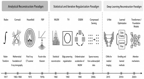
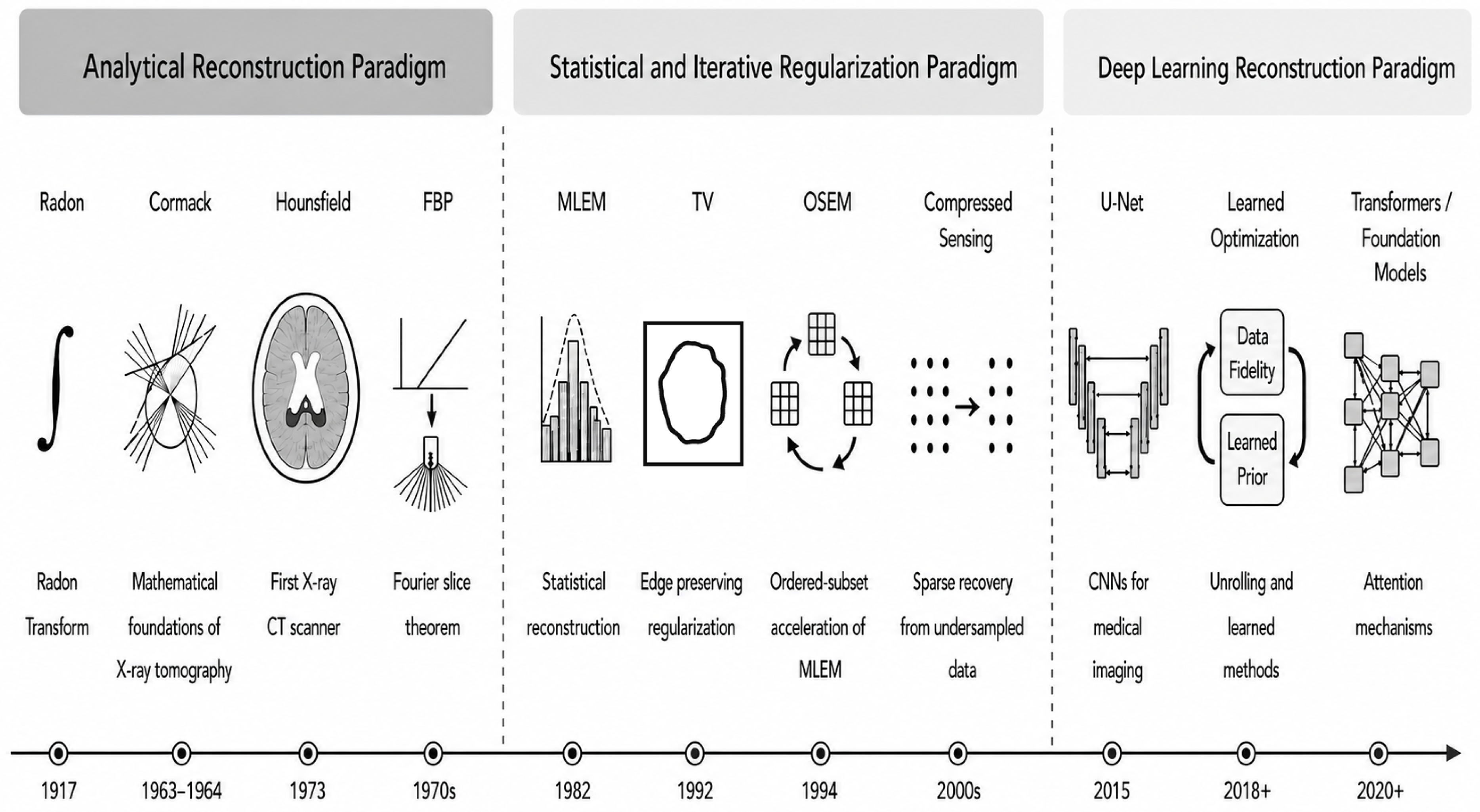
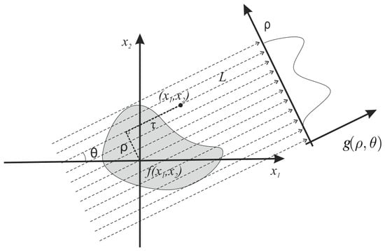
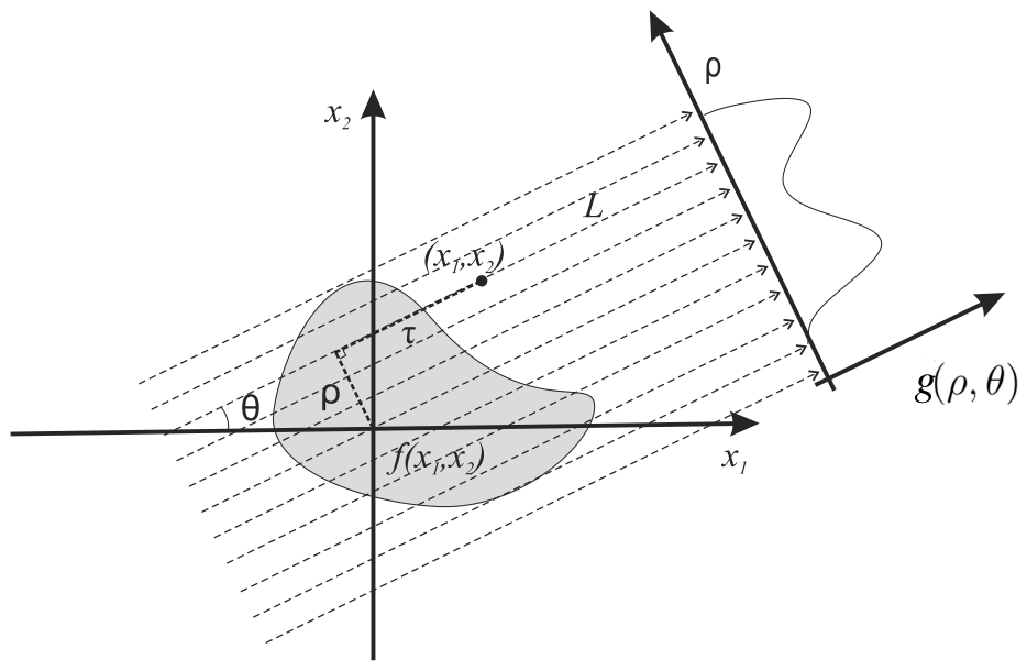

Disclaimer/Publisher’s Note: The statements, opinions and data contained in all publications are solely those of the individual author(s) and contributor(s) and not of MDPI and/or the editor(s). MDPI and/or the editor(s) disclaim responsibility for any injury to people or property resulting from any ideas, methods, instructions or products referred to in the content. |
© 2026 by the authors. Licensee MDPI, Basel, Switzerland. This article is an open access article distributed under the terms and conditions of the Creative Commons Attribution (CC BY) license.