


Abstract
Text that accumulates over time does not only drift: topics are born, they die, they fragment into competing sub-narratives (splits), and they fuse into broader frames (merges). Our companion system paper, BERTilda, detects these events with transparent similarity and flow rules and validates them against human annotators; the present article is its mathematical companion. We show that the forward (outflow) and backward (inflow) coverages used by BERTilda are two semi-couplings between the topics of adjacent windows, both one-sided limits of a single unbalanced optimal-transport problem. The transport view separates the modeling layer from the readout layer: the plan is governed by three interpretable transport parameters, a blur and two marginal fidelities, and by a cost matrix fixed by the embedding geometry, while lifecycle labels are read from two explicit decision levels for survival and dominance. Because the plan is a stable function of that geometry and the topic centroids concentrate around their latent positions, we obtain finite-sample guarantees that account for the noise in the centroids themselves, not just in document attribution. We prove that the recovered transport structure converges to the latent geometry and that labels are recovered once their margin exceeds the plan’s perturbation radius; a lower bound for an edge-decision subproblem shows that the resulting inverse-square dependence on the decision margin cannot be improved in general. The theory also offers an explanation of BERTilda’s empirical pattern: continuation and disappearance are easy, while split and merge have the smallest attainable margins.
Keywords:
topic evolution; temporal graphs; split and merge detection; explainable topic modeling; optimal transport; unbalanced transport; finite-sample stability MSC:
49Q22; 68T50
1. Introduction
A corpus that is collected over months or years carries two very different kinds of change. There is a gradual drift, in which the words attached to a theme shift slowly while the theme itself persists, and a discrete reorganization, in which a theme appears out of nothing, disappears, splits into two, or absorbs another. In political communication, in legislative speech, and in social-media discourse, it is the discrete reorganizations that usually carry the story: a single debate that splits into a geopolitical strand and a domestic strand, or two separate conversations that suddenly fuse around one event.
In a companion paper, published in the proceedings of ECML-PKDD 2026, we introduced BERTilda [1], a framework that makes these discrete events explicit. Topics are discovered independently inside each time window with a snapshot topic model (BERTopic [2] in our instantiation, although the framework is model-agnostic), and then topics in adjacent windows are linked into a temporal graph. A link is supported by two signals: semantic similarity between topic representations, and a bidirectional coverage signal that measures how documents flow from one window to the next. Transparent rules then label each topic as a continuation, a split, a disappearance, a merge target, or as unclear. On a human-annotated subset of U.S. congressional tweets, BERTilda reached majority-agreement rates up to and the best macro-average agreement among the methods we compared.
This article does something different. It does not propose a new system or a new experiment. It asks a question that an applied paper has no room to answer: what is a topic split, mathematically? When BERTilda computes two coverage numbers and compares them to thresholds, what underlying quantity is it estimating, and under what conditions is its verdict reliable rather than a coincidence of finite samples? A rule that works is not the same thing as an explanation of why it works, and the gap between the two is where a mathematical companion is useful.
Our central finding is that all of this can be organized around one object. We first observe that the two coverage numbers are not two unrelated heuristics but two one-sided couplings, that is, two joint distributions linking the old topics to the new ones, each honoring only one of the two marginals exactly. One gets the source side right and distorts the target side; the other does the opposite. We then show that both are extreme, one-sided limits of a single even-handed problem: unbalanced optimal transport between the topics of the two windows. Every lifecycle event turns out to be a shape in its plan. A continuation is a row that puts its mass on one column; a split is a row that spreads its mass; a merge is a column fed by several rows; a disappearance is a row whose mass is simply not transported anywhere. The transport formulation separates two decisions that were interwoven in the rule system: the construction of a flow, governed by a geometric cost and three transport parameters, and the reading of events from that flow, governed by two explicit readout levels.
The transport view is more than a tidier description. It also lets us state rigorous guarantees about where the randomness lives. The reliability of the method depends on two distinct sources of noise: the documents we observe and the topic centroids, which are themselves computed from those documents. The transport plan is a stable function of the geometry, in a sense we make precise, and the centroids concentrate around their latent positions as topics grow. Combining the two, we prove that the recovered transport structure converges to the structure of the latent geometry, and that lifecycle labels are recovered exactly once their margin is larger than the plan’s perturbation radius after the appropriate row- or column-normalization. A lower bound for a single edge-decision subproblem shows that the resulting inverse-square dependence on the margin cannot, in general, be improved, even before the full lifecycle problem is considered. The same analysis is consistent with the empirical ranking reported for BERTilda: continuation and disappearance are robust, while split and merge have the smallest attainable margins.
1.1. Research Gap and Objectives
Three things are missing from the literature reviewed in Section 2. The methods that align topics across windows, by overlap counting, one-to-one assignment, a smooth generative chain, or Gromov–Wasserstein matching (Section 4.2 examines each), come with no finite-sample guarantee for the lifecycle labels they produce. Optimal transport has been used in topic modeling to compare documents and to align sets of equal mass, but not as a model of lifecycle events, in which mass is created at a birth and destroyed at a disappearance. And no existing analysis of alignment accounts for the fact that the topic representatives are themselves estimated from the documents whose flow is measured. The companion system is the instance on which we work; the gap belongs to the field.
The article pursues five objectives.
- (O1)
- To identify what the forward and backward coverage rules estimate, and when one of the two directions would be redundant (Section 4).
- (O2)
- (O3)
- To define the five lifecycle events, including the previously implicit birth, as properties of that plan, with two interpretable readout levels (Section 6).
- (O4)
- To prove finite-sample guarantees that account for the noise in the centroids (Section 7).
- (O5)
- To explain why split and merge are empirically harder than continuation and disappearance, and to check the explicit parts of the theory against the companion settings (Section 8).
Figure 1 ties each objective to the section that meets it.
Figure 1.
The route of the paper: six stages, one per section, from the coverage rules of the system to the guarantees and back to the data. The unshaded boxes build the objects; the two shaded boxes state the results and confront them with the companion experiments.
1.2. Scope
We do not attempt a probabilistic theory of the snapshot clustering step itself. The behavior of a density-based clusterer on real high-dimensional embeddings is genuinely hard to characterize, and a careful paper should target the layer where clean statements are possible. Our guarantees are therefore conditional on the realized partition into topics, under an idealized model in which the documents of each topic are independent draws from a topic-conditional distribution. They are, however, not conditional on the centroids: the centroids are estimated, and our analysis treats them as such. This distinction matters: the theory studies the alignment layer once topics have been formed, not the statistical consistency of the clustering algorithm itself. Section 9.2 returns to this assumption, and Appendix C shows the effect of a perturbed partition on a synthetic example.
1.3. How to Read This Paper
The article is written for a reader who is comfortable with mathematical notation but is not a specialist in optimal transport or concentration of measure. We use two visual conventions to help. A teal box marked Reading restates a formula/expression in plain words. An amber box marked If we skipped this explains what would go wrong if the construction we just made were omitted. We also try, before each theorem, to say why we are about to prove it.
Figure 1 shows the route: six stages, one per section, from the coverage rules of the system to the guarantees and back to the data. In the terms of an empirical article, Section 3, Section 4, Section 5 and Section 6 build the objects and play the role of the methods, Section 7 and Section 8 state the results and confront them with the companion experiments, and Section 9 discusses scope and limitations; proofs, computation, and the synthetic illustration are in the appendices.
2. Background and Related Work
Three established lines of research come together in this paper. Most of the machinery we rely on was developed by others, and we have tried to acknowledge that throughout; our contribution is the synthesis itself, not the parts.
2.1. Topic Models and Their Temporal Extensions
Latent-variable topic models represent documents as mixtures over latent components, from probabilistic latent semantic analysis [3] and latent Dirichlet allocation [4] through matrix factorization [5] and Bayesian nonparametric [6] variants; see [7] for a survey on the area. Temporal extensions encourage the topic parameters to evolve smoothly, as in dynamic topic models [8], topics over time [9], and neural variants such as the dynamic embedded topic model [10]. A different family discovers topics independently in each window by clustering contextual embeddings, as in Top2Vec [11] and BERTopic [2] (the embedded topic model [12] works in the same space, but as a generative model); this snapshot family is what our companion system builds on. Evaluating topics is itself complex: automatic coherence correlates only imperfectly with human judgment [13,14,15,16], which is why the companion paper leans on human validation and why we treat such scores cautiously here.
2.2. Cluster Evolution and the Lifecycle Vocabulary
The vocabulary of discrete lifecycle events, continuation, split, merge, birth, and death, predates topic modeling and was made precise for evolving clusters and communities. Evolutionary clustering balances snapshot fit against temporal smoothness [17]; the MONIC framework cataloged cluster transitions including survival, split, absorption, and disappearance [18]; the study of overlapping communities quantified birth, growth, merging, and death [19]; and community-tracking methods match clusters across snapshots by overlap [20]. Alluvial and flow maps visualize the resulting branching and convergence [21]. Our companion system places these events on snapshot topics; the present paper reinterprets them through optimal transport, so that a split or a merge becomes a property of the transport plan itself. Section 4.2 examines why this overlap machinery cannot simply be transplanted to snapshot topics, and what can.
2.3. Optimal Transport and the Tools We Borrow
Optimal transport originates with Monge and was relaxed to a linear program by Kantorovich [22]; see also [23,24]. Entropic regularization makes transport scalable through the matrix-scaling iteration of Sinkhorn [25,26], and unbalanced formulations relax the conservation of mass [27,28,29], which is what lets transport express birth and death; the statistical behavior of the entropic plan has also been studied [30]. At the document level, transporting the word embeddings of one document onto those of another underlies the Word Mover’s Distance [31], and assigning each point to its nearest centroid is the semi-discrete (power-diagram) limit of transport [32]. Our guarantees rely on standard concentration of measure [33,34,35] and on the two-point method for minimax lower bounds [36,37,38]. Finally, the snapshot partition we condition on is, in practice, produced by density-based clustering [39] on a dimensionally reduced embedding [40], computed with contextual sentence encoders [41,42,43].
3. Setup and Coverage Rules
We keep the notation light, introducing only what we need.
3.1. Windows and Snapshot Topics
Let D be a corpus of N documents, each carrying a timestamp. We slide a window of length along the timeline in steps of , producing windows , and we collect into the documents whose timestamp falls inside window t. Inside each window, a snapshot topic model returns a set of topics and assigns every document to one of them; we write for the documents of window t in topic k, and for its size, the topic’s mass. Writing for the total number of documents in window t, the masses normalize to two probability vectors: over the topics of a window and over those of the next. The pair will be the two marginals of every object in this paper.
3.2. Embeddings and Centroids
A fixed encoder maps every document to a vector , the same encoder across all windows, so that vectors from different windows live in one space (in practice, a contextual sentence encoder [42], here the MiniLM variant [43] built on BERT [41]). Each topic is summarized by its centroid,
and the proximity of two topics in adjacent windows is the cosine of their centroids, .
| Reading. Equation (1) says a topic is represented by the average position of its documents in meaning-space. Because the same encoder is used everywhere, two centroids from different weeks can be compared directly, and a high cosine value indicates that the two topics lie in the same semantic region. |
3.3. The Two Questions
Semantic similarity alone cannot resolve who-came-from-whom. Two topics can have nearby centroids simply because their regions of meaning overlap, even if their documents behave quite differently. So we attribute documents across the window boundary in both directions, because there are two natural, genuinely different questions to ask.
Where did a topic go? For each document of a source topic k, find the closest topic in the next window, accepting the match only if the cosine clears a floor , which we call the document floor. The outflow coverage is the fraction of k’s documents that land in target j:
Where did a topic come from? Symmetrically, for each document of a target topic j, find its closest topic in the previous window. The inflow coverage is the fraction of j’s documents that trace back to source k:
| Reading. The outflow is normalized by the source size: it answers “of the documents that were in k, what fraction moved to j?”. The inflow is normalized by the target size: it answers “of the documents that are now in j, what fraction came from k?”. They divide by different totals, so they are not the same number, and that difference is the whole point of looking in both directions. |
Figure 2 shows the two directions side by side. We will use a single small example throughout the next two sections, so let us state it now.
Figure 2.
The two questions. (Left) forward attribution sends each source document to its closest target topic and normalizes by the source mass, giving the outflow. (Right) backward attribution sends each target document to its closest source topic and normalizes by the target mass, giving the inflow. The two directions look at different documents and divide by different totals.
Example 1
(two sources, one target). Two source topics feed one target. Topic has 1000 documents, topic has 100, and the target j has 500. Suppose half of each source’s documents have j as their closest target, so . Looking backward from the target, suppose of its documents trace to and to , so and .
4. The Coverages as One-Sided Couplings
The path we want to follow starts from a small change of viewpoint. Instead of looking at the coverage numbers one at a time, let us collect the raw counts into a table.
For the forward direction, write for the number of source-k documents whose closest target is j, accepted only when the cosine clears the document floor; documents of k with no acceptable target are collected in a reservoir column , so that every source document is counted exactly once. Dividing the whole table, reservoir included, by the total number of source documents turns it into a joint distribution over (source topic, target-or-reservoir) pairs,
The forward direction has a twin. Write for the number of target-j documents whose closest source is k (again accepted above the document floor), with a symmetric reservoir row for target documents that trace back to no acceptable source, and normalize by :
The reservoir holds exactly the mass that the unbalanced transport plan of Section 5 will later allow to appear or vanish; including it here is what lets both marginals hold with equality despite the floor .
| Reading. A coupling of and is a joint distribution whose row sums are and whose column sums are , that is, one that honors both marginals at once; each table here honors only one. As before, is the distribution of mass over the old topics and the distribution over the new topics. The forward table has the correct old-topic marginal (every source document is placed somewhere, so the rows add up to the source sizes), but its column sums are whatever happens to fall out. The backward table is the mirror image: correct new-topic marginal , distorted rows. We therefore call them one-sided couplings, also known as semi-couplings in the unbalanced-transport literature [27]: each pairs one true marginal with the free measure that the attribution induces on the other side. Reading along a row of and renormalizing recovers the outflow coverage; reading down a column of and renormalizing recovers the inflow coverage. |
So forward and backward coverage are two one-sided couplings between the same pair of topic sets, each respecting one marginal exactly and bending the other. The natural question is now sharp: do they ever hold the same counts? If they did, we could throw one away.
Proposition 1
(when one direction would be redundant). The pseudo-inflow , obtained by rescaling the outflow by the mass ratio, equals the true inflow if and only if
that is, if and only if the number of source-k documents that flow forward to j equals the number of target-j documents that flow backward to k.
Proof.
By definition , while . The two are equal exactly when their numerators agree. □
| Reading. Condition (6) is a balance condition: the forward count and the backward count must match cell-by-cell. There is no reason for them to. Forward attribution looks at the source’s documents and asks which target centroid is nearest; backward attribution looks at the target’s documents and asks which source centroid is nearest. These are two different sets of documents, judged against two different sets of landmarks, so, in general, , and the inflow carries information the outflow does not. |
Example 2
(continuing Example 1). The forward counts are and . The pseudo-inflow rescales these by the target size: and . The large source appears to supply the entire target, purely because it is large. The backward counts are and , giving and . Since , the balance condition (6) fails, and the pseudo-inflow is badly wrong: it would have declared a merge dominated by the big source, while the true inflow shows two comparable contributors. The remaining of the target’s documents trace back to no acceptable source and fall in the reservoir, so the backward column still sums to the full target size of 500.
| If we skipped the backward direction. We would be forced to invent an inflow from the outflow, and the only mass-consistent way to do that is the pseudo-inflow. As the example shows, the pseudo-inflow is dominated by source size, so a large but only loosely related topic would masquerade as the principal origin of a target. BERTilda’s requirement that both coverages clear a threshold is precisely a test against this failure: it asks for the cell to be heavy in both tables, which can only happen when and are both large, that is, when the two directions agree on a genuine flow. |
Figure 3 draws the two tables for the running example, with their marginals.
Figure 3.
The two one-sided couplings of Example 1, as raw counts. The forward table gets the row sums right (the source sizes), and the backward table gets the column sum right (the target size), but the individual cells disagree (). This cell-level disagreement is the content of Proposition 1: the two directions are different tables, so each carries information the other lacks. Only the column of target j is drawn; the row sums also count documents sent to other columns and to the reservoir.
4.1. Taking Stock: What Any Repair Must Provide
The two tables of this section are each half right, and Proposition 1 says that neither can be rescaled into the other. Something has to repair them. We first list the requirements that any repair must satisfy; each follows from material already presented.
- (R1)
- Identity-free linking. The documents of window are not the documents of window t: when the step is at least the window length, the two sets are disjoint, and even when the windows overlap, the shared documents are an artifact of the windowing, not the phenomenon being tracked. Whatever links the two windows must rest on the shared embedding geometry of Section 3 alone, never on shared membership.
- (R2)
- Even-handedness. The lesson of Proposition 1 is that a construction that privileges one direction silently discards the information carried by the other. The repair must honor both marginals symmetrically, in one object, not two.
- (R3)
- Fractional, mass-weighted flow. A split is one row spreading its mass over several columns, and a merge is one column fed by several rows, so no one-to-one pairing of the old topics with the new ones can be assumed; the two sets do not even have the same size in general. Example 1 adds the second half of the requirement: when sizes are ignored, the pseudo-inflow lets a topic dominate by mere bulk. Flows must therefore be fractional and weighted by document mass.
- (R4)
- (R5)
- Statistical tractability. The centroids are estimates, as Section 3 warned, so every quantity built on them inherits their noise. If the guarantees of Section 7 are to exist at all, the repair must depend on the estimated geometry continuously and quantitatively. A unique optimizer of a strictly convex problem is the natural way to obtain this, and any construction that jumps when two quantities tie is disqualified in advance.
| Reading. Nothing on this list mentions transport. Requirement (R1) comes from how the data arrive, (R2) from Proposition 1, (R3) and (R4) from the event vocabulary itself, and (R5) from the fact that every input is estimated. The list is a checklist distilled from the system’s own behavior, and any candidate framework can now be audited against it. That audit is next. |
4.2. Four Natural Candidates, and Where Each One Stops
Checklist in hand, we walk through the frameworks the literature would offer for this task, in the order in which a practitioner would plausibly reach for them. None of them is a straw man: each is the canonical tool of a neighboring problem, and each stops at a specific line of the checklist. Table 1 summarizes the outcome.
4.2.1. Tracking by Overlap
The classical machinery for cluster evolution matches clusters across snapshots by counting shared members: the MONIC framework reads survival, splitting, and absorption off overlap sets [18], and community tracking quantifies birth, growth, merging, and death the same way [19,20]. On its home ground, this family handles (R3) and (R4) gracefully; lifecycle events were, after all, first made precise here. But its home ground is a persistent population re-clustered over time, and that is the one thing we do not have: by (R1) there are no shared members to count. Transplanting the idea to snapshot topics forces one to replace identity with nearest-centroid attribution, and attribution must choose a direction to attribute in. The result is the two one-sided tables this section started from: overlap tracking, moved to our setting, does not repair the tables, it is the tables, one-sidedness (R2) included, and its thresholded set decisions jump under perturbation, failing (R5).
4.2.2. One-to-One Assignment
The next classical reflex is to treat alignment as a bipartite matching problem: pair each old topic with at most one new topic so that the total centroid cost is smallest, which the Hungarian method solves exactly [44,45]. This candidate is identity-free and even-handed, so (R1) and (R2) hold, and it is the first on the list that optimizes a global objective instead of making local threshold decisions. It stops, hard, at (R3): a matching is one-to-one on its matched part, so a split and a merge are not events the formalism can detect but configurations it forbids; sets of different sizes must be padded with dummy topics; and a topic counts as one unit whether it holds a hundred documents or a thousand. It also fails (R5), because the optimal matching flips discontinuously when two costs cross. The instructive part is what happens when one tries to fix it. The standard cure for the rigidity of matchings is to allow fractional ones, and by the Birkhoff–von Neumann theorem, the fractional matchings are exactly the couplings with uniform marginals [24,46]. Replacing the uniform marginals by the topic masses, which is what (R3) demands, produces word for word the Kantorovich program of Section 5. Repaired at (R3), one-to-one assignment becomes balanced transport, with (R4) and (R5) left open; settling those two is the business of the next section.
4.2.3. Smooth Dynamic Topic Models
A different family changes the topic model instead of aligning its outputs: dynamic topic models chain the parameters of a fixed set of topics through time and ask the chain to move smoothly [8,9,10]. Two facts keep this road from starting here. First, the companion framework is deliberately model-agnostic: the snapshot topics arrive from an arbitrary clustering pipeline, and a generative chain cannot be retrofitted onto a partition it did not produce. Second, and more fundamentally, the design commitments point the other way. A fixed number of chains under a smoothness prior is a model of the gradual drift from the opening paragraph of this paper, with no vocabulary for the discrete reorganizations, split, merge, birth, and death, that are our actual object of study, so (R3) and (R4) fail by design. These models answer a different question altogether; we list them because a reader will rightly think of them, not because they compete on this one.
4.2.4. Gromov–Wasserstein Matching
At the far end of generality, Gromov–Wasserstein matching aligns two sets that live in unrelated spaces by comparing their internal distance patterns [24,47]. It is identity-free, even-handed, and fractional, so it clears (R1)–(R3). But it solves a harder problem than the one we have, and charges for it. Our two windows share one encoder and hence one space, in which the cosine of centroids already prices every pair (Section 3), so the invariance that Gromov–Wasserstein buys is an invariance we do not need. The price is that the objective becomes a non-convex quadratic, uniqueness of the optimizer is lost, and with it goes the quantitative stability that (R5) demands and on which the whole of Section 7 rests. Buying an unneeded generality at the cost of the needed guarantee is a poor trade.
Table 1.
The audit at a glance. The columns are the requirements of Section 4.1: (R1) identity-free linking, (R2) even-handedness, (R3) fractional mass-weighted flow, (R4) open accounting, and (R5) statistical tractability. Each candidate is judged in its standard form; the text of Section 4.2 argues each cell. Smooth dynamic topic models are absent because they redesign the topics rather than align the given ones, so the checklist does not apply to them. The last two rows are built in Section 5: the balanced plan fails exactly at (R4) and (R5), and the two amendments of step 3, the blur and the soft marginals, are the minimal repairs.
| If we skipped this audit. The transport problem of the next section would arrive ready-made, and a careful reader could suspect that the mathematics had been chosen for its elegance and the modeling bent afterwards to fit it. The checklist was forced by the data and by the rules’ own failure modes; each neighboring framework was tried and stopped at a named line; and the two amendments that turn the classical problem into ours, a blur and a pair of soft marginals, are introduced in the next section, one requirement at a time. Unbalanced entropic transport is the only candidate that meets all five. |
The ingredients are standard: couplings driven by a geometric cost, going back to Kantorovich [22,23], made strictly convex and statistically tame by entropic smoothing [26,30], and opened to the creation and destruction of mass by soft marginal penalties [27,28,29]. None of that machinery is ours. The next section builds the object in the order of the requirements.
5. The Unbalanced Optimal Transport Formulation
We now have two lopsided tables: each respects one marginal and distorts the other. What we want instead is a single, even-handed object that honors both marginals as closely as possible and that is driven by the geometry, since the only reason to link two topics is that they sit close in meaning-space. Optimal transport is precisely the theory of such objects, and it is the candidate that passed the audit of Section 4.2. We build it in three short steps, and at each step, we identify what the formula captures and what would be lost without it.
5.1. Step 1: A Cost from the Geometry
Define the cost of associating source topic k with target topic j as one minus their similarity,
| Reading. It is “cheap” to move mass between two topics that mean almost the same thing, and expensive to move it between unrelated ones. The matrix C is the only place the embedding geometry enters; everything downstream depends on the centroids only through C. We will use this fact heavily in Section 7. |
5.2. Step 2: The Balanced Plan, and Its Blind Spot
A transport plan is a non-negative table that says how much mass moves from each old topic to each new one. The classical (Kantorovich) problem [22] looks for the cheapest plan that turns the old distribution exactly into the new distribution ,
| Reading. “Move all of the old mass onto the new mass, paying the semantic distance for every unit moved, and do it as cheaply as possible.” The constraints force the row sums to equal the source sizes and the column sums to equal the target sizes, so this plan is even-handed, where the two coverage tables were each one-sided. |
| Why balanced transport is not enough. The two equality constraints in (8) say that every unit of old mass must be transported and every unit of new mass must be supplied. But a topic that disappears is precisely old mass that goes nowhere, and a topic that is born is new mass that comes from nowhere. The balanced problem cannot represent either: it would be forced to send a dying topic’s documents onto some surviving topic and call it a continuation. To describe lifecycles, we must allow mass to be created and destroyed, at a price. This is requirement (R4), failing in plain sight. |
5.3. Step 3: Blur, and Let Mass Leak
Two changes turn (8) into the object we want. First, we add an entropy term that gently prefers smoother plans; this is the entropic regularization of Cuturi [26], controlled by a parameter that we will call the blur. Second, we replace the two hard marginal constraints with soft penalties, allowing the plan’s row and column sums to deviate from and , at prices and , the disappearance price and the birth price; this is unbalanced optimal transport [27,28]. The problem becomes
Here, is the vector of row sums and the vector of column sums. Because the row and column sums of an unbalanced plan need not be probability vectors, KL throughout (9) denotes the generalized (unnormalized) relative entropy between non-negative vectors,
with the conventions and if for some i. The two correction terms vanish when a and b have equal total mass, so (10) reduces to the ordinary relative entropy when both arguments are probability vectors.
The two prices are kept separate on purpose: the disappearance price sets how strictly the old masses are conserved and the birth price how strictly the new ones are, so that the asymmetric limits used in Section 5.4 are well posed. For and with positive marginals, the objective in (9) is strictly convex and coercive in P, so the minimizer exists and is unique [27,28]. Two notational conventions will keep later statements light: the marginals are fixed by the partition throughout, so the solution map displays only its dependence on the cost; and when the distinction between the two penalties is immaterial, we write , with statements such as meant componentwise.
| Reading, term by term.(a) pays the semantic distance for transported mass, as before. (b) prefers diffuse plans over needle-sharp ones; sharpened away, the blur recovers sparse plans, and enlarged, it smears mass over many cells. (c) no longer forces every old topic to ship all its mass; it penalizes a deviation from it instead of forbidding it. A source topic is now allowed to keep mass un-transported, that is, to disappear, at a cost set by the disappearance price. (d) is the mirror image and lets new mass appear without a source, that is, lets a topic be born, at a cost set by the birth price. As the two prices grow without bound, the penalties become infinitely steep, and we return to the balanced entropic problem; removing the blur as well recovers the classical unregularized Kantorovich problem. |
| If we dropped the blur (b). With the blur removed, the plan becomes sparse and need not be unique, and such plans are brittle: a document, or a centroid, sitting on the boundary between two regions can be flipped from one side to the other by an arbitrarily small change. We will see in Section 7 that the blur is what buys the stability that requirement (R5) asked for, and that the price of stability is a controlled bias. |
Figure 4 draws the whole construction as a picture: two priced flows across the window boundary, plus one priced leak on each side.
Figure 4.
The unbalanced transport problem (9) as a picture. Two bands carry mass from old topics (left) to new topics (right); each pays the semantic distance (a) and is spread rather than needle-sharp by the blur (b). The short topic keeps its mass un-shipped, a disappearance (c), and the dashed topic receives mass with no source, a birth (d). Each leak is priced by and rather than forbidden. The arrowheads land on different target faces to keep the two flows legible; the picture is schematic, not a specific plan.
BERTilda’s labeling stage used several event-specific thresholds: a topic-similarity floor, document and topic coverage thresholds, and four event thresholds, in practice read differently in the inflow and outflow directions. The transport formulation (9) does not make all decisions threshold-free. Rather, it separates them. The transport layer is governed by three numbers with clear meanings, the blur and the two prices, together with a cost matrix that is not a free parameter at all but is read off the geometry by (7). The readout layer, introduced in Section 6, then uses two global decision levels, survival and dominance, to turn the plan into labels. This is the sense in which the transport view is simpler: it replaces a collection of case-specific rules by a geometric flow plus a small number of explicit, interpretable choices.
5.4. BERTilda as a One-Sided Limit of the Transport Problem
Before reading lifecycles off the plan, we make the promised connection precise, because it is the bridge between this theory and the system that motivated it.
Recall forward attribution from (2): each source document is sent to its single closest target centroid, with no constraint on how much each target receives, and the assignment is hard. In the language of (9) this is the corner
applied at the level of individual documents, not topic centroids. The document floor is itself an unbalanced feature: the floor is a reservoir column of constant cost , left free by , which receives a document when every target is farther. Backward attribution is the symmetric corner, with the roles of source and target exchanged.
| Reading. BERTilda computes the two extreme, one-sided limits of the transport problem: one keeps the source side faithful and lets the target side float (the outflow), the other does the reverse (the inflow). Its bidirectional rule, demanding that both coverages be extensive, is asking for the cell to survive both limits at once. We read the even-handed plan, with a finite blur and finite prices, as the object these two limits bracket, and the agreement between the two directions as an approximation to it. This reading is not proved here. |
There are, in fact, two granularities of the same idea, and both deserve a name. The topic-level plan uses the cost (7) between centroids and the two marginals; it is coarse but cheap, and it is the object we analyze formally in Section 7. The document-level plan uses costs between individual document embeddings and topic centroids (a relative of the Word Mover’s Distance [31], which transports word embeddings between two documents); it is finer, and BERTilda’s coverages are its hard, one-sided limit (with the reservoir column above), which is the semi-discrete or power-diagram regime of transport [32]. The two levels agree in clean, well-separated cases, but they are not identical objects. The guarantees below are stated for the topic-level plan; the document-level analog follows under the same cost-perturbation mechanism once the document-to-centroid costs are softened, not made hard. We return to this distinction in Remark A2.
6. Reading Lifecycles off the Plan
We can now define the lifecycle events directly as shapes of the plan, without separate event-specific thresholds. Two summaries are enough, and they make sense for any non-negative plan P; in this section, is the computed plan. For a source topic k, write its transported mass as
and order the renormalized row, writing for the largest, second-largest, and so on among the shares , defined when ; we will call the top share and the runner-up share. The column side is treated symmetrically: the transported mass of a target and its ordered column shares are
We then fix two explicit readout levels, separate from the blur and the prices: a survival level and a dominance level . The pair of levels is the transport-side counterpart of the four event thresholds of the system paper: one global survival level and one global dominance level replace the four event-specific ones, so the values validated there translate directly.
| Reading. Of everything a topic owns, the plan ships some mass, not necessarily less than it owns; survival asks whether the ratio clears the survival level. Dominance asks whether the largest single destination holds enough of what was shipped. Two numbers per topic, the top share and the runner-up share, are all the readout ever looks at, and they separate a clean continuation from a clean two-way split. |
Definition 1
(lifecycle events as shapes). Fix and . A surviving source, one with , is labeled
- continuation if a single target dominates, ;
- split if no target dominates but a second one is substantial, and ;
- unclear otherwise, that is when and (the mass is shattered into many small pieces).
A source with is a disappearance. Symmetrically on columns, a surviving target () is a merge if and , a continuation-target if , and unclear otherwise; a target with is a birth.
| Why the runner-up, and why . Using only the failure of dominance would call every non-dominant row a split, including one whose mass shatters into many tiny fragments, which is ambiguity rather than a two-way split. Requiring a substantial runner-up, , keeps a genuine split apart from that noise and sends the noise to unclear. Taking orders the two levels, , so that “dominant” and “substantial second” do not overlap; in particular, a continuation’s dominant target () leaves less than for the rest, so exactly one of continuation, split, unclear applies to each surviving source. |
Figure 5 shows a single plan with all the events visible at once.
Figure 5.
Every lifecycle is a shape in one plan. Row puts its mass on a single column (continuation); row fans its mass across two columns (split); row has a small total (disappearance); column (outlined) collects mass from two rows (merge). Birth would be a column with a small total. The labels follow Definition 1 from two numbers, the survival level and the dominance level . The cell values are schematic (, so that each row sums to its survival ratio), not the entries of a computed plan.
Birth, Unclear, and the Small Topic
Two of the target labels, birth and unclear, are easy to confuse, so the target side of Definition 1 deserves to be spelled out. A birth is a column whose survival is below , whatever its shape: most of the mass that j owns had to be created at the birth price. A column that survives is sorted by shape alone: dominated by one source if , a merge if no source dominates but the runner-up is substantial, , and unclear otherwise, when its mass arrived in many small pieces. The boundary between birth and unclear is therefore the survival level alone: an unclear column has received its mass, and the plan cannot attribute it, whereas a birth has not received its mass at all. Figure 6 draws the two decisions.
Figure 6.
The two decisions on the target side (, ). (Left) survival first; a column receiving less than a fraction of its mass is a birth, whatever its shape. The marked point is the small topic of Example 3. (Right) shape second, for surviving columns, in the plane of top share against runner-up share (a triangle, since and ): dominated, merge, and unclear meet at the corner . Birth and unclear are never neighbors here, because the birth decision is made on the left.
Example 3
(a small target near the survival level). Take and two target topics with the same population survival : both are births with margin (Definition 2 below). One holds 60 documents in a window of 3000, so ; the other holds 600, so . Theorem 2 guarantees the label when the plan error is at most with : for the small topic against for the large one. The lower bound of Theorem 3 gives a point of comparison for a coverage decision of the same size: with 60 documents, and , no test resolves a margin below . We do not show that this bound applies to the survival ratio.
Size does not make a topic a birth, since survival is normalized by the topic’s own mass; it makes the verdict less reliable, and a small column near is the least reliable verdict in the vocabulary, on either side of the level. The margin of Definition 2 covers the unclear label too, so Theorem 2 also says when an unclear verdict can be trusted. We have a clean object, the plan, and a clean way to read events off it. But this plan is built from the cost (7), which is built from the centroids (1), which are estimated from a finite and noisy sample of documents. Nothing we have said so far tells us whether the picture in Figure 5 is a faithful image of the underlying reality or an artifact of the particular documents we happened to collect. Section 7 addresses this question.
7. Finite-Sample Guarantees
7.1. Two Sources of Randomness and a Target
It helps to separate the two ways the world could have come out differently.
- Attribution noise. Even with the centroids fixed, we observe a finite set of documents, and the coverage numbers are sample fractions that would wobble if we drew a different sample.
- Centroid noise. The centroids themselves are sample averages, so a different sample would have placed the landmarks slightly differently, which moves the costs and hence the plan.
A natural first approach would control only the first source by treating the centroids as fixed and conditioning on them. That move is tempting but not quite rigorous, because the centroid is the average of the very documents whose flow we then study; one cannot both hold the average fixed and treat the sample as freely random. Worse, it makes the target of the analysis strange: one ends up proving recovery of the edge set one would obtain with infinitely many documents, but the same finite-sample centroids, which is not a population object at all.
| Reading. We want our theorems to be about the latent geometry, the centroids one would obtain with unlimited data, not about a frozen snapshot of noisy centroids. The transport view makes this possible because the plan is a function of the cost matrix, and we can ask directly how much the plan moves when the cost moves. We therefore condition only on the partition into topics (which fixes the two marginals) and treat the centroids as estimated. |
Concretely, let denote the latent centroid of topic , that is, the mean of its topic-conditional embedding distribution, and let be the cost matrix built from the latent centroids. The population plan is , and the empirical plan is , where is exactly the cost of (7), now written with a hat to stress that it is built from the observed centroids (1) and is therefore estimated. The star thus marks latent objects throughout: , , . Our task is to bound the distance between the two plans.
7.2. The Centroids Concentrate
We first record that a centroid built from more documents is a better estimate of the latent one. We assume embeddings are normalized, , as is standard for the sentence encoders used in practice.
Lemma 1
(centroid concentration). Fix the partition into topics, and suppose that, under the realized-partition model, the embeddings within each topic are independent draws from its topic-conditional distribution. Then, for any , with probability at least , simultaneously for every topic,
where K is the total number of topics across the two windows.
| Reading. The error of a centroid shrinks like one over the square root of the topic’s mass. Bigger topics give sharper landmarks. The logarithm is the small price of asking the bound to hold for all topics at once. The independence assumption is not a claim that HDBSCAN or any other snapshot clusterer is already statistically characterized; it is the conditional sampling model under which the alignment layer is analyzed after the partition has been fixed. |
Lemma 2
(from centroid error to cost error). Suppose every latent centroid has norm at least , and that is large enough that the bound of Lemma 1 is at most r; then, on the event of that lemma, every empirical centroid also has norm at least r. On the same event, with the explicit constant ,
| Reading. If topics are not degenerate (their centroids do not collapse to the origin, which would mean a topic with no coherent direction), then the worst error in any cost entry also shrinks like one over the square root of the smallest topic. The non-degeneracy condition is mild and can be checked on the data, since the empirical centroid norms are observable. |
7.3. The Plan Is Stable in the Cost, and the Blur Controls How Stable
We arrive at the result on which the soundness of everything else depends. We want to know that a small change in the cost produces a small change in the plan. We pause to say why we need it: without such a statement, Lemma 2 would tell us the costs are nearly right but leave open the possibility that the plan, and hence every event label, is wildly sensitive to the remaining error. The theorem rules this out, and in doing so, it reveals the role of the blur.
Theorem 1
(stability of the plan under cost perturbation). Assume that the entries of μ and ν are positive on their supports. By construction (7), every admissible cost matrix lies in the compact cube , so no boundedness assumption is needed. For fixed and , the map is Lipschitz on that cube: there is a finite constant , depending on ε, μ, ν and ρ but not on the pair of costs, such that for any two cost matrices ,
The displayed factor is the explicit part of the ε-dependence, extracted from the Gibbs kernel; the behavior of itself as is discussed in the remark that closes the proof in Appendix A.
Proof of Theorem 1.
The plan can be written entry-wise as for potentials that solve the unbalanced Sinkhorn fixed-point equations [26,27]. On the cube with positive marginals, these potentials remain bounded (in the unbalanced problem, the finite marginal penalties fix their scale, so there is no additive gauge to quotient out), and the Sinkhorn map is differentiable [29,48]. A perturbation of the cost enters the logarithmic kernel as ; differentiating the optimality system therefore gives a first-order change of size in the log-plan, with the remaining constant controlled by the marginals and for each fixed . Since the total transported mass is bounded in the unbalanced problem, converting from log-plan to plan entries and summing gives (15). Appendix A records the argument in the form needed for the subsequent bounds; the exact numerical value of is not used. □
| Reading. For a fixed blur, the plan reacts to a cost error by at most a factor of order , one over the blur. Blur a lot, and the plan barely moves when the geometry wobbles: it is stable. Sharpen toward hard assignment, and the guarantee weakens (Remark A1). |
| The trade-off this exposes. A heavy blur is stable but smeared: it biases the plan toward the product table , washing out genuine structure. A light blur is faithful to the geometry but fragile. There is therefore a real tension, set by the blur, between stability and sharpness. This is not a defect of the method; it reflects the fact that a hard nearest-centroid assignment, the regime BERTilda actually uses, is the end of the family where the guarantee is lost. Figure 7 makes the trade-off visible. |
Figure 7.
The blur parameter trades sharpness for stability. A near-zero gives an almost sparse plan that mirrors the geometry closely but can flip at the slightest perturbation; a larger gives a smoother plan that barely reacts to noise but is biased toward the product table. BERTilda’s hard assignment lives at the fragile left end.
Combining the three results is now immediate, and gives the population-level guarantee we were after.
Corollary 1
(the empirical plan tracks the latent geometry). Under the assumptions of Lemmas 1 and 2, for fixed ε and ρ, with probability at least ,
| Reading. Provided topics are reasonably large, and we do not push the blur to zero, the transport plan we compute from the data is close to the plan determined by the true geometry. The error shrinks as topics grow and grows as we sharpen. This is the statement that the condition-on-the-centroids approach could not make: the noise in the centroids is inside the bound, not assumed away. |
Remark 1
(a perturbed partition enters through the cost, and through the marginals). The guarantees above hold for a fixed partition (Section 1.2), but the transport view says how a change of partition acts. If a topic loses at most a fraction of its documents and gains at most new ones, then, the embeddings being unit vectors, its centroid moves by at most
(proof in Appendix A). If the centroids have norm at least , the mean-value bound in the proof of Lemma 2 moves every cost entry by at most , and Theorem 1 moves the plan, for fixed marginals, by at most . The masses move too, by at most q in over a window; Theorem 1 does not cover this, but the plan depends on the marginals through the same fixed-point system, so the implicit-function argument of Appendix A makes it continuous in them as well, with a constant we do not quantify. A perturbed partition is thus a first-order perturbation of the inputs, and Theorem 2 says which labels survive it: those whose margin exceeds the induced decision error. Appendix C shows both effects on a synthetic example.
7.4. Lifecycle Labels Are Recovered Above an Explicit Margin
A bound on the whole plan is more than we need for any single label. A label depends only on a margin, the gap between the relevant quantity (a row sum, or a dominance share) and its decision level. We now make precise the intuition that a label is safe exactly when its margin beats the plan’s wobble; Figure 8 draws the condition on a line. We state it for one source label; the target case is identical, with rows and columns exchanged.
Figure 8.
The recovery condition (19), on a line. The population value sits a margin above (or below) the decision level. The empirical decision value carries a wobble bounded by the plan error of Corollary 1 multiplied by the sensitivity factor in Definition 2. As long as this decision wobble is at most half the margin, the empirical value lands on the same side of the level as the population value, so the label is correct.
Definition 2
(label margin and decision sensitivity). For a source topic k with population label ℓ, evaluated on the population plan , the margin is the smallest distance from the deciding quantities to their levels:
with the merge, birth, and unclear-target cases obtained by replacing by the column quantities . All four source labels are decided by the same three quantities, so a margin is available for each of them, including unclear, whose margin measures how far the shattered row is from qualifying as a continuation or a split. Because the deciding quantities include normalized shares, plan error must be converted into decision error. For a source topic, we use the conservative sensitivity factor
and for a target topic the analogous factor . Because , this single factor also dominates the sensitivity (respectively ) of the survival ratio, so no separate constant is needed for it.
Theorem 2
(exact label recovery). Fix ε and ρ, and let a source topic k have population margin and sensitivity . If the plan error is small enough after this normalization,
then the empirical label of k equals its population label. The same statement holds for target labels with . In particular, by Corollary 1, the source statement holds with probability at least as soon as
Proof of Theorem 2.
A row or column sum changes by at most the change in the plan, but the normalized shares are not globally 1-Lipschitz because the denominator can be small. For a surviving population source, ; because the margin includes the survival gap, the hypothesis also keeps the empirical row sum above , and the share vector changes by at most . Sorting is non-expansive, so the largest and second-largest shares inherit the same bound. Thus, every deciding source quantity changes by at most . If this is at most , no deciding quantity crosses its level, and the label is unchanged. Substituting (16) gives (20). Details are given in Appendix A. □
| Reading. A label is recovered when it is comfortably away from the boundary between two interpretations, where “comfortably” is measured in units of the decision error induced by plan wobble. The sample size (20) says everything one would expect: more data helps (the ), a clearer event helps (the ), sharpening the blur hurts (the ), and very small topics hurt through the sensitivity factor . An event sitting right on the boundary, , is genuinely undecidable, and the bound correctly refuses to promise anything. |
7.5. The Difficulty Is Intrinsic: A Lower Bound for an Edge Decision
The full lifecycle problem contains row sums, column sums, and order statistics of a transport plan. Nevertheless, a coverage-based method such as BERTilda must, in particular, be able to solve the simpler subproblem of deciding whether one empirical coverage lies above or below a threshold. The next result shows that the dependence on the margin already appears in this elementary subproblem. Thus, the margin dependence in (20) is the one to expect, although this theorem is not a full minimax lower bound for the complete lifecycle pipeline.
Theorem 3
(edge-decision lower bound). Fix and assume . Consider deciding whether a single coverage exceeds its threshold τ, when the true coverage is either or . For any , any test based on n attributed documents that is correct with probability at least in both cases must use
documents.
Proof of Theorem 3.
The two candidate worlds differ only by in one Bernoulli parameter. On any interval bounded away from 0 and 1, the KL divergence between the two Bernoulli laws is of order . A two-point testing bound, therefore, forces to be at least logarithmic in ; Figure 9 shows the geometry of the argument. The full computation is in Appendix A. □
Figure 9.
Why the lower bound (21) holds, as a picture. The measured coverage is a sample mean, so under each candidate world, it follows a bell-shaped law: centered at if the truth is below threshold, at if it is above. The two laws are only apart, and they overlap (shaded); a measurement falling in the overlap could have come from either world, which is the unavoidable error. The width of each law is of order , so the overlap becomes small only once , that is, once . No test, however clever, can separate laws that overlap this much with fewer samples.
| Reading. The in the cost of recovery is not an artifact of transport, of Sinkhorn, or of our particular estimator. It already appears in the simplest threshold decision that a coverage-based lifecycle method must be able to make. Our upper bound (20) has the same margin scaling, with additional factors for blur and normalization. The result should therefore be read as a sharpness check on the margin dependence, not as a proof that the full transport labeling pipeline is globally minimax optimal. |
8. Comparison with the BERTilda Results
A useful theory should explain observed behavior and point to what should remain true beyond one corpus. The companion paper reports, on a balanced human-annotated set of 120 congressional events, validated precisions of for continuation, for disappearance, for split and for merge, together with a threshold-sensitivity study in which split and merge were the most sensitive to small changes and disappearance the most stable. The transport analysis is consistent with this ordering and predicts that the same pattern should appear whenever split and merge events have smaller margins than continuation and disappearance events.
8.1. Continuation and Disappearance Have Large Margins
A continuation is a row concentrated on one column, and a disappearance is a row whose total is small. By Definition 2, these are decided by quantities, a dominant share well above or a survival ratio well below , that are typically far from their levels: a surviving topic that genuinely continues sends almost all its mass one way, and a topic that genuinely dies sends almost none anywhere. Large margins mean, through Theorem 2, reliable labels.
8.2. Split and Merge Have the Smallest Margins
A split is a row whose mass is shared by two or more comparable targets, and a merge is the same down a column. By construction, these are the configurations in which several cells are close in value, which is where a small change in cost can tip mass from one cell to another. The readout levels also cap the margin of a split or a merge at , the smallest cap among the labels (Table 2). Because BERTilda uses a hard assignment (the fragile left end of Figure 7), the transport view suggests that its split and merge labels are the least stable, and the threshold-sensitivity study is consistent with this.
Table 2.
The explicit parts of the theory at the companion settings (, ): the largest margin of each label, the sensitivity converting plan error into decision error (survival factor from the proof of Theorem 2), and the plan error that still guarantees the label, for an average topic () and a floor topic (). Target labels use .
8.3. The Backward Direction Helps Disappearance Specifically
The system paper found that adding backward attribution helped most for disappearance, and the reason is now mechanical. The forward-only view sees only the rows of the plan, so a large source with some mass near any target can look like a continuation even when that target is dominated by other sources. The column view supplied by the inflow reveals the marginal deficit, that the source’s mass is not in fact being received, which is the signal a disappearance needs. This is the same asymmetry that Proposition 1 isolated, now seen through its effect on one event type.
| Reading. The empirical ranking continuation > disappearance > split > merge is consistent with the theory if it tracks, on average, how far each event type sits from its decision level: labels are reliable in proportion to their margins, and split and merge have the smallest attainable margins. |
8.4. A Numerical Check Against the Companion Settings
The constants and in the sample-size condition (20) are not numerically pinned down by our argument, so that condition is a rate, not a number. Three parts of the theory are explicit, and each can be put against the companion settings: about tweets and 22 topics per window, a floor of 50 documents per topic (relative mass ) against an average topic of at most about 320 (), with , and .
8.4.1. Margins and Sensitivity
The readout levels bound the margin of each label by construction: at most for a disappearance, for a continuation, and for a split or a merge, attained at the even two-way split . Since both bounds scale as , the sample size that (20) requires for the best split is times that of the best continuation and 6 times that of the best disappearance. Table 2 converts the margins into the plan error each verdict tolerates, . Survival-based verdicts have sensitivity (the proof of Theorem 2 bounds the survival quantity by ; the theorem’s single is the conservative common bound), share-based verdicts , four times larger; and a topic at the floor tolerates about six times less plan error than an average one, so label errors should concentrate in small topics.
8.4.2. The Lower Bound
Theorem 3 is fully explicit: with and , no method places a coverage on the correct side of a threshold with probability from 50 documents when the margin is below , or from 320 when it is below . The band the system leaves between its disappearance level () and its continuation level () is fewer than three such margins wide at the floor.
8.4.3. What This Shows
The comparison is consistent with the observed ordering: disappearance and continuation, with the largest margins and the smallest sensitivity, were validated at and , split and merge at and . It does not reproduce the precisions, which depend on the implicit constants, and it orders the four events only as two groups.
9. Discussion and Conclusions
9.1. What the Transport View Buys, and What It Costs
The transport view buys three things at once: a simpler description (a geometric cost and three transport parameters, followed by two explicit readout levels, in place of several event-specific thresholds), a unification (forward and backward coverage as one-sided limits of a single problem, with every event a shape of its plan), and a fair statistical layer (guarantees that include the noise in the centroids). It is fair to name the costs as well.
First, unbalanced transport is heavier machinery than a list of thresholds. For the applied system, this would be over-engineering; for a mathematical companion, it is the right level, because, in our reading, it is the object the thresholds were approximating. Second, the blur introduces a bias toward the product table, and our bounds degrade as the blur is sharpened away; choosing the blur is a genuine modeling decision, trading fidelity for stability, and we have made that trade explicit rather than hidden. Third, and most importantly, we still condition on the partition into topics. We have removed the conditioning on the centroids, but the clustering step that produces the partition remains outside our guarantees. A density-based clusterer on high-dimensional embeddings is not something we can currently characterize, and the partition is taken as given under the idealized model of Section 1.2. Closing this last gap, by linking the realized partition to a latent one through a perturbation analysis, is the natural next step, and the transport formulation is well suited to it, since clusterer perturbations again act through the cost matrix.
9.2. The Clustering Step
Three things can be said about the conditioning on the partition without a theory of the clusterer.
9.2.1. When the Assumption Is Reasonable
The realized partition stands in for a latent one when the clusterer is stable in the sense of the clustering-stability literature [49,50,51]: resampling or slightly perturbing the documents of a window returns partitions that agree on most documents. This is favorable when the within-topic spread of the embeddings is small against the separation between centroids, so that few documents sit near a boundary; then labels and centroids change little between resamples, and conditioning on one realization loses little. The regime can be checked by re-running the clusterer on bootstrap resamples of a window and measuring the agreement [49].
9.2.2. How an Unstable Partition Enters the Bounds
Remark 1 gives the mechanism: reassigning a fraction q of a topic’s documents moves its centroid by at most , the cost matrix by at most and the plan by at most , with the marginals moving by at most q. Theorem 2 then says which labels survive: those whose margin exceeds the induced decision error, so the labels with the largest margins are the last to go, as Appendix C illustrates.
9.2.3. Mitigation
Two remedies act upstream of the alignment layer and leave the theory unchanged. Consensus clustering [52,53] runs the snapshot clusterer several times and passes the consensus partition, which is more stable by construction, to the alignment layer. Fractional membership gives a document near a boundary a weight in each candidate topic; masses and centroids become weighted, which the transport problem (9) accepts without change, since its marginals are mass vectors. Extending the guarantees to consensus or fractional partitions is the step that would close the last gap.
9.3. Conclusions
The five objectives of Section 1.1 have been met in the order in which they were stated. We set out to answer a question the applied paper could not: what BERTilda’s similarity-and-flow rules really compute, and when their verdicts can be trusted. The forward and backward coverages are two semi-couplings between the topics of adjacent windows, two one-sided limits of an unbalanced optimal transport problem, and every lifecycle event, continuation, split, merge, disappearance, and the previously implicit birth, is a shape of its plan. Reading events off the plan separates the construction of the flow, controlled by three interpretable transport parameters and a geometry-fixed cost, from the readout of events, controlled by two explicit decision levels. Because the plan is a stable function of that geometry, and the centroids concentrate under the realized-partition model, we obtain finite-sample guarantees that account for the noise in the centroids themselves: the recovered structure tracks the latent geometry, and labels are recovered above an explicit margin after the appropriate normalization. A single-edge lower bound shows that the inverse-square margin dependence is unavoidable in the basic threshold subproblem. The same analysis accounts for the empirical ordering of the events through their margins, and it points to a concrete improvement of the system, a small positive blur, that trades a little bias for provable stability. The broader claim is modest but, we believe, accurate: a useful and explainable alignment layer can be given a precise mathematical meaning, and analyzed with non-trivial but fair guarantees.
Supplementary Materials
The following supporting information can be downloaded at https://www.mdpi.com/article/10.3390/math14193503/s1, Script S1: the Python (version 3.11) script that generates the synthetic data of Appendix C (partition_perturbation.py, requiring only NumPy and SciPy).
Author Contributions
Conceptualization, Á.F. and C.O.; methodology, Á.F.; formal analysis, Á.F.; writing—original draft preparation, Á.F.; writing—review and editing, Á.F. and C.O.; Visualization, Á.F.; Resources, Á.F.; Supervision, Á.F. All authors have read and agreed to the published version of the manuscript.
Funding
This research received no external funding.
Institutional Review Board Statement
Not applicable.
Informed Consent Statement
Not applicable.
Data Availability Statement
The original contributions presented in this study are included in the Supplementary Material. Further inquiries can be directed to the corresponding author.
Acknowledgments
The authors are grateful to João Pedro Pedroso for his careful reading of an earlier version of this manuscript and for valuable comments on the optimal transport formulation and the accompanying proofs. During the preparation of this manuscript, the authors used generative AI tools in a supporting role. Specifically, the tools helped to draft and edit expository text; to produce the LᴀTEX and TikZ source for the figures; to organize references and formatting; and to sketch candidate proof strategies for the theorems and lemmas, suggesting possible techniques and ideas rather than final arguments. Every definition, theorem, and proof was subsequently derived in full and verified by hand by the authors, who take full responsibility for all technical content of the publication.
Conflicts of Interest
Á.F. is a Guest Editor of the Special Issue “Advances in Machine Learning and Mathematical Modelling for Data-Driven Discovery” to which this article is submitted. To avoid any conflict of interest, Á.F. was not involved in the editorial handling, the peer-review process, or the editorial decision for this manuscript, which were managed independently by the journal’s editorial office and other editors. The authors declare no other conflicts of interest.
Appendix A. Proofs
Proof of Lemma 1.
Fix a topic of mass and write the centroid as with the independent and , so . Consider . Replacing one document changes by at most in norm, hence changes g by at most . By the bounded-difference (McDiarmid) inequality [34], . A standard bound gives , because . Setting the tail equal to gives , and a union bound over the K topics yields, simultaneously for all topics with probability at least ,
where the last inequality uses for and ; this is (13). □
Proof of Lemma 2.
The cosine of two non-zero vectors is , and its gradient in the first argument is
with the symmetric bound in the second argument. Under the hypotheses of the lemma, every latent centroid has norm at least and, on the event of Lemma 1, every empirical centroid differs from its latent counterpart by at most r; every point on the segment joining the two therefore has norm at least , so the mean-value bound applies along that segment. Perturbing one argument at a time, , and since , the same bound holds for entrywise. On the event of Lemma 1 each centroid error is at most ; taking the maximum over pairs gives (14) with the explicit constant . □
Proof of Theorem 1.
Write the entropic unbalanced problem in dual form. Its optimality conditions give potentials with , where solve the unbalanced Sinkhorn fixed-point equations associated with the KL marginal penalties in (9) [27,28]. On the cube , which is compact, and with positive marginals, the corresponding scaling factors stay in a compact subset of the positive cone; in contrast to the balanced entropic problem, the finite KL marginal penalties pin down the scale of the potentials, so there is no additive gauge to factor out. In this regime, the Sinkhorn fixed-point map is a smooth contraction whose solution depends smoothly on the kernel; this differentiability is established for the entropic problem in [24,48] and for the unbalanced problem with KL marginal penalties in [27,29]. The implicit-function theorem then yields, as a standard consequence, Lipschitz dependence of on the Gibbs kernel . If C is perturbed by , then , since admissible costs are non-negative and the derivative of is bounded by in absolute value on . The induced perturbation of the potentials and hence of the log-plan is therefore bounded by , with c depending on the marginals and . Since the total transported mass is bounded in the unbalanced problem, converting from log-scale to plan entries gives . □
Remark A1
(On the -dependence of ). The factor displayed in (15) comes from the mean-value bound on the Gibbs kernel and is explicit. The remaining constant, the Lipschitz constant of the potentials with respect to the kernel, is finite for each fixed by the implicit-function argument above, but the argument does not make it uniform in ε: the contraction rate of the unbalanced Sinkhorn map degrades as [29], so may itself grow as the blur is sharpened. Every result in this paper invokes Theorem 1 at a fixed ε, for which finiteness suffices; the displayed should therefore be read as the explicit part of the ε-dependence, not as a claim that is ε-uniform. Since (15) is an upper bound, it gives no lower estimate of the sensitivity. This is consistent with the qualitative message of Section 7: hard assignments are the fragile end of the family.
Proof of Theorem 2.
Let . A row sum changes by at most , so the survival quantity changes by at most . For a disappearance label only the survival quantity is involved, and the claim follows directly. For the labels that use the shares (continuation, split, unclear), the margin of Definition 2 includes the survival gap, , so ; and under the hypothesis , the perturbed row sum obeys
so both row sums are at least . Writing and using together with ,
Sorting is non-expansive in and therefore in for the order statistics used here: . Hence, the dominance and runner-up quantities change by at most , while the survival quantity changes by at most , because . Every deciding source quantity therefore changes by at most , with the single factor of (18). If , every deciding quantity stays at least on the same side of its decision level, and the disjoint tests of Definition 1 return the same source label on as on P. The target proof is identical with replacing . The sample-size form (20) follows by setting the right-hand side of (16) to and solving for . □
Proof of Theorem 3.
Let and be the laws of n independent Bernoulli attributions with means and . The Bernoulli relative entropy is dominated by the chi-square divergence, ; with and , so that , this gives , hence by tensorization. For any test with type-I and type-II errors and , the Bretagnolle–Huber two-point inequality (see, e.g., [38], Lemma 2.6) gives . If both errors are at most , then , and rearranging gives , which is (21). □
Proof of the Bound (17) in Remark 1.
Let D be the original document set of the topic, with , and the perturbed one, with . Write for the retained documents, for the removed ones and for the added ones, so that and . Let , and be the means of the embeddings over A, over and over (the last two only when non-empty). Since and ,
All embeddings are unit vectors, so every mean has norm at most 1 and every difference of two means has norm at most 2. Hence,
and for the last expression is at most . □
Appendix B. Computing the Plan, and Recovering BERTilda as a Limit
The plan (9) is computed by the unbalanced Sinkhorn iteration [25,27], which alternates two closed-form rescalings of the Gibbs kernel until the row and column sums settle. Each iteration costs , the size of the cost matrix, and a fixed small number of iterations suffices in practice, so the alignment of one window pair is dominated, as in the system, by forming the cost matrix and the document attributions, . Lifecycle labels are then read off the converged plan by Definition 1, a further .
| Reading. The principled object adds little overhead at the alignment layer. Forming costs and attributions are the dominant costs either way; the transport solution is a handful of cheap matrix rescalings on top. |
Remark A2
(BERTilda is the , one-sided limit). Setting , and recovers the hard, one-sided (outflow) attribution of the system paper, as discussed in Section 5.4 (with the reservoir column defined there). The practical recommendation that follows from Theorem 1 is therefore concrete: keeping a small but strictly positive ε, that is, softening the assignment, should make the fragile split and merge decisions more stable at the cost of a controlled bias, and it can be done without changing the rest of the pipeline. At the document level, the same recommendation should be read through the analogous soft document-to-topic plan described in Appendix D, not as an identity between the topic-level and document-level transports.
Appendix C. A Synthetic Illustration of Partition Perturbation
This appendix shows the mechanism of Remark 1 on a synthetic example, reproducible from the script provided as Supplementary Material.
Appendix C.1. Setup
Two windows of 950 and 920 documents are drawn on the unit sphere of with isotropic noise around planted centroids, placed so that each event occurs once: a continuation, an uneven split (target masses ), a disappearance and a birth placed away from the other window, and a merge (source masses ). The cost is (7), the plan is (9) with and both prices , and the labels follow Definition 1 with , . At the five labels are recovered, with margins (continuation), (disappearance), (birth), (split) and (merge). For each q from 0 to , a fraction q of the documents of each window is reassigned to the nearest other centroid, and centroids, masses, plan and labels are recomputed, 120 times per q.
Figure A1.
Partition perturbation on the synthetic example, averaged over 120 repetitions per q. (Left) relative change of the plan and largest centroid displacement. (Right) mean margin of each planted label (Definition 2); a label is lost when its own margin crosses zero, which first happens at .
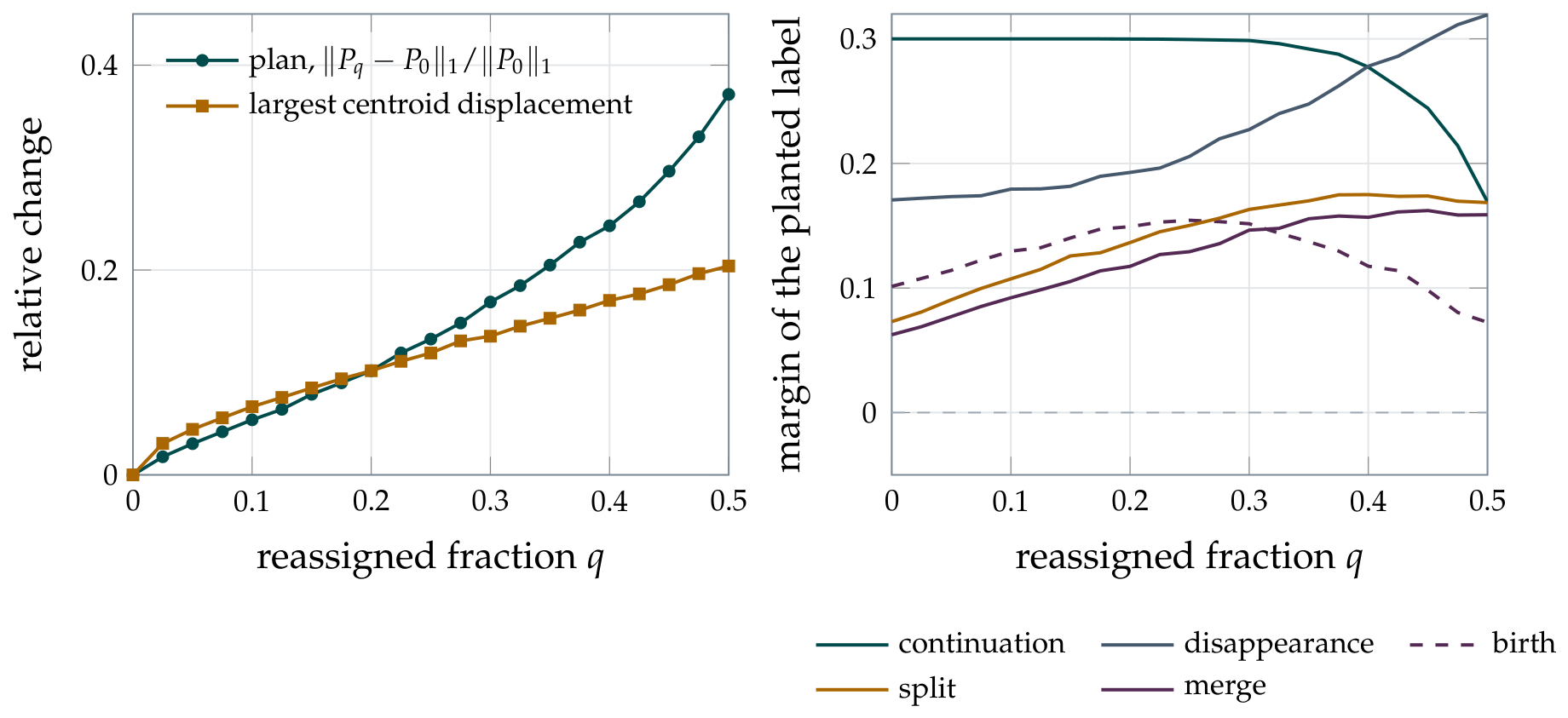
Appendix C.2. What the Figure Shows
The plan and the centroids move roughly linearly in q (the plan curves upward beyond ), as the first-order bounds say, with slopes far below the worst-case constants. The labels are far more robust than the plan: at , the plan has moved by and all five labels stand in every repetition, and the first losses appear at , when nearly half of every topic has been rewritten. The margins of the uneven split and merge grow, because reassignment across their own boundaries makes their shares more even; those of the continuation and the birth fall. A variant with random reassignment moves the plan more and erodes the split and merge margins from ; there they are the first labels lost ( and of repetitions at ). This is what Theorem 2 leads one to expect: a label survives while the decision error stays below half its margin, and a reassignment is far from the adversarial case the theorem allows for.
Appendix D. Two Further Notes
Appendix D.1. Overlapping Windows
When , a document can belong to both windows, and the same document then influences a source centroid and a target centroid. In the transport view, this is harmless to first order: an overlapping document perturbs the two centroids it touches by each, which by Lemma 2 perturbs the cost by and, by Theorem 1, the plan by . Overlap therefore contributes a term of the same order already present in Corollary 1, rather than a new source of error, which is the precise sense in which the soft plan is robust to the overlap that the system paper flagged as a concern.
Appendix D.2. Document-Level Transport
The topic-level plan uses centroid-to-centroid costs. A finer document-level version uses costs between a fixed document and the estimated target centroids. This is the level at which BERTilda’s hard outflow and inflow are most closely recovered: as and one marginal penalty is removed (with the reservoir column of Section 5.4), the soft document-to-topic plan approaches the nearest-centroid attribution used in the system. The stability transfer is therefore not an automatic identity between the topic-level and document-level plans; it is the same perturbation argument applied to a different cost matrix, under the analogous assumption that the only estimated landmarks in that matrix are the topic centroids.
References
- Oliveira, C.; Figueira, Á. BERTilda: Explainable Topic Lifecycle Tracking with Split/Merge Detection via Similarity-and-Flow Temporal Graphs. In Machine Learning and Knowledge Discovery in Databases. Research Track; Lecture Notes in Computer Science; Springer: Cham, Switzerland, 2026; Volume 16946, pp. 676–693. [Google Scholar] [CrossRef] [Scilit]
- Grootendorst, M. BERTopic: Neural Topic Modeling with a Class-Based TF-IDF Procedure. arXiv 2022, arXiv:2203.05794. [Google Scholar]
- Hofmann, T. Probabilistic Latent Semantic Analysis. In Proceedings of the Uncertainty in Artificial Intelligence (UAI), Stockholm, Sweden, 30 July–1 August 1999. [Google Scholar]
- Blei, D.M.; Ng, A.Y.; Jordan, M.I. Latent Dirichlet Allocation. J. Mach. Learn. Res. 2003, 3, 993–1022. [Google Scholar]
- Lee, D.D.; Seung, H.S. Learning the Parts of Objects by Non-Negative Matrix Factorization. Nature 1999, 401, 788–791. [Google Scholar] [CrossRef] [Scilit] [PubMed]
- Teh, Y.W.; Jordan, M.I.; Beal, M.J.; Blei, D.M. Hierarchical Dirichlet Processes. J. Am. Stat. Assoc. 2006, 101, 1566–1581. [Google Scholar] [CrossRef] [Scilit]
- Blei, D.M. Probabilistic Topic Models. Commun. ACM 2012, 55, 77–84. [Google Scholar] [CrossRef] [Scilit]
- Blei, D.M.; Lafferty, J.D. Dynamic Topic Models. In Proceedings of the International Conference on Machine Learning (ICML), Pittsburgh, PA, USA, 25–29 June 2006. [Google Scholar]
- Wang, X.; McCallum, A. Topics over Time: A Non-Markov Continuous-Time Model of Topical Trends. In Proceedings of the ACM SIGKDD International Conference on Knowledge Discovery and Data Mining (KDD), Philadelphia, PA, USA, 20–23 August 2006. [Google Scholar]
- Dieng, A.B.; Ruiz, F.J.R.; Blei, D.M. The Dynamic Embedded Topic Model. arXiv 2019, arXiv:1907.05545. [Google Scholar]
- Angelov, D. Top2Vec: Distributed Representations of Topics. arXiv 2020, arXiv:2008.09470. [Google Scholar]
- Dieng, A.B.; Ruiz, F.J.R.; Blei, D.M. Topic Modeling in Embedding Spaces. Trans. Assoc. Comput. Linguist. 2020, 8, 439–453. [Google Scholar] [CrossRef] [Scilit]
- Newman, D.; Lau, J.H.; Grieser, K.; Baldwin, T. Automatic Evaluation of Topic Coherence. In Proceedings of the Annual Conference of the North American Chapter of the Association for Computational Linguistics (NAACL-HLT), Los Angeles, CA, USA, 2–4 June 2010. [Google Scholar]
- Mimno, D.; Wallach, H.M.; Talley, E.; Leenders, M.; McCallum, A. Optimizing Semantic Coherence in Topic Models. In Proceedings of the Conference on Empirical Methods in Natural Language Processing (EMNLP), Edinburgh, UK, 27–31 July 2011. [Google Scholar]
- Röder, M.; Both, A.; Hinneburg, A. Exploring the Space of Topic Coherence Measures. In Proceedings of the ACM International Conference on Web Search and Data Mining (WSDM), Shanghai, China, 2–6 February 2015. [Google Scholar]
- Hoyle, A.; Goel, P.; Peskov, D.; Hian-Cheong, A.; Boyd-Graber, J.; Resnik, P. Is Automated Topic Model Evaluation Broken? The Incoherence of Coherence. In Proceedings of the Advances in Neural Information Processing Systems (NeurIPS), Virtual, 6–14 December 2021. [Google Scholar]
- Chakrabarti, D.; Kumar, R.; Tomkins, A. Evolutionary Clustering. In Proceedings of the ACM SIGKDD International Conference on Knowledge Discovery and Data Mining (KDD), Philadelphia, PA, USA, 20–23 August 2006. [Google Scholar]
- Spiliopoulou, M.; Ntoutsi, I.; Theodoridis, Y.; Schult, R. MONIC: Modeling and Monitoring Cluster Transitions. In Proceedings of the ACM SIGKDD International Conference on Knowledge Discovery and Data Mining (KDD), Philadelphia, PA, USA, 20–23 August 2006. [Google Scholar]
- Palla, G.; Barabási, A.L.; Vicsek, T. Quantifying Social Group Evolution. Nature 2007, 446, 664–667. [Google Scholar] [CrossRef] [Scilit] [PubMed]
- Greene, D.; Doyle, D.; Cunningham, P. Tracking the Evolution of Communities in Dynamic Social Networks. In Proceedings of the International Conference on Advances in Social Networks Analysis and Mining (ASONAM), Odense, Denmark, 9–11 August 2010. [Google Scholar]
- Rosvall, M.; Bergstrom, C.T. Mapping Change in Large Networks. PLoS ONE 2010, 5, e8694. [Google Scholar] [CrossRef] [Scilit] [PubMed]
- Kantorovich, L.V. On the Translocation of Masses. Dokl. Akad. Nauk. SSSR 1942, 37, 199–201, Reprinted in J. Math. Sci. 2006, 133, 1381–1382. [Google Scholar]
- Villani, C. Optimal Transport: Old and New; Springer: Berlin/Heidelberg, Germany, 2009. [Google Scholar]
- Peyré, G.; Cuturi, M. Computational Optimal Transport. Found. Trends Mach. Learn. 2019, 11, 355–607. [Google Scholar] [CrossRef] [Scilit]
- Sinkhorn, R. A Relationship Between Arbitrary Positive Matrices and Doubly Stochastic Matrices. Ann. Math. Stat. 1964, 35, 876–879. [Google Scholar] [CrossRef] [Scilit]
- Cuturi, M. Sinkhorn Distances: Lightspeed Computation of Optimal Transport. In Proceedings of the Advances in Neural Information Processing Systems (NeurIPS), Lake Tahoe, NV, USA, 5–8 December 2013. [Google Scholar]
- Chizat, L.; Peyré, G.; Schmitzer, B.; Vialard, F.X. Scaling Algorithms for Unbalanced Optimal Transport Problems. Math. Comput. 2018, 87, 2563–2609. [Google Scholar] [CrossRef] [Scilit]
- Liero, M.; Mielke, A.; Savaré, G. Optimal Entropy-Transport Problems and a New Hellinger–Kantorovich Distance Between Positive Measures. Invent. Math. 2018, 211, 969–1117. [Google Scholar] [CrossRef] [Scilit]
- Séjourné, T.; Feydy, J.; Vialard, F.X.; Trouvé, A.; Peyré, G. Sinkhorn Divergences for Unbalanced Optimal Transport. arXiv 2019, arXiv:1910.12958. [Google Scholar]
- Genevay, A.; Chizat, L.; Bach, F.; Cuturi, M.; Peyré, G. Sample Complexity of Sinkhorn Divergences. In Proceedings of the International Conference on Artificial Intelligence and Statistics (AISTATS), Okinawa, Japan, 16–18 April 2019. [Google Scholar]
- Kusner, M.J.; Sun, Y.; Kolkin, N.I.; Weinberger, K.Q. From Word Embeddings to Document Distances. In Proceedings of the International Conference on Machine Learning (ICML), Lille, France, 6–11 July 2015. [Google Scholar]
- Aurenhammer, F.; Hoffmann, F.; Aronov, B. Minkowski-Type Theorems and Least-Squares Clustering. Algorithmica 1998, 20, 61–76. [Google Scholar] [CrossRef] [Scilit]
- Hoeffding, W. Probability Inequalities for Sums of Bounded Random Variables. J. Am. Stat. Assoc. 1963, 58, 13–30. [Google Scholar] [CrossRef]
- McDiarmid, C. On the Method of Bounded Differences. In Surveys in Combinatorics; London Mathematical Society Lecture Note Series; Cambridge University Press: Cambridge, UK, 1989; Volume 141, pp. 148–188. [Google Scholar]
- Boucheron, S.; Lugosi, G.; Massart, P. Concentration Inequalities: A Nonasymptotic Theory of Independence; Oxford University Press: Oxford, UK, 2013. [Google Scholar]
- Le Cam, L. Convergence of Estimates Under Dimensionality Restrictions. Ann. Stat. 1973, 1, 38–53. [Google Scholar] [CrossRef] [Scilit]
- Yu, B. Assouad, Fano, and Le Cam. In Festschrift for Lucien Le Cam; Springer: New York, NY, USA, 1997; pp. 423–435. [Google Scholar]
- Tsybakov, A.B. Introduction to Nonparametric Estimation; Springer: New York, NY, USA, 2009. [Google Scholar]
- Campello, R.J.G.B.; Moulavi, D.; Sander, J. Density-Based Clustering Based on Hierarchical Density Estimates. In Proceedings of the Pacific-Asia Conference on Knowledge Discovery and Data Mining (PAKDD), Gold Coast, Australia, 14–17 April 2013. [Google Scholar]
- McInnes, L.; Healy, J.; Melville, J. UMAP: Uniform Manifold Approximation and Projection for Dimension Reduction. arXiv 2018, arXiv:1802.03426. [Google Scholar]
- Devlin, J.; Chang, M.W.; Lee, K.; Toutanova, K. BERT: Pre-Training of Deep Bidirectional Transformers for Language Understanding. In Proceedings of the Annual Conference of the North American Chapter of the Association for Computational Linguistics (NAACL-HLT), Minneapolis, MN, USA, 2–7 June 2019. [Google Scholar]
- Reimers, N.; Gurevych, I. Sentence-BERT: Sentence Embeddings Using Siamese BERT-Networks. In Proceedings of the Conference on Empirical Methods in Natural Language Processing (EMNLP-IJCNLP), Hong Kong, China, 3–7 November 2019. [Google Scholar]
- Wang, W.; Wei, F.; Dong, L.; Bao, H.; Yang, N.; Zhou, M. MiniLM: Deep Self-Attention Distillation for Task-Agnostic Compression of Pre-Trained Transformers. In Proceedings of the Advances in Neural Information Processing Systems (NeurIPS), Virtual, 6–12 December 2020. [Google Scholar]
- Kuhn, H.W. The Hungarian Method for the Assignment Problem. Nav. Res. Logist. Q. 1955, 2, 83–97. [Google Scholar] [CrossRef] [Scilit]
- Munkres, J. Algorithms for the Assignment and Transportation Problems. J. Soc. Ind. Appl. Math. 1957, 5, 32–38. [Google Scholar] [CrossRef] [Scilit]
- Birkhoff, G. Tres observaciones sobre el álgebra lineal. Univ. Nac. De Tucumán Rev. Ser. A 1946, 5, 147–151. [Google Scholar]
- Mémoli, F. Gromov–Wasserstein Distances and the Metric Approach to Object Matching. Found. Comput. Math. 2011, 11, 417–487. [Google Scholar] [CrossRef] [Scilit]
- Luise, G.; Rudi, A.; Pontil, M.; Ciliberto, C. Differential Properties of Sinkhorn Approximation for Learning with Wasserstein Distance. In Proceedings of the Advances in Neural Information Processing Systems (NeurIPS), Montréal, QC, Canada, 3–8 December 2018. [Google Scholar]
- Lange, T.; Roth, V.; Braun, M.L.; Buhmann, J.M. Stability-Based Validation of Clustering Solutions. Neural Comput. 2004, 16, 1299–1323. [Google Scholar] [CrossRef] [Scilit] [PubMed]
- Ben-David, S.; von Luxburg, U.; Pál, D. A Sober Look at Clustering Stability. In Proceedings of the Learning Theory (COLT 2006); Lecture Notes in Computer Science; Springer: Berlin/Heidelberg, Germany, 2006; Volume 4005, pp. 5–19. [Google Scholar]
- von Luxburg, U. Clustering Stability: An Overview. Found. Trends Mach. Learn. 2010, 2, 235–274. [Google Scholar] [CrossRef] [Scilit]
- Strehl, A.; Ghosh, J. Cluster Ensembles: A Knowledge Reuse Framework for Combining Multiple Partitions. J. Mach. Learn. Res. 2002, 3, 583–617. [Google Scholar]
- Monti, S.; Tamayo, P.; Mesirov, J.; Golub, T. Consensus Clustering: A Resampling-Based Method for Class Discovery and Visualization of Gene Expression Microarray Data. Mach. Learn. 2003, 52, 91–118. [Google Scholar] [CrossRef] [Scilit]
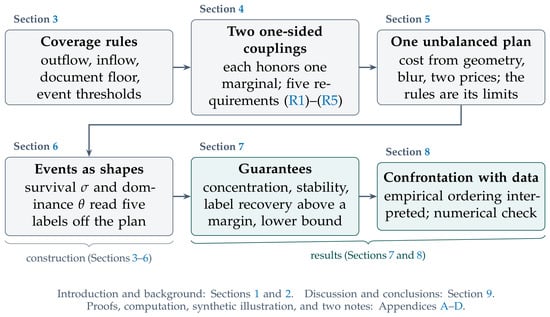
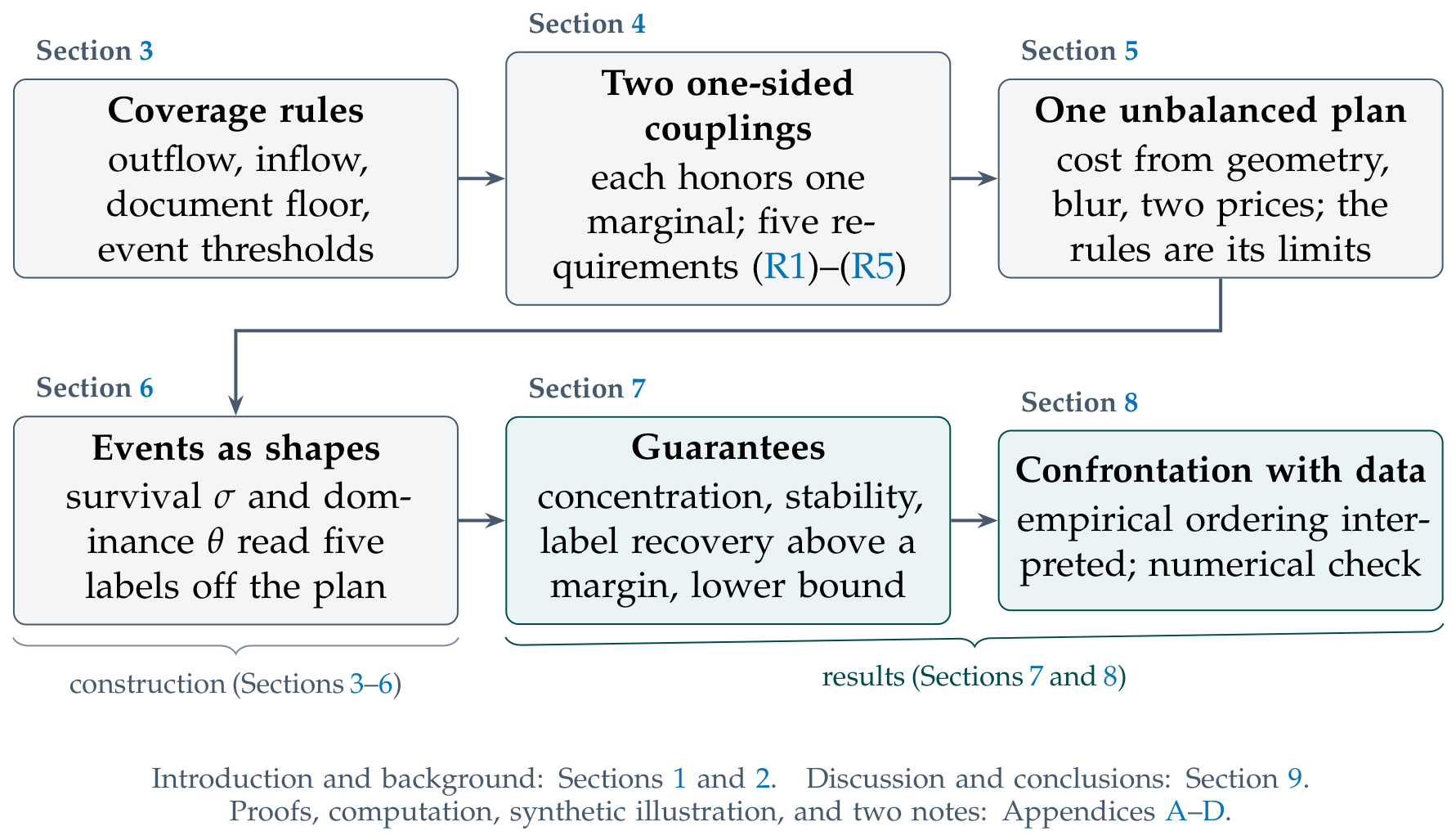
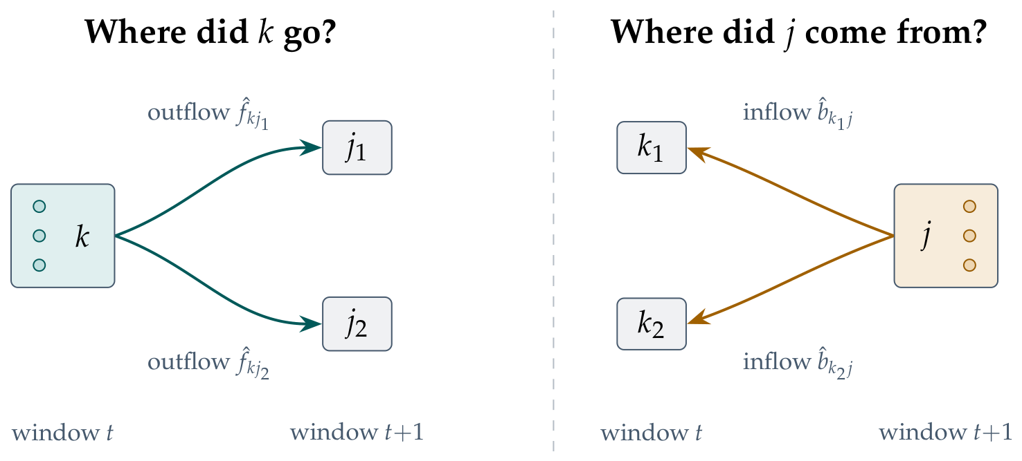
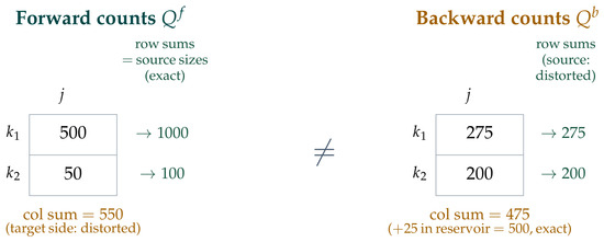
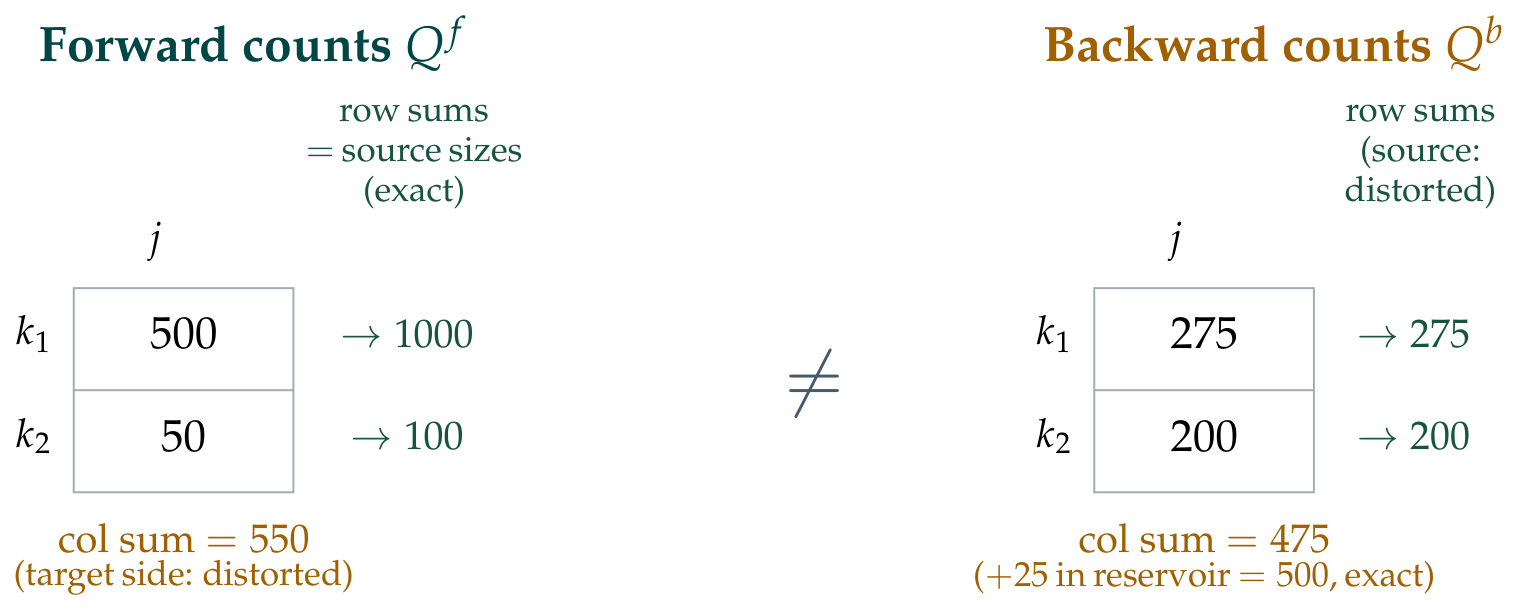
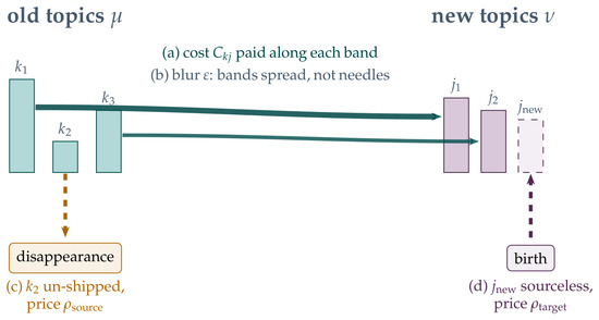
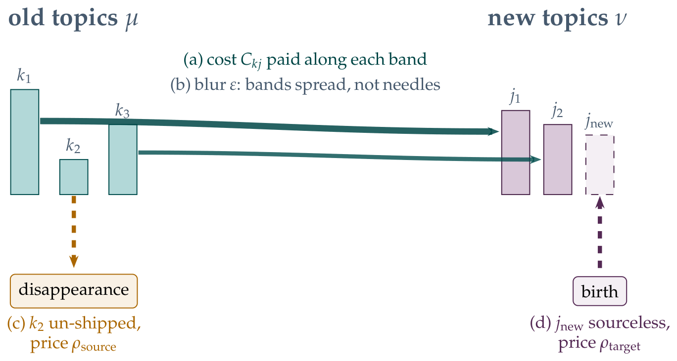
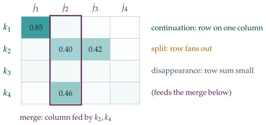
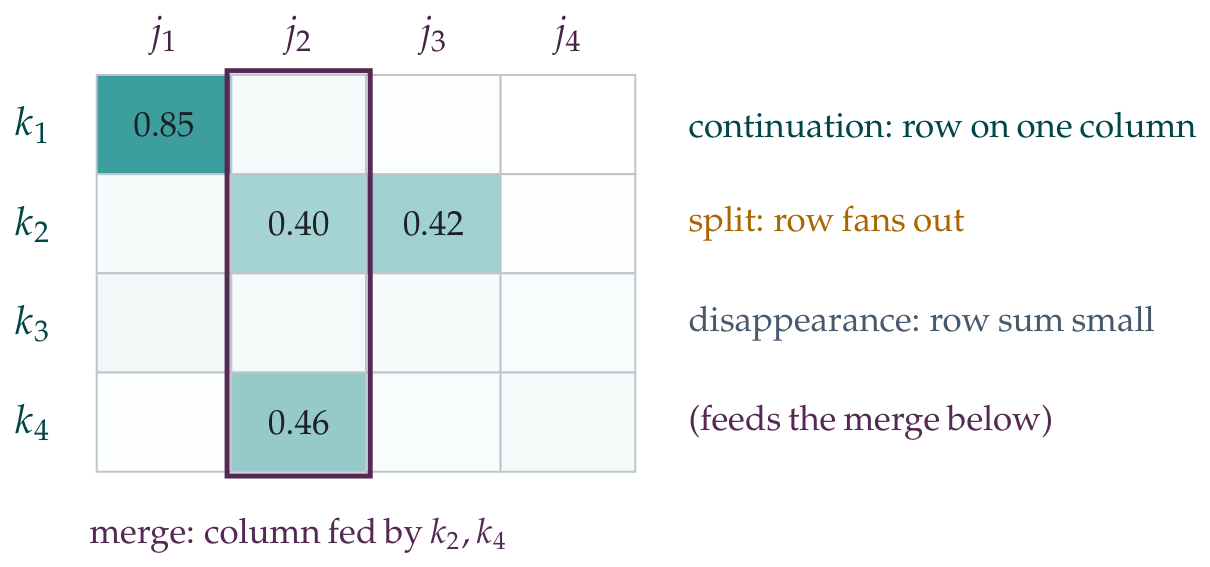
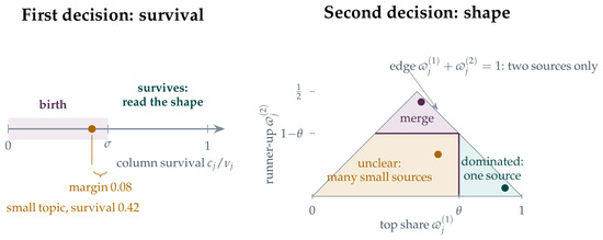
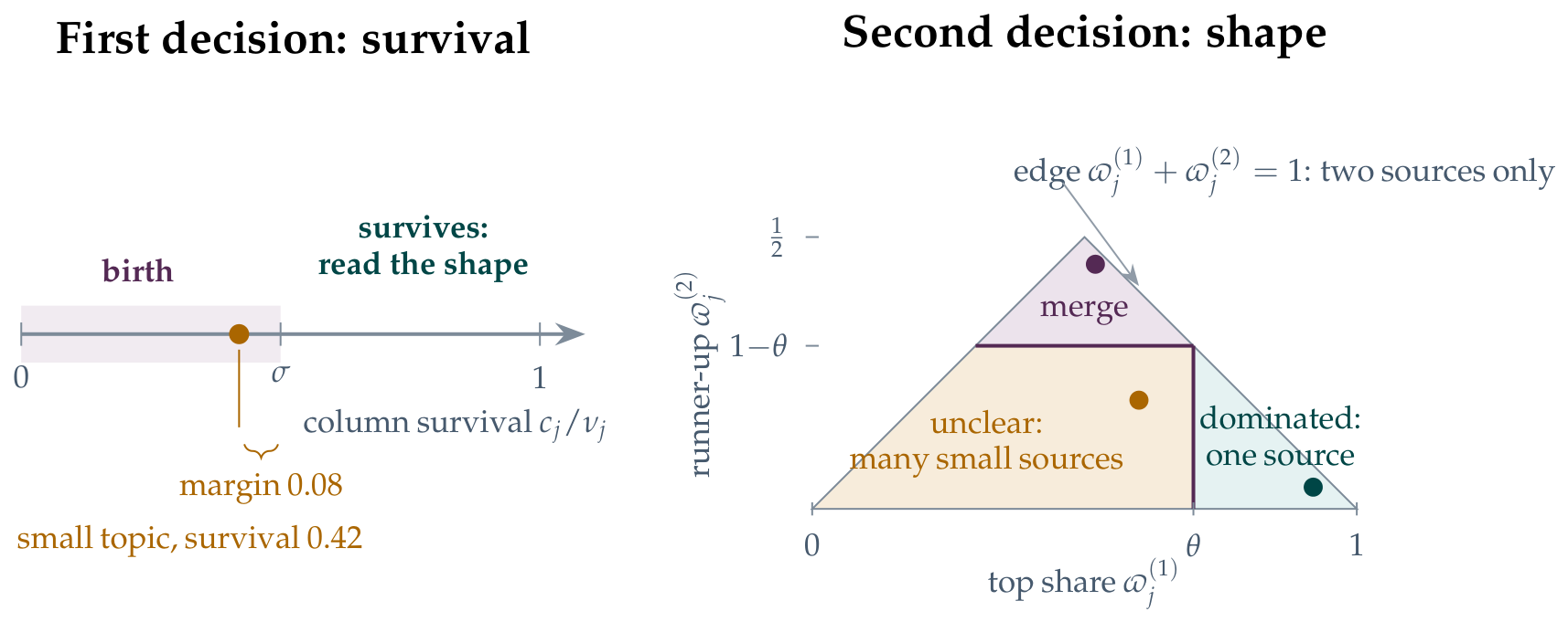
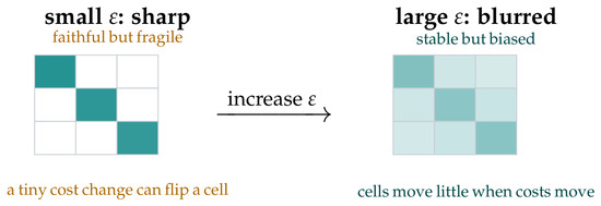
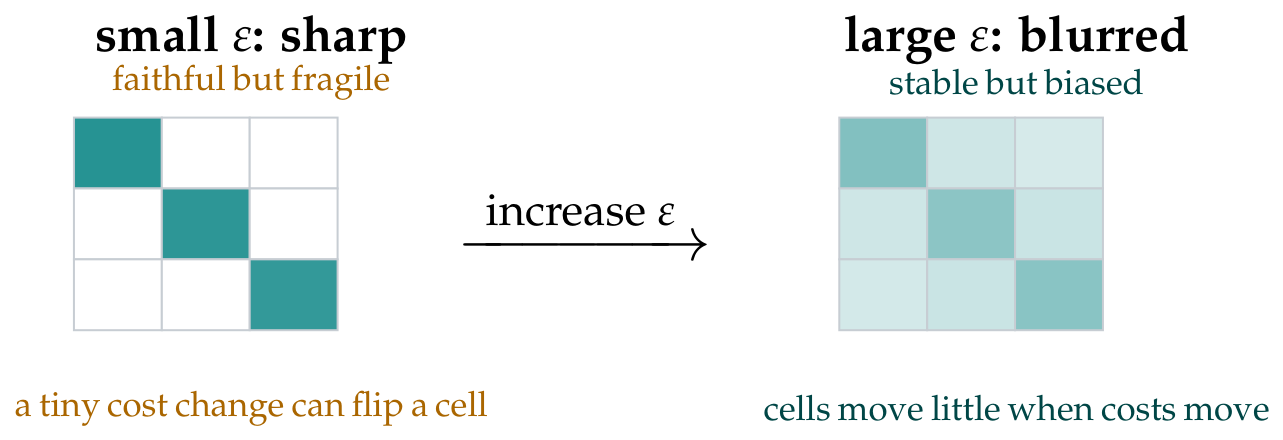
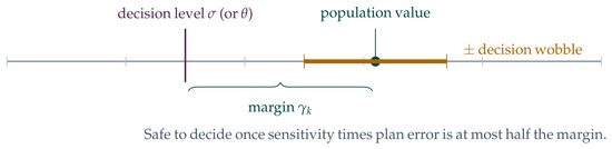
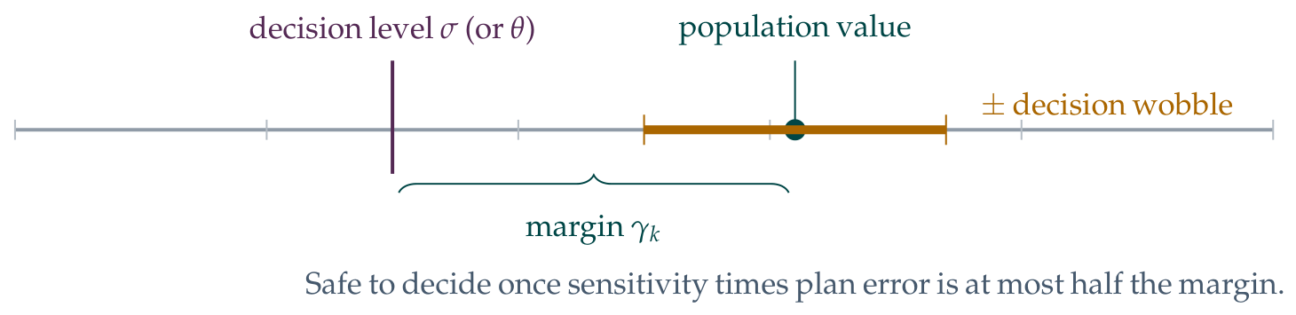
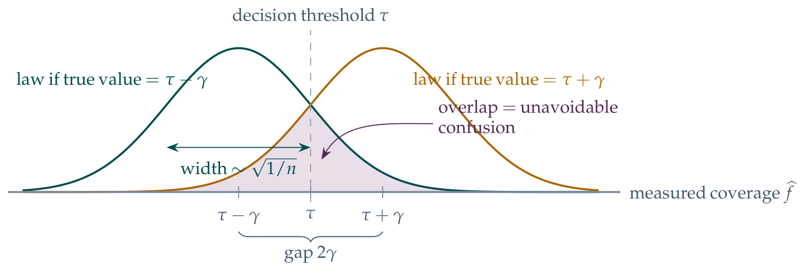

Disclaimer/Publisher’s Note: The statements, opinions and data contained in all publications are solely those of the individual author(s) and contributor(s) and not of MDPI and/or the editor(s). MDPI and/or the editor(s) disclaim responsibility for any injury to people or property resulting from any ideas, methods, instructions or products referred to in the content. |
© 2026 by the authors. Licensee MDPI, Basel, Switzerland. This article is an open access article distributed under the terms and conditions of the Creative Commons Attribution (CC BY) license.