


Abstract
An exact projective compactification is established and implemented for quoted-band superhedging of activated Bitcoin calls with payoff . The computation is exact on the terminal half-line, conditional on a disclosed finite first-date support; no equality with a continuum of first-date states is claimed. Recession variables are identified as projective-boundary atoms, one per first-date source node, and the finite-knot inequalities with the terminal-slope rows are proved necessary as well as sufficient for the semi-infinite continuous-terminal hedge. Only quoted bid–ask bands are used: no fitted volatility surface, no mid-price substitution, and no ex post quote repair. Across 82 monthly Deribit snapshots from October 2019 to July 2026 and two maturity pairs, 161 of 164 panels are feasible. Median reductions from the constant-delta value, conditional on the disclosed finite first-date support throughout, are 6.35% for 1M/2M and 3.30% for 3M/6M, against a median relative interval width of 42.65%, so these are seller-capital savings rather than point estimates of market value. Deleting the recession rows changes no feasible value measurably, yet at the smallest terminal cutoff, it creates 125 false infeasibility classifications and 431 hedges that pass every finite-grid test while failing the omitted terminal ray. Price stability and certificate validity are, therefore, distinct properties.
Keywords:
martingale optimal transport; robust superhedging; bid–ask spreads; Bitcoin options; barrier options; linear programming; quoted-band calibration; model risk MSC:
91G20; 91G80; 90C05; 60E15
1. Introduction
Market prices provide a finite collection of imperfect option quotes, not an exact continuous risk-neutral distribution. Consequently, a path-dependent or multi-date claim is generally only partially identified. Model-independent pricing replaces a selected stochastic model with an optimization over all laws compatible with observed instruments and the relevant no-arbitrage restrictions. In the two-date setting, the resulting martingale optimal transport (MOT) problem connects a primal optimization over couplings to a semi-static superhedging problem [1,2,3,4,5].
A two-date activated call written on forward-normalized Bitcoin prices is studied:
Activation is monitored only at , and the call payoff is delivered at . The claim combines a discontinuity in the first coordinate with unbounded linear growth in the second. It therefore exposes two numerical choices that can otherwise remain hidden, namely, whether equality at the threshold activates the contract and whether a finite terminal truncation has been supplemented by a valid asymptotic-slope condition.
The empirical question is the value of conditional information in the inter-maturity hedge. A conditional-martingale formulation, whose dual permits the node-specific inter-maturity delta at source node after observing the first-date state, is compared with a relaxation that permits only one common inter-maturity . For a disclosed finite grid , define
whenever . Here, and are exact values of the projectively compactified continuous-terminal problem conditional on the disclosed finite support. No equality with, or approximation bound for, a model having continuous support is asserted. Equality with ordinary finite-first-moment laws is governed by the density and attainment conditions in Theorem 1.
The empirical design uses 82 first-of-month Deribit option-chain snapshots from October 2019 through July 2026. Each month contributes a 1M/2M and a 3M/6M maturity pair. The principal specification holds the normalized contract fixed at and uses the closed-touch event . Vanilla prices are required to lie in finite bid–ask bands. A symmetric numerical pad of is fixed before solving; quote bands are not widened case by case. Incompatible quote boxes remain in the sample ledger, and no claim value is reported for them.
The contribution is deliberately contract-specific. General pricing–hedging duality and computational MOT are established [1,2,3,4,5], and the more specialized antecedents in robust barrier hedging, finite-quote consistency, bid–ask MOT, and cryptocurrency option markets are reviewed in Section 2. Beyond the application of finite LP duality, three further results are established. The recession columns are identified as atoms at the projective boundary. The finite program is proved to be an exact reduction of the continuous-terminal generalized-moment problem. The finite-knot inequalities together with the terminal-slope rows are shown to be necessary and sufficient for semi-infinite terminal super-replication at every disclosed first-date node. The empirical contribution is an auditable activated-call implementation with a long two-maturity Bitcoin panel, explicit closed-versus-strict threshold treatment, quote-box infeasibility reporting, full-panel recession ablation, and grid and market-convention robustness checks.
The main findings are as follows. Of 164 quote-only panels, 161 are feasible. The median relative reduction from the constant-delta to the conditional upper value, conditional on the disclosed finite first-date support throughout, is 6.35% for 1M/2M and 3.30% for 3M/6M. Across 79 months feasible for both maturity pairs, the median difference is 3.04 percentage points, and the short-pair reduction is larger in 93.67% of cases. Median absolute reductions, however, are 0.004980 and 0.005233, respectively, so the larger relative percentage for 1M/2M does not imply a larger absolute saving. An exact-mean companion leaves 158 panels feasible and produces comparable medians on its feasible subset. Full-panel source-grid refinements, an independent common-grid audit, and a global 80-fill-node grid preserve every status and the headline medians. Targeted maturity windows preserve the short-versus-long ordering. Quote-age removal affects few panels and leaves feasibility unchanged, whereas positive- conventions materially shrink the quote-box feasible set and must therefore be reported jointly with common-feasible value comparisons. Every feasible main case passes finite-cell and terminal-ray hedge tests at tolerance .
The remainder of the article is organized as follows. The study is positioned in the literature in Section 2. The ambiguity sets, finite programs, and analytical properties are defined in Section 3. The data and computational design are described in Section 4. The main panel and sensitivity results are reported in Section 5. Mechanisms, economic implementation, limitations, and decision rules are discussed in Section 6. Conclusions are drawn in Section 7.
2. Related Literature and Positioning
Model-independent option bounds can be formulated as transport problems constrained by observed option prices. Beiglböck et al. [1] established the mass-transport approach to option-price bounds, Acciaio et al. [2] developed model-free asset-pricing and super-replication results, and Dolinsky and Soner [3] treated continuous-time robust hedging. Complete one-dimensional MOT duality and computational methods are developed in [4,5]. Structural solution theory includes the left-curtain coupling [6], a stochastic-control construction for marginally constrained bounds [7], and an explicit martingale analogue of the one-dimensional Brenier theorem [8]. These results explain how dependence restrictions, rather than marginal option information alone, determine path-dependent values.
Static-arbitrage consistency of finitely traded option prices is therefore central [9]. Barrier claims are direct antecedents because activation makes the payoff sensitive to threshold events. Brown et al. [10] and Cox and Obłój [11] derive robust barrier hedges, while forward-start bounds in [12,13] illustrate how intermediate-state information changes robust values. Robust pricing–hedging duality has also been extended to continuous-time, nondominated discrete-time, and pointwise model-free frameworks [14,15,16]. The value of enlarging the information set in pricing and hedging is formalized in [17], although the present comparison is specifically between state-dependent and constant inter-maturity deltas.
Finite option menus require a separate consistency layer. Sufficient no-arbitrage conditions, exact calibration restrictions, and algorithms for detecting and repairing static arbitrage are studied in [18,19,20]. Bid–ask consistency is characterized in [21], while convex optimization over option-implied distributions and risk-neutral probabilities is developed in [22,23]. In this study, those ideas are used only diagnostically, as the pre-specified quote bands are never repaired or widened after observing feasibility, and incompatible panels remain in the sample ledger.
Recent work further narrows the distance to the present setting. Liang et al. [24] formulate bid–ask MOT, establish strong duality, and give a multi-maturity interpretation with state-dependent delta. Dynamic option trading and intermediate marginals are analyzed in [25,26], and structured multimarginal computation in [27]. Chen et al. [28] empirically evaluate model-free valuation and hedging for equities. Zhuang [29] is the closest single antecedent and is therefore separated out. That study also works from finite two-sided quotes, also reduces the problem to a finite linear program, also carries an explicit variable for mass at a threshold, and also establishes sharpness of the resulting set on a large multi-year weekly SPX panel. Three differences are material here. The threshold there is a terminal crash event and the object characterized is a two-dimensional identified set of probability and conditional depth, whereas the threshold here is a first-date activation event and the object is a one-dimensional upper value for a two-date claim. The unbounded linear recession direction in the terminal coordinate does not arise there and is what requires the compactification used below. No comparison between state-dependent and constant inter-maturity rebalancing is available in that setting, because it has one maturity. Lee [30] studies multi-maturity consistency under bounded bid–ask spreads and constructs an exact two-date basket operator. Its Proposition 5.3 bears directly on the present argument: an infimum over an unbounded terminal half-line is evaluated at the terminal strikes whenever the candidate slope is bounded below by the asymptotic slope of the terminal payoff, which is the scalar form of the reduction used below. Two differences separate that result from Corollary 1. Proposition 5.3 evaluates one payoff against one asymptotic slope, whereas Corollary 1 establishes that a finite row system is necessary as well as sufficient for the semi-infinite continuous-terminal hedge. The bounded-spread two-date setting carries no first-date event on which tail behavior can depend, so no counterpart of the source-dependent recession columns arises there. Thus, strong duality, adaptive delta, threshold mass, quote-band consistency, and finite-knot evaluation on a half-line are prior art rather than contributions of this study.
The incremental positioning is made explicit in Table 1.
Table 1.
Positioning relative to the closest methodological and empirical antecedents.
Bitcoin option research has mainly followed parametric or semiparametric routes. Advanced calibration, cryptocurrency-option pricing, regime-switching GARCH, stochastic-volatility, jump, and liquidity specifications are developed in [31,32,33,34,35,36,37]. This literature demonstrates that model choice is consequential for Bitcoin option values. In this study, the joint law is instead deliberately left partially identified by the quoted-band program.
Option-implied Bitcoin information is also used to forecast volatility and recover expected-return term structures [38,39]. Trade direction and net buying pressure carry information [40], while aggregate illiquidity is associated with crypto-option returns [41]. These findings motivate caution when interpreting top-of-book bands as executable capacity: the LP uses price endpoints, but depth, order size, and market impact are not modeled.
Finally, Bitcoin returns exhibit jumps in both lower-frequency and high-frequency analyses [42,43], and Bitcoin option-implied volatility slopes are linked to jumps [44]. Such tail behavior strengthens the case for an explicit terminal-growth certificate rather than an unqualified finite truncation. Mathematically, the quote inequalities are linear moment restrictions of the type studied in transport with additional linear constraints [45], and the finite primal–dual equality used below is standard convex/linear-programming duality [46].
In the present study, the setting departs from the classical exact-marginal formulation in two respects. First, the observations are finite bid–ask intervals rather than exact call curves. Second, the payoff is discontinuous in and has an unbounded linear recession direction in . Both affect closure, feasibility, and numerical certification. Accordingly, no new general MOT duality, new general threshold method, continuous- exact representation, or bibliographic priority is claimed in this paper. The projective device itself is the standard homogenization used for moment problems with linear growth on non-compact supports, and no priority is claimed for it. What is established here is its exact finite-knot consequence for this constraint system, together with the corresponding certificate. Its novelty lies in the proved continuous- projective compactification conditional on finite first-date support and in the conjunction of a two-date activated-call contract, a long cryptocurrency-options panel, a fixed quoted-band convention without data-dependent repair, closed-threshold disclosure, full recession/grid/market ablations, and independently assembled primal–dual terminal-ray certificates.
3. Model and Analytical Results
3.1. Contract and Quoted-Band Ambiguity Sets
The notation used throughout is collected in Table A1; the compactified and financial programs share it. The benchmark supremum over laws with continuous support in both coordinates is easily conflated with the value on the disclosed finite first-date grid. The two are not identified, and no approximation bound between them is claimed.
For each retained vanilla option , let denote its normalized payoff and its retained lower and upper quote endpoints. A candidate law must satisfy
These are additional linear moment constraints in the sense of constrained optimal transport [45]. No smooth implied-volatility surface is fitted, and mid prices do not replace two-sided quotes. In the dual, a long option position is charged at the padded upper endpoint, and a short position is credited at the padded lower endpoint. This is a quoted-band valuation convention. It does not assert unlimited execution at top-of-book quantities.
Let be the set of probability measures on with finite first moments that satisfy all quoted-band constraints and
Let impose only
and let impose no inter-maturity martingale restriction. Then,
The aggregate condition is not an alternative martingale model, as one unconditional mean-increment equality does not imply the conditional martingale property. It is the primal representation of the constant-delta relaxation and is used only to measure the value of state-dependent rebalancing.
The continuous-state benchmark values are
The empirical quantities reported below are finite-source values . Theorem 1 identifies them exactly with the projectively compactified continuous- problem conditional on the disclosed support. It does not identify them with the benchmarks having continuous support.
3.2. Semi-Static Dual Strategies
For the conditional model, let denote the inter-maturity delta at source node . The dual hedge takes the form
where . Its quoted-band cost is
For a continuous-state superhedge, one would require for all . This inequality is verified by the implementation for each selected source node and all , as established in Corollary 1 below. Verification remains nodewise on the disclosed grid. Because restricting the first-date support shrinks the set of admissible laws, the reported value is no larger than its continuum-support counterpart. The finite-source bound understates the model-free superhedging cost rather than overstating it, and the certificate is a statement about the disclosed nodes rather than about every first-date state. In the aggregate model, is replaced by one constant delta. Vanilla positions remain static. Only the forward/delta leg can be adjusted after is observed. No separate dynamic position is included in the baseline formulation from time 0 to .
A useful comparator is the terminal call:
If strike is listed and retained, its padded upper quote endpoint is a finite-state upper bound. If is not listed, any retained terminal call with strike remains valid because . Cash alone cannot superhedge the claim on an unbounded terminal state because the payoff grows linearly as .
3.3. Compactified Finite-State Primal Program
Let contain all retained strikes, the structural nodes 0 and 1, the contract points and , interior fill nodes, and geometric tail nodes. The variable represents mass at . The variable is a recession first-moment variable for probability moving to conditional on source node . Its limiting probability mass is zero, but its limiting first moment can be nonzero.
The total-mass constraint is
The conditional martingale rows are
For the constant-delta relaxation, these equations are replaced by
For a option,
For a put,
whereas the terminal call includes the recession moment with unit slope:
The finite-state objective is
Let be the polyhedron determined by mass, quote, recession, and conditional or aggregate restrictions and
Theorem 1 proves that this formulation treats the entire terminal half-line exactly in the linear-growth closure conditional on the finite support. It does not remove the discretization. Equality with ordinary laws is governed by the density and attainment conditions stated in the theorem.
3.4. Direct Finite-Dimensional Dual
Let . For every finite cell, the conditional dual imposes
For each source node , the terminal ray imposes
where is the set of retained calls. Terminal puts and options have zero positive- tail slope. The objective is
In the aggregate comparator, all are replaced by one . For the numerical cross-check, this dual is assembled directly from the financial inequalities rather than by transposing the stored primal matrix or reusing primal solver multipliers.
3.5. Exact Projective Compactification and Continuous-Terminal Equivalence
The computation is exact on the terminal half-line, conditional on a disclosed finite first-date support. No equality with a continuum of first-date states is claimed, and the direction of that restriction is stated in Section 6.6.
The meaning of the recession variables and the continuous problem that is solved exactly are specified in this subsection. The first-date state remains restricted to the disclosed finite support
whereas the terminal state ranges over the full half-line . Let denote retained normalized vanilla payoffs when , and put
The four conditions are imposed and tailored with the traded menu.
(A1) The first-date support is finite.
(A2) Every , , and is continuous and piecewise affine, all finite kinks belong to one set , and every function is affine on . Its recession slope is denoted by
Thus, options and puts have zero recession slope, and calls have unit slope.
(A3) The terminal grid contains every and has ; non-kink fill and tail nodes are allowed.
(A4) Each quote constraint is a finite closed band , the compactified feasible set below is nonempty, and the conditional or aggregate mean-increment equality is exact.
An additional equality with payoff independent of , such as , is also admissible.
For nonnegative finite Borel measures on with finite first moment, let be the ordinary continuous-terminal upper value subject to the explicit total-mass equation , the quote bands, any stated -independent equality, and either
in the conditional regime, or
in the aggregate regime. To close the linear-growth direction, introduce the projective coordinate
and, for every relevant payoff , the continuous extension
The lift of an ordinary law is the finite measure on defined by
An atom is boundary mass in the weighted projective measure. It contributes no probability mass in the original scale because the transformed mass payoff is , but it contributes to every linear recession direction and is, therefore, a recession first moment in the original scale. Let be the upper value after such boundary atoms are admitted while all transformed constraints are retained.
Theorem 1
(exact projective compactification, finite reduction, and semi-infinite duality). Under (A1)–(A4), for define
Impose , the quote bands , the optional equality when present, and, respectively,
or
Let be the maximum of over this finite-dimensional feasible set. Then,
- The compactified continuous-terminal problem has the exact finite representationConsequently, is boundary mass in the weighted projective measure, equivalently a recession first moment in the original scale, not an ad hoc truncation correction.
- 2.
- The finite-dimensional feasible set is compact, and a nonempty problem has a finite attained maximum. In both regimes,
- 3.
- For a conditional hedgewith a common replacing the in the aggregate regime, the constraints for every and are equivalent to the finite-grid inequalities below (the rows at non-kink fill nodes are redundant):and the terminal-slope inequalitiesFor the present activated call, Equation (37) is
- 4.
- The cash variable and the dynamic multipliers (or the common aggregate multiplier ) are unrestricted real numbers. Let be the infimum ofover hedges satisfying the semi-infinite inequalities. If an additional -independent equality is imposed, introduce an unrestricted multiplier , replace by , and add to Equation (39). For the exact-mean companion, and . The infimum is attained, and
- 5.
- For ordinary probability laws,Equality holds whenever ordinary feasible laws are dense in the compactified feasible set for the finite family of moments used here. A concrete sufficient condition is that every quote band has positive width and there exists a compactified feasible point that satisfies every quote inequality strictly and has for every source . A separate sufficient condition for the compactified maximum itself to be attained by an ordinary law is that an optimizer has for all , or that every row with also has positive finite mass at a node in the common affine tail.
Proof.
If on an interval, Equation (28) gives , which is affine in . Hence, every transformed quote payoff, dynamic increment, target payoff, and the transformed mass payoff is affine between consecutive points and on .
For a finite measure on any interval , replace its restriction by endpoint masses
This preserves the integral of every affine function. Applying the replacement on every transformed grid interval, with a disjoint half-open convention at shared endpoints, gives, for each , an atomic measure supported on and simultaneously preserves mass, every quote moment, the applicable dynamic equations, and the objective. Thus, the intervalwise compression is exact. If is the mass of at , set
Conversely,
maps every nonnegative back to a compactified atomic measure with the same moments. This value-preserving correspondence proves Equation (33).
Equation (34) follows by adding either the conditional Equation (31) or the aggregate Equation (32) and using unit mass. Therefore and . The finite-dimensional feasible set is closed and bounded; the linear-growth target is bounded there. Weierstrass’ theorem yields primal attainment.
For a hedge Equation (35), define the transformed residual
It extends continuously to , where
The residual is affine on each transformed grid interval. Nonnegativity on is equivalent to nonnegativity at every interval endpoint. At finite endpoints, its sign is the sign of ; at , nonnegativity is exactly Equation (37). This proves the finite-knot equivalence.
After this reduction, the compactified primal and quoted-band dual are finite linear programs. Primal feasibility and Equation (34) give a finite attained primal optimum. Standard finite-dimensional LP strong duality [46] gives an attained dual optimum with cost Equation (39), including the term when the optional equality is present. Since Equations (36) and (37) are equivalent to the semi-infinite hedge inequalities, that finite dual is exactly , proving Equation (40). The optional term is an ordinary finite-dimensional equality multiplier and does not affect the reduction.
Every ordinary law lifts through Equation (29) to a compactified law without boundary mass, proving Equation (41). For the sufficient density condition, let be a compactified optimizer and set , . All quote moments of are strictly interior, and every source row has strictly positive finite-node mass. For each with , choose with , remove from that node, put it at
and set the corresponding recession variable to zero. Row mass and the required first moment are preserved exactly. Once , the change in any other moment relative to its compactified value is
which tends to zero with ; the same holds for the target. Strict quote slack therefore permits an ordinary feasible law whose value is arbitrarily close to . Sending first and then proves equality in Equation (41). If the donor lies in the common affine tail, the bracket in Equation (48) is identically zero, so the construction preserves all moments and the objective exactly and proves the stated ordinary-law attainment condition. □
Corollary 1
(necessary and sufficient terminal hedge certificate). Under (A1)–(A3), a recovered hedge super-replicates the activated call for every at every disclosed source node if and only if it satisfies all finite-grid inequalities Equation (36)—equivalently, the knot rows, since non-kink rows are redundant—and all terminal-slope inequalities Equation (38).
Proof.
Sufficiency is part 3 of Theorem 1. Necessity follows by evaluating the pathwise inequality at the finite grid nodes (in particular, the knots) and by dividing it by and letting . □
Lemma 1
(lower finite-knot and recession certificate). Under (A1)–(A4), let be the finite-dimensional feasible set in Theorem 1, for , and define the compactified lower value by
Let denote the infimum of the same target over the compactified continuous-terminal feasible measures. Then, the minimum in Equation (49) is finite and attained, and
For nonnegative static quantities , set and consider the conditional subhedge
with a common replacing in the aggregate regime. The semi-infinite inequalities for every and are equivalent to
together with the reversed terminal-slope inequalities
The row at and the rows at all finite kinks suffice in Equation (52); non-kink fill and tail-node rows are redundant. For the activated call, Equation (53) becomes
because options and terminal puts have zero recession slope, whereas terminal calls have unit recession slope.
Define the liquidation value of the subhedge by
Thus, a long static position is valued at the bid and a short static position at the ask. If the optional equality is imposed, add an unrestricted term to Equation (51) and to Equation (55). Let be the maximum of Equation (55) over the subhedges satisfying Equations (52) and (53). Then, this maximum is attained and
If denotes the infimum over ordinary feasible laws, then
Equality in Equation (57) follows under the same density condition stated in part 5 of Theorem 1. Accordingly, without that additional condition, is an exact interval for the projective closure and an outer interval for values generated by ordinary feasible laws.
Proof.
The intervalwise projective compression in the proof of Theorem 1 preserves every constraint and the target moment . The argument is value preserving and does not depend on whether that target is maximized or minimized. It therefore maps the compactified continuous-terminal minimization exactly onto Equation (49). The compactness established in part 2 of Theorem 1 then gives finiteness and attainment of the minimum, proving Equation (50).
It remains to establish the pathwise lower certificate and its finite-LP relation. Beyond the largest finite kink, every retained payoff is affine. Hence, at a fixed source node ,
If for all , division by and passage to the limit yield Equation (53). This is why the lower-side terminal inequality is reversed relative to the superhedge inequality. For sufficiency, put and define
The function is affine between consecutive transformed knots and extends continuously to , where
Conditions Equations (52) and (53) are exactly nonnegativity of this residual at all interval endpoints, including the projective boundary. Affinity therefore gives throughout , which is equivalent to for all finite . This also proves that non-kink fill and tail-node rows are redundant and establishes the activated-call specialization Equation (54).
Finally, write each band as the two inequalities:
In the dual of the finite minimization problem Equation (49), the multipliers of these two upper-bound-form rows are nonpositive. Write them as and , respectively, with . The resulting static coefficient is
and the corresponding contribution to the dual objective is
The unrestricted multipliers of the mass and martingale equalities are and (or the common ). The dual constraint associated with each is Equation (52), while the constraint associated with is Equation (53). An optional -independent equality contributes the unrestricted multiplier , has zero terminal slope, and changes the objective by . Standard finite-dimensional LP strong duality and dual attainment now give Equation (56). This is the ordinary dual of the finite program obtained after the exact projective reduction; it is not a new general MOT duality theorem. Since every ordinary feasible law lifts to a compactified feasible law, Equation (57) follows; density gives the stated equality. □
Corollary 2
(terminal-grid invariance). Under (A1)–(A4), hold and the quoted-band constraint system fixed. Replacing by any other terminal grid satisfying (A3), including by adding or removing non-kink fill nodes, does not change in exact arithmetic, provided the recession variables are retained.
Proof.
Every terminal grid satisfying (A3) represents the same compactified problem by Equation (33). □
Corollary 2 concerns only terminal-coordinate refinement; simultaneous refinement in and changes both the admissible first-coordinate support and the available state-dependent deltas. Theorem 1 identifies recession columns as projective boundary atoms, proves exact continuous- finite-knot reduction, and distinguishes the attained compactified optimum from the ordinary-law supremum. It is not presented as a new general MOT duality theorem. Nothing in the proof uses the activated-call form of the payoff, i.e., only (A2) is required, so the statement holds verbatim for any finite family of continuous piecewise-affine payoffs with a common finite kink set and affine tails. The activated call is retained as the running example because it is the contract studied empirically below.
No priority is claimed for the standard components of Theorem 1. The projective device itself is the classical homogenization used for moment problems with linear growth on non-compact supports [45,46]. It reparametrizes the terminal half-line so that linear-growth payoffs extend continuously to a compact space and escaping mass appears as boundary atoms. Strong duality and dual attainment for the finite program in part 4 are ordinary finite-dimensional linear programming, as the derivation preceding Equation (56) already states. One-dimensional convex analysis supplies the rest, since a continuous piecewise-affine function with finitely many kinks and an affine tail is dominated on a half-line exactly when it is dominated at its kinks and in the limiting slope. The same scalar reduction appears in [30], Proposition 5.3 (Finite evaluation), where an infimum over an unbounded terminal half-line collapses to the terminal strikes once the candidate slope is bounded below by the asymptotic slope of the payoff. Corollary 1 operates on the constraint system rather than on a single payoff, establishing that the finite-knot rows together with the terminal-slope rows are necessary as well as sufficient, with one recession column per first-date source node.
What the theorem adds is the consequence of combining them on this constraint system. The recession columns are identified, where ui is the boundary mass of the weighted projective measure, equivalently, a recession first moment. The recession payoff is source-dependent because activation is resolved at the first date, so each source node carries its own boundary column rather than one shared column. The reduction is exact and not approximate, and it is an equivalence and not an implication. Corollary 1 shows that the finite knot rows together with the terminal-slope rows are necessary as well as sufficient. A recovered hedge is therefore certified completely by finitely many inequalities, with nothing left outside the check. Corollary 2 follows immediately. The attained compactified optimum is separated from the ordinary-law supremum, with the density and attainment conditions under which they coincide stated and not assumed.
Everything downstream is empirical implementation, covering the quoted-band panel construction, the recovered-hedge certification, the recession ablation and the infeasibility diagnostics, none of which extends the theorem. The ablation of Section 5.9 is nevertheless what gives the theorem force. Omitting the recession rows leaves every feasible value unchanged, yet produces 125 false infeasibility classifications and 431 hedges that pass every finite-grid test and fail the omitted ray.
3.6. Analytical Properties
The following results distinguish general ordering properties from empirical regularities. In Propositions 1–3 and 5, is a placeholder, not a third value. Each statement applies separately to either the continuous benchmark or the finite-source value under one fixed, nonempty constraint system. These propositions do not identify the finite model with the continuous- benchmark.
Proposition 1 (Nesting and terminal-call upper bound).
If the relevant sets are nonempty, then
If a call at strike belongs to the same quote system with upper endpoint , then . If is unlisted, every retained call with gives the conservative bound .
Proof.
The inclusions of the ambiguity sets order their suprema. Nonnegativity follows from . Pathwise,
whenever . A position in the corresponding terminal call is therefore an admissible superhedge and is charged at the applicable padded upper endpoint. □
Proposition 2 (Monotonicity in contract parameters).
For an unchanged ambiguity set and state grid, if and , then
Proof.
Raising the activation barrier shrinks the activation event; raising the terminal strike decreases the call payoff. Expectations and suprema preserve both pointwise orderings. □
Proposition 2 does not imply monotonicity of , because both its numerator and denominator change.
Proposition 3 (Monotonicity in information).
Provided nonemptiness is preserved, adding valid quote, exact-forward, or other linear constraints can only decrease each individual upper value. Widening quote bands can only increase it. Neither the absolute difference nor its relative version is monotone in general.
Proof.
Added constraints shrink the feasible set, whereas wider bands enlarge it. A difference of two monotone functions need not be monotone. □
Proposition 4 (Necessity of a terminal-slope constraint).
Fix a source state . If the dual hedge has terminal slope
then it cannot dominate for every .
Proof.
As , the target payoff has slope 1. Terminal calls have slope 1, terminal puts and options have slope 0, and the forward leg has slope . Hence,
contradicting super-replication. □
Thus, a finite terminal truncation without a slope certificate can create spuriously inexpensive hedges.
Proposition 5 (Threshold bracket).
For every ,
Proof.
The result follows from
and the nonnegativity of . □
The bracket is the safe treatment of a strict-cross contract when a separate mass-at-threshold representation is unavailable. Equality of strict and closed bounds is not assumed.
Proposition 6 (A sufficient condition for terminal-call optimality).
Suppose there is such that
Then, .
Proof.
The second condition implies -almost surely, so . Proposition 1 yields the reverse inequality. □
This condition provides a possible mechanism for a near-zero value of adaptivity: if terminal upside can be concentrated in the activated region under a quote-consistent extremal law, state dependence has little to remove. It is not claimed that the condition holds for the empirical optimizers.
Proposition 7 (conditional containment under a valid fitted-marginal restriction).
Let denote the quoted-band ambiguity set of Section 3.1 under the applicable martingale regime, and let denote any ambiguity set generated by a globally valid pair of fitted bid and ask marginals. If every measure in Mfit satisfies every finite quote band used here, then
Proof.
The conclusion follows by taking the supremum of the same payoff over nested sets. □
The within-range interpolation used in Section 5.14 is not certified by this proposition and need not define globally valid fitted marginals.
4. Materials and Methods
4.1. Data Source, Period, and Maturity Pairing
The first day of each of the 82 consecutive months from October 2019 through July 2026 is used. The provider makes first-of-month option chains available under its lightest access tier [47], so the monthly grid follows the data boundary rather than a modelling choice. For each date, eligible expiries are more than one day after the cutoff and contain at least 10 distinct strikes after the two-sided quote filter. For 1M/2M, the first expiry is the eligible expiry nearest 30 calendar days and the second is the eligible expiry nearest 60 days, subject to being at least 14 days later than the first. The corresponding targets for 3M/6M are 90 and 180 days, with the same 14-day separation rule. If no eligible ordered pair exists, the maturity pair is recorded as unavailable rather than replaced by a discretionary choice.
The main cutoff is 00:45 UTC. A secondary 08:00 UTC calculation is available for seven pre-stratified months. Both cutoffs are literal Coordinated Universal Time instants. No local-time or daylight-saving conversion is applied. For each instrument, the record with the largest local_timestamp not exceeding the cutoff is retained. Ties at the same instrument are resolved by the final encountered record in timestamp order. The records are Deribit Bitcoin option-chain data obtained through Tardis.dev [47]. Raw per-instrument bid and ask records are subject to the provider’s licensing conditions and are not redistributed. The single supplementary archive contains analysis code, aggregate monthly results, figure-source tables, and reconstruction instructions. It contains no licensed raw or per-instrument bid–ask records. The archive organization, licensed-data boundary, and licensed-data reconstruction route are documented in Supplementary Documentation S1.
4.2. Forward Normalization and Inverse-Contract Convention
Deribit inverse BTC options have a 1 BTC contract multiplier, premiums quoted and paid in BTC, and BTC cash settlement [48]. For a call, a premium is paid in BTC, and the expiry payoff is BTC, which is equivalent to in USD. Thus,
Under the explicit principal-model assumption , the forward is and
Hence, under this assumption, the BTC-denominated premium equals the forward-normalized undiscounted USD option value used in the quote constraints. A reciprocal state is a valid numeraire transformation but is not required by the exchange payoff convention. In the main specification, is fixed, and a full-panel convention sensitivity is evaluated at . The unpadded normalized bid and ask endpoints at maturity are first multiplied by , with measured in years. The unchanged symmetric numerical pad is then applied. Selected expiries and normalized strike coordinates remain fixed. This is a specification diagnostic, not an estimate of a historical BTC lending or convenience yield. The normalized strikes remain fixed because the forward is observed rather than model-implied. The carry convention enters only through the premium, which is BTC-denominated and, therefore, already forward-normalized, so rescaling the strikes as well would apply the forward twice.
The restriction is not imposed in the main quote-only specification. It is the baseline because it is the only specification whose constraints are all directly observed. An observed forward band would add a restriction whose width is set by a separate instrument, with its own liquidity and its own quoting conventions. Any change in the reported effect would then confound the conditional-information mechanism with the precision of that instrument. Imposing it as the baseline would also make feasibility depend on a second market, since a panel consistent in options alone could be declared incompatible by a forward quote. The same specification is analyzed with imposed over the full panel as an exact-mean companion.
4.3. Quote Construction and Strike Geometry
Only records with contract type exactly call or put, a positive strike, and enter the quote bands. The filter discards missing, non-finite, zero, negative, and crossed markets. The bid and ask fields follow the Deribit public market-data schema [49]. Because the extraction retains only the last record for each instrument, earlier duplicates do not survive. The per-expiry forward proxy is the median underlying_price over the last record of every instrument at that expiry, including instruments that later fail the two-sided quote filter. For the local restricted cache, forward and strike are rounded to two decimals, bid and ask to six decimals, and quote age to 0.1 s.
The principal analysis imposes no maximum quote-age cutoff, thereby preserving the frozen ex-ante design. A full-panel sensitivity applies maximum ages of 30, 60, 300, 900, and 3600 s. To isolate quote staleness rather than re-selection, the originally selected expiries and every structural grid knot from the unfiltered panel are held fixed. The filter removes only quote constraints older than the stated cutoff. Every retained band is symmetrically expanded by a pre-specified numerical pad of to prevent floating-point roundoff from being misclassified as economic inconsistency. This pad is common to all panels and is not adjusted after observing feasibility. Quoted-call comparators use the same padded upper endpoints. When a panel remains infeasible, no exotic value is imputed. Permitting re-selection instead was measured directly across all 820 snapshot-pair-cutoff cells. No selected expiry pair changes, and no panel loses an admissible pair. No reported value moves by more than 1.12 × 10⁻¹³ percentage points, whether the grid is held at the unfiltered knots or rebuilt from the surviving strikes. The room for such an effect is small by construction. The median quote age in the panel is 2.7 s and 99.88% of quote constraints are no more than 30 s old, so the tightest cutoff removes 22 of 18,479 constraints.
Table 2 summarizes the strike geometry at the first maturity. At the second maturity, which is not covered by Table 2, the median number of two-sided strikes at is 31.5, with of 17.3 and of 56.7. Every barrier between 1.05 and 1.30 considered in the mechanism analysis falls inside a bracket of quoted strikes.
Table 2.
First-maturity information geometry. The spread is the full bid–ask spread.
The ratio of the median strike step to the median full spread is 17.1, or 34.2 relative to the half-spread. Threshold identification is therefore primarily spacing-limited in these summaries. A direct per-panel sensitivity replacing this inference from summary statistics is reported in Section 5.11.
4.4. Main Contract, Grid, and Alternative Specifications
All 164 main panels use the fixed normalized contract , and the closed event . Let be the union of normalized strikes, , , , and . After duplicate removal, the disclosed grid is
where
All strikes and the payoff kink are, therefore, inserted exactly. One terminal recession first-moment variable is added for each node. The 20/40/80/160/240 fill-node experiments change only the uniform interior component unless stated otherwise.
The following alternative specifications and ablations are evaluated:
- an exact-mean companion that adds to all 164 panels;
- a rolling-nearest-quoted contract in which and follow the nearest listed strikes;
- cutoff sensitivity at 08:00 UTC for seven stratified months;
- full-panel refinements that add 17 or 65 nodes in , a full-panel global 80-fill-node grid, and the earlier 20/40/80/160/240 local probes;
- closed-versus-strict activation tests;
- a recession ablation over four terminal cutoffs, two dynamic policies, certified and truncated formulations, and all monthly panels;
- full-panel quote-age filters at 30, 60, 300, 900, and 3600 s with expiry selection and structural nodes fixed;
- the full-panel convention sweep defined in Section 4.2;
- maturity-window subsets requiring days in for the short pair and for the long pair;
- finite- sensitivity while retaining the exact terminal recession columns;
- local sweeps in , , and quote-band scale for the June 2023 1M/2M panel.
4.5. Statistical Summaries
The observation unit is a monthly maturity pair. The mean, , , median, , and of the relative gap are reported. Median intervals use the circular block-resampling construction of Politis and Romano [50] on chronologically ordered feasible observations, with a baseline block length of six observations, 5000 replications, and seed 20260821. For 3M/6M, six observations are six consecutive months. In 1M/2M and the paired series, the three infeasible dates are omitted. A block therefore need not correspond to six strictly consecutive calendar months. Paired bootstrapping is applied to the common-feasible monthly differences. Unless a statistic is explicitly labelled as a bootstrap interval, all empirical -quantiles in the tables and prose use NumPy’s quantile(…, method = “linear”) convention.
These intervals describe sampling variability in the observed panel and remain exploratory; they do not establish stationarity or causality. Spearman correlations are reported only as diagnostics, and formal significance claims would require additional treatment of serial dependence and multiple testing.
4.6. Numerical Solution and Verification
The linear programs are solved in double precision by scipy.optimize.linprog(method = “highs”), which automatically selects between the HiGHS dual-simplex and interior-point methods. The pipeline accepts only solver status 0 as an optimum; status 2 is recorded as infeasible, and every other status is retained verbatim with no imputed value. No custom solver feasibility or optimality tolerances replace the HiGHS defaults. The pipeline reconstructs both the conditional and constant-delta dual hedges and checks them on all finite cells and terminal rays. Because all terminal kinks are grid nodes, Corollary 1 extends this verification to every for each fixed node. The separate acceptance tolerance for grid and ray dominance is .
For the secondary interval diagnostic, the target payoff is also minimized over exactly the same projectively compactified finite-source quoted-band feasible set. The pipeline reconstructs the dual portfolio with long static positions valued at bids and short positions at asks. It then checks that portfolio against the finite-knot inequalities and the reversed terminal-slope condition in Lemma 1. A second lower-side program is assembled directly from the financial subhedging inequalities for 32 stratified cases and reads no solver multipliers. It shares the data-loading, grid, and primal routines and the HiGHS solver family. It is therefore a formulation/method audit, not a code-independent or second-solver replication.
For the full-panel robustness runs, the terminal coordinate is compressed to 0, , every retained strike, and the finite right endpoint, with one recession column per source node. Theorem 1 and Corollary 2 make this compression exact conditional on each stated grid. This reduces the rectangular problem size without treating the source-coordinate refinements as theoretically invariant. The recession ablation instead holds the main grid fixed and rebuilds the terminal grid at for ; the truncated arm removes both and the corresponding terminal-slope inequalities. The audit checks its recovered dual on the finite grid and separately against the omitted terminal ray.
A second matrix formulation builds the financial dual directly for 32 stratified problems. The probability primal is solved with scipy.optimize.linprog(method = “highs-ds”), the HiGHS dual simplex, and the independently assembled financial dual with scipy.optimize.linprog(method = “highs-ipm”). This is a formulation and method cross-check, but not a second-solver replication, because both use the HiGHS family. Randomized procedures use fixed seeds. The frozen outputs were generated on x86-64 Linux (kernel 6.18.35, glibc 2.39) with Python 3.12.13, NumPy 2.3.5, SciPy 1.17.0 (bundled HiGHS 1.8.0), pandas 2.2.3, Matplotlib 3.10.8, and Pillow 12.3.0. The independent optimal-face audit is run with Python 3.11.15, NumPy 2.4.4, and SciPy 1.17.0 (bundled HiGHS 1.8.0). The supplementary archive records commands, software versions, SHA-256 checksums, aggregate outputs, and acquisition instructions. Licensed per-instrument records are excluded. Supplementary Code S1 contains the executable workflows; Supplementary Documentation S1 and Supplementary Results S1 contain the independent-formulation protocol and frozen audit outputs; and Supplementary Metadata S1 records the software environments, analysis configuration, and archive-wide checksums. The 32-case audit is additionally replicated outside the HiGHS family under GLPK 5.0, including its exact rational mode over GNU MP, and CBC 2.10.12. Reported numbers follow one rounding convention throughout: the abstract, introduction, and conclusions round to two decimal places, and tables carry full precision.
Program dimensions and solve times on feasible panels are given in Table 3. The largest program carries 54,522 variables against 768 rows, and the whole panel takes 1556 s of solver time. These are very wide and very short programs. A simplex method is therefore the appropriate choice, and cost is set by the grid and not by the number of quotes.
Table 3.
Linear-program dimensions and solve times on the 161 feasible panels.
4.7. Use of Generative Artificial Intelligence
OpenAI ChatGPT (GPT-5.6 Sol, versions accessed August–September 2026) and OpenAI Codex (versions accessed August–September 2026) are used to assist with code review, reproducibility checking, and bilingual language editing. They are not used to generate, replace, or alter the historical market records, frozen numerical outputs, or reported figures. Numerical statements are transferred from the versioned aggregate outputs and checked against the reproducibility files. The authors retain full responsibility for the mathematical arguments, citations, interpretations, originality, and integrity of the manuscript.
5. Results
5.1. Feasibility and Principal Panel Estimates
The pair labels are nominal targets rather than fixed tenors, since each leg is the listed expiry nearest its target. The realized distributions are given in Table 4, in days. The second leg of the 1M/2M pair has a median of 57.30 days but reaches 117.30. The first leg of the 3M/6M pair ranges from 55.30 to 117.30 days, so these two legs overlap at the extremes.
Table 4.
Realized time to maturity by pair and leg, in days, over all 82 snapshots.
A total of 164 observations are included in the main specification: 82 months and two maturity pairs. With fixed , closed activation, quote-only bands, and the pre-specified pad, 161 pairs are feasible without data-dependent or ex post quote repair. The three infeasible observations remain in the sample ledger but do not enter the distribution of defined values. The feasible-panel distribution is summarized in Table 5.
Table 5.
Main quote-only panel results. Intervals are circular moving-block 95% bootstrap intervals for the median with six feasible observations per block.
The relative effect is materially larger for 1M/2M. The absolute comparison differs, as the median is 0.004980 for 1M/2M and 0.005233 for 3M/6M. Median conditional and constant-delta values are 0.080453 and 0.086888 for 1M/2M and 0.165893 and 0.170774 for 3M/6M. A larger relative reduction for the shorter pair therefore does not imply a larger absolute saving. Each median above is taken separately, so the difference of the reported medians need not equal the reported median difference.
Across 79 common-feasible months, the median paired difference
is 3.0391 percentage points. Its baseline six-observation block interval is [2.7000, 3.4743] percentage points, and the 1M/2M reduction is larger in 93.67% of common-feasible months. This comparison is conditional on common feasibility. The missing cases are model incompatibilities rather than random missing data. The monthly path is displayed, and the incompatible panels are marked in Figure 1.
Figure 1.
Monthly relative reduction from state-dependent versus constant-delta rebalancing. Vertical red markers identify infeasible quote-only panels.
5.2. Dependence-Aware Interval Sensitivity
Block-length sensitivity is reported in Table 6. Increasing the block length widens the 3M/6M interval, but the sign of the paired median difference is unchanged.
Table 6.
Circular moving-block 95% interval sensitivity. Block lengths count feasible observations.
5.3. Distribution and Time Variation
The 1M/2M distribution is shifted to the right, as it contains no near-zero case, whereas 3M/6M contains two observations at or below 1 bp and has smaller lower quantiles. The distributions nevertheless overlap; for example, the June 2023 3M/6M case has a 7.8235% relative reduction, above the typical 1M/2M median. The two empirical distributions are compared in Figure 2.
Figure 2.
Distribution of the relative reduction across feasible monthly pairs. Diamonds denote means.
Annual medians are descriptive diagnostics rather than structural-break estimates, and the endpoint years 2019 () and 2026 () are incomplete. The 1M/2M medians are 4.78% in 2019, 6.20% in 2020, 3.34% in 2021, 5.32% in 2022, 7.51% in 2023, 7.65% in 2024, 7.62% in 2025, and 7.02% in 2026. The corresponding 3M/6M values are 0.61%, 1.53%, 0.87%, 1.98%, 4.50%, 4.00%, 4.96%, and 4.73%. The number of feasible panels behind each yearly median is 3, 11, 12, 12, 11, 12, 12, and 6 for 1M/2M and 3, 12, 12, 12, 12, 12, 12, and 7 for 3M/6M, so the two endpoint years carry materially less weight than the rest. The early 3M/6M profile is closer to constant-delta sufficiency, whereas the measured value of conditional information is higher after 2023.
5.4. Incompatible Quote Boxes
The three incompatible quote-only observations and their widening diagnostics are identified in Table 7.
Table 7.
Infeasible main quote-only observations. The diagnostic estimates the smallest amount by which every quoted band on the panel must be widened, uniformly, before a coupling exists, in normalized price units. It is computed in floating-point arithmetic by code/upper/band_enlargement.py and is not an exact rational certificate of that minimum; the exact rational incompatibility witnesses are the Farkas certificates of Section 5.4. The interpretation column scales it by the median quoted half-spread of the same panel.
For these observations, the ambiguity set is empty, and neither upper value is defined in the stated model. The correct output is infeasibility plus a diagnostic, not an automatically widened band or an omitted sample row.
5.5. Exact-Mean Companion
Adding to the full panel leaves 158 feasible and six infeasible cases. In addition to the three quote-only incompatibilities, infeasibility appears for March 2020 3M/6M, April 2020 1M/2M, and September 2020 1M/2M. Because the payoff does not enter the feasibility constraints, this change diagnoses sensitivity to forward normalization rather than to or .
On its feasible subset, the exact-mean median relative reductions are 6.3453% for 1M/2M and 3.3219% for 3M/6M, close to the quote-only medians. The mean row is numerically redundant in most common-feasible cases. The maximum absolute change nevertheless reaches 0.003137 for the conditional value and 0.003334 for the constant-delta value. A small representative sensitivity sample would therefore miss both the additional infeasibility and rare binding cases.
The quote-only specification is appropriate for isolating conditional information inside the option-band model. A full time-0 risk-neutral interpretation, however, requires an explicitly modeled forward quote band or a reliable exact forward input.
5.6. Fixed Versus Rolling-Nearest-Quoted Contracts
In the rolling-nearest-quoted robustness specification, ranges approximately from 1.043 to 1.155 and from 0.927 to 1.098. Median relative reductions are 7.1546% for 1M/2M and 4.2396% for 3M/6M, compared with 6.3453% and 3.3012% for the fixed contract. The rolling median of is 0.1008 against the fixed contract’s 0.10, so median moneyness does not account for the difference. Dispersion does, however, since the contract sweep reported in Section 6.3 shows the gap rising in and falling in , and the rolling rule visits high-, low- months where that surface reaches double digits. The median of a convex response is not the response at the median. The fixed contract remains the principal estimand. The rolling version is a sensitivity and provides an exact-listed-strike call comparator.
5.7. Selection and Intraday-Cutoff Audits
The seven diagnostic snapshots are 2020-06-01, 2021-11-01, 2022-06-01, 2023-06-01, 2024-03-01, 2025-03-01 and 2026-05-01, one per calendar year from 2020 through 2026; 2019 contributes only three months of the study window and is not used as a stratum. No strongly displaced median is obtained from these snapshots, but part of the full-panel heterogeneity and all three main infeasible cases are omitted by that seven-snapshot subset (see Table 8).
Table 8.
Selection audit.
The selected-versus-remaining comparison is visualized in Figure 3.
Figure 3.
Selection audit for the seven diagnostic snapshots versus the full feasible panel.
For the same seven dates, the results produced by changing the cutoff from 00:45 to 08:00 UTC are reported in Table 9. The comparison is limited to those seven dates.
Table 9.
Intraday cutoff sensitivity for seven stratified dates. Changes are in percentage points.
Both audits support a bounded conclusion. On the seven diagnostic snapshots, the median relative gap is 6.2000% for 1M/2M and 3.6809% for 3M/6M, against 6.3581% and 3.2805% for the remaining months, so the subset median sits within half a percentage point of the rest of the panel and departs in opposite directions across the two pairs. Moving the cutoff from 00:45 to 08:00 UTC on those same dates moves the median relative gap from 6.2000% to 6.0995% and from 3.6809% to 3.3645%, differences of 0.1004 and 0.3164 percentage points. The median absolute paired change is larger, at 0.4183 and 0.5682 percentage points with a maximum of 1.2504, because panel-level changes partly offset. At this scale, neither the choice of month within each year nor the 00:45 timestamp accounts for the reported reduction. What the audits do not do is extend to the full panel. Part of the full-panel heterogeneity and all three incompatible quote boxes lie outside the subset, the intraday comparison covers seven of the 82 dates, and every panel-wide quantity reported in this study is computed over all 164 panels at the 00:45 UTC cutoff.
5.8. Full-Panel Grid, Quote-Age, Normalization, and Maturity Robustness
Theorem 1 makes removal of non-kink terminal fill nodes exact for each fixed first-date support, but it does not imply invariance to new nodes. A terminal-coordinate identity audit is therefore separated from full-panel first-coordinate refinements. In an independently solved common-grid experiment with 20 fill nodes, the frozen 40-fill-node panel is matched in all 164 statuses, and no adaptive or constant-delta value is changed by more than . Under the exact rectangular terminal-knot formulation, every status, both headline medians, and every hedge certificate are preserved when 17 or 65 source nodes are added on and when, separately, the global fill count is increased to 80. Across these experiments, the largest absolute change in a relative gap is percentage points (Table 10). Numerical stability evidence for the tested grids is provided by these runs; no continuous- error bound is supplied by Theorem 1. Detailed grid-refinement results are given in Supplementary Figure S1 and Supplementary Table S2.
Table 10.
Full-panel numerical and quote-age robustness. Feasible counts and medians are shown as 1M/2M; 3M/6M. The last column is the maximum common-feasible absolute change across both pairs.
Threshold closure is distinct from these smooth-data checks. For the June 2023 1M/2M case, the closed upper value is 0.046819315762 with 20, 40, 80, 160, or 240 fill nodes, whereas the strict upper value varies non-monotonically from 0.0455571 to 0.0460952. For 3M/6M, the closed value is 0.120591963028 for every tested grid, while the strict value again depends on the grid. The closed-touch convention as an explicit contract definition is supported by these results, shown in Figure 4, but convergence of the strict value to the closed value is not established.
Figure 4.
Closed and strict threshold values under grid refinement.
In the quote-age audit, the selected expiries and the entire unfiltered structural grid are held fixed, and only stale quote inequalities are removed. The same 161 feasible and three infeasible panels are preserved at every cutoff. At 30 s, five of 161 common-feasible gaps change by more than . At 60, 300, and 900 s only the January 2020 3M/6M case does so, producing the 0.210353 percentage-point maximum. Medians are unchanged. Hence, quote age is empirically minor for the frozen first-of-month sample but should remain a pre-specified production filter rather than an ex post repair. Detailed quote-age results are given in Supplementary Figure S2 and Supplementary Table S3.
The sweep is more consequential for conditional quote-box feasibility. Under the inherited convention, the unpadded maturity- normalized endpoints are multiplied by , with in years, before the unchanged pad is added; expiries, strikes, contract parameters, and the common grid remain fixed. Counts with a feasible conditional program and hence a defined adaptive-versus-constant gap decline from 79 to 45 for 1M/2M and from 82 to 19 for 3M/6M as rises from 0% to 5% (see Table 11). When the conditional program is infeasible, no inference is made that the relaxed aggregate ambiguity set is also empty. The unconditional feasible-subset medians fall because the subset changes. On the 45 and 19 panels feasible at every tested value, by contrast, the median gap levels and the median paired changes increase modestly. This is a normalization-convention diagnostic. Across both maturity pairs the number of quote-box-inconsistent panels rises from 3 of 164 at to 27, 69, and 100 at 1%, 3%, and 5%, with no solver failure at any level, so quote-box consistency selects a near-zero convention rather than the analysis assuming one. The corresponding feasibility and common-panel summaries are given in Supplementary Figure S3 and Supplementary Table S4.
Table 11.
Full-panel sensitivity on a fixed common grid. Common-sample entries are shown as 1M/2M; 3M/6M.
Maturity-window diagnostics also preserve the qualitative ranking. Restricting 1M/2M to and days leaves 80 panels, 77 feasible, and the same 6.345305% median. Restricting 3M/6M to and days leaves 74 panels, all feasible, with a 3.675975% median. Among 71 common-feasible windowed months, the paired median difference is 2.930006 percentage points, and the short-pair gap is larger in 92.96% of cases, versus 3.039131 percentage points and 93.67% in the full selected sample. The unrestricted selection admits substantial tenor slack, as the second leg of the 1M/2M sample reaches 117.3 days. The rule is therefore more accurately described as nearest to target subject to a 14-day separation than as an exact 1M/2M and 3M/6M pairing, and the labels are retained only for brevity. The four full-panel robustness families are summarized in Figure 5. The realized maturity locations and windowed paired summaries are given in Supplementary Figure S4 and Supplementary Tables S5 and S6.
Figure 5.
Full-panel robustness. Tested source-grid refinements preserve status and values; quote-age removal is sparse; positive chiefly changes feasibility; target-centered maturity windows preserve the short-versus-long relative-gap ordering.
In the June 2023 probe cases, changing finite among 4, 8, 16, and 32 for 1M/2M and among 4, 8, and 16 for 3M/6M does not change the values beyond floating-point noise when recession columns are retained. The full cutoff ablation is reported next. Exactness is claimed only for the recession direction conditional on the disclosed grid.
5.9. Recession-Column Ablation and Terminal-Cutoff Robustness
To isolate the terminal recession direction from first-date-grid effects, the main grid is held fixed, and only the terminal cutoff is varied. If is the largest retained normalized strike, the four endpoints are
For each factor and each of the 164 panels, certified and naively truncated versions are solved under both adaptive and constant-delta policies. In the certified version, and the dual slope rows are included. In the truncated version, is imposed, those rows are omitted, and the same rectangular grid and quote bands are otherwise used. Since every truncated primal solution embeds into the certified problem, whenever both values exist. A recovered truncated dual is first checked on every finite cell and then on the omitted ray through
The ray passes at tolerance when . The main-cutoff ablation by pair and policy is reported in Table 12.
Table 12.
Recession ablation at the main terminal cutoff . The value-difference column reports median/maximum .
At , the certified rectangular programs reproduce the frozen main panel with zero status and value discrepancies across all 322 feasible policy-level comparisons. The optimal/non-optimal classification is invariant across all four cutoffs. One already non-optimal 1M/2M adaptive panel (March 2026) returns status 4 rather than status 2 at . No value is imputed under either status. Among the 322 policy-panels feasible at every cutoff, the median certified value range is , and the maximum is , and no range exceeds .
The value ablation is a clear negative result. Across 1163 same-grid comparisons for which both versions are feasible, the median absolute difference is zero, the maximum is , and none exceeds . Thus, deleting recession mass does not create a measurable upper-value bias on the common-feasible sample. It nevertheless changes validity. At , truncation creates 125 policy-level false infeasibility classifications: eight adaptive and eight constant-delta cases for 1M/2M, and 55 adaptive and 54 constant-delta cases for 3M/6M. No reverse classification occurs.
Across all cutoffs, 431 truncated duals satisfy every finite-grid inequality but fail the terminal-ray test, whereas every corresponding certified dual passes. All failures occur in recovered adaptive duals. The pattern is not incidental to this sample. A pooled slope must clear the most demanding source node and therefore over-satisfies the terminal-slope row. Per-node slopes settle at each node’s own binding level and retain no margin against a row that has been removed from the program. Increasing the cutoff reduces the worst shortfall but does not remove the defect: at , ray-failure rates remain 62.03% for 1M/2M and 50.00% for 3M/6M. The slight non-monotonicity relative to is consistent with alternative optimal finite-grid dual solutions and confirms that a larger cutoff is not a substitute for an explicit asymptotic constraint. Value stability, feasibility, and ray failures across cutoffs are displayed in Figure 6. The complete cutoff-level recession-ablation ledgers are included in Supplementary Results S1, with the validation report in Supplementary Documentation S1.
Figure 6.
Full-panel recession ablation. A denotes adaptive and C constant delta. The set of panels with a certified optimum and the corresponding feasible-case values are cutoff-stable; truncated formulations can be falsely infeasible or return finite-grid hedges that fail the omitted terminal ray.
The recession columns are therefore mandatory as a validity device even though their common-feasible value effect is numerically zero here. A naive truncation is useful only as an ablation diagnostic, not as a production hedge certificate. The empirical absence of constant-delta ray failures is sample specific and does not justify removing its slope row. The common-feasible value effect measured here is 1.402 × 10⁻¹⁵. The value finding is therefore null on this payoff and this program, while the feasibility and certification effects reported above are not.
To avoid an inference of structural properties from a single returned LP vertex, total recession mass is minimized subject to a nominal zero-width two-sided objective band anchored at the computed optimum whenever the primary returned representative carried positive recession mass. Across all 322 feasible panel-direction cases, either the stored primary solution or this auxiliary solve returned zero total recession mass in the stored floating-point output. In the retained auxiliary solves every recession coordinate is 0.0. The largest absolute objective deviation, equality residual, and inequality violation are 4.541 × 10⁻¹⁴, 2.753 × 10⁻¹⁴, and 3.667 × 10⁻¹⁴, respectively, while the most negative coordinate in the full solution vector is −7.847 × 10⁻¹². These bounds are those of the zero-width band. The wider ±10−12 and ±10−9 bands are not used for inference. The ±10−9 band is numerically unreliable in the upper direction. This is numerical verification to solver tolerance.
Two results already reported combine into a statement the preceding sections leave implicit. Part 5 of Theorem 1 gives a sufficient condition for the compactified optimum to be attained by an ordinary law of finite first moment, namely the existence of an optimizer carrying no recession mass. The optimal-face audit returns exactly that, on all 322 feasible panel-direction cases. On the disclosed first-date grid the reported upper values are therefore attained by genuine martingale couplings, and are not merely suprema approached by sequences whose mass escapes to infinity. The recession construction decides feasibility and certificate validity, but it does not carry optimal value. The ablation above removes it and produces 125 false infeasibility classifications and 431 hedges that fail the omitted ray. The quantifier matters, since what is established is that some optimizer carries no recession mass, as part 5 of Theorem 1 requires. The maximum of total recession mass over the optimal face is strictly positive on these panels, so the corresponding statement about every optimizer is false and is not claimed here.
5.10. Primal–Dual and Hedge Certificates
Both the conditional and constant-delta dual hedges are recovered for all 161 feasible observations. Their maximum residuals are reported in Table 13. Every reported main-panel hedge therefore retains its explicit terminal-ray certificate. The residual magnitudes are asymmetric across policy classes. The largest finite-grid violation is 2.37 × 10⁻⁸ for the conditional hedge against 1.22 × 10⁻¹³ for the constant-delta hedge on 1M/2M, and 1.18 × 10⁻⁸ against 4.44 × 10⁻¹⁴ on 3M/6M. The two constant-delta violations sit roughly six orders below the 10−7 acceptance tolerance; the two conditional violations clear it by factors of 4.2 and 8.5, the narrowest margins reported anywhere in this study. The asymmetry has a structural cause. The conditional dual carries one free slope per source node. Each slope settles at the level required by its own node’s binding cell, so the recovered hedge sits against its constraints rather than inside them. A single pooled slope must satisfy every node at once and is therefore displaced toward the most demanding node, leaving more slack at the others. The same mechanism accounts for the ray-failure pattern of Section 5.9. Consistently with this reading, the median finite-grid violation is about twenty times larger for the conditional book than for the constant-delta book on the 159 panels where the recovered conditional slope varies across nodes. The frozen certificate outputs and independent-audit records are included in Supplementary Results S1, with the protocol in Supplementary Documentation S1.
Table 13.
Numerical hedge-certificate diagnostics.
The expanded cross-method audit contains 32 stratified problems: eight calendar dates, two maturity pairs, and both policy classes. The probability primal is solved with scipy.optimize.linprog(method = “highs-ds”), the HiGHS dual simplex, while an independently assembled financial superhedge dual is solved with scipy.optimize.linprog(method = “highs-ipm”). All 32 statuses agree, and every objective difference is below . The maximum absolute primal–dual gap is and the maximum direct-dual constraint violation is . Maximum reconstructed primal finite-cell and terminal-ray residuals are and . This is an independent-formulation and cross-method audit within the HiGHS family, not a second-solver replication. The same 32 problems are additionally re-solved outside that family under GLPK 5.0 and CBC 2.10.12, which agree on the status of every program and on every reported value; the exact-arithmetic result is reported in Section 6.5.
5.11. Quote Geometry Diagnostics
For fixed and , the Spearman correlations between relative reduction and quote geometry are reported in Supplementary Table S1.
Denser strike menus are associated with a larger measured value of the conditional restriction, whereas the raw spread is a weaker diagnostic. These are associations, as quote counts, maturity, volatility, and market regimes co-move. The spacing-versus-gap relationship is shown in Figure 7.
Figure 7.
Information geometry and the value of state dependence. The horizontal variable uses the full bid–ask spread.
The distance from the barrier to the nearest grid node is identically zero by construction, since the barrier is always placed on the grid. The informative distance is to the nearest quoted strike. Measured per panel, that distance correlates with the relative reduction at Spearman −0.41 for 1M/2M and −0.70 for 3M/6M, both at permutation . Decomposing it separates two effects that the raw distance confounds. The width of the quoted bracket around the barrier carries the signal (−0.56 and −0.72, ), while the position of the barrier inside that bracket carries none (−0.11, ; +0.09, ). A discretization concern is specifically a concern about position between disclosed nodes, and position is the component without signal, so the concern is not supported here.
What does covary is how coarsely the market quotes near the threshold, which is an information effect and not a numerical one. Bracket width raises both upper values by nearly the same amount (+0.66 and +0.65 for 1M/2M, +0.72 and +0.70 for 3M/6M), so the relative gap falls because its denominator grows. This diagnostic concerns the market’s strike grid and is distinct from the solver-grid refinements of Section 5.8, which move reported values by at most 3.92 × 10⁻¹⁰ percentage points. Confounders are reported and not removed. Distance also correlates with quote count (−0.48, −0.40), with median strike step (+0.46, +0.47), and with date (−0.37, −0.60), and the relative gap itself trends with date (+0.49, +0.75). Partial correlations of the gap on distance controlling for each are −0.25 and −0.63, −0.24 and −0.60, and −0.29 and −0.49. The decomposition is shown in Figure 8.
Figure 8.
Threshold spacing and the certified adaptivity gap. Distance from the barrier to the nearest quoted strike, the width of the quoted bracket around the barrier, and the position of the barrier inside that bracket, each against the relative reduction.
5.12. Dominating Terminal-Call Comparator
At fixed , no exact-listed terminal call is available in any of the 161 feasible cases. The single-call comparator therefore uses the nearest retained call with . Median offsets are 0.0151 for 1M/2M and 0.0299 for 3M/6M. Median reductions relative to this comparator are 23.20% and 11.72%, respectively, but part of each reduction is mechanically generated by the comparator’s lower strike. These are secondary figures. The main measure remains the conditional-versus-constant-delta gap for the identical claim.
5.13. Local Mechanism Study
The roles of barrier, strike, and quote-band width in the June 2023 1M/2M panel are isolated. Parameters are fixed rather than snapped, and activation is closed. This is a one-snapshot mechanism study, not a panel-wide structural law. The barrier sweep is presented first in Table 14.
Table 14.
Barrier sweep at .
At , activation is nearly global across the relevant upside states, and the conditional delta adds no measured value. As rises, the claim becomes more state contingent and the relative reduction increases. The absolute claim value nevertheless falls. At the relative reduction is largest, but the absolute gap is 0.001682, below the 0.002869 gap at .
The corresponding terminal-strike sweep is reported in Table 15.
Table 15.
Terminal-strike sweep at .
As approaches or exceeds in this snapshot, terminal upside relevant to the payoff can be covered increasingly well by a standard call structure without strong state dependence.
The width of every quote band is varied in Table 16 while the contract is held fixed. Band scale is the multiplier applied to each quoted half-spread before the numerical pad is added, so that the half-width used is 0.5(ask − bid) × scale + pad. A scale of 1 reproduces the quoted band, and a scale of 0 collapses every band to its midpoint plus the pad.
Table 16.
Quote-band-scale sweep at .
As Proposition 3 requires, both upper values increase when the bands widen. The relative gap decreases slightly in this case, but no general monotonicity is implied. At scale 0.50 the unrelaxed coupling set is empty, and the row is reported as such rather than as a bound. An auxiliary linear program enlarges every quoted band by a common nonnegative amount and minimizes that amount. On this panel, the reported minimum is 4.66 × 10⁻² in normalized price units. Thus, smaller uniform enlargements do not restore feasibility, while feasibility at the reported optimum holds only to solver tolerance. The same diagnostic reports 1.09 × 10⁻¹ at scale 0.25, 1.72 × 10⁻¹ at scale 0.00, and zero at the displayed precision at scales 0.75 and 1.00. Scale 0.00 collapses the observed spread component but retains the pre-specified 10−6 numerical pad. The monotonicity in band width is a consistency check on the certificate. All three local sweeps are summarized in Figure 9.
Figure 9.
Local sensitivity of the conditional-information value to barrier, terminal strike, and quote-band scale for the June 2023 1M/2M reference panel.
5.14. BAMOT-Inspired Interpolated Fitted-Band Augmentation
This subsection measures how much the reported bound moves when the observed quotes are interpolated within their own strike range. It is not a certified global bid–ask martingale-optimal-transport sandwich. The augmentation adds no market information, since every restriction is constructed from quotes already in the panel. It is confined to the interval between the lowest and highest quoted strikes, and it determines no marginal law. What it bounds is sensitivity to the interpolation rule, and the label BAMOT-inspired refers to the construction of the comparator rather than to any claim of equivalence with it. The implemented comparator is a BAMOT-inspired within-range fitted-band sensitivity. It augments the original finite quoted-band polytope by adding interpolated bid and ask band rows at internal grid nodes only inside the observed strike ranges. The terminal node set and all original quote rows are held fixed.
Two schemes are used separately for calls and puts: linear interpolation of bid and ask prices in strike, and linear interpolation of Black–76 implied volatility against log-strike followed by re-pricing. Global probability measures, put–call parity, a common unit mean, full-strike convexity/monotonicity, and tail behavior are not certified by the construction.
Linear-interpolation panel quantiles are reported in Table 17. An optimum is returned by the price-linear program on 157 of the 161 quoted-band-feasible panels: 78 of 79 for 1M/2M and 79 of 82 for 3M/6M. Two 3M/6M panels are reported infeasible, and two additional panels have other no-value HiGHS statuses, one in each maturity pair. The latter statuses are not mathematical infeasibility certificates. An optimum is returned by the IV-linear program on all 161. On their respective solved samples, narrowing is nonnegative, as required when constraints are added.
Table 17.
BAMOT-inspired within-range interpolated fitted-band augmentation versus the quoted-band specification. Narrowing is the relative reduction in the conditional upper value; the final five rows recompute the adaptivity gap on the 155 panels where the price-linear comparison is defined.
Median upper-value narrowing is 1.58% for price-linear and 1.52% for IV-linear interpolation. By pair, the corresponding medians are 3.21% and 2.60% for 1M/2M, and 1.11% and 1.00% for 3M/6M. Among the 157 panels on which both schemes return optima, price-linear narrows more on 128 and IV-linear on 29. Neither scheme is uniformly more restrictive panel by panel.
The adaptivity comparison is defined on 155 price-linear panels. On 30 of those 155, the interpolation displacement exceeds the panel’s quoted-band adaptivity gap. The augmented adaptivity gap remains positive on every comparable panel, as its median ratio to the quoted-band gap is 1.053 for 1M/2M and 1.194 for 3M/6M. This is a within-scheme full-panel robustness result.
Collapsing each finite quoted band to its midpoint fixes only the corresponding finite option moments. It is therefore a midpoint-constrained finite-moment program, not classical exact-marginal MOT. If that additional restriction empties a panel, the outcome is reported as a specification inconsistency rather than as convergence to a sharper value.
Restrictions constructed from existing quotes rather than new market records are added in the experiment, so sensitivity to the selected interpolation rules is measured by the resulting displacement. The diagnostics are summarized in Figure 10.
Figure 10.
BAMOT-inspired price-linear fitted-band augmentation on the full panel. (a) Displacement from the fitted-band rows, reported as within-range narrowing of the conditional upper value. (b) That displacement divided by the quoted-band adaptivity gap; 30 of 155 defined ratios exceed one. (c) The effect under the fitted-band augmentation: the adaptivity gap recomputed under the augmentation relative to its quoted-band value; no comparable panel reverses.
Price-linear returned optima, infeasible statuses, and other no-value statuses are separated in the table, and the status labels are those of the archived run. The displacement exceeds the adaptivity gap on 30 of the 155 panels, and the returned-optimum counts are unchanged. The SciPy 1.17.0 confirmation rerun reclassifies two 3M/6M panels and not one, since 2022-01-01 changes from infeasible to HiGHS status 15 and 2024-12-01 from an unset status to that same status 15. The two environments agree on the mathematics in both cases, since status 15 carries a definite infeasible primal verdict and differs only in how SciPy maps the HiGHS code into its own enumeration. Both panels are feasible in the main quote-only specification and appear only in this augmented comparator, so no reported value depends on the resolution. The archived labels are the ones reported. Both status columns are given in comparison_bamot_inspired_to_archive.csv.
5.15. Lower Value and the Width of the Quoted-Band Interval
The principal estimand remains the reduction in the seller’s certified upper value when a state-dependent inter-maturity delta replaces a constant delta. As a secondary robustness diagnostic, the activated-call payoff is also minimized over the same projectively compactified finite-source conditional quoted-band feasible set. Lemma 1 identifies this sign-reversed formulation with an attained finite LP and a pathwise subhedge: finite-knot inequalities must be supplemented by the reversed terminal-slope condition Equation (54). The resulting compactified finite-source lower and upper values are denoted by and , respectively, and reported
when . This quantity measures the incompleteness of valuation under the disclosed constraints. It is not the capital saving measured by the conditional-versus-constant-delta comparison.
A lower value is returned by the sign-reversed program on the same 161 panels on which the upper program is feasible. The ordering holds on all 161. The median relative width is 42.6484%, with a range of 23.5096–70.5581%. It is wider for 1M/2M (median 46.8397%, ) than for 3M/6M (median 37.6208%, ). The level and width summaries are reported in Table 18. The medians are panel summaries and should not be interpreted as the endpoints of one representative no-arbitrage interval.
Table 18.
Secondary lower-value and interval-width diagnostic under the conditional quoted-band specification. Empirical quantiles use NumPy’s linear interpolation convention.
All 161 recovered lower portfolios pass the subreplication test in a separate environment with SciPy 1.17.0. Across those panels, the largest absolute cost-reconstruction error is , the largest finite-knot violation is , and the largest reversed terminal-slope violation is . Evaluation at terminal points not used as LP nodes gives a largest interior violation of and a largest ray violation of , with the longest recorded ray reaching . A directly assembled subhedging program that reads no solver multipliers agrees with the primal lower value on 32 stratified cases: the largest absolute gap is , the largest relative gap is , and the largest reported constraint violation is . For the six cases for which both method settings are recorded, method = “highs” with the algorithm auto-selected and explicit method = “highs-ipm”, the largest absolute cross-method difference is .
To assess how much of the width is sensitive to additional within-range vanilla restrictions, the price-linear augmentation adds interpolated band rows at interior grid nodes over the quoted strike range. Both the original and augmented interval are available on 157 panels. On this common set, the median relative width changes from 42.7079% to 39.6161%. The median panel-level share of width removed is 6.8776%, with a range of 0.2383–44.3430%, and exceeds 25% on 15 of 157 panels. By maturity pair, the median width changes from 47.1723% to 42.9103% for 1M/2M (median share removed 10.0777%, ) and from 37.6398% to 35.4269% for 3M/6M (median share removed 4.3604%, ).
Complete marginal laws are not determined by this augmentation, which is confined to the quoted strike range and leaves the terminal tail unrestricted beyond that range. Sensitivity to this particular added vanilla-information scheme is therefore measured by the 6.8776% figure. The remaining width is not identified by this augmentation as dependence uncertainty alone. Coupling freedom, residual bid–ask uncertainty, tail freedom, and the finite support can all contribute.
The interval and the headline effect answer different economic questions. A seller required to hold a pathwise superhedge against the disclosed quote set faces ; allowing the delta to depend on reduces that certified requirement. What is reduced is the certified capital of this model on this quote set. It is not a capital charge under any regulatory regime, and it is not the requirement a continuum of first-date states would impose. The width , by contrast, records how weakly the claim level is identified by the maintained quote bands and martingale restrictions. Its magnitude rules out interpreting the upper-bound reduction as a precise estimate of the claim’s market value, but it does not undo the reported saving in seller-side certification capital. For that reason, is retained as a secondary robustness result rather than promoted to a co-equal headline estimand.
6. Discussion
6.1. Mechanism and Interpretation
The conditional restriction changes the worst-case finite-state coupling because terminal upside cannot be redistributed arbitrarily between low- and high- branches. In the dual description, the same restriction permits the hedge slope to respond to the observed first-date grid state. The constant-delta relaxation must use one slope across all branches and can therefore require more static convexity or cash.
The measured gap is a value of information inside a worst-case hedging mechanism. It is not a risk premium in the sense of physical expectations or preferences. Neither a physical probability measure, a utility function, nor a return-forecasting model enters the analysis. Both upper values are quote-consistent objects within their respective finite-state restrictions. The exact-mean companion clarifies that a full time-0 risk-neutral interpretation additionally requires a reliable forward restriction.
The comparison is an instance of a known object. Reference [17] formalizes the value of an enlarged information set in robust pricing and hedging, without a reference probability measure. The present quantity is that construction specialized to one choice, whether the inter-maturity delta may depend on the observed first-date state. In that sense, the gap is the value of intermediate information, and the name carries its usual meaning in this literature.
It is a certain gain, in the sense that matters to a seller. The conditional hedger attains the same pathwise guarantee, against the same set of admissible models, having posted strictly less initial capital. No expectation is taken, and no probability is assigned; the reduction is in a requirement, not in an average. The contract sweep reported in Section 6.3 shows how much, giving nothing at all when the terminal strike lies above the barrier, and a median of 12.49% of the constant-delta value at , .
Both values solve the same minimax problem over the same ambiguity set and differ only in the strategy set available to the hedger. The gap therefore measures the worth of a larger strategy set and not the worth of a signal about the world. That is what the value of information reduces to when no reference measure is available. With no prior there is no posterior to update, so an enlarged information set can act only through the strategies it permits. No expected payoffs are compared either, and that is what separates the robust construction of [17] from the classical decision-theoretic one. Separately, the seller does not receive the absolute gap as income. The seller is permitted to commit less capital to the same obligation, and whether that permission is worth exercising is the implementation-cost comparison already set out above.
The ambiguity set is nonempty exactly when the quoted bands admit no model-free arbitrage, and on this panel the equivalence is exhibited and not assumed. For each of the three incompatible quote boxes, an exact rational Farkas certificate is given. The certificate is a portfolio of the quoted options, bought at the quoted ask and sold at the quoted bid, costing strictly less than nothing and paying at least nothing at every state. Two of the three use no martingale structure at all and are static violations within a single maturity: a put ratio spread and a call butterfly. The third is a cross-maturity inconsistency between the forward levels the two maturities imply. Feasibility of the program is therefore the financial consistency condition itself and not a technical precondition, and an infeasible panel is a statement about the quotes rather than about the contract. The contract sweep confirms this directly, since the same three panels are infeasible at all 16 contracts.
The relative gap answers what fraction of the constant-delta upper value is saved. The absolute gap states how much extra normalized capital could be spent on adaptive implementation before its model advantage disappears. For the implementation decision in Section 6.2, it is the absolute gap that enters, since it is what the incremental cost is compared against.
6.2. Implementation-Cost Decision Rule
Let be the real implementation cost of adaptive execution, including underlying or forward spread, slippage, fees, margin, funding, latency, monitoring, and operational risk. Define analogously for the constant-delta strategy, and let denote the additional cost of the simple dominating call. Write for the padded upper quote endpoint of the nearest retained terminal call with . The applicable decision rule is
In the frictionless finite-state model, . Adaptive execution is economically preferred to the constant-delta strategy only when
Empirical break-even quantiles are given in Table 19 in the same normalized premium units as the upper values.
Table 19.
Quantiles of the absolute conditional-information gap; empirical quantiles use linear interpolation.
If the estimated incremental adaptive cost is below , adaptive execution would have remained less expensive than the constant-delta alternative in approximately 90% of the historical feasible cases. Between and , the current quote panel should be solved because there is no universal choice. Above , adaptivity would have been justified only in approximately the upper 10% of historical cases. These frequencies are retrospective descriptions, not out-of-sample probabilities.
6.3. The Geometry of the Information Value
Holding the panel fixed and varying the contract shows that the gap is a surface with a sharp boundary and not a single number. The grid is rebuilt from the quotes together with and at each cell, so the disclosed first-date support varies with the contract and the comparison is a joint contract and source-grid sensitivity rather than an isolated contract effect. Across all 164 panels at 16 contracts, reported in Table 20 and Figure 11, the median relative gap increases in the barrier and decreases in the terminal strike. Panel by panel it is non-increasing in on 644 of 644 rows and non-decreasing in on 635 of 644 columns. Proposition 2 establishes monotonicity of the values and notes that it does not imply monotonicity of the relative gap, whose numerator and denominator both move; the panel nevertheless exhibits it.
Table 20.
Median relative adaptivity gap by contract, in percent, across all 164 panels at 16 contracts. The source grid is rebuilt for each contract, so the comparison is a joint contract and source-grid sensitivity. The published contract is , .
Figure 11.
The adaptivity gap across contract space. Median relative gap over all 164 panels at each of 16 contracts, by maturity pair. The source grid is rebuilt for each contract. The red outline marks the published contract, and . The median is zero at every contract with the terminal strike above the barrier, with 12 individual contract-panel exceptions noted in Section 6.3.
The boundary sits at . Every tested contract with the terminal strike above the barrier has a zero median relative gap, and on all but 12 of the 805 feasible contract-panel cells with the gap is zero to solver precision rather than merely small. It is 79 of 79 and 82 of 82 at , 76 of 79 and 77 of 82 at , ; and 76 of 79 and 81 of 82 at , . The largest of the 12 exceptions is 1.7622% at 2020-03-01 for 1M/2M with and . Below the diagonal it is essentially never zero, and at , the median reaches 12.49% for 1M/2M against the 6.35% of the contract studied above.
The reading is economic. When the strike sits above the barrier, any terminal state that pays at all is reached from a first date that has already cleared the threshold. Observing the first-date state therefore discloses nothing the payoff structure did not already imply, and the contract degenerates toward the plain terminal call, for which one slope is as good as many. Proposition 6 gives a sufficient condition for exactly that degeneration; the sweep locates where it binds. Intermediate information is valuable in this mechanism only when the activation event is genuinely in doubt at the states where the terminal payoff is earned.
A second limit is disclosure. The certified gap can reflect only what the quotes pin down near the threshold. Across the feasible panels, the relative gap falls as the quoted bracket around the barrier widens (Spearman −0.56 for 1M/2M, −0.72 for 3M/6M, Section 5.11). Bracket width raises both upper values by nearly the same amount, so the effect is a level shift and not something that opens the gap. Where the market quotes coarsely around the barrier, less of the adaptive advantage can be certified, since the disclosed constraints do not resolve it. The advantage is not absent.
Feasibility is a property of the quote box and not of the contract. All 48 infeasible cells in the sweep are the same three panels, each infeasible at all 16 contracts, as the exact rational certificates of Section 5.4 predict. Nothing in those certificates refers to the barrier or the strike.
6.4. Scenario-Based Recommendations
The theoretical and numerical findings are converted into scenario-specific decision rules in Table 21.
Table 21.
Decision map for contract, market, and identification scenarios.
6.5. What the Results Do Not Imply
The finite-source capital reduction is not a realized-return claim and does not rank the two different liabilities. The quote-age and 00:45-versus-08:00 audits do not replace repeated intraday sampling, and quote-geometry correlations are descriptive rather than causal. Theorem 1 makes the continuous-terminal statement exact in the projective linear-growth closure but gives no dominance, interpolation, or error bound between distinct nodes.
6.6. Limitations
Finite first-date support. This is the principal mathematical limitation. Restricting the first-date support shrinks the set of admissible laws, so the reported value is a lower bound on the continuous- robust upper value rather than an upper bound on it. Theorem 1 removes terminal truncation error in the projective closure, but it provides neither a convergence rate nor an error bound between the disclosed first-date nodes. The compactified finite-source extrema are attained. Equality of values with the extrema over ordinary continuous-terminal laws requires the density condition in part 5 of Theorem 1. Actual attainment by an ordinary law requires the separate attainment condition stated there. Positive quote-band widths alone do not verify either condition. Accordingly, no panel-wide ordinary-law-attainment claim is inferred from a particular LP vertex.
The quote-only main specification isolates the conditional-information effect but is not a complete time-0 no-arbitrage system. The exact-mean companion makes this distinction observable and generates three additional infeasible cases. A production implementation should use a reliable forward input or a forward quote band.
Top-of-book bid and ask sides are applied consistently, but order-book depth, quantity limits, and market impact are absent. The inter-maturity forward leg is frictionless. Real implementation would need spreads, fees, margin, funding, and position constraints. No realized pathwise hedging or P&L backtest is conducted.
Secondary lower-side scope and incomplete identification. The interval is a secondary diagnostic for the same finite-source quoted-band model. The finite-knot and terminal-slope certificate is supplied by Lemma 1. Its implementation is checked by the numerical audit. The result remains conditional on finite support, and the interval width cannot be assigned to inter-maturity dependence alone because residual bid–ask, tail, and fitted-band freedoms also contribute. Accordingly, remains secondary. The principal object is the seller’s certified upper value and its reduction under a state-dependent delta.
The 08:00 UTC sensitivity covers seven dates rather than the full panel, and the full-panel quote-age filters remove constraints from one frozen snapshot per month rather than adding intraday observations. The sweep is a convention sensitivity, not an estimate of historical Bitcoin funding or convenience yield, and the block-bootstrap intervals remain exploratory. Call and put bands are interpolated separately by the Section 5.14 augmentation only inside observed strike ranges. This augmentation is not shown to define global bid and ask marginal measures, enforce put–call parity or a common mean, certify full-strike convexity/monotonicity, or control the tail; a valid global BAMOT sandwich could therefore give different results. The upper-side direct-dual audit remains within HiGHS. The lower-side direct program reads no solver multipliers but shares loaders, grid/primal routines, and the same solver family. Both reservations previously recorded here are now closed. The 32-case audit has been replicated under GLPK and CBC, solvers sharing no code with HiGHS, which agree on the status of every program and on every reported value. The exact rational mode of GLPK re-solved 50 of the 64 programs over the rationals, including all 32 probability primals, which are the programs that produce the reported upper values, confirming those values to a maximum absolute deviation of 5.215 × 10⁻¹¹. The 14 programs that did not complete are all financial duals, so the missing exact-arithmetic layer is confined to the cross-check. The three incompatible quote boxes of Table 7 are also no longer reported on a floating-point status alone, since an exact rational Farkas certificate, verifiable without a solver, is supplied for each.
The limitations carry financial content and not only mathematical content. Because restricting the first-date support shrinks the set of admissible laws, both reported values understate their continuum counterparts. A seller treating the conditional upper value as the model-free requirement would therefore be under-capitalized relative to the bound a continuum of first-date states would impose. No error bound for that shortfall is provided here. Separately, a median relative interval width of 42.65% places the upper value far from anything readable as a market price. It is a capital number under disclosed constraints, not a valuation, and the two must not be substituted for one another.
7. Conclusions
An activated call is a demanding test for robust option valuation because it combines a first-date discontinuity with unbounded terminal growth. Specifying whether activation is closed or strict determines the contract being valued, whereas quote-box feasibility and terminal recession rows determine whether the reported bound and hedge certificate are valid.
Three contract-specific contributions are presented in this study. First, conditional on a disclosed finite support for , the recession variables are identified in Theorem 1 as atoms at the projective boundary, one per source node, equivalently as source-dependent recession first moments, and an exact finite-knot representation of the compactified continuous- problem is proved there. The finite-knot inequalities with the terminal-slope rows are proved necessary as well as sufficient for semi-infinite terminal super-replication at every disclosed first-date node. The corresponding sign-reversed lower formulation and its reversed terminal-slope condition are established by Lemma 1. These results apply to the stated finite-support, piecewise-affine setting. They neither constitute a new general MOT duality theorem nor remove the discretization or establish ordinary-law attainment without the stated density or attainment conditions. Second, an auditable quoted-band implementation is developed. Bid and ask endpoints are used without fitted surfaces, mid-price substitution, or ex post repair of incompatible quote boxes, and the recovered superhedges and subhedges are verified both at the finite knots and on the terminal ray. Third, the seller-capital effect of replacing a constant inter-maturity delta with a state-dependent delta is quantified on a long Bitcoin-options panel and is distinguished from incomplete price identification, grid choice, market conventions, and certificate validity.
Across 82 monthly Bitcoin option snapshots and two maturity pairs, the finite-source quoted-band upper value is materially reduced in many regimes by a state-dependent inter-maturity delta. The median relative reduction, conditional on the disclosed finite first-date support throughout, is 6.35% for 1M/2M and 3.30% for 3M/6M, with a 3.04 percentage-point paired median difference. The headline ordering is preserved under full-panel local/global grid refinements and target-centered maturity windows. Every status and median is preserved by quote-age filters. The positive- sweep shows that normalization conventions can sharply alter quote-box feasibility and that changing-subset medians must not be read as within-panel effects.
Any practical reading is conditional, and this study does not establish one. The panel supports something narrower. Where the absolute reduction in certified capital is large relative to the cost of rebalancing on the intermediate date, state-dependent rebalancing is worth evaluating. Whether it is worth adopting turns on execution costs, margin treatment, and operational constraints that are not measured here. The secondary interval diagnostic has a median relative width of 42.65%, so the upper-value saving must not be read as a point estimate of market value. The projective compactification provides exact and auditable compactified finite-source upper and lower values in the projective closure. The recession ablation shows that price stability alone is insufficient, since omission has essentially zero common-feasible price effect yet can create false infeasibility and invalid terminal rays. Recession certification is therefore mandatory. No continuous-first-coordinate claim is made.
Future research should first move beyond the disclosed finite support by deriving continuous- approximation results, computable error bounds under support refinement, and verifiable conditions linking the projective closure to ordinary feasible laws and their attainment. A second direction is to replace the within-range fitted-band augmentation with globally valid bid–ask marginal sandwiches enforcing full-strike convexity and monotonicity, put–call parity, a common forward restriction, and explicit tail control. Production-oriented extensions should incorporate order-book depth, position limits, transaction costs, funding, margin, and market impact, followed by realized pathwise hedging and P&L evaluation using denser intraday data. Extensions to additional monitoring dates, activated payoffs, underlyings, and market regimes would provide further external validation.
Supplementary Materials
The following supporting information can be downloaded at: https://www.mdpi.com/article/10.3390/math14193499/s1, as one ZIP archive: Supplementary Table S1, Spearman correlations between relative reduction and quote geometry; Supplementary Figures S1–S4, detailed grid-refinement, quote-age, -normalization, and maturity-window diagnostics; Supplementary Tables S2–S6, the corresponding numerical robustness summaries; Supplementary Code S1, data-preparation, upper/lower optimization, robustness, recession, revision-round, and independent-verification code; Supplementary Data S1, aggregate panel-level and figure-source data; Supplementary Results S1, frozen upper/lower, robustness, recession, revision-round, and independent-audit outputs; Supplementary Documentation S1, reconstruction, validation, and theorem-scope records; and Supplementary Metadata S1, software environments and requirements, the analysis configuration, and the SHA-256 manifest. Licensed raw and per-instrument Deribit bid–ask records are not included.
Author Contributions
Conceptualization, D.F. and S.B.; Methodology, D.F. and S.B.; Software, D.F.; Validation, D.F. and S.B.; Formal analysis, D.F.; Investigation, D.F.; Resources, S.B.; Data curation, D.F.; Writing—original draft preparation, D.F. and S.B.; Writing—review and editing, D.F. and S.B.; Visualization, D.F.; Supervision, S.B.; Project administration, S.B. All authors have read and agreed to the published version of the manuscript.
Funding
The article processing charge (APC) was funded by Technical University of Sofia under its institutional agreement with MDPI, with financial support from the European Regional Development Fund within the Operational Programme “Bulgarian national recovery and resilience plan”, procedure for direct provision of grants “Establishing of a network of research higher education institutions in Bulgaria”, under Project BG-RRP-2.004-0005 “Improving the research capacity and quality to achieve international recognition and resilience of TU-Sofia (IDEAS)”.
Data Availability Statement
The original contributions presented in this study are included in the article. Further inquiries can be directed to the corresponding author.
Acknowledgments
This work has been accomplished with financial support by the European Regional Development Fund within the Operational Programme “Bulgarian national recovery and resilience plan”, procedure for direct provision of grants “Establishing of a network of research higher education institutions in Bulgaria”, and under Project BG-RRP-2.004-0005 “Improving the research capacity and quality to achieve international recognition and resilience of TU-Sofia (IDEAS)”. During the preparation of this manuscript, the authors used OpenAI ChatGPT and Codex (OpenAI; versions accessed in August 2026) for the purposes of code review, reproducibility checking, bilingual language editing, and document structuring. The authors have reviewed and edited the output and take full responsibility for the content of this publication.
Conflicts of Interest
The authors declare no conflicts of interest.
Appendix A. Reproduction Workflow
- The first-of-month records are to be acquired from October 2019 through July 2026 for the 00:45 UTC cutoff and the designated 08:00 UTC sensitivity dates under the data provider’s terms.
- A local, non-redistributable cache of retained two-sided option quotes and forward-normalized strikes is to be constructed.
- For each snapshot and maturity pair, the padded quote bands and the fixed contract are to be constructed.
- The finite terminal-kink grid and the exact projective recession columns are to be built; non-kink fill or geometric tail nodes are to be used only in disclosed numerical diagnostics.
- The conditional and constant-delta-relaxation upper programs and the sign-reversed conditional lower program are to be solved. If a problem is infeasible, its status is to be retained and no value is to be imputed.
- The upper and lower portfolios are to be reconstructed, and their finite-knot and direction-specific terminal-slope conditions are to be tested. The 32-case directly assembled lower audit is to be run, and its same-HiGHS-family limitation is to be retained.
- The full-panel source-grid, global-grid, quote-age, convention, maturity-window, recession-ablation, optimal-face recession, fitted-band, and interval-width audits are to be run together with the threshold, exact-mean, contract-selection, and clock-time sensitivities.
- Certified and truncated duals are to be verified separately on finite cells and terminal rays; a finite-grid pass is never to be accepted as a tail certificate.
- Aggregation is to be performed only after every panel status has been preserved and common-feasible subsets have been defined. Tables and figures are to be generated from the aggregate files, the SciPy 1.17.0 reruns are to be compared with the archived outputs, and the single supplementary-package SHA-256 manifest is to be verified.
Appendix B. Notation and Certificate Scope
The notation used in the financial and compactified programs is collected in Table A1.
Table A1.
Principal notation.
Corollary 1 and Lemma 1 give the exact upper- and lower-side finite-knot/recession implications. Their respective finite conditions are satisfied by the numerically recovered upper and lower portfolios to the reported tolerances at every fixed disclosed first-date node because all terminal kinks and the applicable recession-slope condition are checked. Neither property between distinct first-date nodes is established by these checks, and no continuous-first-coordinate approximation bound is provided by them.
References
- Beiglböck, M.; Henry-Labordère, P.; Penkner, F. Model-independent bounds for option prices—A mass transport approach. Financ. Stoch. 2013, 17, 477–501. [Google Scholar] [CrossRef] [Scilit]
- Acciaio, B.; Beiglböck, M.; Penkner, F.; Schachermayer, W. A model-free version of the fundamental theorem of asset pricing and the super-replication theorem. Math. Financ. 2016, 26, 233–251. [Google Scholar] [CrossRef] [Scilit]
- Dolinsky, Y.; Soner, H.M. Martingale optimal transport and robust hedging in continuous time. Probab. Theory Relat. Fields 2014, 160, 391–427. [Google Scholar] [CrossRef] [Scilit]
- Beiglböck, M.; Nutz, M.; Touzi, N. Complete duality for martingale optimal transport on the line. Ann. Probab. 2017, 45, 3038–3074. [Google Scholar] [CrossRef] [Scilit]
- Guo, G.; Obłój, J. Computational methods for martingale optimal transport problems. Ann. Appl. Probab. 2019, 29, 3311–3347. [Google Scholar] [CrossRef] [Scilit]
- Beiglböck, M.; Juillet, N. On a problem of optimal transport under marginal martingale constraints. Ann. Probab. 2016, 44, 42–106. [Google Scholar] [CrossRef] [Scilit]
- Galichon, A.; Henry-Labordère, P.; Touzi, N. A stochastic control approach to no-arbitrage bounds given marginals, with an application to lookback options. Ann. Appl. Probab. 2014, 24, 312–336. [Google Scholar] [CrossRef] [Scilit]
- Henry-Labordère, P.; Touzi, N. An explicit martingale version of the one-dimensional Brenier theorem. Financ. Stoch. 2016, 20, 635–668. [Google Scholar] [CrossRef] [Scilit]
- Davis, M.H.A.; Hobson, D.G. The range of traded option prices. Math. Financ. 2007, 17, 1–14. [Google Scholar] [CrossRef] [Scilit]
- Brown, H.; Hobson, D.G.; Rogers, L.C.G. Robust hedging of barrier options. Math. Financ. 2001, 11, 285–314. [Google Scholar] [CrossRef] [Scilit]
- Cox, A.M.G.; Obłój, J. Robust hedging of double touch barrier options. SIAM J. Financ. Math. 2011, 2, 141–182. [Google Scholar] [CrossRef] [Scilit][Green Version]
- Hobson, D.G.; Neuberger, A. Robust bounds for forward start options. Math. Financ. 2012, 22, 31–56. [Google Scholar] [CrossRef] [Scilit]
- Hobson, D.G.; Klimmek, M. Robust price bounds for the forward starting straddle. Financ. Stoch. 2015, 19, 189–214. [Google Scholar] [CrossRef] [Scilit]
- Hou, Z.; Obłój, J. Robust pricing–hedging dualities in continuous time. Financ. Stoch. 2018, 22, 511–567. [Google Scholar] [CrossRef] [Scilit]
- Bouchard, B.; Nutz, M. Arbitrage and duality in nondominated discrete-time models. Ann. Appl. Probab. 2015, 25, 823–859. [Google Scholar] [CrossRef] [Scilit]
- Burzoni, M.; Frittelli, M.; Maggis, M. Model-free superhedging duality. Ann. Appl. Probab. 2017, 27, 1452–1477. [Google Scholar] [CrossRef] [Scilit]
- Aksamit, A.; Hou, Z.; Obłój, J. Robust framework for quantifying the value of information in pricing and hedging. SIAM J. Financ. Math. 2020, 11, 27–59. [Google Scholar] [CrossRef] [Scilit]
- Carr, P.; Madan, D.B. A note on sufficient conditions for no arbitrage. Financ. Res. Lett. 2005, 2, 125–130. [Google Scholar] [CrossRef] [Scilit]
- Cousot, L. Conditions on option prices for absence of arbitrage and exact calibration. J. Bank. Financ. 2007, 31, 3377–3397. [Google Scholar] [CrossRef] [Scilit]
- Cohen, S.N.; Reisinger, C.; Wang, S. Detecting and repairing arbitrage in traded option prices. Appl. Math. Financ. 2020, 27, 345–373. [Google Scholar] [CrossRef] [Scilit]
- Gerhold, S.; Gülüm, I.Ç. Consistency of option prices under bid–ask spreads. Math. Financ. 2020, 30, 377–402. [Google Scholar] [CrossRef] [Scilit] [PubMed]
- Bertsimas, D.; Popescu, I. On the relation between option and stock prices: A convex optimization approach. Oper. Res. 2002, 50, 358–374. [Google Scholar] [CrossRef] [Scilit]
- Barratt, S.; Tuck, J.; Boyd, S. Convex optimization over risk-neutral probabilities. Optim. Eng. 2024, 25, 283–299. [Google Scholar] [CrossRef] [Scilit]
- Liang, B.; Nutz, M.; Sheng, S.; Tissot-Daguette, V. Bid-Ask Martingale Optimal Transport. arXiv 2026, arXiv:2603.24605. [Google Scholar] [CrossRef] [Scilit]
- Neufeld, A.; Sester, J. Model-free price bounds under dynamic option trading. SIAM J. Financ. Math. 2021, 12, 1307–1339. [Google Scholar] [CrossRef] [Scilit]
- Sester, J. On intermediate marginals in martingale optimal transportation. Math. Financ. Econ. 2023, 17, 615–654. [Google Scholar] [CrossRef] [Scilit]
- Engström, L.; Källblad, S.; Karlsson, J. Computation of robust option prices via structured multimarginal martingale optimal transport. SIAM J. Financ. Math. 2025, 16, 988–1027. [Google Scholar] [CrossRef] [Scilit]
- Chen, Z.; Qi, Y.; Que, S.; Sester, J.; Zhang, X. Empirical analysis of the model-free valuation approach: Hedging gaps, conservatism, and trading opportunities. Quant. Financ. 2026, 1–17. [Google Scholar] [CrossRef] [Scilit]
- Zhuang, J. How Likely and How Deep? Sharp Joint Bounds on Risk-Neutral Crash Probability and Conditional Depth from Option Bid-Ask Quotes. arXiv 2026, arXiv:2607.25353. [Google Scholar] [CrossRef] [Scilit]
- Lee, M. Multi-maturity consistency of option prices under bounded bid-ask spreads: A minimal obstruction and an exact two-date basket operator. arXiv 2026, arXiv:2607.27649. [Google Scholar] [CrossRef] [Scilit]
- Madan, D.B.; Reyners, S.; Schoutens, W. Advanced model calibration on bitcoin options. Digit. Financ. 2019, 1, 117–137. [Google Scholar] [CrossRef] [Scilit]
- Hou, A.J.; Wang, W.; Chen, C.Y.H.; Härdle, W.K. Pricing cryptocurrency options. J. Financ. Econom. 2020, 18, 250–279. Available online: https://academic.oup.com/jfec/article/18/2/250/5837734 (accessed on 21 August 2026).
- Siu, T.K.; Elliott, R.J. Bitcoin option pricing with a SETAR-GARCH model. Eur. J. Financ. 2021, 27, 564–595. [Google Scholar] [CrossRef] [Scilit]
- Cao, M.; Celik, B. Valuation of bitcoin options. J. Futures Mark. 2021, 41, 1007–1026. [Google Scholar] [CrossRef] [Scilit]
- Jalan, A.; Matkovskyy, R.; Aziz, S. The Bitcoin options market: A first look at pricing and risk. Appl. Econ. 2021, 53, 2026–2041. [Google Scholar] [CrossRef] [Scilit]
- Zulfiqar, N.; Gulzar, S. Implied volatility estimation of bitcoin options and the stylized facts of option pricing. Financ. Innov. 2021, 7, 67. [Google Scholar] [CrossRef] [Scilit] [PubMed]
- Li, J. Equilibrium pricing of Bitcoin options with stochastic volatility, jumps, and liquidity risk. J. Futures Mark. 2026, 46, 221–234. [Google Scholar] [CrossRef] [Scilit]
- Hoang, L.T.; Baur, D.G. Forecasting bitcoin volatility: Evidence from the options market. J. Futures Mark. 2020, 40, 1584–1602. [Google Scholar] [CrossRef] [Scilit]
- Foley, S.; Li, S.; Malloch, H.; Svec, J. What is the expected return on Bitcoin? Extracting the term structure of returns from options prices. Econ. Lett. 2022, 210, 110196. [Google Scholar] [CrossRef] [Scilit]
- Alexander, C.; Deng, J.; Feng, J.; Wan, H. Net buying pressure and the information in bitcoin option trades. J. Financ. Mark. 2023, 63, 100764. [Google Scholar] [CrossRef] [Scilit]
- Atanasova, C.; Miao, T.; Segarra, I.; Willeboordse, F. Aggregate illiquidity and crypto option returns. Financ. Res. Lett. 2025, 85, 108003. [Google Scholar] [CrossRef] [Scilit]
- Chaim, P.; Laurini, M.P. Volatility and return jumps in bitcoin. Econ. Lett. 2018, 173, 158–163. [Google Scholar] [CrossRef] [Scilit]
- Scaillet, O.; Treccani, A.; Trevisan, C. High-frequency jump analysis of the Bitcoin market. J. Financ. Econom. 2020, 18, 209–232. [Google Scholar] [CrossRef] [Scilit]
- Chen, T.; Deng, J.; Nie, J. Implied volatility slopes and jumps in bitcoin options market. Oper. Res. Lett. 2024, 55, 107135. [Google Scholar] [CrossRef] [Scilit]
- Zaev, D.A. On the Monge–Kantorovich problem with additional linear constraints. Math. Notes 2015, 98, 725–741. [Google Scholar] [CrossRef] [Scilit]
- Rockafellar, R.T. Convex Analysis; Princeton University Press: Princeton, NJ, USA, 1970. [Google Scholar] [CrossRef] [Scilit]
- Tardis.dev. Terms of Service and Historical Data Documentation. Available online: https://docs.tardis.dev/legal/terms-of-service (accessed on 21 August 2026).
- Deribit. Inverse Options. Available online: https://support.deribit.com/hc/en-us/articles/31424939096093-Inverse-Options (accessed on 21 August 2026).
- Deribit. Market Data API: Public/get_book_summary_by_instrument. Available online: https://docs.deribit.com/api-reference/market-data/public-get_book_summary_by_instrument (accessed on 21 August 2026).
- Politis, D.N.; Romano, J.P. A circular block-resampling procedure for stationary data. In Exploring the Limits of Bootstrap; LePage, R., Billard, L., Eds.; John Wiley & Sons: New York, NY, USA, 1992; pp. 263–270. [Google Scholar]
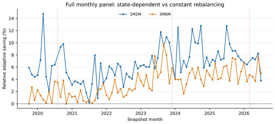
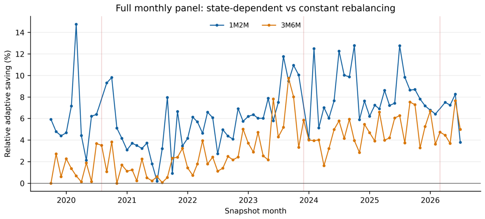
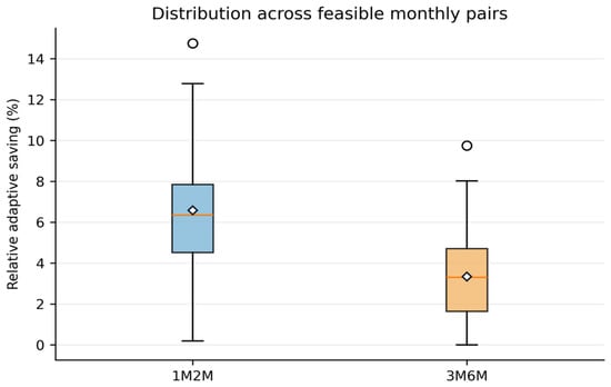
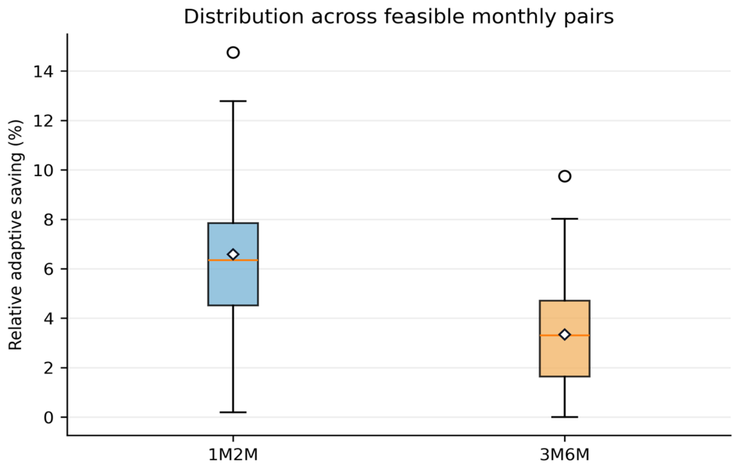
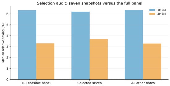
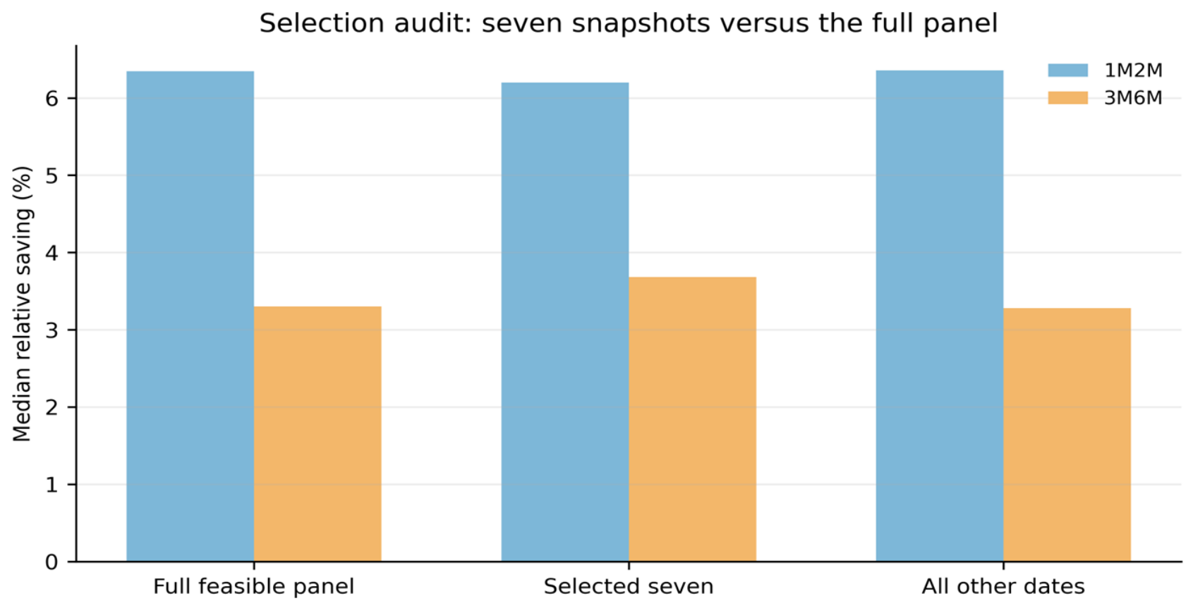
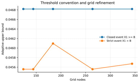
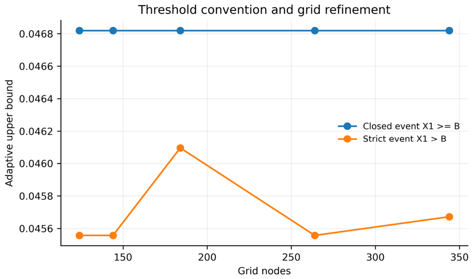
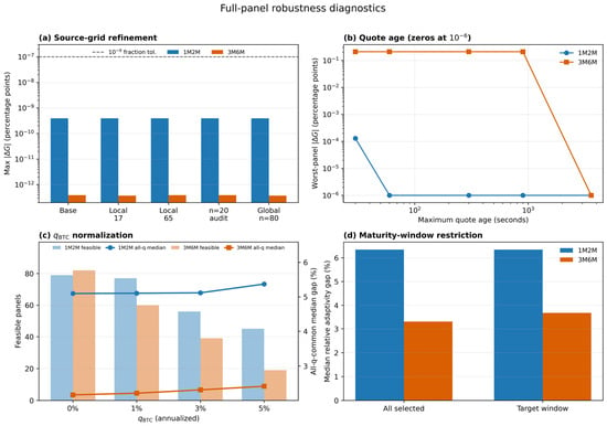
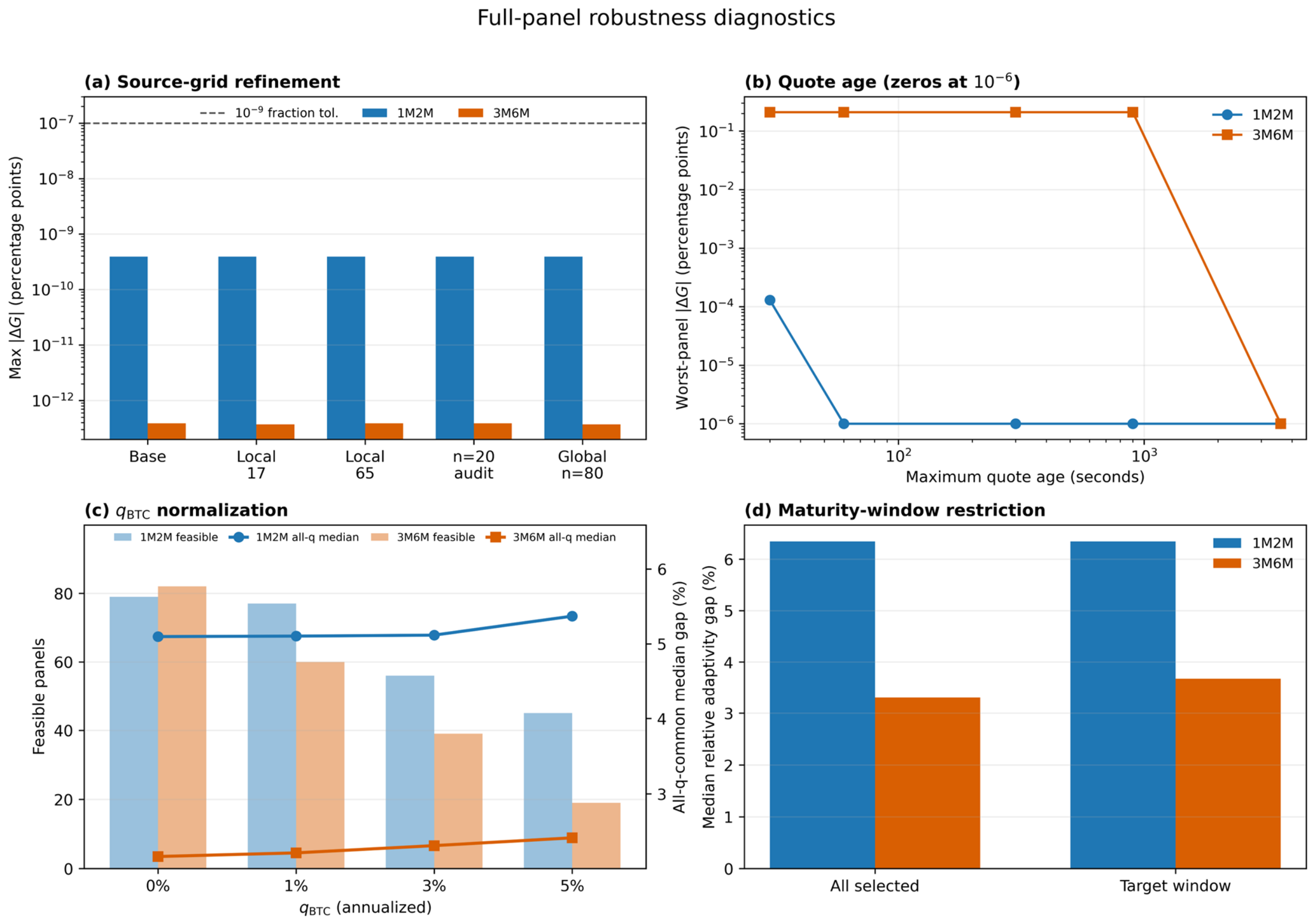
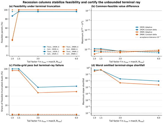
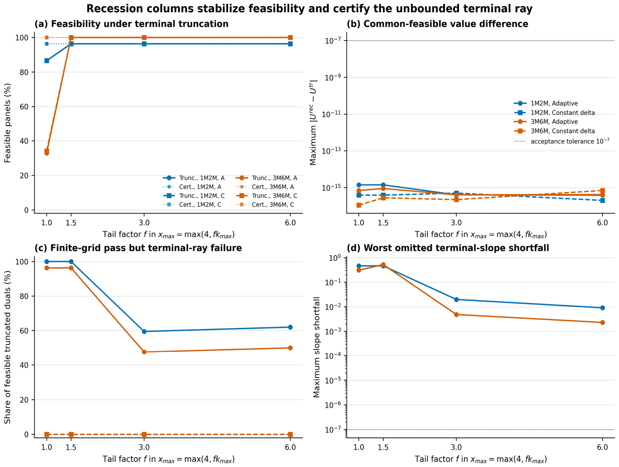
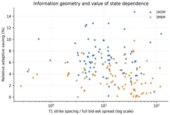
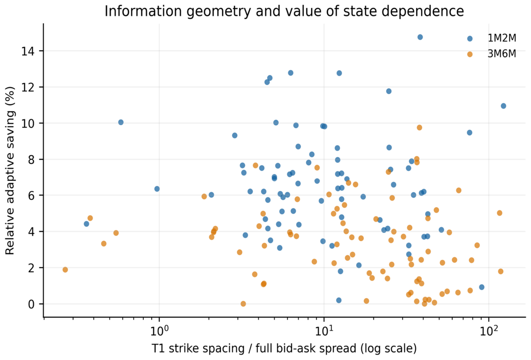
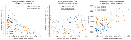
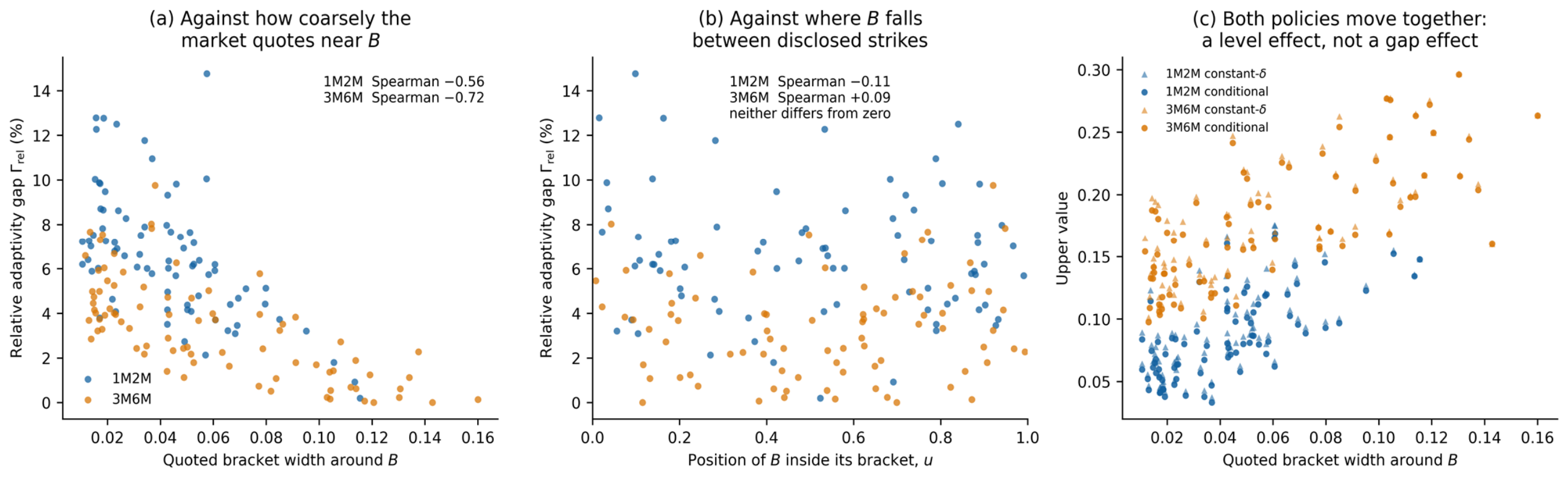
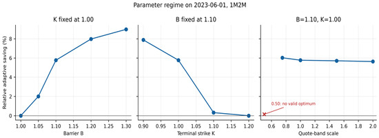
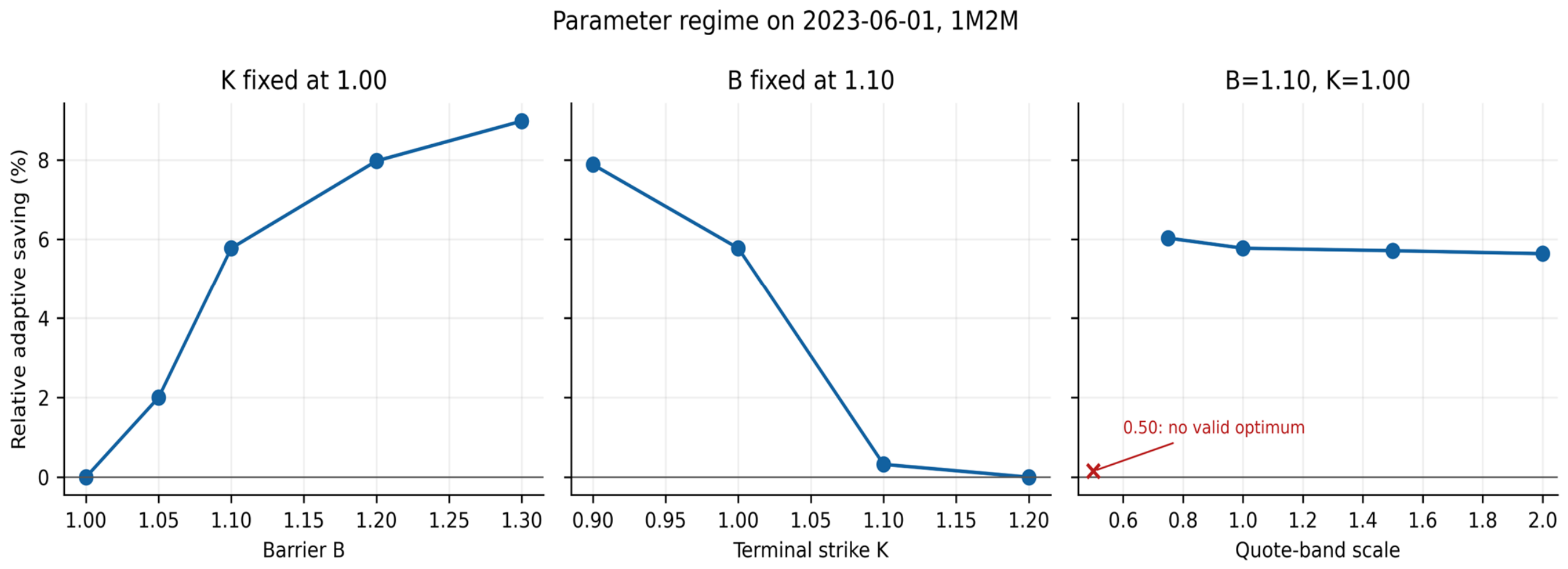
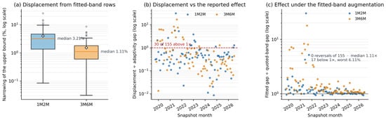
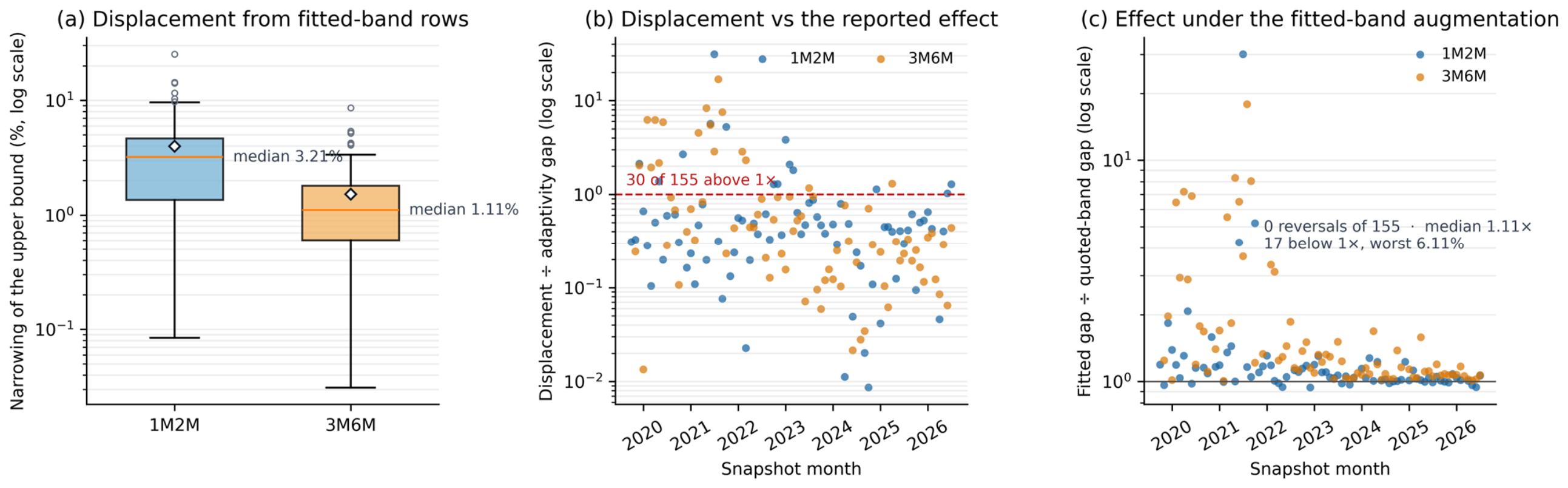
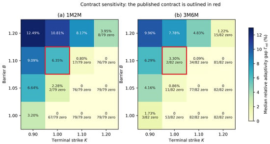
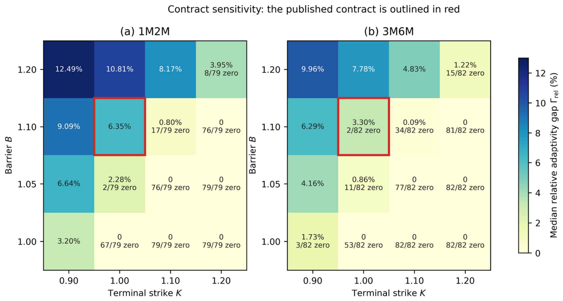

Disclaimer/Publisher’s Note: The statements, opinions and data contained in all publications are solely those of the individual author(s) and contributor(s) and not of MDPI and/or the editor(s). MDPI and/or the editor(s) disclaim responsibility for any injury to people or property resulting from any ideas, methods, instructions or products referred to in the content. |
© 2026 by the authors. Licensee MDPI, Basel, Switzerland. This article is an open access article distributed under the terms and conditions of the Creative Commons Attribution (CC BY) license.