On the Global Well-Posedness of a Non-Autonomous Reaction–Diffusion–Advection System Stemming from Alzheimer’s Modeling

Abstract

In this paper, we study the global well-posedness of a reaction–diffusion–advection system with time-dependent coefficients that models the interaction of ATM and ApoE proteins in cells under Alzheimer’s disease. We prove the existence and uniqueness of a non-negative global solution to this system considering in particular a non-autonomous advective term by demonstrating the existence of a local-in-time solution both with an autonomous and non-autonomous approach. The non-negativity of the solution is proven in the non-autonomous case and passed to the solution of the autonomous setting, and we compute energy estimates that show that this solution is in fact global.

1. Motivation and State of the Art

The study of global well-posedness for reaction–diffusion systems has been deeply investigated in recent years for autonomous problems and even for non-autonomous problems, but advection has often been neglected. In the case of autonomous reaction–diffusion systems, the global existence of a unique solution up to dimension 2 under quadratic growth in the reaction and satisfying non-negativity and entropy dissipation was proved in [1,2]. In [3,4,5], the authors independently established between 2017 and 2019 that a global solution exists for higher dimensions under entropy dissipation and mass control for autonomous reaction–diffusion systems, and, moreover, in [6] it was demonstrated that the solution is uniformly bounded instead of polynomially.

In the case of non-autonomous reaction–diffusion systems, there is a gap of 21 years between [7], where it was proven that a global classical solution for a non-autonomous system exists under strong constraints for the reaction, and 2021, where in [8], the authors showed that a unique global weak solution for the reaction–diffusion system exists for just measurable diffusion coefficients and a quadratic reaction, under mass control and intermediate sum conditions.

Later, the main result of [5] was extended in [9] into a particular non-autonomous system; in [10] it was shown that there exists a unique global classical solution in dimension 1 for a system with mass dissipation; and ref. [11] verifies the existence of a global weak solution for a non-autonomous reaction–diffusion system with fractional diffusion and mass control.

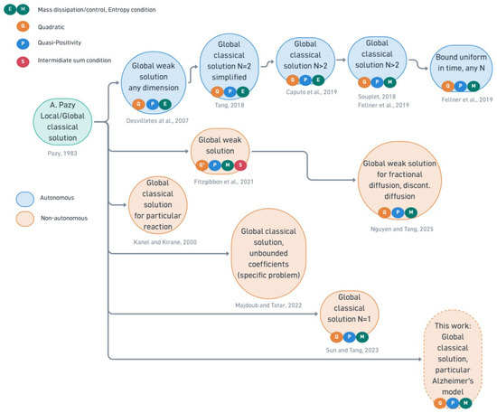
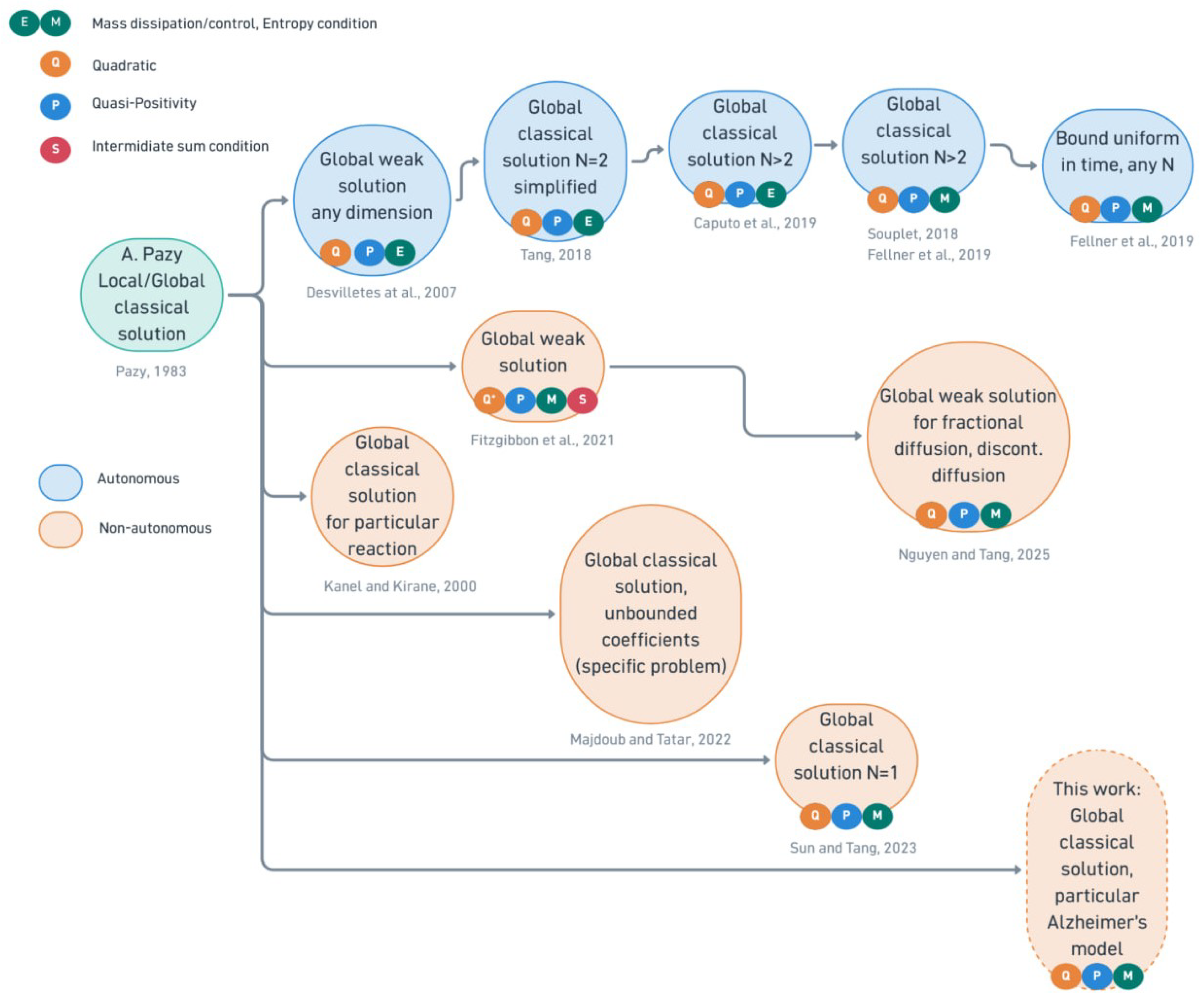
For systems including advection, ref. [8] shows that a unique global weak solution exists under quasi-positivity, mass control and an intermediate sum condition, meaning that the partial sum of the reactions in each equation is bounded by a polynomial of degree r, where $0\le r<1+{\displaystyle \frac{2}{n}}$, and n is the spatial dimension. This means that for $n\ge 2$, the quadratic terms need to “cancel out” and at least one of the equations need to be at most linear. Thus, for non-autonomous systems with advection, global well-posedness has so far been restricted to cases where a cancellation condition controls the quadratic terms or to one spatial dimension. In contrast, for the ATM–ApoE model we prove global existence and uniqueness up to dimension 4 without relying on any such cancellation. Figure 1 illustrates the developments in well-posedness results for reaction-diffusion systems.

Figure 1. State of the art on well-posedness of reaction–diffusion systems, building upon the foundational local/global classical solution results of Pazy [12]. For autonomous (blue) problems, the existence and uniqueness of a global solution have been proven in any dimension. For non-autonomous (orange) systems, the results have been proven for either specific problems, systems satisfying the intermediate sum condition, or problems without advection. The depicted works are, for autonomous problems: [1,2,3,4,5,6]; and for non-autonomous problems: [7,8,9,10,11].

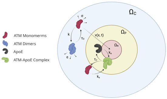
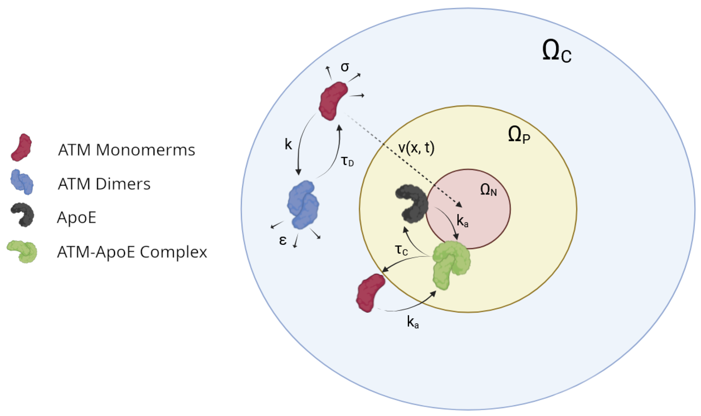
In this work, we show a proof for global existence and uniqueness of a non-negative solution up to dimension 4 by a semigroup and evolution systems argument. This works for our particular system with the quadratic polynomial reaction satisfying quasi-positivity, with time-dependent coefficients and for time-dependent advection coefficients, which is relevant in the context of ATM-ApoE interaction (Figure 2) and potential treatments controlling stress and the advection coefficient. The quasi-positivity is a natural property of the system, since the variables of the model represent protein concentrations. Even though we do not treat the long-term behavior of the solution in this work, it is worth mentioning that our well-posedness result provides the foundation for subsequent stability analyses, such as those for time-periodic traveling fronts [13], and for studies of asymptotic symmetry of solutions [14].

Figure 2. Diagram of spatial model interactions in a cell. Light blue shows the cytoplasm (${\Omega }_C$), yellow shows the area around the nucleus where the ApoE proteins are located (${\Omega }_P$), and pink shows the nucleus (${\Omega }_N$).

We prove the well-posedness of a system that models the interaction between proteins in cells affected by Alzheimer’s disease (AD). The importance of this model is that AD is the leading cause of dementia worldwide and it affects over 55 million people, with projections estimating a tripling of cases by 2050 [15]. Characterized by progressive neurodegeneration, memory loss, and cognitive decline, AD remains incurable despite decades of research. Current therapies focus on symptom management, since the cause of AD is unknown. AD is traditionally attributed to the accumulation of amyloid-$\beta$ ($A\beta$) plaques, tau protein neurofibrillary tangles, chronic neuroinflammation, and genetic factors such as the apolipoprotein E (ApoE) $\epsilon 4$ allele [16,17,18,19,20,21].

Recent radiobiological studies propose to focus on the Radiation-Induced ATM NucleoShuttling (RIANS) response [22]. This mechanism highlights the role of the Ataxia Telangiectasia Mutated (ATM) protein, a key mediator of DNA repair, and its interaction with ApoE (not necessarily $\epsilon 4$ allele). Under oxidative stress, ATM dimers dissociate into monomers that migrate to the nucleus to repair double-strand breaks (DSBs). However, in AD, overexpression of ApoE leads to the formation of ATM-ApoE complexes, which accumulate around the nucleus as a perinuclear crown (PC). This crown creates a barrier, impeding ATM’s nuclear entry and perpetuating unrepaired DNA damage, ultimately accelerating neuronal death [18].

2. Description of the Spatial Model

We study the well-posedness of a system that models the ATM-ApoE interaction. We propose a semilinear partial differential system of reaction–diffusion–advection equations that has four variables: M represents the concentration of ATM monomers while D denotes the concentration of ATM dimers, the variable A represents ApoE protein, and C the concentration of ATM-ApoE complexes. In this model, ATM monomers advect towards the nucleus of the cell to detect double-strand breaks (DSBs) in the DNA and repair them, due to an electrical signal sent by the nucleus. As mentioned before, DSBs may cause mutations or even cell death, so ATM is responsible for the repair of this DNA break. Oxidative stress monomerizes ATM dimers and ATM-ApoE complexes, allowing ATM to cross the nucleus membrane. ATM and ApoE tend to form dimers and complexes depending on different rates induced by oxidative stress, irradiation, and the intake of drugs. The complete interaction can be seen in Figure 2.

Consider $\Omega =B(0,1)\subseteq {\mathbb{R}}^n$ and an interval $[0,T],T>0$. Fix $\alpha \in (0,1)$.

$$\left\{\begin{array}{c}{\partial }_{t}M=\sigma \Delta M+div(v(t,x)M)-k{M}^2-dM\hfill \\ -k_{a}A·M+2{\tau }_D(t)D+{\tau }_C(t)C+\Lambda ,\hfill \\ {\partial }_{t}D=\epsilon \Delta D+0.5k{M}^2-{\tau }_D(t)D,\hfill \\ {\partial }_{t}A=\epsilon \Delta A-k_{a}A·M+{\tau }_C(t)C,\hfill \\ {\partial }_{t}C=\epsilon \Delta C+k_{a}A·M-{\tau }_C(t)C.\hfill \end{array}\right.$$

(1)

Here, the coefficients and parameters are:

• $\sigma ,\epsilon >0$: diffusion coefficients.
• $v(t,x)\in C^{\alpha }([0,T];C^{\infty }(\overline{\Omega }))$, zero at the boundary and divergence-free: transport of monomers towards the nucleus.
• $k>0$: rate of ATM dimer formation.
• $d>0$: rate of ATM monomer degradation.
• $k_a>0$: rate of ATM-ApoE complex formation.
• ${\tau }_D(t)\in C^{\alpha }([0,T])$ strictly positive and bounded: rate of monomerization of ATM due to oxidative stress.
• ${\tau }_C(t)\in C^{\alpha }([0,T])$ strictly positive and bounded: rate of monomerization of ATM-ApoE complex due to oxidative stress.
• $\Lambda >0$: rate of production of ATM monomers in the cell.

In order to simplify notation we write $v:=v(t,x),{\tau }_D:={\tau }_D(t),{\tau }_C:={\tau }_C(t)$. We consider the following non-autonomous system of reaction–diffusion–advection equations for $(M,D,A,C)$:

$$\left\{\begin{array}{c}{\partial }_{t}M=\sigma \Delta M+div(vM)-k{M}^2-dM-k_{a}A·M+2{\tau }_{D}D+{\tau }_{C}C+\Lambda ,\hfill \\ {\partial }_{t}D=\epsilon \Delta D+0.5k{M}^2-{\tau }_{D}D,\hfill \\ {\partial }_{t}A=\epsilon \Delta A-k_{a}A·M+{\tau }_{C}C,\hfill \\ {\partial }_{t}C=\epsilon \Delta C+k_{a}A·M-{\tau }_{C}C,\hfill \end{array}\right.$$

(2)

with boundary and initial conditions

$$\left\{\begin{array}{c}\nabla M·n=0,\partial \Omega \times [0,T],\hfill \\ \nabla D·n=0,\partial \Omega \times [0,T],\hfill \\ \nabla A·n=0,\partial \Omega \times [0,T],\hfill \\ \nabla C·n=0,\partial \Omega \times [0,T],\hfill \\ (M,D,A,C)(0,·)=(M_0,D_0,A_0,C_0)=:u_0,\Omega \times \left\{0\right\}.\hfill \end{array}\right.$$

The choice of boundary conditions are due to the fact that none of these proteins exit the cell’s membrane; therefore, we consider homogeneous Neumann boundary conditions. When convenient, we write the system in the general form:

$${\partial }_{t}u=D\Delta u+V(t,x)·\nabla u+F(t,u),$$

(3)

with boundary and initial conditions

$$\left\{\begin{array}{c}\nabla u·n=0,\partial \Omega \times [0,T],\hfill \\ u(0,·)=u_0,\Omega \times \left\{0\right\},\hfill \end{array}\right.$$

where D is a diagonal matrix, $V(t,x):={(v(t,x),0,0,0)}^T\in C^{\alpha }([0,T];C^{\infty }{(\overline{\Omega })}^4)$ is the advection coefficient and $F(t,u):{\mathbb{R}}^{+}\times {\left[H^1\right]}^4\to {\left[L^2\right]}^4$ is the reaction term.

3. Main Result

First, let us define what a solution is; we provide a definition of a global classical solution for system (2, 3):

Definition 1 (Solution).

Let $X:=L^2(\Omega )$ be a Banach space and let $A_N$ be the realization of $-\Delta$ in $L^2(\Omega )$ with homogeneous Neumann boundary conditions. Let $X^{{\displaystyle \frac{1}{2}}}:=D(A_N^{{\displaystyle \frac{1}{2}}})=H^1(\Omega )$ Banach with the graph norm ${\parallel x\parallel }_{{\displaystyle \frac{1}{2}}}:=\parallel A_I^{{\displaystyle \frac{1}{2}}}x\parallel$, where $A_I:=A_N+bI$ with b chosen such that Re $\sigma (A_I)>0$ (the choice of b produces equivalent norms). We say that a continuous function $u:[0,T)\to X$ is a solution of system (3) in $[0,T)$ if for $F(t,u)+V(t,x)·\nabla u:=\tilde{F}(t,u):U\to X$, $U\subseteq \mathbb{R}\times X^{{\displaystyle \frac{1}{2}}}$, u satisfies the equation pointwise in $(0,T)$, u is continuously differentiable on $(0,T)$, $(t,u(t))\in U$ and $u(t)\in D{A}_N$ for every $t\in (0,T)$ with $u(t)\to u_0$ as $t\to 0^{+}$.

Remark 1.

We say that the solution is global if there is a solution in $[0,T_{\mathit{max}})$, where $T_{\mathit{max}}$ is maximal and $T_{\mathit{max}}=+\infty$.

The goal of this work is to prove the following well-posedness theorem:

Theorem 1.

If $u_0\in C^1(\overline{\Omega })$ is non-negative, then there exists a unique global classical non-negative solution of system (2).

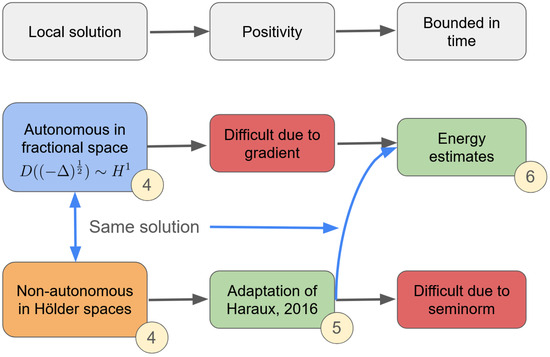
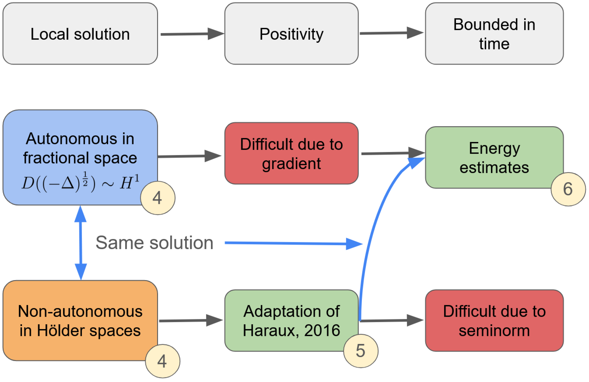
In the following sections we prove the non-negativity and the existence of a unique global classical solution to problems (2, 3). The proof for existence/uniqueness of a local-in-time solution is addressed in Section 4, the proof of non-negativity in Section 5 follows from [23] for a non-autonomous system and then passed to the solution of the autonomous problem, and in Section 6 we give a bound for the solution which gains regularity by a bootstrap argument, ensuring the solution is in fact global in time. The scheme of the proof is represented in Figure 3.

Figure 3. Scheme of the proof numbered by section. We prove the existence of the local solution in both settings (Section 4) and prove the positivity in the non-autonomous case by the argument in [23] (Section 5). We pass this property to the solution of the autonomous setting and prove estimates (Section 6) that show that the solution is global.

4. Local in Time Solution

We consider the general form of the system, i.e.,

$${\partial }_{t}u=D\Delta u+V(t,x)·\nabla u+F(t,u),$$

with boundary and initial conditions

$$\left\{\begin{array}{c}\nabla u·n=0,\partial \Omega \times [0,T],\hfill \\ u(0,·)=u_0,\Omega \times \left\{0\right\}.\hfill \end{array}\right.$$

Since the advection coefficient depends on time, we consider it as part of the reaction term to apply the semigroup theory for autonomous problems. The domain of the operator needs to take into account that $\nabla u$ must be well defined, so we define the problem over $D(A_N^{{\displaystyle \frac{1}{2}}})\sim H^1$. To apply the existence result from [24] (p. 54, Theorem 3.3.3), we need the reaction to be locally Lipschitz on u. We check that

$$\tilde{F}(t,u)=F(t,u)+V(t,x)·\nabla u,$$

defined from ${\mathbb{R}}^{+}\times {\mathit{H}}^{\mathbf{1}}\to {\mathit{L}}^{\mathbf{2}}$ is locally Lipschitz in u, where ${\mathit{H}}^{\mathbf{1}}:={\left[H^1\right]}^4$ and ${\mathit{L}}^{\mathbf{2}}:={\left[L^2\right]}^4$. Since F is quadratic in u, let us consider only the term $u^2$,

$${\parallel F(t,u)-F(t,v)\parallel }_{{\mathit{L}}^{\mathbf{2}}}\le {\parallel u+v\parallel }_{{\mathit{L}}^{\mathbf{4}}}{\parallel u-v\parallel }_{{\mathit{L}}^{\mathbf{4}}},$$

since $H^1$ is embedded in $L^4$ for dimension $d\le 4$ [Gagliardo–Nirenberg], then

$${\parallel F(t,u)-F(t,v)\parallel }_{{\mathit{L}}^{\mathbf{2}}}\le {C(\parallel u\parallel }_{{\mathit{H}}^{\mathbf{1}}}+{\parallel v\parallel }_{{\mathit{H}}^{\mathbf{1}}}{)\parallel u-v\parallel }_{{\mathit{H}}^{\mathbf{1}}}.$$

For the advection term, since we assume $v\in C^{\alpha }([0,T];C^{\infty }(\overline{\Omega }))$,

$${\parallel V·\nabla u\parallel }_{{\mathit{L}}^{\mathbf{2}}}\le {\parallel V\parallel }_{{\mathit{L}}^{\infty }}{\parallel u\parallel }_{{\mathit{H}}^{\mathbf{1}}}.$$

So $\tilde{F}$ is locally Lipschitz from ${\mathit{H}}^{\mathbf{1}}$ to ${\mathit{L}}^{\mathbf{2}}$. Since all the coefficients are locally Hölder continuous in t, existence and uniqueness follow from [24] (p. 54, Theorem 3.3.3).

Local Solution in Non-Autonomous Setting

It is useful in the next section to consider the local solution in the context of a non-autonomous problem defined in Hölder spaces, i.e., the time-dependent advection coefficient is considered as part of the operator instead of as part of the reaction term, so in this section we consider $X=C^{\alpha }(\overline{\Omega })$. We provide the necessary conditions to have such a solution.

Proposition 1.

Consider the system:

$${\partial }_{t}u+A(t)u=f(t,u),u(s)=u_0,\nabla u·n=0.$$

Let $f:[s,T]\times X\to X$ be Hölder continuous in t on $[s,T]$ and uniformly Lipschitz continuous (with constant L) on X. Let $A(t)$ satisfy the following assumptions:

(P₁) 

The domain $D(A(t))=D$ of $A(t)$, $0\le t\le T$ is dense in X and independent of t;

(P₂) 

For $t\in [0,T]$, the resolvent $R(\lambda :A(t))$ of $A(t)$ exists for all λ with Re $\lambda \le 0$ and there is a constant M such that

$$\parallel R(\lambda :A(t))\parallel \le {\displaystyle \frac{M}{|\lambda |+1}},\mathit{for}\mathit{Re}\lambda \le 0,t\in [0,T],$$

(P₃) 

There exist constants L and $0<\alpha \le 1$ such that

$${\parallel (A(t)-A(s))A(\tau )}^{-1}{\parallel \le L|t-s|}^{\alpha },\mathit{for}s,t,\tau \in [0,T],$$

And let $U(t,s)$ be the associated evolution system [12] (p. 168, Theorem 7.1, Chapter 5). Then, the initial value problem has a unique mild solution $u\in C([s,T];X)$. Moreover, the mapping $u_0\to u$ is Lipschitz continuous from X into $C([s,T];X)$.

Remark 2.

These are two classical results from [12] presented as one for simplicity.

Proof. 

For a given $u_0\in X$ we define a mapping

$$F:C([s,T];X)\to C([s,T];X),$$

by

$${\displaystyle (Fu)(t)=U(t,s)u_0+{\int }_s^{t}U(t,r)f(r,u(r))dr,s\le t\le T.}$$

Denoting by ${\parallel u\parallel }_{\infty }$ the norm of u as an element of $C([s,T];X)$, it follows readily from the definition of F that

$$\parallel (Fu)(t)-(Fv)(t)\parallel \le {CL(t-s)\parallel u-v\parallel }_{\infty },$$

where C is a bound of $\parallel U(t,s)\parallel$ on $[s,T]$ by [12] (Chapter 5). By induction on k it follows that

$$\parallel (F^{k}u)(t)-(F^{k}v)(t)\parallel \le {\displaystyle \frac{{(CL(t-s))}^k}{k!}}{\parallel u-v\parallel }_{\infty },$$

and so

$$\parallel F^{k}u-F^{k}v\parallel \le {\displaystyle \frac{{(CLT)}^k}{k!}}{\parallel u-v\parallel }_{\infty }.$$

For k large enough ${\displaystyle \frac{{(CLT)}^k}{k!}}<1$, F has a unique fixed point u in $C([s,T];X)$. This fixed point is the desired solution of the system. The uniqueness of u and the Lipschitz continuity of the map $u_0\to u$ are consequences of the following argument. Let v be a mild solution on $[s,T]$ with the initial value $v_0$. Then,

$$\begin{array}{cc}\hfill \parallel u(t)-v(t)\parallel & {\displaystyle \le \parallel U(t,s)u_0-U(t,s)v_0\parallel +{\int }_s^t\parallel U(t,r)(f(r,u(r))-f(r,v(r)))dr}\hfill \\ \hfill & {\displaystyle \le C\parallel u_0-v_0\parallel +CL{\int }_s^t\parallel u(r)-v(r)\parallel dr,}\hfill \end{array}$$

which implies by Gronwall’s inequality that

$$\parallel u(t)-v(t)\parallel \le C{e}^{CL(T-s)}\parallel u_0-v_0\parallel ,$$

and therefore

$${\parallel u-v\parallel }_{\infty }\le C{e}^{CL(T-s)}\parallel u_0-v_0\parallel ,$$

which yields both the uniqueness of u and the Lipschitz continuity of the map $u_0\to u$.  □

In the previous proposition, the uniform Lipschitz condition on f assures the existence of a global mild solution. If f is assumed to be locally Lipschitz continuous in its second variable, then we have existence of a local mild solution. This proof is a classical result from [12], where we have made explicit, for the convenience of the reader, the changes made for evolution systems.

Corollary 1.

Let $f:[0,+\infty )\times X\to X$ be continuous in t for $t\ge 0$ and locally Lipschitz continuous in u, uniformly in t on bounded intervals. Consider the system and assumptions in Proposition 1. Then, for every $u_0\in X$ there is a $t_{max}\le +\infty$ such that the initial value problem has a unique mild solution u on $[0,t_{max})$. Moreover, if $t_{max}<+\infty$, then

$$\underset{t\uparrow t_{max}}{lim}\parallel u(t)\parallel =\infty .$$

Proof. 

Let $L(c,t^{\prime })$ be the Lipschitz constant of f in the ball of radius c with $t\in [0,t^{\prime }]$, i.e.,

$$\parallel f(t,u)-f(t,v)\parallel \le L(c,t^{\prime })\parallel u-v\parallel ,$$

for all $u,v\in X$ such that $\parallel u\parallel \le c,\parallel v\parallel \le c$. For every $s\ge 0$, $u_0\in X$, the initial value problem has a unique mild solution u on an interval $[s,t_1]$, whose length is bounded below by

$$\delta (s,\parallel u_0\parallel )=min\left\{1,{\displaystyle \frac{\parallel u_0\parallel }{K(s)L(K(s),s+1)+N(s)}}\right\},$$

where $M(s)=sup\{\parallel U(t,s)\parallel :0\le t\le s+1\}$, $K(s)=2\parallel u_0\parallel M(s)$ and $N(s)=sup\{\parallel f(t,0)\parallel :0\le t\le s+1\}$. Indeed, let $t_1=s+\delta (s,\parallel u_0\parallel )$. The mapping F defined in Proposition 1 maps the ball of radius $K(s)$ centered at 0 of $C([s,t_1];X)$ into itself. This follows from the estimate

$$\begin{array}{cc}\hfill \parallel (Fu)(t)\parallel & {\displaystyle \le M(s)\parallel u_0\parallel +{\int }_s^t\parallel U(t,r)\parallel (\parallel f(r,u(r))-f(r,0)\parallel +\parallel f(r,0)\parallel )dr}\hfill \\ \hfill & \le M(s)\parallel u_0\parallel +M(s)K(s)L(K(s),s+1)(t-s)+M(s)N(s)(t-s)\hfill \\ \hfill & \le M(s)\left[\parallel u_0\parallel +K(s)L(K(s),s+1)(t-s)+N(s)(t-s)\right]\hfill \\ \hfill & \le 2M(s)\parallel u_0\parallel \hfill \\ \hfill & =K(s),\hfill \end{array}$$

where the last inequality follows from the definition of $t_1$. In this ball, F satisfies a uniform Lipschitz condition with constant $L=L(K(s),s+1)$ and thus it possesses a unique fixed point u in the ball. This fixed point is the mild solution of the initial value problem in the interval $[s,t_1]$. If u is a mild solution on the interval $[0,\tau ]$, it can be extended to the interval $[0,\tau +\delta ]$ with $\delta >0$ by defining on $[\tau ,\tau +\delta ]$, $u(t)=w(t)$, where $w(t)$ is the solution of the integral equation

$${\displaystyle w(t)=U(t,\tau )u(\tau )+{\int }_{\tau }^{t}U(t,r)f(r,w(r))dr,\tau \le t\le \tau +\delta .}$$

Moreover, $\delta$ depends only on $\parallel u(\tau )\parallel ,K(\tau )$ and $N(\tau )$.

Let $[0,t_{max})$ be the maximal interval of existence of the mild solution u. If $t_{max}<+\infty$ then ${lim}_{t\uparrow t_{max}}\parallel u(t)\parallel =\infty$ since otherwise there is a sequence $t_n\uparrow t_{max}$ such that $\parallel u(t_n)\parallel \le C$ for all n. This would imply by what we have just proved that for each $t_n$, near enough to $t_{max}$, u defined on $[0,t_n]$ can be extended to $[0,t_n+\delta ]$, where $\delta$ is independent of $t_n$ and hence u can be extended beyond $t_{max}$, contradicting the definition of $t_{max}$. To prove the uniqueness of the local mild solution u of the initial value problem, we note that if v is another mild solution, then on every closed interval $[0,s]$ on which both u and v exist, they coincide by the uniqueness argument given at the end of Proposition 1. Therefore, both u and v have the same $t_{max}$ and on $[0,t_{max})$, $u\equiv v$.  □

In [12] (p. 227, Lemma 6.1, Chapter 7) and [12] (p. 228, Theorem 6.2, Chapter 7), the author proves the existence of a solution in $L^p$ for a family of operators satisfying two conditions that are easier to verify than (P1), (P2), and (P3). The following proposition gathers both results adapted to $C^{\alpha }$. For completeness, we prove it in the case of $C^{\alpha }$ following exactly the steps in [12] with the exception of one inequality which is proved in Lemma 1.

Proposition 2 (Alternative conditions).

For $X=C^{\alpha }$, let the family of operators $A(t),t\in [0,T]$ in $C^{\alpha }$ be defined as the realization of

$${\displaystyle A(t,x)=\sum _{|\beta |=2m}{a}_{\beta }(x)D^{\beta }+\sum _{|\beta |<2m}{a}_{\beta }(t,x)D^{\beta },}$$

in $C^{\alpha }$, i.e.,

$$D(A(t))=D(A)=\left\{u\in C^{2m,\alpha }(\overline{\Omega }):B_j(x)u=0\mathit{on}\partial \Omega ,j=0,\dots ,m-1\right\},$$

with $B_j(x)$ boundary differential operators derived from $a_{\beta }(t,x)$ and

$$A(t)u=A(t,x)u,\mathit{for}u\in D(A).$$

If this family satisfies the following conditions:

(H₁) 

The operators $A(t,x),t\ge 0$ are uniformly elliptic in Ω, i.e., there is a constant $c>0$ such that

$${\displaystyle {(-1)}^m\mathit{Re}\sum _{|\beta |=2m}{a}_{\beta }(t,x){\xi }^{\beta }\ge c{|\xi |}^{2m},}$$

for every $x\in \overline{\Omega },0\le t\le T$ and $\xi \in {\mathbb{R}}^d$,

(H₂) 

The coefficients $a_{\beta }(t,x)$ are smooth functions of the variables x in $\overline{\Omega }$ for every $0\le t\le T$ and satisfy, for some constants $C_1>0$ and $0<\delta \le 1$,

$$|a_{\beta }(t,x)-a_{\beta }(s,x)|\le C_1{|t-s|}^{\delta },$$

for $x\in \overline{\Omega },0\le s\le t\le T$ and $|\beta |\le 2m$,

then the family $\{A_p(t)+kI\}$ satisfies (P1)–(P3). And if $A(t,x)$ satisfies (H1), (H2) and $f\in C^{\alpha }(\overline{\Omega })$ satisfies

$${\parallel f(t,x)-f(s,x)\parallel }_{C^{\alpha }}\le C{|t-s|}^{\gamma },$$

for some constants $C>0$ and $0\le \gamma <1$, then for every $u_0(x)\in C^{\alpha }$ the linear problem

$$\left\{\begin{array}{c}{\displaystyle \frac{du}{dt}}+A(t)u=f,\hfill \\ u(0)=u_0,\hfill \end{array}\right.$$

has a unique solution. Moreover, if $f:[t_0,T]\times C^{\alpha }\to C^{\alpha }$ is Hölder continuous in t on $[0,T]$ and locally Lipschitz continuous on $C^{\alpha }$, uniformly in t on bounded intervals, then for every $u_0\in C^{\alpha }$ the nonlinear problem

$$\left\{\begin{array}{c}{\displaystyle \frac{du}{dt}}+A(t)u=f(t,u),\hfill \\ u(0)=u_0,\hfill \end{array}\right.$$

has a unique solution.

Proof. 

From the definition of the operators $A(t)$, and since we assume $a_{\beta }(t,x)=a_{\beta }(x)$ for $|\beta |=2m$, the boundary operators $B_j$ are independent of t. It follows that for every real k, the domain of $D(A(t)+kI)=D(A(t))=D$ independent of t and therefore, for any choice of $k\ge 0$, the family ${\{A_p(t)+kI\}}_{t\in [0,T]}$ satisfies the condition (P1). By Lemma 1 proven below, we have

$${\parallel u\parallel }_{C^{\alpha }}\le {\displaystyle \frac{M}{|\lambda |}}{\parallel (\lambda I+A(t))u\parallel }_{C^{\alpha }},$$

(4)

for $u\in D$ and $\lambda$ satisfying Re $\lambda \ge 0$ and $|\lambda |\ge R$ for some constant $R\ge 0$. Choosing $k>R$, (4) implies that

$$\begin{array}{cc}\hfill {\parallel u\parallel }_{C^{\alpha }}& \le {\displaystyle \frac{M_1}{|\lambda +k|}}{\parallel (\lambda I+(A(t)+kI))u\parallel }_{C^{\alpha }}\hfill \\ \hfill & \le {\displaystyle \frac{M}{|\lambda |+1}}{\parallel (\lambda I+A(t)+kI)u\parallel }_{C^{\alpha }},\hfill \end{array}$$

holds for $u\in D$ and $\lambda$ satisfying Re $\lambda \ge 0$. Using [25] (Theorem 3.1.32), $A(t)+kI$ is sectorial and therefore

$${\parallel R(\lambda :A(t)+kI)u\parallel }_{C^{\alpha }}\le {\displaystyle \frac{M}{1+|\lambda |}}{\parallel u\parallel }_{C^{\alpha }},$$

for $u\in C^{\alpha }$. Therefore, fixing $k>R$ implies that the family ${\{A_p(t)+kI\}}_{t\in [0,T]}$ satisfies (P2). For $u\in C^{\alpha }$ and $w={(A(\tau )+kI)}^{-1}u$ we have $w\in D$ and

$$\begin{array}{cc}\hfill {∥(A(t)+kI)w-(A(s)+kI)w∥}_{C^{\alpha }}& {\displaystyle =\parallel \sum _{|\beta |\le 2m}(a_{\beta }(t,x)-a_{\beta }(s,x))D^{\beta }{w\parallel }_{C^{\alpha }}}\hfill \\ \hfill & {\displaystyle \le C_1{|t-s|}^{\delta }\sum _{|\beta |\le 2m}{\parallel D^{\beta }w\parallel }_{C^{\alpha }}}\hfill \\ \hfill & \le C_2{|t-s|}^{\delta }{\parallel w\parallel }_{C^{2,\alpha }}.\hfill \end{array}$$

Then, from estimates (4) and (6),

$$\begin{array}{cc}\hfill {\parallel w\parallel }_{C^{2,\alpha }}& \le C(\parallel A(\tau ){(A(\tau )+kI)}^{-1}u{\parallel }_{C^{\alpha }}+\parallel {(A(\tau )+kI)}^{-1}u{\parallel }_{C^{\alpha }})\hfill \\ \hfill & \le {C(1+kM+M)\parallel u\parallel }_{C^{\alpha }}.\hfill \end{array}$$

Combining these inequalities yields

$${\parallel ((A(t)+kI)-(A(s)+kI))(A(\tau )+kI)}^{-1}{u\parallel }_{C^{\alpha }}\le C_3{|t-s|}^{\delta }{\parallel u\parallel }_{C^{\alpha }},$$

for every $u\in C^{\alpha }$, so the family ${\{A_p(t)+kI\}}_{t\in [0,T]}$ also satisfies the condition (P3). Finally, if $f\in C^{\alpha }(\overline{\Omega })$ satisfies

$${\parallel f(t,x)-f(s,x)\parallel }_{C^{\alpha }}\le C{|t-s|}^{\gamma },$$

for some constants $C>0$ and $0\le \gamma <1$, then there exists $C^{\prime }>0$ such that

$$\parallel e^{-kt}f(t,x)-e^{-ks}{f(s,x)\parallel }_{C^{\alpha }}\le C^{\prime }{|t-s|}^{\gamma },$$

(5)

for any real k. That being said, since we chose $k>R\ge 0$, we take advantage of this to simplify the computations. Indeed,

$$e^{-kt}f(t,x)-e^{-ks}f(s,x)=e^{-kt}f(t,x)-e^{-kt}f(s,x)+e^{-kt}f(s,x)-e^{-ks}f(s,x),$$

so

$$\parallel e^{-kt}f(t,x)-e^{-ks}{f(s,x)\parallel }_{C^{\alpha }}\le \parallel e^{-kt}f(t,x)-e^{-kt}{f(s,x)\parallel }_{C^{\alpha }}+{\parallel e^{-kt}f(s,x)-e^{-ks}f(s,x)\parallel }_{C^{\alpha }}.$$

The first term is bounded by

$$\begin{array}{cc}\hfill \parallel e^{-kt}f(t,x)-e^{-kt}{f(s,x)\parallel }_{C^{\alpha }}& \le e^{-kt}{\parallel f(t,x)-f(s,x)\parallel }_{C^{\alpha }}\hfill \\ \hfill & \le {\parallel f(t,x)-f(s,x)\parallel }_{C^{\alpha }}\hfill \\ \hfill & \le {C|t-s|}^{\gamma }.\hfill \end{array}$$

The second term is bounded by

$$\begin{array}{cc}\hfill \parallel e^{-kt}f(s,x)-e^{-ks}{f(s,x)\parallel }_{C^{\alpha }}& \le |e^{-kt}-e^{-ks}{|\parallel f(s,x)\parallel }_{C^{\alpha }}.\hfill \end{array}$$

The norm ${\parallel f(s,x)\parallel }_{C^{\alpha }}$ can be bounded independently of s. Indeed,

$${\parallel f(s,x)-f(0,x)\parallel }_{C^{\alpha }}\le C{|s|}^{\gamma }\le C{T}^{\gamma }.$$

Thus, for every $s\in [0,T]$,

$$\begin{array}{cc}\hfill {\parallel f(s,x)\parallel }_{C^{\alpha }}& \le {\parallel f(s,x)-f(0,x)\parallel }_{C^{\alpha }}+{\parallel f(0,x)\parallel }_{C^{\alpha }}\hfill \\ \hfill & \le C{T}^{\gamma }+{\parallel f(0,x)\parallel }_{C^{\alpha }}\hfill \\ \hfill & :=M.\hfill \end{array}$$

Since $h(\tau )=e^{-k\tau }$ is Lipschitz continuous with constant $L_k:=k$, then

$$\begin{array}{cc}\hfill \parallel e^{-kt}f(s,x)-e^{-ks}{f(s,x)\parallel }_{C^{\alpha }}& \le kM|t-s|\hfill \\ \hfill & \le kM{T}^{1-\gamma }{|t-s|}^{\gamma },\hfill \end{array}$$

where the last inequality comes from the fact that

$$|t-s|={|t-s|}^{1-\gamma }{|t-s|}^{\gamma }\le T^{1-\gamma }{|t-s|}^{\gamma }.$$

Taking $C^{\prime }:=C+kM{T}^{1-\gamma }$ yields inequality (5). Given $u_0\in C^{\alpha }$, the initial value problem

$$\left\{\begin{array}{c}{\displaystyle \frac{dv}{dt}}+(A(t)+kI)u=e^{-kt}f,\hfill \\ v(0)=u_0,\hfill \end{array}\right.$$

has a unique classical solution v by Proposition 1. Then, $u:=e^{kt}v$ is the unique solution of the initial value problem

$$\left\{\begin{array}{c}{\displaystyle \frac{dv}{dt}}+A(t)u=f,\hfill \\ u(0)=u_0.\hfill \end{array}\right.$$

The same argument is used for the nonlinear initial value problem.  □

Lemma 1.

Let $A(t)$ be the realization of ${\displaystyle A(t,x):=\sum _{|\beta |=2m}{a}_{\beta }(x)D^{\beta }+\sum _{|\beta |<2m}{a}_{\beta }(t,x)D^{\beta }}$ in $X:=C^{\alpha }$ with Neumann boundary conditions, i.e.,

$$D(A(t)):=\left\{u\in C^{2m,\alpha }(\overline{\Omega }):B_j(x)u=0\mathit{on}\partial \Omega ,j=0,\dots ,m-1\right\},$$

with $B_j$ boundary differential operators derived from $a_{\beta }(t)$. For λ sufficiently large in the ray arg $\lambda =\theta$ and $u\in D(A(t))$,

$${\parallel u\parallel }_{C^{\alpha }}\le {\displaystyle \frac{M}{|\lambda |}}{\parallel (\lambda I+A(t))u\parallel }_{C^{\alpha }}.$$

Proof. 

By [26] (Theorem 5), we have the estimate

$${\parallel u\parallel }_{C^{2,\alpha }}\le {C(\parallel A(t)u\parallel }_{C^{\alpha }}+{\parallel u\parallel }_{C^{\alpha }}).$$

(6)

Let $L:=A(t)+e^{i\theta }{\partial }_t^2$, $\Gamma :=\{(x,t):x\in \Omega ,t\in \mathbb{R}\}$ and ${\Gamma }_r$ be the restriction of $\Gamma$ to $|t|\le r$. By changing the norm of the estimate, we do not change the notion of ellipticity given in [27], and since the operator L is the same as in [12] (Chapter 7.3), it is elliptic and satisfies, like $A(t)$, the same estimate (6). Let $v_{\mu }:=\eta (t)e^{i\mu t}u(x)$, where $\eta (t)$ is a $C^{\infty }$ cutoff function such that $\eta (t)\equiv 0$ for $|t|\ge 1$ and $\eta (t)\equiv 1$ for $|t|\le {\displaystyle \frac{1}{2}}$, and $\mu$ is to be chosen later. Then, by applying L we obtain

$$L{v}_{\mu }=\eta (t)e^{i\mu t}(A-{\mu }^2{e}^{i\theta })u(x)+e^{i\theta }[{\eta }^{\prime \prime }(t)+2i{\eta }^{\prime }(t)]e^{i\mu t}u(x).$$

By definition of $v_{\mu }$ and by using estimate (6) on L,

$$\begin{array}{cc}\hfill \parallel u(x)e^{i\mu t}{\parallel }_{C^{2,\alpha }({\Gamma }_{1/2})}& \le \parallel v_{\mu }{\parallel }_{C^{2,\alpha }({\Gamma }_1)},\hfill \\ \hfill & \le C_1{[\parallel (A-\lambda I)u\parallel }_{C^{\alpha }}+{|\mu |\parallel u\parallel }_{C^{\alpha }}],\hfill \end{array}$$

where $\lambda :={|\mu |}^2{e}^{i\theta }$. Now, we check that $\parallel u(x)e^{i\mu t}{\parallel }_{C^{2,\alpha }({\Gamma }_{1/2})}\ge {|\mu |}^2{\parallel u\parallel }_{C^{\alpha }(\overline{\Omega })}$,

$$\begin{array}{cc}\hfill \parallel u(x)e^{i\mu t}{\parallel }_{C^{2,\alpha }({\Gamma }_{1/2})}& {\displaystyle =\sum _{|\gamma |\le 2}{\parallel D^{\gamma }(u{e}^{i\mu t})\parallel }_{C^2({\Gamma }_{1/2})}+\underset{|\beta |=2}{max}{\left[D^{\beta }(u{e}^{i\mu t})\right]}_{C^{0,\alpha }({\Gamma }_{1/2})},}\hfill \\ \hfill & \ge {|\mu |}^2{\parallel u\parallel }_{\infty }+{|\mu |}^2{\left[u{e}^{i\mu t}\right]}_{C^{0,\alpha }(\overline{\Omega })},\hfill \\ \hfill & ={|\mu |}^2{\parallel u\parallel }_{\infty }+{|\mu |}^2{\left[u\right]}_{C^{0,\alpha }(\overline{\Omega })},\hfill \\ \hfill & ={|\mu |}^2{\parallel u\parallel }_{C^{0,\alpha }(\overline{\Omega })},\hfill \\ \hfill & ={|\mu |}^2{\parallel u\parallel }_{C^{\alpha }(\overline{\Omega })}.\hfill \end{array}$$

Then, by combining the two inequalities,

$${|\mu |}^2{\parallel u\parallel }_{C^{\alpha }}\le \parallel u(x)e^{i\mu t}{\parallel }_{C^{2,\alpha }({\Gamma }_1)}\le C_1{[\parallel (A-\lambda I)u\parallel }_{C^{\alpha }}+{|\mu |\parallel u\parallel }_{C^{\alpha }}],$$

and by reordering the terms,

$${(|\mu |}^2-{|\mu |)\parallel u\parallel }_{C^{\alpha }}\le C_1{\parallel (A-\lambda I)u\parallel }_{C^{\alpha }}.$$

We can choose $\mu$ sufficiently large such that ${|\mu |}^2-|\mu |\ge {\displaystyle \frac{1}{2}}{|\mu |}^2$, then

$${|\mu |}^2{\parallel u\parallel }_{C^{\alpha }}\le C_2{\parallel (A-\lambda I)u\parallel }_{C^{\alpha }},$$

and therefore

$${\parallel u\parallel }_{C^{\alpha }}\le {\displaystyle \frac{C_2}{|\lambda |}}{\parallel (A-\lambda I)u\parallel }_{C^{\alpha }}.$$

 □

Since system (2) satisfies conditions (H1) and (H2), and we showed that these conditions imply (P1), (P2), and (P3) in $C^{\alpha }$, then there exists a local-in-time solution in $C^{\alpha }$. This solution in fact is also a solution in $L^2$, since the system is the same. Therefore, by the uniqueness of the solution in $L^2$ they are the same. These two ways of representing the solution will help us in the next section to prove the non-negativity of the solution.

5. Non-Negativity of the System and Boundedness

In this section, we establish that for non-negative initial conditions, the system remains non-negative. To do this, we recall from [23] that for non-autonomous ODE systems, positive initial conditions give a positive solution. Then, we show that for a non-autonomous semilinear system like (4), the positivity is also preserved. Finally, we prove that non-negative initial conditions give a non-negative solution. We start by showing that system (4) satisfies a quasi-positivity condition.

Lemma 2.

System (3) satisfies the following quasi-positivity condition

$$F_i{(u)|}_{u_i=0}\ge 0,\mathit{for}\mathit{any}{u}_j\ge 0,j\ne i,\mathit{for}i,j=1,\dots 4.$$

Proof. 

Let us consider the reaction term

$$F\left(\begin{array}{c}M\\ D\\ A\\ C\end{array}\right)=\left[\begin{array}{c}-k{M}^2-dM-k_{a}A·M+2{\tau }_{D}D+{\tau }_{C}C+\Lambda \\ {\displaystyle \frac{k}{2}}{M}^2-{\tau }_{D}D\\ -k_{a}A·M+{\tau }_{C}C\\ k_{a}A·M-{\tau }_{C}C\end{array}\right].$$

(7)

We check for each equation,

$$F_M\left(\begin{array}{c}0\\ D\\ A\\ C\end{array}\right)=2{\tau }_{D}D+{\tau }_{C}C+\Lambda \ge 0,F_D\left(\begin{array}{c}M\\ 0\\ A\\ C\end{array}\right)={\displaystyle \frac{k}{2}}{M}^2\ge 0,$$

$$F_A\left(\begin{array}{c}M\\ D\\ 0\\ C\end{array}\right)={\tau }_{C}C\ge 0,F_C\left(\begin{array}{c}M\\ D\\ A\\ 0\end{array}\right)=k_{a}A·M\ge 0.$$

 □

We give the statement and proof that for ODE non-autonomous systems, a positive initial condition gives a positive solution,

Proposition 3.

Let $F(t,u)=(F_1(t,u),\dots ,F_n(t,u))$ be a continuous vector field on ${\mathbb{R}}^n$, locally Lipschitz in the second variable. Assume that for all $i=1,\dots ,n$ and for all $t>0$, $F_i(t,u_1,\dots ,u_{i-1},0,u_{i+1},\dots ,u_n)\ge 0$. Let $u=(u_1,\dots ,u_n)\in C^1([0,T_{\mathit{max}}],{\mathbb{R}}^n)$ be any maximal positive trajectory of the system $u^{\prime }=F(t,u)$. Then, if the initial vector $u(0)$ has all its components positive, the same property is true for the vector $u(t)$ for all $t\in [T_{\mathit{max}})$.

Proof. 

Assuming the contrary, let i be one of the indices (there may be several) for which $u_i(t)$ vanishes for the first time at $T<T_{max}$ while the other components have remained greater or equal than zero until time T. For all $t\in (0,T)$,

$$\begin{array}{cc}\hfill u_i^{\prime }(t)& =F_i(t,u_1,\dots ,u_i,\dots ,u_n),\hfill \\ \hfill & =F_i(t,u_1,\dots ,u_i,\dots ,u_n)-F_i(t,u_1,\dots ,0,\dots ,u_n)+F_i(t,u_1,\dots ,0,\dots ,u_n),\hfill \\ \hfill & \ge -M{u}_i,\hfill \end{array}$$

since $F_i$ is locally Lipschitz in the second variable with Lipschitz constant M and by applying the assumption on F. Then, by continuity at T we obtain

$$u_i(T)\ge exp(-MT)u_i(0)>0,$$

which is a contradiction.  □

We consider now the case of abstract semilinear systems. Let $\Omega$ be a bounded domain of ${\mathbb{R}}^d$. Consider a diagonal operator $L(t)u=(L(t)u_1,\dots ,L(t)u_n)$ associated with an n-vector $(L_1(t),\dots ,L_n(t))$ of (possibly unbounded) linear operators on X, which is a closed subspace of $C(\overline{\Omega })$. We assume that the family of operators ${\{-L_i(t)\}}_{t\ge 0}$ satisfy conditions (H1) and (H2), and consider $F(t,u)$ a continuous vector field, locally Lipschitz in the second variable. Since the family ${\{-L_i(t)\}}_{t\ge 0}$ satisfies (H1) and (H2), it produces an evolution system $U_i(t,s)$, and we assume that it satisfies that, for all $\varphi \in X$ such that $\varphi \ge 0$ and $\varphi \not\equiv 0$,

$$\forall t>0,\forall x\in \Omega ,\left[U_i(t,0)\varphi \right](x)>0.$$

We now state the positivity-preserving result for non-autonomous abstract semilinear systems:

Theorem 2.

Assuming the quasi-positivity condition that for all $i=1,\dots ,n$ and for all $t>0$, $F_i(u_1,\dots ,u_{i-1},0,u_{i+1},\dots ,u_n)\ge 0$, let $u=(u_1(t,x),\dots ,u_n(t,x))\in C([0,T_{\mathit{max}}];X^n)$ be any (maximal) positive trajectory of the system

$${\partial }_{t}u=L(t)u+F(t,u).$$

Then, if the initial vector $u(0)=u_0=(u_{0,1}(x),\dots ,u_{0,n}(x))$ is such that for each $i=1,\dots ,n$, we have $\forall x\in \Omega ,u_{0,i}(x)\ge 0$ and $u_{0,i}\not\equiv 0$, then all components of the solution vector $u(t,x)$ are positive everywhere in Ω for all $t\in (0,T_{\mathit{max}}]$.

Proof. 

Assuming the contrary, let i be one of the indices for which $u_i(t)$ vanishes for the first time at $T<T_{\max }$ and some point $x\in \Omega$ while the other components have remained positive (at least non-negative) until time T. For the i-th equation we have

$$\begin{array}{cc}\hfill {\partial }_t{u}_i-L_i(t)u_i& =F_i(t,u_1,\dots ,u_n),\hfill \\ \hfill & =F_i(t,u_1,\dots ,u_n)-F_i(t,u_1,\dots ,0,\dots ,u_n)+F_i(t,u_1,\dots ,0,\dots ,u_n),\hfill \\ \hfill & \ge -M{u}_i,\hfill \end{array}$$

i.e.,

$${\partial }_t{u}_i-L_i(t)u_i+M{u}_i\ge 0.$$

Consider $g_i\ge 0$ such that

$${\partial }_t{u}_i-L_i(t)u_i+M{u}_i=g_i,$$

then by the variation of constants formula,

$${\displaystyle u_i(t)=e^{-Mt}{U}_i(t,0)u_{0,i}+{\int }_0^t{e}^{-M(t-s)}{U}_i(t,s)g_{i}ds.}$$

Since $g_i\ge 0$, then $U_i(t,s)g_i\ge 0$ by the weak maximum principle for parabolic problems, and since $e^{-M(t-s)}>0$, then $e^{-M(t-s)}{U}_i(t,s)g_i\ge 0$. Since $u_{0,i}\ge 0$ and is not identically zero, then by the strong positivity hypothesis of evolution systems,

$$e^{-Mt}{U}_i(t,0)u_{0,i}>0.$$

Therefore, $u_i(t)>0$ for any $t>0$. By continuity at T we conclude that $u_i(T,x)>0$, which is a contradiction.  □

For the particular case of system (4), we consider the general form

$${\partial }_{t}u=D\Delta u+V·\nabla u+F(t,u),$$

(8)

where D is a diagonal matrix of positive entries and $V:={(v,0,0,0)}^T$ is the advection coefficient. One can easily check that the reaction term F is locally Lipschitz from ${\mathbb{R}}^d$ to $\mathbb{R}$. The family of operators ${\{-d_i\Delta -V_i(t,x)·\nabla \}}_{t\ge 0}$ satisfies conditions (H1) and (H2) for all i, since $v(t,x)$ is smooth in x and Hölder continuous in t, and so for each i there is an evolution system $U_i(t,0)$ over the Banach space $C^{\alpha }(\overline{\Omega })$; these evolution systems satisfy (thanks to parabolic weak, strong maximum principles and Harnack inequality), for all $\varphi \in C^{\alpha }(\overline{\Omega })$ such that $\varphi \ge 0$ and $\varphi \not\equiv 0$,

$$\forall t>0,\forall x\in \Omega ,\left[U_i(t,0)\varphi \right](x)>0.$$

To check that each evolution system $U_i$ satisfies the strong positivity hypothesis we notice that for i, $U_i(t,s)u_{0,i}$ is a solution of the parabolic equation ${\partial }_{t}w+L_i(t)w=0$. By the maximum principle for parabolic equations [28], $u_{0,i}\ge 0$ and not identically zero implies that

$$\forall t>0,U_i(t,s)u_{0,i}>0.$$

The next result proves by using Theorem 2 that non-negative initial conditions give a non-negative solution.

Proposition 4.

Assuming the quasi-positivity condition stated in Lemma 2, let $u(t,x)=(u_1(t,x),\dots ,u_n(t,x))$ be any maximal positive trajectory of system (8) with homogeneous Neumann boundary conditions. Then, if the initial vector $u(0)=u_0=(u_{0,1}(x),\dots ,u_{0,n}(x))$ is such that for each $i=1,\dots ,n$, we have $\forall x\in \Omega ,u_{0,i}(x)\ge 0$, then all components of the solution vector $u(t,x)$ are non-negative everywhere in Ω for all $t\in [0,T_{\mathit{max}})$. Finally, whenever $j=1,\dots ,n$ is such that $u_j(0,·)\ne 0$, we have

$${\displaystyle \forall t\in (0,T_{\mathit{max}}),\underset{x\in \overline{\Omega }}{inf}{u}_j(t,x)>0.}$$

Proof. 

We start by replacing $u_0=(u_{0,1}(x),\dots ,u_{0,n}(x))$ by $u_0^{\epsilon }=(u_{0,1}(x)+\epsilon ,\dots ,u_{0,n}(x)+\epsilon )$ and consider the corresponding maximal solution,

$$u^{\epsilon }(t,x)=(u_{0,1}^{\epsilon }(x),\dots ,u_{0,n}^{\epsilon }(x)),$$

of system (8) with homogeneous Neumann boundary conditions. It is classical [29] that the life time $T_{\max }^{\epsilon }$ of $u^{\epsilon }$ overpasses any number $T<T_{\max }$ for $\epsilon$ small enough and the sequence of vector functions $u^{\epsilon }(t,x)=(u_1^{\epsilon }(t,x),\dots ,u_n^{\epsilon }(t,x))$ converges uniformly to $u(t,x)$ in $C([0,T]\times \overline{\Omega })$ as $\epsilon$ tends to zero. Now, for any $\epsilon >0$, the solution $u^{\epsilon }(t,x)$ has, by continuity, all its components positive in $\overline{\Omega }$ for small t. Theorem 2 applied to $u^{\epsilon }$ now shows that the solution $u^{\epsilon }(t,x)$ has all its components positive in $\Omega$ for all $t\in [0,T]$. We conclude by letting $\epsilon$ tend to zero. The last statement follows from the inequality

$${\partial }_t{u}_j-d_j\Delta u_j-V_j\nabla u_j=F_i(t,u)\ge -M{u}_j,\mathrm{in}(0,T]\times \Omega ,$$

which implies $u_j(t,x)\ge exp(-Mt)U_j(t,s)\psi (x)$ where $\psi (x):=u_j(0,x)$.  □

We conclude that for system (4) the solution is non-negative given that the initial condition is non-negative. For the variables A and C, we have even more, and we bound them in $L^{\infty }$, as seen in the following result:

Theorem 3.

$A,C$ are bounded in $L^{\infty }$, and $A,C\le \parallel A_0+C_0{\parallel }_{L^{\infty }}$.

Proof. 

Consider $S:=A+C$, then S satisfies the heat equation ${\partial }_{t}S=\epsilon \Delta S$ and therefore, by the maximum principle, is bounded in $L^{\infty }$ by S in the parabolic boundary $\partial \Omega \times (0,T]\cup \Omega \times \left\{0\right\}$. Since the boundary condition is Neumann homogeneous, by the strong maximum principle it cannot achieve its maximum in $\partial \Omega \times (0,T]$ [28]. Therefore, its maximum is reached in $\Omega \times \left\{0\right\}$, i.e., ${\parallel S(t)\parallel }_{L^{\infty }}\le {\parallel S(0)\parallel }_{L^{\infty }}$; since A and C are non-negative, we have $A,C\le S\le \parallel A_0+C_0{\parallel }_{L^{\infty }}$.  □

These results are true for the unique solution in $C^{\alpha }(\overline{\Omega })$. Now, we notice that since this solution also lies in $L^2(\Omega )$, then it must be equal to the unique solution given by the autonomous problem in the domain defined by the fractional power of the laplacian. Therefore, we have a unique solution in $L^2$ defined over the domain $D(A_N^{{\displaystyle \frac{1}{2}}})\sim H^1$, and it is non-negative provided that the initial condition is non-negative.

6. A Priori Estimates

To be able to bound the energy of the system, we consider estimates in $L^{\alpha +1}$ and $L^{\beta +1}$ for M and D respectively, and $L^2$ estimates (in fact estimates in $L^{\infty }$) for A and C. The result is stated in the following lemma:

Lemma 3.

Letting $\alpha ,\beta >1$ be real numbers such that $\alpha =2\beta$, then M is bounded uniformly in $L^{\alpha +1}$, D is uniformly bounded in $L^{\beta +1}$, and $A,C$ are uniformly bounded in $L^2$. Moreover, $A,C\in L^{\infty }(0,T;H^1)$ and

$${\displaystyle \int \nabla M\nabla (M^{\alpha })<+\infty ,\int \nabla D\nabla (D^{\beta })<+\infty .}$$

Proof. 

Let us multiply the first equation by $M^{\alpha }$ and the second equation by $D^{\beta }$, with $\alpha ,\beta >1$ real numbers to be determined, and the third and fourth equation by A and C respectively. Then, notice that

$${\displaystyle \int u^{\gamma }{\partial }_{t}u=\frac{1}{\gamma +1}\frac{d}{dt}{\parallel u\parallel }_{L^{\gamma +1}}^{\gamma +1},}$$

so using integration by parts and the Hölder inequality, we get

$$\begin{array}{cc}\hfill & {\displaystyle \frac{1}{\alpha +1}\frac{d}{dt}{\parallel M\parallel }_{L^{\alpha +1}}^{\alpha +1}+{\sigma \int |\nabla M|}^2\alpha M^{\alpha -1}+k\int M^{2+\alpha }+d{\parallel M\parallel }_{L^{1+\alpha }}^{1+\alpha }+k_a\int A{M}^{1+\alpha }}\hfill \\ \hfill =& {\displaystyle 2{\tau }_D\int D{M}^{\alpha }+{\tau }_C\int C{M}^{\alpha }+\Lambda \int M^{\alpha }+\int v{M}^{\alpha }\nabla M}\hfill \\ \hfill \le & {\displaystyle 2{\tau }_D\int D{M}^{\alpha }+{\tau }_C\int M^{\alpha +1\frac{\alpha }{\alpha +1}}{C}^{\frac{1}{\alpha +1}\alpha +1}+\Lambda \int M^{\alpha \frac{\alpha }{\alpha +1}}{1}^{\frac{1}{\alpha +1}}}\hfill \\ \hfill & {\displaystyle +{\alpha \parallel v\parallel }_{\infty }\int (M^{\frac{\alpha +1}{2}})(M^{\frac{\alpha -1}{2}}\nabla M),}\hfill \end{array}$$

by Young’s inequality, the bound continues as follows:

$$\begin{array}{cc}\hfill \le & {\displaystyle 2{\tau }_D\int D{M}^{\alpha }+{\tau }_C\left(\frac{\alpha }{\alpha +1}{\parallel M\parallel }_{L^{\alpha +1}}^{\alpha +1}+\frac{1}{\alpha +1}\parallel S_0{\parallel }_{L^{\infty }}^{\alpha +1}|\Omega |\right)}\hfill \\ \hfill & {\displaystyle +\Lambda \left(\frac{\alpha }{\alpha +1}{\parallel M\parallel }_{L^{\alpha +1}}^{\alpha +1}+\frac{1}{\alpha +1}|\Omega |\right)+C(\eta )\int M^{\alpha +1}+{\eta \parallel v\parallel }_{\infty }\int M^{\alpha -1}{|\nabla M|}^2,}\hfill \end{array}$$

with $\eta$ sufficiently small to absorb the last term by the diffusion,

$${\displaystyle {\eta \parallel v\parallel }_{\infty }\int M^{\alpha -1}{|\nabla M|}^2\le \sigma \int {|\nabla M|}^2\alpha M^{\alpha -1}.}$$

Also,

$${\displaystyle \frac{1}{\beta +1}\frac{d}{dt}{\parallel D\parallel }_{L^{\beta +1}}^{\beta +1}+{\epsilon \int |\nabla D|}^2\beta D^{\beta -1}+{\tau }_D{\parallel D\parallel }_{L^{\beta +1}}^{\beta +1}\le \frac{k}{2}\int M^2{D}^{\beta },}$$

$${\displaystyle \frac{1}{2}\frac{d}{dt}{\parallel A\parallel }_{L^2}^2+\epsilon {\parallel \nabla A\parallel }_{L^2}^2=-k_a\int A^{2}M+{\tau }_C\int CA,}$$

$${\displaystyle \frac{1}{2}\frac{d}{dt}{\parallel C\parallel }_{L^2}^2+{\epsilon \parallel \nabla C\parallel }_{L^2}^2+{\tau }_C{\parallel C\parallel }_{L^2}^2=k_a\int AMC.}$$

We define the energy

$$E(t)={\displaystyle \frac{1}{\alpha +1}}{\parallel M\parallel }_{L^{\alpha +1}}^{\alpha +1}+{\displaystyle \frac{1}{\beta +1}}{\parallel D\parallel }_{L^{\beta +1}}^{\beta +1}+{\displaystyle \frac{1}{2}}{(\parallel A\parallel }_{L^2}^2+{\parallel C\parallel }_{L^2}^2).$$

Adding the four equations and bounding the non-negative terms on the left hand side by zero, and by using Cauchy–Schwarz and Young inequalities when convenient, we get

$$\begin{array}{cc}\hfill {\displaystyle \frac{d}{dt}E(t)+k\int M^{\alpha +2}\le }& 2{\tau }_D\int D{M}^{\alpha }+{\tau }_C\left({\displaystyle \frac{\alpha }{\alpha +1}}{\parallel M\parallel }_{L^{\alpha +1}}^{\alpha +1}+{\displaystyle \frac{1}{\alpha +1}}\parallel S_0{\parallel }_{L^{\infty }}^{\alpha +1}|\Omega |\right)\hfill \\ \hfill & +\Lambda \left({\displaystyle \frac{\alpha }{\alpha +1}}{\parallel M\parallel }_{L^{\alpha +1}}^{\alpha +1}+{\displaystyle \frac{1}{\alpha +1}}|\Omega |\right)+{\tau }_C\parallel S_0{\parallel }_{L^{\infty }}^2|\Omega |\hfill \\ \hfill & +k_a\left({\displaystyle \frac{1}{\alpha +1}}{\parallel M\parallel }_{L^{\alpha +1}}^{\alpha +1}+{\displaystyle \frac{\alpha +1}{\alpha }}|\Omega |\right)\hfill \\ \hfill & {\displaystyle +{C(\eta )\parallel M\parallel }_{L^{\alpha +1}}^{\alpha +1}+\frac{k}{2}\int M^2{D}^{\beta }.}\hfill \end{array}$$

The last terms to bound are $2{\tau }_D\int D{M}^{\alpha }$ and ${\displaystyle \frac{k}{2}\int M^2{D}^{\beta }}$. To that purpose, we apply the Hölder inequality. For the second one with $p={\displaystyle \frac{2+\alpha }{2}},q={\displaystyle \frac{2+\alpha }{\alpha }}$, and taking $\alpha =2\beta$,

$$\begin{array}{cc}\hfill {\displaystyle \frac{k}{2}\int M^2{D}^{\beta }}& {\displaystyle =\int \delta M^2\frac{k}{2\delta }{D}^{\beta }\le \int \frac{1}{p}{(\delta M^2)}^p+\int \frac{1}{q}{\left(\frac{k}{2\delta }{D}^{\beta }\right)}^q,}\hfill \\ \hfill & {\displaystyle \le \frac{2}{2+\alpha }{\delta }^{2+\alpha }\int M^{2+\alpha }+\frac{\alpha }{2+\alpha }{\left(\frac{k}{2\delta }\right)}^{\frac{2+\alpha }{\alpha }}\int D^{\beta +1},}\hfill \\ \hfill & {\displaystyle \le \frac{2}{2+\alpha }{\delta }^{2+\alpha }\int M^{2+\alpha }+\frac{\alpha }{2+\alpha }{\left(\frac{k}{2\delta }\right)}^{\frac{2+\alpha }{\alpha }}{\parallel D\parallel }_{L^{\beta +1}}^{\beta +1}.}\hfill \end{array}$$

Doing the same with the term ${\displaystyle \int D{M}^{\alpha }}$, we bound it by

$$\begin{array}{cc}\hfill {\displaystyle \int D{M}^{\alpha }}& {\displaystyle \le \int \left(\frac{D}{\delta }\right)(\delta M^{\alpha }),}\hfill \\ \hfill & {\displaystyle \le \int \frac{{\left(\frac{D}{\delta }\right)}^{\beta +1}}{\beta +1}+\int \frac{{(\delta M^{\alpha })}^{\frac{\beta +1}{\beta }}}{(\beta +1)/\beta },}\hfill \\ \hfill & {\displaystyle \le \frac{1}{\beta +1}\int {\left(\frac{D}{\delta }\right)}^{\beta +1}+\frac{{\delta }^{(\beta +1)/\beta }}{(\beta +1)/\beta }\int M^{\alpha +2}.}\hfill \end{array}$$

Then, by choosing $\delta$ sufficiently small such that they are absorbed by ${\displaystyle k\int M^{\alpha +2}}$, we get

$$\begin{array}{cc}\hfill {\displaystyle \frac{d}{dt}}E(t)\le & 2{\tau }_D{\displaystyle \frac{1}{(\beta +1){\delta }^{\beta +1}}}{\parallel D\parallel }_{L^{\beta +1}}^{\beta +1}+{\tau }_C\left({\displaystyle \frac{\alpha }{\alpha +1}}{\parallel M\parallel }_{L^{\alpha +1}}^{\alpha +1}+{\displaystyle \frac{1}{\alpha +1}}\parallel S_0{\parallel }_{L^{\infty }}^{\alpha +1}|\Omega |\right)\hfill \\ \hfill & +\Lambda \left({\displaystyle \frac{\alpha }{\alpha +1}}{\parallel M\parallel }_{L^{\alpha +1}}^{\alpha +1}+{\displaystyle \frac{1}{\alpha +1}}|\Omega |\right)+{C(\eta )\parallel M\parallel }_{L^{\alpha +1}}^{\alpha +1}+{\tau }_C\parallel S_0{\parallel }_{L^{\infty }}^2|\Omega |\hfill \\ \hfill & +k_a\left({\displaystyle \frac{1}{\alpha +1}}{\parallel M\parallel }_{L^{\alpha +1}}^{\alpha +1}+{\displaystyle \frac{\alpha +1}{\alpha }}|\Omega |\right)+{\displaystyle \frac{\alpha }{2+\alpha }}{\left({\displaystyle \frac{k}{2\delta }}\right)}^{{\displaystyle \frac{2+\alpha }{\alpha }}}{\parallel D\parallel }_{L^{\beta +1}}^{\beta +1}.\hfill \end{array}$$

We get an inequality of the form

$${\displaystyle \frac{d}{dt}}E(t)\le a+bE(t).$$

Then, we use Gronwall’s lemma to bound the solution by a constant dependent on T. In the following we consider $T>0$, then we have

$$M\in L^{\infty }(0,T;L^{\alpha +1}(\Omega )),D\in L^{\infty }(0,T;L^{\beta +1}(\Omega )),$$

$$A\in L^{\infty }(0,T;L^2(\Omega )),C\in L^{\infty }(0,T;L^2(\Omega )).$$

We have in fact

$$A,C\in L^{\infty }(0,T;H^1(\Omega )),$$

but for M and D, they do not belong to $H^1(\Omega )$, only $M\in L^{\alpha +1}(\Omega )$, $D\in L^{\beta +1}(\Omega )$ and

$${\displaystyle \int \nabla M\nabla (M^{\alpha })<+\infty ,\int \nabla D\nabla (D^{\beta })<+\infty .}$$

Finally, we can take $\alpha ,\beta$ large enough such that $F_M,F_D,F_A,F_C\in L^{\infty }(0,T;L^2)$. Then, we classically obtain a supplementary regularity for the solution u, which is

$$M,D,A,C\in L^{\infty }(0,T;H^1(\Omega )),$$

assuming the initial datum is in $C^1(\overline{\Omega })$; this is a bootstrap argument, thus showing that the solution is bounded and therefore global.  □

7. Conclusions

In this work, we proved the well-posedness of a non-autonomous system of reaction–diffusion–advection with a time-dependent advection coefficient, relevant to modeling protein interaction in Alzheimer’s disease. The main contributions are the proof of positivity via considering the local solution both in an autonomous and non-autonomous setting to pass the positivity property from one solution to the other, and second, exploiting the structure of the nonlinearity to achieve estimates that show that the solution is global. The time dependence of the coefficients, in particular the advection coefficient, serves as a base to work on treatment strategies that control the pull of ATM monomers towards the nucleus, ensuring that the solution remains well-posed.

8. Perspectives

We have established the global well-posedness of the system under homogeneous Neumann boundary conditions. A natural and biologically relevant extension is to consider more general boundary conditions, such as Robin or non-homogeneous Neumann conditions. These could model protein exchange with the nucleus and give a more accurate representation of the interaction.

From a mathematical viewpoint, extending the analysis requires revisiting the functional setting, as the domain of the Laplace operator must be adapted. The positivity preservation, which relies on maximum principles, must also be verified under the new boundary conditions. Furthermore, the energy estimates need to be rederived to control any additional boundary terms.

References

- Desvillettes, L.; Fellner, K.; Pierre, M.; Vovelle, J. Global existence for quadratic systems of reaction-diffusion. Adv. Nonlinear Stud. 2007, 7, 491. [Google Scholar] [CrossRef] [Scilit]
- Tang, B.Q. Global classical solutions to reaction-diffusion systems in one and two dimensions. J. Differ. Equ. 2018, 265, 2559–2584. [Google Scholar]
- Caputo, C.; Goudon, T.; Vasseur, A. Solutions of the 4-species quadratic reaction-diffusion system are bounded and smooth, in any space dimension. Ann. Inst. H. Poincar’e C Anal. Non Lin’eaire 2019, 36, 271–305. [Google Scholar]
- Souplet, P. Global existence for reaction-diffusion systems with dissipation of mass and quadratic growth. arXiv 2018, arXiv:1804.05193. [Google Scholar]
- Fellner, K.; Morgan, J.; Tang, B.Q. Global classical solutions to quadratic systems with mass control in arbitrary dimensions. arXiv 2019, arXiv:1808.01315. [Google Scholar]
- Fellner, K.; Morgan, J.; Tang, B.Q. Uniform-in-time bounds for quadratic reaction-diffusion systems with mass dissipation in higher dimensions. arXiv 2019, arXiv:1906.06902. [Google Scholar]
- Kanel, J.I.; Kirane, M. Global Solutions of Reaction-Diffusion Systems with a Balance Law and Nonlinearities of Exponential Growth. J. Differ. Equ. 2000, 165, 24–41. [Google Scholar] [CrossRef] [Scilit][Green Version]
- Fitzgibbon, W.E.; Morgan, J.; Tang, B.Q.; Yin, H.-M. Reaction-Diffusion-Advection Systems with Discontinuous Diffusion and Mass Control. arXiv 2021, arXiv:2103.16863. [Google Scholar]
- Majdoub, M.; Tatar, N. Global existence and asymptotic behavior for a reaction-diffusion system with unbounded coefficients. arXiv 2022, arXiv:2206.05538. [Google Scholar]
- Sun, C.; Tang, B.Q.; Yang, J. Analysis of mass controlled reaction-diffusion systems with nonlinearities having critical growth rates. arXiv 2023, arXiv:2111.14529. [Google Scholar]
- Nguyen, P.-T.; Tang, B.Q. Well-Posedness for Fractional Reaction-Diffusion Systems with Mass Dissipation in RNRN. arXiv 2025, arXiv:2501.02603. [Google Scholar]
- Pazy, A. Semigroups of Linear Operators and Applications to Partial Differential Equations; Springer: New York, NY, USA, 1983. [Google Scholar]
- Liu, Y.-H.; Bu, Z.-H.; Zhang, S. Stability of pyramidal traveling fronts in time-periodic reaction-diffusion equations with degenerate monostable and ignition nonlinearities. Adv. Nonlinear Anal. 2025, 14, 20250079. [Google Scholar] [CrossRef] [Scilit]
- Liu, B.; Yang, W. Asymptotic symmetry of solutions for reaction-diffusion equations via elliptic geometry. Commun. Anal. Mech. 2025, 17, 341–364. [Google Scholar] [CrossRef] [Scilit]
- Scheltens, P.; De Strooper, B.; Kivipelto, M.; Holstege, H.; Ch’etelat, G.; Teunissen, C.E.; Cummings, J.; van der Flier, W.M. Alzheimer’s disease. Lancet 2021, 397, 1577–1590. [Google Scholar] [PubMed]
- Yavorsky, V.A.; Rozumna, N.M.; Lukyanetz, E.A. Influence of amyloid beta on impulse spiking of isolated hippocampal neurons. Front. Cell. Neurosci. 2023, 17, 1132092. [Google Scholar] [CrossRef] [Scilit] [PubMed]
- Guo, T.; Noble, W.; Hanger, D.P. Roles of tau protein in health and disease. Acta Neuropathol. 2017, 133, 665–704. [Google Scholar] [CrossRef] [Scilit] [PubMed]
- Xia, Y.; Prokop, S.; Giasson, B.I. Don’t phos over tau: Recent developments in clinical biomarkers and therapies targeting tau phosphorylation in Alzheimer’s disease and other tauopathies. Mol. Neurodegener. 2021, 16, 37. [Google Scholar] [CrossRef] [Scilit] [PubMed]
- Van Ziel, A.M.; Scheper, W. The UPR in neurodegenerative disease: Not just an inside job. Biomolecules 2020, 10, 1090. [Google Scholar] [CrossRef] [Scilit] [PubMed]
- Serrano-Pozo, A.; Das, S.; Hyman, B.T. APOE and Alzheimer’s disease: Advances in genetics, pathophysiology, and therapeutic approaches. Lancet Neurol. 2021, 20, 68–80. [Google Scholar] [CrossRef] [Scilit] [PubMed]
- Raulin, A.-C.; Doss, S.V.; Trottier, Z.A.; Ikezu, T.C.; Bu, G.; Liu, C.-C. ApoE in Alzheimer’s disease: Pathophysiology and therapeutic strategies. Mol. Neurodegener. 2022, 17, 72. [Google Scholar] [CrossRef] [Scilit] [PubMed]
- Berthel, E.; Foray, N.; Ferlazzo, M.L. The Nucleoshuttling of the ATM Protein: A Unified Model to Describe the Individual Response to High- and Low-Dose of Radiation? Cancers 2019, 11, 905. [Google Scholar] [CrossRef] [Scilit] [PubMed]
- Haraux, A. A simple characterization of positivity preserving semi-linear parabolic systems. Proc. R. Soc. Edinb. A Math. 2016, 146, 723–736. [Google Scholar]
- Henry, D. Geometric Theory of Semilinear Parabolic Equations; Springer: Berlin/Heidelberg, Germany, 1981. [Google Scholar]
- Lunardi, A. Analytic Semigroups and Optimal Regularity in Parabolic Problems; Modern Birkhäuser Classics; Birkhäuser: Basel, Switzerland, 1995. [Google Scholar]
- Picard, S. Lecture Notes on Parabolic PDE. Available online: https://people.math.harvard.edu/~spicard/notes-parabolicpde.pdf (accessed on 11 June 2026).
- Agmon, S. On the eigenfunctions and on the eigenvalues of general elliptic boundary value problems. Comm. Pure Appl. Math. 1962, 15, 119–147. [Google Scholar] [CrossRef] [Scilit]
- Evans, L.C. Partial Differential Equations, 2nd ed.; American Mathematical Society: Providence, RI, USA, 2010. [Google Scholar]
- Cazenave, T.; Haraux, A.; Martel, Y. An Introduction to Semilinear Evolution Equations; Oxford University Press: Oxford, UK, 1998. [Google Scholar]
Disclaimer/Publisher’s Note: The statements, opinions and data contained in all publications are solely those of the individual author(s) and contributor(s) and not of MDPI and/or the editor(s). MDPI and/or the editor(s) disclaim responsibility for any injury to people or property resulting from any ideas, methods, instructions or products referred to in the content. |
© 2026 by the authors. Licensee MDPI, Basel, Switzerland. This article is an open access article distributed under the terms and conditions of the Creative Commons Attribution (CC BY) license.