


Abstract
The vehicle routing problem is one of the most often studied optimization problems. In this study, an improved artificial bee colony (ABC) algorithm is proposed which is structured specifically to address the capacitated vehicle routing problem (CVRP), a significant challenge in combinatorial optimization. The proposed algorithm integrates several novel features to improve its performance on CVRP instances. These include a unique initialization strategy that spreads non-repeated customers during initialization, an innovative dual group strategy in the employed bee phase, and an improved scout bee phase with perturbation techniques. Additionally, the proposed algorithm effectively handles infeasible solutions using a novel penalty function formula. The Chebyshev Minkowski’s distance is utilized for route evaluation, enhancing spatial relationship representation over traditional Euclidean distances. Moreover, the classical CVRP model is extended by introducing new variables and constraints to capture changing demand at each customer location within a route. The algorithm’s efficiency was extensively evaluated using benchmark data sets comprising 73 instances from data sets A, B, and P sourced from the VRP instances library site. This rigorous testing enables comprehensive assessments and meaningful comparisons with other algorithms. Overall, the proposed ABC algorithm offers a promising solution for addressing CVRP challenges, providing advancements in solution quality, robustness, and adaptability. Finally, the optimal results are compared in terms of their statistical significance using Friedman and Wilcoxon rank tests with three well-known optimizer algorithms in the literature.
Keywords:
metaheuristic algorithm; capacitated vehicle routing problem; artificial bee colony algorithm; penalty function MSC:
90C27; 90B06; 90C59; 68T20
1. Introduction
The capacitated vehicle routing problem (CVRP) is a traditional optimization problem in the field of operations research and logistics, finding applications across diverse industries. It involves determining the most cost-effective route to deliver goods or services to a set of customers using a fleet of vehicles, considering capacity constraints on each vehicle. The goal is to minimize the total transportation cost incurred during the delivery process. The CVRP’s origin traces back to vehicle routing problems (VRPs) which were introduced in the late 1950s with a focus on finding optimal routes for a fleet of vehicles serving geographically dispersed customers. CVRP emerged as an extension of the VRP, with a primary focus on the capacity constraints of vehicles. The inspiring work on CVRP is often attributed to George Dantzig and J. H. Ramser [1]. In their 1959 paper titled “The Truck Dispatching Problem,” they presented the first formal mathematical formulation of what would later be recognized as the vehicle routing problem. In the original formulation by Dantzig and Ramser, the objective was to minimize the total distance traveled by a fleet of trucks making deliveries to a set of known customers. However, it was soon recognized that incorporating capacity constraints on vehicles, i.e., limiting the amount of goods a vehicle can carry, was a critical consideration in practical applications. CVRP has become a benchmark problem in optimization and logistics, serving as a foundation for the development and testing of various solution methodologies, algorithms, and heuristics. Its significance lies in its applicability to delivery challenges faced by companies in transportation and logistics management.
Various approaches are employed to tackle CVRP complexity. Exact algorithms, such as integer linear programming (ILP) formulations, are applied to small to medium-sized customers, translating CVRP into a mathematical model solvable by optimization solvers. The systematic exploration of the solution space for exact solutions is achieved through algorithms like branch-and-bound and branch-and-cut, which breaks down the problem into smaller subproblems, allowing for the derivation of an optimal solution via a demanding process. However, these exact methods are constrained by significant time complexity. In chapter [2], they first briefly introduced the earliest and most classical heuristic algorithms. Then they concentrate on the most recent developments on heuristics for routing problems, namely, metaheuristics, learning approaches, and heuristics for large-scale problems. Recognizing the NP-hard nature of CVRP, particularly with a higher number of customers [3], heuristic methods become crucial. The Nearest Neighbor Heuristic [4] and the Clark and Wright Savings Algorithm [5] are examples of such methods, providing effective solutions within a reasonable timeframe. Metaheuristic approaches, including Differential Algorithms [6], Simulated Annealing [7], and Tabu Search, explore solution spaces innovatively, yielding near-optimal solutions [8]. A successful resolution of CVRP significantly contributes to enhanced operational efficiency, reduced transportation costs, and customer satisfaction through timely and optimized deliveries. Despite these benefits, CVRP solutions, especially within the broader vehicle routing problem (VRP) context, face criticism for slow convergence rates [9]. Continuous advancements in algorithms and methodologies aim to address these challenges, further optimizing the logistics landscape and enhancing the efficiency of solving complex routing problems.
In the capacitated vehicle routing problem (CVRP), nodes represent customers and the depot, while edges denote routes connecting them. Customers, each associated with a specific demand, are dispersed across the network. The depot serves as both the starting and ending point for all routes, facilitating the departure and return of vehicles, similar to the starting point of a traveling salesman as illustrated by Russell and Norvig in 2016. Edges between the depot and customer nodes embody the paths that vehicles traverse to deliver goods, with the weight or cost reflecting factors like travel distance, time, or transportation expenses. The central role of the depot is fundamental, serving as the origin and destination where vehicles load goods and return upon completing assigned routes. A fleet of vehicles embarks on a journey from the depot, visiting customers to fulfill their demands, and subsequently returning to the depot. The objective of optimization of CVRP is to strategically plan these routes to minimize overall transportation costs while adhering to the capacity constraints of the vehicles. The vehicle routing problem (VRP) has evolved over time, leading to the development of various versions and extensions to address specific constraints and complexities, as depicted in Figure 1. These versions cater to diverse scenarios, such as periodic deliveries, time-dependent travel, multiple depots, and pickup and delivery operations. Each version addresses specific challenges relevant to different industries and logistical scenarios. The continuous evolution of VRP versions reflects on-going efforts to model and solve routing challenges more accurately, considering a range of constraints and factors relevant to specific applications and industries.
Figure 1.
Variants of the vehicle routing problem.
(i) Capacitated Vehicle Routing Problem (CVRP): Involves single depots, each with its own set of vehicles. (ii) Time and Distance-Dependent VRP (DVRP): Extends CVRP by incorporating time-dependent travel times. Routes are optimized based on varying travel times due to factors like traffic conditions, leading to more realistic and dynamic solutions. (iii) Periodic VRP (PVRP): Addresses scenarios where deliveries are made periodically, such as daily or weekly. This version optimizes routes for recurring delivery schedules. (iv) Multi-Depot VRP (MDVRP): Involves multiple depots, each with its own set of vehicles [10]. The challenge is to optimize routes for the entire fleet, considering multiple starting points. (v) VRP with Time Windows (VRPTW): Introduces time windows during which deliveries must be made [11]. This version adds the constraint of time sensitivity, reflecting situations where customers have specific time constraints for receiving deliveries. (vi) VRP with Pickup and Delivery (VRPPD): Extends VRP by incorporating both delivery and pickup locations. Vehicles are responsible for picking up goods at certain locations before making deliveries. (vii) Split Delivery VRP (SDVRP): Enables the distribution of a customer’s demand among several vehicles, providing more flexibility in meeting demand requirements efficiently. (viii) Backhaul VRP (BVRP): Optimizes routes by incorporating both the delivery of goods to customers and the pickup of additional cargo during the return trip to the depot, aiming to minimize transportation costs and increase resource efficiency. More categories of CVRP are soft time window-related VRP [12], Loading-constrained VRP [13], and Uncertain demand VRP [14].
The remainder of the paper is structured as follows. Section 2 reviews the existing related work in the field of CVRP. Section 3 presents the novelty and contributions of the proposed method. Section 4 presents the problem definition of CVRP. Section 5 presents the optimization of the CVRP using the artificial bee colony algorithm and explains the modifications made to the ABC algorithm. Section 6 presents the computational results and discussion for the 73 instances from data sets A, B and P sourced from the VRP instances library. Finally, Section 7 concludes the paper.
2. Literature Review
The capacitated vehicle routing problem (CVRP) emerged as a specialized variant of the vehicle routing problem (VRP) [1], and its evolution has witnessed the development of numerous methodologies aimed at addressing this challenging problem [15]. Diverse optimization strategies have been employed in various studies to effectively resolve CVRP [16]. A recent review by Toth and Vigo focused on precise algorithms based on the branch-and-bound method, particularly addressing the asymmetric CVRP (ASCVRP) and the symmetric CVRP (SCVRP) [17]. In ASCVRP, the cost of traveling in both directions between two nodes is equal, while in SCVRP, this is not the case because metropolitan areas frequently enforce one-way directions.
Over time, a variety of approaches have been used to solve this NP-hard problem. These approaches can be roughly divided into three groups: exact methods, heuristics, and metaheuristics. Exact approaches encompass algorithms such as branch-and-cut [18], and branch-and-bound [19]. These approaches can be produced by employing optimal subproblems that can be obtained. The enormous time complexity of accurate procedures is their drawback. While exact algorithms such as branch-and-bound and branch-and-cut have demonstrated efficacy in solving small-scale instances, their applicability to large-scale problems is limited due to the combinatorial explosion of the solution space [20].
A comparable review by Baldacci et al. [20] incorporated time periods as an additional constraint, considering the computational effectiveness of various exact approaches. Despite the existence of mathematical techniques like linear programming [21] and dynamic programming [22], designed to address CVRPs, the inherent NP-hard nature of CVRP makes these approaches time-consuming [23]. Consequently, researchers frequently turn to heuristic techniques, broadly classified into two categories, to navigate the complexity of CVRPs effectively. The first category includes traditional heuristic techniques such as the savings algorithm [5], insertion algorithm [24], and scanning algorithm [25]. These methods generate a feasible solution by iteratively adding customers to an existing partial solution, allowing for rapid solution identification. However, the quality of the solution obtained through these techniques cannot be guaranteed.
Constructive and improvement heuristics are two types of heuristic techniques. Constructive heuristics begin with a blank slate. Each of the present partial solutions is obtained in a step. The Clarke and Wright Saving Algorithm is a well-known constructive heuristic [5]. Iteratively, improvement heuristics look at the neighbors of the current solutions. Heuristics for intra-route improvement include techniques like 2h-opt, 2-opt, and 3-opt. String exchange, relocation, cross, and mix are examples of inter-route enhancement heuristics. Improvement of heuristics requires initial solutions. The algorithm may be locked in and local. To handle the CVRP, a wide range of heuristic and metaheuristic strategies have been presented. Although they can produce workable solutions fast, traditional heuristic algorithms like the savings algorithm [5], nearest neighbor algorithm [15], and sweep algorithm [26] frequently experience local optima.
In order to tackle vehicle routing problems, metaheuristic techniques, which include algorithms like the differential evolution algorithm, ant colony optimization, artificial bee colony, tabu search, particle swarm optimization, simulated annealing, and genetic algorithm (GA) have been frequently used. These algorithms are unquestionably highly effective at tackling any complicated optimization issue, but they also have the drawback of either premature or sluggish convergence depending on the diversity of the population. Hybrid approaches are typically employed to get around these limitations. Despite their limited processing power, a variety of metaheuristic techniques have been shown to be highly successful in solving CVRP. Because of their strong global search capabilities, evolutionary algorithms (EAs) have been used extensively in the CVRP in recent years. Typical techniques are Genetic Algorithms [27], Differential Evolution [28], Ant Colony Optimization (ACO) [29], and Particle Swarm Optimization [30]. Many researchers have included methods like Large Neighborhood Search (LNS) [31] to further enhance performance, resulting in complex hybrid intelligent systems.
Nevertheless, metaheuristic methods frequently depend on fixed or randomly chosen operators, which restricts their capacity to modify search tactics according to the stage of the search or the status of the solution. This may lead to sluggish convergence and low search efficiency.
The second category involves metaheuristic approaches, where various techniques have been employed to tackle CVRPs. Notable examples include the simulated annealing algorithm [32,33,34], the ant colony algorithm [35,36,37], the tabu search algorithm [32,38,39], the variable neighborhood search algorithm [4,40,41], and evolutionary algorithm [42,43,44]. A novel bio-heuristic computing algorithm, the Adleman-Lipton model, was introduced by Wang et al. [45] for solving CVRPs. Additionally, in [3], a memetic algorithm was developed by integrating a new local search operator with the traditional VRP, demonstrating effectiveness in solving CVRPs through the strategic transfer and rearrangement of customers across different journeys. Rodriguez and Ruiz [46] performed a comprehensive analysis, comparing the differences between symmetric and asymmetric CVRPs in terms of both quantity and quality. They utilized various tools, including classical heuristics and metaheuristics, to examine the effects of logistic components such as demand, minimum vehicle capacity, geographical locations of customers and depots, and asymmetric costs on CVRP solution techniques. Nazif and Lee [47] addressed CVRP with a homogeneous fleet at a single depot. Kuo et al. [48] introduced a change-constrained program (CCP) model formulation for CVRP with fuzzy demand, providing an effective approach for managing Indonesia’s waste collection system by handling uncertainties through fuzzy variables. Xiao et al. [7] aimed to reduce fuel consumption during vehicle tours by incorporating the fuel consumption rate (FCR) concept into CVRP. They presented a simulated annealing heuristic and a mathematical optimization model with a hybrid network, drawing inspiration from the works of Christofides et al. [49] and Golden et al. [50]. Bock and Sanita [51] explored two variations, namely the school bus problem with regret minimization and the problem of capacitated orienteering in Euclidean graphs. In the first scenario, they devised solutions for efficiently routing a fleet of buses with constrained space to pick up and deliver pupils to a school while minimizing regret. In the second variation, the focus shifted to maximizing profit from nodes with cumulative demand not exceeding the capacity of vehicles. Stanojevic et al. [52] proposed the extended saving algorithm (ESA) as a solution strategy, designed to combine routes and incorporate a matching calculation formula for time savings dynamically during the iterative process.
Various algorithms were tested on well-known benchmark instances, including 73 instances from data sets A, B, and P proposed by Augerat et al. [8], 11 instances from the data set E proposed by Christofides and Eilon [49], and seven instances from the data set CMT proposed by Christofides et al. [53]. Each instance included a depot, two to 17 vehicles, and 15 to 199 customers. Table 1 provides an overview of selected recent articles on capacitated vehicle routing problems (CVRPs).
The artificial bee colony (ABC) algorithm, proposed by Dervis Karaboga in 2005, is a swarm intelligence optimization technique inspired by the foraging behavior of honeybees. The algorithm consists of employed bees, onlooker bees, and scout bees, which cooperate to balance exploration and exploitation during the optimization process. Although originally designed for continuous optimization, several discrete versions have been developed for solving routing and scheduling problems.
One of the earliest applications of ABC to the CVRP was presented by Szeto et al. [53]. They proposed a discrete ABC algorithm with permutation-based solution encoding and seven neighborhood search operators, including swap, insertion, subsequence reversal, and subsequence insertion. Their algorithm produced competitive solutions on standard CVRP benchmark data sets and demonstrated that neighborhood search significantly improves the performance of ABC. Brajevic further modified the ABC algorithm for CVRP by introducing a discrete solution representation, swap and insertion operators, and Deb’s feasibility rules for handling capacity constraints [54]. They proposed a discrete ABC algorithm with permutation-based solution encoding [55]. The proposed algorithm successfully solved several benchmark instances and showed that constraint-handling strategies improve solution feasibility and convergence. Ji and Wu extended ABC to solve the Time-Dependent Vehicle Routing Problem by incorporating roulette-wheel selection and multiple neighborhood operators [55]. Their study demonstrated that integrating local search mechanisms improves solution quality under varying travel-time conditions. Zhang et al. integrated an artificial bee colony optimization with variable neighborhood search to address CVRP [56].
Table 1.
Outline of selected recent articles on the CVRP.
Several researchers subsequently proposed hybrid ABC algorithms by combining ABC with local search methods such as 2-opt, 3-opt, Variable Neighborhood Search (VNS), Simulated Annealing (SA), and Genetic Algorithms (GA). These hybrid approaches enhance exploitation capabilities while maintaining global exploration, resulting in faster convergence and better-quality solutions than the standard ABC algorithm. More recent studies have applied ABC to practical routing problems such as Vehicle Routing Problems with Time Windows (VRPTWs), Green Vehicle Routing Problems (GVRPs), Dynamic Vehicle Routing Problems (DVRPs), Multi-Depot Vehicle Routing Problems (MDVRPs), and stochastic routing problems. These studies incorporate adaptive parameter control, elite solution preservation, learning-based neighborhood selection, and hybrid optimization frameworks to improve robustness and scalability.
A prominent and effective trend in handling highly complex, heterogeneous logistics decision spaces is task decomposition. For example, recent work in the cyber-physical internet framework by [67] demonstrated that decomposing multi-objective multimodal logistics paths—such as coordinating joint truck and UAV routing—allows complex, multi-layered coordination spaces to be solved efficiently. While such strategies primarily rely on structural or problem-level decomposition to isolate physical logistics vectors, the proposed framework introduces a behavioral, algorithm-level decomposition. Through variable-role scheduling within the ABC heuristic, agents dynamically shift search responsibilities. This provides an algorithmic counter-part to physical decomposition, enabling the system to navigate highly constrained CVRP environments without getting trapped in localized decision dimensions.
Comprehensive review studies conclude that ABC has become one of the most promising swarm intelligence algorithms for solving discrete optimization problems because of its simplicity, flexibility, and ease of implementation. However, further improvements are still required to enhance convergence speed, solution diversity, and performance on large-scale CVRP instances. Overall, the literature indicates that the artificial bee colony algorithm is an effective metaheuristic for solving CVRP.
The standard ABC algorithm may converge prematurely and become trapped in local optima, particularly for large-scale CVRP instances. The original ABC algorithm was developed for continuous optimization problems and requires specialized encoding and decoding methods for discrete routing problems such as CVRP. The algorithm generates optimal routing sequences for each vehicle, ensuring that each customer is served in a way that minimizes the total distance traveled. This task becomes significantly more complex as the number of customers and vehicles increases. Constraint handling for capacity, time windows, route duration, and multiple depots often require additional repair mechanisms or penalty functions.
Inspired by these advancements, the goal of this research is to create and assess a modified ABC algorithm for solving the CVRP in order to enhance the quality and adaptability of the solution through intelligent operator scheduling. The fundamental concept of the ABC is to integrate the adaptive learning capability with the global search capability of evolutionary algorithms. This proposed ABC algorithm thoroughly navigates the solution space, exploring diverse combinations to identify the most efficient and effective routes for solving CVRP.
3. Contributions and Novelties of the Proposed Method
An improved artificial bee colony (ABC) algorithm is proposed specifically for solving CVRPs. It holds several unique features that collectively enhance its effectiveness in undertaking the challenges posed by CVRP instances, as outlined below:
- (i)
- Customized initialization approach: The proposed algorithm adopts a distinctive initialization strategy, spreading (n − 1) non-repeated customers during the initialization phase. Additionally, designating the first customer as the depot, considering its zero demand in the given data set, contributes to enhancement of the diversity of solutions from the starting point.
- (ii)
- Innovative dual group strategy in the employed bee phase: During the employed bee phase, the algorithm employs a novel “dual group” strategy. This involves the strategic swapping of one and two customers for the first and second groups, respectively. This innovative approach diversifies the exploration process and enhances solution quality.
- (iii)
- Enhanced Scout Bee phase with perturbation techniques: The scout bee phase incorporates an advanced strategy for generating new solutions utilizing perturbation techniques. Specifically, the algorithm employs the forward insertion technique, randomly selecting two customers (ci and cj) from a route and inserting ci after the position of cj. This dynamic approach contributes to solution exploration.
- (iv)
- Robust handling of infeasible solutions: To address infeasible solutions, the algorithm incorporates a novel penalty function formula. This ensures that the total demand assigned to customers in a route does not exceed the capacity of the vehicle, enhancing the algorithm’s robustness.
- (v)
- Utilization of Minkowski’s distance for route evaluation: Deviating from traditional Euclidean distances, the algorithm employs Minkowski’s distance for calculating the distance of each route. This alternative distance metric captures spatial relationships more effectively, offering a better perspective on solution quality.
- (vi)
- Modification in the classical CVRP model: The algorithm extends the classical CVRP model by introducing a new variable and additional constraints. These modifications contribute to a more comprehensive and adaptable model, enhancing the algorithm’s versatility across diverse CVRP instances.
4. Mathematical Formulation for CVRP with Adaptive Strategies
In general, the capacitated vehicle routing problem (CVRP) is formulated using an undirected graph G = (V, E), where V = {vi: i = 1, 2, · · ·, N} represents a set of N nodes. The depot, denoted as v1, serves as the origin and destination for all vehicles. The remaining nodes V′ = V1 correspond to N customers. Each customer i ∈ V′ has a non-negative demand qi and is serviced by a homogeneous fleet of K vehicles, initially stationed at the depot, each with a uniform loading capacity Q. The edges E = {pij: i, j = 1, 2, · · ·, N} connect nodes i and j, and it is assumed that the total distance dij between nodes i and j is equal to dji, reflecting the symmetric nature of the CVRP. Additionally, all vehicles depart from and return to the depot. The goal of CVRP is to identify a set of vehicle routes that satisfies the following criteria:
- Each customer in V′ is visited exactly once and by exactly one vehicle.
- All routes start and end at the depot (v1).
- For each route, the sum of customer demands does not exceed the vehicle capacity (Q).
- The sum of distance traveled for all routes is minimized.
To formulate the CVRP model, the decision variable is introduced as:
To minimize the sum of the distance traveled over all routes (see Figure 2), the objective function is represented as:
Figure 2.
Capacitated vehicle routing.
Subject to the following constraints:
This constraint ensures that, for each route followed by vehicle k starting from the depot (v1), one customer visits exactly once before returning to the depot.
This constraint guarantees that, for each vehicle k, its route involves visiting exactly one customer before returning to the depot (v1).
This constraint ensures that every customer in V′ is visited precisely once by any of the K vehicles.
This constraint ensures that each customer is serviced by at most one vehicle, effectively preventing the situation where multiple vehicles service the same customer.
This constraint ensures that the cumulative demand of customers on any given route does not surpass the capacity (Q) of the vehicle assigned to that route.
This shows that the variable of decision xij takes binary values (0 or 1) for each edge (i, j) in the graph, defining the domain of the variable. Equations (1)–(7) lay out the conventional formulation for determining the shortest distance in CVRP. In the proposed work, some variations to enhance the classical capacitated vehicle routing problem (CVRP) model and adaptive strategies make it more versatile. One key addition is the introduction of the variable rij, designed to capture remaining demand at each customer’s location along the edge (i, j) within a route. Activated when xij = 1, indicating the presence of the edge (i, j) in the route, rij represents cumulative remaining demands after traveling from node i to node j within a route. Conversely, when xij = 0, rij is set to zero. The inequality constraint
ensures that the cumulative remaining demands rij after traveling from one customer node (i) to another (j) within a route must be non-negative. It means that the cumulative demand for serving customers does not become negative during the routing process. This constraint is crucial for maintaining the feasibility of the model, ensuring that the remaining demand is a valid representation of the actual demand at each customer’s location along the route.
To better manage remaining demand, a constraint governing the dynamics of remaining demand after serving a customer at node i and traveling to node j is introduced. This dynamic representation allows the model to respond effectively to fluctuations in demand along the route, accommodating circumstances where demand may vary. This is expressed as:
where qi is the demand at customer node i.
Additionally, the capacity management is enhanced through a constraint (Equation (10)) that ensures that the remaining demand considers the available capacity on the route. This strategic capacity management makes the model more effective in balancing vehicle loads while upholding capacity constraints. This constrained is defined as:
The dynamic representation of remaining demand captured by rij and the associated constraints are designed to yield improved solutions by adapting routes more effectively to changing demand patterns. This could lead to more optimized and cost-effective routing solutions, particularly in scenarios where demand dynamics and capacity management are critical considerations.
5. Optimizing Capacitated Vehicle Routing Problems (CVRPs) with the ABC Algorithm
The capacitated vehicle routing problem (CVRP) is fundamentally a discrete optimization problem, where the solution space is finite and comprises various combinations of routes and customer assignments. The challenge lies in exploring this finite set systematically to identify the optimal or near-optimal solution. CVRP, being NP-hard in nature, requires effective methods for its optimization. The problem involves binary decision variables, indicating whether a particular customer is visited by a specific vehicle or not (e.g., xij = 1 if vehicle i visits customer j, and 0 otherwise). The assignment of customers to routes is discrete, and each customer must be visited by precisely one vehicle in a specific sequence. The sequence of node visits, surrounding customers, and depot is also determined discretely, taking into account the order of visit. The sequence of nodes (customers and depot) visited by each vehicle is determined discretely, considering the order in which they are visited. Furthermore, capacity constraints for vehicles impose discrete decisions on which subset of customers a vehicle can serve within its predefined capacity limits. Given the nature of CVRP, it demands robust optimization techniques. In the past, other metaheuristic approaches have been extensively used to address similar problems. In this context, an alternative approach utilizing the artificial bee colony (ABC) algorithm is presented. This algorithm thoroughly navigates the solution space, exploring diverse combinations to identify the most efficient and effective routes for solving CVRP.
5.1. Overview of the Artificial Bee Colony (ABC) Algorithm
The algorithm for generating these initial solutions using a random permutation formula is outlined below: Introduced in 2005 by Karaboga, the artificial bee colony (ABC) algorithm addresses real parametric optimization challenges by mimicking the foraging behavior of bee colonies [68]. The algorithm operates through a collective effort of artificial bees to iteratively modify a set of arbitrary food points (solutions to the problem) in pursuit of converging towards the best possible solution over time. When applied to the capacitated vehicle routing problem (CVRP), the ABC algorithm involves a swarm of artificial bees working collaboratively to identify optimal routes and solutions.
The fundamental components and distinct phases of the ABC algorithm are discussed below:
5.1.1. Initialization Phase
The initialization phase in the CVRP using the ABC algorithm involves creating an initial set of arbitrary solutions referred to as “food sources” for the bees. These initial solutions represent potential routes for the vehicles, and the size of the colony is determined by the number of these initial solutions. The initialization introduces diversity in the initial solutions, contributing to the exploration and optimization process in search of effective vehicle routes. Algorithm 1 for generating these initial solutions using a random permutation formula is outlined below:
| Algorithm 1. Overview of the ABC Algorithm for CVRP. |
|
This initialization sets the stage for the artificial bee colony to explore and optimize routes for efficient vehicle planning in the CVRP.
5.1.2. Evaluation Phase
In the context of CVRP, the evaluation process relies on a distance matrix that captures the abstract distances between all pairs of locations or customers within the problem instance. The value obtained from the process, reflecting the total travel distance, serves as the objective function that optimization algorithms aim to minimize.
The general formula used for the Euclidean distance () is expressed as:
Here, x = (xi, yi) and y = (xj, yj) represent the given locations of the i-th and j-th customers, respectively. Minimizing this Euclidean distance aims to find a solution with the shortest overall travel distance, optimizing the routing plan.
In the proposed work, the distance matrix is calculated using the Minkowski distance formula:
The parameter p in Minkowski distance determines its “order.” When p = 2, it reduces to the Euclidean distance. Different values of p allow the Minkowski distance to represent various norms, including Manhattan distance (p = 1) and Chebyshev distance (p → ∞). This flexibility enables the choice of different distance norms based on the problem requirements.
Notably, for p = 3, Minkowski distance puts more emphasis on smaller differences between customers compared to Euclidean distance. This increased sensitivity to smaller differences can be advantageous in CVRP scenarios where precision in distance measurements is crucial. Experimentation and empirical analysis are recommended to determine the most suitable distance metric for a given CVRP application.
When evaluating the objective function with the distance formula, one can seize an opportunity to incorporate penalties for constraint violations, like exceeding vehicle capacities or revisiting locations. This addition introduces complexity, ensuring the algorithm minimizes not only total travel distance but also navigates specific constraints. By incorporating suitable penalties, the optimization process becomes more robust, leading to the generation of solutions that are not only efficient in terms of travel distance but also adhere closely to the practical constraints of the CVRP.
5.1.3. Employed Bees Phase (Exploration)
During the employed bee’s phase, the algorithm assigns specific bees to explore and enhance existing routes. Their primary focus is on evaluating the quality of each route, with a goal of reducing the overall distance covered. The employed bees engage in the exploration process, seeking improvements in the efficiency and effectiveness of the routes they are assigned to. This phase is crucial for refining the solution space and optimizing the overall performance of the algorithm in addressing the capacitated vehicle routing problem (CVRP).
In this work, a dual strategy for the employed bee’s phase, drawing inspiration from the diverse behaviors observed in bee colonies, is introduced. The strategy involves splitting bees into two groups, Group-1 (G1) and Group-2 (G2), aligning different swapping methodologies with the natural behavior of bees. Group-1 bees reflect certain independent exploration behaviors observed in bees, focusing on individual route exploration. In this strategy, bees independently search and evaluate specific regions for potential food sources, executing solitary customer swaps to enhance individual routes. This mirrors the localized and independent exploration behavior observed in bees foraging for food. Simultaneously, Group-2 bees engage in a strategy that corresponds to the collaborative efforts observed in the bee colony. This aligns with the bees’ ability to explore diverse food sources and collectively optimize the foraging process, similar to exploring different regions of the environment and collectively adapting to changing conditions. The specific swapping operation, where two distinct customers are selected and swapped within a route, mirrors the collective effort of bees in the colony to share information and collectively improve the efficiency of foraging routes. This collaborative behavior enhances the overall efficiency of the algorithm in addressing the CVRP by promoting a more comprehensive exploration of the solution space.
By incorporating these dual strategies inspired by natural bee behaviors, the proposed approach embraces both independent exploration and collaborative optimization, providing a more robust and adaptive solution for complex routing problems in the CVRP.
Algorithm 2 representing the dual strategy process is outlined below:
| Algorithm 2. Dual-Strategy Process of the CVRP Algorithm. |
|
Example 1.
Assume here 5 customers and 1 depot. Let c1, c2, c3, c4, and c5be customers and D be the central depot. Let us assume that the vehicle capacity is feasible for all routes.
Suppose the current route produced during the search is D → c3 → c5 → c1 → c4 → c2 → D.
Assume that the route cost (distance) is: D c3 c5 c1 c4 c2 D.
So, the total cost = 6 + 10 + 12 + 9 + 5 + 8 = 50.
Now, from the dual strategy technique, new routes will be found for both groups.
Group-1 Strategy (Sequential):
Select customer c5, and randomly select another customer c4, i.e., 4 ≠ 5. Now, swap c5 customer to c4 customer. So, the new route is:
D → c3 → c4 → c1 → c5 → c2 → D.
Assume the updated distances are: D c3 c4 c1 c5 c2 D. So, the new total cost = 6 + 7 + 12 + 5 + 11 + 8 = 49.
Therefore, the solution is improved due to this technique. So, the old route is replaced by the new route.
Group-2 Strategy (Simultaneous):
Randomly select two customers, c2 and c5, i.e., 2 ≠ 5. Now, swap customer c2 to customer c5. So, the new route is:
D → c3 → c2 → c1 → c4 → c5 → D.
Assume the updated distances are: D c3 c2 c1 c4 c5 D.
So, the new total cost = 6 + 11 + 6 + 9 + 7 + 8 = 47.
Therefore, the solution is improved due to this technique. So, the old route is replaced by the new route.
Figure 3 shows the dual strategy for the employed bee phase.
Figure 3.
Dual strategy in the employed bee phase for modification of one and two routes by Group-1 and Group-2 respectively.
5.1.4. Onlooker Bees Phase (Exploitation)
These onlooker bees receive information from the employed bees regarding the quality of different routes. Guided by this information, onlooker bees make strategic decisions on which routes to exploit for further improvement. They play an important part in leveraging the collective intelligence of the colony to identify and exploit high-quality routes, contributing to the overall optimization process to tackle the capacitated vehicle routing problem (CVRP).
The selection of a particular route is determined through a roulette wheel selection mechanism and the associated probability pi for solution xi (Algorithm 3).
| Algorithm 3. Onlooker Bees Phase Algorithm. |
| Begin Onlooker Bees phase: Compute the probability value for the new modified route for the i-th vehicle using the formula: |
| where, |
|
Using roulette wheel selection, choose routes for further exploration. Generate new routes based on the selected routes. Compute the fitness value of the new modified routes. Apply greedy selection to choose the best routes among the newly generated routes. Compute the fitness value and apply greedy selection. End |
The fitness value f (xi) is based on the objective value, derived from a distance matrix in routing problems. Importantly, the formula ensures that solutions with higher fitness values (indicating better routes) have a higher probability of being chosen by the onlooker bees. The onlooker bee repeats the procedures, contributing to the exploitation of solutions within the optimization process. This iterative cycle enhances the algorithm’s ability to discover and exploit promising solutions in the search space, improving the overall efficiency and effectiveness of the optimization process.
5.1.5. Scout Bees Phase (Adaptation)
Here, the focus is on replacing routes that have exhausted improvement opportunities after a predefined number of iterations. This is achieved by generating entirely new and random routes using a perturbation technique if the number of trials for a food source exceeds a predefined limit. In the proposed work, the forward insertion technique is employed for this purpose, and the process can be represented as follows (Algorithm 4):
| Algorithm 4. Scout Bees Phase Algorithm. |
|
This perturbation technique introduces diversity into the solution space by altering the arrangement of customers within a route. It enhances the exploration capabilities of scout bees by varying the solutions considered during the search for optimal routes.
Example 2.
Assume here 5 customers and 1 depot. Let c1, c2, c3, c4, and c5be customers and D be the depot. Let us assume that the vehicle capacity is feasible for all routes.
Suppose the current route produced during the search is D → c1 → c3 → c2 → c4 → c5 → D.
Assume that the route cost (distance) is: D c1 c3 c2 c4 c5 D.
So, the total cost = 5 + 9 + 8 + 10 + 4 + 7 = 43.
Now, from the forward insertion technique, the randomly selected customers are c2 and c5. Now, insert c2 after c5. New route is:
D → c1 → c3 → c4 → c5 → c2 → D.
Assume the updated distances are: D c1 c3 c4 c5 c2 D.
So, the new total cost = 5 + 9 + 11 + 4 + 3 + 4 = 36.
Therefore, the solution is improved due to this technique. So, the old route is replaced by the new route.
5.2. Feasible Route Planner Based on a Penalty Function
Using penalty functions is a popular strategy to handle and discouraging infeasible solutions that may arise from constraint violations. In order to address potential infeasibilities arising from constraint violations in the capacitated vehicle routing problem (CVRP), a novel dynamic penalty function designed to handle and penalize infeasible routes during the optimization process within the ABC algorithm is introduced. This penalty function becomes an integral part of the objective function, where the goal is to minimize the total distance traveled by vehicles while accounting for penalties associated with constraint violations. The following is the mathematical representation:
where,
The incorporation of the maximum iteration (MaxIt), current generation number (it), and total number of constrained violations (totalcv(it, i)) into the penalty formula serves the purpose of discouraging impractical solutions and guiding the optimization algorithm toward feasible routes. The dynamic penalty function encourages the algorithm to explore and converge towards solutions that adhere to the specified constraints of the CVRP. By dynamically adjusting the penalty according to the optimization process’s current status, the algorithm becomes more adaptive and responsive to the evolving characteristics of the solution space. Moreover, it enhances the robustness of the optimization process, steering it toward more practical and applicable routing solutions. Figure 4 shows the arbitrary non-feasible solution’s difference in with respect to the number of iterations.
Figure 4.
Difference in for an arbitrary non-feasible solution with respect to the number of iterations.
5.3. Algorithm for CVRP with the Artificial Bee Colony Algorithm
The pseudo-code for finding the optimal route for CVRP using the ABC algorithm is given in Algorithm 5.
| Algorithm 5. Finding the Optimal set of Routes for CVRP Using the Proposed ABC Algorithm. |
| Begin Generate an initial population (nPop) of solutions representing different vehicle routes using Algorithm 1. Repeat
Display the fitness value and the corresponding solution. End |
Several common stopping criteria are employed to ensure that the algorithm reaches a satisfactory level of convergence or computational limits. Here are some commonly used stopping criteria:
- (i)
- Terminate after reaching a predefined maximum number of iterations or generations for faster convergence.
- (ii)
- Monitor stability, and if the best solutions or the overall population remain unchanged for consecutive iterations, consider convergence.
- (iii)
- Stop when the value of the objective function (total distance in CVRP) falls below a certain threshold, indicating a satisfactory solution.
- (iv)
- Set a time limit for the algorithm; terminate if it exceeds, balancing solution quality and computational efficiency.
While the ABC algorithm has proven effective for several optimization problems, like other heuristics, its performance is sensitive to parameter tuning during simulation. Key parameters include the population size, denoting the number of artificial bees in the colony, the count of food sources or solutions within the population, the maximum iterations or generations the algorithm will run, and the trial limit for the food source or scout bee. Finding an optimal parameter for diverse problems can be challenging due to this sensitivity. Additionally, ABC faces difficulties in handling constraint-heavy problems, particularly those with intricate feasibility conditions. Ensuring the generation of feasible solutions may require additional adaptations, possibly involving penalty functions or specialized operators. In certain scenarios, ABC may exhibit premature convergence to suboptimal solutions, especially when trapped in local optima. This highlights the need for a balanced exploration–exploitation strategy. Despite its potency, researchers conscientiously consider these drawbacks when selecting optimization techniques.
Therefore, in this work, we discuss the exploration of innovative approaches as discussed above to mitigate these limitations and enhance the algorithm’s adaptability to specific challenges encountered in solving CVRP. Figure 5 shows the flow chart of the proposed ABC algorithm.
Figure 5.
Flow chart of the proposed ABC algorithm.
6. Computational Results and Discussion
In this section, the computational results derived from the application of the ABC algorithm to a set of complex CVRP instances is discussed. The primary objective is to evaluate the performance of the algorithm in generating high-quality solutions, with the total distance traveled by the fleet of vehicles serving as the key evaluation metric. The values of the control parameters of the different algorithms are displayed in Table 2. In Table 3, CVRP examples and their optimal values are arranged in columns 2 and 3, respectively. The table includes details such as the best-found and worst-found values, the number of populations (nPop), and maximum iterations (MaxIt) for each benchmark instance. The scout bee’s food source abandonment parameter = round (pval × n × nPop), where n is dimension of problem, and pval is a small probability value in the range (0.05–0.08).
Table 2.
Control parameter values of the different algorithms.
Table 3.
Performance of the proposed algorithm on benchmarks A, B and P.
Also, its coding in MATLAB R2020a corresponds to version number 9.8 for the minimization problem is implemented and it is executed on an HP Pavilion Laptop with Intel (R) 11th Gen Core i5-512 GB SSD @ 2.40 GHz (HP Inc., Palo Alto, CA, USA).
The computational time in seconds for each benchmark problem is given in Table 3. For benchmark A, the proposed method found an optimum with less than 10 s for 12 instances, and the longest times occurred for the A-n80-k10 instance. For benchmark B, the proposed method found an optimum with less than 10 s for 11 instances, and the longest times occurred for the B-n68-k9 instance. For benchmark P, the proposed method found an optimum with less than 10 s for 10 instances, and the longest times occurred for the P-n101-k4 instance.
However, the computational time of the existing algorithm is not mentioned, so comparing the computational time of the proposed method with the other existing algorithms is not possible. This comprehensive presentation aims to provide a detailed overview of the performance of the algorithms throughout a diverse range of CVRP instances. This section’s main goal is to show how successful the proposed ABC algorithm is in comparison to three previously proposed CVRP metaheuristic algorithms: GALS (Genetic Algorithm with Local Search, 2024) [69], CVRP-CHFA (Cooperative Hybrid Firefly Algorithm, 2021), and HGA-VNS (Hybrid Genetic Variable Neighborhood Search Algorithm, 2020) [70].
6.1. Performance Evaluation of the Proposed Algorithm in CVRP Against State-of-the-Art Algorithms
The comparison involves well-known benchmark instances, totaling 73 instances of the data sets A, B, and P proposed by [8]. The proposed algorithm is compared against other algorithms, and the results are presented in terms of mean and Agap value in Table 4. The reported results for the proposed algorithm in the table represent both an independent run and the average of 20 independent runs.
Table 4.
Mean and relative average percentage gap of the proposed algorithm compared with those of other algorithms over 20 independent runs.
The relative average percentage gap is taken into consideration when making comparisons, which is given below as:
For data set A, the proposed algorithm demonstrates better mean values for instances A-n32-k5 and A-n62-k8 compared to all three other algorithms. It also outperforms GALS in terms of mean values for instances A-n36-k5, A-n37-k6, A-n39-k6, A-n45-k6, A-n45-k7, A-n53-k7, A-n54-k7, A-n55-k9, A-n60-k9, A-n61-k9, A-n63-k9, A-n63-k10, A-n64-k9, A-n69-k9, and A-n80-k10. Moreover, better mean values are observed for instances A-n33-k5, A-n46-k7, and A-n60-k9 compared to the HGA-VNS algorithm.
In addition, in terms of relative average percentage gap (Agap) values, the proposed algorithm consistently surpasses the other three algorithms for instances A-n32-k5 and A-n62-k8. It maintains a better Agap value for instances A-n36-k5, A-n37-k6, A-n39-k6, A-n45-k6, A-n47-k7, A-n53-k7, A-n54-k7, A-n55-k9, A-n60-k9, A-n61-k9, A-n62-k8, A-n63-k10, A-n63-k9, A-n64-k9, A-n69-k9, and A-n80-k10 when compared to the GALS algorithm. Similarly, the proposed algorithm achieves better Agap values for instances A-n33-k5, A-n46-k7, and A-n60-k9 compared to the HGA-VNS algorithm.
For data set B, the proposed algorithm significantly outperforms all three algorithms in achieving a better mean value for instance B-n63-k10. It also excels in mean values for instances B-n39-k5, B-n41-k6, B-n44-k7, B-n45-k5, B-n45-k6, B-n50-k7, B-n50-k8, B-n56-k7, B-n57-k9, B-n64-k9, B-n66-k9, B-n67-k10, B-n68-k9, and B-n78-k10 compared to CVRP-FA. Additionally, better mean values are observed for instances B-n45-k5, B-n68-k9, and B-n78-k10 compared to the HGA-VNS algorithm.
Notably, when considering the relative average percentage gap (Agap) values, the proposed algorithm significantly outperforms all three algorithms for instance B-n63-k10. It also achieves superior Agap values for instances B-n39-k5, B-n41-k6, B-n44-k7, B-n45-k5, B-n50-k7, B-n50-k8, B-n56-k7, B-n57-k9, B-n63-k10, B-n64-k9, B-n66-k9, B-n67-k10, B-n68-k9, and B-n78-k10 compared to the CVRP-FA algorithm. Similarly, the proposed algorithm attains better Agap values for instances B-n45-k5, B-n68-k9, and B-n78-k10 in comparison to the HGA-VNS algorithm.
For data set P, the proposed algorithm excels in mean values for instance P-n55-k10 compared to all three algorithms. It also outperforms CVRP-FA in mean values for instances P-n50-k10, P-n51-k10, P-n55-k7, P-n55-k10, P-n60-k10, P-n60-k15, P-n65-k10, P-n76-k4, and P-n76-k5. Moreover, better mean values are observed for instances P-n76-k4 and P-n101-k4 compared to the HGA-VNS algorithm.
Upon analyzing the relative average percentage gap (Agap) values, it is evident that the proposed algorithm consistently outperforms all three algorithms for instance P-n55-k10. Moreover, it achieves superior Agap values for instances P-n50-k10, P-n51-k10, P-n55-k7, P-n55-k10, P-n60-k10, P-n60-k15, P-n65-k10, P-n76-k4, and P-n76-k5 compared to the CVRP-FA algorithm. Similarly, the proposed algorithm attains better Agap values for instances P-n76-k4 and P-n101-k4 in comparison to the HGA-VNS algorithm. In summary, the proposed algorithm showcases superior performance across multiple instances in data sets A, B, and P, as evidenced by both mean and Agap values.
6.2. Analyzing Algorithm Performance with Statistical Methods
The study involves assessing algorithm performance through statistical analysis, utilizing non-parametric tests on the mean values of both the existing algorithms as well as the proposed algorithm on benchmark data sets. The Friedman test, a non-parametric multiple comparison procedure, has been applied to the mean values of the algorithms to identify significant differences. The Friedman test starts with a null hypothesis, i.e., among all algorithms there is no difference in the average solution compared and the alternative hypothesis means that the average solution for each of the algorithms under comparison varies. In this test, algorithms are ranked for each data set, with the algorithm that performs the best being ranked first, the second-best being ranked second, and so on (refer to Table 5). From Table 5, it can be seen that the proposed algorithm is of rank 2 for benchmark data set A and B among all the algorithms, i.e., GALS, CVRP-FA, CVRP-CHFA, and HGA-VNS, and is of rank 1 for benchmark data set P. So, it means that the proposed algorithm gives the highest performance for data set P and the second highest performance for data sets A and B. In two types of benchmark data set challenges, the CVRP-FA algorithm outperforms the proposed algorithm.
Table 5.
Friedman mean rank test: mean ranking at the 5% significance level.
To further validate the findings, the Wilcoxon signed-rank test has been carried out as a statistical test to determine if the proposed algorithm demonstrates statistically significant superiority over others. The significance level for this test is set at 5% (see Table 6). Stated differently, the null hypothesis, the test’s default assumption, asserts that the two methods do not differ statistically from one another. When two approaches differ statistically then the null hypothesis will be rejected.
Table 6.
Wilcoxon signed-rank test results at the 5% significance level.
Table 6 shows the comparison of the pairwise mean outcomes of benchmark data sets obtained in 20 runs of the proposed algorithm with GALS, CVRP-FA, CVRP-CHFA, and HGA-VNS, respectively. The sum of the positive rank of the suggested approach is significantly greater than the sum of the negative rank in each pairwise comparison of mean findings. Additionally, it can be observed that their p-value is less than 0.05, demonstrating the superiority of the suggested methodology over existing methods. An extensive understanding of algorithmic performance in relation to current solutions is aided by the test results. The IBM SPSS Statistics program and version 29.0.1 was used to conduct these Friedman’s and Wilcoxon’s tests.
6.2.1. Mathematical Model Validation vs. Algorithmic Performance
- Explicit Constraint Verification: We developed an independent, automated post-processing validation script. This script takes the raw routes generated by the proposed ABC heuristic and explicitly checks them against the mathematical constraints defined in the proposed formulation (specifically: ensuring every customer is visited exactly once, vehicle capacity limits are strictly respected, and sub-tours are completely eliminated). Across all tested benchmark instances, the number and magnitude of constraint violations were confirmed to be strictly zero, proving the physical and logical feasibility of the underlying model.
- Boundary Alignment with Proven Optimal Solutions: We evaluated the proposed model’s bounds against small-to-medium standard literature benchmarks where the exact mathematical optimum is known. Because the proposed formulation’s constraints perfectly mirror the rules of these benchmarks, and the proposed heuristic tightly converges to these exact global optimums, it demonstrates that the proposed mathematical objective function and constraint boundaries are correctly formulated.
To ensure that the proposed mathematical formulation is structurally sound and free of logical errors, all solutions generated by the ABC heuristic were subjected to a separate post-processing verification procedure. This verification algorithm explicitly evaluates the final routing matrices against the mathematical constraint equations. The testing monitored two primary validation indicators: (i) the feasibility rate, and (ii) the frequency/magnitude of constraint violations. Across all standard benchmark sets, the model achieved a 100% feasibility rate with zero capacity or routing violations, confirming the correctness and mathematical integrity of the formulation.
6.2.2. Model Validation and Indicators
We have incorporated these additional performance indicators into the revised manuscript to rigorously validate the model and the solution quality:
- (i)
- Feasibility Rate and Constraint Violations: The proposed heuristic achieved a 100% feasibility rate, successfully generating valid schedules for all tested instances. To explicitly verify all core CVRP constraints, we implemented an independent, automated post-processing validation script. This script verified that every customer is visited exactly once, sub-tours are completely eliminated, and vehicle capacity limits are strictly respected. Both the number and magnitude of constraint violations across all generated routes are confirmed to be zero.
- (ii)
- Heuristic Gap (Optimality Gap): Because we utilize a heuristic, we have evaluated the “optimality gap” by calculating the relative percentage deviation between the proposed heuristic’s objective values and the Best-Known Solutions (BKS) from the literature (or the mathematical lower bounds obtained via exact solvers). The results demonstrate that the proposed heuristic consistently delivers near-optimal solutions within a fraction of the computation time.
6.3. Sensitivity Analysis on the Parameter p in the Minkowski Distance
While the computational experiments indicate that a Minkowski distance parameter of (p = 3) yields the best objective values for the tested benchmark suites, its real-world applicability requires careful interpretation. In physical logistics, (p = 1) (Manhattan) and (p = 2) (Euclidean) represent standard grid and straight-line paths, respectively. A metric of (p = 3) serves as an optimization proxy; it heavily penalizes long, isolated routes, structurally mimicking real-world routing inefficiencies such as traffic choke points, geographic barriers, or circuitous detours. However, practitioners should note that this optimal value may be influenced by the specific coordinate clustering of the benchmark instances. For actual deployment, the distance matrix should ideally be populated with true road-network distances derived from Geographic Information Systems (GIS).
The exploration of the sensitivity of parameter p represents different distance methods. When p = 3, it signifies the Chebyshev Minkowski distance; when p = 2, it reduces to the Euclidean distance; and when p = 4, it is referred to as the 4th-order Minkowski distance. The results of this sensitivity analysis are presented in Table 7, providing critical insights into how different values of p influence the performance of the proposed algorithm across various problem sets from data sets A, B, and p. Table 7 highlights the significant impact of different p values on the algorithm’s performance. Setting p = 3 results in optimal performance, closely approaching the benchmark problem’s optimal values. However, when p = 2, the algorithm falls short, indicating a suboptimal outcome. Similarly, for p set to 4, the algorithm produces infeasible solutions for the benchmark problems. These findings highlight that p = 3 yields superior results compared to other values.
Table 7.
Sensitivity analysis on the parameter p.
Also, the comparisons of the proposed algorithm with three variants on some benchmark problems are shown in Table 8. It shows the comparison of the proposed algorithm with three variants: (1) the algorithm without the dual-group strategy (using a single swapping method for employed bees), (2) the algorithm using Euclidean distance (instead of Minkowski distance with p = 3), and (3) the algorithm with a fixed penalty function (instead of the dynamic one). From the table, it can be seen that the proposed method outperforms the other three variants.
Table 8.
Comparison of the proposed algorithm with three variants on selected benchmark instances.
A lower objective value indicates a lower value of the adopted distance-based objective function; however, it does not necessarily imply that the solution satisfies all CVRP constraints. For the (p = 4) solutions, the infeasibility is primarily associated with, i.e., vehicle-capacity violation. In particular, Route has a total assigned demand of 115, while the available vehicle capacity is Q = 100, resulting in a capacity violation of 15 units. This demonstrates that the lower objective value obtained for (p = 4) is achieved by a solution that does not satisfy the required feasibility constraints.
To make this distinction transparent, we have added the corresponding feasibility information to Table 9. For example, the p = 4 solution has an objective value of 1210, which is lower than the value of 1250 obtained for p = 3. However, the solution assigns a total demand of 115 units to Vehicle 1, exceeding its capacity of 100 units. Hence, despite its lower objective value, the p = 4 solution is infeasible.
Table 9.
Feasibility information for p = 3 and p = 4.
To validate both the proposed mathematical formulation and the proposed ABC algorithm without introducing solver-specific licensing or computational overhead, we have benchmarked the proposed approach against standard, small-scale CVRP instances from the literature [8] where the exact, mathematically proven optimal solutions are established. The small-scale instance has been taken in Table 10.
Table 10.
A comparison between the exact solution and the proposed ABC solution in terms of objective value, feasibility, and optimality gap.
Figure 6.
Optimal route for instances A-n32-k5 and A-n38-k5.
Figure 7.
Optimal route for instances A-n45-k6 and B-n38-k6.
7. Conclusions
In this paper, an improved version of the artificial bee colony (ABC) algorithm designed for addressing the capacitated vehicle routing problem (CVRP) is presented. The proposed algorithm integrates several innovative features aimed at improving its effectiveness in solving the CVRP benchmark. To evaluate its effectiveness, extensive experiments on 72 instances from three standard benchmark data sets are conducted. These experiments involved comparing the performance of the algorithm against recent optimization algorithms commonly used for CVRP. The results of the experiments demonstrate the efficacy of the proposed ABC algorithm in tackling CVRP instances. Across various benchmark data sets, the proposed algorithm consistently outperformed other optimization methods in terms of robustness, convergence speed, and solution quality. Notably, the proposed algorithm showcased remarkable adaptability to diverse problem instances, demonstrating superior performance even in challenging instances with complex constraints and large problem sizes. This study highlights the potential of the enhanced ABC algorithm as a promising tool for solving CVRP instances. The algorithm has the ability to deliver high-quality solutions efficiently, making it a valuable asset for logistics and transportation management applications, where optimizing vehicle routes is crucial for minimizing costs and enhancing operational efficiency. Additionally, these findings contribute to the broader research landscape in combinatorial optimization, providing valuable insights into the development of effective metaheuristic algorithms for addressing complex optimization problems.
Practical Limitations and Future Extensions
While the proposed ABC algorithm demonstrates excellent performance on standard CVRP benchmarks, we acknowledge that real-world logistics operate under highly dynamic conditions. Factors such as stochastic demand, time-varying traffic speeds, and heterogeneous fleets introduce operational uncertainties. This study serves as a foundational deterministic baseline. Future work will focus on extending this mathematical formulation into a Robust or Stochastic VRP framework, where the ABC’s neighborhood search operators can be paired with dynamic traffic simulation matrices and chance-constrained programming to handle uncertain environments.
Author Contributions
Methodology, S.D.J. and D.S.; validation, S.D.J. and D.S.; formal analysis, S.J.; investigation, S.D.J. and D.S.; software, D.S.; data curation, D.S.; visualization, S.D.J. and D.S.; writing—original draft preparation, S.D.J., D.S. and S.J.; writing—review and editing, S.D.J., D.S. and S.J.; supervision, S.D.J.; conceptualization, S.J.; funding acquisition, S.J. All authors have read and agreed to the published version of the manuscript.
Funding
This research received no external funding.
Data Availability Statement
The benchmark data sets analyzed during the current study are available at http://vrp.atd-lab.inf.puc-rio.br (accessed on 25 July 2026).
Acknowledgments
For conducting this research, the second author is grateful to the Department of Science and Technology (DST) in New Delhi, India, for awarding the DST-INSPIRE Research Fellowship (IF 190027).
Conflicts of Interest
The authors declare no conflicts of interest.
References
- Dantzig, G.B.; Ramser, J.H. The truck dispatching problem. Manag. Sci. 1959, 6, 80–91. [Google Scholar] [CrossRef] [Scilit]
- Archetti, C.; Braekers, K.; Cattaruzza, D. Heuristics in Vehicle Routing. In Handbook of Heuristics; Springer: Cham, Switzerland, 2025; pp. 1–31. [Google Scholar]
- Cattaruzza, D.; Absi, N.; Feillet, D.; Gonzalezfeliu, J. Vehicle routing problems for city logistics. EURO J. Transp. Logist. 2017, 6, 51–79. [Google Scholar] [CrossRef] [Scilit]
- Schneider, M.; Stenger, A.; Hof, J. An adaptive VNS algorithm for vehicle routing problems with intermediate stops. OR Spectr. 2015, 37, 353–387. [Google Scholar] [CrossRef] [Scilit]
- Clarke, G.; Wright, J.W. Scheduling of vehicles from a central depot to a number of delivery points. Oper. Res. 1964, 12, 568–581. [Google Scholar] [CrossRef] [Scilit]
- Qiu, X.; Xu, J.; Xu, Y.; Tan, K.C. A new differential evolution algorithm for minimax optimization in robust design. IEEE Trans. Syst. Man Cybern. 2018, 48, 1355–1368. [Google Scholar] [CrossRef] [Scilit] [PubMed]
- Xiao, Y.; Zhao, Q.; Kaku, I.; Mladenovic, N. Variable neighbourhood simulated annealing algorithm for capacitated vehicle routing problems. Eng. Optim. 2014, 46, 562–579. [Google Scholar] [CrossRef] [Scilit]
- Augerat, P.; Belenguer, J.M.; Benavent, E.; Corberan, A.; Naddef, D. Separating capacity constraints in the CVRP using tabu search. Eur. J. Oper. Res. 1998, 106, 546–557. [Google Scholar] [CrossRef] [Scilit]
- Dai, Z.; Zhou, A.; Zhang, G.; Jiang, S. A differential evolution with an orthogonal local search. In Proceedings of the 2013 IEEE Congress on Evolutionary Computation, Cancún, Mexico, 20–23 June 2013; pp. 2329–2336. [Google Scholar]
- Jiang, H.; Ai, C.; Wang, C.; Xiang, X.; Zhang, X. A surrogate-assisted bi-level evolutionary algorithm for multi-depot vehicle routing problems with uncertain demand. IEEE Trans. Intell. Transp. Syst. 2025, 26, 16854–16868. [Google Scholar] [CrossRef] [Scilit]
- Jiang, H.; Ye, Y.; Wang, C.; Xiang, X.; Zhou, T.; Zhang, X. A Data-Driven Evolutionary Algorithm for Dynamic Vehicle Routing Problems with Time Windows Under Limited Computational Time. IEEE Trans. Autom. Sci. Eng. 2025, 22, 22239–22250. [Google Scholar] [CrossRef] [Scilit]
- Jiang, H.; Zhang, Z.; Wang, C.; Xiang, X. A multiobjective evolutionary algorithm incorporating neighborhood detection for the vehicle routing problem with soft time windows. Complex Intell. Syst. 2025, 11, 419. [Google Scholar] [CrossRef] [Scilit]
- Zhou, Q.; Gao, J.; Jiang, H. A Dual-population Evolutionary Algorithm for Multiobjective Vehicle Routing Problems with Three Dimensional Loading Constraints. In 2025 IEEE Congress on Evolutionary Computation (CEC); IEEE: New York, NY, USA, 2025; pp. 1–8. [Google Scholar]
- Jiang, H.; Tong, Y.; Song, B.; Wang, C.; Li, J.; Liu, Q.; Zhang, X. A robustness division based multi-population evolutionary algorithm for solving vehicle routing problems with uncertain demand. Eng. Appl. Artif. Intell. 2024, 133, 108004. [Google Scholar] [CrossRef] [Scilit]
- Laporte, G. The vehicle routing problem: An overview of exact and approximate algorithms. Eur. J. Oper. Res. 1992, 59, 345–358. [Google Scholar] [CrossRef] [Scilit]
- Kris, B.; Katrien, R.; Inneke, V.N. The vehicle routing problem: State of the art classification and review. Comput. Ind. Eng. 2016, 99, 300313. [Google Scholar] [CrossRef] [Scilit]
- Toth, T.; Vigo, D. Models, relaxations and exact approaches for the capacitated vehicle routing problem. Discret. Appl. Math. 2002, 123, 427–512. [Google Scholar] [CrossRef] [Scilit]
- Gomory, R.E. Outline of an algorithm for integer solutions to linear programs and an algorithm for the mixed integer problem. In 50 Years of Integer Programming 1958–2008: From the Early Years to the State-of-the-Art; Springer: Berlin/Heidelberg, Germany, 2009; pp. 77–103. [Google Scholar]
- Lawler, E.L.; Wood, D.E. Branch-and-bound methods: A survey. Oper. Res. 1966, 14, 699–719. [Google Scholar] [CrossRef] [Scilit]
- Baldacci, R.; Mingozzi, A.; Roberti, R. Recent exact algorithms for solving the vehicle routing problem under capacity and time window constraints. Eur. J. Oper. Res. 2012, 218, 1–6. [Google Scholar] [CrossRef] [Scilit]
- Cacchiani, V.; Hemmelmayr, V.C.; Tricoire, F. A set-covering based heuristic algorithm for the periodic vehicle routing problem. Discret. Appl. Math. 2014, 163, 53–64. [Google Scholar] [CrossRef] [Scilit] [PubMed]
- Gromicho, J.; Hoorn, J.J.V.; Kok, A.L.; Schutten, J.M.J. Restricted dynamic programming: A flexible framework for solving realistic VRPs. Comput. Oper. Res. 2012, 39, 902–909. [Google Scholar] [CrossRef] [Scilit]
- Letchford, A.N.; Salazar-Gonzalez, J.-J. The capacitated vehicle routing problem: Stronger bounds in pseudo-polynomial time. Eur. J. Oper. Res. 2019, 272, 24–31. [Google Scholar] [CrossRef] [Scilit]
- Joubert, J.W.; Claasen, S.J. A sequential insertion heuristic for the initial solution to a constrained vehicle routing problem. ORiON 2006, 22, 105–116. [Google Scholar] [CrossRef] [Scilit]
- Yao, B.; Hu, P.; Zhang, M.; Wang, S. Artificial bee colony algorithm with scanning strategy for the periodic vehicle routing problem. Simulation 2013, 89, 76–770. [Google Scholar] [CrossRef] [Scilit]
- Gillett, B.E.; Miller, L.R. A heuristic algorithm for the vehicle-dispatch problem. Oper. Res. 1974, 22, 340–349. [Google Scholar] [CrossRef] [Scilit]
- Vidal, T. Hybrid genetic search for the CVRP: Open-source implementation and SWAP* neighborhood. Comput. Oper. Res. 2022, 140, 105643. [Google Scholar] [CrossRef] [Scilit]
- Teoh, B.E.; Ponnambalam, S.G.; Kanagaraj, G. Differential evolution algorithm with local search for capacitated vehicle routing problem. Int. J. Bio-Inspir. Comput. 2015, 7, 321–342. [Google Scholar] [CrossRef] [Scilit]
- Ahmed, Z.H.; Hameed, A.S.; Mutar, M.L.; Haron, H. An enhanced ant colony system algorithm based on subpaths for solving the capacitated vehicle routing problem. Symmetry 2023, 15, 2020. [Google Scholar] [CrossRef] [Scilit]
- Ai, T.J.; Kachitvichyanukul, V. Particle swarm optimization and two solution representations for solving the capacitated vehicle routing problem. Comput. Ind. Eng. 2009, 56, 380–387. [Google Scholar] [CrossRef] [Scilit]
- Pisinger, D.; Ropke, S. A general heuristic for vehicle routing problems. Comput. Oper. Res. 2007, 34, 2403–2435. [Google Scholar] [CrossRef] [Scilit]
- Osman, I.H. Metastrategy simulated annealing and tabu search algorithms for the vehicle routing problem. Ann. Oper. Res. 1993, 41, 421–451. [Google Scholar] [CrossRef] [Scilit]
- Tavakkolimoghaddam, R.; Gazanfari, M.; Alinaghian, M.; Salamatbakhsh, A.; Norouzi, N. A new mathematical model for a competitive vehicle routing problem with time windows solved by simulated annealing. J. Manuf. Syst. 2011, 30, 83–92. [Google Scholar] [CrossRef] [Scilit]
- Van Breedam, A. Improvement heuristics for the vehicle routing problem based on simulated annealing. Eur. J. Oper. Res. 1995, 86, 480–490. [Google Scholar] [CrossRef] [Scilit]
- Bell, J.E.; Mcmullen, P.R. Ant colony optimization techniques for the vehicle routing problem. Adv. Eng. Inform. 2004, 18, 41–48. [Google Scholar] [CrossRef] [Scilit]
- Mazzeo, S.; Loiseau, I. An ant colony algorithm for the capacitated vehicle routing. Electron. Notes Discret. Math. 2004, 18, 181–186. [Google Scholar] [CrossRef] [Scilit]
- Bullnheimer, B.; Hartl, R.F.; Strauss, C. An improved ant system algorithm for the vehicle routing problem. Ann. Oper. Res. 1999, 89, 319–328. [Google Scholar] [CrossRef] [Scilit]
- Renaud, J.; Laporte, G.; Boctor, F.F. A tabu search heuristic for the multi-depot vehicle routing problem. Comput. Oper. Res. 1996, 23, 229–235. [Google Scholar] [CrossRef] [Scilit]
- Barbarosoglu, G.; Ozgur, D. A tabu search algorithm for the vehicle routing problem. Comput. Oper. Res. 1999, 26, 255–270. [Google Scholar] [CrossRef] [Scilit]
- Drake, J.H.; Kililis, N.; Ozcan, E. Generation of VNS components with grammatical evolution for vehicle routing. In Proceedings of the European Conference on Genetic Programming, Vienna, Austria, 3–5 April 2013; pp. 25–36. [Google Scholar]
- Kytojoki, J.; Nuortio, T.; Braysy, O.; Gendreau, M. An efficient variable neighborhood search heuristic for very large scale vehicle routing problems. Comput. Oper. Res. 2007, 34, 2743–2757. [Google Scholar] [CrossRef] [Scilit]
- Wilck, J.H.; Cavalier, T.M. A genetic algorithm for the split delivery vehicle routing problem. Am. J. Oper. Res. 2012, 2, 207–216. [Google Scholar]
- Baker, B.M.; Ayechew, M.A. A genetic algorithm for the vehicle routing problem. Comput. Oper. Res. 2003, 30, 787–800. [Google Scholar] [CrossRef] [Scilit]
- Tian, Y.; Zhang, T.; Xiao, J.; Zhang, X.; Jin, Y. A coevolutionary framework for constrained multiobjective optimization problems. IEEE Trans. Evol. Comput. 2020, 25, 102–116. [Google Scholar] [CrossRef] [Scilit]
- Wang, Z.; Ren, X.; Ji, Z.; Huang, W.; Wu, T. A novel bio-heuristic computing algorithm to solve the capacitated vehicle routing problem based on Adleman-Lipton model. Biosystems 2019, 184, 103997. [Google Scholar] [CrossRef] [Scilit] [PubMed]
- Rodriguez, A.; Ruiz, R. A study on the effect of the asymmetric on real capacitated vehicle routing problems. Comput. Oper. Res. 2012, 39, 2142–2151. [Google Scholar] [CrossRef] [Scilit]
- Nazif, H.; Lee, L.S. Optimised crossover genetic algorithm for capacitated vehicle routing problem. Appl. Math. Model. 2012, 36, 2110–2117. [Google Scholar] [CrossRef] [Scilit]
- Kuo, R.J.; Zulvia, F.E.; Suryadi, K. Hybrid particle swarm optimization with generic algorithm for solving capacitated vehicle routing problem with fuzzy demand: A case study on garbage collection system. Appl. Math. Comput. 2012, 219, 2574–2588. [Google Scholar] [CrossRef] [Scilit]
- Christofides, N.; Mingozzi, A.; Toth, P. The vehicle routing problem. In Combinatorial Optimization; Christofides, N., Mingozzi, A., Toth, P., Sandi, C., Eds.; Wiley: Chichester, UK, 1979; pp. 315–338. [Google Scholar]
- Golden, B.L.; Wasil, E.A.; Kelly, J.P.; Chao, I.M. Metaheuristics in vehicle routing. In Fleet Management and Logistics; Craini, T.G., Laporte, G., Eds.; Kluwer: Boston, MA, USA, 1998; pp. 33–56. [Google Scholar]
- Bock, A.; Sanita, L. On the approximability of two capacitated vehicle routing problems. Electron. Notes Discret. Math. 2013, 41, 519–526. [Google Scholar] [CrossRef] [Scilit]
- Stanojevic, M.; Stanojevic, B.; Vujosevic, M. Enhanced savings calculation and its applications for solving capacitated vehicle routing problem. Appl. Math. Comput. 2013, 219, 10302–10312. [Google Scholar] [CrossRef] [Scilit]
- Szeto, W.Y.; Wu, Y.; Ho, S.C. An artificial bee colony algorithm for the capacitated vehicle routing problem. Eur. J. Oper. Res. 2011, 215, 126–135. [Google Scholar] [CrossRef] [Scilit]
- Brajevic, I. Artificial bee colony algorithm for the capacitated vehicle routing problem. In Proceedings of the European Computing Conference (ECC11), Paris, France, 28–30 April 2011. [Google Scholar]
- Ji, P.; Wu, Y. An improved artificial bee colony algorithm for the capacitated vehicle routing problem with time-dependent travel times. In Proceedings of the Tenth International Symposium on Operations Research and Its Applications (ISORA 2011), Dunhuang, China, 28–31 August 2011. [Google Scholar]
- Zhang, X.; Geng, K.; Li, Y. Hybrid Artificial Bee Colony Algorithm with Variable Neighborhood Search for Capacitated Vehicle Routing Problem. J. Electr. Syst. 2024, 20, 584–597. [Google Scholar] [CrossRef] [Scilit]
- Liu, R.; Jiang, Z.; Fung, R.Y.K.; Chen, F.; Liu, X. An effective memetic algorithm for the cumulative capacitated vehicles routing problem. Comput. Oper. Res. 2010, 37, 1877–1885. [Google Scholar] [CrossRef] [Scilit]
- Lin, N.; Shi, Y.; Zhang, T.; Wang, X. An effective order-aware hybrid genetic algorithm for capacitated vehicle routing problems in internet of things. IEEE Access 2019, 7, 86102–86114. [Google Scholar] [CrossRef] [Scilit]
- Ke, L.; Feng, Z. A two-phase in metaheuristic for the cumulative capacitated vehicle routing problem. Comput. Oper. Res. 2013, 40, 633–638. [Google Scholar] [CrossRef] [Scilit]
- Goel, R.; Maini, R. A hybrid of ant colony and firefly algorithms (HAFA) for solving vehicle routing problems. J. Comput. Sci. 2018, 25, 28–37. [Google Scholar] [CrossRef] [Scilit]
- Altabeeb, A.M.; Mohsen, A.M.; Ghallab, A. An improved hybrid firefly algorithm for capacitated vehicle routing problem. Appl. Soft Comput. 2019, 84, 105728. [Google Scholar] [CrossRef] [Scilit]
- Mehrjerdi, Y.; Nadizadeh, A. Using greedy clustering method to solve capacitated location-routing problem with fuzzy demands. Eur. J. Oper. Res. 2013, 229, 75–84. [Google Scholar] [CrossRef] [Scilit]
- Machado, A.M.; Mauri, G.R.; Boeres, M.C.S.; de Alvarenga Rosa, R. A new hybrid matheuristic of GRASP and VNS based on constructive heuristics, set-covering and set-partitioning formulations applied to the capacitated vehicle routing problem. Expert Syst. Appl. 2021, 184, 115556. [Google Scholar] [CrossRef] [Scilit]
- Jiang, H.; Lu, M.; Tian, Y.; Qiu, J.; Zhang, X. An evolutionary algorithm for solving capacitated vehicle routing problems by using local information. Appl. Soft Comput. 2022, 117, 108431. [Google Scholar] [CrossRef] [Scilit]
- Souza, I.P.; Boeres, M.C.S.; Moraes, R.E.N. A robust algorithm based on Differential Evolution with local search for the Capacitated Vehicle Routing Problem. Swarm Evol. Comput. 2023, 77, 101245. [Google Scholar] [CrossRef] [Scilit]
- Fitzpatrick, J.; Ajwani, D.; Carroll, P. A scalable learning approach for the capacitated vehicle routing problem. Comput. Oper. Res. 2024, 171, 106787. [Google Scholar] [CrossRef] [Scilit]
- Guo, J.; Qin, Y.; Wu, C.H.; Chen, Z.-S. Multi-objective optimization of multimodal logistics paths: A decomposition-based approach for coordinating trucks and UAVs within the cyber-physical internet framework. Int. J. Logist. Res. Appl. 2026, 1–29. [Google Scholar] [CrossRef] [Scilit]
- Karaboga, D. An Idea Based on Honey Bee Swarm for Numerical Optimization; Technical Report-tr06; Erciyes University, Engineering Faculty, Computer Engineering Department: Kayseri, Turkey, 2005; Volume 200. [Google Scholar]
- Poonpanit, M.; Punkong, N.; Ratanavilisagul, C.; Kosolsombat, S. An improving genetic algorithm with local search for solving capacitated vehicle routing problem. In 2024 IEEE 9th International Conference on Computational Intelligence and Applications (ICCIA); IEEE: New York, NY, USA, 2024; pp. 59–63. [Google Scholar]
- Altabeeb, A.M.; Mohsen, A.M.; Abualigah, L.; Ghallab, A. Solving capacitated vehicle routing problem using cooperative firefly algorithm. Appl. Soft Comput. 2021, 108, 107403. [Google Scholar] [CrossRef] [Scilit]
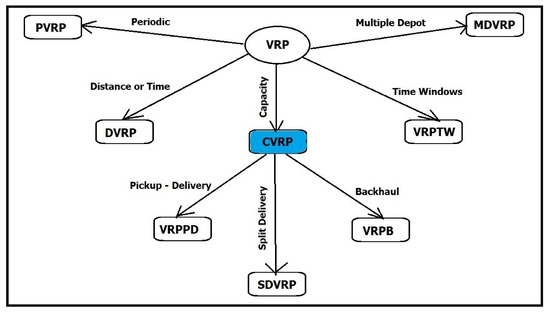
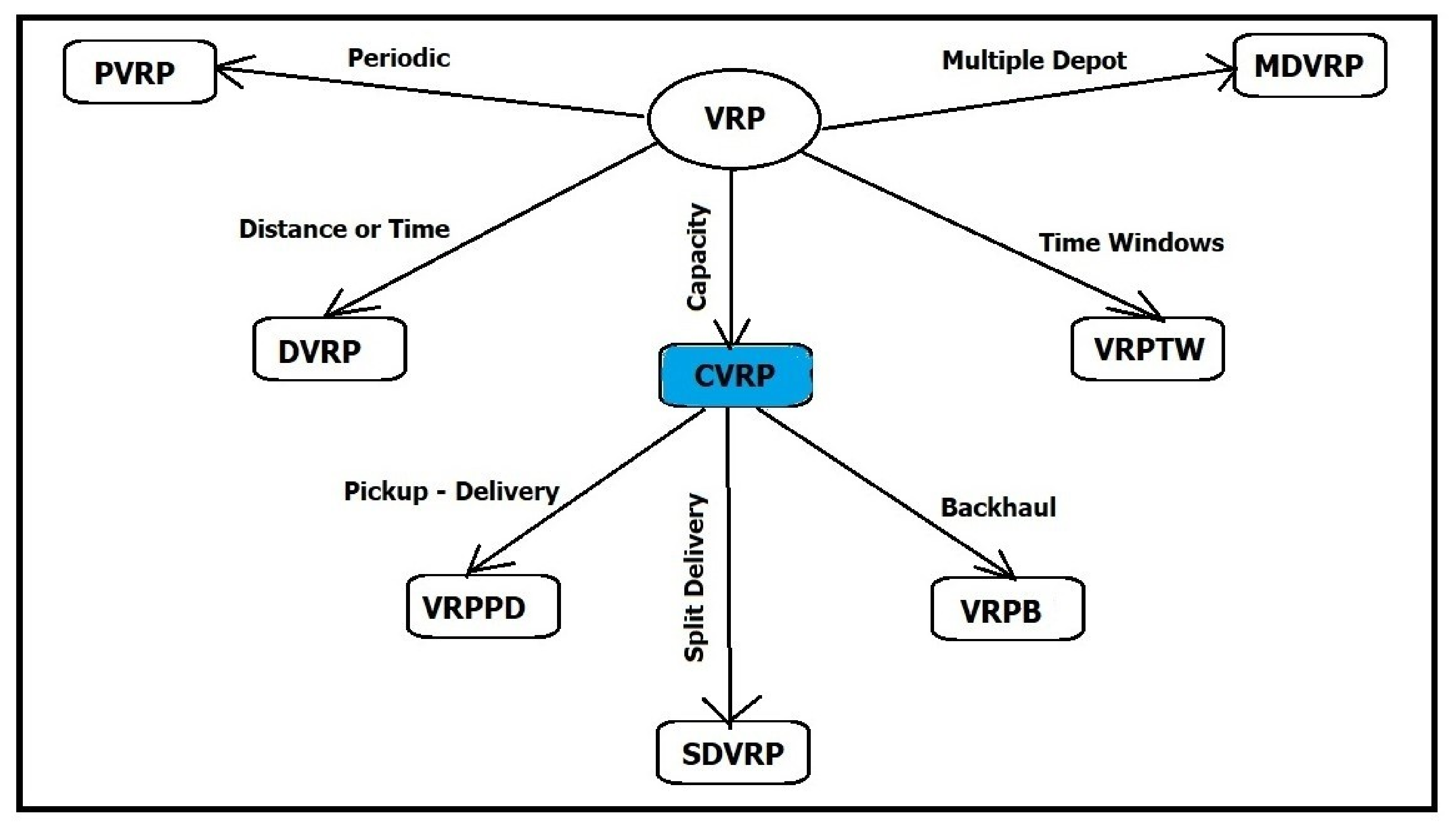
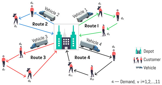
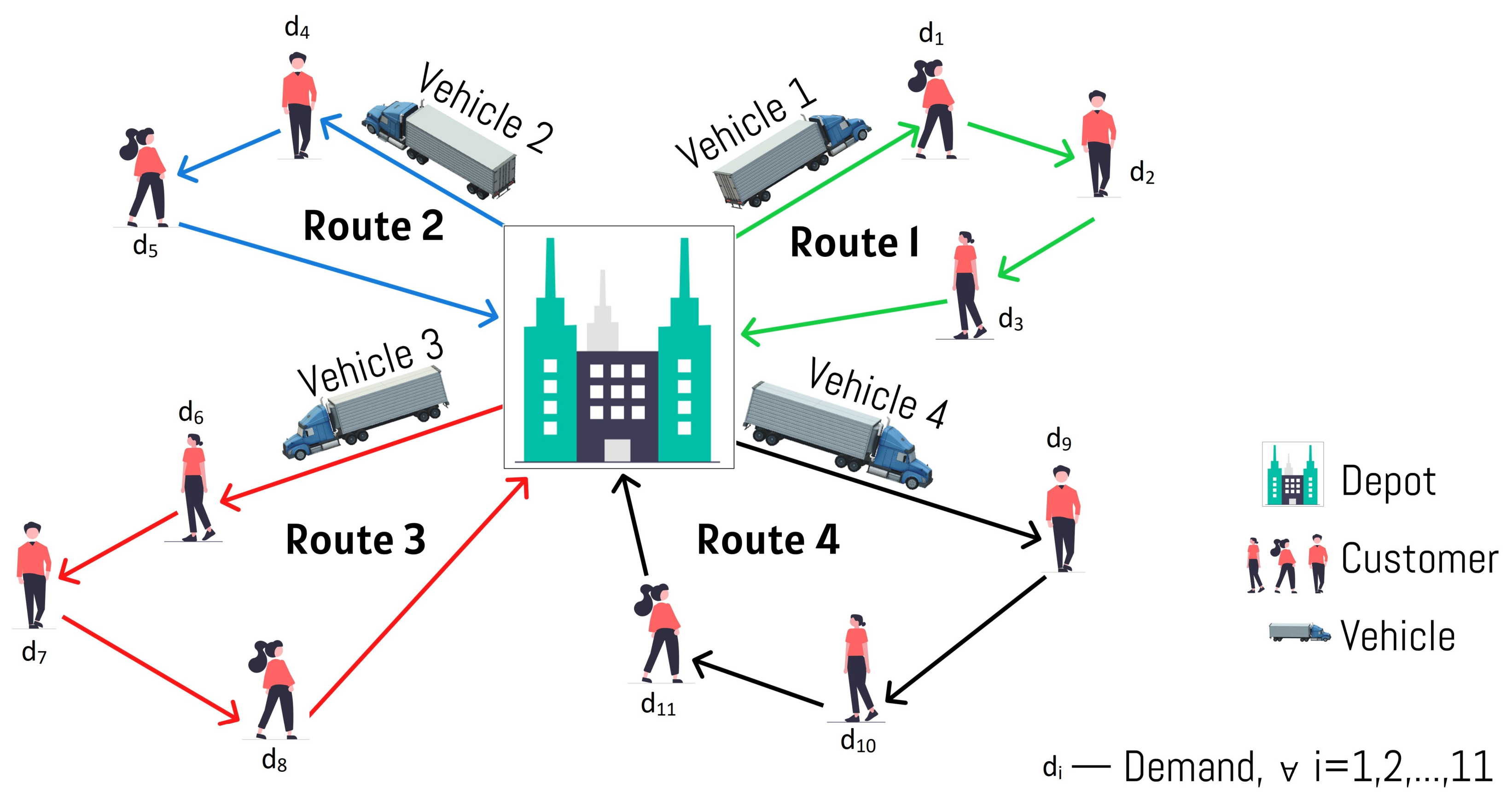
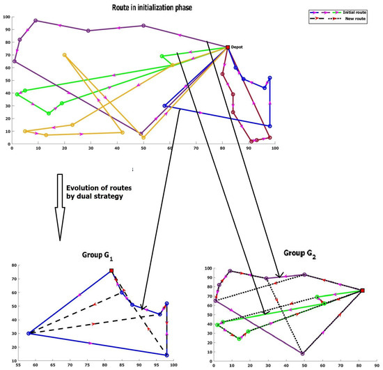
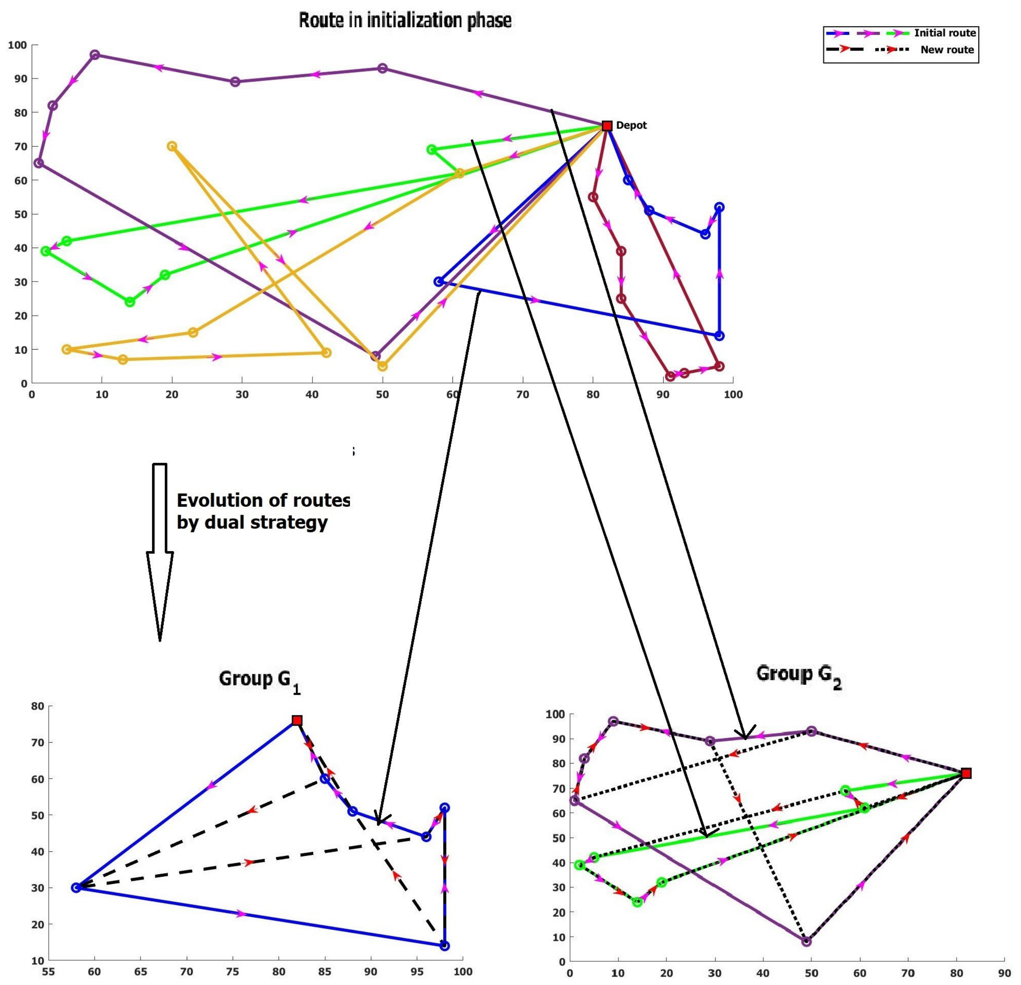
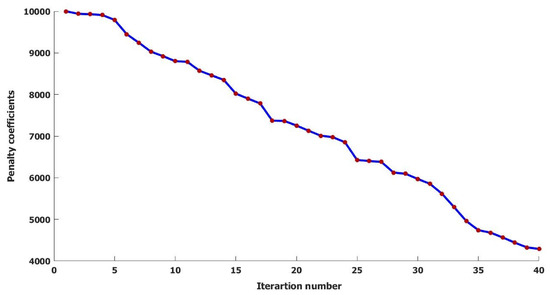
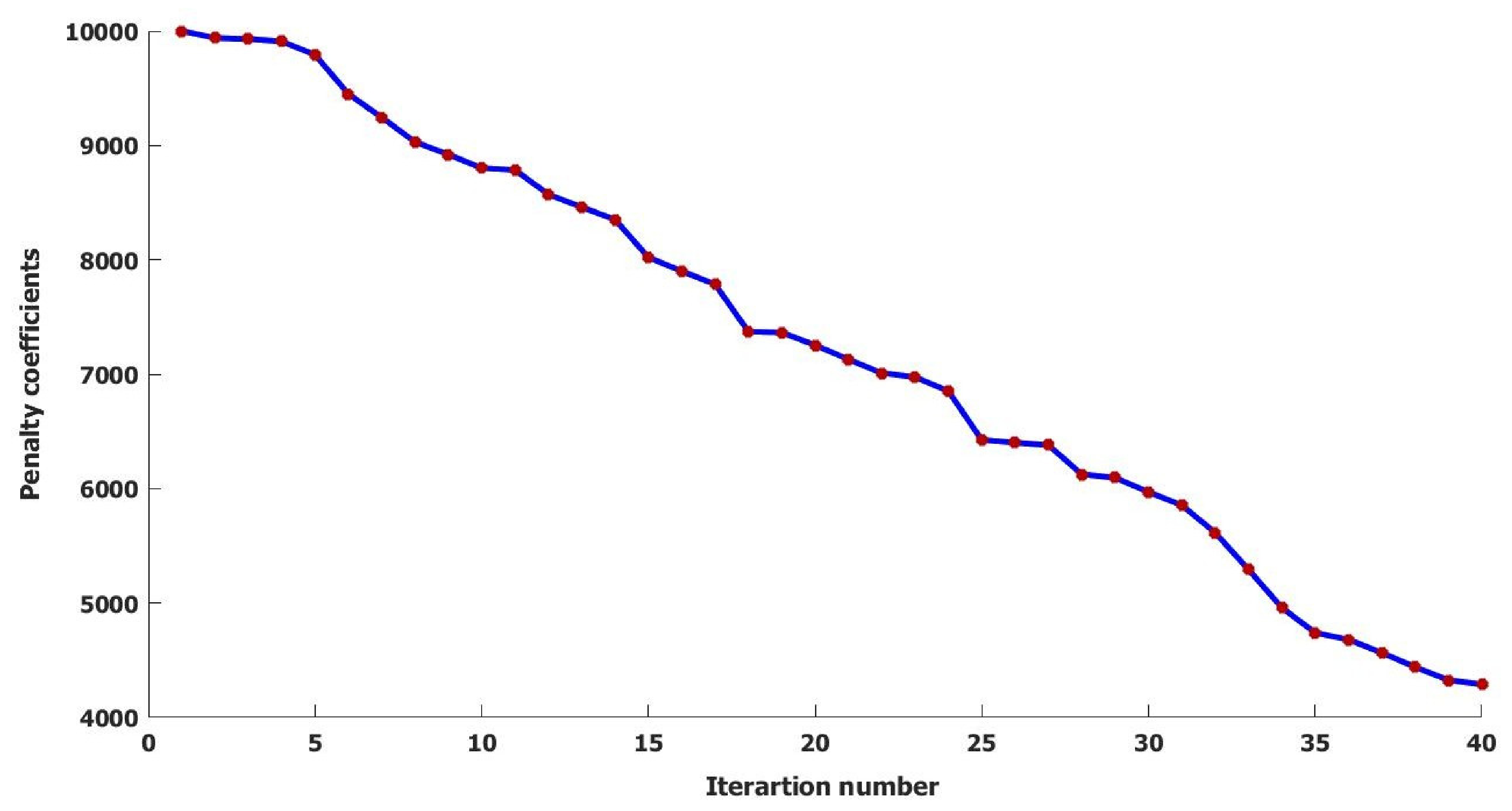
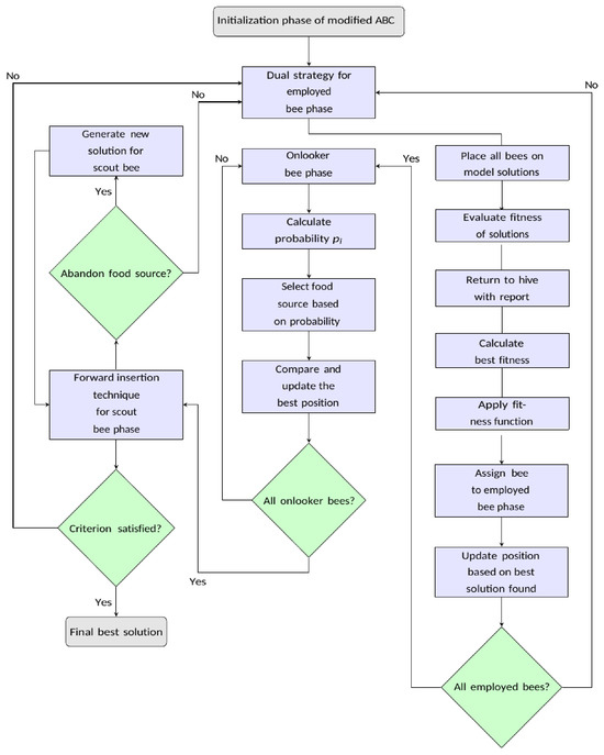
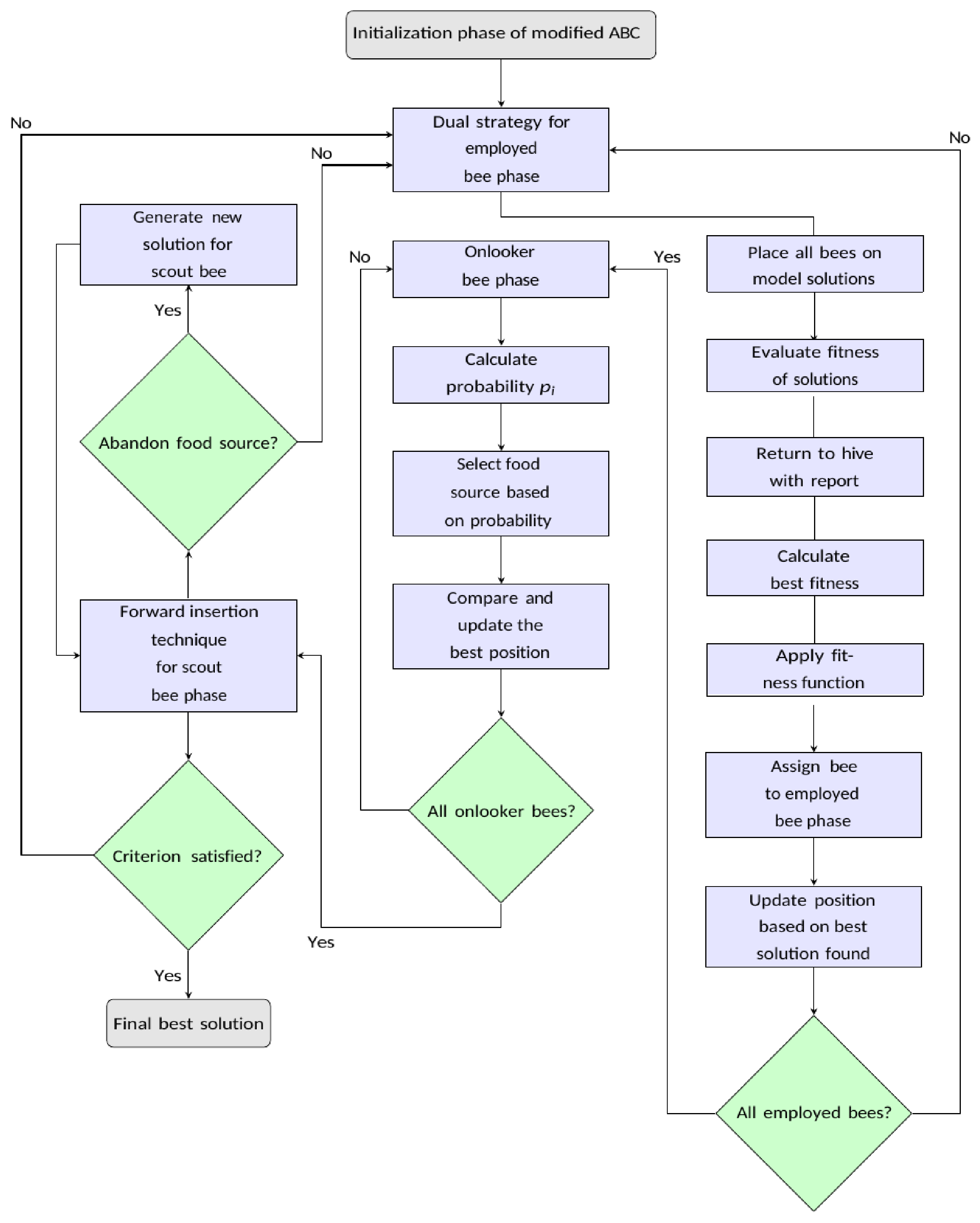
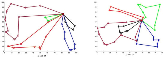
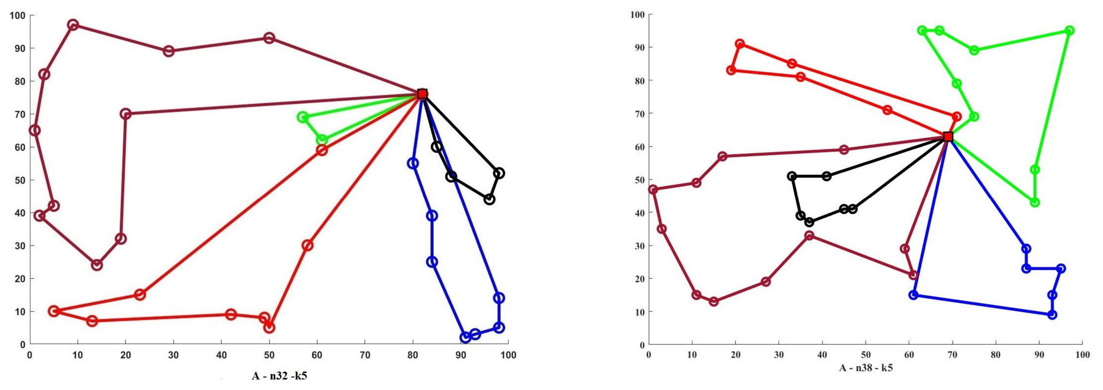
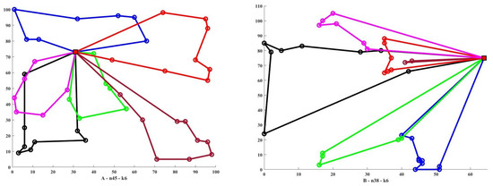
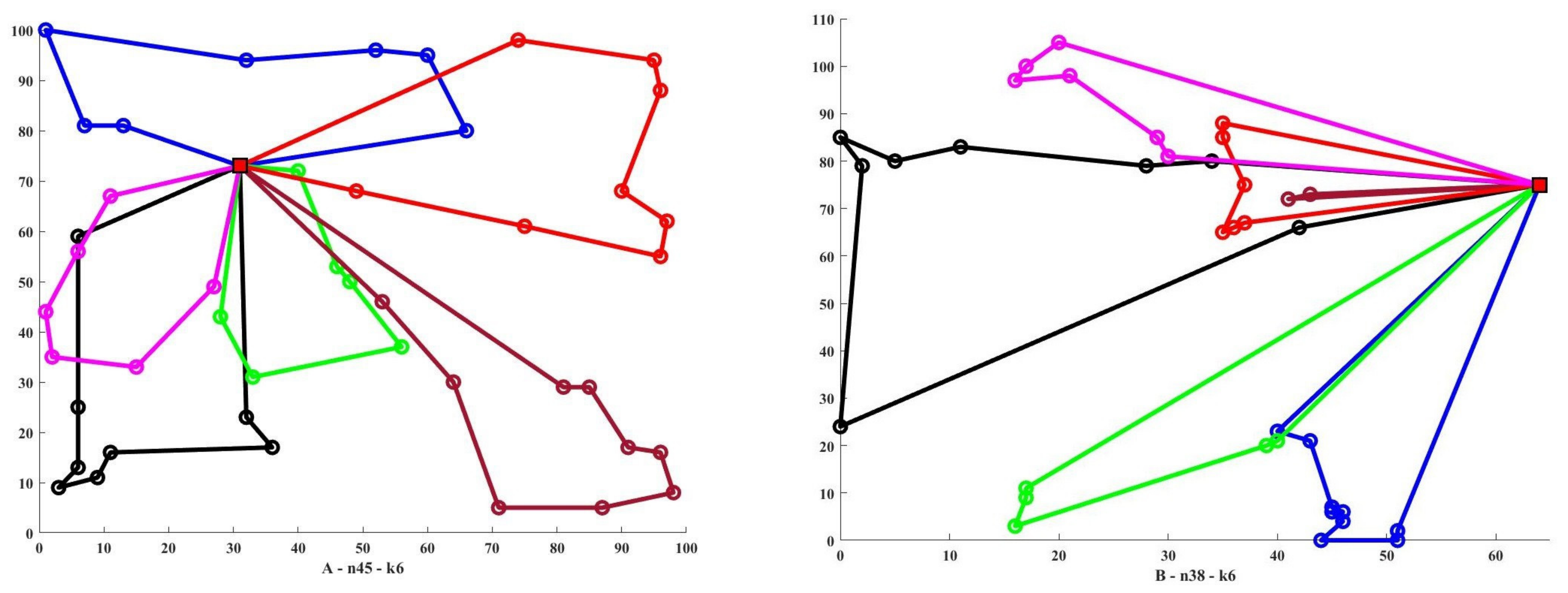

Disclaimer/Publisher’s Note: The statements, opinions and data contained in all publications are solely those of the individual author(s) and contributor(s) and not of MDPI and/or the editor(s). MDPI and/or the editor(s) disclaim responsibility for any injury to people or property resulting from any ideas, methods, instructions or products referred to in the content. |
© 2026 by the authors. Licensee MDPI, Basel, Switzerland. This article is an open access article distributed under the terms and conditions of the Creative Commons Attribution (CC BY) license.