Markov Cell Processes

Abstract

We define a class of Markov cell processes, $P_X$, on a finite set, X, as a product of conditional probabilities on cells (subsets of X forming a partially directed intersection graph). The class of Markov cell processes includes Bayesian networks and Markov edge processes. A nested conditional independence (NCI) condition is introduced that allows an explicit expression of a joint probability distribution through its marginals. The NCI condition is used in our construction of consistent Markov cell processes $P_X$ whose marginals coincide with $P_{X^{\prime }}$ on smaller sets $X^{\prime }\subset X$. We discuss three classes of consistent Markov cell processes on rectangular domains $X\subset {\mathbb{Z}}^3$ equipped with ‘cubic’ cells, which include the Arak model and 3D Pickard model.

1. Introduction

This work introduces a class of Markov cell processes, $Y_X=\{Y_x;x\in X\}$, on a finite set, X, with probability distribution $P_X\left(y_X\right)\equiv P(Y_x=y_x,x\in X)$ written as a product

$$\begin{array}{ccc}\hfill P_X\left(y_X\right)& =& \prod _{i\in K}{\pi }_i(y_{{\tilde{C}}_i^{-}}|y_{C_i^{-}}),\hfill \end{array}$$

(1)

of conditional (cell) probabilities ${\pi }_i(y_{{\tilde{C}}_i^{-}}|y_{C_i^{-}})$ on cells—subsets $C_i\subset X,i\in K=\{1,\cdots ,k\}$, rigorously defined in Section 2. Cells may intersect and are partially directed, with $C_i^{-}$ interpreted as the ‘past’ of $C_i$ and ${\tilde{C}}_i^{-}:=C_i\setminus C_i^{-}$. More specifically, cells form a partially directed acyclic intersection graph $\overrightarrow{H}\left(\mathcal{C}\right)=(V\left(\mathcal{C}\right),\overrightarrow{E}\left(\mathcal{C}\right))$ (called a cell graph in this paper), with the vertex set $V\left(\mathcal{C}\right)=\{C_i;i\in K\}$ and an edge set $\overrightarrow{E}\left(\mathcal{C}\right)$ of directed pairs $(C_i\to C_j),C_i\cap C_j\ne \varnothing ,i\ne j$. In the simplest case, $X=\{1,\cdots ,n,n+1\},C_i=\{i,i+1\},$ (1) is a Markov chain with transition probabilities ${\pi }_i\left(y_{i+1}\right|y_i)$, as shown in Remark 2, but the fact that $C_i$ in (1) may contain more than two elements of X gives rise to a large class of probability models used in networks, learning, image analysis, and other applied fields.

The notion of a cell graph is related to that of a directed hypergraph, providing a framework for modeling complex problems in operations research and computer science; see [1,2] and the references therein. A particular but very important case of a cell graph is the family cell graph, with cells formed by families at v (a vertex $v\in V$ of a directed acyclic graph (DAG) $\overrightarrow{G}=(V,\overrightarrow{E})$ and its parent vertices), in which case, Markov cell process in (1) agrees with the definition of Bayesian network (Example 2 below).

If the number $k=\left|K\right|$ of cells is large, (1) generally leads to a complicated probability distribution, depending on many parameters. In particular, finding the marginal distribution of $Y_x$ and the covariance function $\mathrm{Cov}(Y_x,Y_{x^{\prime }})$ for the given $x,x^{\prime }\in X$ may be very hard. Pickard [3,4] introduced a class of Bayesian networks $P_X$ (Markov random fields) on rectangular sets $X\subset {\mathbb{Z}}^2$ satisfying the consistency property: for any rectangles $X^{\prime }\subset X$,

$$P_{X|X^{\prime }}=P_{X^{\prime }}$$

(2)

where $P_{X|X^{\prime }}$ is the restriction in the marginal of $Y_X$ on $X^{\prime }$. Property (2) implies that the restrictions of the Pickard model on the horizontal and vertical lines are (stationary) Markov chains with explicit transition probabilities. Pickard random fields have been found to be useful in a number of applied fields [5,6,7,8,9,10]. Independently, Refs. [11,12] studied a class of polygonal Markov random fields with the continuous argument $x\in X\subset {\mathbb{R}}^2$ with a similar consistency property in (2), defined through the evolution of the one-dimensional particle system with random piece-wise constant Markov velocity, interacting at collisions. Recent work [13] investigated a class of Markov edge processes in the set $X=\overrightarrow{E}$ of edges of a DAG $\overrightarrow{G}=(V,\overrightarrow{E})$, satisfying the consistency relation in (2) with regard to $X^{\prime }\subset X$ obtained from $\overrightarrow{G}$ by a mesh-dismantling algorithm. We note that Markov edge processes are a particular case of Markov cell processes, in which case, cells $C_v$ are the set of edges incident to a given vertex $v\in V$, with $(C_v\to C_{v^{\prime }})\in \overrightarrow{E}\left(\mathcal{C}\right)$ equivalent to $(v\to v^{\prime })\in \overrightarrow{E}.$ In the case of the Pickard model, cells are unit squares of ${\mathbb{Z}}^2$ directed in the lexicographic order, cell distributions defined on quadruples $(y_A,y_B,y_C,y_D)$ indexed by four points of square; see Example 14.

Needless to say, the consistency property in the above models holds under strong additional conditions on cell distributions ${\pi }_i$ [4,5,8,13]. Our main result (Theorem 1 of Section 5) obtains sufficient conditions on cell graph $\overrightarrow{H}\left(\mathcal{C}\right)$ and distributions ${\pi }_i,i\in K$ in order such that a general Markov cell process in (1) satisfies the consistency property in (2) with respect to a class of cell subgraphs $\overrightarrow{H}\left({\mathcal{C}}^{\prime }\right)=(V\left({\mathcal{C}}^{\prime }\right),\overrightarrow{E}\left({\mathcal{C}}^{\prime }\right)),X^{\prime }=V\left({\mathcal{C}}^{\prime }\right)$ obtained from $\overrightarrow{H}\left(\mathcal{C}\right)$ by a cell dismantling algorithm (CDA). The central condition of Theorem 1 is Assumption 5, which relies on the concept of nested conditional independence (NCI), introduced in Section 4, and applicable to a general probability distribution $P_E\left(y_E\right)=P(y_e,e\in E)$ on a finite set E written as a union $E={\bigcup }_{r\in L}{E}_r$ of possibly intersecting sets $E_r,r\in L$, and involving marginals $P\left(y_{E\left(S\right)}\right)$ on intersections $E\left(S\right)={\bigcap }_{r\in S}{E}_r$. According to (factorization) Lemma 1, the NCI condition implies that $P_E$ is written as a product of its marginals as

$$P\left(y_E\right)=\prod _{\left|S\right|=1}P\left(y_{E\left(S\right)}\right){\displaystyle \frac{1}{{\prod }_{\left|S\right|=2}P\left(y_{E\left(S\right)}\right)\frac{1}{{\prod }_{\left|S\right|=3}P\left(y_{E\left(S\right)}\right)}\cdots }}$$

(3)

(the products on the r.h.s. of (3) terminate when $E\left(S\right)=\varnothing$ for $\left|S\right|$ large enough). In some cases (independent marginals, Markov chains), (3) is well-known or trivial, but, in the general case, (3) seems new in probability theory. We note that Assumption 5 (NCI^± conditions for ‘future’/‘past’ cell probabilities) agrees with the conditional and marginal independence conditions for Picard and Markov edge processes; see Examples 13 and 14. The last Section 6 is devoted to three classes of consistent Markov cell processes on ${\mathbb{Z}}^3$ indexed by faces, edges, or vertices of ‘cubic’ cells and referred to Models F, E, and V in this paper, which include the 3D Arak model and 3D Pickard model, focusing on the formulation and verification of NCI^± conditions for these models.

This paper introduces a new and general class of network models and dependence structures characterized by dependence between cells. The primary aim of this work is to develop and explain the underlying theoretical concepts and relate them to existing network models. Concrete applications of Markov cell processes is an open and non-trivial problem.

All probability distributions in our paper are discrete. Extensions to continuous (e.g., Gaussian) distributions seem feasible.

2. Definitions and Notation

Let X be a finite set and $\varnothing \ne C_i\subset X,i\in K:=\{1,\cdots ,k\}$ a given family of subsets of X called cells in this paper. W.l.g., we assume that

$$\bigcup _{i\in K}{C}_i=X.$$

Two cells, $C_i,C_j(i\ne j)$, are connected if

$$C_i\cap C_j\ne \varnothing .$$

Thus,

$$H\left(\mathcal{C}\right)=(V\left(\mathcal{C}\right),E\left(\mathcal{C}\right)),V\left(\mathcal{C}\right):=\{C_i,i\in K\},E\left(\mathcal{C}\right):=\{(C_i,C_j):i,j\in K,i\ne j,C_i\cap C_j\ne \varnothing \}$$

(4)

is a graph with the vertex set $V\left(\mathcal{C}\right)$ composed of all cells $C_i$ and the edge set $E\left(\mathcal{C}\right)$ consisting of connected pairs $(C_i,C_j)$ of cells.

We next postulate that some edges in $E\left(\mathcal{C}\right)$ are directed, with

$$\overrightarrow{E}\left(\mathcal{C}\right):=\{(C_i\to C_j):(C_i,C_j)\in E\left(\mathcal{C}\right),i,j\in K\}$$

standing for the set of directed edges. The corresponding directed graph is denoted by

$$\overrightarrow{H}\left(\mathcal{C}\right):=(V\left(\mathcal{C}\right),\overrightarrow{E}\left(\mathcal{C}\right)).$$

(5)

Following the terminology of kinship in directed networks, we call $C_j$ in $(C_i\to C_j)\in E\left(\mathcal{C}\right)$ the child cell, and $C_i$ the parent cell.

Assumption 1.

The directed graph in (5) is acyclic (DAG).

We introduce the following terminology distinguishing graphical objects used in the construction of Markov cell process.

Definition 1.

A cell graph is a partially directed intersection graph, $\overrightarrow{H}\left(\mathcal{C}\right)$, in (5). A cell DAG is a cell graph satisfying Assumption 1.

We denote ⪯, the partial order relation in $\overrightarrow{H}\left(\mathcal{C}\right)$, viz., $C^{\prime }\prec C^{″}$ whenever $(C^{\prime }\to C^{″})\in \overrightarrow{E}\left(\mathcal{C}\right)$ or there is a directed path $(C^{\prime }\to C_1)\in \overrightarrow{E}\left(\mathcal{C}\right),(C_1\to C_2)\in \overrightarrow{E}\left(\mathcal{C}\right),\cdots ,(C_{\mathcal{l}}\to C^{″})\in \overrightarrow{E}\left(\mathcal{C}\right),\cdots ,(\mathcal{l}\ge 1)$. For a given cell DAG $\overrightarrow{H}\left(\mathcal{C}\right)=(V\left(\mathcal{C}\right),\overrightarrow{E}\left(\mathcal{C}\right)$ in (5) and a given cell $C_i\in V\left(\mathcal{C}\right)$ introduce the notation,

$$\begin{array}{ccc}\hfill C_i^{-}& :=& \{x\in C_i\cap C_j:\exists (C_j\to C_i)\in \overrightarrow{E}\left(\mathcal{C}\right)\},{\tilde{C}}_i^{-}:=C_i\setminus C_i^{-}.\hfill \end{array}$$

(6)

We shall refer to $C_i^{-}$ as the past (part) of cell $C_i$. Symmetric notions $C_i^{+}:=\{x\in C_i\cap C_j:\exists (C_i\to C_j)\in \overrightarrow{E}\left(\mathcal{C}\right)\},$ (the future (part) of $C_i$), ${\tilde{C}}_i^{+}:=C_i\setminus C_i^{+}$ are analogs of (6) for the reversed cell DAG

$$\begin{array}{c}\overleftarrow{H}\end{array}\left(\mathcal{C}\right):=(V\left(\mathcal{C}\right),\begin{array}{c}\overleftarrow{E}\end{array}\left(\mathcal{C}\right)),(C_i\leftarrow C_j)\in \begin{array}{c}\overleftarrow{E}\end{array}\left(\mathcal{C}\right)⟺(C_j\to C_i)\in \overrightarrow{E}\left(\mathcal{C}\right),i,j\in K.$$

(7)

Assumption 2.

For any cells $C_i,C_j,i\ne j$,

$${\tilde{C}}_i^{+}\cap C_j\ne \varnothing ⟹(C_j\to C_i)\in \overrightarrow{E}\left(\mathcal{C}\right)$$

Assumption 3.

For any cells $C_i,C_j,i\ne j$,

$${\tilde{C}}_i^{-}\cap C_j\ne \varnothing ⟹(C_i\to C_j)\in \overrightarrow{E}\left(\mathcal{C}\right)$$

(8)

A cell $C_i$ is called a source cell if $C_i^{-}=\varnothing$, and a sink cell if $C_i^{+}=\varnothing$. Assumption 3 implies that two source cells $C_i,C_j$ are disconnected: $C_i\cap C_j=\varnothing$ since, otherwise, by (8), it follows that $(C_i\to C_j)\in \overrightarrow{E}\left(\mathcal{C}\right)$ and $(C_j\to C_i)\in \overrightarrow{E}\left(\mathcal{C}\right)$ which is not possible. Similarly, Assumption 2 implies that two sink cells $C_i,C_j$ do not intersect.

In the following examples, X is the set of vertices or edges of a DAG $\overrightarrow{G}=(V,\overrightarrow{E})$ and cells are subsets of X indexed by $v\in V.$

Example 1

(Edge cells). Let $\overrightarrow{G}=(V,\overrightarrow{E})$ be a DAG with vertex set V and a set $\overrightarrow{E}$ of directed edges $e=(v^{\prime }\to v),v,v^{\prime }\in V,v\ne v^{\prime }.$ The set of edges incident to a $v\in V$, viz.,

$$C_v:=\{e=(v\to v^{\prime })\in \overrightarrow{E},v^{\prime }\in V\}\cup \{e=(v^{\prime }\to v)\in \overrightarrow{E},v^{\prime }\in V\}$$

(9)

form the edge clique at v (i.e., a clique in the line graph ${\overrightarrow{G}}_E=(V\left(G_E\right),\overrightarrow{E}\left(G_E\right))$ of $\overrightarrow{G}$. The set $V\left(\mathcal{C}\right):=\{C_v;v\in V\}$ of all edge cliques with $E\left(\mathcal{C}\right)=\{(C_v,C_{v^{\prime }}):C_v\cap C_{v^{\prime }}\ne \varnothing ,v,v^{\prime }\in V,v\ne v^{\prime }\}$ is a graph $H\left(\mathcal{C}\right)=\left(V\right(\mathcal{C}),E(\mathcal{C}\left)\right)$ which can be directed following the underlying graph $\overrightarrow{G}$:

$$(C_v\to C_{v^{\prime }})\in \overrightarrow{E}\left(\mathcal{C}\right)⟺(v\to v^{\prime })\in \overrightarrow{E}.$$

(10)

Since $C_v\cap C_{v^{\prime }}\ne \varnothing$ implies either $(v\to v^{\prime })\in \overrightarrow{E}$ or $(v^{\prime }\to v)\in \overrightarrow{E}$, all connected sets are directed. Note also

$$\begin{array}{c}\hfill C_v^{-}=\{e=(v^{\prime }\to v)\in \overrightarrow{E}\},{\tilde{C}}_v^{-}=\{e=(v\to v^{\prime })\in \overrightarrow{E}\}\end{array}$$

(11)

are the sets of incoming and outgoing edges incident to v. It is easy to see that the above $\overrightarrow{H}\left(\mathcal{C}\right)$ satisfies Assumptions 1, 2 and 3.

Example 2

(Family cells). Let $\overrightarrow{G}=(V,\overrightarrow{E})$ be the same as in Example 1 and let

$$C_v:=\left\{v\right\}\cup \mathrm{pa}\left(v\right),\mathrm{pa}\left(v\right):=\{v^{\prime }\in V:(v^{\prime }\to v)\in \overrightarrow{E}\}.$$

(12)

The set $C_v$ in (12) is called the family at v, consisting of v and the set $\mathrm{pa}\left(v\right)$ of parents of v. A family cell DAG $\overrightarrow{H}\left(\mathcal{C}\right)=(V\left(\mathcal{C}\right),\overrightarrow{E}\left(\mathcal{C}\right))$ is a cell DAG with $V\left(\mathcal{C}\right)=\{C_v;v\in V\}$ and edges

$$(C_v\to C_{v^{\prime }})\in \overrightarrow{E}\left(\mathcal{C}\right)⟺(v\to v^{\prime })\in \overrightarrow{E},$$

which agree with edges of $\overrightarrow{G}$. We have

$$\begin{array}{c}\hfill C_v^{-}=\mathrm{pa}\left(v\right),{\tilde{C}}_v^{-}=\left\{v\right\},\end{array}$$

(13)

Note that the above $\overrightarrow{H}\left(\mathcal{C}\right)$ satisfies Assumptions 1 and 3, but does not satisfy Assumption 2 in general.

Example 3

(Interval cells). Let $\overrightarrow{G}=(V,\overrightarrow{E})$ be as in Examples 1 and 2, with the partial order relation $v⪯v^{\prime }$. A set

$$V_{[v_{-},v_{+}]}:=\{v\in V:v_{-}⪯v⪯v_{+}\}$$

(14)

is called interval, with the convention that $V_{[v,v]}=\left\{v\right\}$ and $V_{[v_{-},v_{+}]}=\varnothing$ when the r.h.s. of (14) is empty (that is, when $v_{+}$ is not reachable from $v_{-}$). The class of intervals and the corresponding cells

$$C_{[v_{-},v_{+}]}=\{e=(v_1\to v_2)\in \overrightarrow{E},v_1,v_2\in V_{[v_{-},v_{+}]}\}$$

(15)

is very large and indexed by two vertices $v_{\pm }$, in contrast to Examples 1 and 2. Directed edges between two interval cells can be introduced as

$$(C_{[v_{-},v_{+}]}\to C_{[v_{-}^{\prime },v_{+}^{\prime }]})⟺v_{-}\prec v_{-}^{\prime }\prec v_{+}\prec v_{+}^{\prime }.\mathit{and}C\left(v^{\prime }\right)\cap C\left(v\right)\ne \varnothing .$$

(16)

Apparently, there are many ways to define interval cell DAGs $\overrightarrow{H}\left(\mathcal{C}\right)=(V\left(\mathcal{C}\right),\overrightarrow{E}\left(\mathcal{C}\right))$ by choosing a set $V\left(\mathcal{C}\right)$ of interval cells with directed edges according to (16). Interval cell DAGs naturally arise on regular lattices, as shown in Example 14 (Pickard model) on ${\mathbb{Z}}^2$ and Model V on ${\mathbb{Z}}^3$ of Section 6.

Cell Dismantling Algorithm (CDA)

Given a cell DAG $\overrightarrow{H}\left(\mathcal{C}\right)=(V\left(\mathcal{C}\right),\overrightarrow{E}\left(\mathcal{C}\right))$ and a (nonempty) subset $V^{\prime }\subset V\left(\mathcal{C}\right)$, we define a cell subDAG

$$\overrightarrow{H}\left({\mathcal{C}}^{\prime }\right)=(V\left({\mathcal{C}}^{\prime }\right),\overrightarrow{E}\left({\mathcal{C}}^{\prime }\right))$$

(17)

with vertex set $V\left({\mathcal{C}}^{\prime }\right):=V^{\prime }$ and edge set $\overrightarrow{E}\left({\mathcal{C}}^{\prime }\right):=\{(C_i\to C_j)\in \overrightarrow{E}\left(\mathcal{C}\right):C_i,C_j\in V^{\prime }\}.$ Note (17) preserves Assumption 1; in other words, $\overrightarrow{H}\left({\mathcal{C}}^{\prime }\right)$ is a cell DAG for any subset $V^{\prime }\subset V\left(\mathcal{C}\right).$ The class of all cell subDAGs in (17) is denoted $\mathcal{S}\left(\overrightarrow{H}\left(\mathcal{C}\right)\right)$. The following definition of CDA is similar to that of MDA (mesh dismantling algorithm) ([13] [Definition 4]).

Definition 2.

A transformation $\overrightarrow{H}\left(\mathcal{C}\right){\to }_{+}\overrightarrow{H}\left({\mathcal{C}}^{\prime }\right)\in \mathcal{S}\left(\overrightarrow{H}\left(\mathcal{C}\right)\right)$ is said a top cell dismantling algorithm (top CDA) if it removes a sink cell, in other words, if $V\left({\mathcal{C}}^{\prime }\right)=V\left(\mathcal{C}\right)\setminus \left\{C_r\right\}$, where $C_r$ is a sink cell.

Similarly, $\overrightarrow{H}\left(\mathcal{C}\right){\to }_{+}\overrightarrow{H}\left({\mathcal{C}}^{\prime }\right)\in \mathcal{S}\left(\overrightarrow{H}\left(\mathcal{C}\right)\right)$ is said to be a bottom cell dismantling algorithm (bottom CDA) if it removes a source cell, in other words, if $V\left({\mathcal{C}}^{\prime }\right)=V\left(\mathcal{C}\right)\setminus \left\{C_r\right\}$, where $C_r$ is a source cell.

We denote ${\mathcal{S}}_{\mathrm{CDA}}^{+}\left(\overrightarrow{H}\left(\mathcal{C}\right)\right)$, ${\mathcal{S}}_{\mathrm{CDA}}^{-}\left(\overrightarrow{H}\left(\mathcal{C}\right)\right)$, ${\mathcal{S}}_{\mathrm{CDA}}\left(\overrightarrow{H}\left(\mathcal{C}\right)\right)$ as the classes of cell subDAGs in (17) which can be obtained from $\overrightarrow{H}\left(\mathcal{C}\right)$ by succesively applying a top CDA, bottom CDA, or both types of CDA in an arbitrary order:

$$\begin{array}{ccc}\hfill {\mathcal{S}}_{\mathrm{CDA}}^{+}\left(\overrightarrow{H}\left(\mathcal{C}\right)\right)& :=& \left\{\overrightarrow{H}\left(\mathcal{C}\right)\right\}\cup \{\overrightarrow{H}\left({\mathcal{C}}^{\prime }\right)=\overrightarrow{H}\left({\mathcal{C}}_i^{\prime }\right),i\ge 1\},\overrightarrow{H}\left(\mathcal{C}\right){\to }_{+}\overrightarrow{H}\left({\mathcal{C}}_1^{\prime }\right){\to }_{+}\cdots {\to }_{+}\overrightarrow{H}\left({\mathcal{C}}_i^{\prime }\right),\hfill \\ \hfill {\mathcal{S}}_{\mathrm{CDA}}^{-}\left(\overrightarrow{H}\left(\mathcal{C}\right)\right)& :=& \left\{\overrightarrow{H}\left(\mathcal{C}\right)\right\}\cup \{\overrightarrow{H}\left({\mathcal{C}}^{\prime }\right)=\overrightarrow{H}\left({\mathcal{C}}_i^{\prime }\right),i\ge 1\},\overrightarrow{H}\left(\mathcal{C}\right){\to }_{-}\overrightarrow{H}\left({\mathcal{C}}_1^{\prime }\right){\to }_{-}\cdots {\to }_{-}\overrightarrow{H}\left({\mathcal{C}}_i^{\prime }\right),\hfill \\ \hfill {\mathcal{S}}_{\mathrm{CDA}}\left(\overrightarrow{H}\left(\mathcal{C}\right)\right)& :=& \left\{\overrightarrow{H}\left(\mathcal{C}\right)\right\}\cup \{\overrightarrow{H}\left({\mathcal{C}}^{\prime }\right)=\overrightarrow{H}\left({\mathcal{C}}_i^{\prime }\right),i\ge 1\},\overrightarrow{H}\left(\mathcal{C}\right){\to }_{\pm }\overrightarrow{H}\left({\mathcal{C}}_1^{\prime }\right){\to }_{\pm }\cdots {\to }_{\pm }\overrightarrow{H}\left({\mathcal{C}}_i^{\prime }\right).\hfill \end{array}$$

Proposition 1.

Let $\overrightarrow{H}\left(\mathcal{C}\right)$ satisfy Assumption 3 (respectively, Assumption 2) and $\overrightarrow{H}\left({\mathcal{C}}^{\prime }\right)\in {\mathcal{S}}_{\mathrm{CDA}}^{+}$ ($\overrightarrow{H}\left({\mathcal{C}}^{\prime }\right)\in {\mathcal{S}}_{\mathrm{CDA}}^{-}$, respectively). Then, $\overrightarrow{H}\left({\mathcal{C}}^{\prime }\right)$ satisfies Assumption 3 (respectively, Assumption 2).

Proof. 

It suffices to show the proposition for one step top CDA and $\overrightarrow{H}\left(\mathcal{C}\right)$ satisfying Assumption 3. Let $V\left(\mathcal{C}\right)=\{C_1,\cdots ,C_k\}$, $C_k$ be a sink cell, $C_k^{+}=\varnothing ,$ and $\overrightarrow{H}\left({\mathcal{C}}^{\prime }\right)$ be as in (17), with $V^{\prime }=V\left({\mathcal{C}}^{\prime }\right)=V\left(\mathcal{C}\right)\setminus \left\{C_k\right\}=\{C_1,\cdots ,C_{k-1}\}.$ For $i\le k-1$,

$$C_i^{-}={\bigcup }_{1\le j\le k:(C_j\to C_i)\in \overrightarrow{E}\left(\mathcal{C}\right)}{C}_j\cap C_i={\bigcup }_{1\le j\le k-1:(C_j\to C_i)\in \overrightarrow{E}\left(\mathcal{C}\right)}{C}_j\cap C_i$$

since $(C_k\to C_i)\notin \overrightarrow{E}\left(\mathcal{C}\right),$ $C_k$ being a cell sink. By Assumption 3, ${\tilde{C}}_i^{-}\cap C_j\ne \varnothing$ implies $(C_i\to C_j)\in \overrightarrow{E}\left(\mathcal{C}\right)$ for any $1\le i,j\le k,i\ne j$, hence also for $1\le i,j\le k-1,i\ne j$. Therefore, $\overrightarrow{H}\left({\mathcal{C}}^{\prime }\right)$ also satisfies Assumption 3. □

3. Markov Cell Process

Definition 3.

Let $H\left(\mathcal{C}\right)=\left(V\right(\mathcal{C}),E(\mathcal{C})$ be a cell graph in (4). A cell process on $H\left(\mathcal{C}\right)$ is a random process $Y_{C_i}=\{Y_{C_i};C_i\in V\left(\mathcal{C}\right),i\in K\}$ indexed by cells $C_i\in V\left(\mathcal{C}\right)$ and taking (vector) values

$$Y_{C_i}=(Y_{C_i}\left(x\right),x\in C_i),C_i\in V\left(\mathcal{C}\right)$$

which satisfies the following compatibility condition: for any cells, $(C_i,C_j)\in E\left(\mathcal{C}\right),i,j\in K$

$$Y_{C_i}\left(x\right)=Y_{C_j}\left(x\right),\forall x\in C_i\cap C_j.$$

(18)

Remark 1.

Observably, any cell process $Y_{C_i}=\{Y_{C_i};C_i\in V\left(\mathcal{C}\right)\}$ uniquely defines a scalar-valued process $Y_X=\{Y_x;x\in X\}$ by

$$Y_x:=Y_{C_i}\left(x\right),x\in X$$

for $C_i\in V\left(\mathcal{C}\right),i\in K$ since the last definition does not depend on i in view of (18).

A cell distribution on $C_i\in V\left(\mathcal{C}\right)$ is any (discrete) probability distribution ${\pi }_i\left(y_{C_i}\right)=\pi (y_x,x\in C_i)$ on the set of cell configurations $y_{C_i}=(y_x,x\in C_i)$. The conditional probabilities

$${\pi }_i(y_{{\tilde{C}}_i^{\pm }}|y_{C_i^{\pm }})={\displaystyle \frac{{\pi }_i\left(y_{C_i}\right)}{{\pi }_i(y_{C_i^{\pm }})}}$$

(19)

are defined in the usual way, with the convention that

$${\pi }_i(y_{{\tilde{C}}_i^{\pm }}|y_{C_i^{\mp }})=\left\{\begin{array}{cc}{\pi }_i\left(y_{C_i}\right),\hfill & C_i^{\pm }=\varnothing ,\hfill \\ 1,\hfill & {\tilde{C}}_i^{\pm }=\varnothing .\hfill \end{array}\right.$$

(20)

Definition 4.

Let $\overrightarrow{H}\left(\mathcal{C}\right)=(V\left(\mathcal{C}\right),\overrightarrow{E}\left(\mathcal{C}\right))$ be a cell DAG satisfying Assumption 3 and $\{{\pi }_i,i\in K\}$ be a family of cell distributions. A Markov cell process on $\overrightarrow{H}\left(\mathcal{C}\right)$ is a random process $Y=\{Y_x,x\in X\}$ s.t.

$$\begin{array}{ccc}\hfill P_X\left(y_X\right)\equiv P(Y_x=y_x,x\in X)& :=& \prod _{i\in K}{\pi }_i\left(y_{{\tilde{C}}_i^{-}}\right|y_{C_i^{-}}),\hfill \end{array}$$

(21)

where the product is taken over all cells $C_i\in V\left(\mathcal{C}\right)$.

Analogously, a Markov cell process $\widehat{Y}=\{{\widehat{Y}}_x,x\in X\}$ on the reversed cell DAG $\begin{array}{c}\overleftarrow{H}\end{array}\left(\mathcal{C}\right)=(V\left(\mathcal{C}\right),\begin{array}{c}\overleftarrow{E}\end{array}\left(\mathcal{C}\right))$ in (7) (corresponding to the same $\{{\pi }_i,i\in K\}$ as in (21)) is defined by

$$\begin{array}{ccc}\hfill {\widehat{P}}_X\left(y_X\right)\equiv \mathrm{P}({\widehat{Y}}_x=y_x,x\in X)& :=& \prod _{i\in K}{\pi }_i\left(y_{{\tilde{C}}_i^{+}}\right|y_{C_i^{+}}),\hfill \end{array}$$

(22)

where Assumption 3 is replaced by Assumption 2.

Proposition 2.

$P_X,{\widehat{P}}_X$ in (21), (22) are probability measures.

Proof. 

It suffices to prove the statement for $P_X$ alone. We use induction in $k=\left|K\right|$ (the number of cells). Clearly, the statement is true for $k=1$; we prove the induction step $k-1\to k$ as follows. Let $C_k$ be a cell sink of $\overrightarrow{H}\left(\mathcal{C}\right),$ then ${\tilde{C}}_k^{-}\cap {\cup }_{i=1}^{k-1}{C}_i=\varnothing ,X^{\prime }:=X\setminus {\tilde{C}}_k^{-}={\cup }_{i=1}^{k-1}{C}_i$ by Assumption 3, see the proof of Proposition 1, and

$$\begin{array}{ccc}\hfill \sum _{y_{{\tilde{C}}_k^{-}}}{P}_X\left(y_X\right)& =& {\displaystyle \prod _{i=1}^{k-1}}{\pi }_i\left(y_{{\tilde{C}}_i^{-}}\right|y_{C_i^{-}})\sum _{y_{{\tilde{C}}_k^{-}}}{\pi }_k\left(y_{{\tilde{C}}_k^{-}}\right|y_{C_k^{-}})={\displaystyle \prod _{i=1}^{k-1}}{\pi }_i\left(y_{{\tilde{C}}_i^{-}}\right|y_{C_i^{-}})=:P_{X^{\prime }}\left(y_{X^{\prime }}\right)\hfill \end{array}$$

(23)

is a Markov cell process on the cell subDAG $\overrightarrow{H}\left({\mathcal{C}}^{\prime }\right)=(V\left({\mathcal{C}}^{\prime }\right),\overrightarrow{E}\left({\mathcal{C}}^{\prime }\right))$ containing $k-1$ cells $V\left({\mathcal{C}}^{\prime }\right)=\{C_i,i\in K^{\prime }\},K^{\prime }=\{1,\cdots ,k-1\}$ and $\overrightarrow{E}\left({\mathcal{C}}^{\prime }\right)=\{(C_i\to C_j)\in \overrightarrow{E}\left(\mathcal{C}\right):C_i,C_j\in V\left({\mathcal{C}}^{\prime }\right)\}.$ Since $|K^{\prime }|=k-1<k,$ the induction assumption applies to $P_{X^{\prime }}$, implying the induction step $k-1\to k$. □

Example 4.

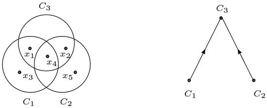
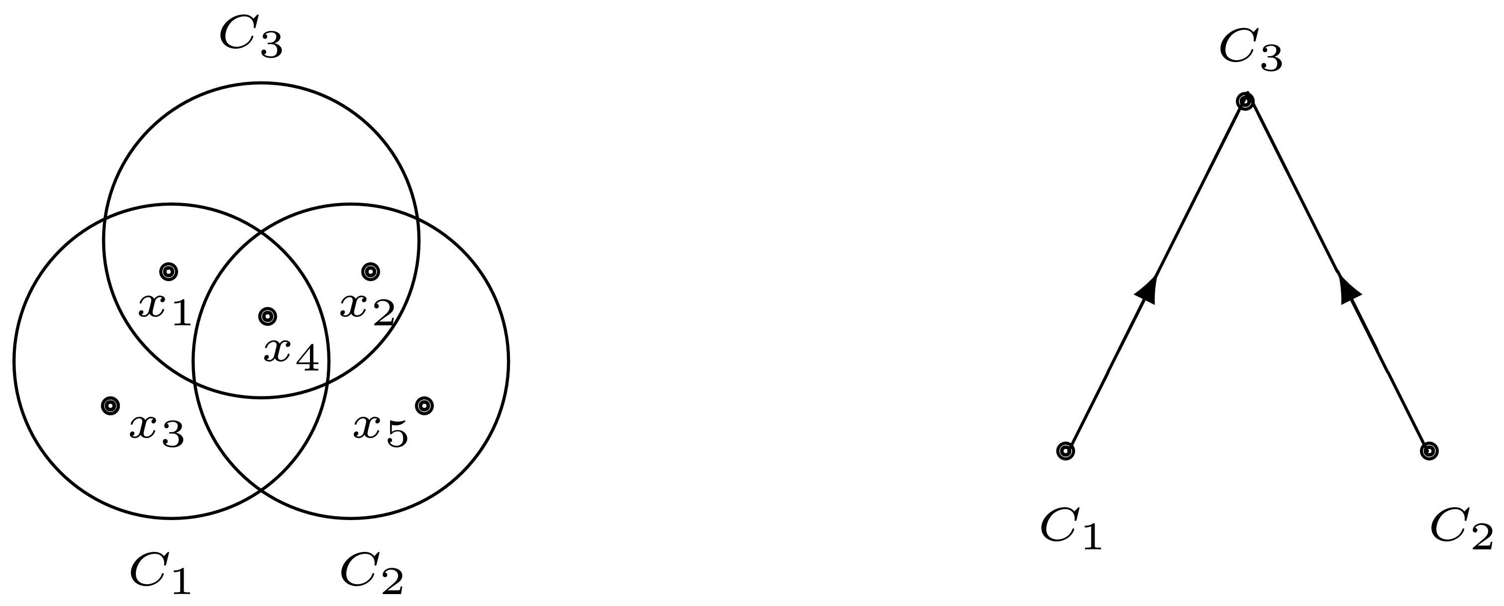
The following example of cell DAG (see Figure 1) shows that Assumption 3 is essential for Proposition 2. Namely, if Assumption 3 is dropped, the r.h.s. of (21) need not be a probability measure. Let $X=\{x_1,x_2,x_3,x_4,x_5\}$ consist of 5 points, and the graph $\overrightarrow{H}\left(\mathcal{C}\right)=(V\left(\mathcal{C}\right),\overrightarrow{E}\left(\mathcal{C}\right))$, $V\left(\mathcal{C}\right)=\{C_1,C_2,C_3\}$ consist of 3 cells as follows:

$$\begin{array}{c}\hfill C_1=\{x_1,x_3,x_4\},C_2=\{x_2,x_4,x_5\},C_3=\{x_1,x_2,x_4\},\overrightarrow{E}\left(\mathcal{C}\right)=\{(C_1\to C_3),(C_2\to C_3)\}\end{array}$$

Then ${\tilde{C}}_3^{-}=\varnothing ,{\tilde{C}}_1^{-}=C_1,{\tilde{C}}_2^{-}=C_2$ and $C_1\cap C_2={\tilde{C}}_1^{-}\cap C_2=C_1\cap {\tilde{C}}_2^{-}=\left\{x_4\right\}\ne \varnothing$ so that Assumption 3 is not fulfilled. Then,

$$\begin{array}{c}\hfill {\displaystyle \prod _{i=1}^3}{\pi }_i(y_{{\tilde{C}}_i^{-}}|y_{C_i^{-}})={\displaystyle \prod _{i=1}^2}{\pi }_i\left(y_{C_i}\right)={\pi }_1(y_{x_1},y_{x_3},y_{x_4}){\pi }_2(y_{x_2},y_{x_4},y_{x_5})\end{array}$$

is not a probability distribution since ${\sum }_{y_{x_1},y_{x_2},y_{x_3},y_{x_4}}{\prod }_{i=1}^2{\pi }_i\left(y_{C_i}\right)={\pi }_1\left(y_{x_4}\right){\pi }_2\left(y_{x_4}\right)$ does not sum up to 1 over $y_{x_4}$ except for the trivial case ${\pi }_1\left(y_{x_4}\right),{\pi }_2\left(y_{x_4}\right)$ are concentrated at a single point $y_{x_4}.$

Figure 1. Cells (left) and cell DAG (right) in Example 4.

Example 5

(Markov edge process). Let $\overrightarrow{H}\left(\mathcal{C}\right)$ be an edge cell DAG as defined in Example 1. Any edge cell $C_v\equiv \mathcal{E}\left(v\right)$ in (9) is identified with the set of edges of $\overrightarrow{G}=(V,\overrightarrow{E})$ incident to v, whereas the sets $C_v^{-}\equiv {\mathcal{E}}_{\mathrm{in}}\left(v\right)$ and $C_v^{+}\equiv {\mathcal{E}}_{\mathrm{out}}\left(v\right)$ correspond to in- and out-edges. The corresponding Markov cell process $P_X,X=\overrightarrow{E}$ agrees with the Markov edge process as defined in ([13] [Definition 7]):

$$P_X\left(y_X\right)=\prod _{v\in V}{\pi }_v\left(y_{{\mathcal{E}}_{\mathrm{out}}\left(v\right)}\right|y_{{\mathcal{E}}_{\mathrm{in}}\left(v\right)})$$

for a given family of probability distributions ${\pi }_v$ on edge configurations $y_{\mathcal{E}\left(v\right)}$.

Example 6

(Bayesian network). Let $\overrightarrow{H}\left(\mathcal{C}\right)$ be a family cell DAG as defined in Example 2. Then, $X=V$ and (21) becomes

$$\begin{array}{ccc}\hfill P_V\left(y_V\right)& =& \prod _{v\in V}{\pi }_v\left(y_v\right|y_{\mathrm{pa}\left(v\right)}),\hfill \end{array}$$

which agrees with the definition of Bayesian network [13,14,15].

Example 7

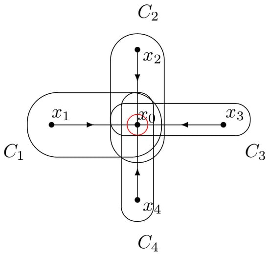
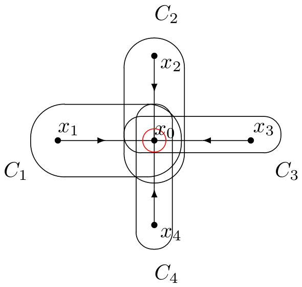
(Markov chain random field (MCRF)). Refs. [16,17] proposed MCRF model for simulating categorical spatial variables. A related spatial hidden Markov chain model is discussed in [18]. In a simplified form of MCRF ([17] [Subsection 2.2 of Section 2]), the joint distribution of (unobserved) central variable $y_{x_0}$ and (observed) $y_{x_1},\cdots ,y_{x_m}$ variables writes as

$$P(y_{x_0},y_{x_1},\cdots ,y_{x_m})=P\left(y_{x_0}\right)P\left(y_{x_1}\right|y_{x_0})P\left(y_{x_2}\right|y_{x_0})\cdots P\left(y_{x_m}\right|y_{x_0}).$$

(24)

(24) imply that $y_{x_1},y_{x_2},\cdots ,y_{x_m}$ are conditionally independent given $y_{x_0}$. Ref. [17] note that (24) does not comply with the intuitive Bayesian network with parent $x_0$ and children $x_1,\cdots ,x_m$, except for the trivial case when $y_{x_i},i=0,1,\cdots ,m$ are independent. On the other hand, (24) is a Markov cell process on cell DAG $\overrightarrow{H}\left(\mathcal{C}\right)$ consisting of $m+1$ cells $C_1=\{x_1,x_0\},\cdots ,C_m=\{x_m,x_0\},C_0=\left\{x_0\right\}$ directed as $(C_1\to C_0)\in \overrightarrow{E}\left(\mathcal{C}\right),\cdots ,(C_m\to C_0)\in \overrightarrow{E}\left(\mathcal{C}\right)$, and cell probabilities ${\pi }_i\left(y_{C_i}\right)=P(y_i,y_0),i=1,\cdots ,m$; see Figure 2. Please note that the conditional independence in (24) is exactly the NCI⁻ condition (Assumption 6 below) for the central cell $C_0$ with $C_0^{-}=C_0,j=1.$

Figure 2. Cells $C_1,\cdots ,C_m,m=4$ in Example 7. The central cell $C_0$ is shown in red.

Definition 5.

Let $\overrightarrow{H}\left(\mathcal{C}\right)=(V\left(\mathcal{C}\right),\overrightarrow{E}\left(\mathcal{C}\right))$ be a cell DAG satisfying Assumptions 1, 2, and 3. A Markov cell process $P_X$ in (21) will be called DAG reversible if

$$P_X\left(y_X\right)={\widehat{P}}_X\left(y_X\right),$$

where $P_X,{\widehat{P}}_X$ are defined in (21), (22), respectively.

Definition 6.

Let $\overrightarrow{H}\left(\mathcal{C}\right)=(V\left(\mathcal{C}\right),\overrightarrow{E}\left(\mathcal{C}\right))$ be a cell DAG satisfying Assumptions 1 and 3 and $\overrightarrow{H}\left({\mathcal{C}}^{\prime }\right)\in \mathcal{S}\left(\overrightarrow{H}\left(\mathcal{C}\right)\right)$ be a cell subDAG in (17) corresponding to a subset $V\left({\mathcal{C}}^{\prime }\right)=V^{\prime }\subset V\left(\mathcal{C}\right)=V$; $K^{\prime }:=\{i\in K:C_i\in V^{\prime }\},X^{\prime }:={\bigcup }_{i\in K^{\prime }}{C}_i$. Let $P_X,P_{X^{\prime }}$ be Markov cell processes on $\overrightarrow{H}\left(\mathcal{C}\right),\overrightarrow{H}\left({\mathcal{C}}^{\prime }\right)$, with cell distributions $\{{\pi }_i,i\in K\},\{{\pi }_i^{\prime }:={\pi }_i,i\in K^{\prime }\}$. We say that $P_X$ is consistent with regard to $\overrightarrow{H}\left({\mathcal{C}}^{\prime }\right)$ if

$$P_X\left(y_{X^{\prime }}\right)=P_{X^{\prime }}\left(y_{X^{\prime }}\right),$$

(25)

in other words, if the restriction of $P_X$ on $X^{\prime }\subset X$ coincides with $P_{X^{\prime }}$.

Proposition 3.

Let $P_X$ be a DAG reversible Markov cell process on a cell DAG $\overrightarrow{H}\left(\mathcal{C}\right)=(V\left(\mathcal{C}\right),\overrightarrow{E}\left(\mathcal{C}\right))$ be a cell DAG satisfying Assumptions 1, 2 and 3, and $\overrightarrow{H}\left({\mathcal{C}}^{\prime }\right)\in {\mathcal{S}}_{CDA}\left(\overrightarrow{H}\left(\mathcal{C}\right)\right)$ be a cell subDAG obtained from $\overrightarrow{H}\left(\mathcal{C}\right)$ by CDA (see Definition 2). Let $P_X,P_{X^{\prime }}$ be the corresponding Markov cell processes on $\overrightarrow{H}\left(\mathcal{C}\right),\overrightarrow{H}\left({\mathcal{C}}^{\prime }\right).$ Then $P_X$ is consistent with regard to $\overrightarrow{H}\left({\mathcal{C}}^{\prime }\right)$.

Proof. 

It suffices to show consistency for a one-step CDA which removes a single cell (a sink or a source) from $V\left(\mathcal{C}\right)$. Moreover, it suffices to consider the case of a top CDA $\overrightarrow{H}\left(\mathcal{C}\right){\to }_{+}\overrightarrow{H}\left({\mathcal{C}}^{\prime }\right)\in {\mathcal{S}}_{CDA}^{+}\left(\overrightarrow{H}\left(\mathcal{C}\right)\right)$ since the case of a bottom CDA follows by DAG reversibility. Let $C_k$ be a sink cell, $C_k^{+}=\varnothing$, $V\left(\mathcal{C}\right)=\{C_1,\cdots ,C_k\},V\left({\mathcal{C}}^{\prime }\right)=\{C_1,\cdots ,C_{k-1})$ as in the proof of Proposition 2. The proof of (25) for the above $\overrightarrow{H}\left({\mathcal{C}}^{\prime }\right)$ follows from (23), by noting that the l.h.s. of (23) coincides with $P_X\left(y_{X^{\prime }}\right)$. □

Remark 2.

In the case of chain DAG $X=\{1,\cdots ,n,n+1\},C_i=\{i,i+1\},(C_i\to C_j)\in \overrightarrow{E}\left(\mathcal{C}\right)⟺j=i+1,i=1,\cdots ,n$ we have that $C_1^{-}=\varnothing ,C_i^{-}=\left\{i\right\},{\tilde{C}}_i^{+}=\{i+1\},i=2,\cdots ,n$ and the Markov cell process in (21)

$$\begin{array}{ccc}\hfill P_X\left(y_X\right)& =& {\pi }_1\left(y_1\right){\pi }_1\left(y_2\right|y_1){\pi }_2\left(y_3\right|y_2)\cdots {\pi }_n\left(y_{n+1}\right|y_n)\hfill \end{array}$$

(26)

is a Markov chain with initial distribution ${\pi }_1\left(y_1\right)$ and transition probabilities ${\pi }_i\left(y_{i+1}\right|y_i).$ If the joint distributions ${\pi }_i(y_i,y_{i+1})$ are compatible in the sense that

$${\pi }_{i-1}\left(y_i\right)={\pi }_i\left(y_i\right),i=2,\cdots ,n$$

(27)

(see Assumption 5 below), the r.h.s. of (26) can be rewritten as a backward Markov chain:

$$\begin{array}{c}\hfill P_X\left(y_X\right)={\pi }_n\left(y_{n+1}\right){\pi }_n\left(y_n\right|y_{n+1}){\pi }_{n-1}\left(y_{n-1}\right|y_n)\cdots {\pi }_1\left(y_1\right|y_2)={\widehat{P}}_X\left(y_X\right),\end{array}$$

hence the Markov chain $P_X$ in (26) is DAG reversible under (27); moreover, if ${\pi }_i=\pi ,i=1,\cdots ,n$ do not depend on i, (26) is stationary with stationary distribution $\pi \left(y\right)={\sum }_{\tilde{y}}\pi (y,\tilde{y})$.

Recall that a stationary Markov chain with stationary distribution $\tilde{\pi }\left(y\right)$ and transition probabilities $\pi \left(y\right|x)=\pi (x,y)/\pi (x)$ is called reversible if

$$\tilde{\pi }\left(x\right)\pi \left(y\right|x)=\tilde{\pi }\left(y\right)\pi \left(x\right|y)(\forall x,y).$$

(28)

Equation (28) with $\tilde{\pi }\left(x\right)=\pi \left(x\right)={\sum }_y\pi (x,y)$ leads to the symmetry $\pi (x,y)=\pi (y,x)$ of the bivariate distribution, which is much stronger than the coincidence of marginals: ${\sum }_y\pi (x,y)={\sum }_y\pi (y,x)$. We conclude that DAG reversibility of a Markov chain in (26) with the same bivariate ${\pi }_i\equiv \pi$ does not imply its reversibility in the sense of (28).

4. NCI Condition and Factorization Lemma

Let $E=\left\{e\right\}$ be a finite set and $P\left(y_E\right)=P(y_e,e\in E)$ be a probability distribution on configurations $y_E=(y_e,e\in E)$. For any subset $E^{\prime }\subset E$, let

$$P\left(y_{E^{\prime }}\right)=P(y_e,e\in E^{\prime })$$

denote the restriction or marginal of $P\left(y_E\right)$ to $y_{E^{\prime }}=(y_e,e\in E^{\prime }),$ with the convention that $P\left(y_{E^{\prime }}\right):=1$ when $E^{\prime }$ is empty.

Let $E_r\subset E,r\in L:=\{1,\cdots ,\mathcal{l}\}$ be a given collection of nonempty and possibly intersecting subsets of E whose union is ${\bigcup }_{r\in L}{E}_r=E.$ With each subset $E_r$, we can associate the marginal $P\left(y_{E_r}\right)$ of $P\left(y_E\right).$ The central question of this section is when and how a distribution $P\left(y_E\right)$ can be expressed through its marginals $P\left(y_{E_r}\right),r\in L$?

The above question is obvious if $E_r,r\in L$ are disjoint and $y_{E_r},r\in L$ are independent since these conditions imply $P\left(y_E\right)={\prod }_{r\in L}P\left(y_{E_r}\right).$ However, the last expression is not true when the sets $E_r,r\in L$ intersect.

Before turning to the general case we start with some simple examples when the above question can be answered without introducing complex notation.

Example 8.

Let $P\left(y\right)={\prod }_{e\in E}P\left(y_e\right)$ be a product distribution and $E_r\subset E,r\in L$ be arbitrary. For any $S\subset L$ and the intersection $E\left(S\right)={\bigcap }_{r\in S}{E}_r$, we see that the marginal $P\left(y_{E\left(S\right)}\right)={\prod }_{e\in \cap E\left(S\right)}P\left(y_e\right)$ writes as product over $j=1,\cdots ,r$ of marginals on sets belonging to exactly j sets $E_r,r\in L.$ It is easy to check that a product distribution $P=P_E$ writes as in (3). Obviously, a product distribution satisfies the NCI condition defined in Assumption 4 below.

Example 9.

Consider the next simple case of two intersecting sets: $E_1,E_2(L=\{1,2\}),E=E_1\cup E_2,E_1\cap E_2\ne \varnothing .$ Then, $P\left(y_{E_1}\right)P\left(y_{E_2}\right)$ is not a probability distribution since ${\sum }_{y_E}P\left(y_{E_1}\right)P\left(y_{E_2}\right)={\sum }_{y_{E_1\cap E_2}}{P}^2\left(y_{E_1\cap E_2}\right)\ne 1$ except for the trivial case when $P\left(y_{E_1\cap E_2}\right)$ is concentrated at a single point. The ‘normalized’ product $P^{\prime }\left(y_E\right):=P\left(y_{E_1}\right)P\left(y_{E_2}\right)/P\left(y_{E_1\cap E_2}\right)$ is a probability but $P^{\prime }\left(y_E\right)\ne P\left(y_E\right)$ unless $y_{E_2\setminus E_1}$ are conditionally independent given $y_{E_1\cap E_2}.$ , viz.,

$$P(y_{E_1\setminus E_2},y_{E_2\setminus E_1}|y_{E_1\cap E_2})=P\left(y_{E_1\setminus E_2}\right|y_{E_1\cap E_2})P\left(y_{E_2\setminus E_1}\right|y_{E_1\cap E_2}).$$

(29)

Indeed, from (29) and the definition of conditional probability, we get

$$\begin{array}{ccc}\hfill P\left(y_E\right)& =& P(y_{E_1\setminus E_2},y_{E_2\setminus E_1},y_{E_1\cap E_2})=P(y_{E_1\setminus E_2},y_{E_2\setminus E_1}|y_{E_1\cap E_2})P\left(y_{E_1\cap E_2}\right)\hfill \\ & =& {\displaystyle \frac{P\left(y_{E_1\setminus E_2}\right|y_{E_1\cap E_2})P\left(y_{E_1\cap E_2}\right)P\left(y_{E_2\setminus E_1}\right|y_{E_1\cap E_2})P\left(y_{E_1\cap E_2}\right)}{P\left(y_{E_1\cap E_2}\right)}}\hfill \\ & =& {\displaystyle \frac{P\left(y_{E_1}\right)P\left(y_{E_2}\right)}{P\left(y_{E_1\cap E_2}\right)}}=P^{\prime }\left(y_E\right).\hfill \end{array}$$

(30)

Equation (29) is the NCI condition for $\left|L\right|=\mathcal{l}=2$, resulting in the representation (30) of $P\left(y_E\right)$ through three marginals $P\left(y_{E_1}\right),P\left(y_{E_2}\right)$, and $P\left(y_{E_1\cap E_2}\right)$.

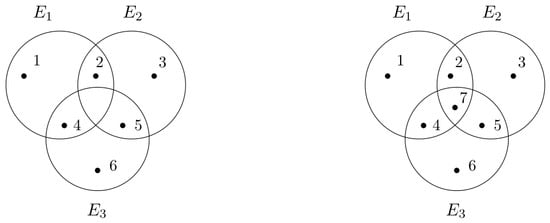
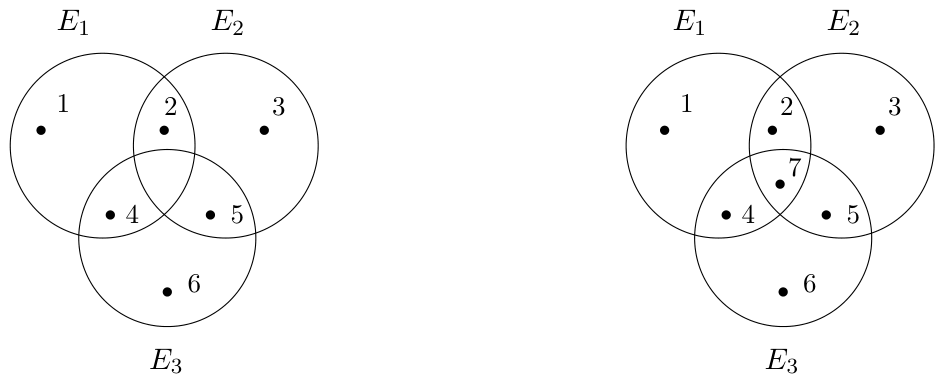
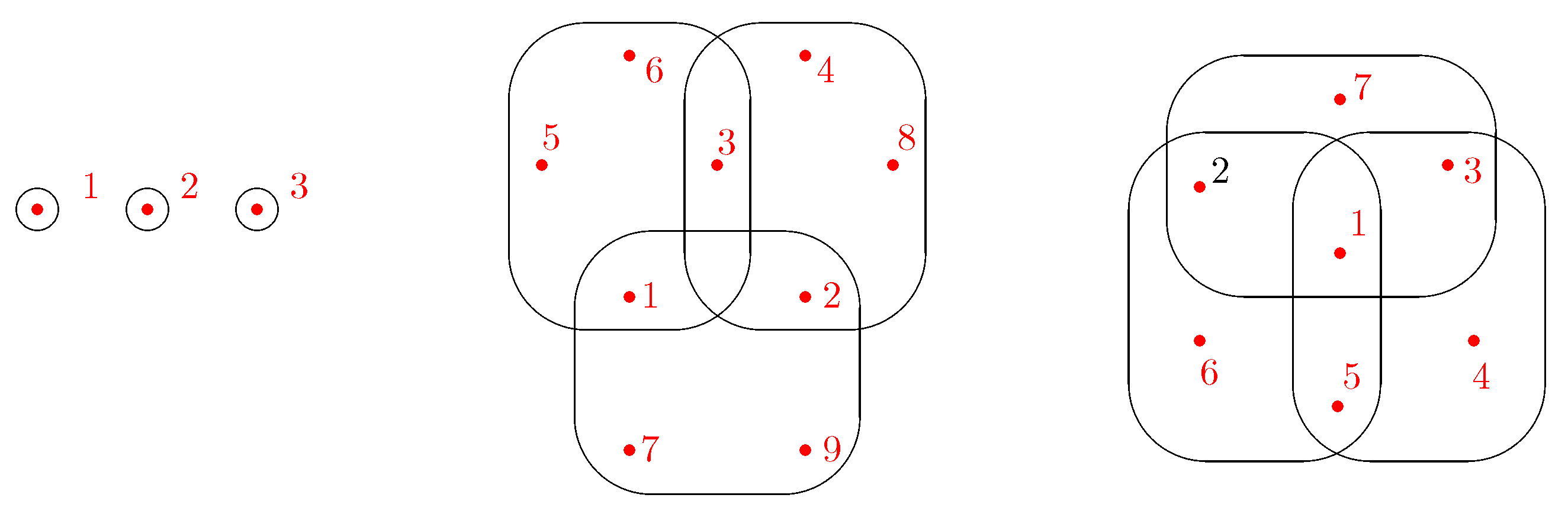
For $\left|L\right|\ge 3$, the NCI condition is more involved and includes several ‘nested’ conditional independence equations. The two examples shown in Figure 3 deal with 3 sets $E_r,r\in L=\{1,2,3\}$ and correspond to cases ${\mathrm{E}}_1\cap E_2\cap E_3=\varnothing$ (Figure 3, left) and ${\mathrm{E}}_1\cap E_2\cap E_3\ne \varnothing$ (Figure 3, right). Formulas (31) and (32) for $P\left(y_E\right)$ in these examples agree with (3) and (36) of (factorization) Lemma 1. We also note that Example 11 appears in the past diagram of Model V, Section 6.

Figure 3. Sets $E_1,E_2,E_3$ in Example 10 (left) and Example 11 (right).

Example 10

(Figure 3, left). Let $E=\{1,2,3,4,5,6\},E_1=\{1,2,4\},E_2=\{2,3,5\},E_3=\{4,5,6\}.$ Then

$$\begin{array}{ccc}\hfill & & E(1,2)=E_1\cap E_2=\left\{2\right\},E(1,3)=E_1\cap E_3=\left\{4\right\},E(2,3)=E_2\cap E_3=\left\{5\right\}.\hfill \end{array}$$

The NCI conditions (34) and (35) in this example translate to (i)–(ii):

(i) 

marginals $y_1,y_3,y_6$ are conditionally independent given $(y_2,y_4,y_5)$:

$$P(y_1,y_3,y_6|y_2,y_4,y_5)=P\left(y_1\right|y_2,y_4,y_5)P\left(y_3\right|y_2,y_4,y_6)P\left(y_6\right|y_2,y_4,y_5);$$

moreover, the above conditional distributions depend only those $y_i,i=2,4,5$ whose indices fall into respective sets $E_i,i=1,2,3$:

$$P\left(y_1\right|y_2,y_4,y_5)=P\left(y_1\right|y_2,y_4),P\left(y_3\right|y_2,y_4,y_5)=P\left(y_3\right|y_2,y_5),P\left(y_6\right|y_2,y_4,y_5)=P\left(y_6\right|y_4,y_5);$$

(ii) 

$y_2,y_4,y_5$ are independent: $P(y_2,y_4,y_5)=P\left(y_2\right)P\left(y_4\right)P\left(y_5\right).$

Similarly to (30), one can directly derive from (i)–(ii) a representation of $P\left(y_E\right)$ through its marginals (factorization formula):

$$\begin{array}{ccc}\hfill P\left(y_E\right)& =& {\displaystyle \frac{P\left(y_{E_1}\right)P\left(y_{E_2}\right)P\left(y_{E_3}\right)}{P\left(y_{E_1\cap E_2}\right)P\left(y_{E_1\cap E_3}\right)P\left(y_{E_2\cap E_3}\right)}}.\hfill \end{array}$$

(31)

Example 11

(Figure 3, right). Let $E=\{1,2,3,4,5,6,7\},E_1=\{1,2,4,7\},E_2=\{2,3,5,7\},$$E_3=\{4,5,6,7\}.$ We have

$$\begin{array}{ccc}& & E(1,2)=\{2,7\},E(1,3)=\{4,7\},E(2,3)=\{5,7\},E(1,2,3)=\left\{7\right\}.\hfill \end{array}$$

The NCI conditions (34) and (35) in this example translate to (j)–(jj) below:

(j) 

marginals $y_1,y_3,y_6$ are conditionally independent given $(y_2,y_4,y_5,y_7)$:

$$P(y_1,y_3,y_6|y_2,y_4,y_5,y_7)=P\left(y_1\right|y_2,y_4,y_5,y_7)P\left(y_3\right|y_2,y_4,y_6,y_7)P\left(y_6\right|y_2,y_4,y_5,y_7).$$

Moreover, $P\left(y_1\right|y_2,y_4,y_5,y_7)=P\left(y_1\right|y_2,y_4,y_7),P\left(y_3\right|y_2,y_4,y_5,y_7)=P\left(y_3\right|y_2,y_5,y_7),$ $P\left(y_6\right|y_2,y_4,y_5,y_7)=P\left(y_6\right|y_4,y_5,y_7);$

(jj) 

$y_2,y_4,y_5$ are conditionally independent given $y_7$: $P(y_2,y_4,y_5|y_7)=P\left(y_2\right|y_7)P\left(y_4\right|y_7)$ $\times P\left(y_5\right|y_7).$

From (j)–(jj), we derive the factorization formula:

$$\begin{array}{ccc}\hfill P\left(y_E\right)& =& P(y_1,y_3,y_6|y_2,y_4,y_5,y_7)P(y_2,y_4,y_5|y_7)P\left(y_7\right)\hfill \\ & =& P\left(y_1\right|y_2,y_4,y_7)P\left(y_3\right|y_2,y_5,y_7)P\left(y_6\right|y_4,y_5,y_7)P\left(y_2\right|y_7)P\left(y_4\right|y_7)P\left(y_5\right|y_7)P\left(y_7\right)\hfill \\ & =& {\displaystyle \frac{P(y_1,y_2,y_4,y_7)P(y_2,y_3,y_5,y_7)P(y_4,y_5,y_6,y_7)P\left(y_2\right|y_7)P\left(y_4\right|y_7)P\left(y_5\right|y_7)P\left(y_7\right)}{P^2\left(y_2\right|y_7)P^4\left(y_4\right|y_7)P^2\left(y_5\right|y_7)P^3\left(y_7\right)}}\hfill \\ & =& {\displaystyle \frac{P\left(y_{E_1}\right)P\left(y_{E_2}\right)P\left(y_{E_3}\right)P\left(y_{E_1\cap E_2\cap E_3}\right)}{P\left(y_{E_1\cap E_2}\right)P\left(y_{E_1\cap E_3}\right)P\left(y_{E_2\cap E_3}\right)}}\hfill \end{array}$$

(32)

Let us turn to the formulations of NCI conditions in the general case $E_r\subset E,r\in L$. For any $S\subset L,\left|S\right|\ge 1$ let

$$E\left(S\right):=\bigcap _{r\in S}{E}_r,\mathbf{E}\left(j\right):=\bigcup _{\left|S\right|=j}E\left(S\right)$$

Thus, $E\left(S^{\prime }\right)\subset E\left(S\right)$ for $S\subset S^{\prime }$, that is, $E\left(S\right)$ monotonically decreases as S increases. Similarly, $\mathbf{E}\left(j\right)$ monotonically decreases with j. Let $j_{\max }\le \mathcal{l}$ be the maximal j when $\mathbf{E}\left(j\right)$ is nonempty: $j_{\max }=\max \{j\ge 1:\mathbf{E}\left(j\right)\ne \varnothing \}.$

For any $S\subset L$, we decompose $E\left(S\right)=E_0\left(S\right)\cup E_{>}\left(S\right)$ as

$$E_0\left(S\right)=E\left(S\right)\setminus \mathbf{E}\left(\right|S|+1),E_{>}\left(S\right)=E\left(S\right)\cap \mathbf{E}\left(\right|S|+1).$$

(33)

That is, $E_0\left(S\right)$ consists of those $e\in E\left(S\right)$ that belong to exactly $\left|S\right|$ intersections and do not belong to any intersection $E\left(S^{\prime }\right),|S^{\prime }|=|S|+1$. In particular, $E_{i,0}\equiv E_0\left(\left\{i\right\}\right)$ contains points of $E_i$ that do not belong to any other $E_j,j\ne i.$

Assumption 4.

We say that a (discrete) probability distribution $P\left(y_E\right)$ satisfies nested conditional independence (NCI) condition with respect to sets $E_1,\cdots ,E_{\mathcal{l}}$ if for any $1\le j\le j_{\max }$ random vectors $y_{E_0\left(S\right)},\left|S\right|=j$ are conditionally independent given $y_{\mathbf{E}(j+1)}$, viz.,

$$P\left(y_{E_0\left(S\right)},\left|S\right|=j|y_{\mathbf{E}(j+1)}\right)=\prod _{\left|S\right|=j}P\left(y_{E_0\left(S\right)}\right|y_{\mathbf{E}(j+1)})$$

(34)

Moreover,

$$P\left(y_{E_0\left(S\right)}\right|y_{\mathbf{E}(j+1)})=P\left(y_{E_0\left(S\right)}\right|y_{E_{>}\left(S\right)}),\left|S\right|=j=1,2,\cdots .$$

(35)

Remark 3.

For $j=j_{\max }$, (34) reduces to the independence of random vectors $y_{E_0\left(S\right)},\left|S\right|=j_{\max }.$

The following example details the NCI condition for the cell graph in Figure 6, middle (Model E of Section 6).

Example 12.

$E=\{1,2,3,4,5,6,7,8,9\},\mathcal{l}=3$, $E_1=\{2,3,4,8\},$$E_2=\{1,3,5,6\},$$E_3=\{1,2,7,9\}$. We have $j_{\max }=2,\mathbf{E}\left(2\right)=\{1,2,3\},$

$$\begin{array}{ccc}& & E(1,2)=E_1\cap E_2=\left\{3\right\},E(1,3)=E_1\cap E_3=\left\{2\right\},E(2,3)=E_2\cap E_3=\left\{1\right\},\hfill \\ & & E_{3,0}=\{7,9\},E_{2,0}=\{5,6\},E_{1,0}=\{4,8\}.\hfill \end{array}$$

The NCI conditions (34) and (35) in this example translate to (i)–(ii):

(i) 

random vectors $y_{E_{1,0}}=(y_4,y_8),y_{E_{2,0}}=(y_5,y_6),y_{E_{3.0}}=(y_7,y_9)$ are conditionally independent given $y_{\mathrm{E}\left(2\right)}=(y_1,y_2,y_3)$:

$$P(y_4,y_8,y_5,y_6,y_7,y_9|y_1,y_2,y_3)=P(y_4,y_8|y_1,y_2,y_3)P(y_5,y_6|y_1,y_2,y_3)P(y_7,y_9|y_1,y_2,y_3),$$

moreover, $P(y_4,y_8|y_1,y_2,y_3)=P(y_4,y_8|y_2,y_3),P(y_5,y_6|y_1,y_2,y_3)=P(y_5,y_6|y_1,y_3),P(y_7,y_9|y_1,y_2,y_3)=P(y_7,y_9|y_1,y_2);$

(ii) 

$y_{E_0(1,2)}=y_3,y_{E_0(1,3)}=y_2,y_{E_0(2,3)}=y_1$ are independent: $P(y_3,y_2,y_1)=P\left(y_3\right)P\left(y_2\right)P\left(y_1\right).$

Lemma 1

(Factorization lemma). Assume that $P\left(y_E\right)$ satisfies the nested conditional independence (NCI) condition with respect to $E_1,\cdots ,E_{\mathcal{l}}$ (Assumption 4). Then,

$$P\left(y_E\right)={\displaystyle \frac{{\prod }_{\left|S\right|=1}P\left(y_{E\left(S\right)}\right)}{{\prod }_{\left|S\right|=2}P\left(y_{E\left(S\right)}\right)}}\times {\displaystyle \frac{{\prod }_{\left|S\right|=3}P\left(y_{E\left(S\right)}\right)}{{\prod }_{\left|S\right|=4}P\left(y_{E\left(S\right)}\right)}}\times \cdots \times \left\{\begin{array}{cc}{\displaystyle \frac{{\prod }_{\left|S\right|=j_{\max }}P\left(y_{E\left(S\right)}\right)}{1}},\hfill & \mathit{if}{j}_{\max }\mathit{is}\mathit{odd},\hfill \\ {\displaystyle \frac{{\prod }_{\left|S\right|=j_{\max }-1}P\left(y_{E\left(S\right)}\right)}{{\prod }_{\left|S\right|=j_{\max }}P\left(y_{E\left(S\right)}\right)}},\hfill & \mathit{if}{j}_{\max }\mathit{is}\mathit{even}.\hfill \end{array}\right.$$

(36)

Proof. 

We use the induction on the number $n:=\left|E\right|$ of elements of the set E. The lemma is obviously true for $n=2,3.$ Assume that it is true for any finite set $\tilde{E}$ with $\left|\tilde{E}\right|<n.$ We need to show that it remains true for $E,\left|E\right|=n.$

To prove the induction step, assume first that $\mathbf{E}\left(1\right)\setminus \mathbf{E}\left(2\right)=:{\mathbf{E}}_0\left(1\right)$ is nonempty. In such case, we remove this set from $E=\mathbf{E}\left(1\right)$ and apply the inductive assumption to $\tilde{E}:=E\setminus {\mathbf{E}}_0\left(1\right)=\mathbf{E}\left(2\right)$ as follows. We have

$$P\left(y_E\right)=P(y_{\tilde{E}},y_{{\mathbf{E}}_0\left(1\right)})=P(y_{{\mathbf{E}}_0\left(1\right)},y_{\mathbf{E}\left(2\right)})=P\left(y_{{\mathbf{E}}_0\left(1\right)}\right|y_{\mathbf{E}\left(2\right)})P\left(y_{\tilde{E}}\right),$$

(37)

where

$$P\left(y_{{\mathbf{E}}_0\left(1\right)}\right|y_{\mathbf{E}\left(2\right)})=\prod _{\left|S\right|=1}P\left(y_{E_0\left(S\right)}\right|y_{E_{>}\left(S\right)})$$

according to NCI for $j=1$. The inductive assumption of (36) for $\tilde{E}$ is written as

$$P\left(y_{\tilde{E}}\right)={\displaystyle \frac{{\prod }_{\left|S\right|=1}P\left(y_{\tilde{E}\left(S\right)}\right)}{{\prod }_{\left|S\right|=2}P\left(y_{\tilde{E}\left(S\right)}\right)}}\times {\displaystyle \frac{{\prod }_{\left|S\right|=3}P\left(y_{\tilde{E}\left(S\right)}\right)}{{\prod }_{\left|S\right|=4}P\left(y_{\tilde{E}\left(S\right)}\right)}}\times \cdots \times \left\{\begin{array}{cc}{\displaystyle \frac{{\prod }_{\left|S\right|={\tilde{j}}_{\max }}P\left(y_{\tilde{E}\left(S\right)}\right)}{1}},\hfill & \mathrm{if}{\tilde{j}}_{\max }\mathrm{is}\mathrm{odd},\hfill \\ {\displaystyle \frac{{\prod }_{\left|S\right|={\tilde{j}}_{\max }-1}P\left(y_{\tilde{E}\left(S\right)}\right)}{{\prod }_{\left|S\right|={\tilde{j}}_{\max }}P\left(y_{\tilde{E}\left(S\right)}\right)}},\hfill & \mathrm{if}{\tilde{j}}_{\max }\mathrm{is}\mathrm{even}.\hfill \end{array}\right.$$

(38)

where

$$\tilde{E}\left(S\right)=\left\{\begin{array}{cc}{E}_{>}\left(S\right),\hfill & \left|S\right|=1,\hfill \\ E\left(S\right),\hfill & \left|S\right|\ge 2,\hfill \end{array}\right.$$

(39)

${\tilde{j}}_{\max }=j_{\max }.$ Relations (37)–(39) together with $P\left(y_{E_0\left(S\right)}\right|y_{E_{>}\left(S\right)})P\left(y_{E_{>}\left(S\right)}\right)=P\left(y_{E\left(S\right)}\right)$ lead to (38), thus proving the induction step in the case when ${\mathbf{E}}_0\left(1\right)$ is not empty.

Assume now that $E=\mathbf{E}\left(2\right)$, i.e., ${\mathbf{E}}_0\left(1\right)$ is empty but $E\setminus \mathbf{E}\left(3\right)=\mathbf{E}\left(2\right)\setminus \mathbf{E}\left(3\right)=:{\mathbf{E}}_0\left(2\right)$ is nonempty. Then, we remove ${\mathbf{E}}_0\left(2\right)$ from E and define $\tilde{E}:=E\setminus {\mathbf{E}}_0\left(2\right)$ similarly as in the previous case, with $\left|\tilde{E}\right|<\left|E\right|.$ We have $P\left(y_E\right)=P\left(y_{{\mathbf{E}}_0\left(2\right)}\right|y_{\mathbf{E}\left(3\right)})P\left(y_{\tilde{E}}\right)$ as in (37), where $P\left(y_{{\mathbf{E}}_0\left(2\right)}\right|y_{\mathbf{E}\left(3\right)})={\prod }_{\left|S\right|=2}P\left(y_{E_0\left(S\right)}\right|y_{E_{>}\left(S\right)})$ according to NCI for $j=2$. The application of the inductive assumption to the above $\tilde{E}$ continues as in the previous case. The proof in the general case proceeds as above and is omitted. □

Remark 4.

In the following, we shall write the right-hand sides of (36), (37) and other similar expressions as ${\displaystyle \frac{{\prod }_{\left|S\right|=1}\cdots }{{\prod }_{\left|S\right|=2}\cdots }}\times {\displaystyle \frac{{\prod }_{\left|S\right|=3}\cdots }{{\prod }_{\left|S\right|=4}\cdots }}\times \cdots$, omitting the last term for brevity.

5. Consistent and DAG Reversible Cell Processes

Let us return to a Markov cell process $P_X\left(y_X\right)$ on a cell DAG $\overrightarrow{H}\left(\mathcal{C}\right)=(V\left(\mathcal{C}\right),\overrightarrow{E}\left(\mathcal{C}\right))$, defined in Definition 4 for a given family of cells $C_i,i\in K$ and cell distributions ${\pi }_i,i\in K.$ The distribution $P_X$ in (21) is written as a product of conditional probabilities ${\pi }_i(y_{{\tilde{C}}_i^{+}}|y_{C_i^{-}})$ involving cell pasts $C_i^{-}$. A Markov cell process ${\widehat{P}}_X$ on the reversed DAG $\begin{array}{c}\overleftarrow{H}\end{array}\left(\mathcal{C}\right)=(V\left(\mathcal{C}\right),\begin{array}{c}\overleftarrow{E}\end{array}\left(\mathcal{C}\right))$ is defined analogously in (22) as a product of conditional probabilities ${\pi }_i(y_{{\tilde{C}}_i^{+}}|y_{C_i^{+}})$. We show in Theorem 1 that, under additional conditions on marginals ${\pi }_i(y_{C_i^{\pm }})$ and $\overrightarrow{H}\left(\mathcal{C}\right)$, the two processes $P_X$ and ${\widehat{P}}_X$ coincide—$P_X\left(y_X\right)={\widehat{P}}_X\left(y_X\right)$—and satisfy the consistency property with regard to cell subDAGs obtained by CDA (cell dismantling algorithm). The crucial point for establishing the coincidence $P_X={\widehat{P}}_X$ (termed DAG reversibility) is the factorization formula in (50) similar to (36), which allows us to write $P_X$ as a product of ratios of cell distributions on intersection sets

$$C\left(S\right):=\bigcap _{i\in S}{C}_i,S\subset K.$$

(40)

Let us turn to rigorous formulations of Assumptions 5–7 of Theorem 1.

Assumption 5

(Compatibility). For any $i,j\in K$

$${\pi }_i\left(y_{C_i\cap C_j}\right)={\pi }_j\left(y_{C_i\cap C_j}\right).$$

(41)

Assumption 5 allows us to define cell distribution ${\pi }_S\left(y_{C_S}\right)$ for intersection sets $C_S$ in (40) as

$${\pi }_S\left(y_{C\left(S\right)}\right):={\pi }_i\left(y_{C\left(S\right)}\right),i\in S$$

(42)

since the r.h.s. of (40) does not depend on $i\in S$ n view of (41).

Next, we introduce NCI^± conditions for future/past cell parts. In the general case, these conditions involve additional and somewhat complex notation; the reader is advised to Examples 13 and 14, and Figure 4, Figure 5 and Figure 6, for illustration.

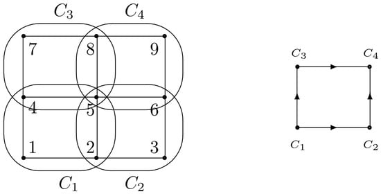
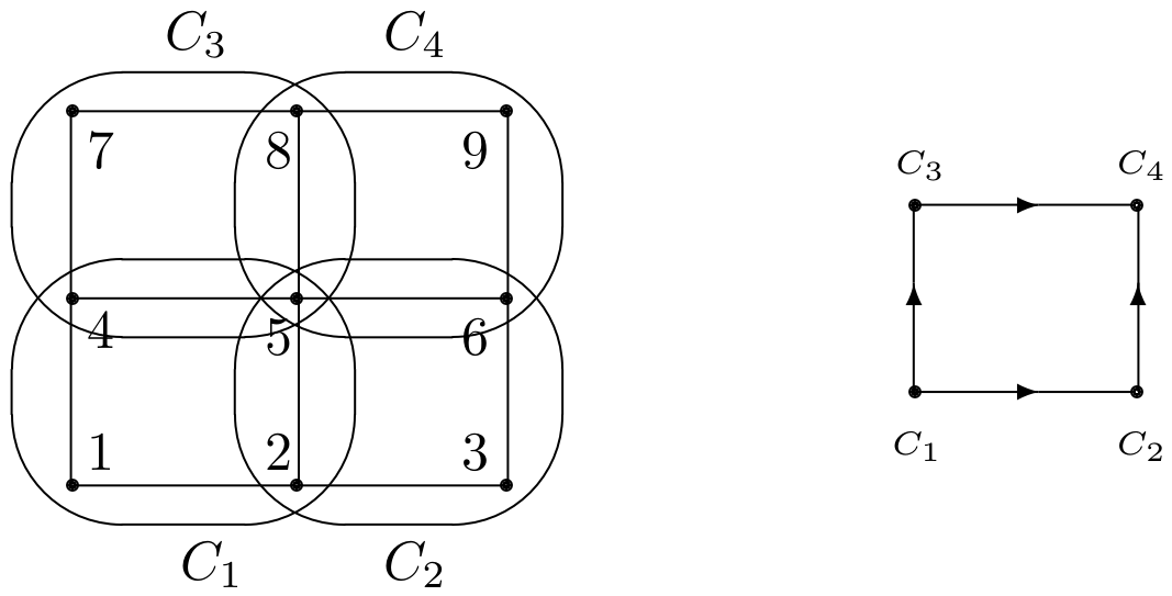
Figure 4. The Pickard model on $2\times 2$ rectangle V. Left: cells $C_1,C_2,C_3,C_4$, right: cell DAG $\overrightarrow{H}\left(\mathcal{C}\right)$.

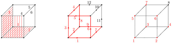
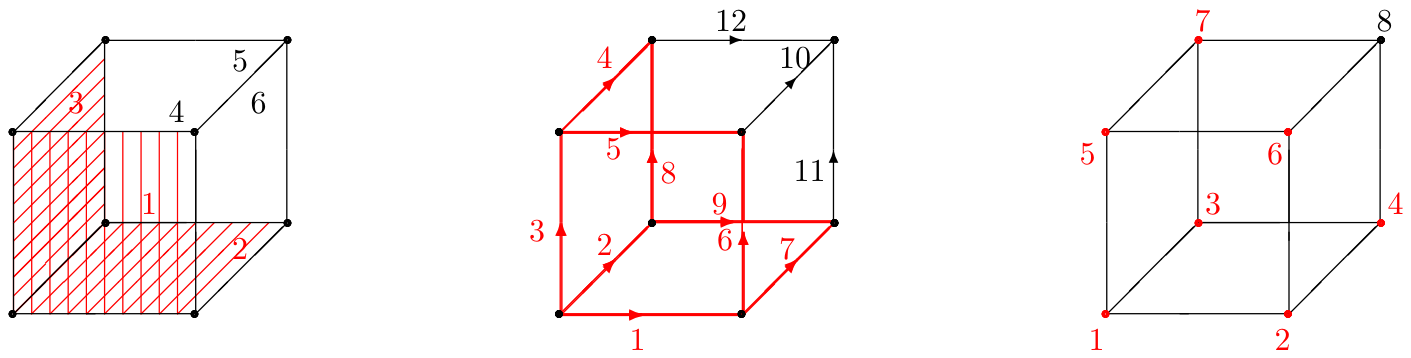
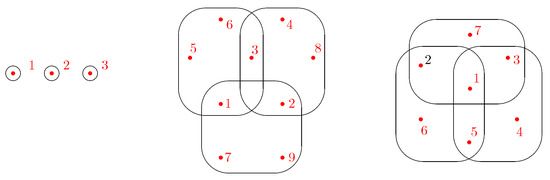
Figure 5. Generic cell $C_{\mathit{x}}$, cell past $C_{\mathit{x}}^{-}$ in red. From left to right: Model F; Model E; Model V.

Figure 6. Past diagrams for cells in Figure 5. From left to right: Model F; Model E; Model V. The colors in Figure 6 correspond to the colors in Figure 5.

Recall the cell decomposition in (6): for any $i\in K$, we have $C_i=C_i^{-}\cup {\tilde{C}}_i^{-}=C_i^{+}\cup {\tilde{C}}_i^{+}$, where

$$C_i^{-}:=\bigcup _{(C_r\to C_i)\in \overrightarrow{E}\left(\mathcal{C}\right)}{C}_r\cap C_i(\mathrm{past}\mathrm{of}{C}_i),C_i^{+}:=\bigcup _{(C_i\to C_r)\in \overrightarrow{E}\left(\mathcal{C}\right)}{C}_r\cap C_i(\mathrm{future}\mathrm{of}{C}_i)$$

(43)

and where ${\tilde{C}}_i^{\pm }:=C_i\setminus C_i^{\pm }$. In other words, $C_i^{-}$ (and $C_i^{+}$) is the part of $C_i$ covered by all parent (respectively, children) cells of $C_i$. The sets of such parent/children cells are denoted

$$L_i^{-}:=\{r\in K:(C_r\to C_i)\in \overrightarrow{E}\left(\mathcal{C}\right)\},L_i^{+}:=\{r\in K:(C_i\to C_r)\in \overrightarrow{E}\left(\mathcal{C}\right)\}.$$

Let

$$C_{i,r}^{\pm }:=C_i\cap C_r,r\in L_i^{\pm }.$$

(44)

be part of $C_i$ covered by the child (parent) $C_r$. We will also need to introduce the parts of $C_i$ covered by several children (parents). Consequently, for any $S\subset L_i^{\pm },\left|S\right|\ge 1$, denote

$$C_i^{\pm }\left(S\right):=\bigcap _{r\in S}{C}_{i,r}^{\pm },{\mathbf{C}}_i^{\pm }\left(j\right):=\bigcup _{\left|S\right|=j}{C}_i^{\pm }\left(S\right)$$

(45)

the intersection sets and their unions for collections $\{C_{i,r}^{\pm };r\in L_i^{\pm }\}$ of subsets of the ‘future’/‘past’ parts $C_i^{\pm }$ of a cell $C_i$. The sets $C_i^{\pm }\left(S\right)$ are further decomposed as in (33), viz.,

$$C_{i,0}^{\pm }\left(S\right):=C_i^{\pm }\left(S\right)\setminus {\mathbf{C}}_i^{\pm }\left(\right|S|+1),C_{i,>}^{\pm }\left(S\right)=C_i^{\pm }\left(S\right)\cap {\mathbf{C}}_i^{\pm }\left(\right|S|+1).$$

(46)

The sets $C_i^{\pm }$ with their subsets $C_{i,r}^{\pm },r\in L_i^{\pm }$ form future/past diagram of cell $C_i$, which can be visualized as in Figure 6 and may help better understand definitions (45), (46).

Assumption 6

(The NCI^± condition for future/past cell distributions). For any $i\in K$, the cell distribution ${\pi }_i$ satisfies the NCI^± conditions with regard to collections $\{C_{i,r}^{\pm };r\in L_i^{\pm }\}$. More explicitly, for any $j\ge 1$ random vectors $y_{C_{i,0}^{\pm }\left(S\right)},\left|S\right|=j$ are conditionally independent given $y_{{\mathbf{C}}_i^{\pm }(j+1)}$, viz.,

$${\pi }_i\left(y_{C_{i,0}^{\pm }\left(S\right)},\left|S\right|=j|y_{{\mathbf{C}}_i^{\pm }(j+1)}\right)=\prod _{\left|S\right|=j}{\pi }_i\left(y_{C_{i,0}^{\pm }\left(S\right)}\right|y_{{\mathbf{C}}_i^{\pm }(j+1)});$$

(47)

moreover,

$${\pi }_i\left(y_{C_{i,0}^{\pm }\left(S\right)}\right|y_{{\mathbf{C}}_i^{\pm }(j+1)})={\pi }_i\left(y_{C_{i,0}^{\pm }\left(S\right)}\right|y_{C_{i,>}^{\pm }\left(S\right)}),\forall \left|S\right|=j.$$

(48)

In Theorem 1, (50) products ${\mathrm{\Pi }}_{\left|S\right|=j}$ are taken over (directed) cell clique sets $\{C_i,i\in S\}$ identified with subsets $S\subset K$ and defined as follows.

Definition 7.

A set $S\subset K,\left|S\right|\ge 2$ is said to be a cell in-clique if $(C_j\to C_{i_{+}})\in \overrightarrow{E}\left(\mathcal{C}\right)$ for some $i_{+}\in S$ and any $j\in S\setminus \left\{i_{+}\right\}$. Analogously, a set $S\subset K,\left|S\right|\ge 2$ is said a cell out-clique if $(C_j\to C_{i_{-}})\in \begin{array}{c}\overleftarrow{E}\end{array}\left(\mathcal{C}\right)$ for some $i_{-}\in S$ and any $j\in S\setminus \left\{i_{-}\right\}$. By definition, $S=\left\{i\right\},\left|S\right|=1$ is a trivial in/out-cell clique.

Assumption 7.

There exists a 1-1 correspondence $S\leftrightarrow S^{\prime }$ between cell in-cliques S and cell out-cliques $S^{\prime }$ such that $\left|S\right|=|S^{\prime }|$ and ${\pi }_S\left(y_{C\left(S\right)}\right)={\pi }_{S^{\prime }}\left(y_{C\left(S^{\prime }\right)}\right)$.

We remark that Assumption 7 is satisfied in the case of edge clique cells (Example 1), since any cell in-clique S can be identified with edge $e=(v\to v^{\prime })\in \overrightarrow{E}$ in (10) which coincides with the cell out-clique (a cell in-clique $e^{\prime }=(v^{\prime }\to v)$ in the reversed cell DAG) and ${\pi }_v\left(y_e\right)={\pi }_{v^{\prime }}\left(e^{\prime }\right)$ holds by compatibility of ${\pi }_v$’s. The following proposition extends this observation to more general graphs.

Proposition 4.

Let any two connected cells be directed, that is, $C_i\cap C_j\ne \varnothing$ implies $(C_i\to C_j)\in \overrightarrow{E}\left(\mathcal{C}\right)\cup \begin{array}{c}\overleftarrow{E}\end{array}\left(\mathcal{C}\right),i,j\in K,i\ne j.$ Then, the sets of cell in-cliques and cell out-cliques coincide and Assumption 7 holds.

Proof. 

Let any two connected cells be directed. Let us show that S is a cell in-clique if and only if

$$C\left(S\right):=\bigcap _{i\in S}{C}_i\ne \varnothing .$$

(49)

Indeed, let S be a cell in-clique, then (49) holds and $C\left(S\right)=C_{i_{+}}^{-}$. Conversely, let $S\subset K$ and $C\left(S\right)\ne \varnothing .$ Then, $V_S\left(\mathcal{C}\right):=\{C_i,i\in S\}$ form is the set of vertices of the subgraph ${\overrightarrow{H}}_S\left(\mathcal{C}\right)=(V_S\left(\mathcal{C}\right),{\overrightarrow{E}}_S\left(\mathcal{C}\right))$ with ${\overrightarrow{E}}_S\left(\mathcal{C}\right)=\{(C_i\to C_j)\in \overrightarrow{E}\left(\mathcal{C}\right)),i,j\in S\}$. The cell graph ${\overrightarrow{H}}_S\left(\mathcal{C}\right)$ is acyclic and a complete graph: any vertices $C_i,C_j,i,j\in S$ are connected: $C_i\cap C_j\ne \varnothing$ since $C\left(S\right)\ne \varnothing .$ Therefore, ${\overrightarrow{H}}_S\left(\mathcal{C}\right)$ has a unique sink $C_{i_{+}},i_{+}\in S$ with the property that $(C_j\to C_i)\in {\overrightarrow{E}}_S\left(\mathcal{C}\right)),j\in S\setminus \left\{i_{+}\right\}$. Analogously, S is an cell out-clique if and only if (49) holds. Proposition 4 is proved. □

Theorem 1.

Let $P_X\left(y_X\right)$ be a Markov cell process on a cell DAG $\overrightarrow{H}\left(\mathcal{C}\right)=(V\left(\mathcal{C}\right),\overrightarrow{E}\left(\mathcal{C}\right))$ satisfying Assumptions 2, 3, 5, 6, and 7. Then, $P_X$ is DAG reversible and

$$\begin{array}{ccc}\hfill P_X\left(y_X\right)& =& {\displaystyle \frac{{\prod }_{\left|S\right|=1}^{\mathrm{in}}{\pi }_S\left(y_{C\left(S\right)}\right)}{{\prod }_{\left|S\right|=2}^{\mathrm{in}}{\pi }_S\left(y_{C\left(S\right)}\right)}}\times {\displaystyle \frac{{\prod }_{\left|S\right|=3}^{\mathrm{in}}{\pi }_S\left(y_{C\left(S\right)}\right)}{{\prod }_{\left|S\right|=4}^{\mathrm{in}}{\pi }_S\left(y_{C\left(S\right)}\right)}}\times \cdots ,\hfill \end{array}$$

(50)

$$\begin{array}{ccc}\hfill {\widehat{P}}_X\left(y_X\right)& =& {\displaystyle \frac{{\prod }_{\left|S\right|=1}^{\mathrm{out}}{\pi }_S\left(y_{C\left(S\right)}\right)}{{\prod }_{\left|S\right|=2}^{\mathrm{out}}{\pi }_S\left(y_{C\left(S\right)}\right)}}\times {\displaystyle \frac{{\prod }_{\left|S\right|=3}^{\mathrm{out}}{\pi }_S\left(y_{C\left(S\right)}\right)}{{\prod }_{\left|S\right|=4}^{\mathrm{out}}{\pi }_S\left(y_{C\left(S\right)}\right)}}\times \cdots ,\hfill \end{array}$$

(51)

where the product ${\prod }_{\left|S\right|=j}^{\mathrm{in}}$ (and ${\prod }_{\left|S\right|=j}^{\mathrm{out}}$) is taken over all cell in-cliques S (over all cell out-cliques S, respectively) of cardinality $\left|S\right|=j.$ As a consequence, $P_X$ is consistent with regard to any cell sub-DAG $\overrightarrow{H}\left({\mathcal{C}}^{\prime }\right)$ obtained from $\overrightarrow{H}\left(\mathcal{C}\right)$ by CDA.

Proof. 

Let us prove (50). From the definition (21),

$$\begin{array}{ccc}\hfill P_X\left(y_X\right)& =& \prod _{i\in K}{\pi }_i\left(y_{C_i}\right)/\prod _{i\in K}{\pi }_i\left(y_{C_i^{-}}\right),\hfill \end{array}$$

where ${\prod }_{i\in K}{\pi }_i\left(y_{C_i}\right)={\prod }_{\left|S\right|=1}^{\mathrm{in}}{\pi }_S\left(y_{C\left(S\right)}\right)={\prod }_{\left|S\right|=1}^{\mathrm{out}}{\pi }_S\left(y_{C\left(S\right)}\right)$. Hence, (50) follows from

$$\begin{array}{ccc}\hfill \prod _{i\in K}{\pi }_i\left(y_{C_i^{-}}\right)& =& {\displaystyle \frac{{\prod }_{\left|S\right|=2}^{\mathrm{in}}{\pi }_S\left(y_{C\left(S\right)}\right)}{{\prod }_{\left|S\right|=3}^{\mathrm{in}}{\pi }_S\left(y_{C\left(S\right)}\right)}}\times {\displaystyle \frac{{\prod }_{\left|S\right|=4}^{\mathrm{in}}{\pi }_S\left(y_{C\left(S\right)}\right)}{{\prod }_{\left|S\right|=5}^{\mathrm{in}}{\pi }_S\left(y_{C\left(S\right)}\right)}}\times \cdots .\hfill \end{array}$$

(52)

From Lemma 1, we can express each ${\pi }_i\left(y_{C_i^{-}}\right)$ on the l.h.s. of (52) as a product of ratios similar to the r.h.s. of (52), as follows. Namely, we apply Lemma 1 to $E=C_i^{-}$ and its subsets $E_{r,i}=C_{r,i}^{-},r\in L_i^{-}$ in (44) formed by intersections $E_{r,i}:=C_i\cap C_r$ with ‘past’ cells $C_r\to C_i$. Then,

$$\begin{array}{ccc}\hfill {\pi }_i\left(y_{C_i^{-}}\right)& =& {\displaystyle \frac{{\prod }_{|S_i|=1}{\pi }_i\left(y_{C_i^{-}\left(S_i\right)}\right)}{{\prod }_{|S_i|=2}{\pi }_i\left(y_{C_i^{-}\left(S_i\right)}\right)}}\times {\displaystyle \frac{{\prod }_{|S_i|=3}{\pi }_i\left(y_{C_i^{-}\left(S_i\right)}\right)}{{\prod }_{|S_i|=4}{\pi }_i\left(y_{C_i^{-}\left(S_i\right)}\right)}}\times \cdots \hfill \end{array}$$

(53)

with $C_i^{-}\left(S\right)$ as in (45). Thus, (52) follows from

$$\begin{array}{ccc}\hfill \prod _{i\in K}\prod _{|S_i|=j}{\pi }_i\left(y_{C_i^{-}\left(S_i\right)}\right)& =& {\prod }_{\left|S\right|=j+1}^{\mathrm{in}}{\pi }_S\left(y_{C\left(S\right)}\right),j=1,2,\cdots .\hfill \end{array}$$

(54)

Relation (54) follows from (compatibility) Assumption 5 and the facts that each cell in-clique $S\subset K$ with $\left|S\right|=j+1$, the set $C\left(S\right)$ can be represented as

$$C\left(S\right)=C_i^{-}\left(S_i\right)\mathrm{for}\mathrm{some}i\in K,S_i\subset L_i^{-},\left|S_i\right|=j,$$

(55)

and, conversely, for any $i\in K,S_i\subset L_i^{-},\left|S_i\right|=j$, the set $C\left(S\right),S=S_i\cup \left\{i\right\}$ is a cell clique with $i=i_{+}$, which follows from Definition 5. This proves (54) and (50). The above proof applies verbatim to ${\widehat{P}}_X$, since all conditions of Theorem 1 are symmetric under cell graph reversion $\begin{array}{c}\overleftarrow{H}\end{array}\left(\mathcal{C}\right)$ in (7), resulting in (51). DAG reversibility $P_X\left(y_X\right)={\widehat{P}}_X\left(y_X\right)$ now follows from Assumption 7 since the r.h.s. of (50) and (51) coincide. The last statement of the theorem is a consequence of Proposition 3. □

Example 13

(Markov edge process). Let $\overrightarrow{H}\left(\mathcal{C}\right)$ be an edge clique cell DAG as defined in Example 1. Any clique cell $C_v\equiv \mathcal{E}\left(v\right)$ in (9) is identified with the set of edges of $\overrightarrow{G}=(V,\overrightarrow{E})$ incident to v, whereas the sets $C_v^{-}\equiv {\mathcal{E}}_{\mathrm{in}}\left(v\right)$ and $C_v^{+}\equiv {\mathcal{E}}_{\mathrm{out}}\left(v\right)$ correspond to in- and out-edges. The corresponding Markov cell process $P_X,X=\overrightarrow{E}$ agrees with the Markov edge process as defined in ([13] [Definition 7]):

$$P_X\left(y_X\right)=\prod _{v\in V}{\pi }_v\left(y_{{\mathcal{E}}_{\mathrm{out}}\left(v\right)}\right|y_{{\mathcal{E}}_{\mathrm{in}}\left(v\right)})$$

for a given family of probability distributions ${\pi }_v$ on clique configurations $y_{\mathcal{E}\left(v\right)}$. We see that $\mathrm{E}\left(j\right)=\varnothing$ for $j\ge 3$, whereas $\mathrm{E}\left(2\right)$ can be identified with the set $\overrightarrow{E}$ of directed edges of the underlying graph $\overrightarrow{G}=(V,\overrightarrow{E}).$ Then, for any $v\in V$, $C_v^{-}={\mathcal{E}}_{\mathrm{in}}\left(v\right),C_v^{+}={\mathcal{E}}_{\mathrm{out}}\left(v\right)$ with $C_v^{\pm }\left(S\right)=\varnothing ,\left|S\right|\ge 2$ and the NCI conditions in (47) and (48) become

$${\pi }_v\left(y_{{\mathcal{E}}_{\mathrm{in}}\left(v\right)}\right)=\prod _{e\in {\mathcal{E}}_{\mathrm{in}}\left(v\right)}{\pi }_v\left(y_e\right),{\pi }_v\left(y_{{\mathcal{E}}_{\mathrm{out}}\left(v\right)}\right)=\prod _{e\in {\mathcal{E}}_{\mathrm{out}}\left(v\right)}{\pi }_v\left(y_e\right),$$

that is, they reduce to the marginal independence of incoming and outgoing edge variables under edge clique distribution ${\pi }_v.$

Example 14

(Pickard model). The Pickard model is a Bayesian network on rectangular diagonal graph $({\mathbb{Z}}^2,E_{\nearrow }\left({\mathbb{Z}}^2\right))$, $(\mathit{x}\to {\mathit{x}}^{\prime })\in E_{\nearrow }\left({\mathbb{Z}}^2\right)⟺{\mathit{x}}^{\prime }=\mathit{x}+(1,0),\mathit{x}+(0,1),\mathit{x}+(1,1)$. It is defined through joint distribution $\pi (A,B,C,D)$ of four r.v.s $A,B,C,D$ of the table

$$\begin{array}{cc}& \left(\begin{array}{cc}C& D\\ A& B\end{array}\right),\end{array}$$

(56)

satisfying the following conditions

$$\begin{array}{ccc}& & \pi \left(A\right)=\pi \left(B\right)=\pi \left(C\right)=\pi \left(D\right),\pi (A,B)=\pi (C,D),\pi (A,C)=\pi (B,D),\hfill \\ & & \pi (B,C|A)=\pi (B\left|A\right)\pi \left(C\right|A),\pi (B,C\left|D\right)=\pi \left(B\right|D\left)\pi \right(C\left|D\right),\hfill \end{array}$$

(57)

see, e.g., ([13] [Definition 3]), viz.,

$$P_V(y_v,v\in V)=\prod _{v\in V}\pi \left(y_v\right|y_{\mathrm{pa}\left(v\right)})$$

(58)

For cell $C_1$ in Figure 4, left, $A=1,B=2,C=4,D=5$ and similarly for other 3 cells $C_2,C_3,C_4.$ The cells are defined as

$$C_1=\{1,2,4,5\},C_2=\{2,3,5,6\},C_3=\{4,5,7,8\},C_4=\{5,6,8,9\}.$$

In Figure 4, we have that

$$\begin{array}{ccc}& & C_1^{-}=\varnothing ,C_2^{-}=\{2,5\},C_3^{-}=\{4,5\},C_4^{-}=\{5,6,8\},L_4^{-}=\{2,3\},\hfill \\ & & C_{2,4}^{-}=C_4^{-}\left(\left\{2\right\}\right)=\{5,6\},C_{3,4}^{-}=C_4^{-}\left(\left\{3\right\}\right)=\{5,8\},C_4^{-}\left(\{2,3\}\right)={\mathbf{C}}_4^{-}\left(2\right)=\left\{5\right\},\hfill \\ & & C_{4,0}^{-}\left(\left\{2\right\}\right)=\left\{6\right\},C_{4,0}^{-}\left(\left\{3\right\}\right)=\left\{8\right\}.\hfill \end{array}$$

(59)

Thus, $\pi (y_{C_{4,0}^{-}\left(S\right)},\left|S\right|=1|y_{{\mathbf{C}}_4^{-}\left(2\right)})=\pi (y_{C_{4,0}^{-}\left(\left\{2\right\}\right)},y_{C_{4,0}^{-}\left(\left\{3\right\}\right)}|y_{{\mathbf{C}}_4^{-}\left(2\right)})=\pi (y_6,y_8|y_5)$ and NCI⁻ condition in (47) for $i=4,j=1$ becomes

$$\pi (y_6,y_8|y_5)=\pi \left(y_6\right|y_5)\pi \left(y_8\right|y_5);$$

(60)

that is, (60) agrees with Pickard’s condition $\pi (B,C|A)=\pi (B\left|A\right)\pi \left(C\right|A)$ in (57) and $A=5,$ $B=6,C=8$ in table (56). The NCI⁺ condition in (47) follows similarly from $\pi (B,C|D)=\pi (B\left|D\right)\pi \left(C\right|D)$ in (57). The distribution in (58) for V in Figure 4 is written as

$$\begin{array}{ccc}\hfill P_V\left(y_V\right)& =& \pi \left(y_1\right)\pi \left(y_2\right|y_1)\pi \left(y_3\right|y_2)\pi \left(y_4\right|y_1)\pi \left(y_7\right|y_4)\hfill \\ & & \times \pi \left(y_5\right|y_1,y_2,y_4)\pi \left(y_6\right|y_2,y_3,y_5)\pi \left(y_8\right|y_4,y_5,y_7)\pi \left(y_9\right|y_5,y_6,y_8)\hfill \\ & =& {\displaystyle \frac{{\prod }_{i=1}^4\pi \left(y_{C_i}\right)}{{\prod }_{(i,j)=(1,2),(1,3),(2,4),(3,4)}\pi \left(y_{C_i\cap C_j}\right)}}\times \pi \left(y_5\right),\hfill \end{array}$$

(61)

where ${\prod }_{i=1}^4\pi \left(y_{C_i}\right),{\prod }_{(i,j)=(1,2),(1,3),(2,4),(3,4)}\pi \left(y_{C_i\cap C_j}\right)$ and $\pi \left(y_5\right)$ coincide with the products ${\prod }_{\left|S\right|=1}{\pi }_S\left(y_{C\left(S\right)}\right),$${\prod }_{\left|S\right|=2}{\pi }_S\left(y_{C\left(S\right)}\right)$ and ${\prod }_{\left|S\right|=3}{\pi }_S\left(y_{C\left(S\right)}\right)$, respectively, in (50). In this example, there are four cell in-cliques S with $\left|S\right|=1$, four cell in-cliques $S=\{1,2\},\{1,3\},\{2,4\},\{3,4\}$ with $\left|S\right|=2$, and a single cell in-clique $S=\{2,3,4\}$ with $\left|S\right|=3$. (The set $S=\{1,2,3,4\}$ with $C\left(S\right)={\bigcap }_{i\in S}{C}_i=\left\{5\right\}$ is not a cell in-clique since $(C_1\to C_4)\notin \overrightarrow{E}\left(\mathcal{C}\right)$, see Figure 4 right). Note (61) uses only the first conditional independence condition $\pi (B,C|A)=\pi (B\left|A\right)\pi \left(C\right|A)$ in (57). Computation of ${\widehat{P}}_V\left(y_V\right)$ in this example is completely analogous, using the second conditional independence condition $\pi (B,C|D)=\pi (B\left|D\right)\pi \left(C\right|D)$ in (57), and leads to the same formula in (61). Of course, (61) can be easily derived directly from (58) and Pickard’s conditions (57).

Theorem 1 allows us to define a nonstationary version of Pickard model. Consider the regular lattice ${\mathbb{Z}}^2$ with points directed in the lexicografic order: $\mathit{x}=(x_1,x_2)⪯{\mathit{x}}^{\prime }=(x_1^{\prime },x_2^{\prime })⟺x_i\le x_i^{\prime },i=1,2.$ Given an interval $V[{\mathit{m}}_1,{\mathit{m}}_2]=\{\mathit{x}\in {\mathbb{Z}}^2:{\mathit{m}}_1⪯\mathit{x}⪯{\mathit{m}}_2\}$, we define a family of unit cells

$$C_{\mathit{x}}:=\{x_1,x_1+1\}\times \{x_2,x_2+1\}\subset V[{\mathit{m}}_1,{\mathit{m}}_2],\mathit{x}=(x_1,x_2)$$

covering $V[{\mathit{m}}_1,{\mathit{m}}_2]$ and forming a cell DAG $\overrightarrow{H}\left(\mathcal{C}\right)=(V[{\mathit{m}}_1,{\mathit{m}}_2],\overrightarrow{E}[{\mathit{m}}_1,{\mathit{m}}_2])$ with directed hyperedges $(C_{\mathit{x}}\to C_{{\mathit{x}}^{\prime }})\in \overrightarrow{E}[{\mathit{m}}_1,{\mathit{m}}_2]⟺|\mathit{x}-{\mathit{x}}^{\prime }|=1,\mathit{x}\prec {\mathit{x}}^{\prime }$ as in Figure 4 right. We label $y_{C_{\mathit{x}}}$ in ${\pi }_{\mathit{x}}\left(y_{C_{\mathit{x}}}\right)$ by elements of the table in (56) and write

$${\pi }_{\mathit{x}}\left(y_{C_{\mathit{x}}}\right)={\pi }_{\mathit{x}}(A,B,C,D),\mathit{x}\in {\mathbb{Z}}^2$$

(62)

as in (57) (the stationary case).

Corollary 1.

Let cell distributions ${\pi }_{\mathit{x}}$ in (62) satisfy the following conditions: for any $\mathit{x}\in V[{\mathit{m}}_1,{\mathit{m}}_2-(1,1)]$

$$\begin{array}{ccc}& & {\pi }_{\mathit{x}}\left(D\right)={\pi }_{\mathit{x}+(1,0)}\left(C\right)={\pi }_{\mathit{x}+(0,1)}\left(B\right)={\pi }_{\mathit{x}+(1,1)}\left(A\right),\hfill \end{array}$$

(63)

$$\begin{array}{ccc}& & {\pi }_{\mathit{x}}(C,D)={\pi }_{\mathit{x}+(0,1)}(A,B),{\pi }_{\mathit{x}}(B,D)={\pi }_{\mathit{x}+(1,0)}(A,C),\hfill \end{array}$$

(64)

$$\begin{array}{ccc}& & {\pi }_{\mathit{x}}(B,C|A)={\pi }_{\mathit{x}}\left(B\right|A){\pi }_{\mathit{x}}\left(C\right|A),\hfill \end{array}$$

(65)

$$\begin{array}{ccc}& & {\pi }_{\mathit{x}}(B,C|D)={\pi }_{\mathit{x}}\left(B\right|D){\pi }_{\mathit{x}}\left(C\right|D).\hfill \end{array}$$

(66)

Then, the corresponding Markov cell model $P_{V[{\mathit{m}}_1,{\mathit{m}}_2-(1,1)]}$ is DAG reversible. In particular, for any ${\mathit{m}}_1⪯{\mathit{m}}_1^{\prime }\prec {\mathit{m}}_2^{\prime }⪯{\mathit{m}}_2$, the restriction of $P_{V[{\mathit{m}}_1,{\mathit{m}}_2-(1,1)]}$ to $y_{V[{\mathit{m}}_1^{\prime },{\mathit{m}}_2^{\prime }-(1,1)]}$ coincides with $P_{V[{\mathit{m}}_1^{\prime },{\mathit{m}}_2^{\prime }-(1,1)]}$:

$$\begin{array}{ccc}\hfill P_{V[{\mathit{m}}_1,{\mathit{m}}_2-(1,1)]}\left(y_{V[{\mathit{m}}_1^{\prime },{\mathit{m}}_2^{\prime }-(1,1)]}\right)& =& P_{V[{\mathit{m}}_1^{\prime },{\mathit{m}}_2^{\prime }-(1,1)]}\left(y_{V[{\mathit{m}}_1^{\prime },{\mathit{m}}_2^{\prime }-(1,1)]}\right).\hfill \end{array}$$

(67)

The factorization formula in (50) for the above cell model writes

$$\begin{array}{ccc}\hfill P_{V[{\mathit{m}}_1,{\mathit{m}}_2-(1,1)]}\left(y_{V[{\mathit{m}}_1,{\mathit{m}}_2-(1,1)]}\right)& =& {\displaystyle \frac{{\prod }_{\mathit{x}}{\pi }_{\mathit{x}}\left(y_{C_{\mathit{x}}}\right){\prod }_{{\mathit{x}}^{\prime }}{\pi }_{{\mathit{x}}^{\prime }}\left(y_{{\mathit{x}}^{\prime }}\right)}{{\prod }_{|\mathit{x}-{\mathit{x}}^{\prime }|=1}{\pi }_{\mathit{x}}\left(y_{C_{\mathit{x}}\cap C_{{\mathit{x}}^{\prime }}}\right)}},\hfill \end{array}$$

(68)

where the products ${\prod }_{\mathit{x}},{\prod }_{{\mathit{x}}^{\prime }},{\prod }_{|\mathit{x}-{\mathit{x}}^{\prime }|=1}$ are taken over all $\mathit{x}\in V[{\mathit{m}}_1,{\mathit{m}}_2-(1,1)],{\mathit{x}}^{\prime }\in V[{\mathit{m}}_1+(1,1),{\mathit{m}}_2-(1,1)],$ and $\mathit{x},{\mathit{x}}^{\prime }\in V[{\mathit{m}}_1,{\mathit{m}}_2-(1,1)],\mathit{x}\prec {\mathit{x}}^{\prime },|\mathit{x}-{\mathit{x}}^{\prime }|=1$, respectively.

Proof. 

We verify the conditions of Theorem 1. Conditions (63) and (64) guarantee (compatibility) Assumption 5. For $\mathit{x}=(x_1,x_2)\in V[{\mathit{m}}_1+(1,1),{\mathit{m}}_2-(1,1)]$, the decomposition $C_{\mathit{x}}=C_{\mathit{x}}^{-}\cup {\tilde{C}}_{\mathit{x}}^{-}$ in (43) holds with

$$C_{\mathit{x}}^{-}=\{A,B,C\},{\tilde{C}}_{\mathit{x}}^{-}=\left\{D\right\}$$

For the above $\mathit{x}$, $L_{\mathit{x}}^{-}=\{\mathit{x}-(1,0),\mathit{x}-(0,1)\},{\mathbf{C}}_{\mathit{x}}^{-}\left(3\right)=C_{\mathit{x}}^{-}(\mathit{x},\mathit{x}-(1,0),\mathit{x}-(0,1))=\left\{A\right\},C_{\mathit{x},0}^{-}(\mathit{x},\mathit{x}-(0,1))=\left\{B\right\},C_{\mathit{x},0}^{-}(\mathit{x},\mathit{x}-(1,0))=\left\{C\right\}$ and the ‘past’ NCI conditions in (47) and (48) (with ‘−’ instead of ‘∓’) for $j=2$ are written as (65); for $j=1$, these conditions trivially follow from $C_{\mathit{x},0}^{-}\left(S\right)=\varnothing$ when $\left|S\right|=1$. Analogous conclusions hold for the reversed process ${\widehat{P}}_{V[{\mathit{m}}_1,{\mathit{m}}_2-(1,1)]}$, using (66) instead of (65). Assumption 6 is automatically satisfied for $\left|S\right|=2$; for $\left|S\right|=3$, it follows (63). Indeed, there is a 1-1 correspondence between cell out-cliques $S^{\prime }=\{\mathit{x},\mathit{x}+(1,0),\mathit{x}+(0,1)\}$ and cell in-cliques $S=\{{\mathit{x}}^{\prime },{\mathit{x}}^{\prime }-(1,0),{\mathit{x}}^{\prime }(0,1)\},{\mathit{x}}^{\prime }=\mathit{x}+(1,1)$: for the above $S,S^{\prime }$, we have $C\left(S\right)=C\left(S^{\prime }\right)=\{\mathit{x}+(1,1)\}$ and ${\pi }_{S^{\prime }}\left(y_{C\left(S^{\prime }\right)}\right)={\pi }_{\mathit{x}}\left(D\right)={\pi }_{{\mathit{x}}^{\prime }}\left(A\right)={\pi }_S\left(y_{C\left(S\right)}\right)$ in view of (63). □

Remark 5.

In the case when all ${\pi }_x=\pi$ are equal, conditions (63)–(66) agree with those in (57) that may hold for Pickard’s model, but the converse implication is not true. Indeed, the aforementioned conditions may hold when the ${\pi }_{\mathit{x}}$ depends on $\mathit{x}$ since it does not involve the joint distribution of four variables $A,B,C,D$ rather than its marginals. From Corollary 1, it follows that the restriction of $P_{V[{\mathit{m}}_1,{\mathit{m}}_2-(1,1)]}$ to a horizontal (and vertical) line crossing the rectangle is a DAG reversible non-stationary Markov chain (see Remark 2) with transition probabilities determined by marginal probabilities ${\pi }_{\mathit{x}}(A,B)$ (and ${\pi }_{\mathit{x}}(A,C)$).

Remark 6.

The reader may ask about a real-world example of a Markov cell process—when the NCI⁺ or NCI⁻ condition is not met. One such example is the MCRF of Example 7 which violates condition (24). Binary Pickard and Arak models are described by parameters satisfying certain equations, see [3,13], whose violation also leads to such ‘reversed’ examples. For Gaussian Pickard fields, the NCI conditions correspond to a specific structure of the covariance matrix of cell variables [4]. See also [5,8]. An interesting question is the identification of the covariance matrix of Gaussian variables satisfying the NCI condition.

Generally, proving or disproving the NCI conditions for concrete models may be hard. This remark applies in particular to the classical spatial autoregressive scheme $X\left(\mathit{t}\right)-aX(\mathit{t}-(1,0))-bX(\mathit{t}-(0,1)-cX(\mathit{t}-(1,1))=\epsilon \left(\mathit{t}\right),\mathit{t}\in {\mathbb{Z}}^2$ with i.i.d. noise $\epsilon \left(\mathit{t}\right)$ on the r.h.s., admitting a stationary unilateral moving-average solution which is a Markov cell process similarly as Pickard random field. However, verification of (Pickard’s) NCI condition in (57) for the generic quadraple $\left(X\right(\mathit{t}),X(\mathit{t}-(1,0)),X(\mathit{t}-(0,1)),X(\mathit{t}-(1,1))$ is an open problem. It seems that the last model generally fails to satisfy (57) except for very special coefficients and noise distributions.

6. 3D Markov Cell Processes

This section discusses three models of Markov cell process in ${\mathbb{Z}}^3$ with unit cubic cells directed in the lexicographic order. These models are referred to as Model F (3D Markov cell face process), Model E (3D Markov cell edge process), and Model V (3D Markov cell vertex process). Cells of Model F (Model E and Model V, respectively) consist of 6 faces (12 edges and 8 vertices, respectively) of unit cubes in ${\mathbb{Z}}^3$, see Figure 5. In all three cases, cells $C_{\mathit{x}}$ are labeled by points $\mathit{x}\in {\mathbb{Z}}^3$ and the cell distributions ${\pi }_{\mathit{x}}=\pi$ do not depend on $\mathit{x}$, similarly as in Pickard model.

Let $\overrightarrow{G}\left({\mathbb{Z}}^3\right)=({\mathbb{Z}}^3,\overrightarrow{E}\left({\mathbb{Z}}^3\right))$ denote infinite DAG whose vertices are points $\mathit{x}\in {\mathbb{Z}}^3$ and edges are pairs $(\mathit{x}\to {\mathit{x}}^{\prime }),|\mathit{x}-{\mathit{x}}^{\prime }|=1$ directed in the lexicographic order: $\mathit{x}=(x_1,x_2,x_3)⪯{\mathit{x}}^{\prime }=(x_1^{\prime },x_2^{\prime },x_3^{\prime })$ if and only if $x_i\le x_i^{\prime },i=1,2,3.$ We denote $\overrightarrow{G}[{\mathit{m}}_1,{\mathit{m}}_2]=(V[{\mathit{m}}_1,{\mathit{m}}_2-\mathbf{1}],\overrightarrow{E}[{\mathit{m}}_1,{\mathit{m}}_2]),$$V[{\mathit{m}}_1,{\mathit{m}}_2]:=\{\mathit{x}\in {\mathbb{Z}}^3:{\mathit{m}}_1⪯\mathit{x}⪯{\mathit{m}}_2\},\overrightarrow{E}[{\mathit{m}}_1,{\mathit{m}}_2]:=\{(\mathit{x}\to {\mathit{x}}^{\prime })\in \overrightarrow{E}\left({\mathbb{Z}}^3\right),\mathit{x},{\mathit{x}}^{\prime }\in V[{\mathit{m}}_1,{\mathit{m}}_2]\}$ an interval in $\overrightarrow{G}\left({\mathbb{Z}}^3\right)$ and a cell DAG $\overrightarrow{H}\left(\mathcal{C}\right)=(V\left(\mathcal{C}\right),\overrightarrow{E}\left(\mathcal{C}\right))$ with cells $C_{\mathit{x}}$ indexed by $\mathit{x}\in V[{\mathit{m}}_1,{\mathit{m}}_2-\mathbf{1}]$ and directed as in $\overrightarrow{E}\left({\mathbb{Z}}^3\right)$, viz.,

$$(C_{\mathit{x}}\to C_{{\mathit{x}}^{\prime }})\in \overrightarrow{E}\left(\mathcal{C}\right)⟺(\mathit{x}\to {\mathit{x}}^{\prime })\in \overrightarrow{E}[{\mathit{m}}_1,{\mathit{m}}_2].$$

The following discussion details the definition of cells $C_{\mathit{x}}\in V\left(\mathcal{C}\right)$ and Assumptions 4–6 for Models F, E, and V, focusing on the NCI condition for ‘past’ cell distribution.

6.1. Model F

Each face of a unit cube can be associated with an edge of the dual lattice ${\tilde{\mathbb{Z}}}^3:={\mathbb{Z}}^3-(1/2,1/2,1/2)$ passing through the center of this face and directed in the same lexicographic order. Accordingly, each face process (indexed by faces of ${\mathbb{Z}}^3$) can be regarded as an edge process (indexed by edges of ${\tilde{\mathbb{Z}}}^3$), and vice versa. Therefore, Model F can be viewed as an edge process on $\overrightarrow{G}\left({\tilde{\mathbb{Z}}}^3\right)=({\tilde{\mathbb{Z}}}^3,\overrightarrow{E}\left({\tilde{\mathbb{Z}}}^3\right))$ with cells

$$C_{\mathit{x}}:=\mathcal{E}\left(\mathit{x}\right)={\mathcal{E}}_{-}\left(\mathit{x}\right)\cup {\mathcal{E}}_{+}\left(\mathit{x}\right),$$

${\mathcal{E}}_{-}\left(\mathit{x}\right):=\{e=({\mathit{x}}^{\prime }\to \mathit{x})\in \overrightarrow{E}({\tilde{\mathbb{Z}}}^3):{\mathit{x}}^{\prime }\in V[{\mathit{m}}_1,{\mathit{m}}_2-\mathbf{1}]\}$${\mathcal{E}}_{+}\left(\mathit{x}\right):=\{e=(\mathit{x}\to {\mathit{x}}^{\prime })\in \overrightarrow{E}({\tilde{\mathbb{Z}}}^3):{\mathit{x}}^{\prime }\in V[{\mathit{m}}_1+\mathbf{1},{\mathit{m}}_2]\}$, ${\mathcal{E}}_{\pm }\left(\mathit{x}\right)$ the sets of out-edges and in-edges at $\mathit{x}$, and $\mathcal{E}\left(\mathit{x}\right)$ the set of all incident edges. Thus, $\overrightarrow{H}\left(\mathcal{C}\right)$ is a particular case of edge cell DAG in Example 1.

We argue that Model F can be identified with the consistent Markov edge process on ${\tilde{\mathbb{Z}}}^3$ discussed in ([13] [Section 4]) and the conditions of Theorem 1 for Model F coincide with the consistency conditions in ([13] [Theorem 2]). In the binary case, the latter model was communicated to the author by Taivo Arak and was termed the Arak model [13]. Let faces $F_1,F_2,\cdots ,F_6$ of unit cube (labeled $1,2,\cdots ,6$ in Figure 5, left), be identified with edges $e_1,e_2,\cdots ,e_6$ of $\overrightarrow{E}({\tilde{\mathbb{Z}}}^3)$, and generic cell distribution with distribution $\pi (y_{e_1},\cdots ,y_{e_6})$ on edge variables. As in (11), cell past

$$C_{\mathit{x}}^{-}={\mathcal{E}}_{-}\left(\mathit{x}\right)$$

is an edge in-clique, with $L_{\mathit{x}}^{-}$ consisting of three predecessors $e_1,e_2,e_3$ and disjoint $C_{\mathit{x},i}^{-}=\left\{e_i\right\},i=1,2,3$, see Figure 5, left, so that ${\mathbf{C}}_{\mathit{x}}^{-}\left(2\right)=\varnothing$ and $C_{\mathit{x},0}^{-}\left(S\right)=\left\{e_i\right\},S=\left\{i\right\},i=1,2,3.$ Analogous conclusions apply to edge out-cliques $C_{\mathit{x}}^{+}={\mathcal{E}}_{+}\left(\mathit{x}\right)$. We see that NCI^± conditions in (47) and (48) for Model F translate to the marginal independence of out/in variables $y_{{\mathcal{E}}^{\pm }\left(\mathit{x}\right)}=\{y_e:e\in {\mathcal{E}}^{-}\left(\mathit{x}\right)\}$ viz.,

$$\pi \left(y_{{\mathcal{E}}^{\pm }\left(\mathit{x}\right)}\right)=\prod _{e\in {\mathcal{E}}^{\pm }\left(\mathit{x}\right)}\pi \left(y_e\right)$$

whereas the compatibility (Assumption 5) reduces to $\pi \left(y_e\right)=\pi \left(y_{e^{\prime }}\right)$, where $e^{\prime }=({\mathit{x}}^{\prime }\to {\mathit{x}}^{\prime })$ is the reversed edge of $e=(\mathit{x}\to {\mathit{x}}^{\prime })$, i.e., to the coincidence of marginals of cell distributions on common edges. Finally, Assumption 7 is satisfied by Proposition 2 or the observation before it.

6.2. Model E

Let $C_{\mathit{x}}:=\{e_1,\cdots ,e_{12}\}$ be the set of 12 edges $e_i\equiv e_1\left(\mathit{x}\right)$ of the unit ‘box’ $B_{\mathit{x}}:=\{{\mathit{x}}^{\prime }\in {\mathbb{Z}}^3:\mathit{x}-\mathbf{1}⪯{\mathit{x}}^{\prime }⪯\mathit{x}\}\subset {\mathbb{Z}}^3$

$$e_1=(\mathit{x}-\mathbf{1}\to \mathit{x}-(0,1,1)),e_2=(\mathit{x}-\mathbf{1},\mathit{x}-(1,0,1)),\cdots ,e_{12}=(\mathit{x}-(1,0,0)\to \mathit{x})$$

(we omit the dependence of $e_i$ on $\mathit{x}$ for brevity of notation and identify $e_i$ with i in Figure 5, middle). The cell past $C_{\mathit{x}}^{-}$ contains 9 elements: $C_{\mathit{x}}^{-}=\{e_1,\cdots ,e_9\}$ with $L_{\mathit{x}}^{-}=\{\mathit{x}-(1,0,0),\mathit{x}-(0,1,0),\mathit{x}-(0,0,1)\}$ consisting of 3 predecessors as in Model F and

$$C_{\mathit{x},1}^{-}=\{e_2,e_3,e_4,e_8\},C_{\mathit{x},2}^{-}=\{e_1,e_3,e_5,e_6\},C_{\mathit{x},3}^{-}=\{e_1,e_2,e_7,e_9\},$$

We see that ${\mathbf{C}}_{\mathit{x}}\left(3\right)=\varnothing$ and

$$\begin{array}{ccc}\hfill C_{\mathit{x}}^{-}\left(\{1,2\}\right)& =& C_{\mathit{x},0}^{-}\left(\{1,2\}\right)=C_{\mathit{x},1}^{-}\cap C_{\mathit{x},2}^{-}=\left\{e_3\right\},\hfill \\ \hfill C_{\mathit{x}}^{-}\left(\{1,3\}\right)& =& C_{\mathit{x},0}^{-}\left(\{1,3\}\right)=C_{\mathit{x},1}^{-}\cap C_{\mathit{x},3}^{-}=\left\{e_2\right\},\hfill \\ \hfill C_{\mathit{x}}^{-}\left(\{2,3\}\right)& =& C_{\mathit{x},0}^{-}\left(\{2,3\}\right)=C_{\mathit{x},2}^{-}\cap C_{\mathit{x},3}^{-}=\left\{e_1\right\}\hfill \end{array}$$

and NCI⁻ condition for $j=2$ is equivalent to independence of $y_{e_i},i=1,2,3$ under ${\pi }_{\mathit{x}}$, viz.,

$$\pi (y_{e_1},y_{e_2},y_{e_3})={\displaystyle \prod _{i=1}^3}\pi \left(y_{e_i}\right).$$

(69)

Next, since ${\mathbf{C}}_{\mathit{x}}^{-}\left(2\right)=C_{\mathit{x}}^{-}\left(\{1,2\}\right)\cup C_{\mathit{x}}^{-}\left(\{1,3\}\right)\cup C_{\mathit{x}}^{-}\left(\{2,3\}\right)=\{e_1,e_2,e_3\},$

$$\begin{array}{ccc}\hfill C_{\mathit{x},0}^{-}\left(\left\{1\right\}\right)& =& C_{\mathit{x},1}^{-}\setminus {\mathbf{C}}_{\mathit{x}}^{-}\left(2\right)=\{e_4,e_8\},C_{\mathit{x},0}^{-}\left(\left\{2\right\}\right)=C_{\mathit{x},2}^{-}\setminus {\mathbf{C}}_{\mathit{x}}^{-}\left(2\right)=\{e_5,e_6\},\hfill \\ \hfill C_{\mathit{x},0}^{-}\left(\left\{3\right\}\right)& =& C_{\mathit{x},3}^{-}\setminus {\mathbf{C}}_{\mathit{x}}^{-}\left(3\right)=\{e_7,e_9\}.\hfill \end{array}$$

We see that the NCI⁻ condition for $j=1$ is equivalent to the conditional independence of vectors $(y_{e_4},y_{e_8}),(y_{e_5},y_{e_6}),$$(y_{e_7},y_{e_9})$ given $y_{e_i},i=1,2,3$, viz.,

$$\begin{array}{ccc}& & \pi ((y_{e_4},y_{e_8}),(y_{e_5},y_{e_6}),(y_{e_7},y_{e_9})|y_{e_1},y_{e_2},y_{e_3})\hfill \\ & & =\pi (y_{e_4},y_{e_8}|y_{e_1},y_{e_2},y_{e_3})\pi (y_{e_5},y_{e_6}|y_{e_1},y_{e_2},y_{e_3})\pi (y_{e_7},y_{e_9}|y_{e_1},y_{e_2},y_{e_3})\hfill \end{array}$$

(70)

together with

$$\begin{array}{ccc}\hfill \pi (y_{e_5},y_{e_6}|y_{e_1},y_{e_2},y_{e_3})& =& \pi (y_{e_5},y_{e_6}|y_{e_1},y_{e_3}),\pi (y_{e_4},y_{e_8}|y_{e_1},y_{e_2},y_{e_3})=\pi (y_{e_2},y_{e_6}|y_{e_2},y_{e_3}),\hfill \\ \hfill \pi (y_{e_7},y_{e_9}|y_{e_1},y_{e_2},y_{e_3})& =& \pi (y_{e_7},y_{e_9}|y_{e_1},y_{e_2}).\hfill \end{array}$$

(71)

NCI⁺ conditions can be identified analogously to (69)–(71) and we omit the details.

• Model V. Let $C_{\mathit{x}}:=\{x_1,x_2,\cdots ,x_8\}=B_{\mathit{x}}$ be the unit ‘box’ as Model E, viz.,

$$\begin{array}{ccc}& & x_1=\mathit{x}-(1,1,1),x_2=\mathit{x}-(0,1,1),x_3=\mathit{x}-(1,0,1),x_4=\mathit{x}-(0,0,1),\hfill \\ & & x_5=\mathit{x}-(1,1,0),x_6=\mathit{x}-(0,1,0),x_7=\mathit{x}-(1,0,0),x_8=\mathit{x},\hfill \end{array}$$

see Figure 5, right, where $x_i$ are identified with i. The cell past $C_{\mathit{x}}^{-}$ contains 7 elements: $C_{\mathit{x}}^{-}=\{x_1,\cdots ,x_7\}$, with $L_{\mathit{x}}^{-}=\{\mathit{x}-(1,0,0),\mathit{x}-(0,1,0),\mathit{x}-(0,0,1)\}$ as in Models F and E and

$$C_{\mathit{x},1}^{-}=\{x_1,x_3,x_5,x_7\},C_{\mathit{x},2}^{-}=\{x_1,x_2,x_5,x_6\},C_{\mathit{x},3}^{-}=\{x_1,x_2,x_3,x_4\},$$

We see that ${\mathbf{C}}_{\mathit{x}}\left(3\right)=\left\{x_1\right\}$, $C_{\mathit{x}}^{-}\left(\{1,2\}\right)=C_{\mathit{x},1}^{-}\cap C_{\mathit{x},2}^{-}=\{x_1,x_5\},$$C_{\mathit{x}}^{-}\left(\{1,3\}\right)=C_{\mathit{x},1}^{-}\cap C_{\mathit{x},3}^{-}=\{x_1,x_3\},$$C_{\mathit{x}}^{-}\left(\{2,3\}\right)=C_{\mathit{x},2}^{-}\cap C_{\mathit{x},3}^{-}=\{x_1,x_2\}$ and $C_{\mathit{x},0}^{-}\left(\{1,2\}\right)=C_{\mathit{x}}^{-}\left(\{1,2\}\right)\setminus {\mathbf{C}}_{\mathit{x}}^{\pm }\left(3\right)=\left\{x_5\right\},$ $C_{\mathit{x},0}^{-}\left(\{1,3\}\right)=C_{\mathit{x}}^{-}\left(\{1,3\}\right)\setminus {\mathbf{C}}_{\mathit{x}}^{\pm }\left(3\right)=\left\{x_3\right\},$$C_{\mathit{x},0}^{-}\left(\{2,3\}\right)=C_{\mathit{x}}^{-}\left(\{2,3\}\right)\setminus {\mathbf{C}}_{\mathit{x}}^{\pm }\left(3\right)=\left\{x_2\right\},$ see (46). We see that the NCI⁻ condition for $j=2$ is equivalent to the conditional independence of $y_{x_i},i=2,3,5$ given $y_{x_1}$:

$$\pi (y_{x_2},y_{x_3},y_{x_5}|y_{x_1})=\prod _{i=2,3,5}\pi \left(y_{x_i}\right|y_{x_1}).$$

(72)

For $j=1$, the last conditions read as

$$\begin{array}{ccc}& & \pi (y_{x_4},y_{x_6},y_{x_7}|y_{x_1},y_{x_2},y_{x_3},y_{x_5})=\prod _{i=4,6,7}\pi \left(y_{x_i}\right|y_{x_1},y_{x_2},y_{x_3},y_{x_5}),\hfill \\ & & \pi \left(y_{x_4}\right|y_{x_1},y_{x_2},y_{x_3},y_{x_5})=\pi \left(y_{x_4}\right|y_{x_1},y_{x_3},y_{x_5}),\pi \left(y_{x_6}\right|y_{x_1},y_{x_2},y_{x_3},y_{x_5})=\pi \left(y_{x_6}\right|y_{x_1},y_{x_2},y_{x_5}),\hfill \\ & & \pi \left(y_{x_7}\right|y_{x_1},y_{x_2},y_{x_3},y_{x_5})=\pi \left(y_{x_7}\right|y_{x_1},y_{x_2},y_{x_3}).\hfill \end{array}$$

(73)

NCI⁺ conditions for Model V are similar to (72) and (73) by symmetry and are omitted.

The natural question is about properties of Models F, E, V and their mutual relationship. It is not difficult to show that 1D marginals on lines parallel to the coordinate axes in ${\mathbb{Z}}^3$ in all these models are stationary Markov chains, whereas 2D marginals (on planes parallel to the coordinate planes in ${\mathbb{Z}}^3$) have much in common. In particular, 2D marginals of Models F and E belong to the class of consistent Markov edge processes discussed in [13]. We note that 2D marginals of Model V on coordinate planes are Pickard random fields. Indeed, the 2D marginal on the (horizontal) plane $(x_1,x_2,x_3,x_4)$ in the right of Figure 5 is a Markov cell process with cell distribution $\pi (y_{x_1},y_{x_2},y_{x_3},y_{x_4})$ satisfying

$$\pi (y_{x_2},y_{x_3}|y_{x_1})=\pi \left(y_{x_2}\right|y_{x_1})\pi \left(y_{x_3}\right|y_{x_1}),\pi (y_{x_2},y_{x_3}|y_{x_4})=\pi \left(y_{x_2}\right|y_{x_4})\pi \left(y_{x_3}\right|y_{x_4}),$$

(74)

see (73) (the second equation in (74) is due to the NCI⁺ condition $\pi (y_{x_4},y_{x_6},y_{x_7}|y_{x_8})={\prod }_{i=4,6,7}\pi \left(y_{x_i}\right|y_{x_8})$ and the compatibility condition $\pi (y_{x_1},y_{x_2},y_{x_4},y_{x_4})=\pi (y_{x_5},y_{x_6},y_{x_7},y_{x_8})$. We see that (74) agree with Pickard’s conditional independence conditions in (57), by identifying vectors $(A,B,C,D)$ and $(y_{x_1},y_{x_2},y_{x_3},y_{x_4})$. We may conclude that Model V is a 3D extension of Pickard’s model, characterized by the conditional independences in (72), (73) and their counterparts for the reversed DAG. 3D Pickard fields were introduced in [19] (applied in [20] to image segmentation).

7. Conclusions

This work extends the fundamental concept of a Bayesian network on a directed acyclic graph to parent/child relationships between cells—arbitrary subsets of a finite index set X. The corresponding model $P_X$ termed the Markov cell process is written as a product of conditional cell probabilities of child variables given (past) parent variables. A nested conditional independence (NCI) condition on cell probabilities is introduced that allows one to write the joint probability $P_X$ as a product of marginal cell probabilities. Based on the ‘backward/forward’ NCI assumptions, sufficient conditions are obtained so that $P_X$ satisfies the consistency property $P_{X|X^{\prime }}=P_{X^{\prime }}$ for a class of subsets $X^{\prime }\subset X$, where $P_{X|X^{\prime }}$ is the marginal of $P_X$ on $X^{\prime }$. The theory and NCI conditions are illustrated in several examples, including the Pickard model and Arak model.

References

- Gallo, G.; Longo, G.; Pallottino, S.; Nguyen, S. Directed hypergraphs and applications. Discret. Appl. Math. 1993, 42, 177–201. [Google Scholar] [CrossRef] [Scilit]
- Bretto, A. Hypergraph Theory. An Introduction; Springer: New York, NY, USA, 2013. [Google Scholar]
- Pickard, D.K. A curious binary lattice process. J. Appl. Probab. 1977, 14, 717–731. [Google Scholar] [CrossRef] [Scilit]
- Pickard, D.K. Unilateral Markov fields. Adv. Appl. Probab. 1980, 12, 655–671. [Google Scholar] [CrossRef] [Scilit]
- Champagnat, F.; Idier, J.; Goussard, Y. Stationary Markov random fields on a finite rectangular lattice. IEEE Trans. Inf. Theory 1998, 44, 2901–2916. [Google Scholar] [CrossRef] [Scilit]
- Davidson, J.; Talukder, A.; Cressie, N. Texture analysis using partially ordered Markov models. In Proceedings of 1st International Conference on Image Processing; IEEE Computer Soc Press: Piscataway, NJ, USA, 1994; pp. 402–406. [Google Scholar]
- Forchhammer, S.; Justesen, J. Block Pickard models for two-dimensional constraints. IEEE Trans. Inf. Theory 2009, 55, 4626–4634. [Google Scholar] [CrossRef] [Scilit]
- Goutsias, J. Mutually compatible Gibbs random fields. IEEE Trans. Inf. Theory 1989, 35, 1233–1249. [Google Scholar] [CrossRef] [Scilit]
- Justesen, J. Fields from Markov chains. IEEE Trans. Inf. Theory 2005, 51, 4358–4362. [Google Scholar] [CrossRef]
- Gray, A.J.; Kay, J.W.; Titterington, D.M. An empirical study of the simulation of various models used for images. IEEE Trans. Pattern Anal. Mach. Intel. 1994, 16, 507–513. [Google Scholar] [CrossRef] [Scilit]
- Arak, T.; Surgailis, D. Markov fields with polygonal realizations. Probab. Theory Relat. Fields 1989, 80, 543–579. [Google Scholar] [CrossRef] [Scilit]
- Arak, T.; Clifford, P.; Surgailis, D. Point-based polygonal models for random graphs. Adv. Appl. Probab. 1993, 25, 348–372. [Google Scholar] [CrossRef] [Scilit]
- Surgailis, D. Consistent Markov edge processes and random graphs. Mathematics 2025, 13, 3368. [Google Scholar] [CrossRef] [Scilit]
- Ben-Gal, I. Bayesian networks. In Encyclopedia of Statistics in Quality and Reliability; Ruggeri, F., Faltin, F., Kenett, R., Eds.; Wiley: Hoboken, NJ, USA, 2007; pp. 1–6. [Google Scholar]
- Pearl, J. Causality: Models, Reasoning, and Inference; Cambridge University Press: New York, NY, USA, 2000. [Google Scholar]
- Li, W. Markov chain random fields for estimation of categorical variables. Math. Geol. 2007, 39, 321–335. [Google Scholar] [CrossRef] [Scilit]
- Li, W.; Zhang, C. Markov chain random fields in the perspective of spatial Bayesian networks and optimal neighborhoods for simulation of categorical fields. Comput. Geosci. 2019, 23, 1087–1106. [Google Scholar] [CrossRef] [Scilit]
- Huang, X.; Li, J.; Liang, Y.; Wang, Z.; Guo, J.; Jiao, P. Spatial hidden Markov chain models for estimation of petroleum reservoir categorical variables. J. Pet. Explor. Prod. Technol. 2017, 7, 11–22. [Google Scholar] [CrossRef] [Scilit]
- Idier, J.; Goussard, Y. Champs de Pickard 3D; Technical Report; IGB/GPI-LSS: Rostock, Germany, 1999. [Google Scholar]
- Idier, J.; Goussard, Y.; Ridolfi, A. Unsupervised Image Segmentation Using a Telegraph Parameterization of Pickard Random Field. In Spatial Statistics: Methodological Aspects and Applications; Lecture Notes in Statistics; Moore, M., Ed.; Springer: New York, NY, USA, 2001; Volume 159. [Google Scholar]
Disclaimer/Publisher’s Note: The statements, opinions and data contained in all publications are solely those of the individual author(s) and contributor(s) and not of MDPI and/or the editor(s). MDPI and/or the editor(s) disclaim responsibility for any injury to people or property resulting from any ideas, methods, instructions or products referred to in the content. |
© 2026 by the author. Licensee MDPI, Basel, Switzerland. This article is an open access article distributed under the terms and conditions of the Creative Commons Attribution (CC BY) license.