Supervisory Multiple-Model Adaptive Preview LQR Control of a One-Story Active Mass Damper Under Scaled Earthquake Excitation

Abstract

Active mass damper control must reduce structural motion while respecting finite stroke and available actuator voltage under changing plant dynamics. This study develops a Supervisory Multiple-Model Adaptive Preview Linear Quadratic Regulator (SMMAP-LQR) for an offline numerical one-story structure under scaled earthquake excitation. SMMAP-LQR combines candidate-specific acceleration-weighted state feedback with affine full-record preview action and selects among 35 stiffness and actuator-effectiveness models through clipped one-step innovation weights, weight-ratio hysteresis and dwell time. The achieved table-motion record is generated before the structural response calculation and the preview sequence is obtained by backward recursion over that complete record. The evaluation compares an actively centered cart, an unpowered freely moving cart, the fixed pole-placement state-feedback comparator (PP-SF) generated by the manufacturer-provided design routine and SMMAP-LQR under identical nonlinear time-varying dynamics. A fixed-pair spectral-radius audit covers the matched candidate loops and the controller settings selected across the four earthquake records. For Northridge, SMMAP-LQR reduces RMS and peak floor acceleration by 73.23% and 83.67% relative to PP-SF. Peak cart travel, voltage and post-processed current remain 6.77 cm, 5.69 V and 1.56 A. Kobe, Imperial Valley and Cape Mendocino retain RMS reductions of 65.15–71.28% and peak reductions of 79.58–81.04% without retuning. These results establish the performance of the combined controller within the prescribed numerical envelope and do not represent a causal real-time implementation.

1. Introduction

Earthquake excitation produces interstory deformation, absolute floor motion and floor acceleration, each associated with distinct structural, nonstructural and serviceability demands. A controller that suppresses one response while amplifying another may provide only partial protection. Structural control spans passive, semi-active, active and hybrid systems that manage vibration through mechanical dissipation, sensing and powered actuation [1,2,3]. Reviews of mass damper applications indicate that excitation bandwidth, structural uncertainty, actuator capacity and implementation complexity jointly determine the suitable control architecture [4].

Passive mass dampers rely on mechanical tuning rather than a commanded force. Tuned liquid devices, combined isolation and tuned mass damper systems, and distributed TMD-inerter layouts reduce seismic response without continuous actuator power [5,6,7]. Their response is tied to placement and to how closely the device dynamics remain tuned as the structure evolves. Practical inerter configurations and adaptive pendulum designs approach this problem through different mechanical arrangements [8,9]. For fluid viscous dampers, a safety-constrained multi-objective formulation places response reduction and feasible device operation in the same optimization [10].

An active mass damper (AMD) uses a driven auxiliary mass to generate an inertial reaction from measured structural states. Early active tuned mass damper and seismic control studies show a wider operating range than one passive tuning [11,12,13]. That range also brings actuator dynamics, control-structure interaction and realization effects into the force path [14,15,16]. The coupling appears in both wireless sensing implementations and electromechanical absorber models [17,18]. The one-story plant model is based on the architecture and parameters of the Quanser Active Mass Damper platform [19]. Independent recent work uses a Quanser-developed one-story shear frame, Shake Table II and AMD in physical tests under harmonic and Northridge excitation [20]. This evidence establishes the laboratory use of the platform family; the controller results reported here remain numerical. The accompanying manufacturer design routine generates the fixed pole-placement state-feedback gain used here as PP-SF.

Linear quadratic regulation provides a systematic balance between structural states and control effort, with performance governed by the selected weights and design-model fidelity [21,22]. PD and fuzzy controllers provide alternative feedback structures for earthquake response reduction [23,24,25], while variable-gain feedback adjusts a fixed law as operating conditions change [26]. An AMD controller must also operate within finite cart travel, voltage and current capability. Stroke-aware state feedback, robust structural control under system constraints and boundary control with constrained AMD motion address complementary parts of this requirement [27,28,29]. Constrained optimal control shows why a nominal quadratic objective must be evaluated alongside feasibility and closed-loop stability [30,31].

Modal control is particularly useful for multi-degree-of-freedom structures because selected structural modes can be regulated after a modal-coordinate transformation. The present platform contains one structural story and one dominant structural mode, together with cart-position and electromechanical states that directly determine actuator travel and voltage demand. A separate modal reduction would therefore provide no additional structural-mode selection in this case, whereas physical-state feedback retains the actuator states needed by the control law and feasibility assessment. This distinction motivates the state-space formulation used here but does not imply general superiority over modal control for multi-story structures.

Model uncertainty motivates the progression from fixed feedback to adaptive and data-driven AMD control. Adaptive state feedback, hybrid learning with disturbance compensation and fuzzy adaptation improve tolerance to uncertain or changing dynamics [32,33,34]. Deep online learning, adaptive switching and fractional-order online models extend fuzzy control in the same direction [35,36,37]. Event-triggered neural control and actor-critic designs reduce dependence on one fixed model or continuous controller updates [38,39]. Reinforcement learning and imitation-assisted deep reinforcement learning further support model-light policy construction for flexible structures equipped with an AMD [40,41]. Nonlinear optimal control of a rotating-actuator AMD also shows that actuator configuration may require a dedicated nonlinear description [42].

The shake-table subsystem also shapes the closed-loop excitation. Neural feedforward correction improves earthquake motion reproduction on a small electric shake table [43], while real-time hybrid simulation studies show how table dynamics, signal processing and AMD control interact in the reproduced structural response [44]. A representative numerical comparison that preserves this interaction retains the achieved table motion and actuator dynamics instead of treating the displacement command as ideal base motion.

Preview control augments state feedback with future disturbance information. Continuous finite-preview theory and its discrete-time counterpart express this information as an affine action [45,46]. Adaptive preview control with multiple candidate models extends the formulation to piecewise discrete-time systems [47]. The unresolved structural-control question is how preview action and model-bank adaptation perform together in an AMD with bounded voltage and monitored cart travel and current under earthquake excitation. In the present offline study, the complete achieved table trajectory is generated before the structural-response calculation and enters the preview objective while state feedback corrects the current structural response. This full-record construction does not forecast unknown future ground motion. A law synthesized for one nominal model may still lose effectiveness as stiffness or actuator effectiveness departs from its design condition.

Multiple-model adaptive control addresses this dependence by maintaining a candidate bank and selecting or blending controllers through online consistency measures. Supervisory control, multiple-model adaptive control and switching formulations provide the theoretical basis for this architecture [48,49,50]. Hysteresis-based switching suppresses rapid controller changes when neighboring models fit the response similarly [51]. Stability must also be examined beyond matched candidate loops because arbitrary switching may activate mismatched plant-controller pairs.

Prior studies establish the principal components of adaptive AMD control but generally treat preview action, multiple-model supervision, actuator-limit treatment and switching analysis as separate design tasks. The remaining integration problem is to combine acceleration-weighted preview control, joint stiffness and actuator-effectiveness scheduling, innovation-based switching safeguards, actuator-limit monitoring, and matched and cross-pair stability audits for an earthquake-driven laboratory-scale AMD.

To address this integration problem, a Supervisory Multiple-Model Adaptive Preview Linear Quadratic Regulator (SMMAP-LQR) is developed. The controller bank contains 35 models formed from seven stiffness levels and five actuator-effectiveness levels. Each model supplies an acceleration-weighted preview LQR law. Online selection is governed by clipped one-step innovation weights, weight-ratio hysteresis and dwell time. A protective stroke governor works with explicit voltage projection and with current and travel monitoring. The actively centered and unpowered AMD cases, fixed PP-SF and SMMAP-LQR all use the same table motion, nonlinear time-varying truth dynamics and numerical settings. Northridge sets the controller parameters; Kobe, Imperial Valley and Cape Mendocino then use them unchanged. Matched-model and fixed-pair Schur audits characterize the linear candidate combinations used by the schedule. Attenuation is consequently reported alongside actuator demand and fixed-pair stability in one reproducible numerical setting.

2. System and Comparison Cases

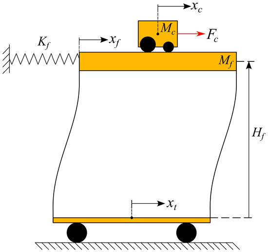
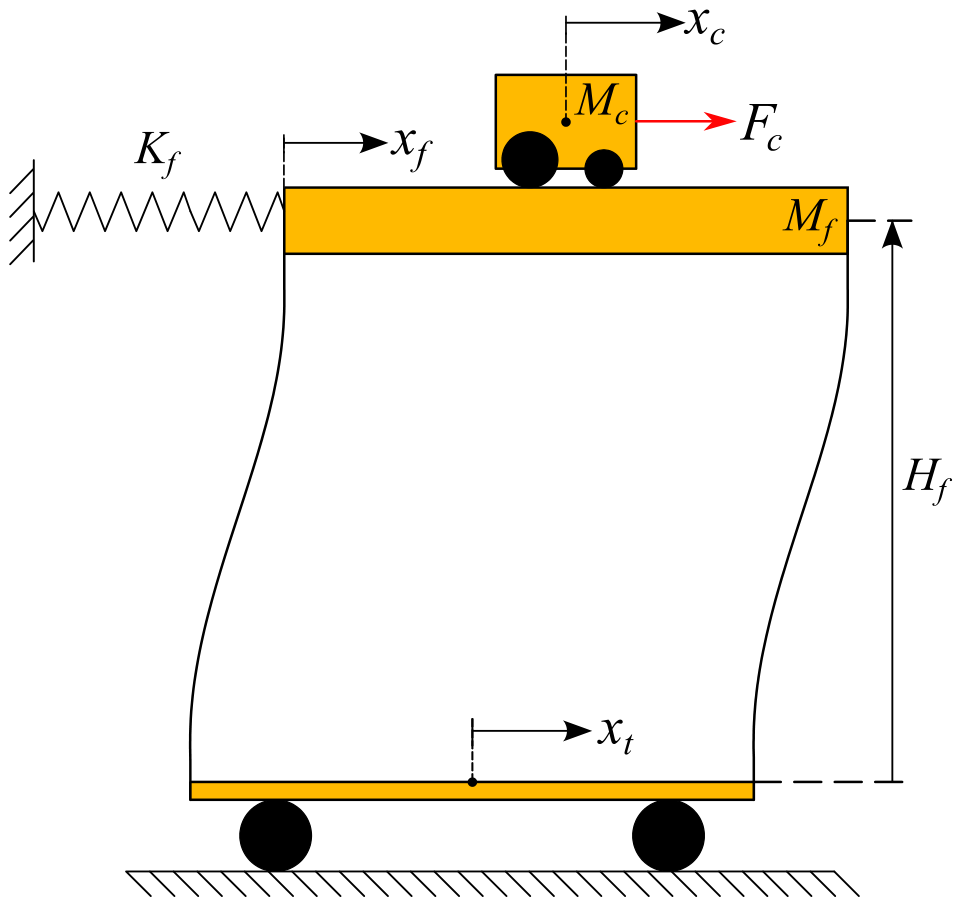
A one-story flexible structure mounted on a shake table is considered. A motor-driven AMD cart travels at floor level. The controller must reduce absolute floor displacement and acceleration without exceeding the available cart travel or actuator-voltage capability. Figure 1 shows the physical arrangement, coordinate definitions and measured signals.

Figure 1. Schematic of the shake table, one-story structure, AMD cart, coordinate definitions and available signals.

Table displacement and AMD cart travel have separate coordinates in Figure 1. This separation enables absolute floor motion, floor-to-table deformation and cart stroke to be examined separately. In particular, $x_c$ measures the rail travel available for producing the inertial control force.

All four cases use the same achieved table motion, truth model, initial state, integration step and performance definitions.

(i)

Actively centered AMD (quasi-fixed reference): A proportional-velocity loop holds the cart near the rail center. This condition approximates a fixed active mass, but it is not a mechanical clamp and it consumes electrical effort.

(ii)

Unpowered/free AMD (uncontrolled reference): The motor command is zero, while the cart mass remains on the floor and moves freely. This condition is not equivalent to removing the AMD mass.

(iii)

PP-SF: The manufacturer-provided design routine generates this fixed pole-placement state-feedback gain for the Quanser Active Mass Damper platform. The present simulation applies it with direct full-state availability. Its specified closed-loop poles are reported in Section 4.

(iv)

SMMAP-LQR: The proposed controller combines candidate-specific preview LQR laws with innovation-driven supervisory switching. Its full name is Supervisory Multiple-Model Adaptive Preview Linear Quadratic Regulator.

The four conditions separate physical and control effects. Active centering tests the structural consequence of holding the moving mass near the rail center, whereas the zero-command case exposes coupled cart-structure dynamics without commanded action. PP-SF supplies fixed active feedback and SMMAP-LQR adds model scheduling with full-record preview action. Identical plant uncertainty, excitation, initial conditions and actuator limits provide a common numerical comparison. Because PP-SF does not contain LQR weighting, preview action or supervisory scheduling, the comparison quantifies the combined SMMAP-LQR architecture and does not isolate the contribution of each component.

3. Mathematical Model

3.1. Nominal AMD-Structure Dynamics

The state vector is

$$\mathit{x}={\left[\begin{array}{cccc}{x}_c& x_f& v_c& v_f\end{array}\right]}^{\mathsf{T}}.$$

(1)

The velocity definitions are

$$v_c={\dot{x}}_c.$$

(2)

$$v_f={\dot{x}}_f.$$

(3)

Here, $x_c$ denotes cart displacement relative to the floor, $x_f$ denotes absolute floor displacement, u denotes motor voltage and $d=x_t$ denotes absolute shake-table displacement. The nominal model is

$$\dot{\mathit{x}}=A\mathit{x}+Bu+Ed.$$

(4)

The mixed coordinate definition separates the constrained AMD stroke from the structural performance variables. In particular, $x_c$ measures cart travel relative to the floor, whereas $x_f$ represents the absolute floor response. Base motion induces the relative structural deformation $x_f-x_t$; the first two state equations are purely kinematic. The state matrix is

$$A=\left[\begin{array}{cccc}0& 0& 1& 0\\ 0& 0& 0& 1\\ 0& a_{32}& a_{33}& 0\\ 0& a_{42}& a_{43}& 0\end{array}\right].$$

(5)

The input matrix is

$$B={\left[\begin{array}{cccc}0& 0& b_3& b_4\end{array}\right]}^{\mathsf{T}}.$$

(6)

The table-disturbance matrix is

$$E={\left[\begin{array}{cccc}0& 0& -a_{32}& -a_{42}\end{array}\right]}^{\mathsf{T}}.$$

(7)

The common denominator is

$$\Delta =M_c{M}_f{r}_p^2+J_m{K}_g^2(M_c+M_f).$$

(8)

The nonzero coefficients are

$$\begin{array}{cc}\hfill a_{32}& ={\displaystyle \frac{M_c{r}_p^2{K}_f}{\Delta }},\hfill \end{array}$$

(9)

$$\begin{array}{cc}\hfill a_{42}& =-{\displaystyle \frac{K_f(M_c{r}_p^2+J_m{K}_g^2)}{\Delta }},\hfill \end{array}$$

(10)

$$\begin{array}{cc}\hfill a_{33}& =-{\displaystyle \frac{(M_c+M_f)({\eta }_g{K}_g^2{\eta }_m{K}_t{K}_m+B_{eq}{R}_m{r}_p^2)}{R_m\Delta }},\hfill \end{array}$$

(11)

$$\begin{array}{cc}\hfill a_{43}& ={\displaystyle \frac{M_c({\eta }_g{K}_g^2{\eta }_m{K}_t{K}_m+B_{eq}{R}_m{r}_p^2)}{R_m\Delta }},\hfill \end{array}$$

(12)

$$\begin{array}{cc}\hfill b_3& ={\displaystyle \frac{{\eta }_g{K}_g{\eta }_m{K}_t{r}_p(M_c+M_f)}{R_m\Delta }},\hfill \end{array}$$

(13)

$$\begin{array}{cc}\hfill b_4& =-{\displaystyle \frac{M_c{\eta }_g{K}_g{\eta }_m{K}_t{r}_p}{R_m\Delta }}.\hfill \end{array}$$

(14)

Rows one and two of A give the kinematic relations. The coupled cart and floor accelerations appear in rows three and four. Floor-to-table deformation reaches both bodies through $a_{32}$ and $a_{42}$; viscous and back-EMF damping enter through $a_{33}$ and $a_{43}$. The opposite signs of $b_3$ and $b_4$ capture the reaction between the driven cart and the floor. A single denominator, $\Delta$, collects the translational masses and the motor inertia reflected through the gear train. The corresponding physical parameters are given in Table 1.

Table 1. Physical AMD-structure parameters.

Symbol	Description	Value	Unit
$M_c$	Moving cart mass	0.650	kg
$M_f$	Floor mass	1.380	kg
$K_f$	Floor stiffness at the nominal condition	500.882	N/m
$J_m$	Rotor inertia	$3.9001\times {10}^{-7}$	kg m2
$R_m$	Armature resistance	2.600	$\Omega$
$K_t$	Torque constant	0.007683	N m/A
$K_m$	Back-EMF constant	0.007678	V s/rad
$K_g$	Gear ratio	3.710	-
${\eta }_m$	Motor-side efficiency	1.000	-
${\eta }_g$	Gear-train efficiency	1.000	-
$r_p$	Pinion radius	0.00635	m
$B_{eq}$	Equivalent damping coefficient	3.000	N s/m
$T_c$	Available cart travel	0.190	m
$V_{max}$	Applied voltage bound	24.0	V
$I_{max}$	Current feasibility threshold	4.0	A

At 0.650 kg, the cart is approximately 47.1% as heavy as the floor assembly. Its inertia is large enough to provide control authority and to alter the response even when no voltage is commanded. The nominal structural mode is approximately 2.71 Hz. Although the physical rail permits 19 cm of travel, the controller monitors the tighter $\pm 8$ cm boundary to leave recovery margin. Voltage is projected directly onto the 24 V bound. Current is not saturated in the state integration; the 4 A value is checked afterward as a feasibility threshold.

At the nominal condition, the matrices evaluate to

$$A=\left[\begin{array}{cccc}0& 0& 1& 0\\ 0& 0& 0& 1\\ 0& 278.922714& -18.685723& 0\\ 0& -336.050339& 5.983113& 0\end{array}\right].$$

(15)

$$B={\left[\begin{array}{cccc}0& 0& 3.002526& -0.961400\end{array}\right]}^{\mathsf{T}}.$$

(16)

$$E={\left[\begin{array}{cccc}0& 0& -278.922714& 336.050339\end{array}\right]}^{\mathsf{T}}.$$

(17)

For $(\kappa ,\gamma )=(1,1)$, these matrices give the central member of the candidate bank. The two nonzero entries of B have opposite signs because the motor drives the cart against the floor. In E, the acceleration entries are the negatives of the stiffness column in A. Spring force thus depends on $x_f-x_t$, not on absolute floor position. A candidate model predicts floor acceleration from

$$a_f=C_a\mathit{x}+D_{a}u+F_{a}d.$$

(18)

The fourth state equation gives the output coefficients

$$C_a={\mathit{e}}_4^{\mathsf{T}}A.$$

(19)

$$D_a={\mathit{e}}_4^{\mathsf{T}}B.$$

(20)

$$F_a={\mathit{e}}_4^{\mathsf{T}}E.$$

(21)

The vector ${\mathit{e}}_4={[0,0,0,1]}^{\mathsf{T}}$ extracts ${\dot{v}}_f$ from the state derivative. Consequently, $D_a$ and $F_a$ retain the instantaneous contributions of motor voltage and table displacement. Omitting either term would make the acceleration used by the controller inconsistent with the one used to assess performance.

3.2. Scaled Earthquake Excitation

Each acceleration record is first converted to a displacement command $x_d$ and scaled to a 1.5 cm peak. The table does not follow this command ideally; its response is computed using the saturation operator

$$\mathrm{clip}(y,\ell ,h)=\min \left(\max \right(y,\ell ),h),$$

(22)

which limits y to the closed interval $[\ell ,h]$. The table acceleration is

$$a_{t,k}=\mathrm{clip}\left({\omega }_t^2(x_{d,k}-x_{t,k})-2{\zeta }_t{\omega }_t{v}_{t,k},-a_{t,\max },a_{t,\max }\right).$$

(23)

The table velocity update is

$$v_{t,k+1}=\mathrm{clip}\left(v_{t,k}+T_s{a}_{t,k},-v_{t,\max },v_{t,\max }\right).$$

(24)

The table position update is

$$x_{t,k+1}=\mathrm{clip}\left(x_{t,k}+T_s{v}_{t,k+1},-p_{t,\max },p_{t,\max }\right).$$

(25)

Equation (23) models a damped second-order position servo. Acceleration, speed and travel are clipped at their stated bounds. Since velocity is advanced before position, the two updates form a semi-implicit step. Both the structure and the preview controller receive the achieved motion $x_t$ rather than the command $x_d$. Servo tracking error remains part of every comparison. Table 2 gives the servo and integration parameters.

Table 2. Shake-table and numerical-study parameters.

Symbol	Description	Value	Unit
$T_s$	Sampling interval	0.002	s
${\zeta }_t$	Servo damping ratio	0.690107	-
${\omega }_t$	Servo natural frequency	108.5242	rad/s
$p_{t,\max }$	Table travel bound	0.021	m
$v_{t,\max }$	Table speed bound	0.416667	m/s
$a_{t,\max }$	Table acceleration bound	14.0153	m/s2
$x_{c,\lim }$	Monitored cart boundary	0.080	m
$x_{d,\mathrm{peak}}$	Peak command displacement	0.015	m

With a 2 ms interval, the table and controller update at 500 Hz. This provides about 29 samples over one cycle of the 17.27 Hz servo. Its natural frequency is approximately 6.4 times the nominal structural modal frequency, allowing the displacement command to be followed over the main structural band. The 1.5 cm command peak occupies 71.4% of the 2.1 cm table-position bound and leaves 0.6 cm of positional headroom.

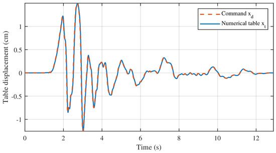
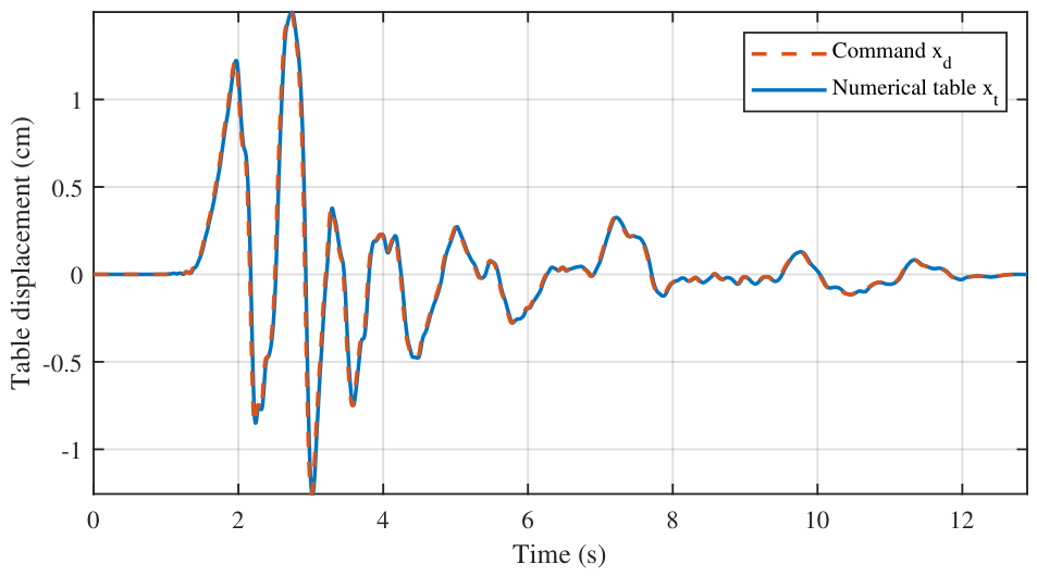
For the scaled Northridge command, Figure 2 shows close reproduction: the command and achieved peak displacements are 1.500 and 1.498 cm, respectively. The tracking error has an RMS value of 0.386 mm and a maximum value of 2.97 mm, while command-response correlation is 0.994. The achieved trajectory enters both the plant disturbance and preview calculation, so finite servo error remains part of every comparison.

Figure 2. Northridge table motion: Dashed orange scaled-displacement command and solid blue achieved servo response.

3.3. Time-Varying Nonlinear Truth Model

The truth plant differs from every linear candidate. The stiffness scale is

$$\kappa \left(t\right)={\kappa }_0+({\kappa }_1-{\kappa }_0)\mathrm{clip}(t/T_f,0,1).$$

(26)

The endpoint values are

$${\kappa }_0=0.85.$$

(27)

$${\kappa }_1=1.15.$$

(28)

Here, $T_f$ denotes the duration of the applied earthquake trajectory. The linear ramp sweeps continuously across the complete candidate stiffness range during one response calculation. Only the stiffness-dependent entries of A and E change. The actuator effectiveness is

$$B_{\gamma }=\gamma B.$$

(29)

The truth value is

$$\gamma =0.90.$$

(30)

The nonlinear truth model is

$$\dot{\mathit{x}}=A_{\kappa }\mathit{x}+B_{\gamma }u+E_{\kappa }{x}_t+\mathit{\varphi }(\mathit{x},x_t).$$

(31)

The stiffness ramp represents gradual structural variation, while $\gamma =0.90$ imposes a 10% loss of actuator effectiveness. Both variations remain inside the candidate-bank envelope, but no fixed linear candidate reproduces the complete time-varying nonlinear plant. This controlled mismatch provides the basis for testing supervisory scheduling inside a deliberately covered numerical envelope. It does not represent off-grid or out-of-range uncertainty. Write the floor deformation relative to the table as

$$\delta =x_f-x_t.$$

(32)

The hardening contribution then becomes

$$c_D=c_3{\delta }^3.$$

(33)

Cart friction is smoothed according to

$$f_c=a_c\tanh (v_c/v_s).$$

(34)

Two ratios distribute these internal forces between the cart and floor:

$${\rho }_s=-{\displaystyle \frac{A_{\kappa ,32}}{A_{\kappa ,42}}}.$$

(35)

$${\rho }_u=-{\displaystyle \frac{B_{\gamma ,4}}{B_{\gamma ,3}}}.$$

(36)

Together, the terms give

$$\mathit{\varphi }=\left[\begin{array}{c}0\\ 0\\ {\rho }_s{c}_D-f_c\\ -c_D+{\rho }_u{f}_c\end{array}\right].$$

(37)

The coefficient set used in every case is

$$c_3=2.0\times {10}^4(\mathrm{m}/{\mathrm{s}}^2)/{\mathrm{m}}^3.$$

(38)

$$a_c=0.08\mathrm{m}/{\mathrm{s}}^2.$$

(39)

$$v_s=0.01\mathrm{m}/\mathrm{s}.$$

(40)

As $\left|\delta \right|$ grows, the cubic term stiffens the structural response. The hyperbolic tangent approaches Coulomb friction smoothly and avoids a force jump at zero cart velocity. The ratios ${\rho }_s$ and ${\rho }_u$ pass both effects through the same cart-floor coupling used by the nominal model. These coefficients introduce a controlled discrepancy between the truth plant and the linear bank; they are not presented as identified hardware parameters.

4. Control Laws

4.1. Comparator Controllers

The actively centered case uses

$$u_{ctr}=-K_p{x}_c-K_v{v}_c.$$

(41)

It also uses the following position gain:

$$K_p=305.860876.$$

(42)

Lastly, it also uses the following velocity gain:

$$K_v=7.702854.$$

(43)

The large position gain keeps the cart near midstroke, while the velocity term damps its motion relative to the floor. This loop regulates the cart rather than the structural response. The stroke governor calls the same law only when the cart approaches its monitored boundary.

For the unpowered case, no terminal voltage is commanded:

$$u_0=0.$$

(44)

Zero voltage does not remove the cart or motor from the model. The cart remains free to move and its inertia stays coupled to the floor. Motor back-EMF and equivalent damping also remain in the state matrix, so the current calculation may still indicate passive electrical braking.

The fixed pole-placement state-feedback comparator (PP-SF) uses the gain generated by the manufacturer-provided design routine. Under the direct full-state assumption, its law is

$$u_{\mathrm{PP}}=-K_{\mathrm{PP}}\mathit{x}.$$

(45)

The resulting gain is

$$K_{\mathrm{PP}}=\left[\begin{array}{cccc}45.094543& -213.805044& 4.305204& -4.563960\end{array}\right].$$

(46)

The pole-placement specification sets the nominal closed-loop poles at $-6\pm 15\mathrm{j}$, $-8$ and $-16$. This PP-SF gain is distinct from the acceleration-weighted Riccati synthesis used for the SMMAP-LQR candidates.

4.2. SMMAP-LQR Candidate Bank

Let $i\in \mathcal{I}=\{1,\dots ,35\}$ index a stiffness-effectiveness pair. The stiffness candidates are

$${\kappa }_i\in \{0.85,0.90,0.95,1.00,1.05,1.10,1.15\}.$$

(47)

The effectiveness candidates are

$${\gamma }_i\in \{0.85,0.90,0.95,1.00,1.05\}.$$

(48)

Their Cartesian product yields $7\times 5=35$ candidate models. The continuous-time matrices of candidate i are

$$A_i=A_{{\kappa }_i}.$$

(49)

$$B_i={\gamma }_{i}B.$$

(50)

$$E_i=E_{{\kappa }_i}.$$

(51)

Thus, ${\kappa }_i$ changes the structural stiffness terms, whereas ${\gamma }_i$ scales the available motor authority. The grid spans a $\pm 15\%$ stiffness range and an effectiveness range from 0.85 to 1.05 in increments of 0.05; it brackets the time-varying truth model without assuming its active value.

Exact zero-order-hold discretization over one control interval gives

$$\exp \left(T_s\left[\begin{array}{ccc}{A}_i& B_i& E_i\\ 0& 0& 0\\ 0& 0& 0\end{array}\right]\right)=\left[\begin{array}{ccc}{A}_{d,i}& B_{d,i}& E_{d,i}\\ 0& 1& 0\\ 0& 0& 1\end{array}\right].$$

(52)

The sampled dynamics of candidate i are

$${\mathit{x}}_{k+1}=A_{d,i}{\mathit{x}}_k+B_{d,i}{u}_k+E_{d,i}{d}_k.$$

(53)

The augmented exponential preserves the simultaneous voltage and table- displacement inputs within each 2 ms interval. Differences among candidate predictions arise from the parameter pair rather than from different discretization approximations.

4.3. Offline Full-Record Acceleration-Weighted Preview LQR

The feedback part of each candidate uses the quadratic optimal-regulator construction, in which a Riccati equation determines the state-feedback gain for a quadratic state and input cost [52]. The stage objective is

$${\ell }_k=w_a{a}_{f,k}^2+w_f{x}_{f,k}^2+w_c{x}_{c,k}^2+w_{vc}{v}_{c,k}^2+w_{vf}{v}_{f,k}^2+w_u{u}_k^2.$$

(54)

The row selectors ${\mathit{e}}_c$, ${\mathit{e}}_f$, ${\mathit{e}}_{vc}$ and ${\mathit{e}}_{vf}$ extract $x_c$, $x_f$, $v_c$ and $v_f$, respectively, from $\mathit{x}$. The following derivation suppresses the candidate index for readability; $C_a$, $D_a$, $F_a$, Q, R, N, P and the resulting gains are evaluated separately for every candidate model. The quadratic state matrix is

$$Q=w_a{C}_a^{\mathsf{T}}{C}_a+w_f{\mathit{e}}_f^{\mathsf{T}}{\mathit{e}}_f+w_c{\mathit{e}}_c^{\mathsf{T}}{\mathit{e}}_c+w_{vc}{\mathit{e}}_{vc}^{\mathsf{T}}{\mathit{e}}_{vc}+w_{vf}{\mathit{e}}_{vf}^{\mathsf{T}}{\mathit{e}}_{vf}.$$

(55)

The input weight is

$$R=w_u+w_a{D}_a^2.$$

(56)

The state-input cross term is

$$N=w_a{C}_a^{\mathsf{T}}{D}_a.$$

(57)

The disturbance-state term is

$$q_d=w_a{C}_a^{\mathsf{T}}{F}_a.$$

(58)

The disturbance-input term is

$$r_d=w_a{D}_a{F}_a.$$

(59)

The cost places floor acceleration and displacement directly in the optimization while retaining penalties on cart stroke, cart velocity and voltage. Expanding $a_f^2={(C_a\mathit{x}+D_{a}u+F_{a}d)}^2$ produces the matrices Q, R and N together with $q_d$ and $r_d$. The disturbance-only term $w_a{F}_a^2{d}_k^2$ does not influence the minimizing voltage and is omitted from the control law. The stabilizing solution P satisfies

$$P=A_d^{\mathsf{T}}P{A}_d+Q-(A_d^{\mathsf{T}}P{B}_d+N)H^{-1}(B_d^{\mathsf{T}}P{A}_d+N^{\mathsf{T}}).$$

(60)

The scalar Hessian term is

$$H=R+B_d^{\mathsf{T}}P{B}_d.$$

(61)

The candidate feedback gain is

$$K=H^{-1}(B_d^{\mathsf{T}}P{A}_d+N^{\mathsf{T}}).$$

(62)

For each candidate, the stabilizing Riccati solution defines the feedback part of the controller. The scalar H is the effective input curvature and remains positive because the voltage penalty is positive. The resulting gain accounts for the state-input cross term introduced by direct voltage action on floor acceleration, rather than treating acceleration as a state-only output.

Following the discrete-time preview formulation and its multiple-model adaptive extension [46,47], the table servo is first simulated over the complete record to obtain $\{d_1,\dots ,d_N\}=\{x_{t,1},\dots ,x_{t,N}\}$. The affine sequence is then obtained offline through the backward recursion below. At response sample k, the supervisor uses the current state for feedback, while the stored affine term contains the remaining achieved table trajectory. The effective preview horizon is

$$N_p\left(k\right)=N-k.$$

(63)

The terminal affine state is

$$s_N=0.$$

(64)

The closed-loop adjoint matrix is

$$L=A_d^{\mathsf{T}}-(A_d^{\mathsf{T}}P{B}_d+N)H^{-1}{B}_d^{\mathsf{T}}.$$

(65)

The disturbance recursion vector is

$$g=q_d+A_d^{\mathsf{T}}P{E}_d-(A_d^{\mathsf{T}}P{B}_d+N)H^{-1}(B_d^{\mathsf{T}}P{E}_d+r_d).$$

(66)

The affine preview action is

$$f_k=-H^{-1}\left[B_d^{\mathsf{T}}{s}_{k+1}+(B_d^{\mathsf{T}}P{E}_d+r_d)d_k\right].$$

(67)

The backward recursion is

$$s_k=L{s}_{k+1}+g{d}_k.$$

(68)

The recursion runs from $k=N-1$ to $k=1$. The nominal candidate command is

$$u_{nom,k}=-K{\mathit{x}}_k+f_k.$$

(69)

The backward recursion forms the affine, disturbance-dependent part of the finite-horizon dynamic-programming solution. While $-K{\mathit{x}}_k$ regulates the current state, $f_k$ accounts for the complete remaining scaled table trajectory through $s_k$. The zero terminal condition applies to the affine term, while P retains the quadratic terminal curvature. No causal ground-motion forecast, forecast-error model or preview latency is included. The reported preview benefit therefore applies to full-record offline numerical replay rather than real-time earthquake control. Equivalently, the preview term is noncausal feedforward with respect to live earthquake operation.

4.4. Online Model Weights and Supervisory Switching

The model bank follows a supervisory multiple-model architecture in which prediction consistency governs controller selection [48,49]. Every 2 ms, each candidate forms a one-step RK4-consistent prediction. The first stage is

$${\mathit{k}}_{1,i}=A_i{\mathit{x}}_k+B_i{u}_k+E_i{d}_k.$$

(70)

The second stage is

$${\mathit{k}}_{2,i}=A_i({\mathit{x}}_k+T_s{\mathit{k}}_{1,i}/2)+B_i{u}_k+E_i(d_k+d_{k+1})/2.$$

(71)

The third stage is

$${\mathit{k}}_{3,i}=A_i({\mathit{x}}_k+T_s{\mathit{k}}_{2,i}/2)+B_i{u}_k+E_i(d_k+d_{k+1})/2.$$

(72)

The fourth stage is

$${\mathit{k}}_{4,i}=A_i({\mathit{x}}_k+T_s{\mathit{k}}_{3,i})+B_i{u}_k+E_i{d}_{k+1}.$$

(73)

The predicted next state is

$${\widehat{\mathit{x}}}_{i,k+1|k}={\mathit{x}}_k+{\displaystyle \frac{T_s}{6}}({\mathit{k}}_{1,i}+2{\mathit{k}}_{2,i}+2{\mathit{k}}_{3,i}+{\mathit{k}}_{4,i}).$$

(74)

Every candidate receives the same applied voltage and linearly interpolated table displacement over the sample. RK4 propagation matches the integration order used for the nonlinear truth plant, which limits contamination of model evidence by a lower-order predictor. At the next sample, the common measured state is compared with all stored one-step predictions. The innovation is

$${\mathit{e}}_{i,k}={\mathit{x}}_k-{\widehat{\mathit{x}}}_{i,k|k-1}.$$

(75)

Its normalized magnitude is

$${\nu }_{i,k}={\displaystyle \sum _{j=1}^4}{\left({\displaystyle \frac{e_{i,k,j}}{{\sigma }_j}}\right)}^2.$$

(76)

The robust innovation is

$${\overline{\nu }}_{i,k}=\min ({\nu }_{i,k},25).$$

(77)

The activity index is

$${\chi }_k=|x_f-x_t|+0.1|x_c|+0.005|u_{k-1}|.$$

(78)

The update gate is

$$g_k=\mathbf{1}\{{\chi }_k\ge 2\times {10}^{-4}\}.$$

(79)

Position and velocity residuals cannot be compared on their raw scales, so ${\sigma }_j$ normalizes each component before the residuals are combined. The cap at 25 prevents one nonlinear transient from discarding a candidate in a single update. When motion falls below the activity threshold, the gate holds the accumulated evidence fixed. Thus, ${\chi }_k$ is used only to decide when the weights should learn; it is not a physical energy measure. The normalized prior satisfies

$${\pi }_i\propto \exp \left[-{\displaystyle \frac{1}{2}}{\left({\displaystyle \frac{{\kappa }_i-1}{0.075}}\right)}^2-{\displaystyle \frac{1}{2}}{\left({\displaystyle \frac{{\gamma }_i-1}{0.05}}\right)}^2\right].$$

(80)

The unnormalized robust weight is

$${\tilde{p}}_{i,k}=p_{i,k-1}^{\lambda }{\pi }_i^{1-\lambda }\exp (-g_k{\overline{\nu }}_{i,k}/2).$$

(81)

Past evidence is retained with the forgetting factor

$$\lambda =0.998.$$

(82)

The normalized model weight is

$$p_{i,k}={\displaystyle \frac{\max ({\tilde{p}}_{i,k}/{\max }_j{\tilde{p}}_{j,k},{10}^{-10})}{{\sum }_{\ell }\max ({\tilde{p}}_{\ell ,k}/{\max }_j{\tilde{p}}_{j,k},{10}^{-10})}}.$$

(83)

The resulting $p_{i,k}$ values are consistency scores for choosing a controller. They are neither covariance-calibrated Bayesian probabilities nor estimates that are expected to converge to the physical parameters.

The prior assigns more weight to models near nominal stiffness and actuator authority. At each update, the forgetting factor draws old evidence gradually toward this prior, while the exponential term rewards a smaller one-step innovation. Division by the largest unnormalized weight controls numerical scale. The probability floor then keeps a temporarily poor model available in case it becomes useful later in the record.

The candidate model is

$$i_c=\arg \underset{i}{\max }{p}_{i,k}.$$

(84)

A switch from active model $i_a$ requires

$$i_c\ne i_a.$$

(85)

The dwell-time condition is

$$k-k_{sw}\ge 25.$$

(86)

The weight-ratio condition is

$$p_{i_c,k}\ge 1.20p_{i_a,k}.$$

(87)

Thus, the minimum dwell time is 0.05 s. A new model must remain eligible long enough and possess at least a 20% weight advantage before activation. The weight-ratio rule implements hysteresis in the supervisory selection [51], while the dwell time suppresses rapid controller chattering when neighboring candidates predict the measured response almost equally well. Table 3 collects the SMMAP-LQR parameters.

Table 3. SMMAP-LQR design and supervisory parameters.

Parameter	Value
Stiffness candidates ${\kappa }_i$	$0.85:0.05:1.15$
Effectiveness candidates ${\gamma }_i$	$0.85:0.05:1.05$
Number of candidate models	35
Stage weights $(w_a,w_f,w_c,w_{vc},w_{vf},w_u)$	$(1,100,5,0.5,0,0.01)$
Innovation scales $\sigma$	$(2\times {10}^{-5},2\times {10}^{-5},2\times {10}^{-3},2\times {10}^{-3})$
Innovation clipping threshold	25
Weight forgetting factor $\lambda$	0.998
Switch weight ratio	1.20
Minimum dwell time	0.05 s
Governor start and full authority	0.076 m, 0.0796 m
Voltage increment limit	5 V/update

The seven stiffness values and five effectiveness values create a 35-model bank that contains the full prescribed stiffness interval and the true effectiveness value of 0.90. This deliberate coverage tests scheduling within the defined model set rather than robustness to unrepresented plant changes. The floor-displacement weight of 100 and voltage weight of 0.01 express a vibration-suppression-oriented tradeoff, which is consistent with the increased control effort reported later. The governor starts at 7.6 cm and reaches full centering authority at 7.96 cm, immediately inside the monitored 8 cm boundary.

4.5. Stroke Governor, Voltage Projection and Actuator Monitoring

The normalized boundary coordinate is

$$z_k=\mathrm{clip}\left({\displaystyle \frac{|x_{c,k}|-x_g}{x_G-x_g}},0,1\right).$$

(88)

The smooth blending factor is

$${\beta }_k=z_k^2(3-2z_k).$$

(89)

The blended command is

$$u_k^{*}=(1-{\beta }_k)u_{nom,k}+{\beta }_k{u}_{ctr,k}.$$

(90)

The voltage-increment projection is

$${\overline{u}}_k=\mathrm{clip}(u_k^{*},u_{k-1}-5,u_{k-1}+5).$$

(91)

The voltage-amplitude projection is

$$u_k=\mathrm{clip}({\overline{u}}_k,-24,24).$$

(92)

The post-processed motor current is

$$i_k={\displaystyle \frac{u_k-(K_m{K}_g/r_p)v_{c,k}}{R_m}}.$$

(93)

The boundary coordinate is zero in the normal operating region and reaches unity close to the monitored travel limit. Its cubic smoothstep has zero slope at both endpoints, so authority transfers continuously from vibration suppression to cart centering. The subsequent projections enforce a 5 V per-update command increment and the amplifier-voltage bound.

The current expression follows the quasi-static armature balance $u=R_{m}i+K_m{\omega }_m$ with ${\omega }_m=K_g{v}_c/r_p$. Under this approximation, current is a monitored feasibility estimate and armature inductance, amplifier dynamics and thermal dynamics are outside the electrical model. The back-EMF term already contributes electromechanical damping through the state matrix; Equation (93) only reconstructs current for reporting and does not apply a second force to the plant. Voltage projection and cart governing act on the nominal unconstrained command. Only voltage amplitude and increment are directly projected. Cart travel and current are monitored quantities. The governor supplies protective centering only when its travel threshold is reached.

5. Fixed-Pair Stability Audit and Numerical Scope

The feedback stability audit uses the same 35 candidate plants, gains, sample time and exact zero-order-hold discretization as the response study. It tests individual time-invariant plant-controller assignments and is not a common-Lyapunov or multiple-Lyapunov certificate for the switched nonlinear implementation. For candidate plant p and candidate controller q, the homogeneous closed-loop matrix is

$$A_{\mathrm{cl},pq}=A_{d,p}-B_{d,p}{K}_q.$$

(94)

Its spectral radius is

$${\rho }_{pq}=\underset{\lambda \in \mathrm{eig}\left(A_{\mathrm{cl},pq}\right)}{\max }\left|\lambda \right|.$$

(95)

The corresponding linear time-invariant loop is Schur stable when

$${\rho }_{pq}<1.$$

(96)

The matched test sets $p=q$. PP-SF is evaluated separately over every candidate plant using

$$A_{\mathrm{cl},p}^{\mathrm{PP}}=A_{d,p}-B_{d,p}{K}_{\mathrm{PP}}.$$

(97)

Table 4 summarizes the resulting spectral-radius audit. All 35 matched SMMAP-LQR loops are Schur stable, with a maximum radius of 0.995584. PP-SF is also Schur stable over all 35 candidate plants and has a maximum radius of 0.989131. Across Northridge, Kobe, Imperial Valley and Cape Mendocino, the supervisor selects four unique controller settings: $(\kappa ,\gamma )=(0.95,0.90)$, $(1.00,0.90)$, $(1.00,0.95)$ and $(1.00,1.00)$. Applying these four selected gains to every candidate plant produces 140 combinations; all are Schur stable and the largest radius is 0.999573.

Table 4. Discrete-time closed-loop spectral-radius results.

Controller-Plant Set	Cases	Schur Stable	${\mathit{\rho }}_{\max }$
Matched SMMAP-LQR candidates	35	35	0.995584
Four-record selected controllers over all candidate plants	140	140	0.999573
All candidate plant-controller cross-pairings	1225	1182	1.002235
PP-SF over all candidate plants	35	35	0.989131

The 1225-pair sweep is deliberately broader than the schedule observed in the earthquake runs. It contains 43 non-Schur assignments and 1182 Schur-stable ones. The least favorable artificial pairing uses the $(1.15,0.85)$ controller with the $(0.85,1.05)$ plant, for which $\rho =1.002235$. None of these extreme assignments is needed by the realized schedule: each of the four selected controllers remains Schur stable on all 35 candidate plants. The 43 cases mark the boundary beyond that verified set.

For a plant-controller pair, preview action and table motion appear as the exogenous inputs

$${\mathit{x}}_{k+1}=A_{\mathrm{cl},pq}{\mathit{x}}_k+B_{d,p}{f}_{q,k}+E_{d,p}{d}_k.$$

(98)

If a fixed pairing is Schur stable, bounded $f_{q,k}$ and $d_k$ yield a bounded state. Its homogeneous response decays once both inputs vanish. This statement applies to the unsaturated linear candidate dynamics. It does not include the switching signal, model-weight dynamics, affine preview recursion, nonlinear truth terms, voltage projections or stroke governor. The cross-pair audit covers every gain selected in the four records, while the bounded nonlinear time histories and inactive stroke governor provide an empirical trajectory-level check. Accordingly, the analysis does not claim stability under arbitrary switching or global stability of the nonlinear constrained implementation.

6. Numerical Study Protocol

All time histories start from zero and integrate the nonlinear truth plant by RK4 with $T_s=0.002$ s. SMMAP-LQR updates its model weights and voltage command at the same numerical interval. The 2 ms step is a simulation setting rather than a verified real-time computation deadline. The model assumes direct access to the full state and uses the actuator dynamics stated above. The complete achieved table-motion sequence is available before the controlled response is calculated. The verified numerical scope does not include causal preview estimation, measurement noise, observer error, delay, quantization, amplifier dynamics or hardware timing.

The four PEER NGA acceleration records are listed in Table 5. Controller weights are set with Northridge and are not retuned for Kobe, Imperial Valley or Cape Mendocino. Acceleration samples in units of g are read at their original intervals. The manufacturer-provided earthquake scaling routine converts each acceleration history to displacement and applies coupled time and displacement scaling to produce a 1.5 cm peak table command. No separate filtering or baseline correction is applied after this routine. The complete scaled record is retained and linearly interpolated at 2 ms before the table-servo model generates the achieved displacement. The factors ${\alpha }_t=T_c/T_u$ and ${\alpha }_x=\max |X_c|/\max |X_u|$ report the resulting time and displacement scales. All records therefore share a command-displacement peak rather than a common PGA, spectral intensity or hazard level. The results characterize the four listed waveforms at this platform-oriented scale and do not constitute an intensity-scaling study.

Table 5. PEER NGA earthquake records and scaling details.

Earthquake	Station	Component	Original ${\mathit{T}}_{\mathit{s}}$ (s)	${\mathit{T}}_{\mathit{u}}$ (s)	${\mathit{T}}_{\mathit{c}}$ (s)	${\mathit{\alpha }}_{\mathit{t}}$	${\mathit{\alpha }}_{\mathit{x}}$
Northridge	Sylmar—Hospital	090	0.020	39.980	12.897	0.32259	0.08864
Kobe	HIK	000	0.020	77.980	55.298	0.70913	0.48504
Imperial Valley	El Centro Array No. 5	140	0.005	39.295	9.092	0.23138	0.04241
Cape Mendocino	Cape Mendocino	000	0.020	29.980	6.825	0.22765	0.03776

Northridge is the development record. Kobe, Imperial Valley and Cape Mendocino are evaluated without retuning. Here, $T_u$ is the duration of the imported record and $T_c$ is the duration after the manufacturer scaling routine.

The peak absolute floor displacement is

$$X_{f,pk}=100\underset{k}{\max }\left|x_{f,k}\right|.$$

(99)

The RMS absolute floor displacement is

$$X_{f,rms}=100\sqrt{N^{-1}\sum _k{x}_{f,k}^2}.$$

(100)

The relative floor displacement is

$${\delta }_k=x_{f,k}-x_{t,k}.$$

(101)

The peak floor acceleration is

$$A_{f,pk}={\displaystyle \frac{{\max }_k\left|a_{f,k}\right|}{9.81}}.$$

(102)

The RMS floor acceleration is

$$A_{f,rms}={\displaystyle \frac{\sqrt{N^{-1}{\sum }_k{a}_{f,k}^2}}{9.81}}.$$

(103)

The peak cart travel is

$$X_{c,pk}=100\underset{k}{\max }\left|x_{c,k}\right|.$$

(104)

The RMS voltage is

$$U_{rms}=\sqrt{N^{-1}\sum _k{u}_k^2}.$$

(105)

The integrated squared voltage is

$$J_u=\int u^2\mathrm{d}t.$$

(106)

Peak quantities expose the largest instantaneous demand, whereas RMS quantities measure response sustained over the entire trajectory. Absolute floor displacement quantifies motion relative to the inertial frame and ${\delta }_k$ isolates structural deformation relative to the moving table. Cart travel and voltage then show whether attenuation is achieved within the available mechanical range and voltage capability. The RMS reduction relative to PP-SF is

$$R_{rms}=100\left(1-{\displaystyle \frac{A_{f,rms}^{\mathrm{SMMAP}}}{A_{f,rms}^{\mathrm{PP}}}}\right).$$

(107)

The peak reduction relative to PP-SF is

$$R_{pk}=100\left(1-{\displaystyle \frac{A_{f,pk}^{\mathrm{SMMAP}}}{A_{f,pk}^{\mathrm{PP}}}}\right).$$

(108)

The quantity $J_u$ is a control-effort index in V²s and does not represent electrical or mechanical energy.

Positive $R_{rms}$ and $R_{pk}$ values indicate improvement over PP-SF, and the ratio form permits comparison across earthquakes with different durations and waveforms. The separate voltage-squared integral exposes stronger or more persistent commands. Electrical energy remains outside its definition because current and amplifier losses are not integrated.

7. Results and Discussion

7.1. Four-Condition Development-Record Comparison

Table 6 and Table 7 jointly report structural response and actuator demand for Northridge. The actively centered condition produces the smallest cart motion, yet its RMS floor acceleration of 0.12433 g exceeds the 0.08047 g unpowered value. Center holding is not vibration-optimal. PP-SF lowers RMS acceleration to 0.04847 g and peak acceleration to 0.34634 g. SMMAP-LQR reduces them further to 0.01297 g and 0.05656 g.

Table 6. Consolidated structural response for the Northridge earthquake.

Condition	${\mathit{X}}_{\mathit{f},\mathit{pk}}$ (cm)	${\mathit{X}}_{\mathit{f},\mathit{rms}}$ (cm)	${\mathit{\delta }}_{\mathit{pk}}$ (cm)	${\mathit{\delta }}_{\mathit{rms}}$ (cm)	${\mathit{A}}_{\mathit{f},\mathit{pk}}$ (g)	${\mathit{A}}_{\mathit{f},\mathit{rms}}$ (g)
Actively centered AMD	2.6633	0.71821	2.2935	0.54908	0.52167	0.12433
Unpowered/free AMD	2.7071	0.52815	1.9583	0.29811	0.53522	0.080471
PP-SF	2.1341	0.47670	1.5261	0.25145	0.34634	0.048474
SMMAP-LQR	1.1476	0.27299	1.0657	0.15440	0.056561	0.012974

Table 7. Consolidated AMD travel and actuator demand for the Northridge earthquake.

Condition	${\mathit{X}}_{\mathit{c},\mathit{pk}}$ (cm)	${\mathit{U}}_{\mathit{rms}}$ (V)	${\mathit{U}}_{\mathit{pk}}$ (V)	${\mathit{J}}_{\mathit{u}}$ (V2s)	${\mathit{I}}_{\mathit{rms}}$ (A)	${\mathit{I}}_{\mathit{pk}}$ (A)
Actively centered AMD	0.71564	0.55865	2.3315	4.0253	0.23304	0.97083
Unpowered/free AMD	1.5179	0	0	0	0.054208	0.35928
PP-SF	6.2988	0.73987	4.2652	7.0605	0.20061	1.1212
SMMAP-LQR	6.7652	1.1066	5.6854	15.794	0.27606	1.5625

Relative to PP-SF, SMMAP-LQR reduces RMS acceleration by 73.23%, peak acceleration by 83.67%, peak floor displacement by 46.23% and RMS floor displacement by 42.73%. It also decreases peak and RMS floor-to-table displacement from 1.5261 and 0.25145 cm to 1.0657 and 0.15440 cm, respectively. These values correspond to reductions of 30.17% and 38.59% and confirm that the improvement occurs in structural deformation as well as in absolute motion.

Peak cart travel increases by 7.40% and $J_u$ increases by 123.7%, which quantifies the additional control effort required for the improved structural response. All evaluated travel, voltage and current limits remain satisfied. The stroke governor remains inactive, so emergency center holding does not create the reported attenuation. The nonzero post-processed current in the unpowered/free condition arises from the back-EMF term in Equation (93), although its applied voltage and $J_u$ are zero. This value represents model-predicted electromechanical current rather than commanded active-control effort.

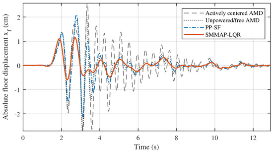
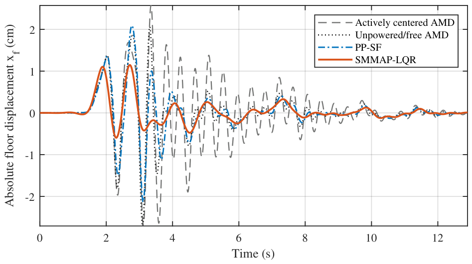
The absolute floor-displacement histories in Figure 3 place the largest excursions within the strong-motion interval. SMMAP-LQR maintains the smallest envelope around the principal peaks and during the subsequent decay. Relative to PP-SF, peak and RMS absolute displacement decrease by 46.23% and 42.73%, respectively.

Figure 3. Absolute floor-displacement histories for the four conditions.

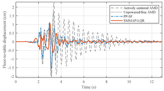
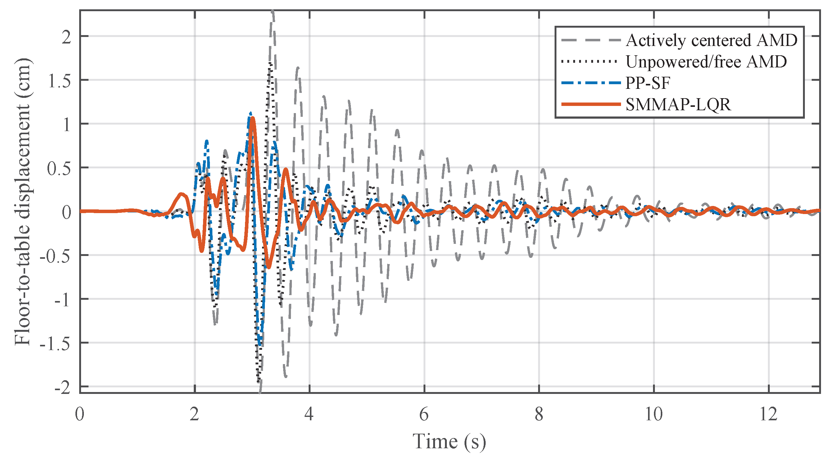
Removing common table motion from the floor coordinate preserves the response ordering in Figure 4. SMMAP-LQR produces the smallest deformation envelope, with peak and RMS reductions of 30.17% and 38.59% relative to PP-SF. Lower absolute motion is accompanied by lower structural deformation.

Figure 4. Floor displacement relative to the shake table for the four conditions.

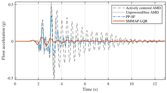
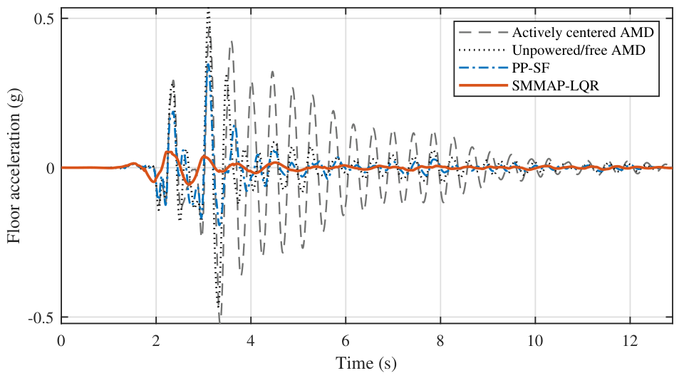
The acceleration histories in Figure 5 show that SMMAP-LQR suppresses the short-duration pulses dominating the other responses. This attenuation yields a 0.05656 g peak and 0.01297 g RMS response, equivalent to reductions of 83.67% and 73.23% from PP-SF.

Figure 5. Absolute floor-acceleration histories for the four conditions.

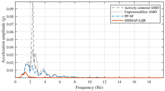
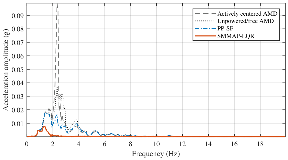
The spectral response in Figure 6 reinforces the time-domain result. The largest single-sided component decreases from 0.01814 g at 1.473 Hz for PP-SF to 0.00758 g at 1.318 Hz for SMMAP-LQR, whereas the actively centered and unpowered conditions retain larger peaks near 2.326 Hz. The 58.2% decrease in the maximum component provides frequency-domain support for the observed pulse attenuation.

Figure 6. Single-sided floor-acceleration spectra for the four conditions.

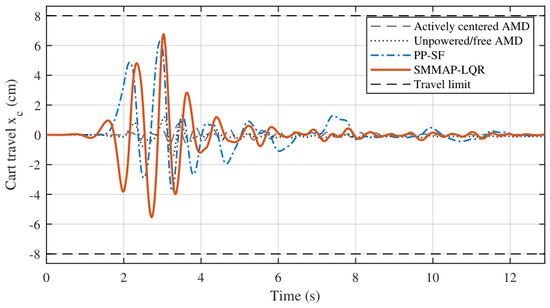
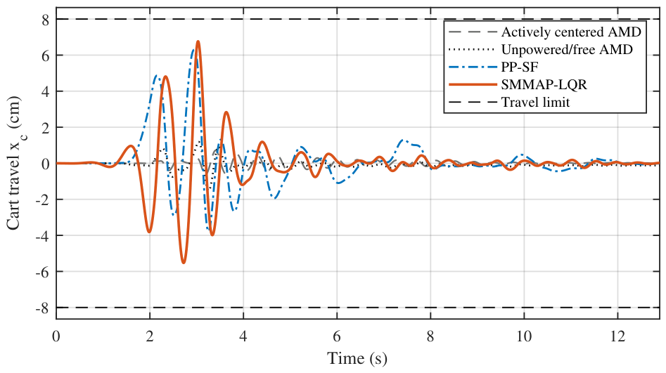
The added attenuation uses more AMD stroke than PP-SF during the main excitation, as shown in Figure 7. The 6.765 cm SMMAP-LQR peak remains inside the monitored boundary and leaves 1.235 cm of margin to the 8 cm limit.

Figure 7. AMD cart travel and the monitored $\pm 8$ cm boundary.

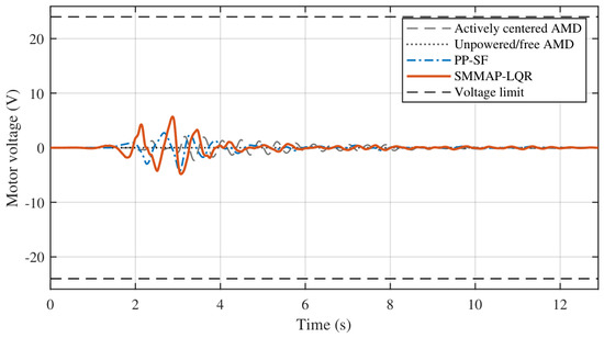
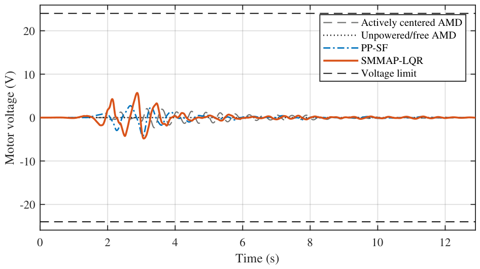
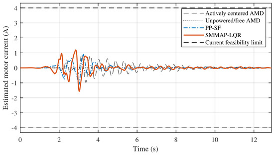
Neither active vibration controller approaches voltage saturation in Figure 8. The 5.685 V SMMAP-LQR peak uses 23.69% of the available 24 V amplitude despite its higher control effort. Relative to PP-SF, its RMS and peak voltages increase by 49.57% and 33.30%.

Figure 8. Motor-voltage histories and the enforced $\pm 24$ V limit.

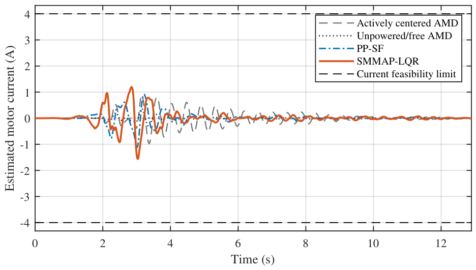
Current demand also remains below its feasibility threshold in Figure 9. The 1.5625 A SMMAP-LQR peak corresponds to 39.06% of the 4 A limit. The unpowered/free trace follows from back-EMF under a zero voltage command. Relative to PP-SF, RMS and peak current increase by 37.61% and 39.35%, quantifying the electrical cost of the added attenuation.

Figure 9. Post-processed current histories and the $\pm 4$ A feasibility threshold.

7.2. Supervisory Behavior

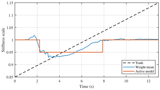
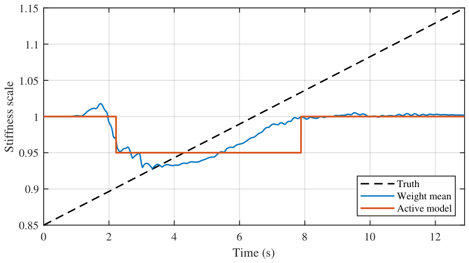
The supervisor chooses a control law rather than identifying the plant parameters. After the first 0.5 s, the stiffness weight mean has a mean absolute error of 0.0641 and a correlation of 0.487 with the true ramp; the corresponding actuator-effectiveness error is 0.0309. Five switches occur and no call to the stroke governor is made. The largest weight assigned to one model is 0.655, so the bank never collapses onto a single candidate. Under the defined nonlinear mismatch, attenuation accompanies preview action and gain scheduling. Clipped innovations, the fixed-pair spectral-radius audit and the bounded nonlinear trajectories characterize behavior only within the prescribed deterministic envelope.

Figure 10 compares quantities with different roles; it is not intended as a pointwise comparison between two stiffness estimates. The continuous ramp $\kappa \left(t\right)$ is imposed on the truth model as the prescribed stiffness variation. The weighted mean ${\overline{\kappa }}_k={\sum }_i{p}_{i,k}{\kappa }_i$ is computed from the innovation-based weights of the discrete candidate bank. The active stiffness ${\kappa }_{i_a,k}$ is the piecewise-constant candidate selected after hysteresis and dwell-time conditions are applied. Both supervisory quantities are formed from the finite model bank; neither is produced by a direct stiffness estimator. The reported error and correlation are descriptive measures of scheduling alignment with the imposed variation rather than identification accuracy. Pointwise reproduction of the continuous ramp is therefore not a control objective. The imposed ramp spans 0.85 to 1.15, while the weighted mean remains approximately between 0.93 and 1.02 and the active candidate is usually 0.95 or 1.00. Their different shapes show how a suitable controller is scheduled from aggregate prediction consistency rather than how physical stiffness is reconstructed.

Figure 10. Imposed continuous truth-model stiffness ramp, innovation-weighted candidate mean and piecewise-constant active stiffness used for gain scheduling.

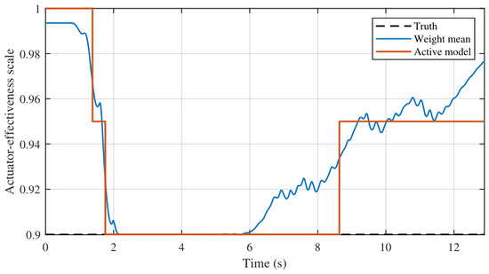
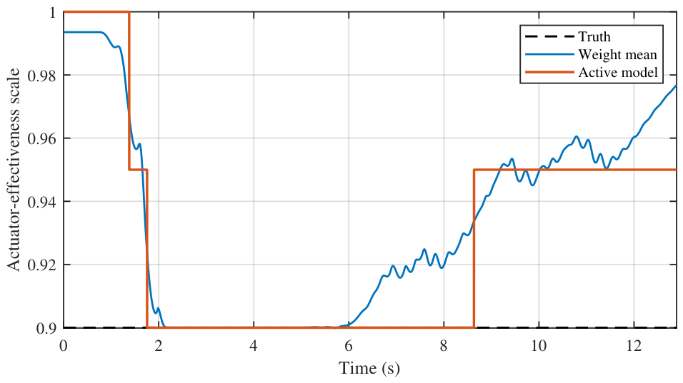
For much of the strong-motion interval in Figure 11, the selected effectiveness candidate is 0.90, which matches the truth plant. Selection moves to 0.95 as the excitation subsides. The weighted mean evolves at the same time, indicating that the bank responds to aggregate model fit rather than estimating actuator effectiveness as an isolated parameter.

Figure 11. Actuator-effectiveness scheduling: Truth-plant scale, weighted mean and active candidate.

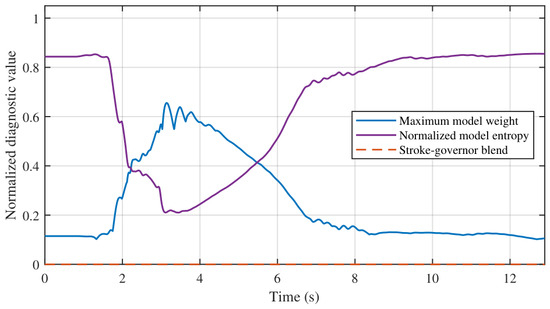
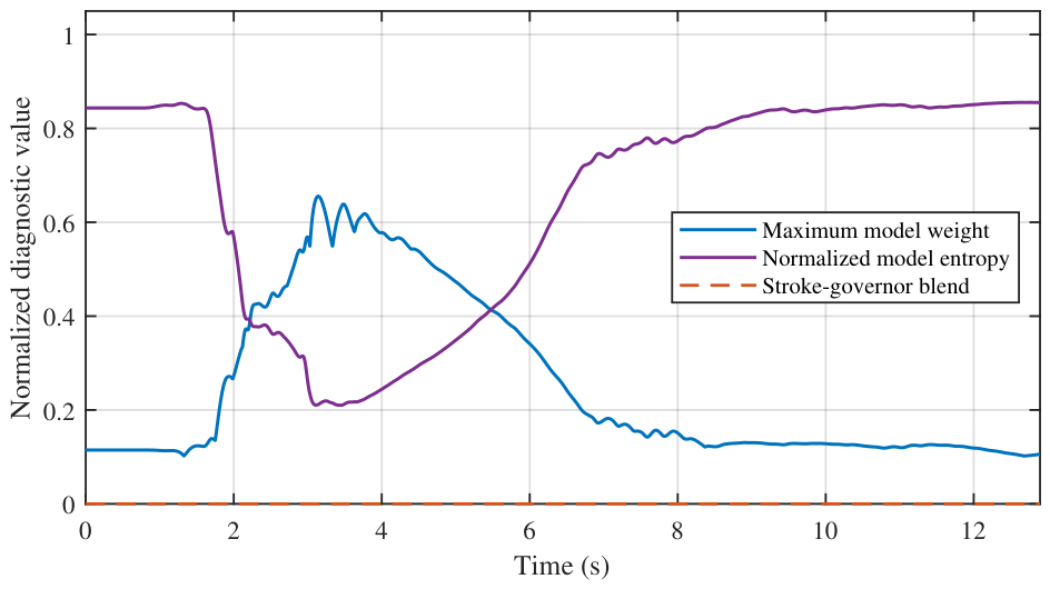
Supervisor confidence changes with the level of structural motion in Figure 12. Models separate during the main excitation and their weights spread again as the response decays. After 0.5 s, normalized entropy averages 0.648 and ranges from 0.210 to 0.855. The supervisor can thus switch without remaining locked to one candidate. Because the governor blend is identically zero, none of the reported attenuation is produced by the boundary-recovery centering law.

Figure 12. Supervisor confidence and governor activity measured by maximum model weight, normalized entropy and blend factor.

7.3. Response Across the Four Earthquakes

Table 8 places the four earthquakes side by side. The settings obtained with Northridge are carried unchanged into the other three records. Their RMS acceleration reductions remain between 65.15% and 71.28%, while the peak reductions lie between 79.58% and 81.04%. SMMAP-LQR uses 3.38–5.09 cm of peak cart travel and activates neither the cart nor the current feasibility flag.

Table 8. Consolidated cross-earthquake PP-SF and SMMAP-LQR comparison.

Earthquake	${\mathit{A}}_{\mathit{rms}}^{\mathrm{PP}}$	${\mathit{A}}_{\mathit{rms}}^{\mathit{S}}$	${\mathit{R}}_{\mathit{rms}}$ (%)	${\mathit{A}}_{\mathit{pk}}^{\mathrm{PP}}$	${\mathit{A}}_{\mathit{pk}}^{\mathit{S}}$	${\mathit{R}}_{\mathit{pk}}$ (%)	${\mathit{X}}_{\mathit{c},\mathit{pk}}^{\mathrm{PP}}$	${\mathit{X}}_{\mathit{c},\mathit{pk}}^{\mathit{S}}$	${\mathit{U}}_{\mathit{pk}}^{\mathrm{PP}}$	${\mathit{U}}_{\mathit{pk}}^{\mathit{S}}$	${\mathit{I}}_{\mathit{pk}}^{\mathit{S}}$
	(g)	(g)		(g)	(g)		(cm)	(cm)	(V)	(V)	(A)
Northridge	0.048474	0.012974	73.234	0.34634	0.056561	83.669	6.2988	6.7652	4.2652	5.6854	1.5625
Kobe	0.027626	0.0080508	70.858	0.20680	0.041441	79.960	6.1926	5.0861	2.7667	3.9634	0.9943
Imperial Valley	0.030583	0.0087827	71.282	0.15494	0.031647	79.575	5.8628	3.4769	2.2620	2.9994	0.7754
Cape Mendocino	0.030587	0.010660	65.147	0.21779	0.041283	81.044	6.1796	3.3830	2.6626	3.4664	0.9838

Unlike the Northridge development case, SMMAP-LQR requires less peak cart travel than PP-SF for every additional earthquake. The reductions are approximately 18% for Kobe, 41% for Imperial Valley and 45% for Cape Mendocino. The cross-earthquake acceleration improvements do not depend on a systematic increase in AMD stroke.

Across the four motions at the 1.5 cm displacement scale, the unchanged controller yields RMS reductions of 65.15–73.23% and peak reductions of 79.58–83.67%. Peak cart travel is lower than PP-SF in all three evaluations without retuning. This consistency extends the attenuation beyond the dominant Northridge peaks within the evaluated excitation scale. Because PP-SF uses feedback only, these reductions quantify the integrated SMMAP-LQR effect. They do not separately identify the contributions of LQR weighting, full-record preview and supervisory scheduling.

8. Conclusions

This study develops SMMAP-LQR for a numerical one-story AMD shake-table model and compares it with active center holding, zero-voltage free-cart motion and PP-SF. In the Northridge case, SMMAP-LQR lowers RMS floor acceleration by 73.23% and peak floor acceleration by 83.67% relative to PP-SF. RMS and peak floor displacement also fall by 42.73% and 46.23%, respectively. These acceleration reductions are not obtained by allowing a larger displacement response.

The additional attenuation has a measurable control cost. Peak cart travel rises by 7.40% and the voltage-squared effort index by 123.7%. Even so, the resulting 6.77 cm travel, 5.69 V voltage and 1.56 A estimated current remain within the evaluated limits. With no retuning, the other three earthquakes retain at least 65.15% RMS and 79.58% peak acceleration reduction. They also require less peak cart travel than PP-SF. The supervisory histories explain why the weights are best read as scheduling variables: the bank chooses useful controllers under aggregate mismatch rather than reconstructing each physical parameter exactly.

All 35 matched candidate loops are Schur stable. The same is true for the 140 plant-controller combinations formed from the four gains selected during the earthquake runs and the full candidate grid. In the deliberately exhaustive 1225-pair sweep, 43 extreme assignments are slightly non-Schur. Those cases locate the edge of the fixed-pair audit; they do not occur in the realized scheduling set. This audit does not establish a common Lyapunov certificate or global stability for the switched nonlinear constrained implementation.

Relative to PP-SF, the reductions arise from the combined action of acceleration-weighted full-record preview and supervisory adaptation. The present comparison does not isolate their individual effects. The verified numerical range covers four earthquake waveforms at a common 1.5 cm command scale, the defined time-varying nonlinear truth model and the stated actuator model. Across that range, SMMAP-LQR couples model-bank scheduling, offline trajectory preview, voltage projection and actuator monitoring without retuning between records. Causal preview estimation, real-time computation and experimental implementation are distinct validation steps outside the scope of the reported results.

References

- Housner, G.W.; Bergman, L.A.; Caughey, T.K.; Chassiakos, A.G.; Claus, R.O.; Masri, S.F.; Skelton, R.E.; Soong, T.T.; Spencer, B.F.; Yao, J.T.P. Structural Control: Past, Present and Future. J. Eng. Mech. 1997, 123, 897–971. [Google Scholar] [CrossRef] [Scilit]
- Spencer, B.F.; Nagarajaiah, S. State of the Art of Structural Control. J. Struct. Eng. 2003, 129, 845–856. [Google Scholar] [CrossRef] [Scilit]
- Soong, T.; Spencer, B. Supplemental energy dissipation: State-of-the-art and state-of-the-practice. Eng. Struct. 2002, 24, 243–259. [Google Scholar] [CrossRef] [Scilit]
- Koutsoloukas, L.; Nikitas, N.; Aristidou, P. Passive, semi-active, active and hybrid mass dampers: A literature review with associated applications on building-like structures. Dev. Built Environ. 2022, 12, 100094. [Google Scholar] [CrossRef] [Scilit]
- Tanveer, M.; Usman, M.; Khan, I.U.; Farooq, S.H.; Hanif, A. Material optimization of tuned liquid column ball damper (TLCBD) for the vibration control of multi-storey structure using various liquid and ball densities. J. Build. Eng. 2020, 32, 101742. [Google Scholar] [CrossRef] [Scilit]
- Banerjee, S.; Matsagar, V. Hybrid Vibration Control of Hospital Buildings against Earthquake Excitations Using Unbonded Fiber-Reinforced Elastomeric Isolator and Tuned Mass Damper. Buildings 2023, 13, 1724. [Google Scholar] [CrossRef] [Scilit]
- Kapasakalis, K.; Florakis, G.; Spanea, M.; Sapountzakis, E. Soil-Dependent Optimization of TMD- and Inerter-Based Devices for Seismic Retrofit of Multi-Story Structures. Appl. Sci. 2026, 16, 2745. [Google Scholar] [CrossRef] [Scilit]
- Weber, F. TMD-Inerter for Tall Building Damping: Approximate Closed-Form Solution, Performance and Conclusions. Buildings 2025, 15, 1829. [Google Scholar] [CrossRef] [Scilit]
- Twardoch, K.; Górski, K.; Kwiatkowski, R.; Jaśkielewicz, K.; Chiliński, B. Adaptive Pendulum-Tuned Mass Damper Based on Adjustable-Length Cable for Skyscraper Vibration Control. Sustainability 2025, 17, 6301. [Google Scholar] [CrossRef] [Scilit]
- Çağrı Sezgen, H. Hydrothermal physics based modelling and safety constrained multi objective seismic design of fluid viscous dampers. Structures 2026, 86, 111325. [Google Scholar] [CrossRef] [Scilit]
- Chang, J.C.; Soong, T.T. Structural control using active tuned mass dampers. J. Eng. Mech. Div. 1980, 106, 1091–1098. [Google Scholar] [CrossRef] [Scilit]
- Hrovat, D.; Barak, P.; Rabins, M. Semi-Active versus Passive or Active Tuned Mass Dampers for Structural Control. J. Eng. Mech. 1983, 109, 691–705. [Google Scholar] [CrossRef] [Scilit]
- Samali, B.; Yang, J.N.; Liu, S.C. Active Control of Seismic-Excited Buildings. J. Struct. Eng. 1985, 111, 2165–2180. [Google Scholar] [CrossRef] [Scilit]
- Dyke, S.J.; Spencer, B.F.; Quast, P.; Sain, M.K. Role of Control-Structure Interaction in Protective System Design. J. Eng. Mech. 1995, 121, 322–338. [Google Scholar] [CrossRef] [Scilit]
- Battaini, M.; Yang, G.; Spencer, B.F. Bench-Scale Experiment for Structural Control. J. Eng. Mech. 2000, 126, 140–148. [Google Scholar] [CrossRef] [Scilit]
- Zhang, C.; Ou, J. Control Structure Interaction of Electromagnetic Mass Damper System for Structural Vibration Control. J. Eng. Mech. 2008, 134, 428–437. [Google Scholar] [CrossRef] [Scilit]
- Casciati, S.; Chen, Z. An active mass damper system for structural control using real-time wireless sensors. Struct. Control Health Monit. 2012, 19, 758–767. [Google Scholar] [CrossRef] [Scilit]
- Rincon, C.; Alencastre, J.; Rivera, R. Analytical Modelling of an Active Vibration Absorber for a Beam. Mathematics 2023, 11, 2009. [Google Scholar] [CrossRef] [Scilit]
- Quanser Inc. Active Mass Damper. 2026. Available online: https://www.quanser.com/products/active-mass-damper/ (accessed on 11 August 2026).
- Zhang, C.; Ning, L.; Mohammadzadeh, A. Experimental Investigation on an Innovative Stable and Online Trained Type-3 Fuzzy Controller for Structural Vibrations. Soil Dyn. Earthq. Eng. 2026, 200, 109898. [Google Scholar] [CrossRef] [Scilit]
- Miyamoto, K.; She, J.; Sato, D.; Yasuo, N. Automatic determination of LQR weighting matrices for active structural control. Eng. Struct. 2018, 174, 308–321. [Google Scholar] [CrossRef] [Scilit]
- Çağrı Sezgen, H. Design of an Active Tuned Mass Damper (ATMD) and Simulation for Vibration Reduction in Multi-Degree-of-Freedom Systems. In Proceedings of the 2025 International Conference on Control, Automation and Instrumentation (IC2AI), Beirut, Lebanon, 11–13 February 2025; pp. 1–6. [Google Scholar] [CrossRef] [Scilit]
- Alvarez, P.; McElwain, B.; Thesing, L.; Edalath, S.; Kukreti, A.; Cohen, K. PD and fuzzy logic control for earthquake resilient structures. Comput. Appl. Eng. Educ. 2014, 22, 142–152. [Google Scholar] [CrossRef] [Scilit]
- Guclu, R.; Yazici, H. Vibration control of a structure with ATMD against earthquake using fuzzy logic controllers. J. Sound Vib. 2008, 318, 36–49. [Google Scholar] [CrossRef] [Scilit]
- Al-Dawod, M.; Samali, B.; Li, J. Experimental verification of an active mass driver system on a five-storey model using a fuzzy controller. Struct. Control Health Monit. 2006, 13, 917–943. [Google Scholar] [CrossRef] [Scilit]
- Nagashima, I.; Shinozaki, Y. Variable gain feedback control technique of active mass damper and its application to hybrid structural control. Earthq. Eng. Struct. Dyn. 1997, 26, 815–838. [Google Scholar] [CrossRef]
- Chen, C.J.; Li, Z.H.; Teng, J.; Wu, Q.G.; Lin, B.C. A variable gain state-feedback technique for an AMD control system with stroke limit and its application to a high-rise building. Struct. Des. Tall Spec. Build. 2021, 30, e1816. [Google Scholar] [CrossRef] [Scilit]
- Materazzi, A.L.; Ubertini, F. Robust structural control with system constraints. Struct. Control Health Monit. 2012, 19, 472–490. [Google Scholar] [CrossRef] [Scilit]
- Zhang, S.; Li, Q.; Zhao, X.; Liu, Z.; Li, G. Vibration Control for an Active Mass Damper of a High-Rise Building with Input and Output Constraints. IEEE/ASME Trans. Mechatron. 2023, 28, 186–196. [Google Scholar] [CrossRef] [Scilit]
- Mayne, D.; Rawlings, J.; Rao, C.; Scokaert, P. Constrained model predictive control: Stability and optimality. Automatica 2000, 36, 789–814. [Google Scholar] [CrossRef] [Scilit]
- Bemporad, A.; Morari, M.; Dua, V.; Pistikopoulos, E.N. The explicit linear quadratic regulator for constrained systems. Automatica 2002, 38, 3–20. [Google Scholar] [CrossRef] [Scilit]
- Feng, J.; Liu, Z.; He, X.; Fu, Q.; Li, G. Adaptive Vibration Control for an Active Mass Damper of a High-Rise Building. IEEE Trans. Syst. Man Cybern. Syst. 2022, 52, 1970–1983. [Google Scholar] [CrossRef] [Scilit]
- Gao, H.; Hu, J.; Qi, Y.; Sun, C. Adaptive vibration control of a flexible structure based on hybrid learning controlled active mass damping. J. Frankl. Inst. 2022, 359, 5935–5959. [Google Scholar] [CrossRef] [Scilit]
- Saleem, O.; Filograno, M.L.; Alharbi, S.; Iqbal, J. Hierarchical Fuzzy-Adaptive Position Control of an Active Mass Damper for Enhanced Structural Vibration Suppression. Mathematics 2025, 13, 2816. [Google Scholar] [CrossRef] [Scilit]
- Zhang, C.; Pei, S.; Mohammadzadeh, A. Deep online learning type-3 fuzzy structural control strategy for active vibration suppression: Real-world validation. Int. J. Dyn. Control 2025, 13, 423. [Google Scholar] [CrossRef] [Scilit]
- Zhang, C.; Pei, S.; Mohammadzadeh, A. An Adaptive-switching Fuzzy Structural Vibration Control System: Theory and Experiment. J. Vib. Eng. Technol. 2025, 13, 309. [Google Scholar] [CrossRef] [Scilit]
- Zhang, C.; He, S.; Mohammadzadeh, A. A Novel Vibration Control System for Active Mass Drivers Based on Dynamic Fractional-order Type-2 Fuzzy Model and Adaptive Fractional Derivative. J. Vib. Eng. Technol. 2025, 13, 553. [Google Scholar] [CrossRef] [Scilit]
- Li, Q.; Zhang, S.; Zhao, X.; Liu, Z.; He, W.; Li, G. Adaptive Neural Network Event-Triggered Control for a High-Rise Building with Active Mass Damper. IEEE Trans. Syst. Man Cybern. Syst. 2025, 55, 8251–8260. [Google Scholar] [CrossRef] [Scilit]
- Jia, S.; Ouyang, Y.; Wu, H.; Kou, X.; Li, Y. Data-driven design of vibration control with active mass damper. J. Phys. Conf. Ser. 2025, 2977, 012015. [Google Scholar] [CrossRef] [Scilit]
- Gao, H.; He, W.; Zhang, Y.; Sun, C. Vibration Control based on Reinforcement Learning for a Flexible Building-like Structure System with Active Mass Damper against Disturbance Effects. In Proceedings of the 2020 59th IEEE Conference on Decision and Control (CDC), Jeju Island, Republic of Korea, 14–18 December 2020; pp. 2380–2385. [Google Scholar] [CrossRef] [Scilit]
- Zhang, Y.A.; Ke, S.; Zhu, S. Model-free active vibration control based on imitation learning and deep reinforcement learning: Experimental implementation in an SDOF structure. Smart Mater. Struct. 2026, 35, 035009. [Google Scholar] [CrossRef] [Scilit]
- Zhang, Y.; Ma, G.; Wu, G.; Li, L. Modeling and nonlinear optimal control of active mass damper with rotating actuator for structural vibration control. Struct. Control Health Monit. 2022, 29, e2871. [Google Scholar] [CrossRef] [Scilit]
- Larbi, S.H.; Bourahla, N.; Benchoubane, H.; Choutri, K.; Badaoui, M. Earthquake Ground Motion Matching on a Small Electric Shaking Table Using a Combined NN-PDFF Controller. Shock Vib. 2020, 2020, 7260590. [Google Scholar] [CrossRef] [Scilit]
- Liu, J.; Silva, C.E.; Dyke, S.J.; Wu, Y.; Liu, H. Using real-time hybrid simulation for active mass damper experimentation and validation. Mech. Mach. Theory 2024, 191, 105474. [Google Scholar] [CrossRef] [Scilit]
- Tomizuka, M. Optimal continuous finite preview problem. IEEE Trans. Autom. Control 1975, 20, 362–365. [Google Scholar] [CrossRef] [Scilit]
- Katayama, T.; Ohki, T.; Inoue, T.; Kato, T. Design of an optimal controller for a discrete-time system subject to previewable demand. Int. J. Control 1985, 41, 677–699. [Google Scholar] [CrossRef] [Scilit]
- Wang, D.; Liao, F.; Tomizuka, M. Adaptive preview control for piecewise discrete-time systems using multiple models. Appl. Math. Model. 2016, 40, 9932–9946. [Google Scholar] [CrossRef] [Scilit]
- Morse, A. Supervisory control of families of linear set-point controllers—Part I. Exact matching. IEEE Trans. Autom. Control 1996, 41, 1413–1431. [Google Scholar] [CrossRef] [Scilit]
- Narendra, K.; Balakrishnan, J. Adaptive control using multiple models. IEEE Trans. Autom. Control 1997, 42, 171–187. [Google Scholar] [CrossRef] [Scilit]
- Hespanha, J.; Liberzon, D.; Morse, A.S.; Anderson, B.D.O.; Brinsmead, T.S.; Bruyne, F.D. Multiple model adaptive control. Part 2: Switching. Int. J. Robust Nonlinear Control 2001, 11, 479–496. [Google Scholar] [CrossRef] [Scilit]
- Hespanha, J.P.; Liberzon, D.; Morse, A.S. Hysteresis-based switching algorithms for supervisory control of uncertain systems. Automatica 2003, 39, 263–272. [Google Scholar] [CrossRef] [Scilit]
- Ogata, K. Modern Control Engineering, 5th ed.; Prentice Hall: Boston, MA, USA, 2010. [Google Scholar]
Disclaimer/Publisher’s Note: The statements, opinions and data contained in all publications are solely those of the individual author(s) and contributor(s) and not of MDPI and/or the editor(s). MDPI and/or the editor(s) disclaim responsibility for any injury to people or property resulting from any ideas, methods, instructions or products referred to in the content. |
© 2026 by the authors. Licensee MDPI, Basel, Switzerland. This article is an open access article distributed under the terms and conditions of the Creative Commons Attribution (CC BY) license.