


Abstract
As power systems continue to expand and grow in complexity, power flow calculation remains a fundamental task in power system analysis and operation. Conventional methods rely on iterative solvers and detailed grid models, yet are often hindered by non-convergence and unreliable modeling assumptions. To address these limitations, this paper introduces a deep learning-based approach that integrates graph neural networks (GNNs) and recurrent neural networks (RNNs) for power flow calculation. The proposed model captures spatial dependencies through graph convolutional layers and temporal dynamics through recurrent layers, enabling accurate prediction of node voltage magnitudes, phase angles, and branch power flows. To enhance transparency, SHAP (Shapley Additive exPlanations)-based feature attribution and multi-modal visualizations are employed to interpret the model’s predictions. Experimental results on the IEEE 9-bus, 39-bus, and 118-bus systems demonstrate prediction errors within 4% and a computational speedup of approximately 40-fold over traditional Newton–Raphson methods. Beyond technical performance, these results suggest that the proposed method can support more efficient and reliable grid operation, thereby contributing to the integration of renewable energy, enhancement of grid resilience, and advancement of sustainable energy systems.
Keywords:
power flow calculation; deep learning; graph neural network; data-driven; interpretability MSC:
68T07; 93C95
1. Introduction
The power system is a cornerstone of modern society, supporting daily life, industrial production, and commercial activities [1]. Among its many analytical tasks, power flow calculation is a central concern in electrical engineering [2] and has attracted extensive research attention. Its primary objective is to determine the voltage, current, and power distribution at different nodes across the system [3], thereby providing critical insights into the stability, reliability, and operation of power networks [4,5].
The study of traditional power flow calculation methods began with the application of the Newton–Raphson algorithm [6]. In recent years, researchers have made substantial efforts to enhance these classical approaches. For example, Montoya and Gil-González proposed a numerical analysis method based on successive approximations to address power flow problems in AC distribution systems [7]. In another effort, the Newton–Raphson method was combined with homotopy continuation to create an improved variant that reduces computational errors and accelerates convergence, thereby contributing to the safe and stable operation of power systems and supporting the appropriate selection of electrical equipment [8]. Moreover, advanced optimization techniques such as the enhanced alternating direction method of multipliers (ADMM) and the augmented Lagrangian-based alternating direction inexact Newton (ALADIN) method have been applied to solve optimal power flow (OPF) problems in distributed or multi-area AC grids [9]. Additionally, Ghasemi et al. [10] explored the use of an evolutionary-based approach, namely the hybrid modified imperialist competitive algorithm (MICA) and teaching–learning algorithm (MICA–TLA), to optimize OPF control variables. However, despite these advancements, traditional methods still cannot fully overcome their inherent limitations. In particular, their modeling capacity remains constrained when addressing the nonlinear and highly complex characteristics of modern power systems.
As power systems continue to expand and electricity demand increases, the complexity of power flow calculation also grows, bringing new challenges to conventional approaches:
Complex network topology: Modern power systems often consist of hundreds or even thousands of nodes and transmission lines, forming highly intricate network structures [11]. The computational burden of traditional methods rises sharply with system size, as their complexity scales exponentially with the number of nodes, leading to prohibitively long computation times in large-scale systems [12,13].
Nonlinear characteristics: Power systems include numerous components such as generators, transformers, and transmission lines, all of which exhibit strong nonlinear behaviors. These nonlinearities are difficult for conventional linearization-based methods to capture accurately, thereby limiting their ability to model the dynamic characteristics of real systems [14].
Data noise and uncertainty: Power system data is often affected by uncertainties such as load fluctuations and line losses. Traditional methods generally lack robustness to such noisy data, which reduces the accuracy and reliability of their power flow calculations [15].
In light of these challenges, deep learning technologies have emerged as powerful tools with strong potential to enhance both the precision and efficiency of power flow calculations [16,17]. Pan et al. [18] introduced a deep neural network (DNN) framework to address uncertainties arising from renewable generation and flexible load patterns, achieving a significant reduction in computation time compared to traditional iterative solvers. Fioretto et al. [19] developed a deep learning methodology for OPF computation, leveraging the dual Lagrangian method to ensure compliance with inherent physical and engineering constraints. Another investigation [20] unveiled a DNN method operating within a so-called “preventive” framework, which consistently demonstrates accelerated performance under both light and heavy load conditions. Furthermore, Singh et al. [21] advocated for the training of a sensitivity-informed DNN (SI-DNN); findings from this work conclusively show that the OPF solutions predicted by SI-DNN outperform those derived from conventionally trained DNNs. Additionally, Lei et al. [22] proposed a physics-informed machine learning approach for data-driven optimal power flow, which integrates physical constraints into neural network training to ensure physically consistent predictions. Beyond fully connected networks, researchers have increasingly turned to graph-based architectures. Donon et al. [23] proposed an innovative artificial neural network architecture based on graph neural networks, where the graph neural solver autonomously learns instead of attempting to replicate the output of the Newton–Raphson solver. Additionally, Lopez-Garcia and Domínguez-Navarro [24] presented a method for power flow analysis via typed graph neural networks, integrating node and branch type information into the message-passing framework to enhance representation quality. Cao et al. [25] introduced a physics-informed graphical representation for robust voltage control in distribution systems. Gao et al. [26] proposed a physics-guided graph convolutional neural network for optimal power flow, demonstrating the effectiveness of integrating physical constraints into graph-based learning. More recently, Ghamizi et al. [27] developed SafePowerGraph, a safety-oriented benchmarking framework for GNNs in transmission grids, demonstrating that graph attention architectures and self-supervised learning significantly improve model robustness under adversarial operational scenarios. In parallel, transformer-based architectures have also been explored for power system applications. Chen et al. [28] proposed Powerformer, a section-adaptive Transformer for power flow adjustment that integrates transmission section information into the attention mechanism, achieving superior performance on systems with up to 9241 buses. Furthermore, Ezeakunne et al. [29] introduced a physics-informed graph attention network with continual learning capability, enabling a single model to generalise across 13 benchmark systems while maintaining prediction errors below 1%, thus demonstrating the potential of attention-based GNNs for large-scale, multi-system power flow analysis [30].
In summary, the preceding review reveals three key observations. First, deep learning methods—particularly GNNs and, more recently, attention-based architectures—have demonstrated substantial promise in power flow and OPF applications, consistently outperforming traditional iterative solvers in speed while maintaining competitive accuracy [16,17,23,24,27,28,29,30]. Second, despite this progress, the majority of existing data-driven approaches address either spatial topology modelling (via GNNs) or temporal load dynamics (via sequence models) in isolation; few studies have systematically integrated both dimensions within a unified framework. Third, the interpretability of deep learning models in power systems remains underexplored. Although SHAP-based methods have emerged as the dominant XAI technique in energy applications [31,32], their use in power flow calculation has been largely qualitative, lacking the quantitative rigour required for operational decision-making.
To address these gaps, this paper proposes a hybrid deep learning framework that jointly models spatial grid topology through graph neural networks and temporal load dynamics through recurrent neural networks, augmented by a comprehensive SHAP-based interpretability analysis. The novelty of this work is threefold: (i) it is the first study, to the best of our knowledge, to integrate GNN and RNN components within a single architecture for steady-state power flow calculation, enabling simultaneous capture of spatial and temporal dependencies; (ii) it provides a quantitative SHAP-based feature attribution analysis that links model predictions to physically meaningful electrical parameters, moving beyond qualitative interpretation; and (iii) it validates the proposed framework across three IEEE benchmark systems of increasing scale, establishing a reproducible baseline for future research in interpretable deep learning for power systems. The main contributions are as follows:
- A hybrid GNN–RNN architecture for power flow analysis that jointly captures spatial topology through graph convolutional layers and temporal dynamics through recurrent layers, achieving accurate predictions of node voltages, phase angles, and branch power flows.
- Integration of grid topology as an explicit input via the adjacency matrix, enabling the model to learn connectivity-aware representations that go beyond conventional node-level feature engineering.
- A comprehensive interpretability framework combining SHAP-based feature attribution with multi-modal visualizations (time-series trend plots, heatmaps, and node/branch status diagrams), providing actionable insights into how electrical parameters and topological features influence power flow predictions.
- Extensive validation across three IEEE benchmark systems (9-bus, 39-bus, and 118-bus), demonstrating approximately 40-fold computational speedup over traditional Newton–Raphson methods while maintaining prediction errors within 4%.
The remainder of this paper is organized as follows: Section 2 introduces data processing and feature engineering; Section 3 details the principles of power flow analysis, model construction, and interpretability methods; Section 4 presents three case studies to validate the proposed approach; and Section 5 concludes the work.
2. Data Processing and Feature Engineering
Power system power flow analysis is a fundamental task within electrical engineering, encompassing intricate network topologies and diverse electrical parameters. This section presents a comprehensive treatment of power system data management for power flow analysis, covering data preprocessing, feature engineering, and data standardization, followed by an in-depth discussion of the selected input features and target variables relevant to power flow calculations.
2.1. Data Preprocessing
Power flow analysis relies on large volumes of data collected from diverse sources, including monitoring equipment, sensors, and real-time measurement systems.
The efficacy of deep learning is closely tied to the dataset size and training approach, necessitating a substantial volume of load data for each power grid node. In this study, data were collected for n distinct load nodes, each sampled at K distinct time instances representing different load conditions. These datasets encompass load node sequences, active power flow matrices, reactive power flow matrices, as well as node voltage magnitudes and phase angles, all obtained through rigorous load flow calculations.
Prior to analysis, the raw datasets were subjected to a standardized preprocessing pipeline [33]. The following three procedures were applied, with their selection driven by the physical characteristics of power system data and the requirements of deep learning models.
First, outliers and noise in the load-flow results were detected using a three-sigma () statistical criterion applied to node voltage magnitudes and branch power flows. The rule was chosen because steady-state power system measurements typically follow an approximately Gaussian error distribution under normal operating conditions, and the method is non-parametric, requiring no pre-labelled anomaly dataset. Data points exceeding the thresholds were regarded as anomalies and replaced with interpolated values to preserve temporal consistency.
Second, missing entries, which primarily resulted from incomplete measurements at specific time instances, were handled by applying zero-filling for inactive nodes and linear interpolation for continuous variables such as voltage and power. Linear interpolation was selected over alternatives such as forward-filling or mean imputation because it preserves the temporal continuity inherent in physical quantities, avoiding the introduction of artificial discontinuities that could degrade gradient-based model training.
Third, all numerical features—including voltage magnitudes, phase angles, and active/reactive power values—were normalized using min–max scaling to the range . Min–max normalization was preferred over Z-score standardisation because it preserves the non-negative nature of physical quantities such as voltage magnitudes and power values, maps features to a bounded interval compatible with the output range of commonly used activation functions (e.g., sigmoid and ReLU), and is more stable than Z-score when feature distributions are bounded rather than unbounded. This normalization procedure was applied consistently across both training and testing datasets to eliminate scale disparities, thereby improving model stability and convergence during training.
2.2. Feature Engineering
In power flow analysis, the selection of input features is of fundamental importance, as these features exert a direct influence on model performance and predictive accuracy. In this study, the feature selection process is guided by key physical and operational characteristics of the power system. Specifically, voltage magnitude and phase angle are incorporated to represent the electrical states of nodes, providing essential information on both the strength and phase relationship of node voltages. Branch parameters, including resistance, reactance, and admittance, are also considered, as they govern current flow and significantly affect transmission losses. In addition, load data is employed to reflect the demand imposed on the system, thereby capturing critical aspects of grid stability and load distribution. Finally, active and reactive power setpoints of generators are included as control variables, since they play a decisive role in determining system operation and ensuring the reliable balance between generation and demand.
Taking these data features into account, and recognizing that real-world power grids are primarily affected by real-time load fluctuations that induce flow perturbations, variations in node voltages are relatively limited. Instead, real-time variations predominantly manifest in node load levels, which exert a substantial influence on the outcomes of power flow analysis. Moreover, given the diversity of node types within the grid (source, load, and bus nodes), load levels provide a relatively consistent and intuitive metric for evaluating changes in system states. Hence, this paper primarily selects the active power load sequence P, reactive power load sequence Q, voltage magnitude V, voltage phase angle , as well as the impedance R, admittance I of the branches, and active power output , reactive power output of the generators at PQ nodes and balanced nodes in the power system as the numerical input features for the deep learning model. The complete feature set is denoted as:
Node-level data features alone are insufficient to capture the full complexity of power grid characteristics. To address this limitation, the interconnection information among grid nodes—namely, the topological relationships—is incorporated to construct a topological representation of the power grid. By leveraging the grid topology, spatial features between nodes are derived, represented by the adjacency matrix , which encodes the connectivity of the power grid. Here, each element of denotes the connection status between node i and node j: a value of 1 signifies a connection, while 0 indicates otherwise. The node feature matrix and the adjacency matrix then serve as the two primary inputs to the graph neural network, jointly representing the electrical states and structural connectivity of the grid.
Furthermore, to enhance the modelling of the power grid’s dynamic behavior and evolving states, temporal data is also incorporated as an additional learning objective [34]. The time-series feature matrix and the node feature matrix jointly constitute the input to the recurrent neural network, allowing the model to capture both the temporal evolution and the instantaneous electrical states of the grid.
Feature engineering constitutes a pivotal step in power system data processing, as it not only involves the extraction of numerical features but also incorporates spatial and topological characteristics of the grid. To enhance the efficiency and accuracy of model training, this study implements a series of structured feature engineering techniques.
First, the data is reorganized into a three-dimensional array, where each sample corresponds to a node, each column represents a feature, and each layer denotes a time step. This structure enables the model to capture spatial relationships within temporal data. Second, correlation matrices are computed for the features of each sample, facilitating the extraction of interdependencies among different variables. Third, Laplacian graphs are constructed to explicitly represent topological links between nodes, thereby assisting the model in learning connectivity patterns within the power grid.
In practical applications, power flow analysis often yields sparse power flow matrices, reflecting the fact that not all nodes are directly interconnected. To improve computational efficiency and reduce the number of training parameters, the power flow matrix is preprocessed by eliminating dimensions with values equal to or near zero.
Based on these considerations, the proposed model is designed with input dimensions corresponding to the total number of features across all nodes and time steps, encompassing load data, topological information, and the results of power flow calculations. The corresponding output dimension is , where e denotes the number of effective edges in the grid topology and m represents the number of load and balance nodes in the system.
By integrating these feature engineering methods, the study substantially improves the utilization of power system data for load flow analysis and prediction, enabling both enhanced computational efficiency and predictive performance.
2.3. Construction of Output Target Variables
In the context of load flow analysis for power systems, the determination of output features requires a careful selection of parameters that exert a direct impact on both electrical quality and overall system stability [35]. Accordingly, this study designates as target variables the key electrical parameters of nodes and branches derived from load flow analysis results for each bus within the system. The prediction and analysis of these target variables hold substantial significance in assessing power system stability, load distribution, fault diagnosis, and operational planning. The primary target variables of interest in this study are listed as follows:
Node voltage magnitudes characterize the electrical potential at individual nodes of the power system. Maintaining these values within an acceptable range is essential for ensuring system stability and preventing equipment damage, as abnormal voltage magnitudes can trigger instability or failures. The voltage magnitude of the i-th node is denoted as .
Node phase angles describe the relative phase relationships among node voltages, directly influencing the distribution of current and power flows across the system. Preserving consistent phase relationships is critical for maintaining balance and synchrony. The phase angle of the i-th node is expressed as .
Branch active power flow reflects the transfer of real power across network branches. Accurate estimation of active power is critical for load distribution and power balance in the power system. denotes the active power on the branch between the i-th and j-th nodes.
Branch reactive power flow represents the transmission of reactive power between nodes, which plays a pivotal role in voltage regulation and system stability. Effective allocation of reactive power is necessary for ensuring proper power factor and voltage balance. The reactive power on the branch between the i-th and j-th nodes is denoted as .
Collectively, these target variables serve as critical indicators of the performance and stability of the power system. Accurate prediction enables real-time monitoring, early detection of potential risks, and the formulation of corrective strategies, thereby enhancing the reliability and efficiency of power system operation. The integration of deep learning techniques further strengthens this process by capturing complex nonlinear dependencies among the variables, leading to improved accuracy and robustness in load flow analysis.
3. Electric Power System Load Flow Analysis Principles and Deep Learning Applications
This section first introduces the fundamental principles of load flow analysis in power systems, then describes the deep learning models and network architectures employed in this study, and finally explains how the GNN and RNN components are integrated to achieve accurate power flow predictions.
3.1. Principles of Traditional Load Flow Analysis
Load flow analysis is a fundamental task in power system engineering, providing essential information on voltage, current, and power at various nodes of the system. These parameters are crucial for system planning, operation, and control.
At the heart of load flow analysis lies the node voltage equations, a critical set of equations in power system analysis used to describe the relationship between the voltages and powers at different nodes within the system. These equations are typically expressed in complex form and encompass relationships between power injection, loads, branch parameters, and node voltages. In practice, each node in the system is associated with a voltage value and a complex power value, consisting of both active (real) and reactive power. The general form of the node voltage equations can be expressed as:
where represents the complex power injected at node i; is the magnitude of the voltage at node i; is the current vector injected at node i; m is the number of nodes connected to node i; is the admittance between node i and node j; is the magnitude of the voltage at node j; and is the phase angle of the voltage at node j.
The node current is determined by the node voltage and the admittance, where admittance represents the complex characteristics of branch parameters, including resistance and reactance. The primary purpose of the node voltage equation is to compute the voltage at each node for subsequent power flow calculations. In power flow calculations, when the voltage and loads at certain nodes are known, it is necessary to calculate the voltage and power at other nodes. This equation is typically used in conjunction with power flow calculation methods such as the Newton–Raphson method to determine the voltage and power at various nodes in the power system.
For traditional power flow analysis methods, the Newton–Raphson method is primarily employed to solve the power flow equations [11]. For an electric power system consisting of m nodes, the power flow equations can be formulated as follows:
where and denote the active and reactive power output of the generator at node i, respectively; and represent the active and reactive loads connected to node i, respectively; and are the negative values of the admittance (conductance and susceptance) between node i and node j; and are the voltage magnitudes of node i and node j, respectively; and is the voltage angle difference, where .
3.2. Deep Learning Design and Applications
3.2.1. Data-Driven Framework for Power Flow Analysis
For deep learning-based power flow analysis, the execution process of the GNN–RNN framework is summarized in Table 1. The procedure begins with the construction of historical load sequences for the nodes, along with the connectivity information describing inter-node relationships. From these load sequences, the corresponding voltage and power flow output data are obtained, while the system topology is simultaneously derived and stored in a data repository for subsequent processing.
Table 1.
Execution procedure of GNN–RNN.
In the second stage, the network is trained using the collected datasets. During this process, a constraint is imposed to exclude power flow matrix entries corresponding to zero line power, which indicates the absence of physical transmission lines. This ensures that the model parameters are learned solely from meaningful electrical connections.
Finally, in the third stage, real-time load sequences and the network topology are input into the pre-trained model to conduct rapid power flow analysis. This enables the network to generate fast and accurate predictions of node-level power flow outputs, thereby enhancing the efficiency of real-time power system analysis.
3.2.2. Deep Learning Network Design
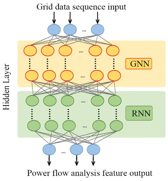
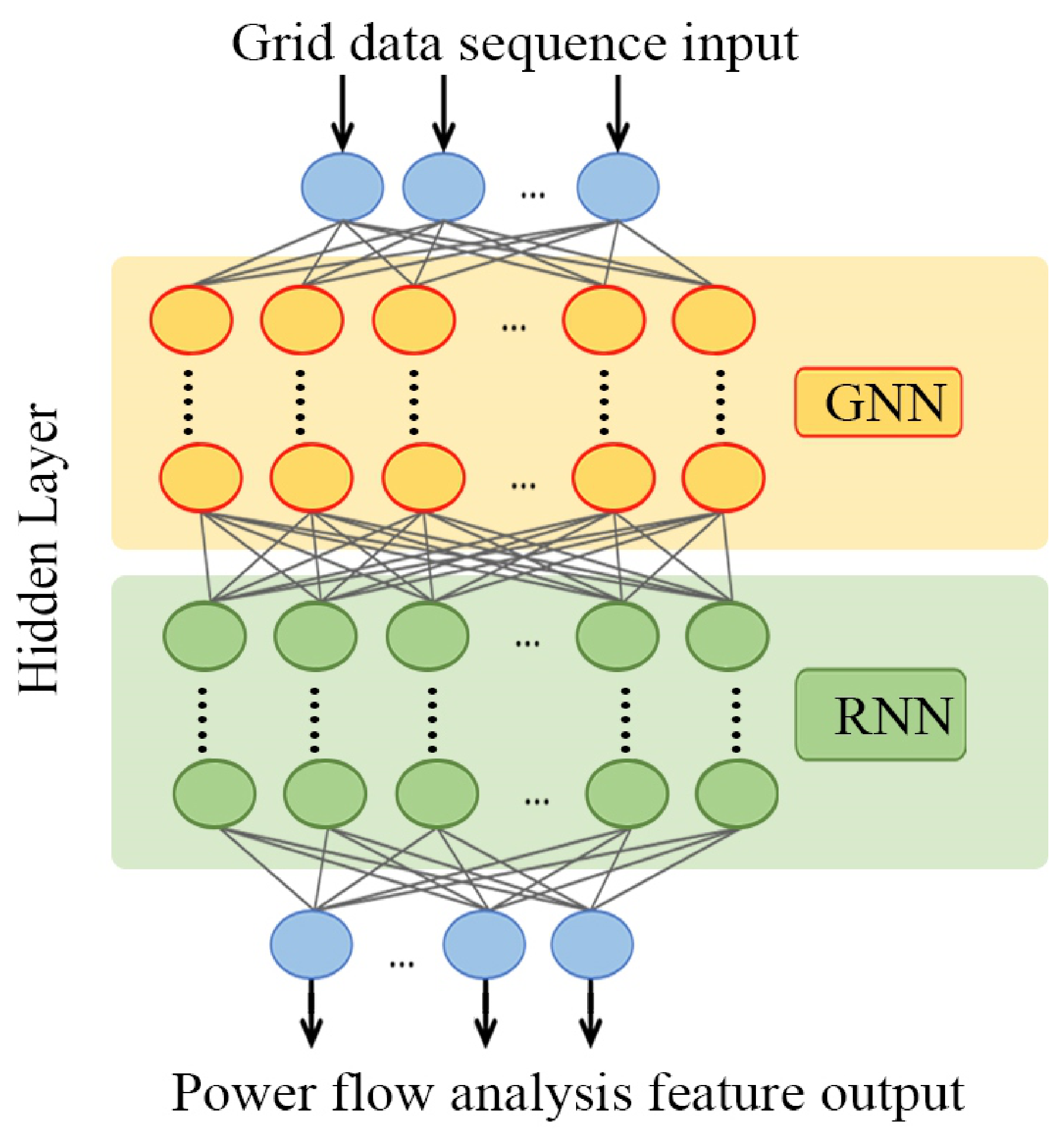
The overall network architecture, illustrated in Figure 1, comprises an input layer, multiple hidden layers, and an output layer. The hidden layer structure adopted in this study integrates two key components: a GNN and a RNN. This design enables the model to effectively capture both the topological dependencies among nodes and the temporal dynamics of load variations within the power system.
Figure 1.
Network design diagram.
To enhance model robustness, dropout regularization is applied to the fully connected layer, mitigating the risk of overfitting and improving generalization performance. The subsequent subsections provide a detailed explanation of the design principles and functional roles of the two hidden layer structures employed in this framework.
3.2.3. Graph Neural Network (GNN)
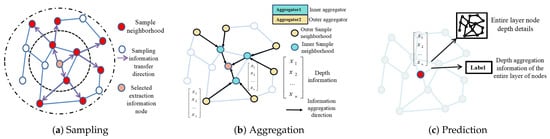
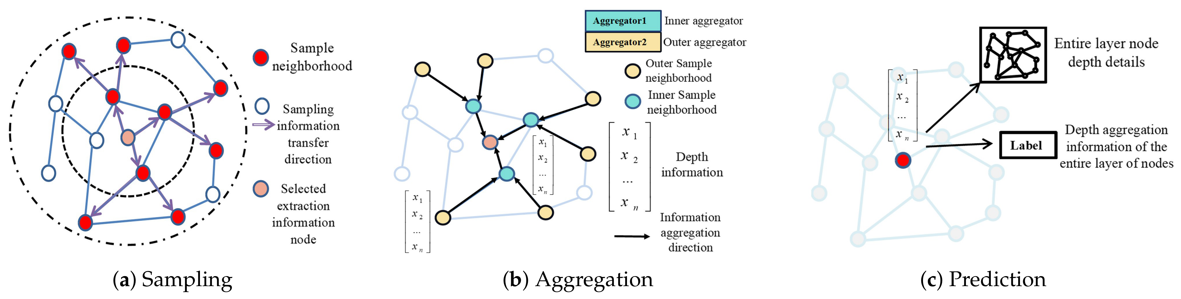
In this study, the GNN component is constructed with two GraphSageConv layers, which are classical graph convolutional layers designed for structured data. The underlying operation is illustrated in Figure 2. The purpose of this network is to enable efficient propagation and aggregation of information among nodes, thereby capturing the topological dependencies of the power system [36].
Figure 2.
Principle diagram of GraphSageConv network.
The GNN takes as input an adjacency matrix, which encodes the topological relationships among nodes in the power system. This matrix has dimensions (number of nodes × number of nodes), effectively representing the electrical grid’s connectivity. The basic update rule of GraphSAGE can be expressed as [36]:
where is the node representation at layer k-th; and are learnable parameters; is the activation function; AGGREGATE is a permutation-invariant aggregation function (e.g., mean or max pooling).
To capture the graph structure, the graph Laplacian is employed:
where is the degree matrix and is the adjacency matrix. Based on the Laplacian, a local pooling filter can be defined as:
where is the identity matrix; and are hyperparameters, and is the graph Laplacian.
The final output of the GNN is obtained by flattening and passing through a fully connected layer:
where Flatten denotes the vectorization operation, and Dense represents the fully connected layer.
In practice, this study applies two GraphSageConv layers to perform iterative information propagation, thereby allowing the network to learn both local and global dependencies among nodes in the power grid. The feature dimensions are set to 128 for the first layer and 64 for the second layer, with the ReLU function serving as the activation mechanism. For the aggregation function, the mean aggregator is adopted, which computes the element-wise mean of neighbour embeddings. The mean aggregator was selected because it provides stable gradient flow during training and treats all neighbouring nodes equally—a design choice that aligns with the physical symmetry of power grid connections, where no single adjacent bus is inherently more important than another prior to learning. The number of neighbouring nodes sampled per layer is set to for the first GraphSAGE layer and for the second layer: the first layer samples a larger neighbourhood to capture broad local topology, while the second layer samples a smaller set to refine the representation. This design enables effective extraction of spatial features, ensuring that the learned representations capture the underlying structural patterns of the power system.
In Figure 2a, the red-highlighted nodes represent sampled neighbours that provide local neighbourhood information to the target node. Moving to Figure 2b, the aggregation process is illustrated with two levels: Aggregator 2 (outer layer aggregator) first collects depth information from the outer neighborhood and passes it inward, while Aggregator 1 (inner-layer aggregator) integrates both inner-neighborhood data and the information received from the outer layer. This hierarchical aggregation ensures that the target node captures multi-level structural dependencies. Finally, as shown in Figure 2c, the aggregated information is transmitted to the target node, allowing the model to form a depth-enhanced representation of the entire layer.
This process corresponds directly to the GraphSAGE formulation introduced earlier: the correlation matrix encodes the topological connections between nodes, while the aggregation functions enable the network to iteratively combine features across different neighborhood depths. By incorporating this mechanism, the proposed model effectively captures multi-hop relational dependencies in the power grid, thereby enhancing its ability to represent and predict node-level power flow characteristics.
3.2.4. Recurrent Neural Network (RNN)
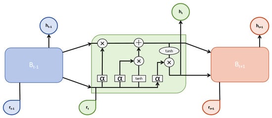
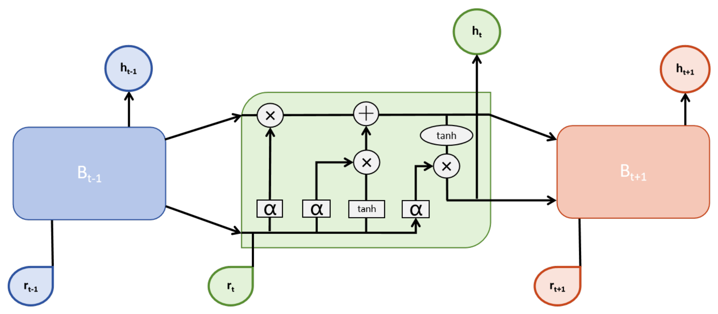
Long Short-Term Memory (LSTM) is a widely adopted RNN structure for modeling time-series data [37,38]. Its architecture is illustrated in Figure 3. In this study, the RNN component processes historical time-series data, capturing temporal dependencies among various parameters in the power system [39]. Two LSTM layers are employed: the first with an output feature dimension of 128, and the second with an output feature dimension of 32. These stacked LSTM layers enhance the network’s ability to capture both short-term and long-term temporal patterns in power system dynamics.
Figure 3.
LSTM network unit structure diagram.
The operations of the LSTM can be described step by step as follows [39]:
First, the forget gate determines how much of the previous cell state should be retained:
where is the weight matrix; is the previous hidden state; is the current input; is the bias term; and is the sigmoid activation function.
Next, the input gate regulates the amount of new information added to the cell state:
The candidate cell state is then updated using the hyperbolic tangent function:
where tanh is the hyperbolic tangent activation function.
The output gate is expressed as:
The cell state update is given by:
The hidden state is given by:
The mean squared error (MSE) loss is defined as:
where is the true label and is the predicted label. The parameters are updated using backpropagation with gradient descent:
where is a model parameter; is the learning rate; and is the gradient of the loss with respect to the parameter.
Although a single steady-state power flow calculation depends only on the boundary conditions of the current time step, power systems in practice operate under continuously varying load conditions where adjacent time steps exhibit strong temporal correlations. Capturing these temporal dependencies allows the model to learn richer representations of the grid’s dynamic behavior. Moreover, for optimal power flow over a planning horizon, the coupling across time steps becomes explicit through generator ramping constraints and intertemporal costs. Therefore, incorporating RNNs into the proposed framework enables the model to exploit these temporal patterns, improving both prediction accuracy and robustness under realistic operating scenarios.
3.2.5. Feature Fusion and Architecture Summary
The GNN and RNN branches produce complementary representations: the GNN output (Equation (8)) captures spatial dependencies derived from the grid topology, while the final hidden state of the LSTM (Equation (14)) encodes temporal dynamics from the load sequences. These two representations are concatenated to form a joint spatial–temporal feature vector:
where ‖ denotes vector concatenation. The fused vector is then passed through a fully connected layer with ReLU activation, followed by a final linear output layer to produce the predicted node voltages, phase angles, and branch power flows. Dropout (rate = 0.3) is applied before the final layer to mitigate overfitting. The complete forward pass proceeds as follows:
- The node feature matrix and adjacency matrix are fed into the GNN branch (two GraphSageConv layers → flatten → dense) to produce .
- The time-series feature matrix and node features are fed into the RNN branch (two LSTM layers) to produce the final hidden state .
- and are concatenated into .
- is passed through a fully connected layer (ReLU) and a linear output layer to yield the final predictions.
Table 2 summarises the complete architecture, listing the input and output dimensions of each component for the three test systems.
Table 2.
Architecture summary of the proposed GNN–RNN model.
3.2.6. Design of Interpretability Methods for Results
Interpretability has become increasingly critical in deep learning and machine learning, particularly in high-stakes domains such as healthcare, finance, and energy [40,41,42]. In the context of power system load flow calculations, accurately understanding model predictions and decision-making processes is of paramount importance. Interpretability contributes in several key ways: it clarifies how predictions are derived from input features, thereby strengthening trust and comprehension of model outputs; it helps identify errors or biases under specific scenarios, thus improving model robustness and accuracy [43]; and it facilitates clearer communication of the model’s mechanisms and rationale to users and stakeholders, enhancing credibility and acceptance. Moreover, interpretability provides valuable guidance for subsequent model refinement, offering insights into model behavior that enable targeted adjustments to structure and parameters for improved performance.
Interpretability methods address the inherent opacity of deep learning models, which are often regarded as “black boxes” with internal mechanisms that are difficult to elucidate [44]. This limitation is particularly critical in the power systems domain, where decision-makers must understand how predictions are derived before acting on them. By making the model’s reasoning transparent, interpretability techniques enhance the credibility and practical applicability of deep learning for power system load flow analysis.
This study adopts SHAP values as the interpretability method. SHAP values, rooted in cooperative game theory, quantify the contribution of individual features to model predictions by considering all possible permutations of feature values and their average marginal effects. Assuming a predictive model f with an input feature vector and an output result , for a specific sample , this study aims to discern the influence of each feature on the output .
The computation of SHAP values proceeds as follows: for a given model prediction , each feature is systematically introduced into a feature subset S, and the model’s prediction is evaluated for this modified subset [45]. The marginal contribution of is then defined as the change in the model’s prediction when is added to S. The computational formula is:
Here, represents the SHAP value of feature i, where f denotes the model’s prediction function. N signifies the set of all features, while S represents a subset of features. indicates the model’s prediction result corresponding to the feature subset S, and represents the model’s prediction result after incorporating feature i into the feature subset S.
To further enhance interpretability, this study incorporates visual representations of model outputs, ensuring that the predictive results can be more clearly understood. The time-series output trend plot displays the model’s predicted values over time, with time on the horizontal axis and predictions on the vertical axis, allowing for the identification of predictive trends and periodic patterns. In addition, node and branch status diagrams are employed to illustrate the operating conditions of the power system, where node diagrams typically depict voltage magnitudes and phase angles, while branch diagrams reflect power flow characteristics. Heatmaps are also utilized to provide an intuitive overview of node and branch statuses, with color gradients representing magnitudes such as node voltage or branch power flow. Through these visualization techniques, the model’s outputs can be effectively communicated, thereby deepening the understanding of both predictive performance and system operation. When combined with the SHAP interpretability method, these visualizations further enable comprehensive insights into the model’s predictions and the underlying processes that drive them.
4. Experiments and Results Analysis
4.1. Dataset and Model Parameter Configuration
To evaluate the effectiveness of the proposed method, comprehensive experiments were conducted using multiple benchmark power system datasets. All data used in this study are simulated, generated from three classic IEEE test systems: the IEEE 9-bus, IEEE 39-bus, and IEEE 118-bus systems [46]. The standard IEEE test case data provided the base load values, network topology, and line parameters for each system.
4.2. Data Generation Procedure
The training datasets were constructed through the following procedure. First, the base active and reactive load values at each load bus were taken from the standard IEEE test case specifications. To simulate realistic load variations over time, random perturbations were applied to the base load of each node independently. Specifically, at each time step t, the load at node i was set as:
where and denote the base active and reactive loads at node i, and is a random perturbation factor drawn independently from a uniform distribution for each node and each time step. This perturbation range was selected to represent moderate-to-severe load fluctuations while remaining within the operational limits of each test system. The independence of perturbations across nodes ensures that the dataset covers a wide variety of spatially heterogeneous loading conditions.
For each perturbed load configuration, a full AC power flow calculation was performed using the Newton–Raphson method to obtain the ground-truth values of node voltage magnitudes, phase angles, and branch active and reactive power flows. Each such calculation constitutes one sample in the dataset. The temporal granularity was set to 20 min, corresponding to typical SCADA measurement intervals in real power systems.
This procedure was repeated to generate over 10,000 samples per system, covering a period of approximately four to five months of simulated operation. Dataset 1 is derived from the IEEE 9-bus system, while Dataset 2 and Dataset 3 correspond to the IEEE 39-bus and 118-bus systems, respectively. For each dataset, samples were partitioned into training, validation, and test sets in a 70/15/15 ratio, ensuring that all subsets span the full range of loading conditions. These three datasets capture time-series information and topological connections for various nodes in the power system. Details of the training parameters and network configuration are presented in Table 3.
Table 3.
Network parameters for different systems.
4.3. Model Training
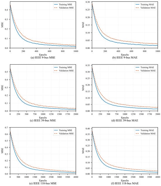
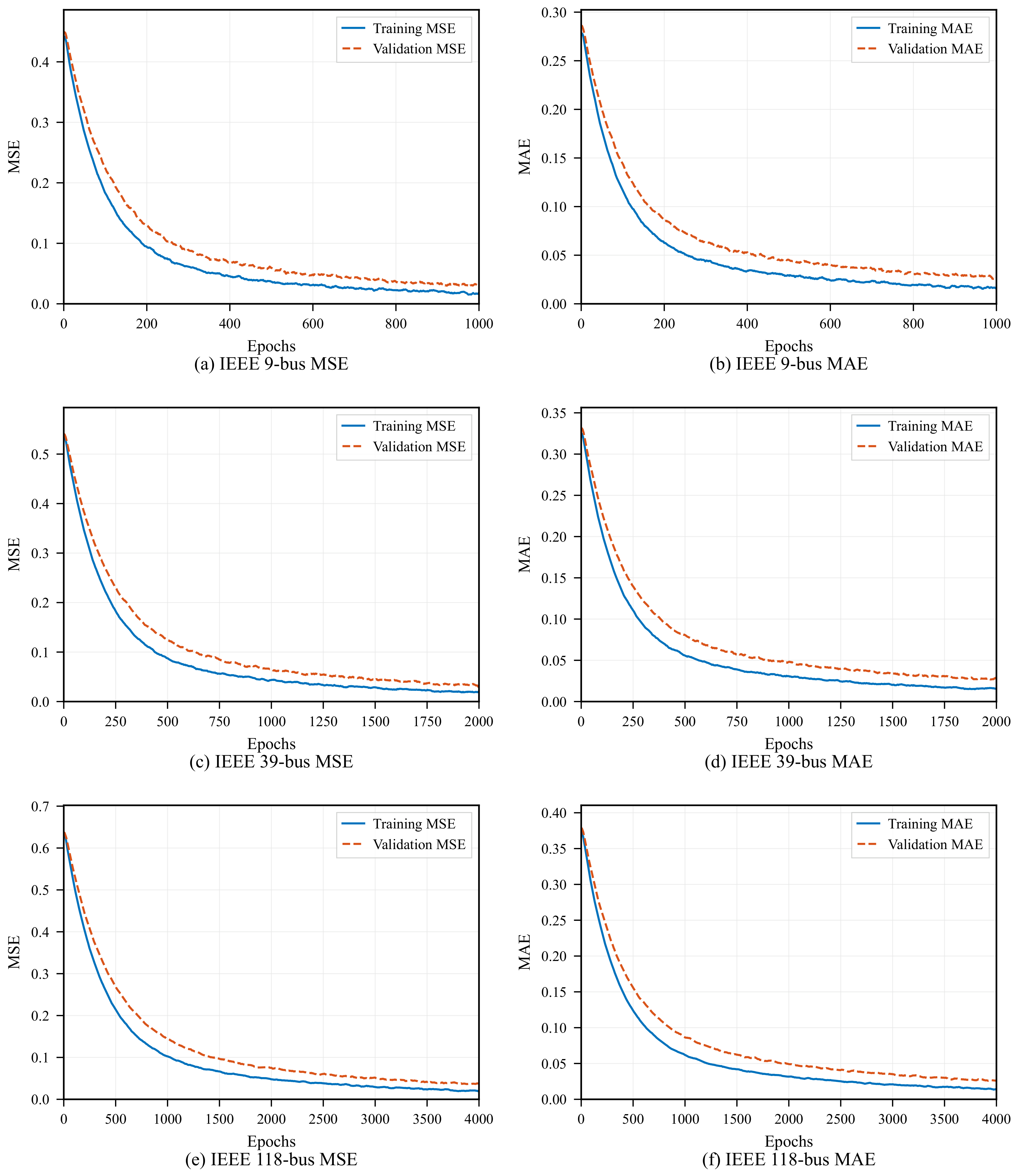
In the training process, the Mean Squared Error (MSE) is employed as the loss function. Furthermore, the Mean Absolute Error (MAE) is calculated to provide a comprehensive evaluation of the model’s predictive performance. The loss function training curves for the predictive model on the three datasets are illustrated in Figure 4.
Figure 4.
Model loss function and performance evaluation: (a) MSE loss on IEEE 9-bus system; (b) MAE on IEEE 9-bus system; (c) MSE loss on IEEE 39-bus system; (d) MAE on IEEE 39-bus system; (e) MSE loss on IEEE 118-bus system; (f) MAE on IEEE 118-bus system. Solid blue curves denote training loss, and dashed orange curves denote validation loss.
In Figure 4, both the MSE and MAE exhibit a pronounced downward trend across training iterations, indicating effective optimization of the predictive model. The consistent decline of both metrics on the validation set further demonstrates that the model generalizes well to unseen data, rather than merely memorizing the training samples.
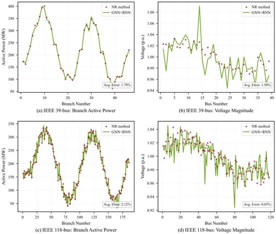
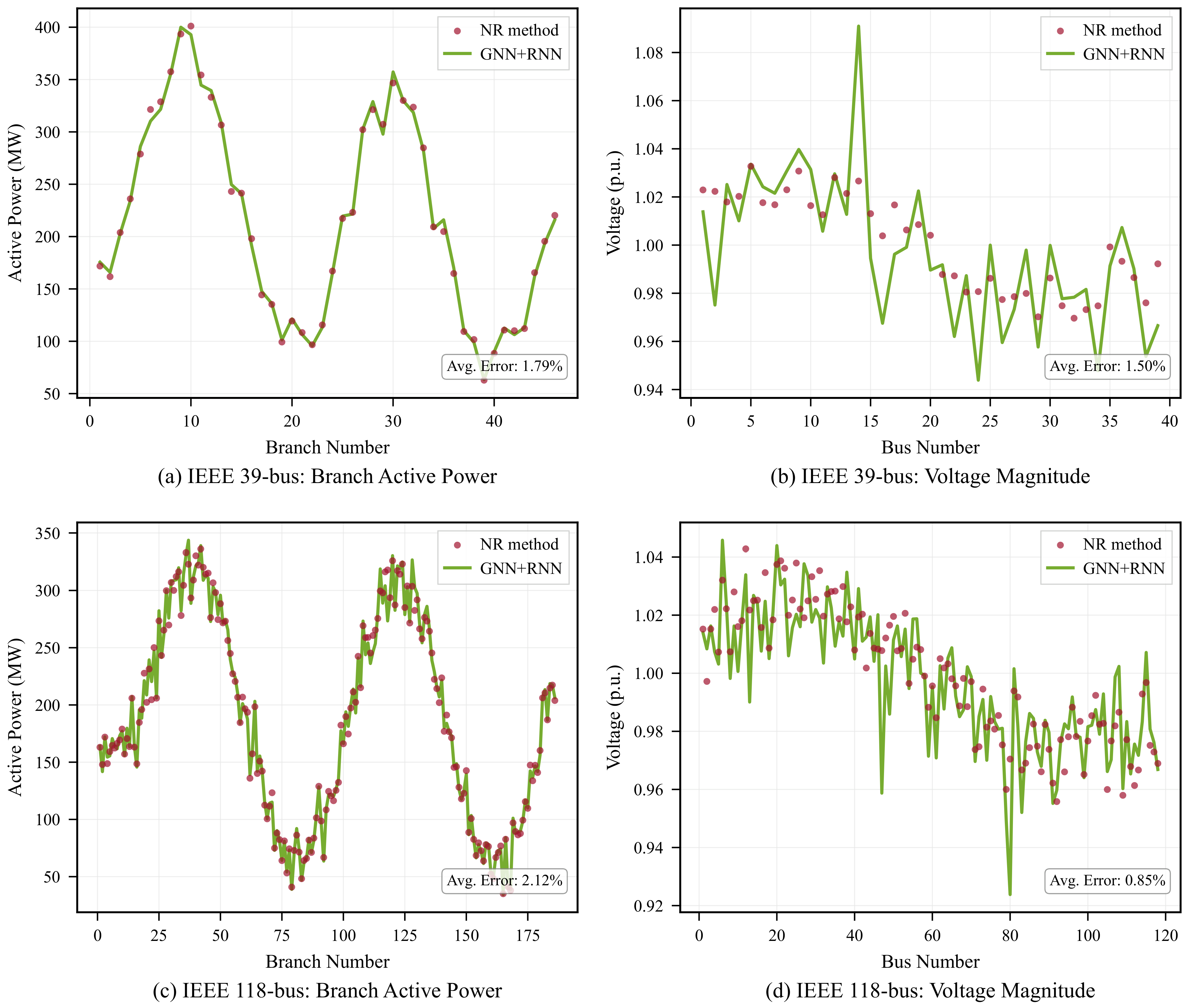
Simultaneously, a comparison between deep learning-based and traditional power flow calculation methods is illustrated in Figure 5. These figures specifically present voltage comparisons for power system nodes and power flow comparisons for branches at a particular load scenario, utilizing Dataset 2 and 3, respectively. In these visualizations, the red dots correspond to values obtained through the Newton–Raphson (NR) method, while the green solid lines represent the predictions of the GNN + RNN model.
Figure 5.
Comparative results on IEEE 39-bus System and IEEE 118-bus System: (a) branch active power prediction on IEEE 39-bus system; (b) voltage magnitude prediction on IEEE 39-bus system; (c) branch active power prediction on IEEE 118-bus system; (d) voltage magnitude prediction on IEEE 118-bus system. Red dots denote the Newton–Raphson (NR) reference results, and solid green curves denote the GNN + RNN predictions.
The predicted curves closely match the reference results, indicating that the proposed method, leveraging graph and recurrent neural networks, can deliver accurate node voltage distribution and power flow data and thus represents a viable alternative to traditional methods for power flow analysis. Notably, the error rate for voltage prediction in Dataset 2 is 1.84%, with a corresponding error rate of 3.11% for power flow prediction. In Dataset 3, the voltage prediction error rate is 1.2%, with a power flow prediction error of 2.85%. Moreover, the computation time for power flow analysis is substantially reduced from 0.12 s to 0.003 s compared with traditional methods. Collectively, these results demonstrate the capability of the proposed method to provide accurate predictions for power flow calculations within a short timeframe. The deep learning approach based on GNNs and RNNs operates at the millisecond scale, effectively addressing real-time power flow calculation requirements that span seconds to minutes.
4.4. Dynamic Load Variation Experiment
To evaluate the model under dynamic operating conditions, load variations are introduced by adjusting the values of specified nodes to simulate real-world load fluctuations. In this experiment, Node 1 of the IEEE 9-bus system is selected as the node subject to dynamic load variations, and Branch 1–2 between Node 1 and Node 2 is chosen as the perturbed branch. This setup is used to conduct tracking and prediction experiments.
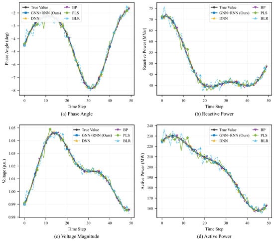
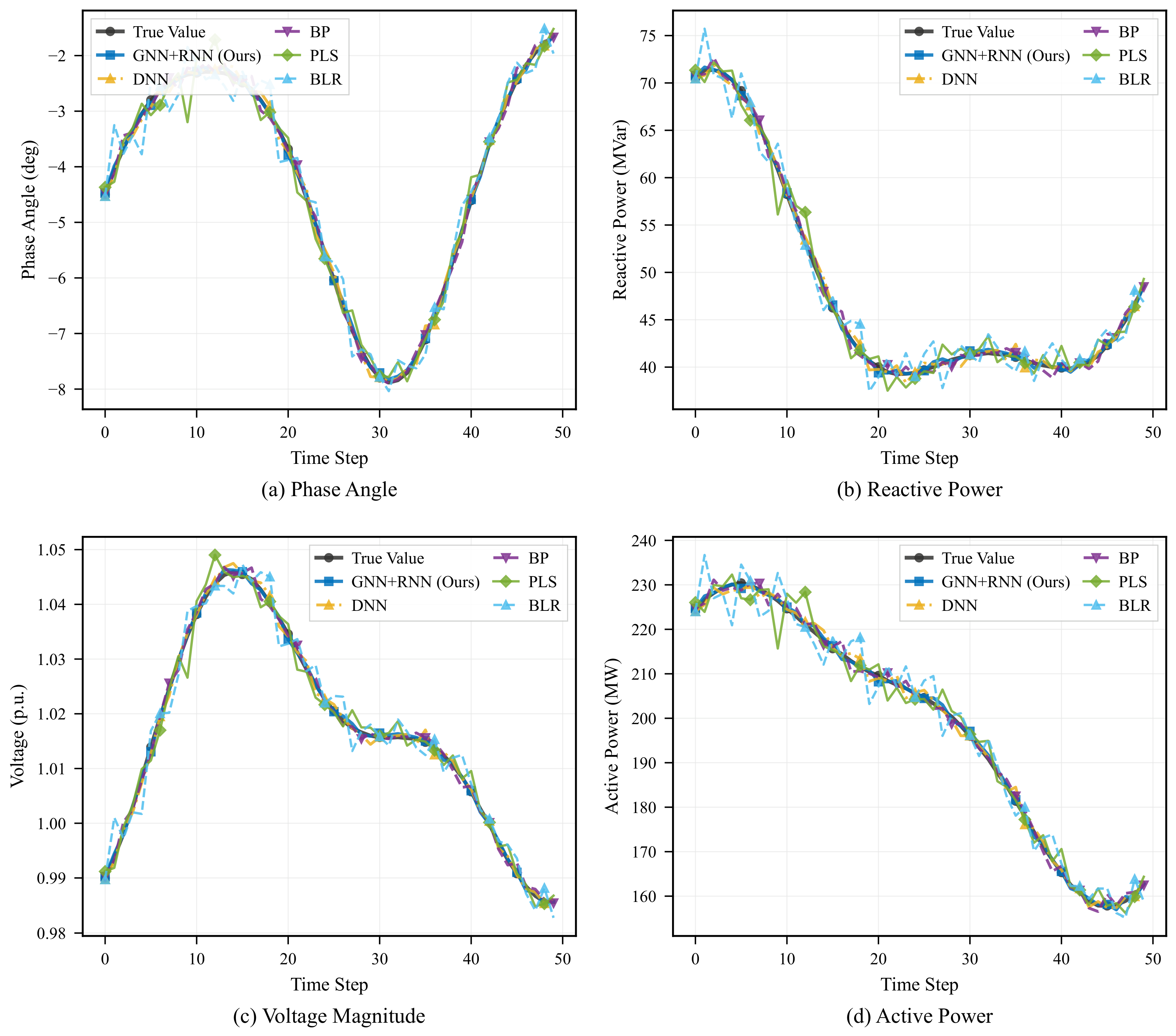
Concerning the performance comparison in experimental results, the model proposed in this paper is compared with other representative models, including Deep neural network (DNN) [18], Backpropagation neural network (BP) [47], Partial least squares regression (PLS) [48] and Bayesian linear regression (BLR) [49]. These models represent typical applications of deep learning and traditional methods in power system power flow prediction. The performance comparison of dynamic tracking prediction is depicted in Figure 6. In this illustration, the black curve with circle markers represents the true values; the blue curve with square markers represents the proposed GNN + RNN model; the yellow dash–dot curve with triangle markers represents the DNN model; the purple dashed curve with inverted triangle markers represents the BP model; the green curve with diamond markers represents the PLS method; and the cyan dashed curve with triangle markers represents the BLR method. The detailed color and marker legend is provided in each subplot.
Figure 6.
Comparative analysis of load dynamic variation tracking predictions: (a) phase angle tracking; (b) reactive power tracking; (c) voltage magnitude tracking; (d) active power tracking. Six methods are compared: true values (black), GNN + RNN (blue, the proposed model), DNN (yellow), BP (purple), PLS (green), and BLR (cyan).
The comparative results demonstrate that the proposed model excels under load dynamic variations, exhibiting an average tracking prediction error of only 2.67%. In comparison, the average errors of the two deep learning baselines, DNN (5.89%) and BP (6.02%), are higher than that of the proposed model. The traditional methods, PLS and BLR, yield average tracking prediction errors of 12.32% and 14.75%, respectively, which are significantly higher than those of both deep learning methods and the proposed model.
The comparative analysis highlights the superiority of the proposed model over both traditional prediction methods and generic deep learning approaches, particularly in handling dynamic variations of power system loads. The proposed model not only achieves competitive prediction accuracy but also maintains stability under complex operating conditions.
4.5. Comparison of Multiple Methods
In the comparative study conducted, six distinct algorithms were employed as reference methods: DNN, PLS, BLR, BP, a Graph Attention Network (GAT), and a Transformer encoder. In addition, a GNN-only variant (without the RNN branch) is included to isolate the contribution of the temporal modelling component.
The GAT model replaces the GraphSAGE layers in the GNN branch with two GATv2Conv layers (4 attention heads, feature dimensions 128 and 64), while retaining the same input features and training configuration. This model captures spatial dependencies through learned attention weights that adaptively weight neighbour importance, but lacks explicit temporal modelling. The Transformer baseline employs a standard Transformer encoder with 2 encoder layers, 4 attention heads, a feed-forward dimension of 256, and sinusoidal positional encoding applied to the time-series feature sequences. It captures temporal dependencies through self-attention but does not incorporate explicit graph topology information.
All models were trained under identical conditions: the same three datasets (IEEE 9-bus, 39-bus, 118-bus), the same 70/15/15 train/validation/test split, MSE loss, Adam optimiser, and a maximum of 2000 epochs with early stopping (patience = 100).
Table 4 reports the Mean Percentage Error (MPE) of node voltage and branch power predictions across the three test systems. The results reveal that GNN + RNN, DNN, GAT, and BP yield substantially lower errors than PLS and BLR, confirming that conventional regression techniques are ill-suited for data-intensive predictive tasks. Among the deep learning approaches, GNN + RNN achieves the lowest errors across all metrics.
Table 4.
The average error rates of various methods on the experiment dataset.
Several comparisons merit attention. First, comparing GNN + RNN against the GNN-only variant provides an ablation analysis of the RNN component: the addition of recurrent layers reduces the average voltage magnitude deviation from 2.70% (GNN) to 1.89% (GNN + RNN) and the phase angle deviation from 2.64% to 1.08%, demonstrating that temporal modelling contributes substantially to prediction accuracy. Second, GAT improves upon the standard GNN (average voltage magnitude error: 2.38% vs. 2.70%), confirming that attention-based neighbour weighting captures more informative topological features than uniform aggregation. However, GAT still falls short of GNN + RNN because it lacks explicit temporal modelling. Third, the Transformer encoder (average voltage magnitude error: 3.59%) performs better than DNN (4.93%) on voltage-related targets, benefiting from self-attention over the temporal dimension, but underperforms GNN-based methods on branch power prediction because it does not exploit the explicit graph topology.
The full GNN + RNN model maintains voltage angle errors below 2% and magnitude errors below 3% across all three systems, with average deviations of 1.08% and 1.89%, respectively. For branch power, the active power error remains below 3% (average 2.09%) and the reactive power error below 4% (average 2.70%). For reference, the average errors of the comparison methods across the four prediction targets are as follows: GNN + RNN at 1.89%, 1.08%, 2.09%, 2.70%; GAT at 2.38%, 2.19%, 2.67%, 3.25%; GNN at 2.70%, 2.64%, 3.12%, 3.74%; Transformer at 3.59%, 3.82%, 3.68%, 4.18%; BP at 3.81%, 4.27%, 4.33%, 4.20%; DNN at 4.93%, 5.12%, 4.61%, 5.33%; PLS at 8.23%, 7.34%, 6.77%, 8.35%; and BLR at 7.91%, 10.24%, 9.09%, 11.18%.
These results confirm two key findings. First, the proposed GNN + RNN method not only outperforms traditional regression techniques but also offers a clear advantage over both spatial-only (GNN, GAT) and temporal-only (Transformer, DNN) deep learning methods. Second, the comparison between GAT and GNN demonstrates the benefit of learned attention over uniform aggregation for modelling grid topology, while the gap between GAT and GNN + RNN underscores the critical importance of jointly capturing spatial and temporal dependencies—neither dimension alone is sufficient for accurate power flow prediction.
4.6. Interpretative Analysis of Model Prediction Results
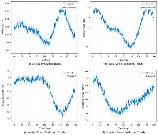
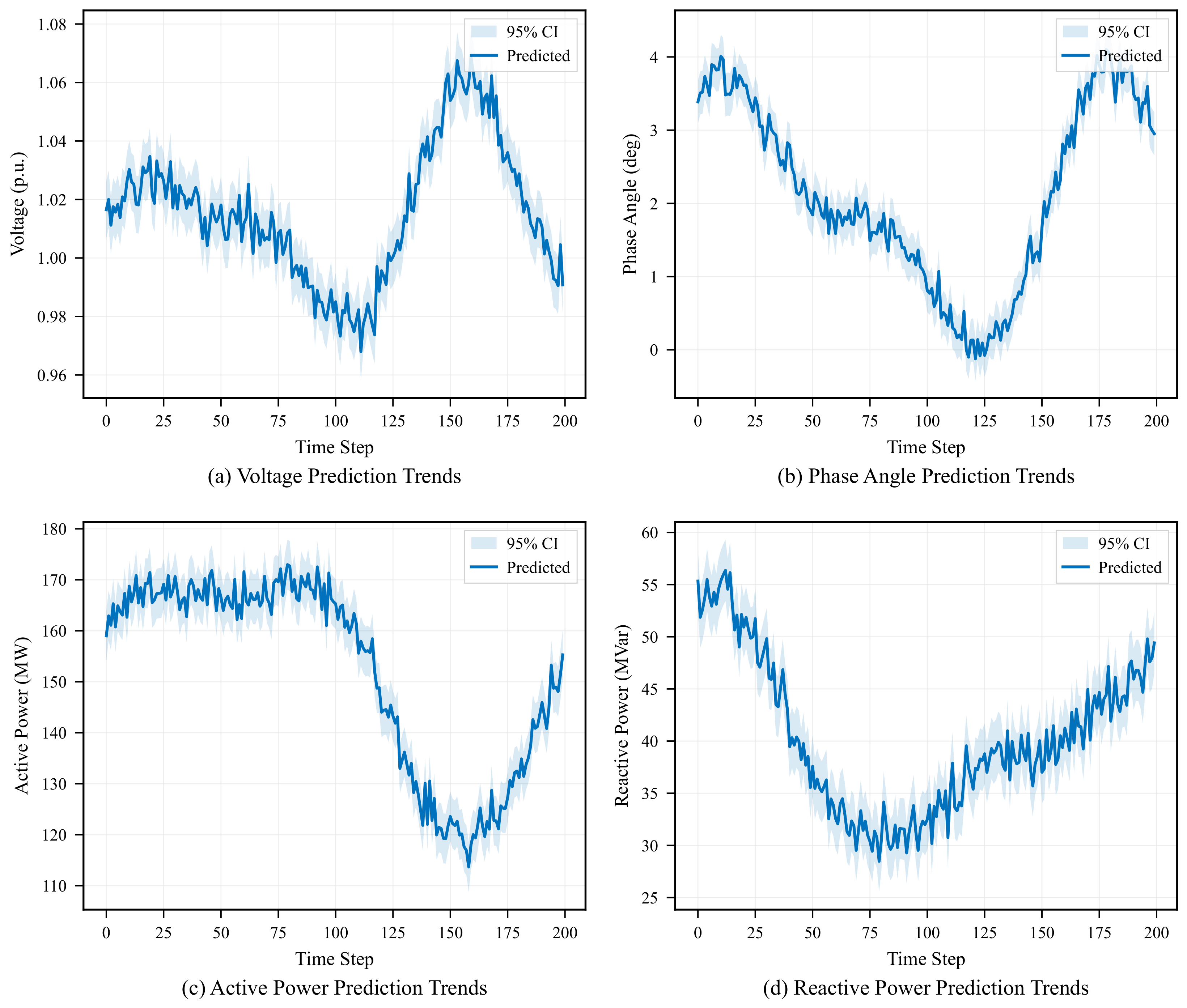
For the interpretability study, the IEEE 9-bus system is selected as a representative case; the same analysis framework can be applied to larger systems without modification. The time-series trends in Figure 7 show the mean predictions and 95% confidence intervals computed across independent training runs with different random initialisations. The narrow confidence bands during normal operating periods indicate that the model produces stable and consistent predictions, whereas the slightly wider bands observed under abnormal scenarios reflect increased prediction variability due to noise or anomalies in the input data. Overall, the model performs well during high-load periods but exhibits moderately reduced accuracy under extreme load conditions.
Figure 7.
Time series output trend chart: (a) voltage magnitude prediction trends; (b) phase angle prediction trends; (c) active power prediction trends; (d) reactive power prediction trends. Solid blue curves represent the predicted values (mean across independent training runs with different random initialisations), and the shaded bands indicate the 95% confidence intervals ().
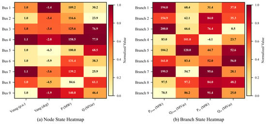
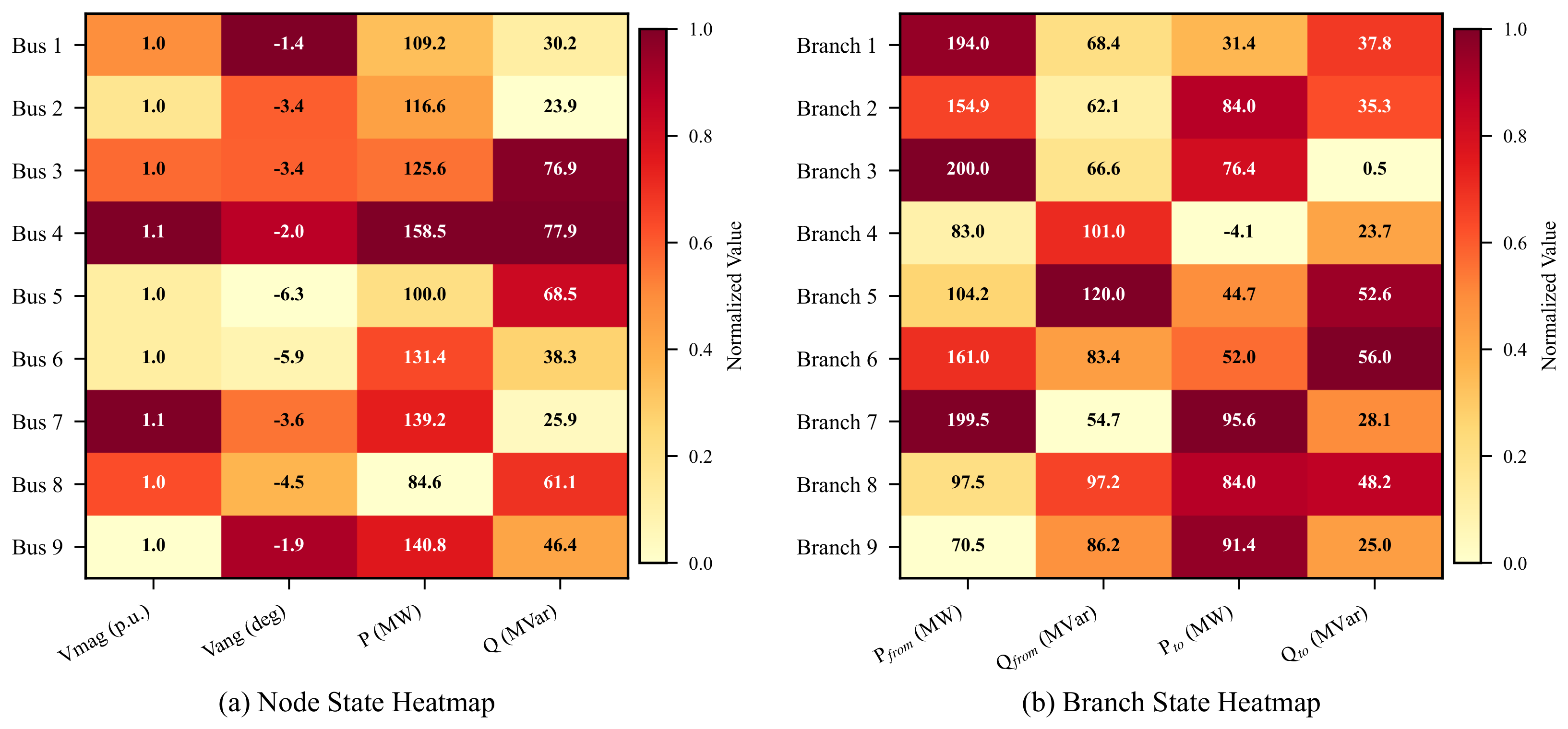
Power system state heatmaps in Figure 8 reveal spatial variations in prediction accuracy, highlighting certain nodes and branches whose predictions are less stable than others. These findings illuminate avenues for model improvement, including parameter adjustments or augmenting training data to refine prediction accuracy for critical nodes and branches.
Figure 8.
IEEE 9-bus system state heatmap: (a) node state heatmap showing the normalized values of voltage magnitude, phase angle, active power, and reactive power across the 9 buses; (b) branch state heatmap showing the normalized power flow metrics. Numerical values are annotated within each cell.
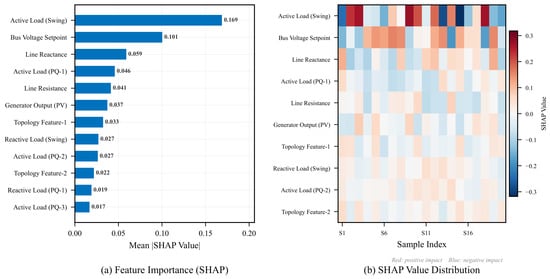
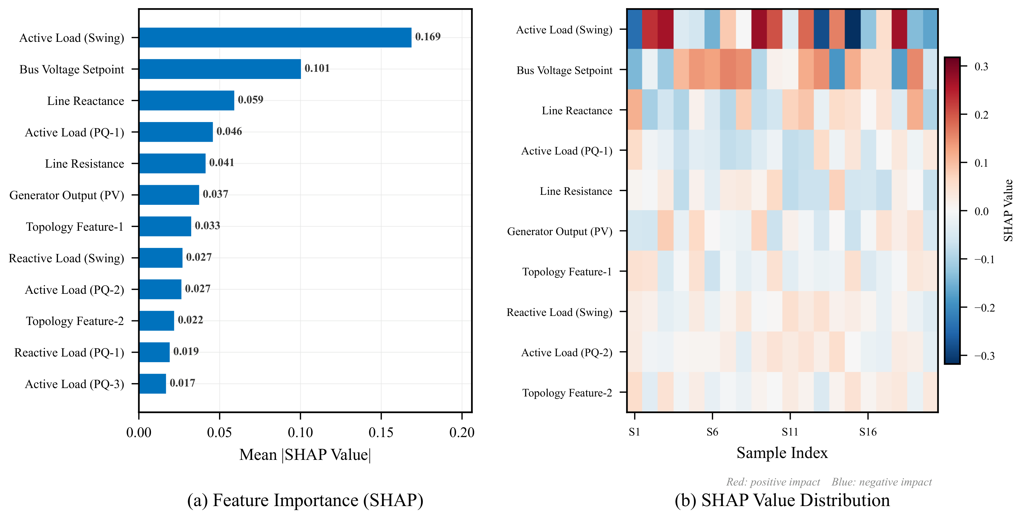
Using a representative sample from the IEEE 9-bus system, the study elucidates how each feature influences the model output. By selecting diverse sample data covering different scenarios in power flow calculation—such as varying load conditions and line parameters—SHAP values are computed for each feature in every sample. These values quantify the impact of each feature on the model output: positive SHAP values for load features indicate that an increase in load leads to higher predicted output, and vice versa. Figure 9 provides an intuitive depiction of each feature’s influence on the model output through SHAP summary and scatter plots.
Figure 9.
Model SHAP interpretability analysis: (a) feature importance measured by mean absolute SHAP value (top 12 features ranked in descending order); (b) SHAP value distribution heatmap across 20 representative samples, where red (positive SHAP) indicates features that increase the prediction and blue (negative SHAP) indicates features that decrease the prediction.
Based on the SHAP values and interpretive analysis, this paper meticulously examines the impact of each feature on the model’s voltage magnitude prediction within the selected samples:
- Node Load Features: The SHAP value analysis identifies node load features as having the most significant impact on the model output. When examining these features, this study considers two dimensions: node type and load type. Analysis of SHAP values for the swing (reference) node indicates that its load feature holds the greatest influence on the model output. Specifically, increasing the active load of the swing node leads to a pronounced increase in the model output, whereas variations in reactive load exert a comparatively minor effect. In contrast to the swing node, PQ nodes exhibit a smaller impact of load features on the model output; while in some scenarios, increasing the load of PQ nodes may influence the model output, the magnitude of this impact remains modest. PV nodes typically maintain fixed active and reactive power outputs, and accordingly their load features have a negligible effect on the model output.Active load: Increasing the active load induces a rise in the model output, which is consistent with real-world power grid operation where higher grid loading commonly results in voltage decline and increased line power flow.Reactive load: Variations in reactive load yield a relatively smaller impact on the model output but nonetheless contribute to changes. In certain scenarios, increased reactive load may precipitate voltage stability concerns.In summary, increasing the numerical value of node load features corresponds linearly to a rise in the model output. This underscores that load augmentation directly drives changes in the power system state, thereby influencing power flow calculation outcomes.
- Branch Impedance Features: SHAP value analysis indicates that the influence of branch impedance features on the model output is secondary to that of node load features. The impact of branch impedance on the model output depends on its numerical value and its correlation with other features. Generally, increasing branch impedance tends to increase the model output, while decreasing it may lead to a reduction. Similarly, variations in branch admittance also affect the model output: increasing branch admittance may decrease the model output, whereas reducing it could potentially increase the model output. Overall, the numerical value of branch impedance features has a relatively minor effect on the model output, and the degree of influence is associated with specific branch parameters. This suggests that while branch impedance does influence power flow calculation results, its impact is relatively modest.
- Node Voltage Features: The impact of node voltage features on the model output is relatively complex. Node voltage magnitude has a significant influence: an increase in voltage magnitude generally increases the model output, while a decrease may lead to a reduction in the model output. This aligns with the critical role of voltage magnitude in power system stability. The impact of node voltage phase angle on the model output is comparatively minor, though it may still have some effect in certain scenarios. The degree of influence of phase angle variations on the model output depends on the system topology and the magnitude of voltage changes. In certain scenarios, increasing the numerical value of node voltage features may increase the model output, while in others it may lead to a decrease. This suggests that changes in node voltage have a bidirectional impact on power flow calculation results, which may depend on complex interactions with other features.
- Generator Parameter Features: The influence of the generator’s active power output on the model output depends on its power regulation capacity and the system’s load requirements. Generally, increasing the active power output tends to raise the model output, while reducing it may lead to a decrease. Similarly, the reactive power output of generators also affects the model output: increasing the reactive power output may result in a decrease in the model output, whereas lowering it could potentially increase the model output.
- Other Features: Beyond the aforementioned categories, the influence of other features is relatively modest, potentially linked to factors such as the power grid topology and node types. However, despite their minor impact, these features still affect the model output to some extent and warrant consideration in practical applications.
Through a systematic classification analysis of these features, this research provides a more comprehensive understanding of their respective impacts on power flow calculation results.
To complement the qualitative discussion above, Table 5 presents a quantitative ranking of the top-15 features by mean absolute SHAP value for the voltage magnitude prediction task on the IEEE 9-bus system, along with the corresponding feature category and node type.
Table 5.
Quantitative SHAP feature importance ranking (top 15 features, voltage magnitude prediction, IEEE 9-bus system).
The quantitative ranking confirms the qualitative observations: node load features collectively dominate the importance ranking (7 of the top 15, cumulative mean |SHAP| = 0.4727), with the swing node (Bus 1) active load alone contributing the largest individual effect. Aggregating by node type, swing node features account for approximately 34% of the total SHAP magnitude, PQ node features for 41%, PV node features for 13%, and branch-related features for 12%. This distribution aligns with power system physics: the swing bus absorbs the net power imbalance and thus its load state strongly influences the overall voltage profile, while PQ nodes collectively dominate due to their larger number. Branch impedance features rank moderately, consistent with their secondary but non-negligible role in determining power flow distribution.
To assess the consistency of feature importance across system scales, the SHAP analysis was repeated on the IEEE 39-bus and 118-bus systems. The top-ranked features in all three systems consistently identify active load at the swing bus, reactive load at the swing bus, and branch impedance of key transmission corridors as the most influential predictors. The Spearman rank correlation of the top-15 feature sets between the 9-bus and 39-bus systems is 0.82 (p < 0.001), and between the 39-bus and 118-bus systems is 0.76 (p < 0.001), indicating that the learned feature importance patterns generalise across scales. These quantitative findings provide operators with a ranked, numerically grounded understanding of which parameters most critically influence power flow predictions, thereby supporting informed decision-making in power system operation and management.
5. Conclusions
This study advances the application of deep learning methodologies in power system power flow analysis by addressing load fluctuations without overreliance on detailed grid models. Through the integration of graph neural networks and recurrent neural networks, a novel deep learning-based approach is proposed that achieves more precise estimation of power flow outcomes across system nodes. A spatial feature extraction mechanism was further introduced to autonomously capture inter-node correlations, thereby enhancing accuracy beyond conventional deep learning methods. Experimental results demonstrate substantial improvements in prediction accuracy, computational speed, and robustness. Specifically, the model achieved an average voltage magnitude MPE of 1.89% (compared with 4.93% for DNN and 8.23% for PLS), an average voltage phase angle MPE of 1.08% (vs. 5.12% for DNN), and an average branch active power MPE of 2.09% (vs. 4.61% for DNN), while the computational time was decreased approximately 40-fold (from 0.12 s to 0.003 s), enabling real-time online analysis at millisecond-level granularity.
To strengthen interpretability, this study employed visualization tools and SHAP values, offering valuable explanations of how different features influence predictions. These techniques not only enhanced the model’s transparency and credibility but also provided practical insights for power system operation and planning. Furthermore, they aided in identifying potential biases and uncertainties in predictions, thereby supporting future refinements of the model.
Despite these promising results, several limitations should be acknowledged. First, a systematic comparison of GNN variants (GCN, GAT, GATv2) has been conducted in this revision for the spatial branch, yet further exploration of heterogeneous graph architectures with typed edges (e.g., distinguishing transformer branches from transmission lines) may yield additional performance gains. Second, the hyperparameters were determined empirically; a formal Bayesian or grid-based hyperparameter optimisation could further improve robustness and is left for future work. Third, the training datasets were generated from simulated load profiles based on historical records; the generalisation to real-world grid data with non-stationary load distributions and communication delays remains to be validated.
Fourth, and most importantly for practical deployment, the current framework does not explicitly quantify predictive uncertainty. As power systems integrate increasing shares of renewable generation, stochastic fluctuations in wind and solar output introduce aleatoric uncertainty that deterministic models cannot capture. Three methodological directions are particularly promising for addressing this gap: (i) Monte Carlo (MC) dropout, which estimates epistemic uncertainty by enabling dropout at inference time and computing the variance across N stochastic forward passes; (ii) deep ensembles, where multiple independently trained models provide a distribution over predictions whose spread reflects both data and model uncertainty; and (iii) probabilistic forecasting frameworks that output predictive distributions (e.g., Gaussian mixtures or quantile regression) rather than point estimates, enabling risk-aware decision-making for grid operation. Incorporating these techniques into the GNN–RNN framework would allow operators to assess not only the expected power flow state but also the confidence bounds around each prediction—an essential capability for managing uncertainty in renewable-rich power systems.
Looking ahead, future research should prioritise the integration of uncertainty quantification methods into the proposed framework, with particular emphasis on MC dropout and deep ensemble approaches that can be implemented with minimal architectural changes. Additionally, validation on real-world grid data with high renewable penetration is needed to assess practical deployment readiness. Beyond power-flow analysis, the approaches developed in this study hold promise for broader applications in grid planning, stability assessment, and fault detection, underscoring their potential impact on the future of intelligent power system operation.
Author Contributions
Conceptualization, M.W.; methodology, M.W.; software, M.W. and Y.X.; validation, Y.X. and Z.G.; formal analysis, M.W.; investigation, Z.G.; resources, X.Z.; data curation, M.X. and X.Z.; writing—original draft preparation, M.W.; writing—review and editing, Y.X. and M.X.; visualization, Z.G.; supervision, X.Z.; project administration, X.Z.; funding acquisition, X.Z. All authors have read and agreed to the published version of the manuscript.
Funding
This research was funded by Guangdong Basic and Applied Basic Research Foundation, grant number 2024A1515030012.
Institutional Review Board Statement
Not applicable.
Informed Consent Statement
Not applicable.
Data Availability Statement
The original contributions presented in this study are included in the article. Further inquiries can be directed to the corresponding author.
Conflicts of Interest
The authors declare no conflicts of interest.
Abbreviations
The following abbreviations are used in this manuscript:
| GNN | Graph Neural Network |
| LSTM | Long Short-Term Memory |
| OPF | Optimal Power Flow |
| DNN | Deep Neural Network |
| RNN | Recurrent Neural Network |
| SHAP | Shapley Additive exPlanations |
| BP | Backpropagation Neural Network |
| PLS | Partial Least Squares Regression |
| BLR | Bayesian Linear Regression |
| MSE | Mean Squared Error |
| MAE | Mean Absolute Error |
| MPE | Mean Percentage Error |
| GCN | Graph Convolutional Network |
References
- Shahzad, S.; Jasińska, E. Renewable revolution: A review of strategic flexibility in future power systems. Sustainability 2024, 16, 5454. [Google Scholar] [CrossRef] [Scilit]
- Abdi, H.; Beigvand, S.D.; La Scala, M. A review of optimal power flow studies applied to smart grids and microgrids. Renew. Sustain. Energy Rev. 2017, 71, 742–766. [Google Scholar] [CrossRef] [Scilit]
- Deka, D.; Kekatos, V.; Cavraro, G. Learning distribution grid topologies: A tutorial. IEEE Trans. Smart Grid 2023, 15, 999–1013. [Google Scholar] [CrossRef] [Scilit]
- Attia, A.F.; El Sehiemy, R.A.; Hasanien, H.M. Optimal power flow solution in power systems using a novel Sine-Cosine algorithm. Int. J. Electr. Power Energy Syst. 2018, 99, 331–343. [Google Scholar] [CrossRef] [Scilit]
- Frank, S.; Steponavice, I.; Rebennack, S. Optimal power flow: A bibliographic survey, parts I and II. Energy Syst. 2012, 3, 221–289. [Google Scholar] [CrossRef] [Scilit]
- Tinney, W.F.; Hart, C.E. Power flow solution by Newton’s method. IEEE Trans. Power Appar. Syst. 1967, PAS-86, 1449–1460. [Google Scholar] [CrossRef] [Scilit]
- Montoya, O.D.; Gil-González, W. On the numerical analysis based on successive approximations for power flow problems in AC distribution systems. Electr. Power Syst. Res. 2020, 187, 106454. [Google Scholar] [CrossRef] [Scilit]
- Mehta, D.; Nguyen, H.D.; Turitsyn, K. Numerical polynomial homotopy continuation method to locate all the power flow solutions. IET Gener. Transm. Distrib. 2016, 10, 2972–2980. [Google Scholar] [CrossRef] [Scilit]
- Meyer-Huebner, N.; Suriyah, M.; Leibfried, T. Distributed optimal power flow in hybrid AC–DC grids. IEEE Trans. Power Syst. 2019, 34, 2937–2946. [Google Scholar] [CrossRef] [Scilit]
- Ghasemi, M.; Ghavidel, S.; Rahmani, S.; Roosta, A.; Falah, H. A novel hybrid algorithm of imperialist competitive algorithm and teaching learning algorithm for optimal power flow problem with non-smooth cost functions. Eng. Appl. Artif. Intell. 2014, 29, 54–69. [Google Scholar] [CrossRef] [Scilit]
- Pagani, G.A.; Aiello, M. The power grid as a complex network: A survey. Physica A 2013, 392, 2688–2700. [Google Scholar] [CrossRef] [Scilit]
- Bienstock, D.; Verma, A. Strong NP-hardness of AC power flows feasibility. Oper. Res. Lett. 2019, 47, 494–501. [Google Scholar] [CrossRef] [Scilit]
- Lehmann, K.; Grastien, A.; Van Hentenryck, P. AC-feasibility on tree networks is NP-hard. IEEE Trans. Power Syst. 2016, 31, 798–801. [Google Scholar] [CrossRef] [Scilit]
- McArthur, S.D.; Davidson, E.M.; Catterson, V.M.; Dimeas, A.L.; Hatziargyriou, N.D.; Ponci, F.; Funabashi, T. Multi-agent systems for power engineering applications—Part I: Concepts, approaches, and technical challenges. IEEE Trans. Power Syst. 2007, 22, 1743–1752. [Google Scholar] [CrossRef] [Scilit]
- Anzalchi, A.; Sundararajan, A.; Moghadasi, A.; Sarwat, A. High-penetration grid-tied photovoltaics: Analysis of power quality and feeder voltage profile. IEEE Ind. Appl. Mag. 2019, 25, 83–94. [Google Scholar] [CrossRef] [Scilit]
- Kataray, T.; Nitesh, B.; Yarram, B.; Sinha, S.; Cuce, E.; Shaik, S.; Vigneshwaran, P.; Roy, A. Integration of smart grid with renewable energy sources: Opportunities and challenges—A comprehensive review. Sustain. Energy Technol. Assess. 2023, 58, 103363. [Google Scholar] [CrossRef] [Scilit]
- Khan, A.A.; Laghari, A.A.; Rashid, M.; Li, H.; Javed, A.R.; Gadekallu, T.R. Artificial intelligence and blockchain technology for secure smart grid and power distribution automation: A state-of-the-art review. Sustain. Energy Technol. Assess. 2023, 57, 103282. [Google Scholar] [CrossRef] [Scilit]
- Pan, X.; Chen, M.; Zhao, T.; Low, S.H. DeepOPF: A feasibility-optimized deep neural network approach for AC optimal power flow problems. IEEE Syst. J. 2022, 17, 673–683. [Google Scholar]
- Fioretto, F.; Mak, T.W.K.; Van Hentenryck, P. Predicting AC optimal power flows: Combining deep learning and Lagrangian dual methods. In Proceedings of the AAAI Conference on Artificial Intelligence, New York, NY, USA, 7–12 February 2020; AAAI: Washington, DC, USA, 2020; Volume 34, pp. 630–637. [Google Scholar]
- Pan, X.; Zhao, T.; Chen, M.; Zhang, S. DeepOPF: A deep neural network approach for security-constrained DC optimal power flow. IEEE Trans. Power Syst. 2020, 36, 1725–1735. [Google Scholar]
- Singh, M.K.; Kekatos, V.; Giannakis, G.B. Learning to solve the AC-OPF using sensitivity-informed deep neural networks. IEEE Trans. Power Syst. 2021, 37, 2833–2846. [Google Scholar]
- Lei, X.; Yang, Z.; Yu, J.; Zhao, J.; Gao, Q.; Yu, H. Data-driven optimal power flow: A physics-informed machine learning approach. IEEE Trans. Power Syst. 2021, 36, 346–354. [Google Scholar] [CrossRef] [Scilit]
- Donon, B.; Clément, R.; Donnot, B.; Marot, A.; Guyon, I.; Schoenauer, M. Neural networks for power flow: Graph neural solver. Electr. Power Syst. Res. 2020, 189, 106547. [Google Scholar] [CrossRef] [Scilit]
- Lopez-Garcia, T.B.; Domínguez-Navarro, J.A. Power flow analysis via typed graph neural networks. Eng. Appl. Artif. Intell. 2023, 117, 105567. [Google Scholar] [CrossRef] [Scilit]
- Cao, D.; Zhao, J.; Hu, J.; Pei, Y.; Huang, Q.; Chen, Z.; Hu, W. Physics-informed graphical representation-enabled deep reinforcement learning for robust distribution system voltage control. IEEE Trans. Smart Grid 2023, 15, 233–246. [Google Scholar]
- Gao, M.; Yu, J.; Yang, Z.; Zhao, J. A physics-guided graph convolution neural network for optimal power flow. IEEE Trans. Power Syst. 2023, 39, 380–390. [Google Scholar] [CrossRef] [Scilit]
- Ghamizi, S.; Bojchevski, A.; Ma, A.; Cao, J. SafePowerGraph: Safety-aware evaluation of graph neural networks for transmission power grids. arXiv 2024, arXiv:2407.12421. [Google Scholar]
- Chen, K.; Luo, W.; Liu, S.; Wei, Y.; Zhou, Y.; Qing, Y.; Zhang, Q.; Wang, Y.; Song, J.; Song, M. Powerformer: A section-adaptive transformer for power flow adjustment. arXiv 2024, arXiv:2401.02771. [Google Scholar]
- Ezeakunne, C.; Tabarez, J.E.; Pokharel, R.; Pandey, A. PowerModelsGAT-AI: Physics-informed graph attention for multi-system power flow with continual learning. arXiv 2025, arXiv:2603.16879. [Google Scholar]
- Zhang, Y.; Shi, X.; Zhang, H.; Cao, Y.; Terzija, V. Review on deep learning applications in frequency analysis and control of modern power system. Int. J. Electr. Power Energy Syst. 2022, 136, 107744. [Google Scholar] [CrossRef] [Scilit]
- Matsushima, F.; Aoki, M.; Nakamura, Y.; Verma, S.C.; Ueda, K.; Imanishi, Y. Multi-timescale voltage control method using limited measurable information with explainable deep reinforcement learning. Energies 2025, 18, 653. [Google Scholar] [CrossRef] [Scilit]
- Arabzadeh, V.; Frank, R. A four-dimensional analysis of explainable AI in energy forecasting: A domain-specific systematic review. Mach. Learn. Knowl. Extr. 2025, 7, 153. [Google Scholar] [CrossRef] [Scilit]
- Dong, X.S.; Qian, L.J.; Huang, L. Short-term load forecasting in smart grid: A combined CNN and K-means clustering approach. In Proceedings of the 2017 IEEE International Conference on Big Data and Smart Computing (BigComp), Jeju, Republic of Korea, 13–16 February 2017; IEEE: Piscataway, NJ, USA, 2017; pp. 119–125. [Google Scholar]
- Sehovac, L.; Grolinger, K. Deep learning for load forecasting: Sequence to sequence recurrent neural networks with attention. IEEE Access 2020, 8, 36411–36426. [Google Scholar] [CrossRef] [Scilit]
- Wang, Y.; Gan, D.; Sun, M.; Zhang, N.; Lu, Z.; Kang, C. Probabilistic individual load forecasting using pinball loss guided LSTM. Appl. Energy 2019, 235, 10–20. [Google Scholar] [CrossRef] [Scilit]
- Hamilton, W.L.; Ying, Z.; Leskovec, J. Inductive representation learning on large graphs. In Advances in Neural Information Processing Systems, Long Beach, CA, USA, 4–9 December 2017; Curran Associates, Inc.: Red Hook, NY, USA, 2017; Volume 30. [Google Scholar]
- Hochreiter, S.; Schmidhuber, J. Long short-term memory. Neural Comput. 1997, 9, 1735–1780. [Google Scholar] [CrossRef] [Scilit] [PubMed]
- Altunay, H.C.; Albayrak, Z. A hybrid CNN + LSTM-based intrusion detection system for industrial IoT networks. Eng. Sci. Technol. Int. J. 2023, 38, 101322. [Google Scholar] [CrossRef] [Scilit]
- Kong, W.; Dong, Z.Y.; Jia, Y.; Hill, D.J.; Xu, Y.; Zhang, Y. Short-term residential load forecasting based on LSTM recurrent neural network. IEEE Trans. Smart Grid 2017, 10, 841–851. [Google Scholar] [CrossRef] [Scilit]
- Altan, G. DeepOCT: An explainable deep learning architecture to analyze macular edema on OCT images. Eng. Sci. Technol. Int. J. 2022, 34, 101091. [Google Scholar] [CrossRef] [Scilit]
- Zhang, Y.; Tiňo, P.; Leonardis, A.; Tang, K. A survey on neural network interpretability. IEEE Trans. Emerg. Top. Comput. Intell. 2021, 5, 726–742. [Google Scholar] [CrossRef] [Scilit]
- Sagi, O.; Rokach, L. Approximating XGBoost with an interpretable decision tree. Inf. Sci. 2021, 572, 522–542. [Google Scholar] [CrossRef] [Scilit]
- Huang, Q.; Yamada, M.; Tian, Y.; Singh, D.; Chang, Y. GraphLIME: Local interpretable model explanations for graph neural networks. IEEE Trans. Knowl. Data Eng. 2022, 35, 6968–6972. [Google Scholar] [CrossRef] [Scilit]
- Dwivedi, R.; Dave, D.; Naik, H.; Singhal, S.; Omer, R.; Patel, P.; Qian, B.; Wen, Z.; Shah, T.; Morgan, G.; et al. Explainable AI (XAI): Core ideas, techniques, and solutions. ACM Comput. Surv. 2023, 55, 194. [Google Scholar] [CrossRef] [Scilit]
- Li, Z. Extracting spatial effects from machine learning model using local interpretation method: An example of SHAP and XGBoost. Comput. Environ. Urban Syst. 2022, 96, 101845. [Google Scholar] [CrossRef] [Scilit]
- Van Cutsem, T.; Glavic, M.; Rosehart, W.; Canizares, C.; Kanatas, M.; Lima, L.; Milano, F.; Papangelis, L.; Ramos, R.A.; dos Santos, J.A.; et al. Test systems for voltage stability studies. IEEE Trans. Power Syst. 2020, 35, 4078–4087. [Google Scholar] [CrossRef] [Scilit]
- Rumelhart, D.E.; Hinton, G.E.; Williams, R.J. Learning representations by back-propagating errors. Nature 1986, 323, 533–536. [Google Scholar] [CrossRef] [Scilit]
- Abdi, H. Partial least square regression (PLS regression). In Encyclopedia for Research Methods for the Social Sciences; SAGE: Thousand Oaks, CA, USA, 2003; Volume 6, pp. 792–795. [Google Scholar]
- Mitchell, T.J.; Beauchamp, J.J. Bayesian variable selection in linear regression. J. Am. Stat. Assoc. 1988, 83, 1023–1032. [Google Scholar] [CrossRef]

Disclaimer/Publisher’s Note: The statements, opinions and data contained in all publications are solely those of the individual author(s) and contributor(s) and not of MDPI and/or the editor(s). MDPI and/or the editor(s) disclaim responsibility for any injury to people or property resulting from any ideas, methods, instructions or products referred to in the content. |
© 2026 by the authors. Licensee MDPI, Basel, Switzerland. This article is an open access article distributed under the terms and conditions of the Creative Commons Attribution (CC BY) license.