Article

Diversity of Solitary Structures by the Application of Symbolic Neural Network-Based Approach: Exploring the Strain Wave Equation


1
Department of Mathematics and Newtouch Center for Mathematics, Shanghai University, Shanghai 200444, China
2
Department of Mathematics and Statistics, College of Science, Imam Mohammad Ibn Saud Islamic University (IMSIU), Riyadh 13318, Saudi Arabia
3
Department of Mathematics, Shanghai University, Shanghai 200444, China
*
Author to whom correspondence should be addressed.
Mathematics 2026, 14(13), 2238; https://doi.org/10.3390/math14132238
Submission received: 14 May 2026 / Revised: 16 June 2026 / Accepted: 19 June 2026 / Published: 23 June 2026
(This article belongs to the Special Issue Soliton Theory and Integrable Systems in Mathematical Physics)

Abstract

A novel modified generalized Riccati equation mapping neural network-based approach is the basic theme of this study by exploring the nonlinear dynamical characteristics of the the strain wave model’s soliton solutions, which govern wave propagation in micro structured solids. Strain waves are particularly intriguing, since they preserve their form and speed throughout transmission. The nonlinear dynamical behaviors of strain waves may be modeled by partial differential equations in micro structured materials. In the realm of micro structured solids, there exists a class of phenomena that are referred to as micro strain waves. These waves arise in solids possessing intricate internal architectures, including periodic lattices, precisely engineered metamaterials Understanding these waves is key to designing more complex materials and new acoustic technologies. The activation function and the weight function of the neural network are assigned to each input layer, hidden layer and output layer and the neural network itself is a multi-layer computational network. Using the structure of the neural network, every neuron in the first hidden layer is given solutions to the Riccati equation, and the new highly expressive trial functions are generated in a systematic way. In this way, a large variety of exact soliton solutions are obtained, such as bright, dark, kink, and combined solitons as well as periodic and hyperbolic wave profiles. The influence of the essential physical and mathematical parameters is explored systematically using three-dimensional, two-dimensional and contour visualizations, which illustrate how parameter variations lead to changes in the amplitude, shape and stability of the wave structures. The solutions presented reveal the dynamic properties of micro strain solitons which leads to new avenues of investigation in the study of related nonlinear phenomena in micro structured solids. In a broader context, our results highlight the great potential of analytical techniques using neural networks as a powerful and versatile toolset to study complex nonlinear wave models within the applied sciences from acoustics to photonics to smart materials engineering.

1. Introduction

The traveling wave solutions play an important role in studies on nonlinear partial differential equations (NLPDEs) and other phenomena [1]. NLPDEs are applied to complex physics problems of interest such as in fluid dynamics, optical fibers, solid state physics, plasma physics, and nonlinear optics [2,3,4]. Scientists are interested in nonlinear waves in recent years due to their unique features, which are beneficial in many current disciplines of research [5]. Linear models do not effectively represent complex nonlinear systems, resulting to a growing emphasis on nonlinear science in the study of real-world systems. To accurately describe these systems, we need to come up with new ways to deal with their growing complexity. NLPDEs are important for understanding nonlinear wave phenomena in many industrial and physical systems in many science fields [6,7,8,9]. Many researchers in nonlinear sciences have taken notice of the adaptability of NLPDEs. Due to the utility of the NLPDEs in the real world, many scholars are constantly seeking better and more creative methods to address them [10]. This has led to an increase in the popularity of the studies on NLPDEs. Analytical solutions are required to understand the nature of the nonlinear model [11,12,13].
Moreover, the revolution of artificial intelligence has revolutionized many scientific and technological areas; in particular, deep learning is the leading edge in the field of [14,15]. In this revolution, the application of neural network to computing integral and differential equations has become one of the key research areas due to the outstanding approximation ability of the neural network in function. The incorporation of physics into neural networks, known as physics-informed neural networks [16] has been the focus of considerable interest for solving PDEs. In the field of NLPDEs, these new data-driven computational neural networks are slowly taking over traditional numerical and analytical methods. Neural networks can solve a class of “unstructured” high dimensional problems in various fields, both by using the physical principles of the problem, or by observing the problem. They use the universal approximation theorem to model complex nonlinear couplings without any assumptions. Furthermore, physics-informed neural networks are shown to be resilient to noisy input data, which is another distinctive advantage compared to the conventional PDE solvers. Neural networks not only solve NLPDEs but they can also anticipate the behaviours of the solution, even if certain parameters are not known. Neural networks are powerful and flexible tools with persistent issues in terms of stability and generalization that still present many opportunities for scientific machine learning applications. They are capable of operating on irregular domains, adaptively refining domains, and of running concurrent calculations. Progress in all these areas is ongoing through the synergy gained from modern analytical methods and from the application of knowledge of engineering and mathematics in a wide range of contexts [17].
Soliton are used and extensively studied in many scientific, technological domains, and chemical processes [18,19,20,21]. In context with recent advances in many contemporary analytical methods, solitons might be useful in elucidating the nonlinear processes of several significant structures. The distinctive characteristics of a soliton, which are created in conjunction with optical frequency [22,23], include their remarkably consistent forms and after the collision velocities. In addition, a kink solution is the transitions between asymptotic states, approaches a constant at infinity. Kink solutions like classical particles in that their shapes are unchanging but their sizes vary. When soliton dispersions are regular, they are referred to as “dark solitons,” and when their dispersions are remarkable, they are termed “bright solitons.” In the context of the recent advancements in information and communication technology, understanding how various waveguides facilitate the propagation of nonlinear waves, is critical. The field of optical solitons is one of the most important. Understanding soliton theory and its applications is particularly relevant in relation to nonlinear NLPDEs. Nonlinear phenomena are inherently tied to NLPDEs, thereby making their study important [24,25].
The physical and computational sciences emphasize significant value on nonlinearity as a field of research due to its versatility. Many academics and researchers find optical soliton solutions to nonlinear evolution equations to be a fascinating and interesting topic. Stability characterisation and spectral analysis of solitons reveal the basic dynamic properties of exact solutions. In addition to this, many nonlinear fields are able to make significant advances. Several methods have been used with effectiveness to study this nonlinear phenomena in different physical models in the last few years, including: bilinear neural network method [26], exponential rational function technique [27], auxiliary equation technique [28], chaotic and sensitivity analyses [29], Riccati equation mapping technique [30], G-expansion approach [31], modified Riccati extended simple equation method [32], modified Sardar sub-equation approach [33], improved tanh schemes [34], the neural network technique [35].
This study utilizes modified generalized Riccati equation mapping neural network (MGREMNN) approach to investigate the analytical solutions of the micro strain waves in microstructured materials, employing machine learning techniques to address the different restrictions of the traditional analytical techniques. We employ neural network architecture for providing prospective analytical solutions for NLPDEs. The newness of the study is that a modified generalized Riccati equation mapping method has the attentive integration with a neural network architecture, where the neurons of the first hidden layer are destined as Riccati solutions to play the role of a dynamic symbolic scaffol in transforming the neural network as a data driven learner to an analytical engine that produces precisely the soliton solutions of strain wave propagation in microstructured solids. We systematically build new trial functions by neural layering, and generate a large set of soliton solutions in a single framework. This study forms a paradigm-shifting hybrid approach between the fields of analytical mathematics and neural-inspired architectures, and opens up new vistas to study nonlinear wave phenomena. This study is arranged in the Figure 1 as:

2. Neural Network Method

Artificial neural networks (ANNs) are an extraordinarily powerful computing paradigm that can be used to solve extremely complex problems which are not amenable to traditional analytical or numerical solution [36]. These systems are designed in a similar way to the way in which a human brain processes information, with interconnected neurons forming layers of neurons, usually input, hidden, and output layers. Every neuron is a computationally efficient operation: assigning weights to incoming signals, adding them up and applying a non-linear activation function [37]. This straightforward but incredible mechanism allows the network to learn and model complex, non-linear relationships between several variables, which can be directly applied to image recognition, natural language processing, scientific modeling, and engineering control. In training, these algorithms reduce the differences between the results they predict and the actual results with a process called back-propagation that changes the weights of connections between the neurons in an iterative manner [38]. This enables the network to autonomously analyse the data and reveal unknown patterns, which makes ANNs essential in situations where other methods don’t work, such as real-time diagnostics, autonomous systems, predictive maintenance, and data-driven discovery in physics and engineering [39].
With the development of deep learning structures, the computational power of a neural network has continued to improve. This has facilitated the discovery of hierarchical representations in complex data through the use of a few hidden layers and advanced activation functions, which have made deep neural networks effective in exposure to hierarchical representations in complex data [40]. The capability to reveal advanced behaviors and interactions in the data inaccessible to previous methods has made deep learning a major success in the fields of image and speech recognition and financial prediction, as well as control systems [41]. The recent development of deep learning has given rise to the ability of neural networks to predict complex patterns of physical, biological, and engineering processes. These innovations are able to convert raw data into abstract representations that are meaningful and useful, thus creating a link between data and discovery [42]. This has led to the extension of the neural net modeling usage to the shallow designs that were being used previously [43].
This section summarizes the essential components of the neural networks approach to solving non-linear complexities of integrable/nonintegrable PDEs, as well as the trial functions of the modified generalized Riccati equation mapping method (MGREMM) [44]. To obtain analytical solutions of a given NLPDE in t and x, with
S U , U t , U x , = 0 .
The trial function in the proposed methodology takes the form:
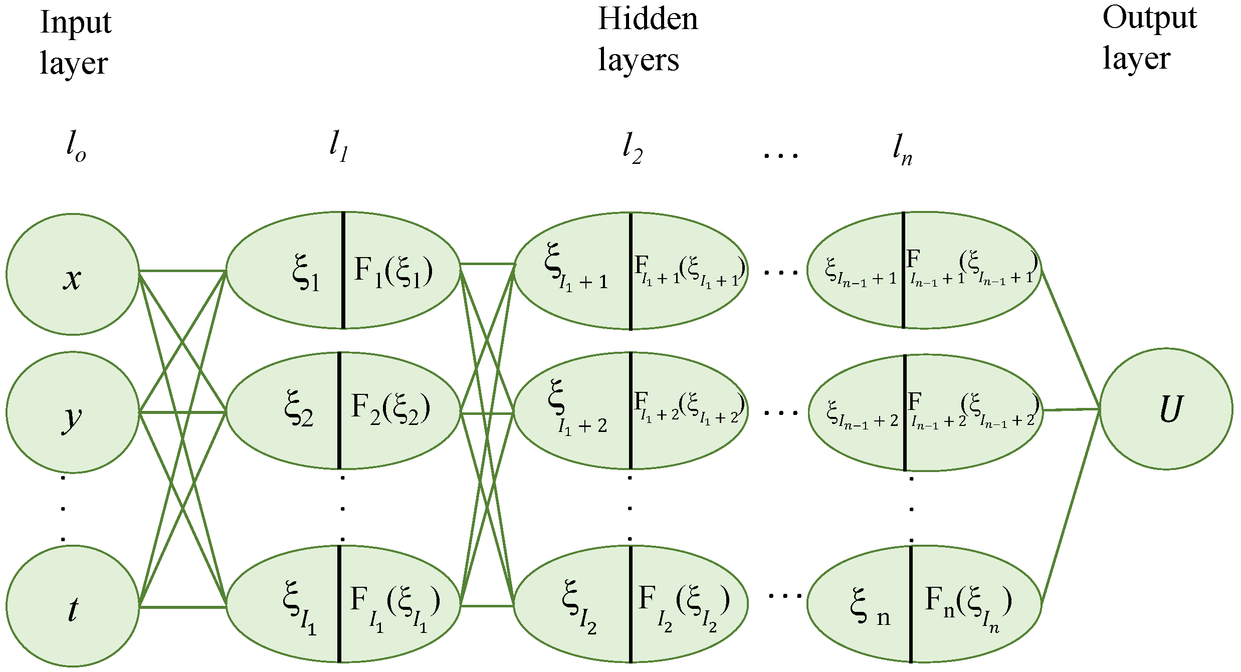
U = ω l n U p F l p ( ξ l p ) ,
where ω l n U is the weight connecting the last hidden layer l n to the output, and F is an activation function. The network incorporates adjustable weights ( ω i p ) and biases ( b m ) from preceding layers. The internal variable ξ l p at the l p t h evolves as:
ξ l p = b m p + ω l p 1 , l p F l p 1 ξ l p 1 , p = 1 , 2 , , n .
with
l k = { x , y , , t } ( k = 2 , 3 , , n 1 ) .
In this framework, forward propagation governs the flow of information from the input layers through the hidden layers to the output layer. At the final stage, the network produces the ultimate result by applying the activation function to the weighted sum of neuronal inputs.
The proposed neural network model is successfully shown in Figure 2.

MGREMM Neural Network

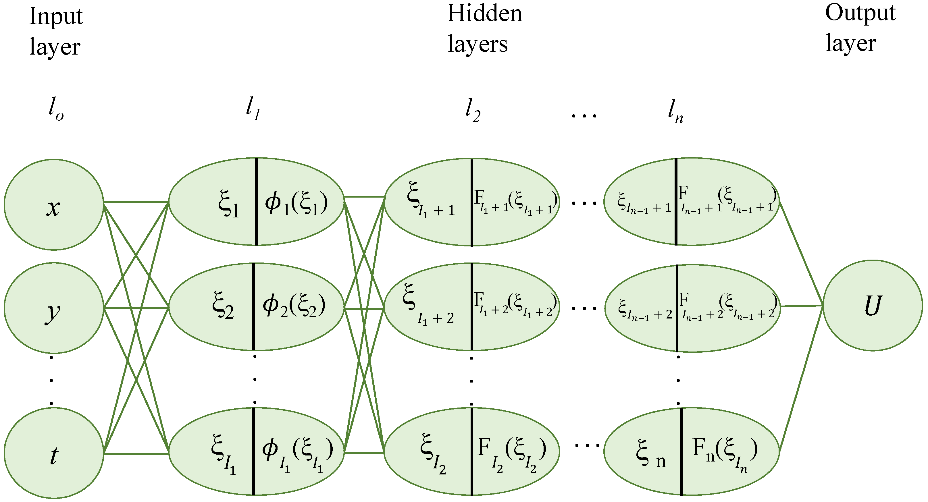
A distinctive hybrid approach, termed the MGREMNN method, integrates the MGREM technique with a neural network model. The core principle of MGREMNN approach lies in utilizing the activation functions of the first hidden layer to realize the analytical MGREM technique. Following the previously outlined steps, a trial function is constructed to transform the partial PDE into an equivalent system of algebraic equations. The solutions obtained via the MGREM method are then employed to design the neural network, specifically defining the activation functions of the first hidden layer. This synergy enables the method to yield exact solutions to PDEs. The fundamental steps constituting the proposed technique are as follows:
Step-1: 
First, we must ensure that the Riccati equation needs modification. We can do this by combining the above-mentioned analytical method with the hidden activation functions of the neural network model.
Step-2: 
To create a model of the proposed neural network, we need the activation function for the hidden layer, as stated previously. The method allows simplifying the selection criterion for the next hidden layer, with the input variables x , t , respectively. The feed-forward method can be then used for the output. This is clearly demonstrated in Figure 3 (the neural network model).
Step-3: 
Likewise, forward-propagation of the proposed neural network architecture may also be used to approximate the trial functions of the PDE.
Step-4: 
Adding the neural network method’s trial functions to the partial differential equations formulates the system of algebraic equations.
Step-5: 
We use algebraic equations with variables x, y, t in conjunction with the function F ( x , t ) , to explore diverse alternative solutions. One way to obtain a set of algebraic equations is to take the coefficients of each term in the equations from Step 4 to zero. This results in the system of equations.
Step-6: 
These algebraic equations must be analyzed in order to determine if evaluating coefficients is justified and meets the requirements. To obtain the first explicit solutions of the function U, these parameters must be substituted into the trial function.
This method finds more exact solutions by training the initial hidden layer of neural networks with an appropriate number of neurons (MGREMM solutions).

3. Studied Equation and Application of the Neural Networking Method

3.1. Governing Equation

The mathematical modeling of wave propagation in microstructured materials (e.g., alloys and ceramics) has emerged as a compelling area of study encompassing multiple microstructural scales [45]. In particular, nonlinear equations are used to develop multi-scale wave propagation models for these materials. Micro strain waves in micro structured materials as described by the NLPDE [46,47,48] read as
U t t U x x α h 1 U 2 x x η h 2 U x x t + δ h 3 U x x x + η 2 h 7 δ h 4 U x x t t + η δ h 5 U x x x x t + h 6 U x x x t t = 0 ,
where U = U ( x , t ) represents the micro strain function and the symbols h k , k = 1 , 2 , 3 , 4 , 5 , 6 , 7 are arbitrary constants with η , δ , represent the dissipative effects, the ratio between micro structure size and wave length and the elastic strain, respectively. Where the subscripts x and t are the partial derivatives. Moreover, the α is a dimensionless perturbation parameter that characterizes the strength of nonlinearity relative to linear wave propagation. It scales the nonlinear and dispersive terms arising from microstructural effects. Specifically, when α is small, the system is weakly nonlinear; when α is of order unity, fully nonlinear behavior emerges. The modeling of traveling waves in these materials illustrates a variety of micro structural characteristics and scales. Furthermore, the dispersive and nonlinear effects may be balanced when the material has nonlinear characteristics. Consequently, these effects may be equilibrated by setting δ = O ( α ) , whereas η = 0 represents the non-dissipative situation, and the double dispersive equation is expressed as
U t t U x x α h 1 ( U 2 ) x x h 3 U x x x x + h 4 U x x t t = 0 .
Additionally, the model under consideration has been examined from a variety of approaches in the literature. The generalized exponential rational function approach was used in [46] to obtain soliton solutions, while the G G 2 -expansion method was used in [47] for finding a variety of soliton solutions. Additionally, the F-expansion approach was used in [48] to examine the suggested model. Moreover, the investigated model represents a strain wave equation for wave propagation in micro structured solids. Due to their internal architecture such as periodic lattices, granular assemblies, or composite micro structures these materials exhibit unusual and often counter intuitive wave behavior beyond the scope of classical continuum theories. Our neural network-based analytical framework yields soliton solutions corresponding to localized, shape-conserving strain waves that propagate without dispersion or dissipation. These nonlinear coherent structures have far-reaching consequences across numerous engineering and physical fields. In mechanical metamaterials, these solitons are the localized deformation pulse propagation with controlled propagation, which can be used to create innovations in impact mitigation, vibration isolation, and mechanical logic devices where information is carried by solitary waves instead of electronic signals. In non-destructive assessment and structural health surveillance, the presence and stability of soliton solutions offers a theoretical foundation to the interpretation of nonlinear wave signatures which arise due to micro structural damage or degradation and enables an inspector to predict the presence of an imminent failure well before macroscopic cracks are formed. The model, in geophysics and seismology, provides information on the mechanics of strain waves traveling through heterogeneous crustal materials, with micro structural effects, including, but not limited to, grain boundaries, fractures, and inclusions, changing the insights into wave dynamics which in turn improve our perceptions of earthquake rupture propagation and ground motion prediction. Moreover, in additive manufacturing and in high fidelity composites, where now routinely precisely engineered micro structures are being fabricated, our analysis platform now offers designers predictive power to design wave propagation behaviour by tactically controlling micro structural architecture. Outside of these direct applications, the soliton solutions themselves possess profound physical implications: they describe the formation of coherent energy transport in otherwise disordered and chaotic systems, and they indicate how small scale heterogeneities can create large scale structure and predictability. The fact that such systems are soliton-soluble requires no more than a mathematical challenge but opens the door to the next generation of wave-controllable hardware, including acoustic diodes and topological insulators as well as programmable mechanical computers. Moreover, bright, dark, and kink solitons are governed by nonlinearity h 1 and dispersion h 3 , h 4 in micro structured solids. Increasing h 1 sharpens and amplifies bright solitons (strain localization in granular chains), while larger h 3 or h 4 broadens them (ultrasonic testing of ceramics). Dark solitons emerge when h 1 becomes defocusing, with larger | h 1 | deepening the dip; kink solitons steepen with higher h 1 and smooth with higher h 3 , h 4 (phase boundaries in polycrystals). These insights enable tailoring grain size and porosity for vibration damping, energy harvesting, and non-destructive evaluation. In this research, we use a powerful and newly developed neural network technique to analyze the soliton solutions of Equation (4).

3.2. Extraction of the Solutions with Neural Network Method

Wave propagation in micro structured materials described by an NLPDE is assessed here using the 2-2-2-1 MGREMNN model, which employs U as the trial function for finding solutions for the proposed model. The model’s output equation U represents the trial function for PDE solutions, and two neurons represent the input and hidden layers of the model, such as
U = ω 3 U F 3 ( ξ 3 ) + ω 4 U F 4 ( ξ 4 ) 2 + b 5 ,
where
ξ 1 = t ω t 1 + x ω x 1 + b 1 , ξ 2 = t ω t 2 + x ω x 2 + b 2 , ξ 3 = ω 13 F 1 ξ 1 + ω 23 F 2 ξ 2 + b 3 , ξ 4 = ω 14 F 1 ξ 1 + ω 24 F 2 ξ 2 + b 4 .
The activation functions are F p ( p = 1 , 2 , 3 , 4 ), the bias terms are b m ( m = 1 , 2 , 3 , 4 , 5 ), and the network weights are ω κ β with κ { t , x , 1 , 2 , 3 , 4 } and β { 1 , 2 , 3 , 4 , U } .
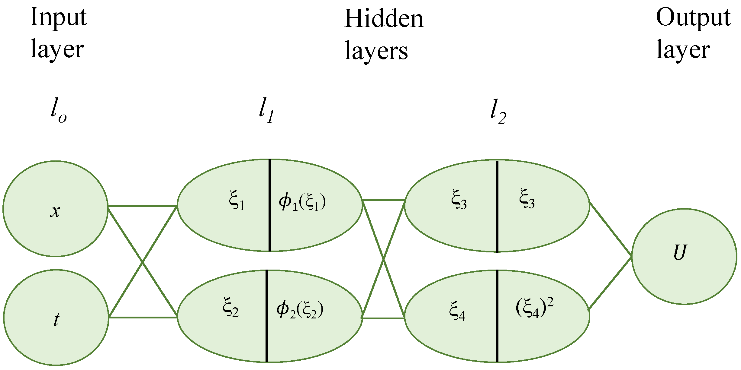
We use the 2-2-2-1 MGREMNN methodology for simplifying the process of computation. The activation functions for the first hidden layer are ϕ ( · ) , which represent the solutions to the Riccati equation. The relevant inputs are x and t. Two functions, ( · ) and ( · ) 2 , serve as activation functions for the second layer. The trial function of the PDE is the output of this neural network, and the results indicate:
U = ω 3 U ( ξ 3 ) + ω 4 U ( ξ 4 ) 2 + b 5 ,
where
ξ 1 = x ω x 1 + t ω t 1 + b 1 , ξ 2 = x ω x 2 + t ω t 2 + b 2 , ξ 3 = ω 13 ϕ ξ 1 + ω 23 ϕ ξ 2 + b 3 , ξ 4 = ω 14 ϕ ξ 1 + ω 24 ϕ ξ 2 + b 4 .
A brief description of the 2-2-2-1 MGREMNN model is given in Figure 4. For simplification of the calculation, in the actual computation, assign b 1 = b 2 = b 3 = b 4 = 0 and b 5 = b . The 2-2-2-1 MGREMNN model’s formula is:
U = ω 3 U ω 13 ϕ x ω x 1 + t ω t 1 + ω 23 ϕ x ω x 2 + t ω t 2 + ω 4 U ω 14 ϕ x ω x 1 + t ω t 1 + ω 24 ϕ x ω x 2 + t ω t 2 2 + b .

3.3. Extraction of Solutions

In this section the proposed method is applied to derive the solution in the form of soliton for the micro strain wave in microstructured solids. The solution to the above system of algebraic equations and using Equation (9) in Equation (4) is as follows:
  • (I) When = 1 2 4 0 2 > 0 , 1 2 0 , 0 2 0 , and ω 14 = 0 , ω 13 = 0 , h 3 = h 1 ω 24 2 ω 4 U 6 2 2 ω x 2 2 + h 4 ,   b = ω 24 2 1 2 + 8 0 2 ω 4 U 12 2 2 , ω 3 U = ω 24 2 1 ω 4 U ω 23 2 , ω t 2 = ω x 2 , then the following solutions are extracted:
  • The dark soliton solution
    U 1 ( x , t ) = ω 24 2 1 2 + 8 0 2 ω 4 U 12 2 2 ω 24 2 1 ω 4 U tanh 1 2 x ω x 2 t ω x 2 + 1 2 2 2 + ω 24 2 ω 4 U tanh 1 2 x ω x 2 t ω x 2 + 1 2 4 2 2 .
  • The explicit solitary wave solutions
    U 2 ( x , t ) = ω 24 2 ω 4 U 3 coth 2 1 2 ( t x ) ω x 2 2 1 2 + 8 0 2 12 2 2 ,
    U 3 ( x , t ) = ω 24 2 ω 4 U sinh ( x t ) ω x 2 + 5 i 12 2 2 sinh ( t x ) ω x 2 + i ,
    U 4 ( x , t ) = ω 24 2 ω 4 U cosh ( x t ) ω x 2 + 5 csc h 2 1 2 ( x t ) ω x 2 24 2 2 .
  • When ω 14 = 0 , ω 13 = 0 , h 3 = 6 h 4 ω t 2 2 + h 1 ω 24 2 ω 4 U 2 2 6 ω x 2 2 , ω x 1 = 0 , b = 1 12 6 ω t 2 2 ω x 2 2 α h 1 ω x 2 2 + ω 24 2 1 2 + 8 0 2 ω 4 U 2 2 ,   ω 3 U = ω 24 2 1 ω 4 U ω 23 2 , we get the different type of soliton solutions as follows:
    U 5 ( x , t ) = ω 24 2 ω 4 U cosh ( x t ) ω x 2 + 5 csc h 2 1 2 ( x t ) ω x 2 24 2 2 ,
    U 6 ( x , t ) = ( ω 24 2 ω 4 U ( c 2 cosh 2 ( x t ) ω x 2 + 11 c 2 8 c d sinh ( x t ) ω x 2 + 2 d 2 12 c c 2 + d 2 cosh ( x t ) ω x 2 ) ) 24 2 2 c sinh ( x t ) ω x 2 + d 2 ,
    U 7 ( x , t ) = ω t 2 2 ω x 2 2 2 α h 1 ω x 2 2 + ( ( 12 c c 2 + d 2 cosh t ω t 2 + x ω x 2 + 2 d 2 + c 2 cosh 2 t ω t 2 + x ω x 2 + 11 8 c d sinh t ω t 2 + x ω x 2 ) ω 24 2 ω 4 U ) 24 2 2 c sinh t ω t 2 + x ω x 2 + d 2 ,
    U 8 ( x , t ) = 1 12 6 ω t 2 2 ω x 2 2 α h 1 ω x 2 2 + ω 24 2 ω 4 U 1 sinh t ω t 2 + x ω x 2 + cosh t ω t 2 + x ω x 2 10 0 2 2 2 1 cosh 1 2 t ω t 2 + x ω x 2 sinh 1 2 t ω t 2 + x ω x 2 2 .
  • When ω 14 = 0 , ω 13 = 0 , h 3 = h 1 ω 24 2 ω 4 U 6 2 2 ω x 2 2 + h 4 , b = ω 24 2 1 2 + 8 0 2 ω 4 U 12 2 2 , ω 3 U = ω 24 2 1 ω 4 U ω 23 2 , ω t 2 = ω x 2 , then we get
    U 9 ( x , t ) = ω 24 2 ω 4 U 1 sinh ( x t ) ω x 2 + cosh ( x t ) ω x 2 + 10 0 2 12 2 2 1 sinh 1 2 ( t x ) ω x 2 + cosh 1 2 ( t x ) ω x 2 2 ,
    U 10 ( x , t ) = 1 12 ω 24 2 ω 4 U 1 2 2 2 + 24 0 1 cosh ( x t ) ω x 2 2 1 cosh ( x t ) ω x 2 + sinh ( x t ) ω x 2 + i + 8 0 1 2 + 6 0 cosh 2 ( x t ) ω x 2 1 cosh ( x t ) ω x 2 sinh ( x t ) ω x 2 + i 2 ,
    U 11 ( x , t ) = ω 24 2 ω 4 u 1 sinh ( x t ) ω x 2 + 1 2 cosh ( x t ) ω x 2 2 0 2 cosh ( x t ) ω x 2 5 12 2 2 1 sinh 1 2 ( t x ) ω x 2 + cosh 1 2 ( t x ) ω x 2 2 .
  • Graphical representation of the solutions with applications
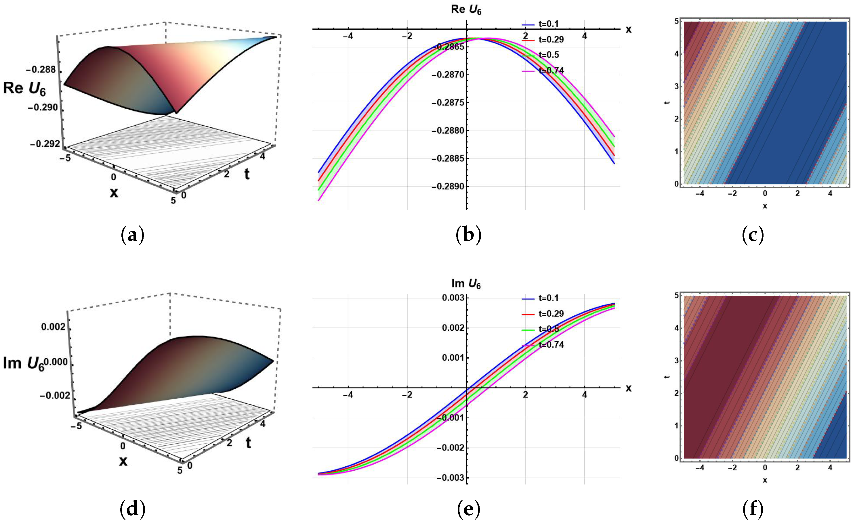
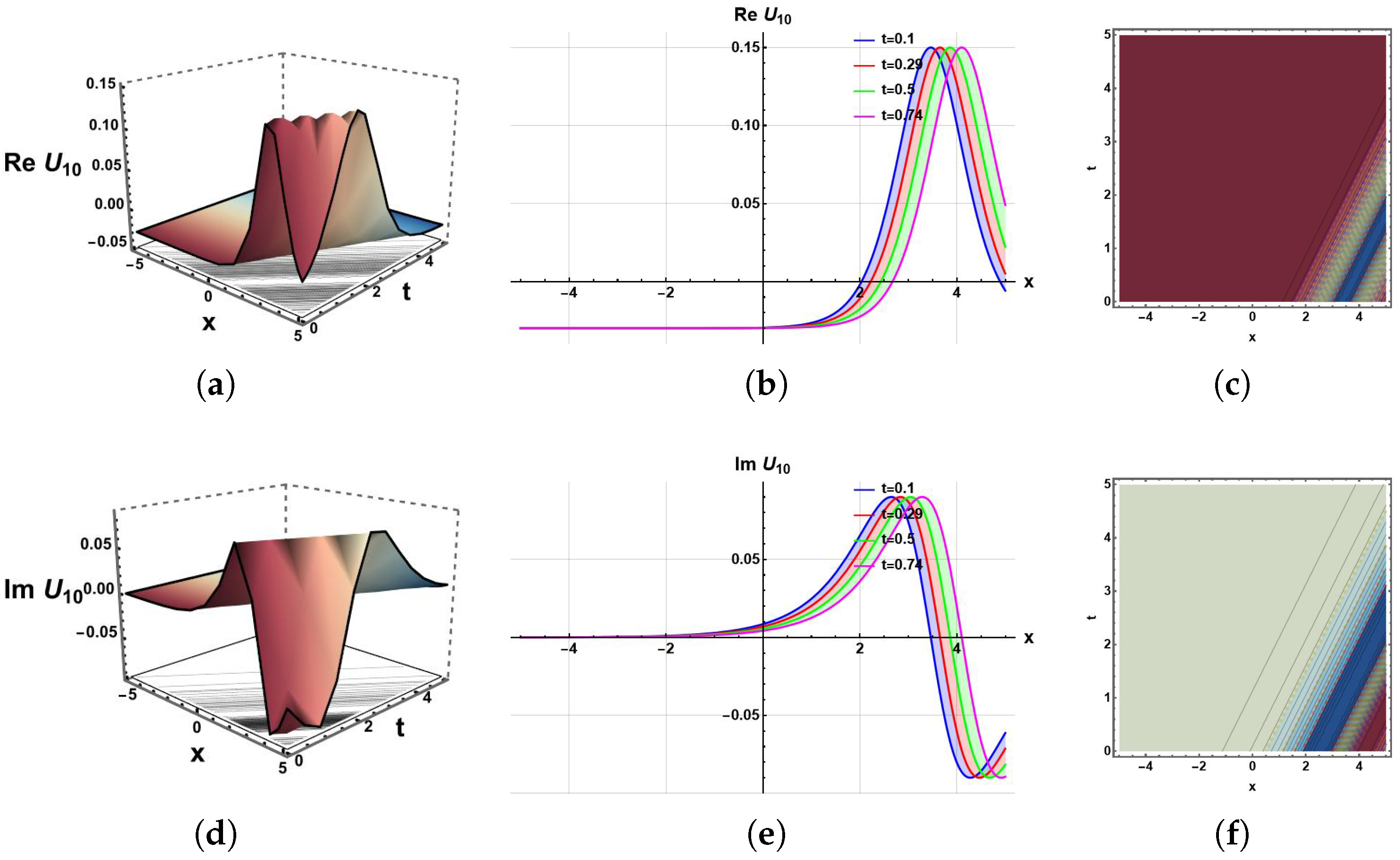
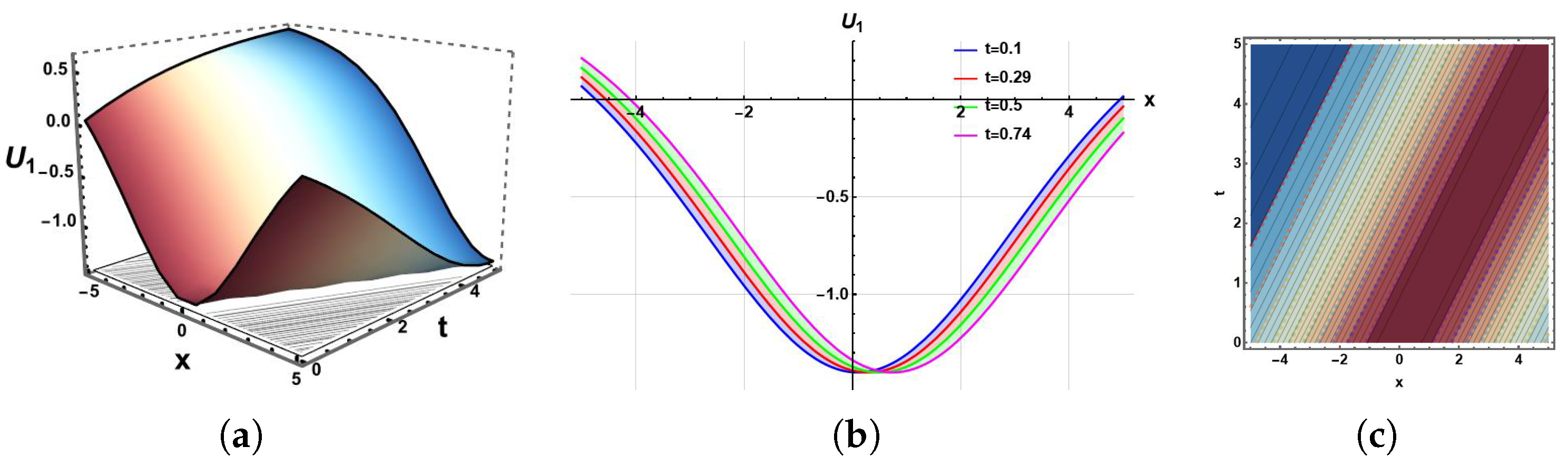
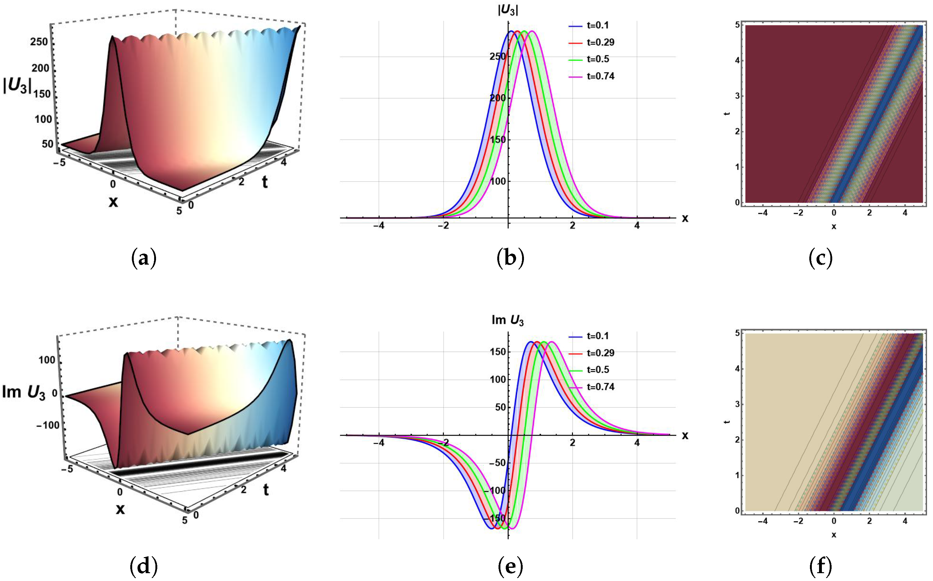
  • In the following, several soliton structures are illustrated in Figure 5, Figure 6, Figure 7 and Figure 8 and their dynamical properties are investigated. These illustrations offer fresh viewpoints on the higher-order influence effects in nonlinear dispersive wave behaviors. Results are presented as a range of different visual representations such as 3D, 2D and contour plots. Here, we explain and explore some of the solutions obtained. The Figure 5 is plotted for the parametric values ω 24 = 0.23 , 1 = 0.991 , 0 = 0.1 , 2 = 0.12 , ω 4 U = 2.45 , ω x 2 = 0.49 to the solution (10) and it show the dynamics of the dark soliton. Dark solitons enable robust energy transport and defect tolerance in microstructured solids. Dark localized wave packet of low intensity on a continuous-wave family occurs in defocusing media. They underpin advanced photonic and phononic functionalities essential for next-generation devices. The Figure 6 represent the bright and combined bright-dark type soliton behaviour to the solution (12) for the values ω 24 = 2.3 , 1 = 1.56 , 0 = 0.01 , 2 = 0.2 , ω 4 U = 2.1 , ω x 2 = 0.93 . Bright solitons enable intense, self-guided energy packets for precise control of light and sound in microstructures. The combined soliton signifies compound interactions between dark and bright modes, elucidating linked wave phenomena and multi-component systems. Moreover, the kink and bright soliton solutions are plotted in the Figure 7 for the solution (15) with the values c = 0.002 , d = 1.2 , ω 24 = 0.3 i , 1 = 0.76 , 0 = 0.1 , 2 = 0.2 , ω 4 U = 3.1 , ω x 2 = 0.39 i . Kink solitons mediate topological phase transitions and stable domain walls in microstructured solids. They are crucial for robust information storage and switching in metamaterials and electronic systems. The values ω 24 = 0.3 i , 1 = 0.6 , 0 = 0.1 , 2 = 0.09 , ω 4 U = 0.1 , ω x 2 = 1.9 are for the Figure 8 to the solution (19).
Figure 5. Plots to the solution (10).
Mathematics 14 02238 g005
Figure 6. Plots to the solution (12).
Mathematics 14 02238 g006
Figure 7. Plots to the solution (15).
Mathematics 14 02238 g007
Figure 8. Plots to the solution (19).
Mathematics 14 02238 g008
  • (II) When = 1 2 4 0 2 < 0 , 1 2 0 , 0 2 0 , and ω 14 = 0 , ω 13 = 0 , h 3 = 6 h 4 ω t 2 2 + h 1 ω 24 2 ω 4 U 2 2 6 ω x 2 2 , ω x 1 = 0 , b = 1 12 6 ω t 2 2 ω x 2 2 α h 1 ω x 2 2 + ω 24 2 1 2 + 8 0 2 ω 4 U 2 2 , ω 3 U = ω 24 2 1 ω 4 U ω 23 2 , then
    U 12 ( x , t ) = ω t 2 2 ω x 2 2 2 α h 1 ω x 2 2 + ω 24 2 ω 4 U cos t ω t 2 + x ω x 2 5 sec 2 1 2 t ω t 2 + x ω x 2 24 2 2 ,
    U 13 ( x , t ) = ω t 2 2 ω x 2 2 2 α h 1 ω x 2 2 ω 24 2 ω 4 U cos t ω t 2 + x ω x 2 + 5 csc 2 1 2 t ω t 2 + x ω x 2 24 2 2 ,
    U 14 ( x , t ) = 1 12 6 ω t 2 2 ω x 2 2 α h 1 ω x 2 2 + ω 24 2 ω 4 U sin t ω t 2 + x ω x 2 + 5 2 2 sin t ω t 2 + x ω x 2 1 ,
    U 15 ( x , t ) = ω 24 2 1 ω 4 U cot t ω t 2 + x ω x 2 + csc t ω t 2 + x ω x 2 + 1 2 2 2 + ω 24 2 ω 4 U cot t ω t 2 + x ω x 2 + csc t ω t 2 + x ω x 2 + 1 2 4 2 2 + 1 12 6 ω t 2 2 ω x 2 2 α h 1 ω x 2 2 + ω 24 2 1 2 + 8 0 2 ω 4 U 2 2 .
  • When ω 14 = 0 , ω 13 = 0 , h 3 = h 1 ω 24 2 ω 4 U 6 2 2 ω x 2 2 + h 4 , b = ω 24 2 1 2 + 8 0 2 ω 4 U 12 2 2 , ω 3 U = ω 24 2 1 ω 4 U ω 23 2 , ω t 2 = ω x 2 , the following solutions may be obtained as:
    U 16 ( x , t ) = ω 24 2 1 ω 4 u tan 1 4 x ω x 2 t ω x 2 cot 1 4 x ω x 2 t ω x 2 2 1 4 2 2 + ω 24 2 1 2 + 8 0 2 ω 4 u 12 2 2 ω 24 2 + 1 16 2 2 ω 4 U tan 1 4 x ω x 2 t ω x 2 cot 1 4 x ω x 2 t ω x 2 2 1 2 ,
    U 17 ( x , t ) = ω 24 2 1 ω 4 U c 2 d 2 c cos x ω x 2 t ω x 2 c sin x ω x 2 t ω x 2 + d 1 2 2 2 + ω 24 2 1 2 + 8 0 2 ω 4 U 12 2 2 + ω 24 2 ω 4 U c 2 d 2 c cos x ω x 2 t ω x 2 c sin x ω x 2 t ω x 2 + d 1 2 4 2 2 ,
    U 18 ( x , t ) = ω 24 2 ω 4 U 1 sin ( x t ) ω x 2 + 1 2 cos ( x t ) ω x 2 2 0 2 cos ( x t ) ω x 2 + 5 12 2 2 1 cos 1 2 ( t x ) ω x 2 sin 1 2 ( t x ) ω x 2 2 ,
    U 19 ( x , t ) = ω 24 2 ω 4 U 1 sin ( x t ) ω x 2 + 1 2 cos ( x t ) ω x 2 2 0 2 cos ( x t ) ω x 2 5 12 2 2 1 sin 1 2 ( t x ) ω x 2 + cos 1 2 ( t x ) ω x 2 2 .
  • When ω 14 = 0 , ω 13 = 0 , h 3 = 6 h 4 ω t 2 2 + h 1 ω 24 2 ω 4 U 2 2 6 ω x 2 2 ,   ω x 1 = 0 , b = 1 12 6 ω t 2 2 ω x 2 2 α h 1 ω x 2 2 + ω 24 2 1 2 + 8 0 2 ω 4 U 2 2 ,   ω 3 U = ω 24 2 1 ω 4 U ω 23 2 , then:
    U 20 ( x , t ) = 1 12 ω 24 2 ω 4 U 1 2 2 2 24 0 1 cos t ω t 2 + x ω x 2 2 1 cos t ω t 2 + x ω x 2 + 2 sin t ω t 2 + x ω x 2 + 1 + 6 ω t 2 2 ω x 2 2 α h 1 ω x 2 2 + 8 0 6 0 cos 2 t ω t 2 + x ω x 2 1 cos t ω t 2 + x ω x 2 + sin t ω t 2 + x ω x 2 + 1 2 + 1 2 ,
    U 21 ( x , t ) = ω t 2 2 ω x 2 2 2 α h 1 ω x 2 2 ( ω 24 2 ω 4 U ( 1 2 cos t ω t 2 + x ω x 2 1 sin t ω t 2 + x ω x 2 2 0 2 cos t ω t 2 + x ω x 2 5 ) ) 12 2 2 1 sin 1 2 t ω t 2 + x ω x 2 cos 1 2 t ω t 2 + x ω x 2 2 ,
  • Graphical representation of the obtained solutions with applications
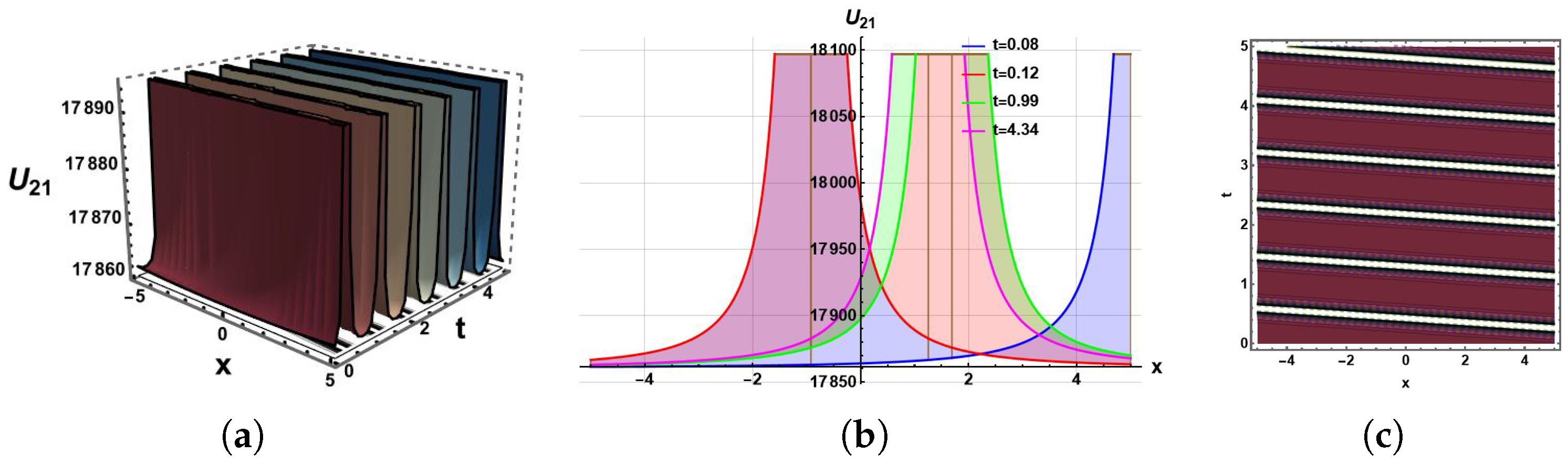
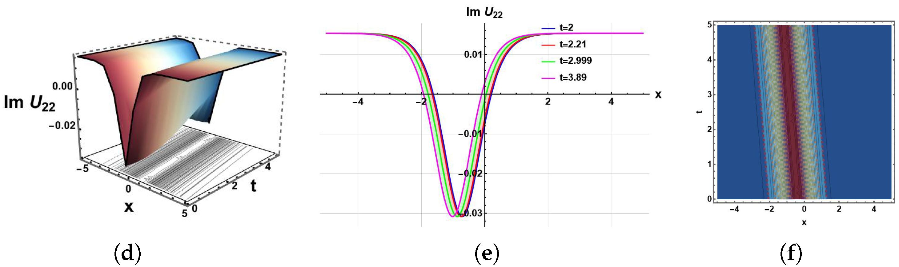
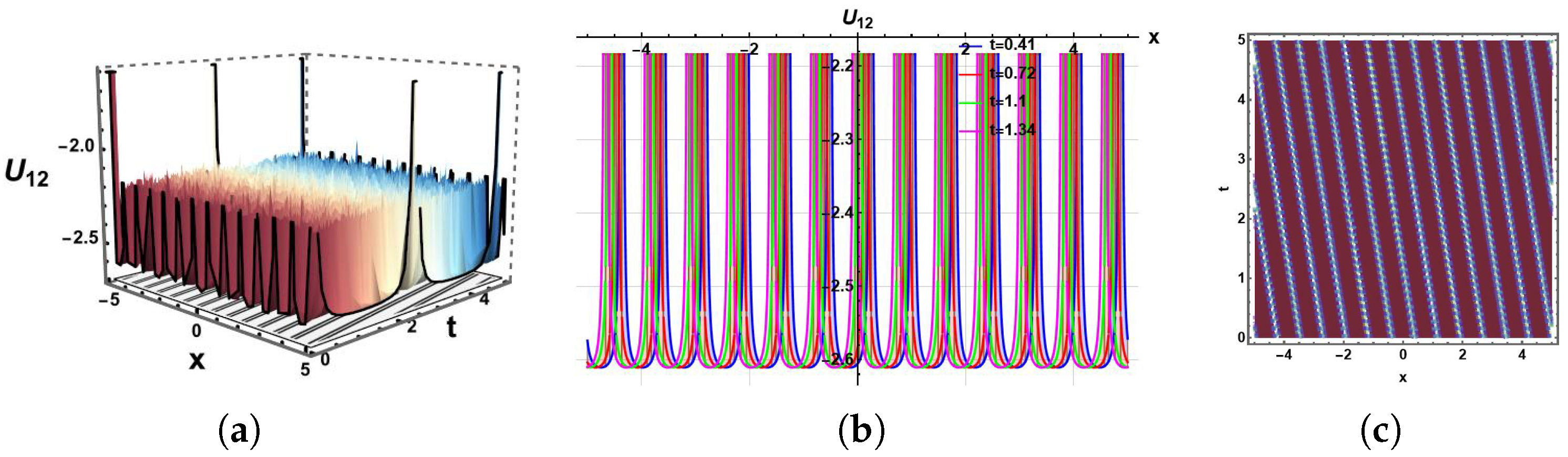
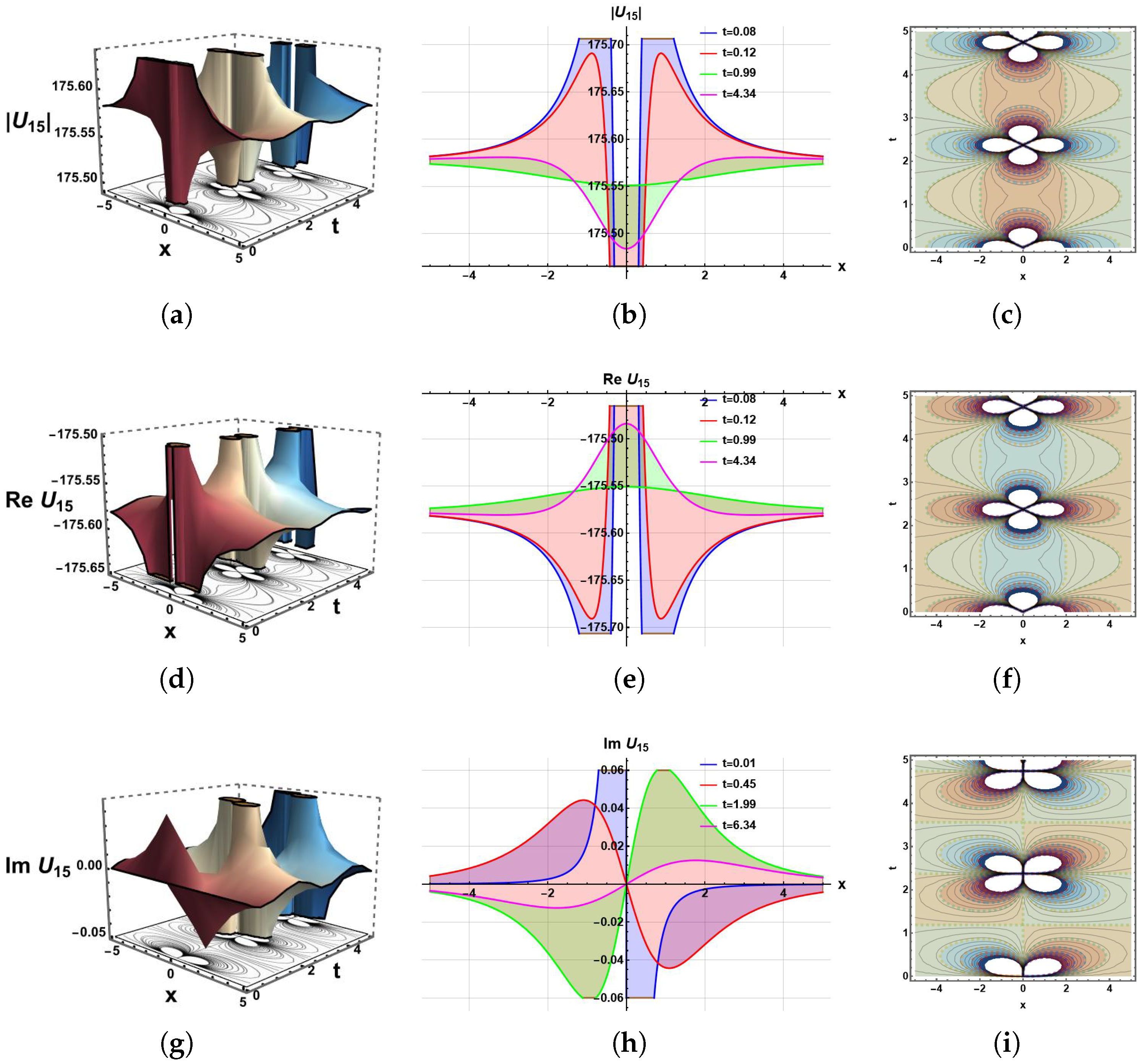
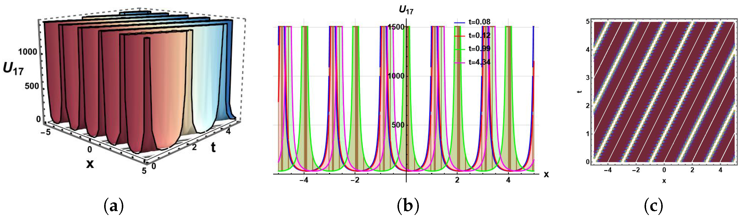
  • The graphical solution of some of the solutions to the equation studied is discussed here. Graphical representation of the solitons is helpful in understanding the dynamic nature, the propagation of the waves and the influence of parametric terms on the solitons. The real, absolute and the imaginary form of the chosen soliton solutions which model the amplitude of the wave is graphically plotted in Figure 9, Figure 10, Figure 11 and Figure 12 over different values of the free parameters in their appropriate ranges. These acquired solutions are presented in 2D, 3D and contour plots, providing a complete picture of the spatial and temporal evolution of the solutions. The periodic behaviour has been observed in the Figure 9 to the solution (21) for the suitable values α = 0.9 , h 1 = 0.19 , ω 24 = 0.1 , 1 = 0.6 , 0 = 1.46 , 2 = 0.9 , ω t 2 = 1.19 ,   ω 4 U = 0.9 , ω x 2 = 3.69 . The dynamics of periodic waves control the propagation of heat, light and sound at the atomic level and determine the core material properties. Their accurate control allows next generation phononic crystals and metamaterials. Moreover, the periodic breather waves that describe energy exchange processes and shows amplitude oscillation are shown in the Figure 10 for the solution (24) with the values α = 0.45 ,   h 1 = 0.12 , ω 24 = 0.1 , 1 = 0.1 , 0 = 2.46 , 2 = 0.9 , ω t 2 = 0.89 , ω 4 U = 0.9 , ω x 2 = 0.21 i . The Figure 11 show the dynamical characteristics of the solution (26) for the values c = 3.35 ,   d = 0.25 , ω 24 = 3.41 , 1 = 0.21 , 0 = 1.06 , 2 = 0.49 , ω t 2 = 0.9 , ω 4 U = 1.9 , ω x 2 = 2.21 . Moreover, the solution (30) is plotted in the Figure 12 with the values α = 0.5 ,   h 1 = 0.05 ,   ω 24 = 3.1 , 1 = 0.1 , 0 = 1.6 , 2 = 0.9 , ω t 2 = 2.99 , ω 4 U = 0.09 , ω x 2 = 0.1 .
Figure 9. Plots to the solution (21).
Mathematics 14 02238 g009
Figure 10. Plots to the solution (24).
Mathematics 14 02238 g010
Figure 11. Plots to the solution (26).
Mathematics 14 02238 g011
Figure 12. Plots to the solution (30).
Mathematics 14 02238 g012
  • (III) When ω 14 = 0 , ω 13 = 0 , h 3 = 6 h 4 ω t 2 2 + h 1 ω 24 2 ω 4 U 2 2 6 ω x 2 2 , ω x 1 = 0 , b = 1 12 6 ω t 2 2 ω x 2 2 α h 1 ω x 2 2 + ω 24 2 1 2 + 8 0 2 ω 4 U 2 2 ,   ω 3 U = ω 24 2 1 ω 4 U ω 23 2 , 0 = 0 , results in the solutions such as:
    U 22 ( x , t ) = 1 12 6 ω t 2 2 ω x 2 2 α h 1 ω x 2 2 + ω 24 2 1 2 ω 4 U 12 Δ 2 Δ sinh 1 t ω t 2 + x ω x 2 + cosh 1 t ω t 2 + x ω x 2 2 12 Δ Δ sinh 1 t ω t 2 + x ω x 2 + cosh 1 t ω t 2 + x ω x 2 + 1 2 2 ,
    U 23 ( x , t ) = 1 12 6 ω t 2 2 ω x 2 2 α h 1 ω x 2 2 + ω 24 2 1 2 ω 4 U 2 2 + ω 24 2 1 2 ω 4 U cosh 1 t ω t 2 + x ω x 2 sinh 1 t ω t 2 + x ω x 2 2 2 2 Δ sinh 1 t ω t 2 + x ω x 2 + cosh 1 t ω t 2 + x ω x 2 2 ω 24 2 1 2 ω 4 U cosh 1 t ω t 2 + x ω x 2 sinh 1 t ω t 2 + x ω x 2 2 2 Δ sinh 1 t ω t 2 + x ω x 2 + cosh 1 t ω t 2 + x ω x 2 ,
    U 24 ( x , t ) = 1 12 6 ω t 2 2 ω x 2 2 α h 1 ω x 2 2 + ω 24 2 1 2 ω 4 U 2 2 + ω 24 2 1 2 ω 4 U sinh 1 t ω t 2 + x ω x 2 + cosh 1 t ω t 2 + x ω x 2 2 2 2 Δ + sinh 1 t ω t 2 + x ω x 2 + cosh 1 t ω t 2 + x ω x 2 2 ω 24 2 1 2 ω 4 U sinh 1 t ω t 2 + x ω x 2 + cosh 1 t ω t 2 + x ω x 2 2 2 Δ + sinh 1 t ω t 2 + x ω x 2 + cosh 1 t ω t 2 + x ω x 2 .
  • Graphical representation of the obtained solutions with applications
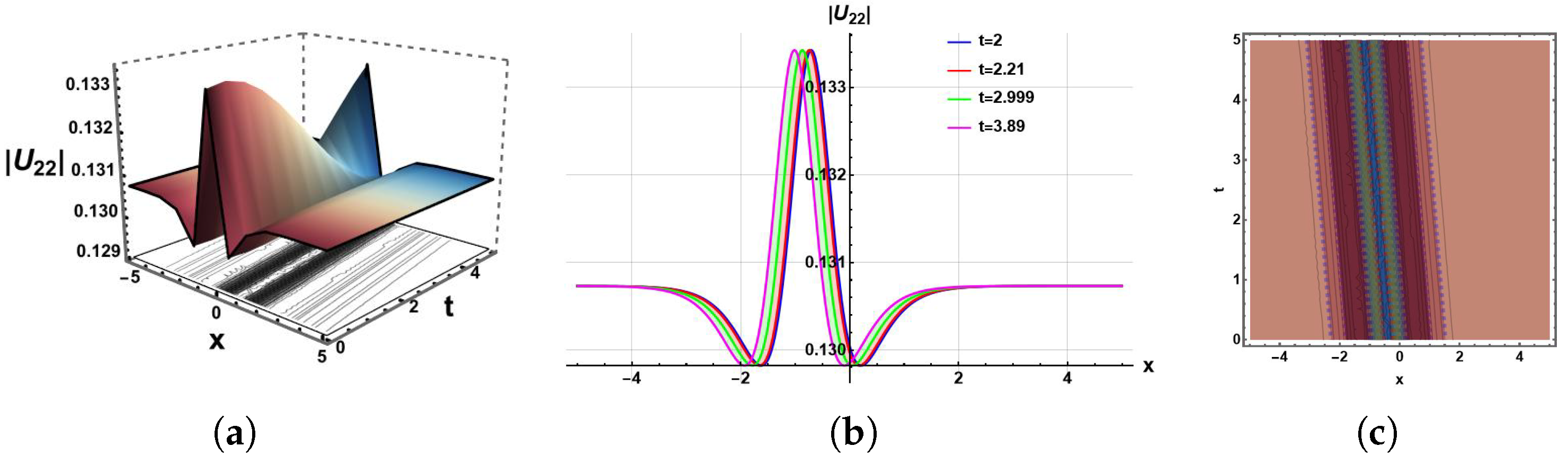
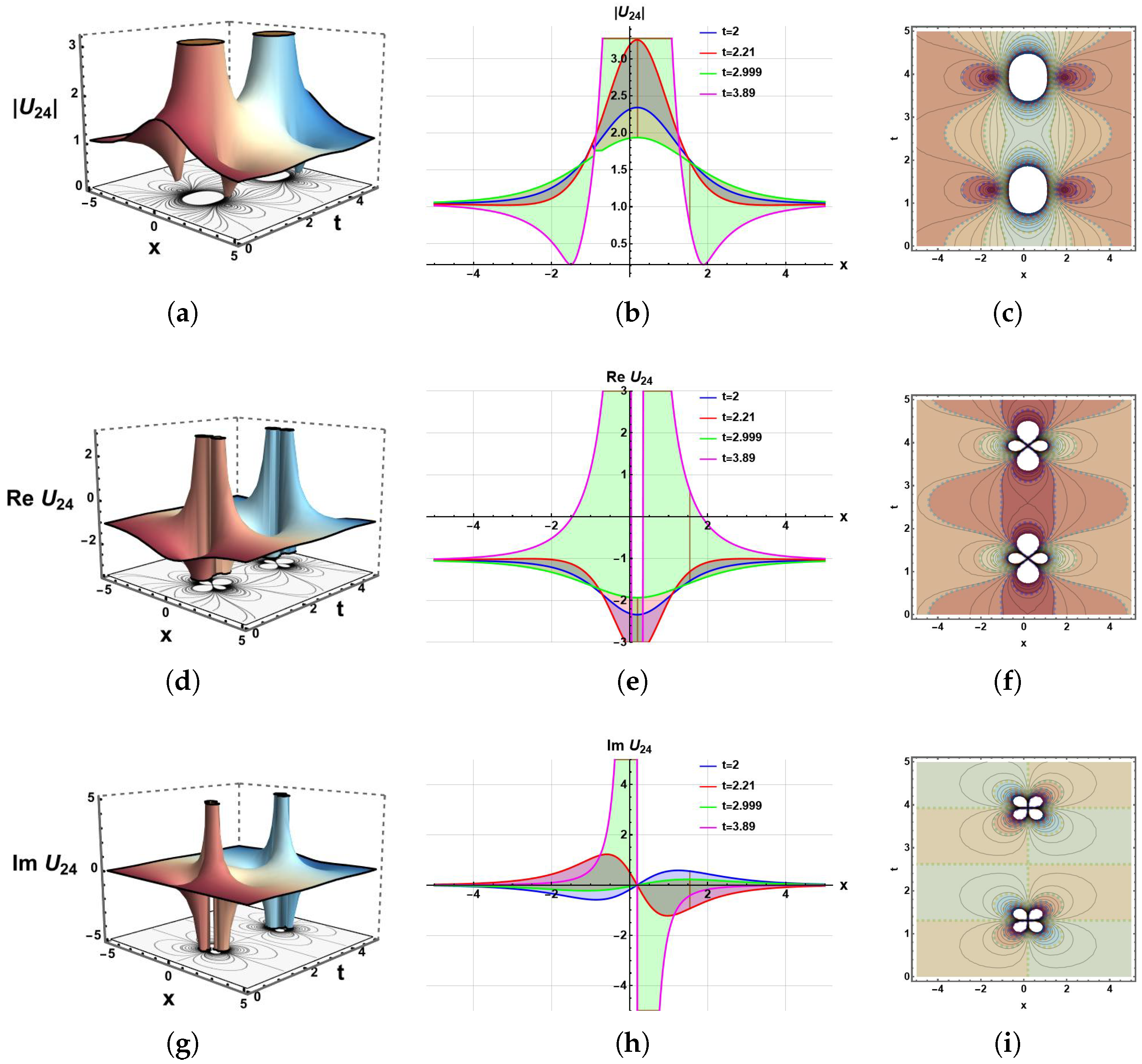
  • Graphical representation compiles complicated data into easy to understand visuals to gain immediate understanding and pattern recognition. It facilitates the exchange of information and human knowledge bringing the ability to communicate well and make a decision quickly. The soliton dynamics is presented in the Figure 13 for the solution (31) with the values α = 1.5 , Δ = 2.6 , h 1 = 2.5 , ω 24 = 2.1 , 1 = 0.41 , 2 = 1.9 , ω t 2 = 0.99 , ω 4 U = 0.9 i , ω x 2 = 6.1 . The lump periodic type dynamics is experienced in the Figure 14 to the solution (33) with the parametric values α = 1.15 , Δ = 1.2 , h 1 = 2.5 , ω 24 = 1.1 , 1 = 0.96 , 2 = 0.561 , ω t 2 = 2.5 i , ω 4 U = 0.9 , ω x 2 = 0.98 . Lump periodic solutions provide a framework for modeling spatially compact, recurring energy packets and localized periodic modes in solid-state systems.
Figure 13. Plots to the solution (31).
Mathematics 14 02238 g013aMathematics 14 02238 g013b
Figure 14. Plots to the solution (33).
Mathematics 14 02238 g014
  • (IV) When ω 14 = 0 , ω 13 = 0 , h 3 = 6 h 4 ω t 2 2 + h 1 ω 24 2 ω 4 U 2 2 6 ω x 2 2 , ω x 1 = 0 , b = 1 12 6 ω t 2 2 ω x 2 2 α h 1 ω x 2 2 + ω 24 2 1 2 + 8 0 2 ω 4 U 2 2 , ω 3 U = ω 24 2 1 ω 4 U ω 23 2 , 0 = 0 , 1 = 0 , we have
    U 25 ( x , t ) = ω t 2 2 ω x 2 2 2 α h 1 ω x 2 2 + ω 24 2 ω 4 U ρ + 2 t ω t 2 + x ω x 2 2 ,
    where Δ , c , d , are real numbers satisfying the condition d 2 c 2 > 0 . The inherent interplay of nonlinearity due to large deformations or material heterogeneity and dispersions due to the characteristic length scale of the micro structure results in a fine balance in micro structured solids which allows solitary waves to be formed. With this balance exactly attained, these isolated waves travel as solitons as localized strain pulses that do not dissipate and do not spread their amplitude, shape or velocity over a long distance. In that matter, the governing strain wave equation has exact soliton solutions, in which the nonlinear term balances the dispersive effects of the micro structure. As a result, every soliton solution is associated with a physically accessible strain wave configuration that is capable of propagation as a stable solution in engineered micro structured materials. This connection is mathematically proven by the fact that the soliton solutions that we derive are the solutions that satisfy the governing partial differential equation with the micro structure parameters coming out clearly in the soliton amplitude, width, and speed. In this way, the solitons that we arrive at are not abstract mathematical objects but that which directly model observable phenomena of strain waves in micro structured mechanical systems of granular chains, lattice metamaterials and composite structures.

4. Conclusions

A new hybrid method called MGREMNN was developed and used to study the dynamics of waves in micro structured solids in this study. The proposed method is a synergy of analytical methods and neural networks which is able to retrieve a variety of analytical solutions, such as solitary wave solutions of the strain wave model describing propagation in microstructured media. Three-dimensional surfaces, contour plots and two-dimensional projections are used to further explain the physical richness of the solutions obtained, and to provide a greater visual understanding into the underlying dynamics of the wave behavior.
One key aspect of MGREMNN differs from traditional analytical processes. A common method is to use a proper transformation to transform the non-linear partial differential equation into an ordinary differential equation and then use a proper analytical method based on a balancing principle. However, the usual approach does not always yield the needed integers to effectively implement the analytical approach. In contrast, MGREMNN overcomes this restriction completely, as it yields solutions directly from the nonlinear equation without having to go through any intermediate transformations or balancing constraints.
The main contribution of this work is to develop soliton theory by using an innovative, intelligent methodology that allows one to create exact solutions with great physical relevance. The obtained solutions have noteworthy stability and long-range persistence features which are very useful for real-world nonlinear wave phenomena modeling. As a result of its efficiency, directness and versatility, the MGREMNN is likely to become a transformative tool in future investigations, providing a powerful and reliable approach to generating soliton solutions to a broad range of the nonlinear evolution equations encountered in mathematical physics and engineering.

Author Contributions

U.Y.: Validation, Investigation, Writing—original draft, Methodology. R.A.A.: Funding acquisition, Software, Formal analysis. F.Y.: Conceptualization, Software, Graphics. J.M.: Resources, Writing—review & editing, Investigation. All authors have read and agreed to the published version of the manuscript.

Funding

This work was supported and funded by the Deanship of Scientific Research at Imam Mohammad Ibn Saud Islamic University (IMSIU) (grant number IMSIU-DDRSP2602).

Data Availability Statement

The article contains all the data that substantiate the results of this research.

Conflicts of Interest

The authors declare no conflicts of interest.

References

  1. Ma, W.X. A matrix integrable enlargement of the DNLS soliton hierarchy incorporating two diagonal matrix blocks. Mathematics 2026, 14, 2081. [Google Scholar] [CrossRef]
  2. Madadi, M.; Inc, M.; Gulsen, S.; Bicer, H.; Akinyemi, L. Determinant solitons and rational lump waves in a (3+1)-dimensional extended Korteweg-de Vries equation. Wave Motion 2026, 147, 103782. [Google Scholar] [CrossRef]
  3. Baloch, S.A.; Mehdi, K.B.; Ali, R.; Siddique, I.; Abduvalieva, D. Exploring solitary wave solutions in the Ivancevic option pricing model using a ϕ6-model fractional derivative technique. J. Nonlinear Complex Data Sci. 2025, 26, 265–287. [Google Scholar]
  4. Sagher, A.A.; Asjad, M.I.; Ullah, N.; Alqarni, M.S. Dynamic solitary waves in the (4+1)-dimensional Davey–Stewartson–Kadomtsev–Petviashvili equation: Exact solutions and sensitivity analysis. Indian J. Phys. 2026, 100, 277–292. [Google Scholar] [CrossRef]
  5. Baloch, A.; Abbas, M.; Abdullah, F.A.; Elamin, M.; Elmahi, M. M-shaped rational, homoclinic breather, kink-cross rational, multi-wave and interactional soliton solutions to the fifth-order Sawada-Kotera equation. Partial Differ. Equ. Appl. Math. 2024, 11, 100919. [Google Scholar]
  6. Chou, D.; Sagher, A.A.; Asjad, M.I.; Hamed, Y.S. Exploring dynamical features like bifurcation assessment, sensitivity visualization, and solitary wave solutions of the integrable Akbota equation. Nonlinear Eng. 2025, 14, 20240040. [Google Scholar] [CrossRef]
  7. Ghergu, M.; Radulescu, V. Nonlinear PDEs: Mathematical Models in Biology, Chemistry and Population Genetics; Springer Science & Business Media: Berlin/Heidelberg, Germany, 2011. [Google Scholar]
  8. Baloch, S.A.; Abbas, M.; Abdullah, F.A.; Rizvi, S.T.R.; Althobaiti, A.; Seadawy, A.R. Multiple soliton solutions of generalized reaction duffing model arising in various mechanical systems. Int. J. Theor. Phys. 2024, 63, 234. [Google Scholar] [CrossRef]
  9. Asjad, M.I.; Sagher, A.A.; Riaz, M.B.; Abdallah, S.A.O. Exploring optical soliton solution for (2+1)-dimensional Kundu–Mukherjee–Naskar equation using two analytical methods with sensitivity analysis. J. Korean Phys. Soc. 2026, 88, 352–369. [Google Scholar] [CrossRef]
  10. Arnous, A.H.; Hosseini, K.; Murad, M.A.S.; Yildirim, Y.; Shah, N.A. Gauge-invariant coherent structures and modulational instability in a stochastic Yajima–Oikawa system. Chaos Solitons Fractals 2026, 210, 118627. [Google Scholar]
  11. Baloch, S.A.; Abbas, M.; Iqbal, M.K.; Birhanu, A.; Alharthi, M.R. Investigation of the new optical soliton solutions to the (2+1)-dimensional calogero-bogoyavlenskii schiff model. Sci. Rep. 2024, 14, 32001. [Google Scholar] [CrossRef] [PubMed]
  12. Sagher, A.A.; Asjad, M.I.; Roshid, M.M.; Abdallah, S.A.O. Exploring soliton and chaotic dynamics in the generalized reaction duffing equation using multiple analytical methods. Model. Earth Syst. Environ. 2025, 11, 232. [Google Scholar] [CrossRef]
  13. Baloch, S.A.; Raza, A.; Moyo, S. Lie symmetry analysis, rogue waves, periodic waves and various analytical solutions of non-linear diffusion equation with applications. Nonlinear Dyn. 2025, 113, 32649–32667. [Google Scholar] [CrossRef]
  14. Barbosa, A.; Sena, J.P.; Kacem, N.; Bouhaddi, N. An artificial intelligence approach to design periodic nonlinear oscillator chains under external excitation with stable damped solitons. Mech. Syst. Signal Process. 2023, 205, 110879. [Google Scholar] [CrossRef]
  15. Onder, I.; Sahiner, A.; Secer, A.; Bayram, M. Soliton solutions of some ocean waves supported by physics informed neural network method. Artif. Intell. Appl. 2024, 2, 280. [Google Scholar] [CrossRef]
  16. Serkin, L.; Belyaeva, T.L. Physics-informed neural networks for higher-rrder nonlinear Schrödinger equations: Soliton dynamics in external potentials. Mathematics 2025, 13, 1882. [Google Scholar]
  17. Amjad, Z.; Farooq, A.; Riaz, H.W.A.; Ma, W.X. Exploring spatiotemporal patterns in the Kuralay–II system using a neural network. Chin. J. Phys. 2026. [Google Scholar] [CrossRef]
  18. Almatrafi, M.; Alharbi, A. New soliton wave solutions to a nonlinear equation arising in plasma physics. Comput. Model. Eng. Sci. 2023, 137, 827. [Google Scholar] [CrossRef]
  19. Soma, M.I.Z.; Islam, T.; Rahman, T.; Ryehan, S. From Hertzian contact to Pochhammer-Chree dynamics: Solitons, chaos, and bifurcation in granular metamaterials. Chaos Solitons Fractals 2026, 208, 118133. [Google Scholar] [CrossRef]
  20. Naschie, M.S.E.; Kapitaniak, T. Soliton chaos models for mechanical and biological elastic chains. Phys. Lett. A 1990, 147, 275–281. [Google Scholar] [CrossRef]
  21. Abdelrahman, M.A.; Refaey, H.A.; Alharthi, M.A. Investigation of new waves in chemical engineering. Phys. Scr. 2021, 96, 075218. [Google Scholar] [CrossRef]
  22. Zabusky, N.J.; Kruskal, M.D. Interaction of “solitons” in a collisionless plasma and the recurrence of initial states. Phys. Rev. Lett. 1965, 15, 240. [Google Scholar] [CrossRef]
  23. Salem, W.K.A.; Fröhlich, J.; Sigal, I.M. Colliding solitons for the nonlinear Schrödinger equation. Commun. Math. Phys. 2009, 291, 151–176. [Google Scholar] [CrossRef][Green Version]
  24. Islam, M.T.; Akter, M.A.; Ryehan, S.; Gómez-Aguilar, J.F.; Akbar, M.A. A variety of solitons on the oceans exposed by the Kadomtsev Petviashvili-modified equal width equation adopting different techniques. J. Ocean Eng. Sci. 2024, 9, 566–577. [Google Scholar]
  25. Liu, H.D.; Tian, B.; Gao, X.T.; Shan, H.W. Integrability and multi-soliton solutions of a variable-coefficient Hirota system and its nonlocal reductions. Eur. Phys. J. Plus 2026, 141, 655. [Google Scholar]
  26. Ye, Y.; Fan, H.; Li, Y.; Liu, X.; Zhang, H. Conformable bilinear neural network method: A novel method for time-fractional nonlinear partial differential equations in the sense of conformable derivative. Nonlinear Dyn. 2025, 113, 7185. [Google Scholar] [CrossRef]
  27. Younas, U.; Muhammad, J.; Ali, Q.; Sediqmal, M.; Kedzia, K.; Jan, A.Z. On the study of solitary wave dynamics and interaction phenomena in the ultrasound imaging modelled by the fractional nonlinear system. Sci. Rep. 2024, 14, 26080. [Google Scholar] [CrossRef] [PubMed]
  28. Islam, M.T.; Alsaud, H.; Rahman, T.; Inc, M. Exclusive soliton solutions arise in mono-mode optical fibre connecting to nonlinear Fokas system. Opt. Quantum Electron. 2024, 56, 753. [Google Scholar] [CrossRef]
  29. Younas, U.; Hussain, E.; Muhammad, J.; Sharaf, M.; Meligy, M.E. Chaotic structure, sensitivity analysis and dynamics of solitons to the nonlinear fractional longitudinal wave equation. Int. J. Theor. Phys. 2025, 64, 42. [Google Scholar] [CrossRef]
  30. Hamad, I.S.; Ali, K.K. Investigation of Brownian motion in stochastic Schrödinger wave equation using the modified generalized Riccati equation mapping method. Opt. Quantum Electron. 2024, 56, 996. [Google Scholar] [CrossRef]
  31. Li, Z. Optical Solutions of the Nonlinear Kodama Equation with the M-Truncated Derivative via the Extended (G′/G)-Expansion Method. Fractal Fract. 2025, 9, 300. [Google Scholar]
  32. Shen, J.; Muhammad, J.; Younas, U. Investigating the wave dynamics and interaction structures: Exploring the Benney-Roskes/Zakharov-Rubenchik model in the oceanic atmosphere. Ocean Eng. 2026, 354, 124969. [Google Scholar]
  33. Muhammad, J.; Younas, U.; Ahmed, K.K. Investigating higher-dimensional nonlinear evolution equation: Dynamics of waves and multistability in fluid mediums. Model. Earth Syst. Environ. 2025, 11, 442. [Google Scholar] [CrossRef]
  34. Islam, M.T.; Rahman, T.; Inc, M.; Akbar, M.A. Comprehensive soliton solutions of fractional stochastic Kraenkel–Manna–Merle equations in ferromagnetic materials. Opt. Quantum Electron. 2024, 56, 927. [Google Scholar]
  35. Li, X.; Shen1, J.; Liang, J.; Gao, Y. Bilinear feature-enhanced symbolic computation neural network method for solving the (1+1)-dimensional Caudrey–Dodd–Gibbon equation. AIMS Math. 2026, 11, 3193–3218. [Google Scholar]
  36. Blechschmidt, J.; Ernst, O.G. Three ways to solve partial differential equations with neural networks—A review. GAMM-Mitteilungen 2021, 44, e202100006. [Google Scholar]
  37. Aarts, L.P.; Veer, P.V.D. Neural network method for solving partial differential equations. Neural Process. Lett. 2001, 14, 261–271. [Google Scholar] [CrossRef]
  38. Chou, D.; Chen, P.Y. A machine learning method to explore the glymphatic system via poroelastodynamics. Chaos Solitons Fractals 2024, 178, 114334. [Google Scholar]
  39. Chou, D.; Chen, P.Y. A perceptron-based learning method for solving the inverse problem of the brain model via poroelastodynamics. Chaos Solitons Fractals 2023, 172, 113611. [Google Scholar] [CrossRef]
  40. Bhattacharya, K.; Hosseini, B.; Kovachki, N.B.; Stuart, A.M. Model reduction and neural networks for parametric PDEs. SMAI J. Comput. Math. 2021, 7, 121–157. [Google Scholar] [CrossRef]
  41. Ruthotto, L.; Haber, E. Deep neural networks motivated by partial differential equations. J. Math. Imaging Vis. 2020, 62, 352–364. [Google Scholar] [CrossRef]
  42. Zhang, R.F.; Bilige, S. Bilinear neural network method to obtain the exact analytical solutions of nonlinear partial differential equations and its application to p-gBKP equation. Nonlinear Dyn. 2019, 95, 3041–3048. [Google Scholar]
  43. Muhammad, J.; Tedjani, A.H.; Hussain, E.; Younas, U. Exploring the exact solutions to the nonlinear systems with neural networks method. Sci. Rep. 2025, 15, 36818. [Google Scholar] [CrossRef] [PubMed]
  44. Kumar, S.; Hamid, I.; Abdou, M.A. Dynamic frameworks of optical soliton solutions and soliton-like formations to Schrödinger–Hirota equation with parabolic law non-linearity using a highly efficient approach. Opt. Quantum Electron. 2023, 55, 1261. [Google Scholar]
  45. Phillips, R. Crystals, Defects and Microstructures: Modeling Across Scales; Cambridge University Press: Cambridge, UK, 2001. [Google Scholar]
  46. Kumar, S.; Kumar, A.; Wazwaz, A.M. New exact solitary wave solutions of the strain wave equation in microstructured solids via the generalized exponential rational function method. Eur. Phys. J. Plus 2020, 135, 870. [Google Scholar] [CrossRef]
  47. Raza, N.; Seadawy, A.R.; Jhangeer, A.; Butt, A.R.; Arshed, S. Dynamical behavior of micro-structured solids with conformable time fractional strain wave equation. Phys. Lett. A 2020, 384, 126683. [Google Scholar] [CrossRef]
  48. Gao, W.; Silambarasan, R.; Baskonus, H.M.; Anand, R.V.; Rezazadeh, H. Periodic waves of the non dissipative double dispersive micro strain wave in the micro structured solids. Phys. A Stat. Mech. Appl. 2020, 545, 123772. [Google Scholar] [CrossRef]
Figure 1. Sequence of the study.
Mathematics 14 02238 g001
Figure 2. Neural network model.
Mathematics 14 02238 g002
Figure 3. MGREMNN model.
Mathematics 14 02238 g003
Figure 4. 2–2–2–1 MGREMNN model of Equation (7).
Mathematics 14 02238 g004
Disclaimer/Publisher’s Note: The statements, opinions and data contained in all publications are solely those of the individual author(s) and contributor(s) and not of MDPI and/or the editor(s). MDPI and/or the editor(s) disclaim responsibility for any injury to people or property resulting from any ideas, methods, instructions or products referred to in the content.