Newton’s Iteration Method for Solving the Nonlinear Matrix Equation $\mathit{X}\mathbf{+}{\mathbf{\sum }}_{\mathit{i}\mathbf{=}\mathbf{1}}^{\mathit{m}}{\mathit{A}}_{\mathit{i}}^{\mathbf{*}}{\mathit{X}}^{\mathbf{-}\mathbf{1}}{\mathit{A}}_{\mathit{i}}\mathbf{=}\mathit{Q}$

Abstract

In this paper, we study the nonlinear matrix equation (NME) $X+{\sum }_{i=1}^m{A}_i^{*}{X}^{-1}{A}_i=Q$. We transform this equation into an equivalent zero-point equation, then we use Newton’s iteration method to solve the equivalent equation. Under some mild conditions, we obtain the domain of approximation solutions and prove that the sequence of approximation solutions generated by Newton’s iteration method converges to the unique solution of this equation. In addition, the error estimation of the approximation solution is given. Finally, the comparison of two well-known approaches with Newton’s iteration method by some numerical examples demonstrates the superiority of Newton’s iteration method in the convergence speed.

1. Introduction

In this paper, we study the properties of solutions and solvability conditions of the nonlinear matrix equation

$$X+\sum _{i=1}^m{A}_i^{*}{X}^{-1}{A}_i=Q,$$

(1)

where $A_i\in {\mathbb{C}}^{n\times n}$ ($i=1,2,\dots ,m$) are given matrices. $A^{*}$ denotes the conjugate transpose of matrix A, Q is a Hermitian positive definite (HPD) matrix, and X is an unknown $n\times n$ matrix to be solved.

In recent years, Equation (1) has attracted extensive attention from researchers. Equation (1) for $m=1$ occurs in control theory, dynamic programming, stochastic filtering, and ladder networks, see more details in [1,2,3,4,5]. Equation (1) for $m=1$ has been well studied in [6,7,8,9]. These results are mainly in the following aspects: sufficient conditions for the existence of HPD solutions, perturbation analysis, condition numbers, and iterative methods for solving the type of equation. Iterative method is a powerful tool for solving various problems, such as matrix equations [10], integral equations [11], variational inequality [12], and image segmentation [13]. In the iterative method, there are mainly fixed-point iteration methods [14] and inversion-free iteration methods [6,15,16,17].

Long et al. gave some sufficient conditions for the existence of an HPD solution of Equation (1) for $m=2$ and proved the convergence of the fixed-point iteration method and inversion-free iteration method used to compute the HPD solution in [18]. Vaezzadeh et al. proposed an iterative method for computing HPD solutions of the matrix equation and gave convergence results for the basic fixed-point iteration for the equations in [19]. Sayevand et al. presented a new inversion-free iteration method to compute a maximal HPD solution for the equation and derived the existence conditions of the nonlinear matrix equation in [20].

Newton’s iteration methods play an important role in computing the nonlinear system and optimization problems. As is known to all, Newton’s iteration method can obtain a quadratic convergence rate under suitable conditions. Hasanov and Hakkaev investigated iterative methods for computing the HPD solution of Equation (1) and provided convergence rates of several fixed-point iterations in [21]. Weng applied Newton’s iteration method to Equation (1) and obtained generalized Stein equations, then he adapt the generalized Smith method to find the HPD solution of Equation (1) in [22]. Huang and Ma proposed some inversion-free iteration methods to compute Equation (1); furthermore, they established Newton’s iteration method to compute the HPD solution and prove its quadratic convergence [23].

Inspired by these works [21,22,23], we further study Equation (1). Although we also use Newton’s iteration method, our method is substantially different from [22,23]. Our method is as follows: when the matrix Q in Equation (1) satisfies some conditions, we can prove that the sequence generated by Newton’s iteration method is contained in an open ball and the sequence converges to the only point in the ball, i.e., the solution of Equation (1).

The remainder of the paper is organized as follows. In Section 2, we illustrate some notations and review some lemmas, which is crucial for achieving our results. In Section 3, we derive the local convergence theorem and prove the sequence generated by Newton’s iteration method converges to an HPD solution of Equation (1). In Section 4, we compare two well-known existing methods: inversion-free iteration and basic fixed-point iteration with Newton’s iteration method by two numerical examples. We conclude in Section 5.

2. Preliminaries

This section includes an explanation of several notations used throughout this paper, a list of some definitions, and lemmas. We use notations ${\mathbb{C}}^{n\times n}$, ${\mathbb{H}}^{n\times n}$ to denote the set of all $n\times n$ complex matrices and all $n\times n$ Hermitian matrices, respectively. For $A\in {\mathbb{C}}^{n\times n}$, we use $\parallel A\parallel$ to denote the spectral norm of A, i.e., $\parallel A\parallel =\sqrt{{\lambda }_{max}\left(A{A}^{*}\right)}$. For $P,Q\in {\mathbb{H}}^{n\times n}$, $P\ge Q$ means $P-Q$ is positive semidefinite. We use notation $A\otimes B$ to denote the Kronecker product of matrices A and B.

The following lemma in [24] is essential for us to establish the convergence theory of Newton’s iteration method for solving Equation (1).

Lemma 1. 

Let $A,B\in {\mathbb{C}}^{n\times n}$ and assume that A is invertible, with $\parallel A^{-1}\parallel \le \alpha$. If $\parallel A-B\parallel \le \beta$ and $\alpha \beta <1$, then B is also invertible, and

$$\parallel B^{-1}\parallel \le \frac{\alpha }{1-\alpha \beta }$$

Proof. 

See [24] (p. 45). □

Lemma 2. 

Let $A\in {\mathbb{C}}^{n\times n}$ and satisfies $\parallel A\parallel <1$, then $I-A$ is nonsingular, then

$${\parallel (I-A)}^{-1}\parallel \le \frac{1}{1-\parallel A\parallel }.$$

Proof. 

See [25] (p. 351). □

3. Newton’s Iteration Method and Its Convergence Analysis for Solving (1)

In this section, we use Newton’s iteration method to solve Equation (1). We prove that the matrix sequence ${\left\{X_k\right\}}_{k⩾0}$ generated by Newton’s iteration method converges to the unique solution of Equation (1) when the initial guess matrix $X_0=Q$ satisfies the following condition

$$\delta \parallel Q^{-1}\parallel <\frac{2}{5},$$

where $\delta :=\frac{2({\sum }_{i=1}^m\parallel A_i{\parallel }^2)\parallel Q^{-1}\parallel }{1-({\sum }_{i=1}^m\parallel A_i{\parallel }^2)\parallel Q^{-1}{\parallel }^2}$. In addition, the error estimation of the approximation solution is given.

3.1. Newton’s Iteration Method

Let

$$F\left(X\right)=X+\sum _{i=1}^m{A}_i^{*}{X}^{-1}{A}_i-Q,$$

(2)

we know $F\left(X\right)$ is Fréchet differentiable at any nonsingular matrix X and we obtain the Fréchet derivative of F at X, denoted by $F_X^{\prime }\left(E\right)$, given as follows

$$F_X^{\prime }\left(E\right)=E-\sum _{i=1}^m{A}_i^{*}{X}^{-1}E{X}^{-1}{A}_i,$$

(3)

Using Newton’s iteration method to solve Equation (1), we obtain

$$X_{k+1}=X_k-{\left(F_{X_k}^{\prime }\right)}^{-1}\left(F\left(X_k\right)\right),k=0,1,2,\dots$$

(4)

where $F_{X_k}^{\prime }$ represents the Fréchet derivative of F at $X_k$. The iteration (4) is equivalent to

$$\begin{array}{cc}\hfill & E_k-\sum _{i=1}^m{A}_i^{*}{X}_k^{-1}{E}_k{X}_k^{-1}{A}_i=-F\left(X_k\right),\hfill \\ \hfill & X_{k+1}=X_k+E_k,k=0,1,2,\dots \hfill \end{array}$$

(5)

or

$$\begin{array}{cc}\hfill X_k-\sum _{i=1}^m{L}_{ik}^{*}{X}_k{L}_{ik}& =Q-2\sum _{i=1}^m{A}_i^{*}{L}_{ik},\hfill \\ \hfill k& =1,2,\dots \hfill \end{array}$$

(6)

where $L_{ik}=X_{k-1}^{-1}{A}_i$, $i=1,2,\dots m$.

Remark 1. 

Iteration (4) is more suitable for convergence analysis in Section 3. However, iteration (6) is more convenient for numerical computation. In order to solve Equation (1), we need to solve the subproblem (6) of Newton’s iteration method; this linear matrix equation could be solved by the iteration method involved in the Stein Equation [21].

Notice that (4) includes inverse operator ${\left(F_X^{\prime }\right)}^{-1}$ at $X_k$, so its properties are crucial for the convergence analysis of iteration (4).

Lemma 3. 

Let $X\in {\mathbb{C}}^{n\times n}$ be nonsingular which satisfies the following inequality

$$(\sum _{i=1}^m\parallel A_i{\parallel }^2)\parallel X^{-1}{\parallel }^2<1,$$

(7)

then the operator $F_X^{\prime }$ is nonsingular, and

$$\parallel {\left(F_X^{\prime }\right)}^{-1}\parallel \le \frac{1}{1-({\sum }_{i=1}^m\parallel A_i{\parallel }^2)\parallel X^{-1}{\parallel }^2}.$$

(8)

Proof. 

$$\begin{array}{cc}\hfill \parallel F_X^{\prime }\left(E\right)\parallel & =\parallel E-\sum _{i=1}^m{A}_i^{*}{X}^{-1}E{X}^{-1}{A}_i\parallel \hfill \\ \hfill & \ge \parallel E\parallel -\parallel \sum _{i=1}^m{A}_i^{*}{X}^{-1}E{X}^{-1}{A}_i\parallel \hfill \\ \hfill & \ge \parallel E\parallel -(\sum _{i=1}^m\parallel A_i{\parallel }^2)\parallel X^{-1}{\parallel }^2\parallel E\parallel \hfill \\ \hfill & =\parallel E\parallel \left[1-(\sum _{i=1}^m\parallel A_i{\parallel }^2)\parallel X^{-1}{\parallel }^2\right].\hfill \end{array}$$

(9)

According to condition (7), $F_X^{\prime }\left(E\right)=0$ if and only if $E=0$. Because $F_X^{\prime }$ is a operator in the finite dimensional vector space ${\mathbb{C}}^{n\times n}$, $F_X^{\prime }$ is an nonsingular operator. Meanwhile

$$\begin{array}{cc}\hfill \parallel {\left(F_X^{\prime }\right)}^{-1}\parallel & =\parallel {\left[I\otimes I-\sum _{i=1}^m{\left(X^{-1}{A}_i\right)}^T\otimes \left(A_i^{*}{X}^{-1}\right)\right]}^{-1}\parallel \hfill \\ \hfill & \le \frac{1}{1-\parallel {\sum }_{i=1}^m{\left(X^{-1}{A}_i\right)}^T\otimes \left(A_i^{*}{X}^{-1}\right)\parallel }\hfill \\ \hfill & \le \frac{1}{1-({\sum }_{i=1}^m\parallel A_i{\parallel }^2)\parallel X^{-1}{\parallel }^2}.\hfill \end{array}$$

(10)

According to Lemma 2, the last inequality holds. □

The next lemma shows that function F satisfies the local Lipschitz conditions.

Lemma 4 

([23]). For any nonsingular matrices $X,Y$ we have

$$\parallel F_X^{\prime }-F_Y^{\prime }\parallel \le (\sum _{i=1}^m\parallel A_i{\parallel }^2\left)\right(\parallel X^{-1}\parallel +\parallel Y^{-1}\parallel )\parallel X^{-1}\parallel \parallel Y^{-1}\parallel \parallel X-Y\parallel .$$

Next, we define a matrix function based on (2) as follows

$$H\left(X\right):={\left(F_Q^{\prime }\right)}^{-1}\left(F\left(X\right)\right).$$

(11)

We notice that Newton’s iteration for $H\left(X\right)$ is consistent with Newton’s iteration for $F\left(X\right)$, i.e.,

$$X_{k+1}-X_k=-{\left(H_{X_k}^{\prime }\right)}^{-1}\left(H\left(X_k\right)\right)=-{\left(F_{X_k}^{\prime }\right)}^{-1}\left(F\left(X_k\right)\right).$$

(12)

Theorem 1. 

Suppose δ and matrix Q satisfy the following inequality

$$\delta \parallel Q^{-1}\parallel <\frac{2}{5},$$

(13)

where $\delta :=\frac{2({\sum }_{i=1}^m\parallel A_i{\parallel }^2)\parallel Q^{-1}\parallel }{1-({\sum }_{i=1}^m\parallel A_i{\parallel }^2)\parallel Q^{-1}{\parallel }^2}$. Furthermore, let $B(Q,\delta )=\{X\mid \parallel X-Q\parallel <\delta \}$. Then, we have the following properties:

(i) $\parallel H\left(Q\right)\parallel \le \frac{\delta }{2}$;

(ii) $\parallel H_X^{\prime }-H_Y^{\prime }\parallel \le \frac{1}{\delta }\parallel X-Y\parallel ,\forall X,Y\in B(Q,\delta )$;

(iii) $\parallel {\left(H_X^{\prime }\right)}^{-1}\parallel \le \frac{1}{1-\parallel X-Q\parallel /\delta },\forall X\in B(Q,\delta )$;

(iv) $\parallel H\left(X\right)-H\left(Y\right)-H_Y^{\prime }(X-Y)\parallel \le \frac{1}{2\delta }{\parallel X-Y\parallel }^2,\forall X,Y\in B(Q,\delta )$;

Proof. 

(i) According to the definition of $\delta$ and (8), we obtain

$$\begin{array}{cc}\hfill \parallel H\left(Q\right)\parallel & =\parallel {(F_Q^{\prime })}^{-1}\left(F\left(Q\right)\right)\parallel \hfill \\ \hfill & \le \parallel {(F_Q^{\prime })}^{-1}\parallel \parallel F\left(Q\right)\parallel \hfill \\ \hfill & \le \frac{({\sum }_{i=1}^m\parallel A_i{\parallel }^2)\parallel Q^{-1}\parallel }{1-({\sum }_{i=1}^m\parallel A_i{\parallel }^2)\parallel Q^{-1}{\parallel }^2}\hfill \\ \hfill & =\frac{\delta }{2}.\hfill \end{array}$$

(14)

□

Proof. 

(ii) Using Lemmas 4 and 1, we have

$$\begin{array}{cc}\hfill \parallel H_X^{\prime }-H_Y^{\prime }\parallel & =\parallel {(F_Q^{\prime })}^{-1}(F_X^{\prime }-F_Y^{\prime })\parallel \hfill \\ \hfill & \le \frac{\parallel F_X^{\prime }-F_Y^{\prime }\parallel }{1-({\sum }_{i=1}^m\parallel A_i{\parallel }^2)\parallel Q^{-1}{\parallel }^2}\hfill \\ \hfill & \le \left[\frac{({\sum }_{i=1}^m\parallel A_i{\parallel }^2\left)\right(\parallel X^{-1}\parallel +\parallel Y^{-1}\parallel )\parallel X^{-1}\parallel \parallel Y^{-1}\parallel }{1-({\sum }_{i=1}^m\parallel A_i{\parallel }^2)\parallel Q^{-1}{\parallel }^2}\right]\parallel X-Y\parallel \hfill \\ \hfill & \le \left[\frac{2({\sum }_{i=1}^m\parallel A_i{\parallel }^2)\parallel Q^{-1}\parallel }{1-({\sum }_{i=1}^m\parallel A_i{\parallel }^2)\parallel Q^{-1}{\parallel }^2}\frac{\parallel Q^{-1}{\parallel }^2}{(1-\delta \parallel Q^{-1}{\parallel )}^3}\right]\parallel X-Y\parallel \hfill \\ & \le \left[\frac{\parallel Q^{-1}{\parallel }^2\delta }{(1-\delta \parallel Q^{-1}{\parallel )}^3}\right]\parallel X-Y\parallel \hfill \\ \hfill & \le \frac{1}{\delta }\left[\frac{\parallel Q^{-1}{\parallel }^2{\delta }^2}{(1-\delta \parallel Q^{-1}{\parallel )}^3}\right]\parallel X-Y\parallel \hfill \\ \hfill & \le \frac{1}{\delta }\parallel X-Y\parallel .\hfill \end{array}$$

(15)

The second and third inequality in (15) are derived from Lemma 4 and Lemma 1, respectively. Due to condition (13), the last inequality in (15) holds. □

Proof. 

(iii) By the definition of $H\left(X\right)$, we have $\parallel {(H_Q^{\prime })}^{-1}\parallel =1$. For all $X\in B(Q,\delta )$, using (ii) we have

$$\parallel H_X^{\prime }-H_Q^{\prime }\parallel \le \frac{1}{\delta }\parallel X-Q\parallel <1,$$

and, according to Lemma 1, we have

$$\parallel {\left(H_X^{\prime }\right)}^{-1}\parallel \le \frac{1}{1-\parallel X-Q\parallel /\delta }.$$

□

Proof. 

(iv) According to the Newton–Leibniz formula and (ii), we obtain

$$\begin{array}{cc}\hfill \parallel H\left(X\right)-H\left(Y\right)-H_Y^{\prime }(X-Y)\parallel & =\parallel {\int }_0^1(H_{(1-t)Y+tX}^{\prime }-H_Y^{\prime })(X-Y)dt\parallel \hfill \\ \hfill & \le \parallel X-Y\parallel {\int }_0^1\parallel (H_{(1-t)Y+tX}^{\prime }-H_Y^{\prime })\parallel dt\hfill \\ \hfill & \le \frac{1}{2\delta }{\parallel X-Y\parallel }^2.\hfill \end{array}$$

□

Theorem 2. 

If the inequality (13) is satisfied, take the initial guess $X_0=Q$, then the sequence ${\left\{X_k\right\}}_{k⩾0}$ generated by Newton’s iteration method for $H\left(X\right)$ belongs to the ball $B(X_0,\delta )$. In addition, we obtain the following inequalities for all $k\ge 1$:

$$\begin{array}{cc}\hfill \parallel X_k-X_{k-1}\parallel \le \frac{\delta }{2^k},& \parallel X_k-X_0\parallel \le \delta (1-\frac{1}{2^k})\hfill \end{array}$$

(16)

$$\begin{array}{cc}\hfill \parallel {(H_{X_k}^{\prime })}^{-1}\parallel \le 2^k,& \parallel \left(H_{X_k}\right)\parallel \le \frac{\delta }{2^{2k+1}}\hfill \end{array}$$

(17)

Proof. 

We first check (16) and (17) when $k=1$. For $X_1=X_0-{(H_{X_0}^{\prime })}^{-1}\left(H\left(X_0\right)\right)=X_0-H\left(X_0\right)$. So we have

$$\parallel X_1-X_0\parallel \le \parallel H\left(X_0\right)\parallel \le \frac{\delta }{2},$$

and

$$\parallel {(H_{X_1}^{\prime })}^{-1}\parallel \le \frac{1}{1-\parallel X_1-X_0\parallel /\delta }\le 2.$$

(18)

According to (iv) in Theorem 1, we obtain

$$\begin{array}{cc}\hfill \parallel (H\left(X_1\right)\parallel & =\parallel (H\left(X_1\right)-H\left(X_0\right)-H_{X_0}^{\prime }(X_1-X_0)\parallel \hfill \\ \hfill & \le \frac{1}{2\delta }{\parallel X_1-X_0\parallel }^2\hfill \\ \hfill & \le \frac{\delta }{2^3}.\hfill \end{array}$$

Suppose inequalities (16) and (17) hold for $k\le s$. We will prove inequalities (16) and (17) hold for $k=s+1$. Because $H_{X_s}^{\prime }$ is nonsingular, then we have $X_{s+1}=X_s-{(H_{X_s}^{\prime })}^{-1}\left(H\left(X_s\right)\right)$. According to mathematical induction and (iii), (iv) in Theorem 1, we have

$$\begin{array}{cc}\hfill \parallel X_{s+1}-X_s\parallel & \le \parallel {(H_{X_s}^{\prime })}^{-1}\parallel \parallel H\left(X_s\right)\parallel \le \frac{\delta }{2^{s+1}},\hfill \\ \hfill \parallel X_{s+1}-X_0\parallel & \le \parallel X_s-X_0\parallel +\parallel X_{s+1}-X_s\parallel \hfill \\ \hfill & =\delta (1-\frac{1}{2^s})+\frac{\delta }{2^{s+1}}\hfill \\ \hfill & =\delta (1-\frac{1}{2^{s+1}}),\hfill \\ \hfill \parallel {(H_{X_{s+1}}^{\prime })}^{-1}\parallel & \le \frac{1}{1-\parallel X_{s+1}-X_0\parallel /\delta }\le 2^{s+1},\hfill \\ \hfill \parallel (H\left(X_{s+1}\right)\parallel & =\parallel H\left(X_{s+1}\right)-H\left(X_s\right)-H_{X_s}^{\prime }(X_{s+1}-X_s)\parallel \hfill \\ \hfill & \le \frac{1}{2\delta }{\parallel X_{s+1}-X_s\parallel }^2\hfill \\ \hfill & \le \frac{\delta }{2^{2s+3}}.\hfill \end{array}$$

Thus, we prove inequalities (16) and (17) hold for $k=s+1$. In addition, according to definition of $B(Q,\delta )$ and inequalities (16), we know the sequence ${\left\{X_k\right\}}_{k⩾0}$ belong to the open ball $B(Q,\delta )$. □

3.2. Convergence Analysis

Theorem 3. 

If inequality (13) is satisfied, take the initial matrix $X_0=Q$, then the sequence ${\left\{X_k\right\}}_{k⩾0}$ generated by Newton’s iteration method for $H\left(X\right)$, which is located in the closed ball $\overline{B(X_0,\delta )}$, converges to a zero $X^{*}$ of $F\left(X\right)$. In addition, the error estimate

$$\parallel X_k-X^{*}\parallel \le \frac{\delta }{2^k},$$

holds for $k\ge 0$.

Proof. 

According to (16) $\parallel X_k-X_{k-1}\parallel \le \frac{\delta }{2^k},k\ge 1$ in Theorem 2, we first prove sequence ${\left\{X_k\right\}}_{k⩾0}$ is a Cauchy sequence.

Given any integer $k\ge 0$, and $l\ge 1$, we have

$$\parallel X_k-X_{k+l}\parallel \le \sum _{i=k}^{k+l-1}\parallel X_{i+1}-X_i\parallel \le \sum _{i=k}^{\infty }\frac{\delta }{2^{i+1}}=\frac{\delta }{2^k}.$$

(19)

thus sequence $\left\{X_k\right\}$ is a Cauchy sequence.

According to Theorem 2, $X_k\in B(X_0,\delta )\subseteq \overline{B(X_0,\delta )}$; obviously $\overline{B(X_0,\delta )}$ is a Banach space, therefore there exists $X^{*}\in \overline{B(X_0,\delta )}$ to satisfy

$$X^{*}=\underset{k\to \infty }{lim}{X}_k.$$

Because function $H\left(X\right)$ is continuous and $\parallel H\left(X_k\right)\parallel \le \frac{\delta }{2^{2k+1}},k\ge 1$, we have

$$H\left(X^{*}\right)=\underset{k\to \infty }{lim}H\left(X_k\right)=0.$$

Thus, by the definition of $H\left(X\right)$, we know $X^{🟉}$ is a zero of $F\left(X\right)$. Taking the limits of l in (19) yields

$$\parallel X_k-X^{🟉}\parallel \le \frac{\delta }{2^k}.$$

□

Theorem 4. 

If the inequality (13) is satisfied, take the initial matrix $X_0=Q$. Then $F\left(X\right)$ has only zero in the closed ball $\overline{B(X_0,\delta )}$.

Proof. 

Suppose there exists $\tilde{Y}\in \overline{B(X_0,\delta )}$ such that $F(\tilde{Y})=0$, we will prove

$$\parallel X_k-\tilde{Y}\parallel \le \frac{\delta }{2^k}$$

(20)

hold for all $k\ge 0$, where $X_k$ are generated by Newton’s iteration for $H\left(X\right)$.

Inequality (20) is true when $k=0$. We assume (20) is true for $k\le s$; next we will prove inequality (20) is true for $k=s+1$. First, we have

$$\begin{array}{cc}\hfill X_{s+1}-\tilde{Y}& =X_s-{(H_{X_s}^{\prime })}^{-1}\left(H\left(X_s\right)\right)-\tilde{Y}\hfill \\ \hfill & =X_s-H(\tilde{Y})-{(H_{X_s}^{\prime })}^{-1}\left(H\left(X_s\right)\right)-\tilde{Y}\hfill \\ \hfill & ={(H_{X_s}^{\prime })}^{-1}[H(\tilde{Y})-H\left(X_s\right)-H_{X_s}^{\prime }(\tilde{Y}-X_s)].\hfill \end{array}$$

Using (iv) in Theorem 1, Theorem 2, and the induction hypothesis, we have

$$\parallel X_{s+1}-\tilde{Y}\parallel \le \parallel {(H_{X_s}^{\prime })}^{-1}\parallel \frac{1}{2\delta }{\parallel \tilde{Y}-X_s\parallel }^2\le \frac{\delta }{2^{s+1}}.$$

Therefore, inequality (20) is true for $k\ge 0$. So

$$\underset{s\to \infty }{lim}\parallel X_s-\tilde{Y}\parallel =\parallel \tilde{X}-\tilde{Y}\parallel =0,$$

(21)

hence, we have $\tilde{Y}=\tilde{X}$. □

4. Numerical Experiments

In this section, in order to illustrate the convergence behaviour of Newton’s iteration method for solving Equation (1), we report some numerical results to solve Equation (1) by Newton’s iteration method (NIM), inversion-free iteration (IFI), and basic fixed-point iteration (BFPI) in [26]. All numerical examples are implemented on a Windows 10 computer with an Intel i5 (1.6 GHz) Processor and 8 GB of RAM; the programming language is MATLAB R2018a. The Frobenius norm of the residual is as follows:

$$Res\left(X_k\right)={\parallel X_k+\sum _{i=1}^m{A}_i^{*}{X}_k^{-1}{A}_i-Q\parallel }_F,$$

where ${\parallel A\parallel }_F=\sqrt{{\sum }_{i,j=1}^m\mid a_{i,j}{\mid }^2}$ for a complex $n\times n$ matrix A. We stop the iterative process if the Frobenius norm of the residual is less than $1\times {10}^{-8}$.

We illustrate some notations used in this section:

• IT is the number of iterations;
• CPU means the iterations’ running times in seconds;
• In [26], the authors solve Equation (1) when $Q=I$ by different methods:
  –IFI—inversion-free iteration;
  –BFPI—basic fixed-point iteration;

In order to use Newton’s iteration method to solve Equation (1), we need to solve subproblem (6) of Newton’s iteration method. The Stein iteration [21] (Algorithm 3.2) is an effective method for solving subproblem (6) of Newton’s iteration method. The Stein iteration is as follows:

Let $X_0=Q$, for $k=1,2,\dots$, take $L_{ik}=X_{k-1}^{-1}{A}_i$, $i=1,2,\dots m$, and solve

$$X_k-L_{jk}^{*}{X}_k{L}_{jk}=Q-\sum _{i=1}^m{A}_i^{*}{L}_{ik}-A_j^{*}{L}_{jk},$$

where j is a fixed index in $\{1,2,\cdots ,m\}$, until $\parallel X_k-X_{k-1}{\parallel }_{\infty }\le tol$. Then $X^{*}\approx X_k$, $X^{*}$ is an HPD solution of Equation (1).

Example 1. 

Consider Equation (1) with

$$A_1=\frac{1}{1200}\left(\begin{array}{ccc}100& -150& -259\\ 15& 212& -64\\ 25& -69& 138\end{array}\right),$$

$$A_2=\frac{1}{1200}\left(\begin{array}{ccc}160& -25& 20\\ -25& -288& -60\\ 4& -16& -120\end{array}\right).$$

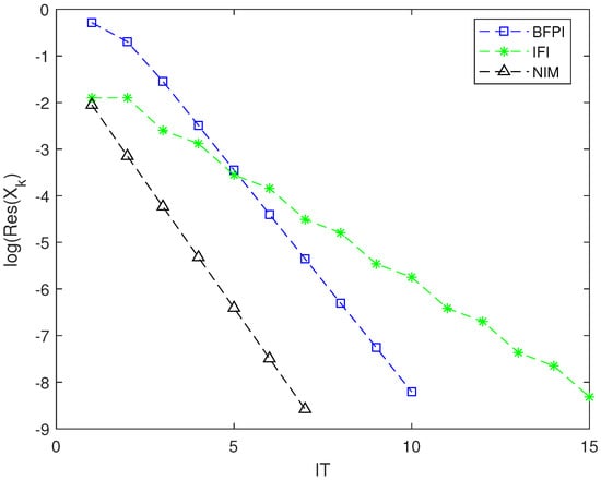
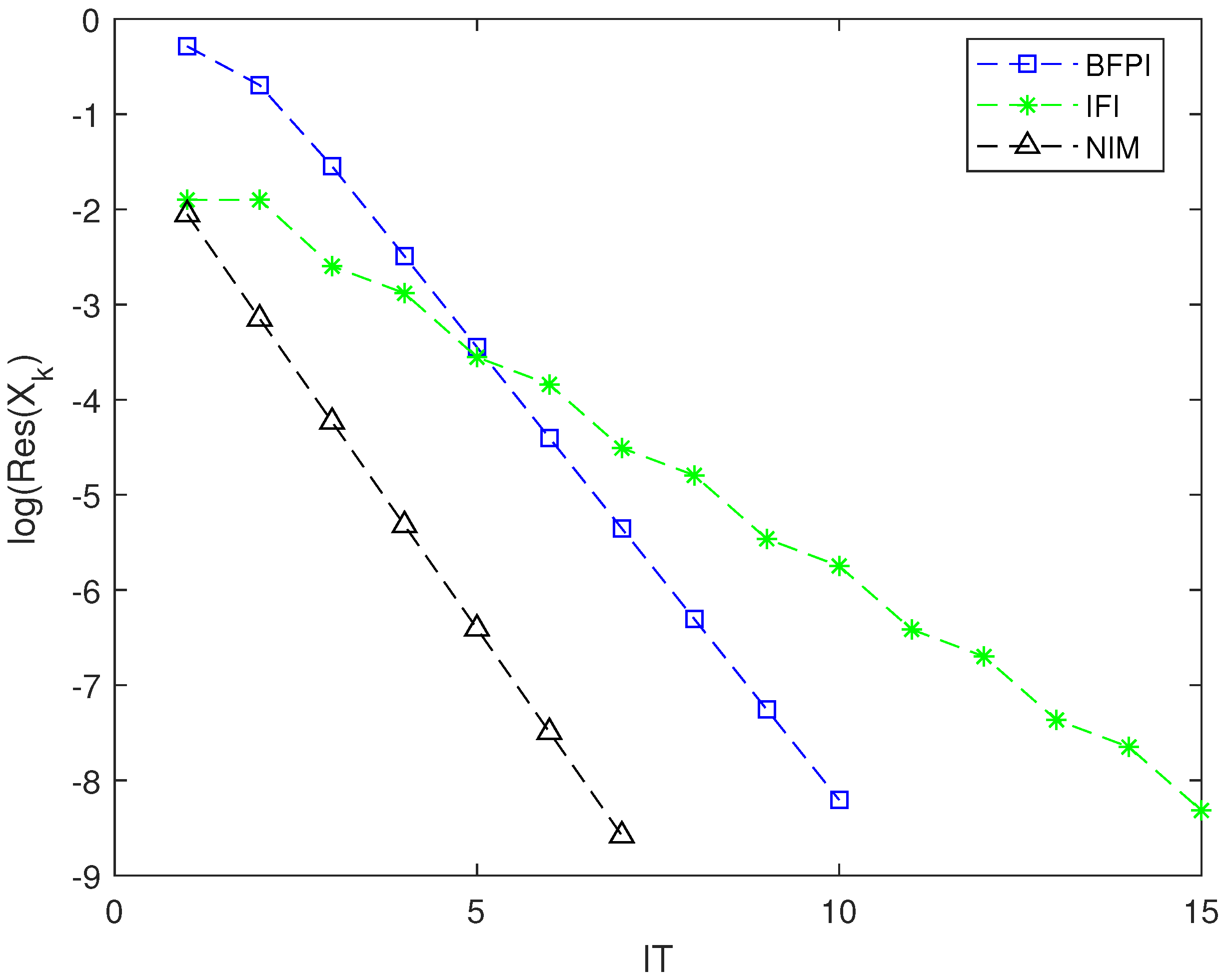
Numerical results for Example 1 are reported in Table 1 and Figure 1, which show that the BFPI costs the least computing time, but Newton’s iteration method obtains the highest accuracy and the fastest convergence speed among the three methods.

Table 1. The numerical results of Example 1.

Method	IT	CPU	Res $\left({\mathit{X}}_{\mathit{k}}\right)$
BFPI	10	0.003025	6.2142 × 10${}^{-9}$
IFI	15	0.004163	4.8205 × 10${}^{-9}$
NIM	7	0.018660	2.6335 × 10${}^{-9}$

Figure 1. The convergence process of the three iterations for computing Equation (1) for Example 1.

Example 2. 

Consider Equation (1) with

$$A_1=\frac{1}{550}\left(\begin{array}{cccccc}30& 22& 23& 35& 40& 52\\ 22& 17& 19& 66& 30& 10\\ 23& 19& 11& 13& 25& 21\\ 35& 66& 13& 19& 17& 6\\ 40& 30& 25& 7& 20& 15\\ 52& 10& 21& 6& 15& 9\end{array}\right),$$

$$A_2=\frac{1}{550}\left(\begin{array}{cccccc}11& 12& 15& 17& 20& 45\\ 12& 7& 19& 21& 51& 13\\ 15& 19& 65& 44& 23& 18\\ 17& 21& 44& 31& 32& 33\\ 20& 51& 23& 32& 13& 41\\ 45& 19& 18& 33& 41& 2\end{array}\right).$$

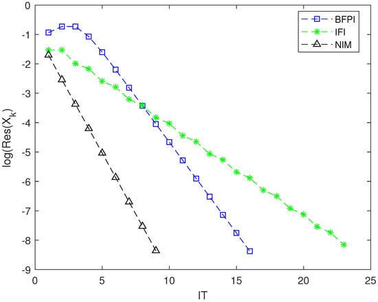
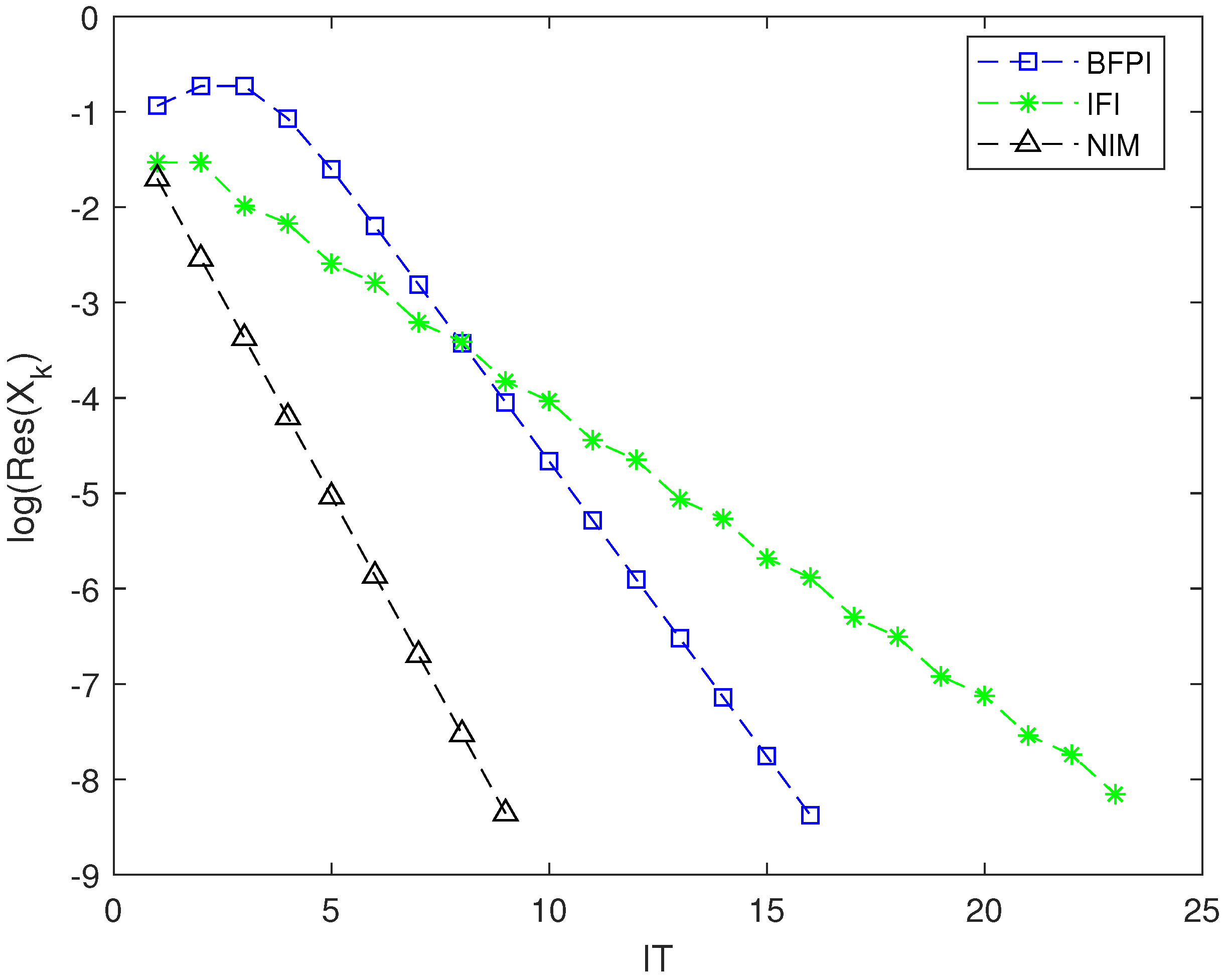
Table 2 reports the numerical results of Example 2. It reveals that the Newton iteration costs almost the same computing time as BFPI and achieves almost the same accuracy as BFPI; however, Figure 2 shows Newton’s iteration method converges the fastest among the three methods.

Table 2. The numerical results of Example 2.

Method	IT	CPU	Res $\left({\mathit{X}}_{\mathit{k}}\right)$
BFPI	16	0.003165	4.1922 × 10${}^{-9}$
IFI	23	0.005886	6.9625 × 10${}^{-9}$
NIM	9	0.004179	4.3841 × 10${}^{-9}$

Figure 2. The convergence process of the three iterations for computing Equation (1) for Example 2.

In addition, we specify the computational complexity of (6) in terms of matrix–matrix products and compare it with existing methods in the literature. See Table 3.

Table 3. The computational complexity of BFPI, IFI, and NIM.

Method	Computational Complexity
BFPI	$\frac{13m{n}^3}{3}$
IFI	$(4m+4)n^3$
NIM	$(2m+\frac{29}{3})n^3$

5. Conclusions

In this paper, based on Newton’s iteration method, and the Fréchet derivative technique, we give a sufficient condition for the existence of the HPD solution of Equation (1). Moreover, we prove that the matrix sequence generated by Newton’s iteration method converges to the unique HPD solution of this equation under some mild conditions. Finally, we obtain error estimates and convergence of the approximate HPD solutions to Equation (1). Numerical results show that the BFPI costs the least computing time, the computational complexity of Newton’s iteration method is the highest, but Newton’s iteration method obtains the highest accuracy and the fastest convergence speed among the three methods.

References

- Green, W.L.; Kamen, E.W. Stabilizability of linear systems over a commutative normed algebra with applications to spatially-distributed and parameter-dependent systems. SIAM J. Control Optim. 1985, 23, 1–18. [Google Scholar] [CrossRef] [Scilit]
- Anderson, W.N.; Morley, T.D.; Trapp, G.E. Ladder networks, fixpoints, and the geometric mean. Circuits Syst. Signal Process. 1983, 2, 259–268. [Google Scholar] [CrossRef] [Scilit]
- Pusz, W.; Woronowicz, S.L. Functional calculus for sesquilinear forms and the purification map. Rep. Math. Phys. 1975, 8, 159–170. [Google Scholar] [CrossRef] [Scilit]
- Anderson, W.N.; Kleindorfer, G.B.; Kleindorfer, P.R.; Woodroofe, M.B. Consistent estimates of the parameters of a linear system. Ann. Math. Stat. 1969, 40, 2064–2075. [Google Scholar] [CrossRef] [Scilit]
- Ouellette, D.V. Schur complements and statistics. Linear Alg. Appl. 1981, 36, 187–295. [Google Scholar] [CrossRef] [Scilit]
- Erfanifar, R.; Sayevand, K.; Esmaeili, H. A novel iterative method for the solution of a nonlinear matrix equation. Appl. Numer. Math. 2020, 153, 503–518. [Google Scholar] [CrossRef] [Scilit]
- Meini, B. Efficient computation of the extreme solutions of X + A*X−1A = Q and X − A*X−1A = Q. Math. Comput. 2001, 71, 1189–1204. [Google Scholar] [CrossRef] [Scilit]
- Engwerda, J.C.; Ran, A.C.M.; Rijkeboer, A.L. Necessary and sufficient conditions for the existence of a positive definite solution of the matrix equation X + A*X−1A = Q. Linear Alg. Appl. 1993, 186, 255–275. [Google Scholar] [CrossRef] [Scilit]
- Guo, C.H.; Lancaster, P. Iterative solution of two matrix equations. Math. Comput. 1999, 68, 1589–1603. [Google Scholar] [CrossRef] [Scilit]
- Ding, F.; Chen, T. On iterative solutions of general coupled matrix equations. SIAM J. Control Optim. 2006, 44, 2269–2284. [Google Scholar] [CrossRef] [Scilit]
- Caliò, F.; Garralda-Guillem, A.I.; Marchetti, E.; Galán, M.R. Numerical approaches for systems of Volterra–Fredholm integral equations. Appl. Math. Comput. 2013, 225, 811–821. [Google Scholar] [CrossRef] [Scilit]
- Marino, G.; Xu, H.K. A general iterative method for nonexpansive mappings in Hilbert spaces. J. Math. Anal. Appl. 2006, 318, 43–52. [Google Scholar] [CrossRef] [Scilit]
- Li, C.H.; Tam, P.K.S. An iterative algorithm for minimum cross entropy thresholding. Pattern Recognit. Lett. 1998, 19, 771–776. [Google Scholar] [CrossRef] [Scilit]
- Fital, S.; Guo, C.H. A note on the fixed-point iteration for the matrix equations X ± A*X−1A = I. Linear Alg. Appl. 2008, 429, 2098–2112. [Google Scholar] [CrossRef] [Scilit]
- Ullah, M.Z. A new inversion-free iterative scheme to compute maximal and minimal solutions of a nonlinear matrix equation. Mathematics 2021, 9, 2994. [Google Scholar]
- Zhang, H. Quasi gradient-based inversion-free iterative algorithm for solving a class of the nonlinear matrix equations. Linear Alg. Appl. 2019, 77, 1233–1244. [Google Scholar]
- Zhang, H.M.; Ding, F. Iterative algorithms for X + ATX−1A = I by using the hierarchical identification principle. J. Frankl. Inst.-Eng. Appl. Math. 2016, 353, 1132–1146. [Google Scholar]
- Long, J.H.; Hu, X.Y.; Zhang, L. On the Hermitian positive definite solution of the nonlinear matrix equation X + A*X−1A + B*X−1B = I. B. Braz. Math. Soc. 2008, 39, 371–386. [Google Scholar] [CrossRef] [Scilit]
- Vaezzadeh, S.; Vaezpour, S.M.; Saadati, R.; Park, C. The iterative methods for solving nonlinear matrix equation X + A*X−1A + B*X−1B = Q. Adv. Differ. Equ. 2013, 2013, 229. [Google Scholar] [CrossRef] [Scilit]
- Sayevand, K.; Erfanifar, R.; Esmaeili, H. The maximal positive definite solution of the nonlinear matrix equation X + A*X−1A + B*X−1B = I. Math. Sci. 2022. [Google Scholar] [CrossRef] [Scilit]
- Hasanov, V.I.; Hakkaev, S.A. Convergence analysis of some iterative methods for a nonlinear matrix equation. Comput. Math. Appl. 2016, 72, 1164–1176. [Google Scholar] [CrossRef] [Scilit]
- Weng, P.C.Y. Solving two generalized nonlinear matrix equations. J. Appl. Math. Comput. 2021, 66, 543–559. [Google Scholar] [CrossRef] [Scilit]
- Huang, B.; Ma, C. Some iterative methods for the largest positive definite solution to a class of nonlinear matrix equation. Numer. Algorithms 2018, 79, 153–178. [Google Scholar] [CrossRef] [Scilit]
- Ortega, J.M.; Rheinboldt, W.C. Iterative Solution of Nonlinear Equations in Several Variables; SIAM: Philadelphia, PA, USA, 2000. [Google Scholar]
- Horn, R.A.; Johnson, C.R. Matrix Analysis, 2nd ed.; Cambridge University Press: New York, NY, USA, 2013. [Google Scholar]
- He, Y.M.; Long, J.H. On the Hermitian positive definite solution of the nonlinear matrix equation . Appl. Math. Comput. 2010, 216, 3480–3485. [Google Scholar]
Disclaimer/Publisher’s Note: The statements, opinions and data contained in all publications are solely those of the individual author(s) and contributor(s) and not of MDPI and/or the editor(s). MDPI and/or the editor(s) disclaim responsibility for any injury to people or property resulting from any ideas, methods, instructions or products referred to in the content. |
© 2023 by the authors. Licensee MDPI, Basel, Switzerland. This article is an open access article distributed under the terms and conditions of the Creative Commons Attribution (CC BY) license (https://creativecommons.org/licenses/by/4.0/).