Portfolio Construction: A Network Approach

Abstract

A key parameter when investing is Time Horizon. One of the biggest mistakes investors make is not aligning the timeline of their goals with their investment portfolio. In other words, time horizons determine the investment portfolio you should construct. We examine which portfolios are the best for long-term investing, short-term investing, and intraday trading. This study presents a novel approach for portfolio construction based on Network Science. We use daily returns of stocks that compose the Dow Jones Industrial Average (DJIA) for a 25-year period from 1998 to 2022. Stock networks are estimated from (i) Pearson correlation (undirected linear statistical correlations), as well as (ii) Transfer Entropy (directed non-linear causal relationships). Portfolios are constructed in two main ways: (a) only four stocks are selected, depending on their centrality, with Markowitz investing weights, or (b) all stocks are selected with centrality-based investing weights. Portfolio performance is evaluated in terms of the following indicators: return, risk (total and systematic), and risk-adjusted return (Sharpe ratio and Treynor ratio). Results are compared against two benchmarks: the index DJIA, and the Markowitz portfolio based on Modern Portfolio Theory. The key findings are as follows: (1) Peripheral portfolios of low centrality stocks based on Pearson correlation network are the best in the long-term, achieving an extremely high cumulative return of around 3000% as well as high risk-adjusted return; (2) Markowitz portfolio is the safest in the long-term, while on the contrary, central portfolios of high centrality stocks based on Pearson correlation network are the riskiest; (3) In times of crisis, no portfolio is always the best. However, portfolios based on Transfer Entropy network perform better in most of the crises; (4) Portfolios of all stocks selected with centrality-based investing weights outperform in both short-term investing and intraday trading. A stock brokerage company may utilize the above findings of our work to enhance its portfolio management services.

1. Introduction

The construction of the optimal portfolio is a complex task. It requires careful consideration of various factors, including return, risk, and diversification. The goal of investors is to achieve the desired balance between return and risk via optimal diversification [1,2]. More specifically, investors aim for the greatest possible returns with some acceptable risk or, conversely, lowest possible risk given a certain return. Markowitz [3,4] initially proposed a mean-variance mathematical model for portfolio construction, best known as “Modern Portfolio Theory” (MPT). Sharpe and others [5,6,7] developed a pricing model for assets under risk and uncertainty. Markowitz and Sharpe shared the Nobel Prize in Economics for their revolutionary work in 1990. However, adding multiple constraints and increasing dimensionality can make the problem computationally difficult in the context of MPT [8].

Representation is the key to understanding any phenomenon. New representations can help us solve problems we could not solve before. Networks are the mathematical language for describing interdependencies, and therefore they are the best-known method to represent complex phenomena [9,10]. A network can be described as a collection of points joined together by lines [9,11]. The points are usually called as “nodes” or “vertices” and the lines are usually called as “links” or “edges”. Due to their abstract nature and their simple graphical representation, networks offer a powerful way to effectively model complex social and economic systems, such as the global stock market. It is crucial to note that networks can effectively capture the high heterogeneity of the relationships between the nodes, incorporating, at the local level, the information of “who is interacting with whom, at what strength, when, and in what way” [11]. In this context, so-called Network Science offers a new mathematical modeling framework that consists of concepts, methodologies, and tools to study a fundamental question: “how are the structural features of a network related to the practical issues we care about?” [9]. As the topology of local interdependencies at the microscopic level can have a significant impact on the global behavior of the system at the macroscopic level, Network Science has already been applied in a wide range of social and economic problems [12,13]. More specifically, Network Science has already been applied to portfolio construction [14,15,16,17,18]. In this context, the financial assets (stocks, bonds, commodities, etc.) are the nodes, while the interdependencies among them are the links-edges, which are weighted by the corresponding statistical correlation or causal relationship.

In order to eliminate meaningless correlations-relationships in the network, it is a common practice to filter the network before any analysis. This filtering can be realized based on some of the following well-known techniques, namely: (1) Threshold, (2) Minimum Spanning Tree (MST), (3) Planar Maximally Filtered Graph (PMFG). Concerning the threshold technique, a threshold-value is set to filter-eliminate the weak correlations [19,20,21,22,23,24,25]. Concerning MST and PMFG techniques [14,26,27,28,29,30], the “most significant” subgraph of the original network is obtained. Although widely used, these filtering techniques have been criticized because valuable information can be lost. More specifically, MST and PMFG techniques require the transformation of original correlation weights into distance weights as well as the elimination of some edges. This procedure may result in significant information loss concerning the topological-structural characteristics of the original correlation network [19].

After applying some filtering techniques, the portfolio can be constructed based on Network Science. The most usual tool for portfolio construction is the centrality of the nodes [14,15,17,18], which evaluates the significance of a node based on its position in the network. In other words, centrality evaluates how “central” or “peripheral” the node is in the network. In Refs. [14,15] the assets-nodes that comprise the portfolio are selected based on some centrality index (topological criterion). After the selection of assets-nodes, the contribution of each asset to the portfolio (investment weights of the portfolio) is either optimized based on MPT (Markowitz weights) or assumed uniform (1/N).

In Ref. [14], it was found that portfolios that are composed of peripheral stocks of the network outperform other portfolios that are composed of central stocks. The portfolios were evaluated in terms of risk-adjusted returns (Sharpe ratio). Similar results were found in [15], supporting the notion that portfolios composed of peripheral stocks are the most profitable (in terms of Sharpe ratio) and well-diversified. Similar results were also found in [18], where portfolios composed of peripheral stocks had higher performance in terms of return and risk. In Ref. [16], the portfolio construction was based on the MST results from the correlation network of stocks that compose the Dow Jones Industrial Average (DJIA). It was found that the portfolio that was composed of the “leaves” of the MST had higher performance than the index DJIA itself, but lower performance compared to Markowitz portfolio based on MPT. The portfolios were evaluated in terms of return, risk, and risk-adjusted returns. In Ref. [17], a new method was proposed, called “ρ-dependent strategy”, that was defined as follows. If the correlation between the centrality of the nodes and their Sharpe ratio is below a suggested threshold at some period $t$, then the portfolio is composed of low centrality stocks. Otherwise, the portfolio is composed of high centrality stocks. Moreover, an interesting connection between MPT and stocks’ centrality was found. More specifically, it was found that a Markowitz portfolio tends to allocate higher investing weights to peripheral stocks [17].

A key parameter when investing is the Time Horizon. The investment time horizon is the period of time one expects to hold an investment. One of the biggest mistakes investors make is not aligning the timeline of their goals with their investment portfolio. In other words, time horizons determine the investment portfolio you should construct. That is because the length of the investment horizon significantly affects the portfolio risk [31]. Given that time and uncertainty are inevitably entangled with investment decisions, it is generally understood that a long-term horizon can handle higher risk and uncertainty because the market overall is expected to trend upwards, and therefore there is enough time to recover the possible losses. On the other hand, short-term investors usually do not want to take that much risk. Of course, we should mention here that this first approach is highly dependent on the dynamically changing social and economic environment. For example, as we recently experienced, unexpected events with high social and economic impact, such as the COVID-19 Pandemic or the Russian-Ukrainian War, may result in high financial market volatility in the global stock market [32], which may significantly influence the investment decisions. In other words, unexpected geopolitical events or natural disasters can cause sudden and significant increase of the financial market volatility in the global stock market, which may lead investors to shorten their investment time horizons and become more risk averse. We distinguish the following three cases, namely: long-term investing, short-term investing and intraday investing (trading). We shall address the following three research questions, concerning portfolios of stocks, which are constructed based on Network Science:

Question 1.

Which portfolios are the best for long-term investing?

Question 2.

Which portfolios are the best for short-term investing?

Question 3.

Which portfolios are the best for intraday trading?

The term “best”, as well as the time durations of long-term, short-term, and intraday investing, are specified in Section 2. More specifically, the rest of the paper is structured as follows. In Section 2, we present the dataset of stocks (Section 2.1), the several methods for portfolio construction based on Network Science (Section 2.2), the three different time horizons and the relevant indicators for evaluating the performance of portfolios (Section 2.3), and the indices for analyzing the structure of the stock correlation network (Section 2.4). In Section 3, we present the results concerning the performance of portfolios (Section 3.1) and the structure of the stock correlation network (Section 3.2). In Section 4, we discuss the results accordingly (Section 4.1 and Section 4.2). In Section 5, we summarize our findings highlighting their implications for investors with different investment time horizons.

2. Materials and Methods

We present below the dataset of stocks, the several methods for portfolio construction based on Network Science, the three different time horizons, and the relevant indicators for evaluating the performance of portfolios. We also present the indices for analyzing the structure of the stock correlation network.

2.1. Data

The source of the data is Yahoo Finance [33], which is a well-established, freely accessible financial database. The key advantage of Yahoo Finance is that no registration or API token is required to use it. In addition, the user has immediate access to large volumes of data. We retrieved the daily closing prices (adjusted for splits) of 26 large American companies (Table 1). More specifically, these are the 26 out of the 30 stocks that comprise the Dow Jones Industrial Average (DJIA) index (January 2023). Due to data availability, we exclude the following four stocks: Goldman Sachs (GS), Visa (V), Salesforce (CRM), and Dow Chemical (DOW). We also retrieved the daily closing prices (adjusted for splits) of the index itself, namely the Dow Jones Industrial Average (DJIA). The data cover a period of 25 years (from January 1998 to December 2022). Daily closing prices are the standard benchmark used by investors to evaluate the performance of stocks over time, because in this way the intraday noise is filtered out, allowing trends to be captured effectively. For portfolio construction, we use the daily returns, calculated by the following formula [14,16]:

$$r_t=\frac{p_t-p_{t-1}}{p_{t-1}}$$

where:

Table 1. Tickers and Names of the companies-stocks.

AAPL	Apple	JPM	JPMorgan Chase
AMGN	Amgen	KO	Coca-Cola
AXP	American Express	MCD	McDonald’s
BA	Boeing	MMM	3M
CAT	Caterpillar	MRK	Merck
CSCO	Cisco	MSFT	Microsoft
CVX	Chevron	NKE	Nike
DIS	Disney	PG	Procter & Gamble
HD	Home Depot	TRV	Travelers Companies Inc
HON	Honeywell	UNH	UnitedHealth
IBM	IBM	VZ	Verizon
INTC	INTC Intel	WBA	Walgreen
JNJ	Johnson & Johnson	WMT	Wal-Mart

$r_t$ is the daily return at time (day) $t$

$p_t$ is the closing price at time $t$

$p_{t-1}$ is the closing price at time $t-1$

2.2. Portfolio Construction

Several portfolio construction methods are presented in this subsection. More specifically, in Section 2.2.1, we present the rolling window on which our analysis is based. In Section 2.2.2, we present the estimation of the stock correlation network as well as the centralities of stocks-nodes. In Section 2.2.3, we present the several methods for the selection of stocks-nodes, which compose the relevant portfolios. In Section 2.2.4, we present the several approaches to portfolio investing weights.

2.2.1. Rolling Window

We use the constructed daily returns (1998–2022) based on a rolling window of two years, as illustrated in Table 2. More specifically, the first year is used to provide historical data to estimate the stock correlation network and construct the relevant portfolio. The second year is used to evaluate the performance of the portfolio. The rolling window advances one year at a time. As a result, we have 24 years available for evaluating the performance of portfolios (1999–2022, 6039 days). We note that short selling is out of the scope of this work.

Table 2. Rolling Window.

1998	1999	2000	…	2021	2022
Data	Evaluation
	Data	Evaluation
		…	…
				Data	Evaluation

2.2.2. Networks of Stocks and Their Centralities

In this paper, we estimate networks of $N=26$ stocks (Table 1). Stock networks consist of nodes representing stocks and links-edges representing the interdependencies among them. The links are weighted according to the corresponding statistical correlation (Pearson ${\rho }_{ij}$) or causal relationship (Transfer Entropy $T_{i\to j}$ [34]) between the time series of daily returns of stocks. Therefore, we obtain the $N\times N=26\times 26$ weight matrix $W=\left(w_{ij}\right)$.

For network weights estimated based on Pearson’s coefficient $\left(w_{ij}={\rho }_{ij}\right)$, the undirected statistical correlation between two stocks $i$ and $j$ is linear, taking values in the interval $\left[-1, 1\right]$. We remove the diagonal elements $w_{ii}$ of weight matrix $W$, which represent autocorrelations. Therefore, the resulting network is weighted, signed, and undirected with zero self-weights $w_{ii}=0$. We also eliminate the off-diagonal elements $w_{ij}$ of weight matrix $W$ with low values in the interval $\left[-0.1, 0.1\right]$, representing weak correlations. This is mathematically formulated as follows:

$$w_{ij}=⟦{\rho }_{ij}\notin \left[-0.1, 0.1\right]⟧·{\rho }_{ij}$$

where $⟦\mathrm{Q}⟧$ is the Iverson bracket [35] that converts Boolean values to numbers 0, 1:

$$⟦\mathrm{Q}⟧=\{\begin{array}{c}1,\mathrm{if}\mathrm{Q}\mathrm{is}\mathrm{True}\\ 0,\mathrm{if}\mathrm{Q}\mathrm{is}\mathrm{False}\end{array}$$

This “threshold technique” is widely used to filter correlation networks in order to reduce complexity and facilitate the analysis [19,20,21,22,23,24]. We investigated several different threshold values and we selected $10\%$ because, in this case, the results can be captured more clearly.

For the weighted-undirected network estimated based on Pearson’s coefficient, we calculate the following centralities [9,10,36,37,38,39,40,41] of nodes-stocks, namely:

• weighted degree centrality (“strength”)
• weighted eigenvector centrality (“eigen”)
• weighted efficiency—Latora closeness (“closeness”)

For calculating strength and eigen, we take the absolute values of the weight matrix $W$, namely $\left|w_{ij}\right|$. In this way, we overcome the rare and low-value negative Pearson correlations, which was found by focusing on the intensity of correlation rather than its sign. For calculating closeness, the Pearson correlation weights $w_{ij}$ taking values in $\left[-1, 1\right]$ are transformed to distance weights $d_{ij}$ taking values in $\left[0, 2\right]$ according to the following formula:

$$d_{ij}=\sqrt{2·\left(1-w_{ij}\right)}$$

This transformation of weights is widely used in correlation networks [30,42,43,44].

For network weights estimated based on Transfer Entropy $\left(w_{i\to j}=T_{i\to j}\right)$ [45,46], the directed causal relationship between two stocks $i$ and $j$ is non-linear, taking values in the interval $\left[0,+\infty \right)$. The diagonal elements $w_{i\leftrightarrow i}$ of weight matrix $W$ are zero. Therefore, the resulting network is positively weighted and directed with zero self-weights $w_{i\leftrightarrow i}=0$. Transfer Entropy is a widely used association measure in finance [47,48,49], biomedical research [50,51], and neuroscience [52,53], as well as other disciplines.

Transfer Entropy is biased for small samples [54]. Therefore, in this paper we use the so-called “Effective Transfer Entropy” [46,54], which was proposed in order to remove the bias resulting from the small sample size. As we use effective transfer entropy, there is no need to filter the resulting network with some threshold. For the discretization-binning of data (time series of daily returns), we follow the usual method based on the relevance of tails of distributions, which is widely used for financial data [46,47,49].

For the positively weighted-directed network estimated based on Transfer Entropy, we calculate the following centralities [9,10,36,37,38,39,40,41] of nodes-stocks, namely:

• in and out degree centrality (“in-degree” and “out-degree”) calculated on the corresponding unweighted-directed network. This network results from the Adjacency Matrix, which has binary values 0 and 1, indicating the absence or existence of causal relationships, correspondingly.
• in and out weighted degree centrality (“in-strength” and “out-strength”)
• in and out weighted eigenvector centrality (“in-eigen” and “out-eigen”)

We present, in Table 3, a brief point-to-point comparison between the two association measures that we use in this paper to estimate the networks of stocks, namely the Pearson correlation coefficient and Transfer Entropy. In addition, we present, in Table 4, the centralities of nodes-stocks that we calculate in each corresponding network.

Table 3. Pearson Correlation versus Transfer Entropy.

Pearson Correlation Network	Transfer Entropy Network
Statistical Correlation	Causal Relationship
Undirected	Directed
Linear	Non-Linear
$\mathrm{Signed}\mathrm{values}\mathrm{in}\mathrm{the}\mathrm{interval}\left[-1,1\right]$	$\mathrm{Positive}\mathrm{values}\mathrm{in}\mathrm{the}\mathrm{interval}\left[0,+\infty \right)$
Threshold is set to 10% $\mathrm{Elimination}\mathrm{of}\mathrm{weights}\mathrm{with}\mathrm{values}\mathrm{in}\left[-0.1,+0.1\right]$	No Threshold is applied, due to the use of “Effective Transfer Entropy”

Table 4. Centralities of Nodes-Stocks.

Pearson Correlation Network		Transfer Entropy Network
Undirected Network		Directed Network
Weight Matrix with elements $w_{ij}={\rho }_{ij}\in \left[-1, 1\right]$		Weight Matrix with elements $w_{i\to j}=T_{i\to j}\in \left[0,+\infty \right)$
Absolute Weight Matrix with positive elements $\left|w_{ij}\right|\in \left[0, 1\right]$	Weight Matrix of Distances defined as:  $d_{ij}=\sqrt{2·\left(1-w_{ij}\right)}$ with $d_{ij}\in \left[0,2\right]$	Adjacency Matrix with elements 0 or 1 defined as: $a_{i\to j}=⟦w_{i\to j}\ne 0⟧$	Weight Matrix with elements $w_{i\to j}=T_{i\to j}\in \left[0,+\infty \right)$
Weighted Degree Centrality (“strength”)		In Degree Centrality (“in-degree”) & Out Degree Centrality (“out-degree”)	In Weighted Degree Centrality (“in-strength”) & Out Weighted Degree Centrality (“out-strength”)
Weighted Eigenvector Centrality (“eigen”)			In Weighted Eigenvector Centrality (“in-eigen”) & Out Weighted Eigenvector Centrality (“out-eigen”)
	Weighted Efficiency Latora Closeness (“closeness”)

2.2.3. Selection of Stocks

Each portfolio is composed of some selected stocks. We examine the following two selection scenarios for selecting stocks:

• Selection 1: Only 4 out of 26 stocks under consideration (Table 1) are selected, based on some centrality criterion, as follows:

  ○

  The four top stocks (central) with highest centrality are selected (“top”)

  ○

  The four middle stocks with intermediate centrality are selected (“mid”)

  ○

  The four bottom stocks (peripheral) with lowest centrality are selected (“bot”)

• Selection 2: All 26 stocks under consideration (Table 1) are selected.

Concerning Selection 1, when sorting the 26 stocks in a descending order, with respect to some centrality criterion, the centrality values of the stocks may be less distinct for some positions. By selecting four stocks for each class (“top”, “mid”, “bot”), there is a “safe distance” of seven stocks between the classes, namely: (4)-7-(4)-7-(4). In this way, the centrality criterion is strongly present, and therefore the ordering “central—intermediate—peripheral” is meaningful. Of course, this discussion is highly dependent on the specific dataset under consideration as well as on the specific centrality criterion used. Concerning Selection 2, it takes the advantage of higher diversification, due to the selection of all 26 stocks examined. However, it was found that the advantage of higher diversification tends to diminish, after including a few dozen stocks in the portfolio [55,56,57,58].

2.2.4. Investing Weights

The selected stocks included in the portfolio have different investing weights. We examine the following two weighting scenarios for the investing weights:

• Weighting 1: Markowitz investing weights (MPT), which minimize the portfolio risk for a given return, namely: the return resulting from 1/N allocation [14].
• Weighting 2: Centrality-based investing weights, which allocate higher investing weights at peripheral nodes-stocks with lower centrality value. We model this relationship of “centrality-investment” with two ways:

  ○

  “Lin”: Investing weights $q_i^{Lin}$, which follow a linear relationship with the centrality $c_i$ of nodes-stocks included in the portfolio.

  ○

  “Quad”: Investing weights $q_i^{Quad}$, which follow a quadratic relationship with the centrality $c_i$ of nodes-stocks included in the portfolio.

In Table 5, we present the three different combinations, namely A, B, and C, examined in this paper, for selecting stocks (Selection 1 and Selection 2) and investing weights (Weighting 1 and Weighting 2).

Table 5. Selection of Stocks and corresponding Investing Weights.

		Investing Weights
		Weighting 1	Weighting 2
Selection of Stocks	Selection 1	Combination A	$-$
	Selection 2	Combination B	Combination C

“Lin”: The investing weights $q_i^{Lin}$ are defined as follows:

$$q_i^{Lin}=\{\begin{array}{l}\frac{1}{N}, when c_1=c_2=\cdots =c_N\\ \frac{1-c_i}{N-{{\displaystyle \sum }}_{i=1}^N{c}_i}, otherwise\end{array}$$

where:

$q_i^{Lin}$ is the “Lin” investing weight of node-stock $i$

$c_i$ is the relevant centrality value of node-stock $i$

$N=26$ is the number of all nodes-stocks of the network.

We note that the sum of all investing weights $q_i^{Lin}$ is equal to one, namely:

$$q_1^{Lin}+q_2^{Lin}+\cdots +q_N^{Lin}=1$$

The quadratic relationship is obtained easily by raising to the power of two the above constrain about the investing weights $q_i^{Lin}$, namely:

$${\left(q_1^{Lin}+q_2^{Lin}+\cdots +q_N^{Lin}\right)}^2=1^2\iff {\displaystyle \sum }_{i=1}^N{\left(q_i^{Lin}\right)}^2+2·{\displaystyle \sum }_{i\ne j}{q}_i^{Lin}·q_j^{Lin}=1\iff \frac{{{\displaystyle \sum }}_{i=1}^N{\left(q_i^{Lin}\right)}^2}{1-2·{{\displaystyle \sum }}_{i\ne j}{q}_i^{Lin}·q_j^{Lin}}=1$$

“Quad”: The investing weights $q_i^{Quad}$ are defined as follows:

$$q_i^{Quad}=\{\begin{array}{l}\frac{1}{N}, when c_1=c_2=\cdots =c_N\\ \frac{{\left(q_i^{Lin}\right)}^2}{1-2·{{\displaystyle \sum }}_{i\ne j}{q}_i^{Lin}·q_j^{Lin}}, otherwise\end{array}$$

where:

$q_i^{Quad}$ is the “Quad” investing weight of node-stock $i$

$c_i$ is the relevant centrality value of node-stock $i$

$N=26$ is the number of all nodes-stocks of the network.

2.3. Portfolio Performance

We present the three different time horizons (Section 2.3.1) for evaluating the portfolio performance, as well as the relevant portfolio performance indicators (Section 2.3.2).

2.3.1. Time Horizon for Portfolio Performance

The portfolio performance is evaluated based on three different time horizons, namely: long-term investing, short-term investing, and intraday investing (trading), specified as follows:

• Long-term investing (24 Years): Evaluation of portfolio performance for all 24-years, cumulatively
• Short-term investing (1 Year): Evaluation of portfolio performance for each year, separately
• Intraday trading (1 Day): Evaluation of portfolio performance for each day, separately

We use a time period of 24 years, which is one of the longest time periods found in the relevant literature. In this way, we can evaluate the portfolio performance not only in times of economic expansion (high economic activity and growth), but also in turbulent times of crises-economic recession. We present, in Table 6, some important events-crises that occurred in the time period under consideration.

Table 6. Important Events—Crises.

Year	Event
1998	Russian Financial Crisis
2001	9/11 Terrorist Attacks
2002	Stock Market Downturn of 2002
2008	Global Financial Crisis
2011	Downgrade of US Federal Government Credit Rating
2015	Chinese Stock Market Turbulence (Stock Market sell-off)
2020	COVID-19 Pandemic
2022	Russian-Ukrainian War

2.3.2. Indicators for Portfolio Performance

We evaluate 45 different portfolio methods, based on Network Science. We compare the results against two benchmarks, namely the index DJIA and the Markowitz portfolio based on MPT. The abbreviations of each portfolio, constructed based on some specific method, are presented in the Appendix A.

For long-term and short-term investing, all portfolios are evaluated in terms of the following performance indicators:

• Return [2]
• Risk

  ○

  Total Risk (Standard Deviation) [2]

  ○

  Systematic Risk (Beta coefficient) [5]

• Risk-adjusted return

  ○

  Sharpe Ratio (Adjusted Return to Total Risk) [59]

  ○

  Treynor Ratio (Adjusted Return to Systematic Risk) [60]

To calculate Sharpe ratio and Treynor ratio, we follow the usual practice [14,15,16,43,61], setting the risk-free rate equal to zero (rf = 0).

For intraday trading, all portfolios are evaluated in terms of Return only. That is because we have only one value for the daily return (not time series). Therefore, we calculate the following indicator: the percentage of days where the portfolio exceeds the return of each benchmark (index DJIA, Markowitz portfolio). All portfolio construction methods and performance indicators are summarized in Table 7.

Table 7. Summary of Portfolio Construction Methods and Portfolio Performance Indicators.

Data (2.1)	Daily Returns (adjusted for splits) from January 1998 to December 2022
Rolling Window (2.2.1)	Window of 2 years, rolling by one year at a time $\mathrm{First}\mathrm{year}\to$ Estimation of correlation network and portfolio construction $\mathrm{Sec}\mathrm{ond}\mathrm{year}\to$ Evaluation of Portfolio Performance
Nodes (2.2.2)	26 stocks from index Dow Jones Industrial Average (DJIA)
Network Construction (2.2.2)	Pearson Correlation					Transfer Entropy
Network Weights (2.2.2)	$\mathrm{Undirected}\mathrm{with}\mathrm{signed}\mathrm{values}\mathrm{in}\mathrm{the}\mathrm{interval}\left[-1, 1\right]$					$\mathrm{Directed}\mathrm{with}\mathrm{positive}\mathrm{values}\mathrm{in}\mathrm{the}\mathrm{interval}\left[0,+\infty \right)$
Selection of Stocks in the portfolio (2.2.3)	Index DJIA (Benchmark A)	Markowitz Portfolio based on MPT (Benchmark B)		Network Approach to Portfolio Construction
		26/26		26/26		4/26
				Selection of All Stocks with different centrality-based investing weights		Top 4 Highest Centrality		Middle 4 Middle Centrality	Bottom 4 Lowest Centrality
Investing Weights of the portfolio (2.2.4)		Markowitz Weights for all 26 stocks: Minimize Risk (SD)for a given Return, which results from 1/N allocation		$q_i^{Lin}$	$q_i^{Quad}$	Markowitz Weights for the 4 selected stocks		Markowitz Weights for the 4 selected stocks	Markowitz Weights for the 4 selected stocks
Investing Horizon for portfolio performance (2.3.1)	Long-term (24 Years)		Short-term (1 Year)				Intraday Trading (1 Day)
Indicators for portfolio performance (2.3.2)	Return	Risk				Risk-adjusted return
		Total Risk (SD)		Systematic Risk (Beta coefficient)		Sharpe Ratio (Adjusted Return to Total Risk)		Treynor Ratio (Adjusted Return to Systematic Risk)

2.4. Network Structure Indices

We examine the evolution of network structure, as a whole, in terms of two indices: density [9] and degree centralization [37] (Table 8). Degree centralization is related to vulnerability [62] and targeted controllability [63] of the network.

Table 8. Network Structure Indices.

Pearson Correlation Network		Transfer Entropy Network
Undirected Network		Directed Network
Weight Matrix with elements $w_{ij}={\rho }_{ij}\in \left[-1, 1\right]$		Weight Matrix with elements $w_{i\to j}=T_{i\to j}\in \left[0,+\infty \right)$
Adjacency Matrix with elements 0 or 1 defined as: $a_{ij}=⟦w_{ij}\ne 0⟧$	Absolute Weight Matrix with positive elements $\left|w_{ij}\right|\in \left[0, 1\right]$	Adjacency Matrix with elements 0 or 1 defined as: $a_{i\to j}=⟦w_{i\to j}\ne 0⟧$	Weight Matrix with elements $w_{i\to j}=T_{i\to j}\in \left[0,+\infty \right)$
Density	Weighted Density	Density	Weighted Density
Degree Centralization	Weighted Degree Centralization	Degree Centralization	Weighted Degree Centralization

3. Results

The results are presented as follows. In Section 3.1, we present the results for portfolio performance, depending on the time horizon, namely: long-term investing (Section 3.1.1), short-term investing (Section 3.1.2), and intraday trading (Section 3.1.3). Each portfolio performance is compared against two benchmarks: the index DJIA and the Markowitz portfolio based on MPT. The comparison is realized in terms of return, risk (total and systematic), and risk-adjusted return (Sharpe ratio and Treynor ratio). In Section 3.2, we present the results concerning the evolution of network structure over time. The results were obtained using the R programming language [64].

3.1. Results on Portfolio Performance

Each portfolio construction method examined remains unchanged over time, whereas the selection of stocks (Section 2.2.3) and/or the investing weights (Section 2.2.4) may change over time, due to the evolution of the stock correlation network (Section 2.2.1 and Section 2.2.2). We present below the portfolio performance for long-term investing (Section 3.1.1), short-term investing (Section 3.1.2), and intraday trading (Section 3.1.3). The portfolio performance is evaluated in terms of several indicators (Section 2.3.2), namely: return, risk (total and systematic), and risk-adjusted return (Sharpe ratio and Treynor ratio).

3.1.1. Results on Long-Term Investing

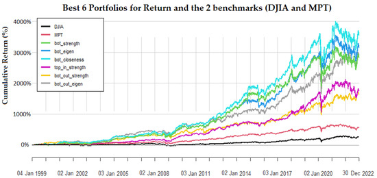
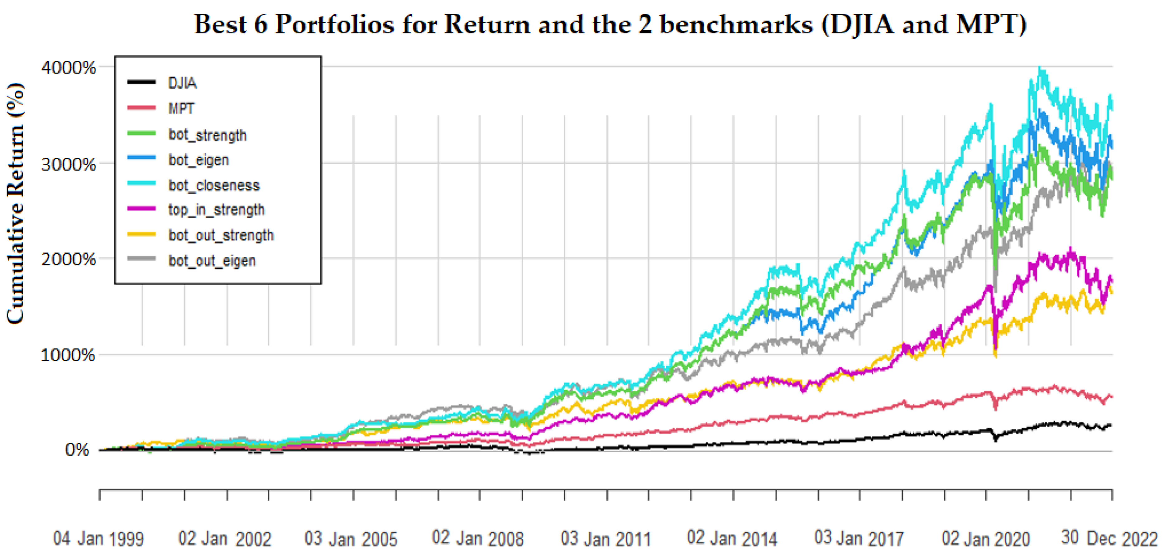
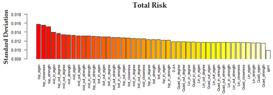
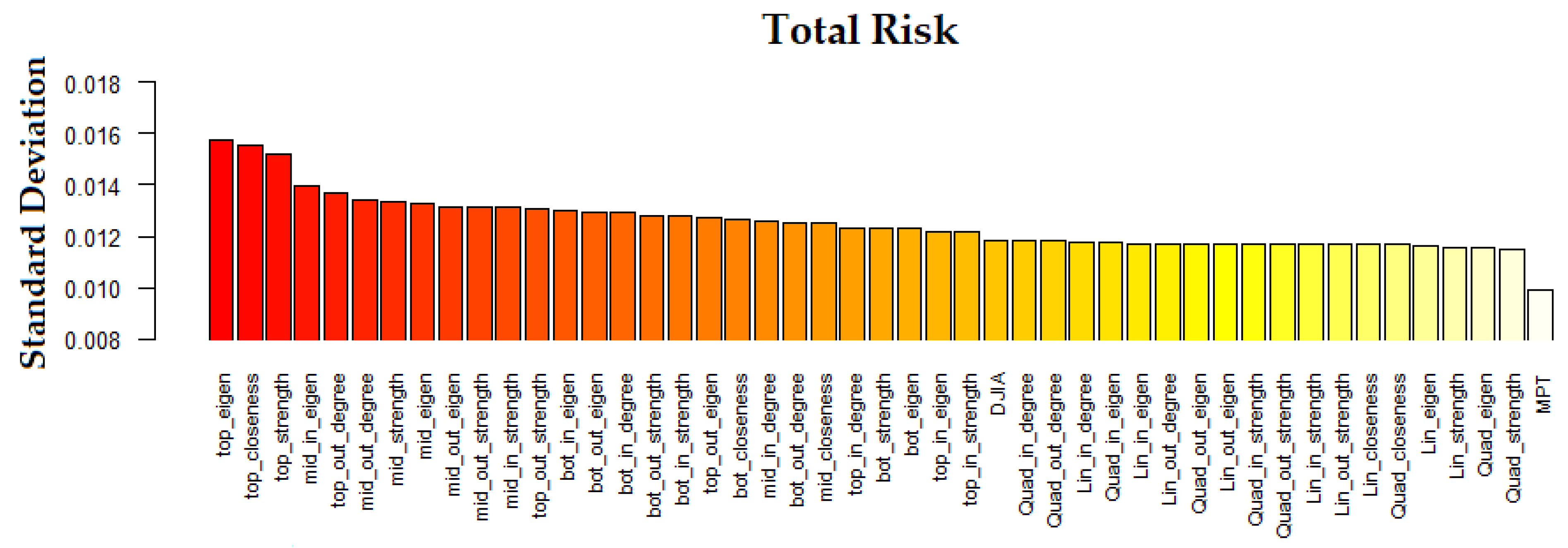
For long-term investing (24 years), we present indicative results for return (Figure 1), total risk (Figure 2), systematic risk (Figure 3), and risk-adjusted return (Sharpe ratio, Figure 4). All detailed results for long-term investing are provided in the Supplementary Materials (File S1).

Figure 1. Cumulative Return for long-term investing (24 years) of the best six portfolios as well as, the two benchmarks (“DJIA” and “MPT”). The interpretation of the different colors-labels is provided in the Appendix A.

Figure 2. Total Risk (Standard Deviation) for long-term investing (24 years) of all portfolios examined, including the two benchmarks (“DJIA” and “MPT”). The interpretation of the different labels is provided in Appendix A.

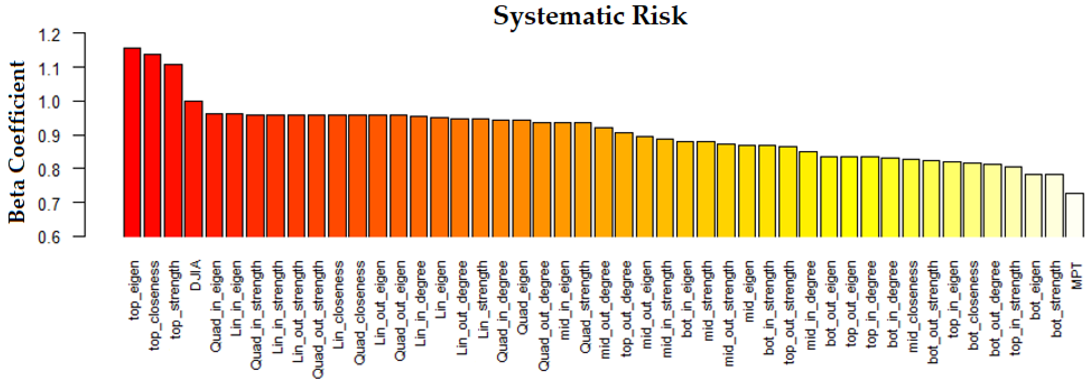
Figure 3. Systematic Risk (Beta Coefficient) for long-term investing (24 years) of all portfolios examined, including the two benchmarks (“DJIA” and “MPT”). The interpretation of the different labels is provided in Appendix A.

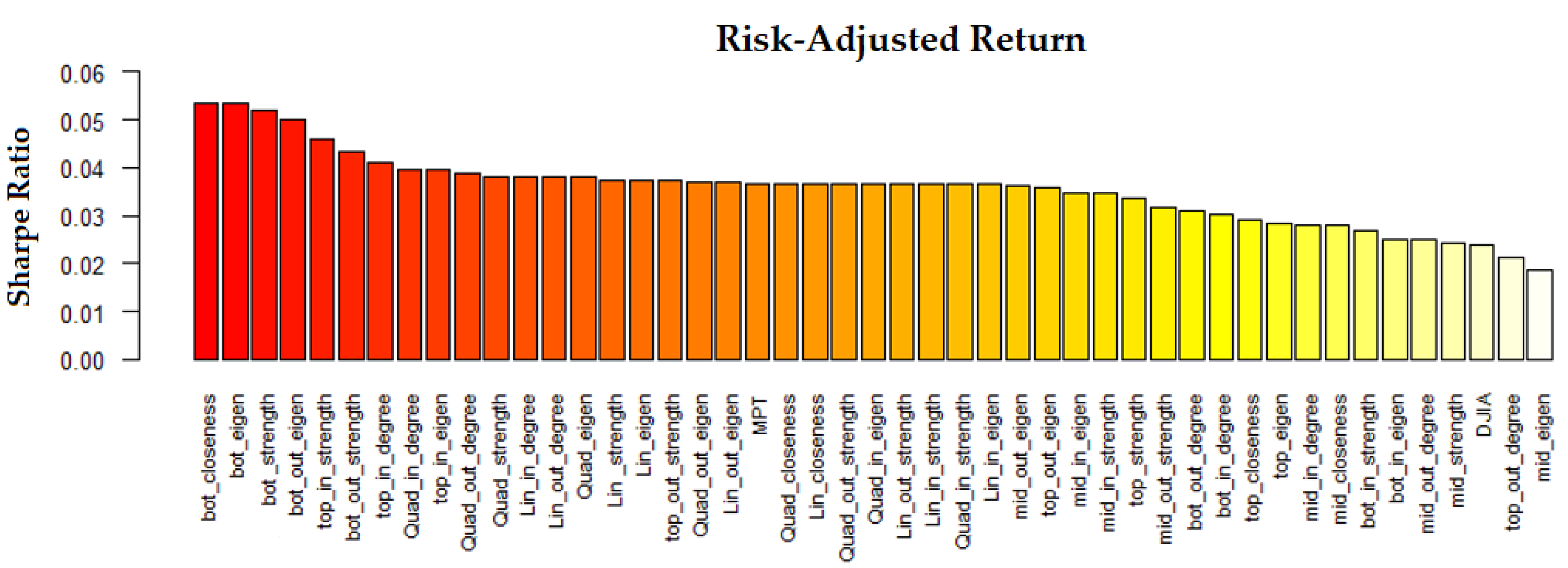
Figure 4. Risk-adjusted return (Sharpe Ratio) for long-term investing (24 years) of all portfolios examined, including the two benchmarks (“DJIA” and “MPT”). The interpretation of the different labels is provided in Appendix A.

3.1.2. Results on Short-Term Investing

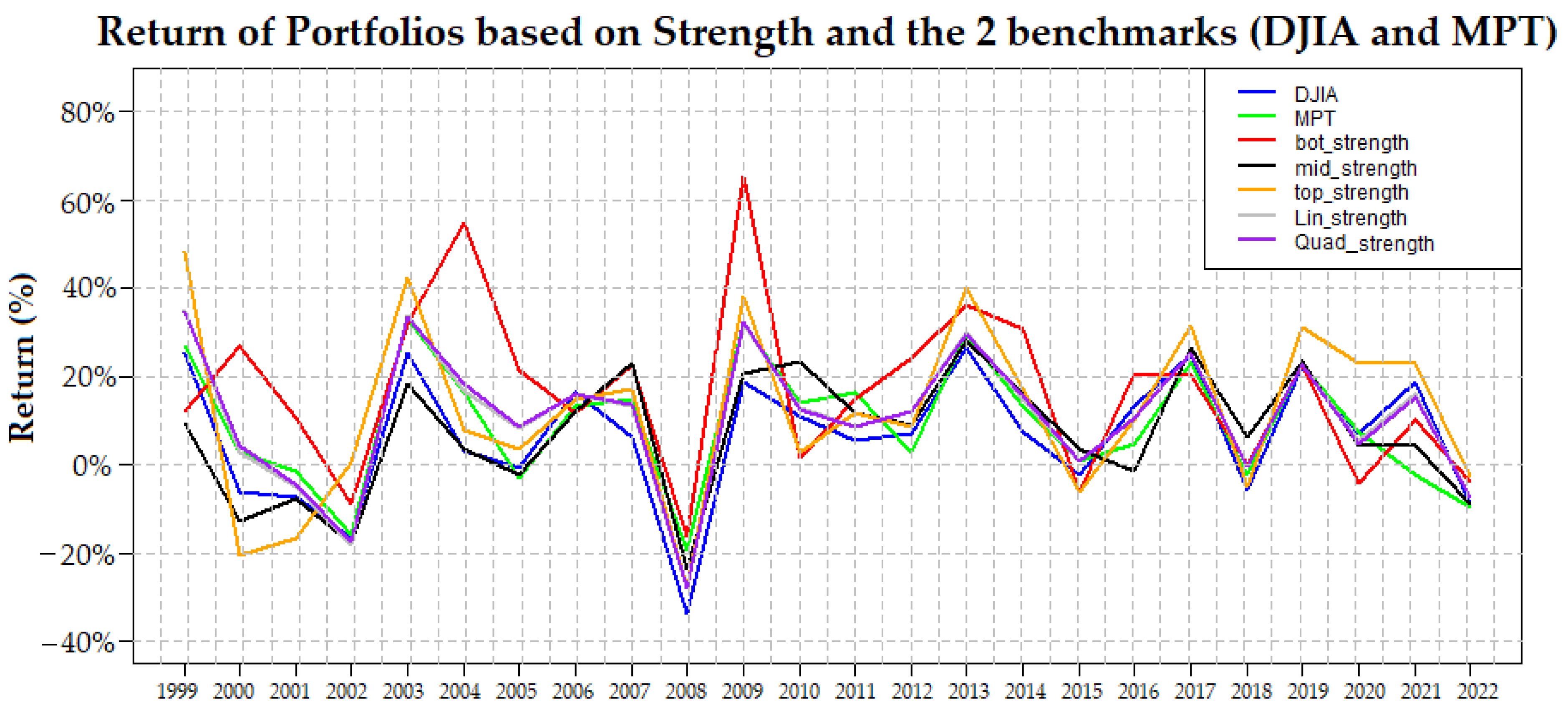
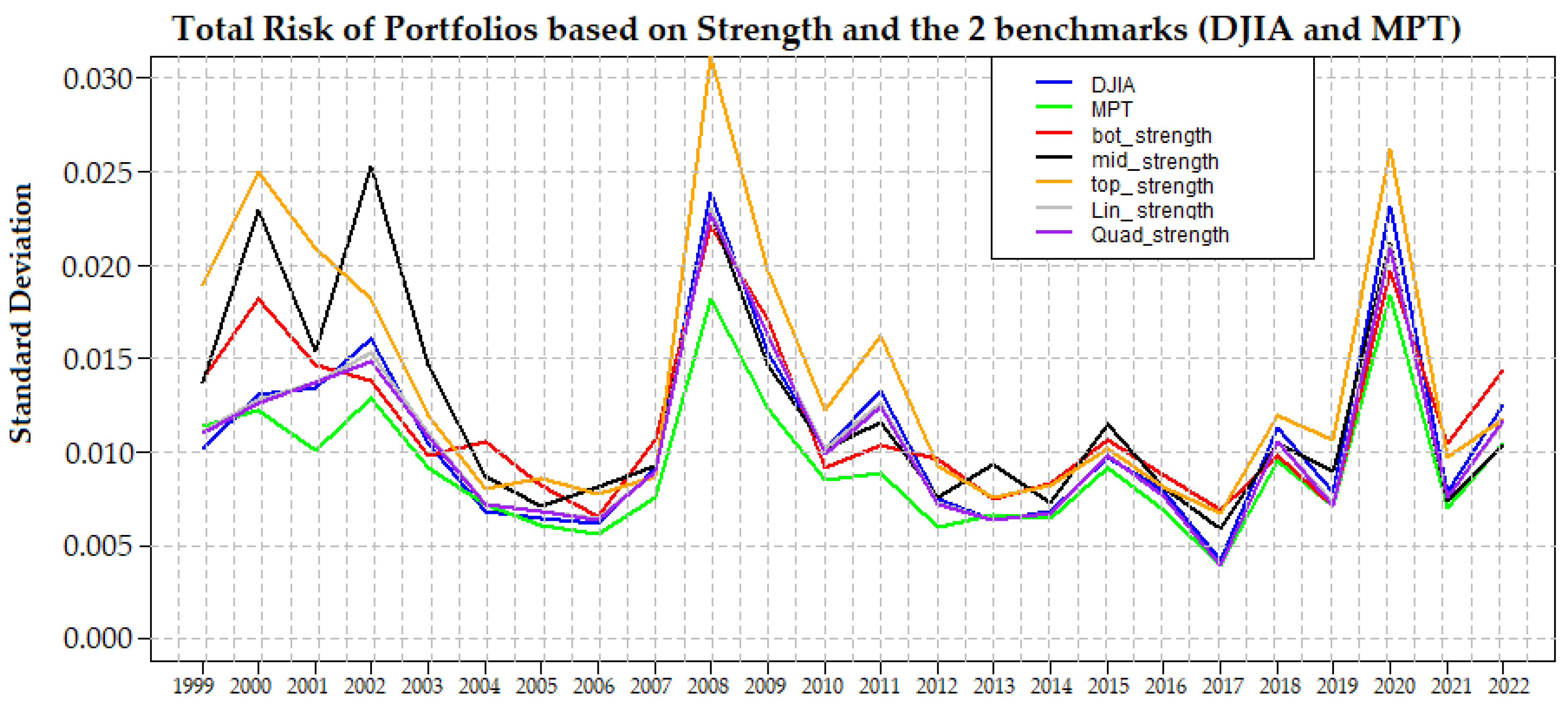
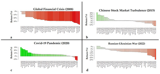
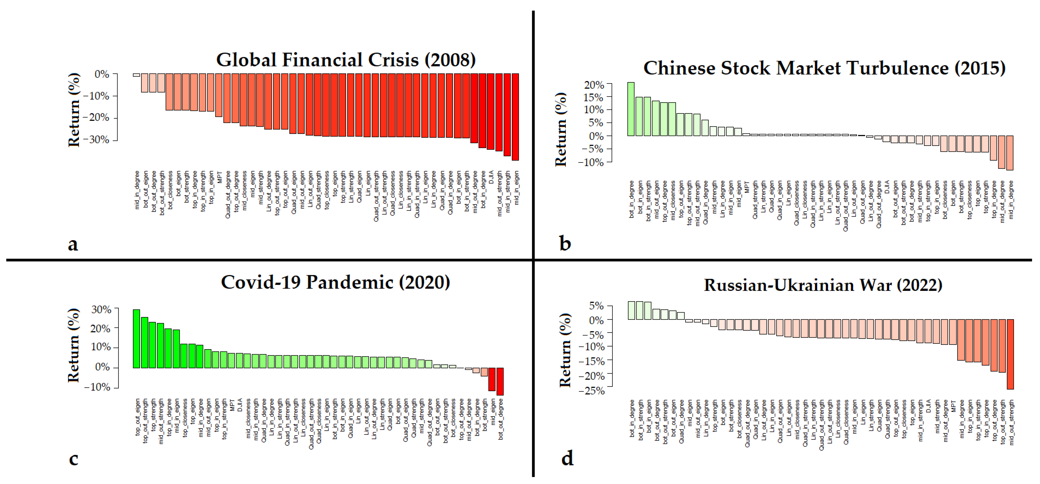
For short-term investing (1 year), we present indicative results for return (Figure 5), total risk (Figure 6), and systematic risk (Figure 7). We also present the difference of a portfolio’s return from DJIA’s return (Figure 8). In addition, we present the annual return of portfolios for four indicative crises with a strong impact on the global financial system (Figure 9). All detailed results for short-term investing are provided in the Supplementary Materials (File S2).

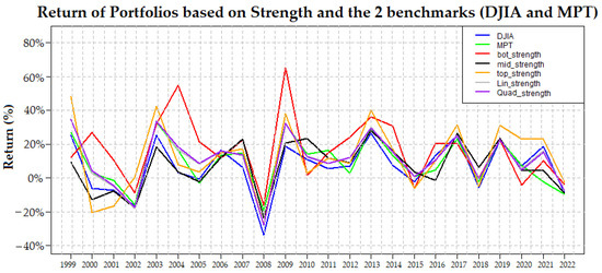
Figure 5. Return for short-term investing (1 year) of the five portfolios based on strength centrality, calculated on Pearson correlation networks, as well as the two benchmarks (“DJIA” and “MPT”). The interpretation of the different colors-labels is provided in Appendix A.

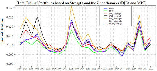
Figure 6. Total Risk (Standard Deviation) for short-term investing (1 year) of the five portfolios based on strength centrality, calculated on Pearson correlation networks, as well as the two benchmarks (“DJIA” and “MPT”). The interpretation of the different colors-labels is provided in Appendix A.

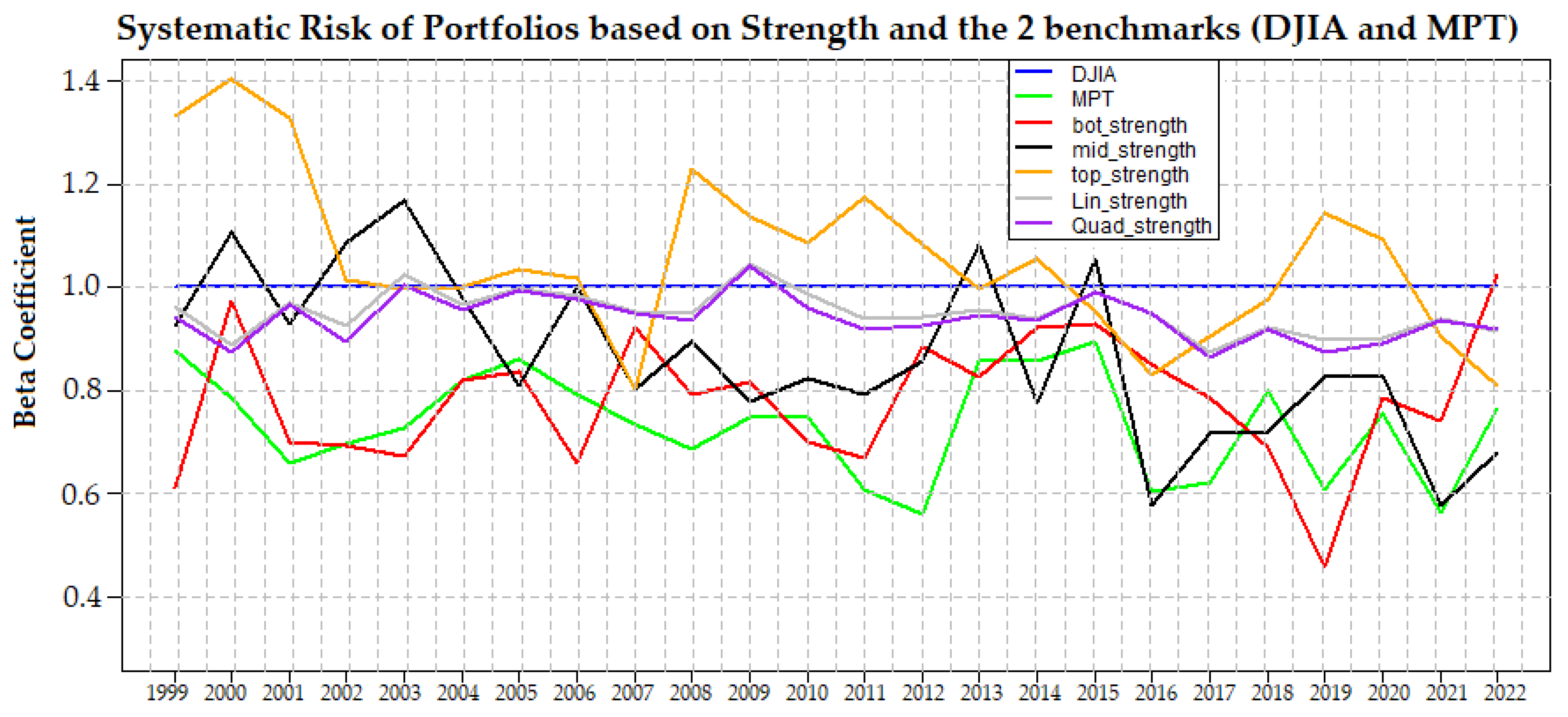
Figure 7. Systematic Risk (Beta Coefficient) for short-term investing (1 year) of the five portfolios based on strength centrality, calculated on Pearson correlation networks, as well as the two benchmarks (“DJIA” and “MPT”). The interpretation of the different colors-labels is provided in Appendix A.

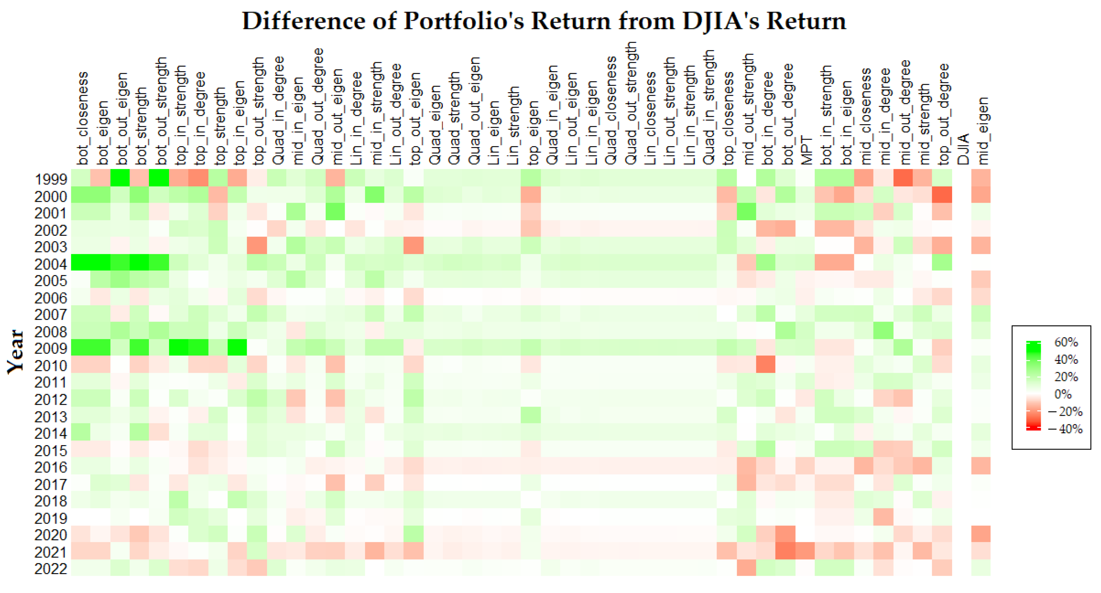
Figure 8. For short-term investing (1 year), we calculate the difference between the portfolio’s return with respect to DJIA’s return (reference rate). The interpretation of the different labels is provided in Appendix A.

Figure 9. Return for short-term investing (1 year) of all portfolios examined for four indicative crises with a strong impact on the global financial system. The interpretation of the different labels is provided in Appendix A.

3.1.3. Results on Intraday Trading

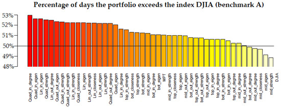
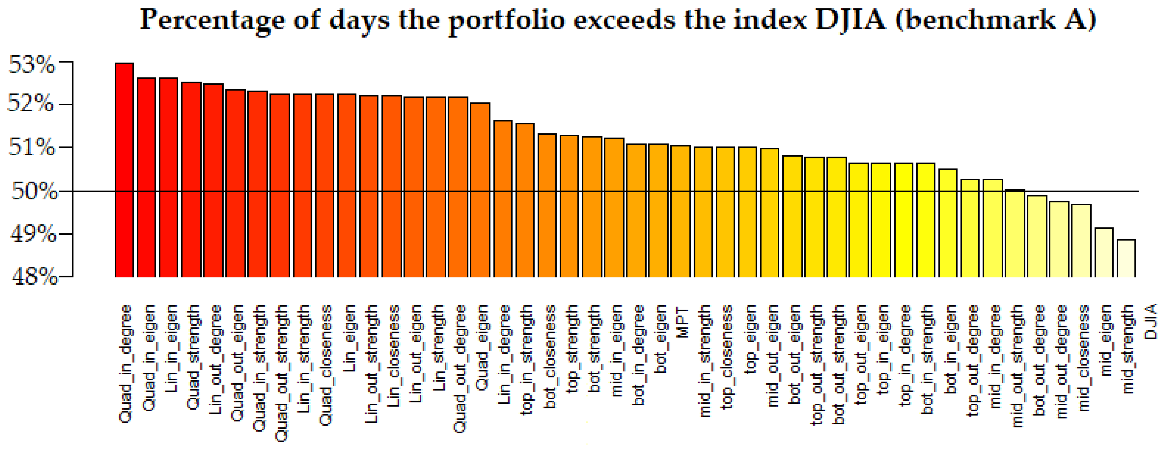
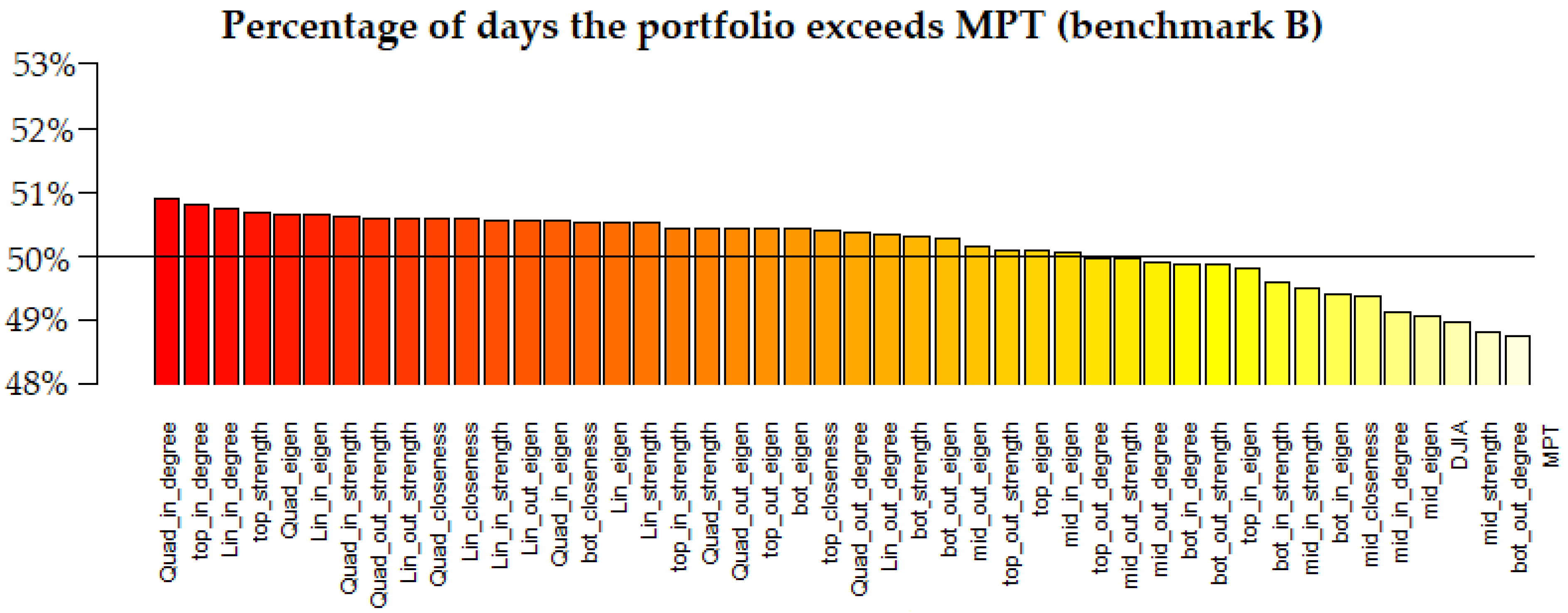
For intraday trading (1 day), we present the percentage of trading days the portfolio’s return exceeds the return of the two benchmarks, namely the index DJIA (Figure 10) and “MPT” portfolio (Figure 11).

Figure 10. The percentage of trading days in which the daily return of each portfolio exceeds the daily return of the index DJIA (benchmark A). The total number of trading days under consideration is 6039 (24 years). The interpretation of the different labels is provided in Appendix A.

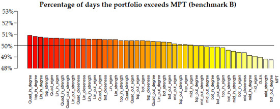
Figure 11. The percentage of trading days in which the daily return of each portfolio exceeds the daily return of “MPT” portfolio (benchmark B). The total number of trading days under consideration is 6039 (24 years). The interpretation of the different labels is provided in Appendix A.

3.2. Results on Network Structure

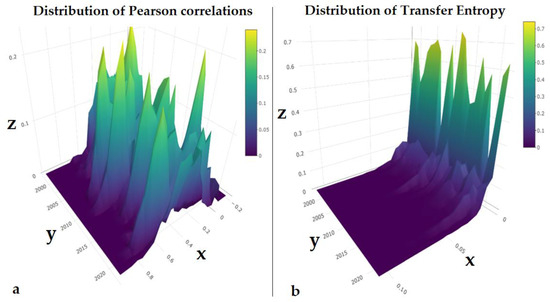
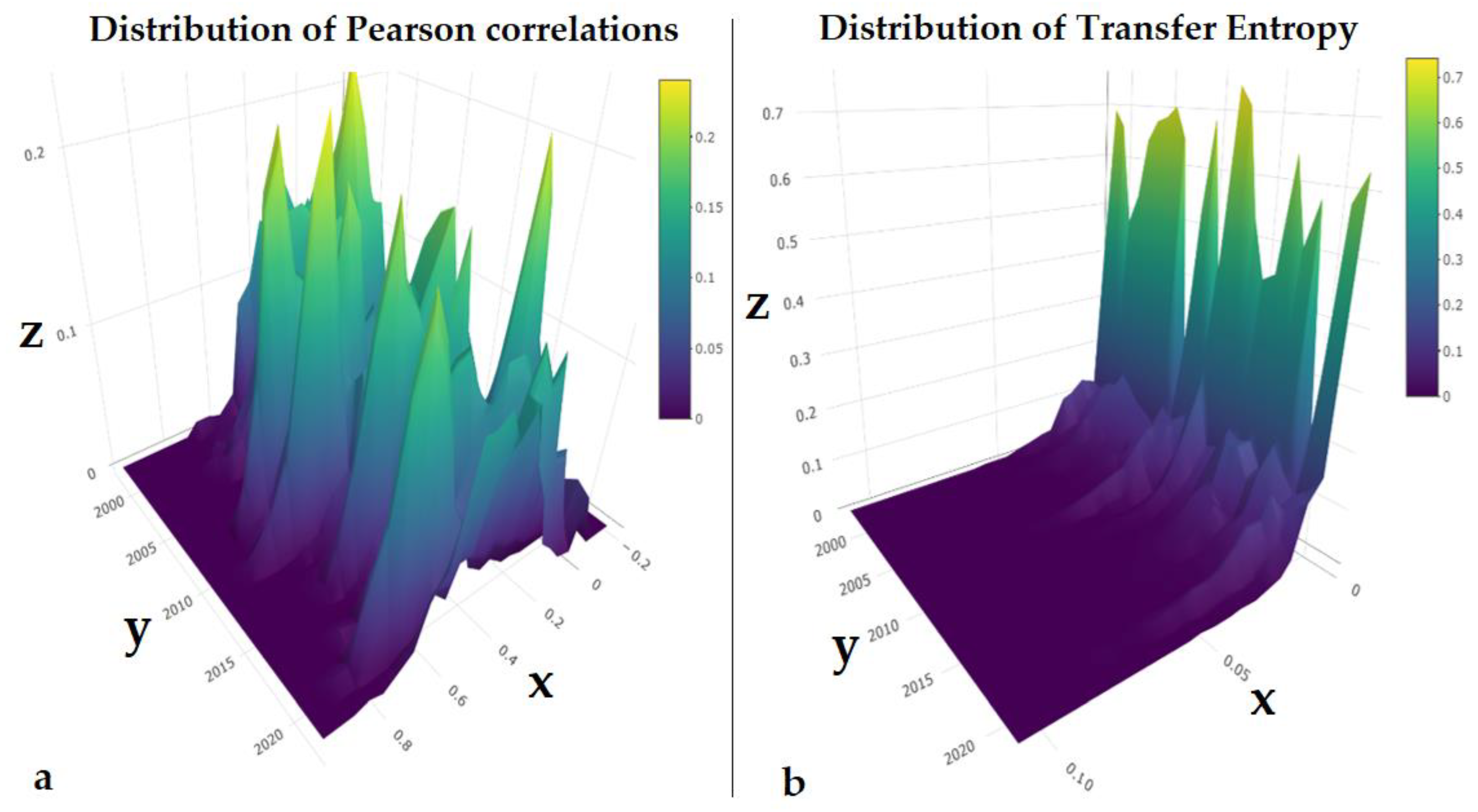
As portfolio construction is based on the centrality of nodes, the structure of the network is of utmost importance. Therefore, we examine the evolution of network structure, as a whole, in terms of density [9] and degree centralization [37]. As the results concerning density are the most interesting, we present them indicatively in the paper (Figure 12, Figure 13 and Figure 14). The detailed results for all network indices are provided in the Supplementary Materials (File S4). We also present the two empirical probability distributions of network weights for Pearson Correlation networks (Figure 15a) and Transfer Entropy networks (Figure 15b).

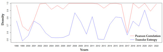
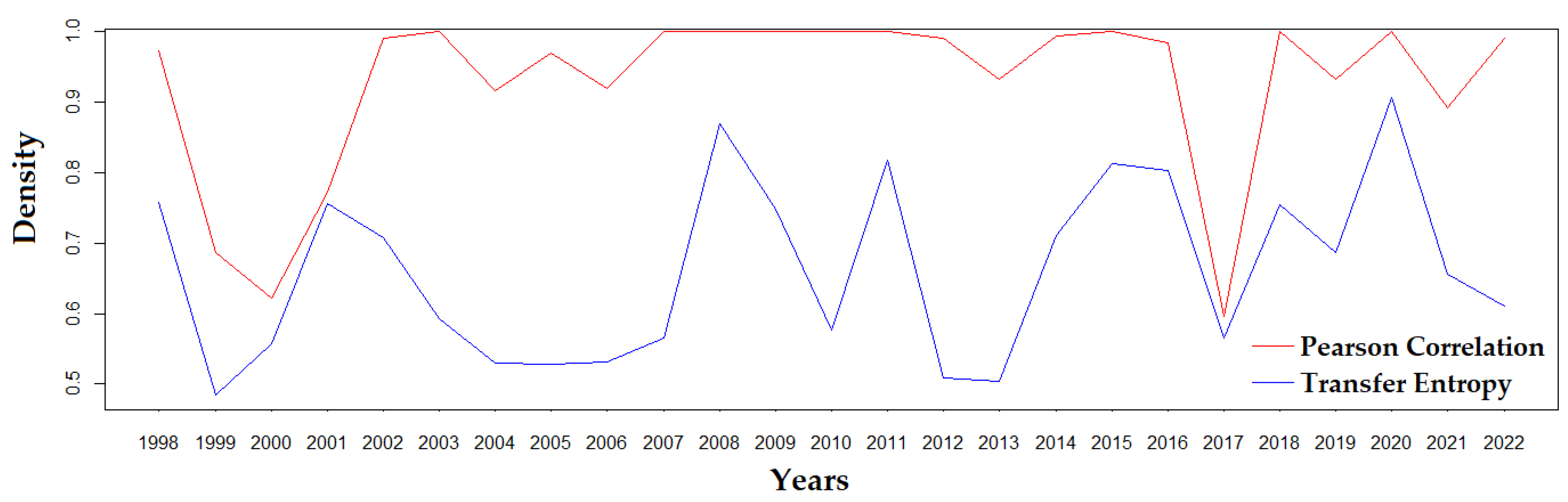
Figure 12. Density of the unweighted networks of stocks over time. The first network is estimated from Pearson correlation (red line). The second network is estimated from Transfer Entropy (blue line).

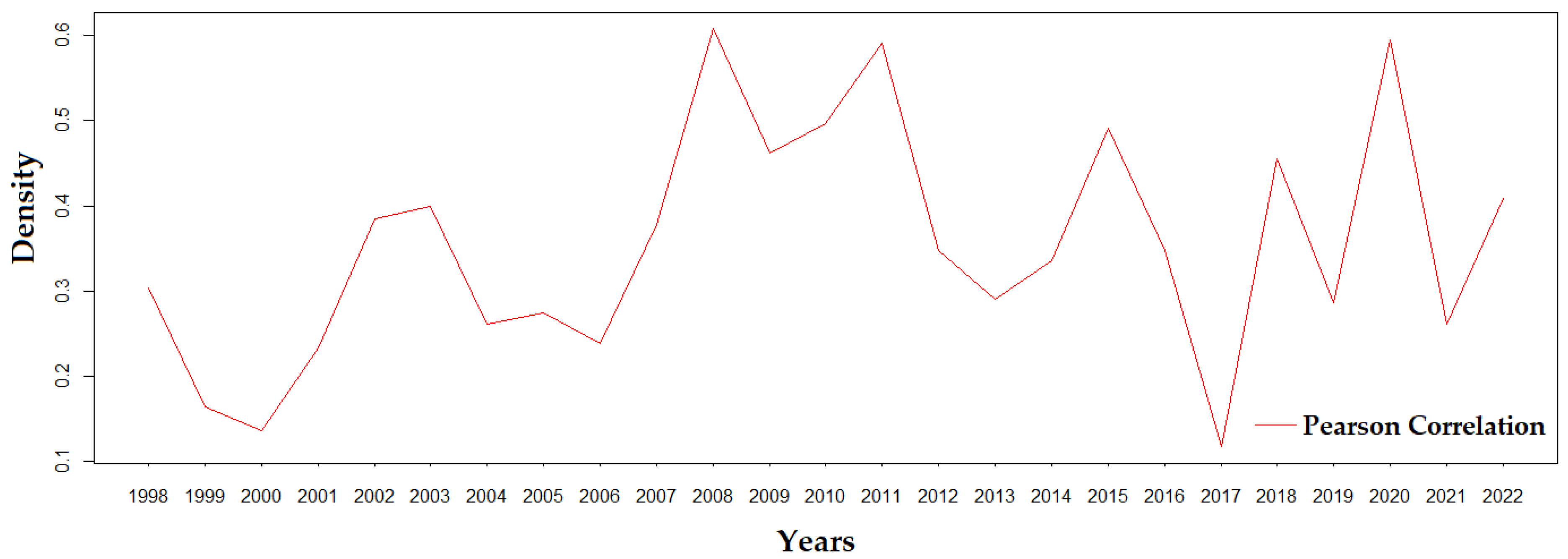
Figure 13. Density of the weighted network of stocks over time, estimated from Pearson correlation (red line).

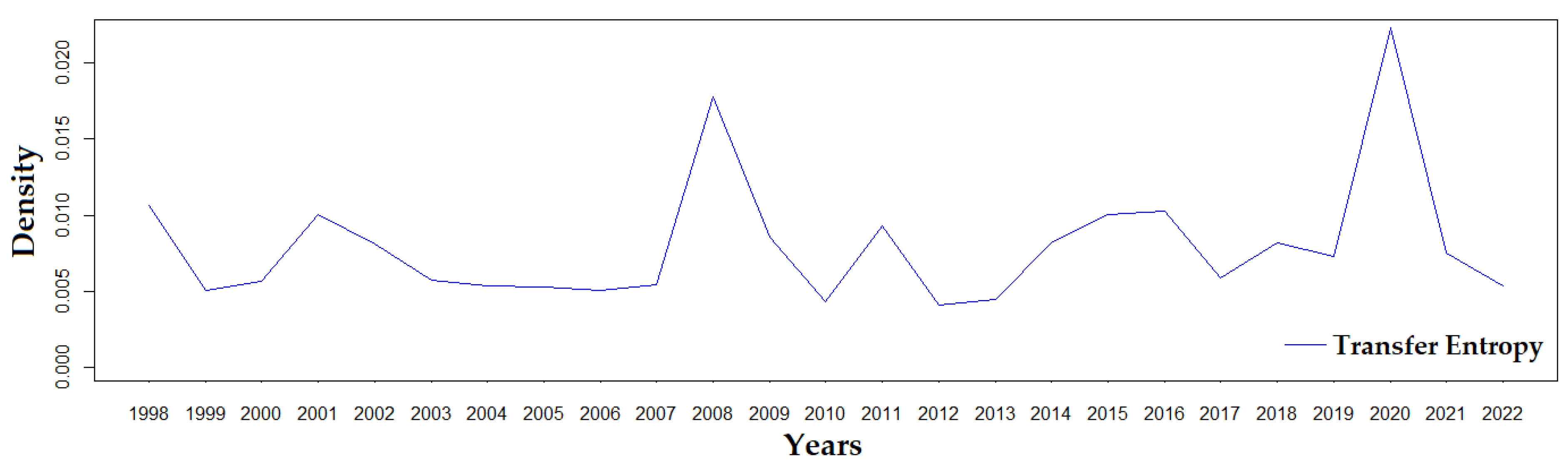
Figure 14. Density of the weighted network of stocks over time, estimated from Transfer Entropy (blue line).

Figure 15. Empirical Probability Distribution of Pearson correlations (x-axis) in relative frequency (z-axis) of the total weights for every year (y-axis) (a). Empirical Probability Distribution of Transfer Entropy (x-axis) in relative frequency (z-axis) of the total weights for every year (y-axis) (b).

4. Discussion

The discussion consists of seven remarks, summarizing the key points revealed from our analysis. More specifically, the discussion is structured as follows. In Section 4.1, we discuss the results of portfolio performance, depending on the time horizon, namely: long-term investing (Section 4.1.1), short-term investing (Section 4.1.2), and intraday trading (Section 4.1.3). In Section 4.2, we discuss the results concerning the evolution of network structure. We close the discussion highlighting the significance of our study (Section 4.3) and the areas for future research (Section 4.4).

4.1. Discussion on Portfolio Performance

4.1.1. Discussion on Long-Term Investing

Remark 1.

Peripheral portfolios based on Pearson correlation network are the best in the long-term.

Portfolios of peripheral (low centrality) stocks in the Pearson correlation network perform the best in the long-term, in terms of return and risk-adjusted return (Sharpe ratio and Treynor ratio). Strikingly, the three peripheral portfolios achieve superior performance, namely: “bot_strength”, “bot_eigen”, and “bot_closeness” (Appendix A). These three portfolios achieve an extremely high cumulative return of around 3000% (Figure 1) as well as high risk-adjusted return (Sharpe ratio in Figure 4, Treynor ratio in Supplementary Materials File S1) over the whole time period (1999–2022, 24 years). This finding may be understandable due to several factors, such as diversification, growth opportunities, and market disequilibrium [14]. It is worth mentioning that the index DJIA (benchmark A) achieves one of the lowest cumulative returns observed (around 260%) while “MPT” portfolio (benchmark B) achieves also a significantly low cumulative return (around 570%) (Figure 1, Supplementary Materials File S1). Generally speaking, the best performing portfolios in the long-term are based on Pearson correlation rather than Transfer Entropy network (Figure 1, Figure 2, Figure 3 and Figure 4, Supplementary Materials File S1). This finding may imply that long-term investing depends more on linear relationships than non-linear ones. This may be understandable, as, in the long-term, financial markets have less noise and therefore they are more predictable [65].

Remark 2.

Markowitz portfolio is the safest in the long-term, while, on the contrary, central portfolios based on Pearson correlation network are the riskiest.

The safest (less risky) portfolio in the long-term is the Markowitz portfolio based on “MPT” portfolio (benchmark B), in terms of total risk (Figure 2) and systematic risk (Figure 3). This is of course understandable because the Markowitz portfolio is constructed with the goal of minimizing total risk. On the contrary, portfolios of central (high centrality) stocks in the Pearson correlation network, namely “top_strength”, “top_eigen”, and “top_closeness” (Appendix A), are the riskiest in terms of total risk (Figure 2) and systematic risk (Figure 3).

4.1.2. Discussion on Short-Term Investing

Remark 3.

No portfolio is consistently the best in the short-term (on an annual basis).

No portfolio is consistently the best in the short-term. This finding holds for all performance indicators examined, namely return, risk (total and systematic), and risk-adjusted return (Sharpe ration and Treynor ratio). However, the following pattern can be detected: “Lin” and “Quad” portfolios follow closely and systematically the index DJIA (Figure 5, Figure 6 and Figure 7, Supplementary Materials File S2).

Remark 4.

“Lin” and “Quad” portfolios are slightly better than the index DJIA in the short-term (on annual basis), for most of the years under consideration.

“Lin” and “Quad” portfolios achieve slightly higher annual return (Figure 8) and lower systematic risk (Figure 7, Supplementary Materials File S2) compared to the index DJIA in the short-term for most of the years under consideration. For the rest, performance indicators (total risk, Sharpe ratio, Treynor ratio) “Lin” and “Quad” portfolios follow closely and systematically the index DJIA (Supplementary Materials File S2). The relatively low total risk of “Lin” and “Quad” portfolios, composed of all 26 stocks under consideration, is understandable due to their high diversification. The above findings suggest that “Lin” and “Quad” portfolios may be suitable for “passive investing” [66], as they follow the market (index DJIA) closely and systematically, without significant deviations.

Remark 5.

In times of crises, no portfolio is always the best. However, portfolios based on Transfer Entropy network perform better in most of the crises.

No portfolio is the best in all crises (Figure 9, Supplementary Materials File S2). However, portfolios based on Transfer Entropy network are usually better in times of crises. More specifically, in six out of seven crises, the best two portfolios are based on Transfer Entropy network (Supplementary Materials File S2). For the four crises presented in Figure 9, the best performing portfolio is always based on Transfer Entropy network. In the 2008 global financial crisis, the best four portfolios are based on Transfer Entropy network, having significantly lower losses compared to both benchmarks (“DJIA” and “MPT”) and other portfolios. The effectiveness of Transfer Entropy in times of crises is clearer in the 2015 and 2022 crises, where the “bot_in_degree” portfolio is the best with a remarkable return, while, on the contrary, the index DJIA (benchmark A) has losses.

The four crises presented in Figure 9 had strong impact on the global financial system. Concerning the global financial crisis of 2008, it is striking to observe that all portfolios have severe losses. Concerning the COVID-19 pandemic, although initially (2020Q1) all portfolios had severe losses (Figure 1), most of them rebounded rapidly in the same year, having eventually positive annual returns. Concerning the Chinese Stock Market Turbulence (2015) and the Russian-Ukrainian War (2022), it is interesting to note that the index DJIA (benchmark A) had losses, even though both crises originated outside the US. On the contrary, there are portfolios, mainly based on Transfer Entropy networks, with positive annual returns.

4.1.3. Discussion on Intraday Trading

Remark 6.

“Lin” and “Quad” portfolios have high probability (above 50%) to achieve higher daily return compared to both benchmarks (“DJIA” and “MPT”) in intraday trading.

“Lin” and “Quad” portfolios have above 50% probability to achieve higher daily return compared to both benchmarks (“DJIA” and “MPT”) in intraday trading (Figure 10 and Figure 11). In most cases, the “Lin” and “Quad” portfolios with high success rate against the two benchmarks, are based on Transfer Entropy. This expected up to a point, as 30 out of 45 portfolios examined are based on Transfer Entropy, while only 15 out of 45 portfolios are based on Pearson correlation. Concerning “Lin” and “Quad” portfolios, the top success rates against the index DJIA (52.96%, “Quad_in_degree”) and “MPT” portfolio (50.9%, “Quad_in_degree”) are slightly higher compared to similar analyses found in the relevant literature [16].

4.2. Discussion on Network Structure

Remark 7.

Network Density is increasing in times of crises. This behavior is captured more clearly in Transfer Entropy network.

In times of crisis, network density increases (Figure 12, Figure 13 and Figure 14); this is understandable because the massive sell-off in the stock market causes stocks to move in a correlated manner [67]. This finding is supported by the relevant literature [68,69,70]. More specifically, we found that network density is increasing due to two reasons, namely the increase of the number of links (unweighted network, Figure 12) and the increase of the value of weights (distribution of weights, Figure 15). The increase of weights’ values in times of crises, estimated by Pearson correlation, is supported by the relevant literature [30]. From the distribution of weights, we can also observe that negative correlations are rare and low, close to zero (Figure 15a). It is interesting to notice that Transfer Entropy is increasing more clearly compared to Pearson correlation in times of crisis (Figure 12, Figure 13 and Figure 14). This finding may imply that non-linear relationships dominate in times of crisis.

4.3. Significance of the Study—Comparison of the Key Findings with Respect to the Relevant Literature

The novelty of this paper is the evaluation of portfolio performance depending on the length of time horizon, namely (a) long-term investing, (b) short-term investing, and (c) intraday trading. This key point has not been addressed in the relevant literature to date by utilizing network science for portfolio construction. In addition, the main advantage of this work is the large period of time that we used (1998 to 2022). This fact allowed us to evaluate how the proposed methods for investing perform under a wide variety of different socioeconomic circumstances, including severe crises as well as periods of economic growth.

Our findings expand the existing knowledge about portfolio construction based on network science. We found that peripheral portfolios are the best in the long-term (Remark 1), while, on the contrary, central portfolios are the riskiest (Remark 2). Similar results have been reported in the relevant literature [14,15,17,18]. However, it is difficult to determine which portfolio is consistently the best for short-term investing (Remark 3). In fact, as the length of the investment time horizon shortens, the distinction between the different strategies for portfolio construction disappears [14,17]. By averaging the short-term performance of the portfolios, the result that has been reported in the relevant literature is that peripheral portfolios are better compared to central [14,16]. Our analysis revealed that the new models for investing weights based on centrality values, namely the “Lin” and “Quad” portfolios, are consistently better (even slightly) than the index DJIA for short-term investing (Remark 4). For intraday trading, “Lin” and “Quad” portfolios are better than both benchmarks (Remark 6).

Transfer entropy has been used for portfolio construction as an alternative way to estimate the correlation between stock market indices [47]. However, in the context of portfolio construction based on network science (using centralities), to the best of our knowledge, we are the first to compare the impact of different ways for estimating the stock correlation network. The result of this comparison is that portfolios based on Transfer Entropy network, rather than Pearson correlation network, perform better in most of the crises (Remark 5). In addition, another interesting pattern concerning crises is that network density is increasing, especially in Transfer Entropy network (Remark 7). This finding is supported by the relevant literature [30,68,69,70] and it is intuitively expected, because the massive sell-off in the stock market causes stocks to move in a correlated manner [67].

4.4. Limitations of the Study—Areas for Future Work

Regarding future work, a natural continuation of our work could be in the following three directions. First, instead of assigning investing weights based solely on the centrality of each node-asset, it is interesting to investigate investing weights based on the centrality as well as the Total Risk (Standard Deviation) and the Systematic Risk (Beta coefficient) of each node-asset itself. In this way, several risk factors are considered. Furthermore, one can consider other, more sophisticated centralities or even weighted combinations of different centralities with the aim of improving further the portfolio performance, especially during crises. Second, a network approach to portfolio construction can be applied to a wider (more diversified) spectrum of assets, including commodities, bonds, etc. In this case, the negative correlations of daily returns between the different assets may be stronger and more frequent, in contrast to our work, where negative Pearson correlations are rare and low value (Figure 15a). In such a case, the strong and frequent negative correlations between different kinds of assets can be utilized fruitfully to hedge risk. Investing into anti-correlated assets, called “hedge assets”, can be useful to offset potential losses [71,72,73,74,75]. Therefore, a promising future direction is to apply and extend the proposed network-based methodology for portfolio construction to signed and weighted correlation networks of assets, aiming to design optimal portfolios with desired balance between risk and return. Third, another interesting future work would be to integrate the proposed network approach to portfolio construction with the 3-factor [76] or 5-factor [77] model of Fama-French, which are both an extension of the original Capital Asset Pricing Model (CAPM).

5. Conclusions

In this paper, we propose a network approach to portfolio construction. We calculated daily returns of 26 DJIA’s stocks for a period of 25 years from 1998 to 2022. For each year, we estimate two networks, where the nodes represent the stocks and links-edges between them represent the interdependencies among them, weighted according to the corresponding statistical correlation (Pearson) or causal relationship (Transfer Entropy). We calculated several centrality indices on which we base the portfolio construction. We explored the following two methodologies. First, we select stocks based on their centrality, while the investing weights are determined by Modern Portfolio Theory. Second, all 26 stocks are included in the portfolio with investing weights according to their centrality. We evaluated the portfolios in terms of return, risk and risk adjusted return. The key novelty of this paper is that portfolio performance is evaluated with respect to different investment time horizons, namely: 24-years (long-term investing), one-year (short-term investing), and one day (intraday trading). The findings of this paper are summarized as follows:

Concerning long-term investing, we found that peripheral portfolios based on Pearson correlation network are the best in terms of return and risk-adjusted return (Remark 1). These portfolios achieve an extremely high cumulative return of around 3000% (Figure 1), much higher than the index DJIA (benchmark A), as well as high risk-adjusted return (Sharpe ratio in Figure 4, Treynor ratio in Supplementary Materials File S1). Markowitz portfolio (benchmark B) is the safest in the long-term, while on the contrary, central portfolios based on Pearson correlation network are the riskiest (Remark 2).

Concerning short-term investing, we conclude that no portfolio is consistently the best on an annual basis (Remark 3). Nevertheless, “Lin” and “Quad” portfolios are slightly better than the index DJIA on annual basis, for most of the years under consideration (Remark 4), as they achieve slightly higher annual return (Figure 8) and lower systematic risk (Figure 7, Supplementary Materials File S2).

Concerning intraday trading, “Lin” and “Quad” portfolios have high probability (above 50%) to achieve higher daily return compared to both benchmarks, namely the index DJIA and “MPT” portfolio (Figure 10 and Figure 11, Remark 6). From the above results, concerning short-term investing and intraday trading, we conclude that “Lin” and “Quad” portfolios are suitable for “passive investing” [66], as they closely follow the index DJIA consistently in time, producing even better outcomes.

Concerning portfolio performance in times of crisis (Table 6), we found that no portfolio was the best in all crisis. However, portfolios based on Transfer Entropy network performed better in most of the crises (Remark 5). It is worth mentioning that during crisis, network density is increasing (Figure 12, Figure 13 and Figure 14), especially when networks are estimated based on Transfer Entropy rather than Pearson correlation (Remark 7).

The above findings suggest the following: if the investor is willing to take a higher risk than the risk associated with the index DJIA, then the peripheral portfolios based on Pearson correlation are the most suitable with respect to risk-adjusted return. On the other hand, if the investor is risk averse, the “Lin” and “Quad” portfolios are the most suitable, because they have consistently higher returns than the index DJIA (even slightly) with lower systematic risk and high diversification.

The practical significance of this study lies in the innovative application of network science to portfolio construction. A stock brokerage company may utilize the findings of our work to enhance its portfolio management services. The proposed methods provide a fresh perspective on investment strategies, potentially leading to more efficient portfolio allocations. By understanding linear and non-linear relationships among stocks, the members of an investment committee can gain a more comprehensive view of market dynamics and correlations. An investment company can utilize the knowledge provided from this work to develop more customized and efficient investment models.

References

- Goetzman, W.N.; Brown, S.J.; Gruber, M.J.; Elton, E.J. Modern Portfolio Theory and Investment Analysis, 9th ed.; John Wiley & Sons: Hoboken, NJ, USA, 2014. [Google Scholar]
- Reilly, F.K.; Brown, K.C. Investment Analysis & Portfolio Management, 10th ed.; Cengage Learning: Boston, MA, USA, 2011. [Google Scholar]
- Markowitz, H. Portfolio Selection. J. Financ. 1952, 7, 77–91. [Google Scholar]
- Markowitz, H. Portfolio Selection: Efficient Diversification of Investments; Wiley: New York, NY, USA, 1959. [Google Scholar]
- Sharpe, W.F. Capital Asset Prices: A Theory of Market Equilibrium under Conditions of Risk. J. Financ. 1964, 19, 425–442. [Google Scholar]
- Lintner, J. Security Prices, Risk and Maximal Gains from Diversification. J. Financ. 1965, 20, 587–615. [Google Scholar]
- Mossin, J. Equilibrium in a Capital Asset Market. Econometrica 1966, 34, 768–783. [Google Scholar] [CrossRef] [Scilit]
- Masmoudi, M.; Abdelaziz, F.B. Portfolio selection problem: A review of deterministic and stochastic multiple objective programming models. Ann. Oper. Res. 2018, 267, 335–352. [Google Scholar] [CrossRef] [Scilit]
- Newman, M.J. Networks: An Introduction; Oxford University Press Inc.: New York, NY, USA, 2010. [Google Scholar]
- Caldarelli, G.; Vespignani, A. Large Scale Structure and Dynamics of Complex Networks: From Information Technology to Finance and Natural Science; World Scientific Publishing Co., Pte. Ltd.: Singapore, 2007. [Google Scholar]
- Thurner, S.; Hanel, R.; Klimek, P. Introduction to the Theory of Complex Systems; Oxford University Press: Oxford, UK, 2018. [Google Scholar]
- Jackson, M.O. Social and Economic Networks; Princeton University Press: Princeton, NJ, USA, 2010. [Google Scholar]
- Goyal, S. Networks an Economics Approach; The MIT Press: Cambridge, MA, USA, 2023. [Google Scholar]
- Pozzi, F.; Di Matteo, T.; Aste, T. Spread of risk across financial markets: Better to invest in the peripheries. Sci. Rep. 2013, 3, 1665. [Google Scholar] [CrossRef] [Scilit] [PubMed]
- Li, Y.; Jiang, X.-F.; Tian, Y.; Li, S.-P.; Zheng, B. Portfolio optimization based on network topology. Phys. A 2019, 515, 671–681. [Google Scholar] [CrossRef] [Scilit]
- Danko, J.; Soltes, V.; Bindzar, T. Portfolio Creation Using Graph Characteristics and Testing Its Performance. Montenegrin J. Econ. 2022, 18, 7–17. [Google Scholar] [CrossRef] [Scilit]
- Peralta, G.; Zareei, A. A network approach to portfolio selection. J. Empir. Financ. 2016, 38, 157–180. [Google Scholar] [CrossRef] [Scilit]
- Zhao, L.; Wang, G.-J.; Wang, M.; Bao, W.; Li, W.; Stanley, H.E. Stock market as temporal network. Phys. A 2018, 506, 1104–1112. [Google Scholar] [CrossRef] [Scilit]
- Tse, C.K.; Liu, J.; Lau, F.C. A network perspective of the stock market. J. Empir. Financ. 2010, 17, 659–667. [Google Scholar] [CrossRef] [Scilit]
- Moghadam, H.E.; Mohammadi, T.; Kashani, M.F.; Shakeri, A. Complex networks analysis in Iran stock market: The application of centrality. Phys. A Stat. Mech. Its Appl. 2019, 531, 121800. [Google Scholar] [CrossRef] [Scilit]
- Nobi, A.; Maeng, S.E.; Ha, G.G.; Lee, J.W. Effects of global financial crisis on network structure in a local stock market. Phys. A 2014, 407, 135–143. [Google Scholar] [CrossRef] [Scilit]
- Koldanov, A.P.; Koldanov, P.A.; Kalyagin, V.A.; Pardalos, P.M. Statistical procedures for the market graph construction. Comput. Stat. Data Anal. 2013, 68, 17–29. [Google Scholar] [CrossRef] [Scilit]
- Boginski, V.; Butenko, S.; Pardalos, P.M. Statistical analysis of financial networks. Comput. Stat. Data Anal. 2005, 48, 431–443. [Google Scholar] [CrossRef] [Scilit]
- Nobi, A.; Lee, S.; Kim, D.H.; Lee, J.W. Correlation and network topologies in global and local stock indices. Phys. Lett. A 2014, 378, 2482–2489. [Google Scholar] [CrossRef] [Scilit]
- Ioannidis, E.; Tsoumaris, D.; Ntemkas, D.; Sarikeisoglou, I. Correlations of ESG Ratings: A Signed Weighted Network Analysis. Appl. Math. 2022, 2, 638–658. [Google Scholar] [CrossRef] [Scilit]
- Tumminello, M.; Aste, T.; Di Matteo, T.; Mantegna, R.N. A tool for filtering information in complex systems. Proc. Natl. Acad. Sci. USA 2005, 102, 10421–10426. [Google Scholar] [CrossRef] [Scilit]
- Mantegna, R.N. Hierarchical structure in financial markets. Eur. Phys. J. B 1999, 11, 193–197. [Google Scholar] [CrossRef] [Scilit]
- Garas, A.; Argyrakis, P. Correlation study of the Athens Stock Exchange. Phys. A Stat. Mech. Its Appl. 2007, 380, 399–410. [Google Scholar] [CrossRef] [Scilit]
- Bonanno, G.; Caldarelli, G.; Lillo, F.; Micciché, S.; Vandewalle, N.; Mantegna, R.N. Networks of equities in financial markets. Eur. Phys. J. B 2004, 38, 363–371. [Google Scholar] [CrossRef] [Scilit]
- Onnela, J.P.; Chakraborti, A.; Kaski, K.; Kertész, J.; Kanto, A. Dynamics of market correlations: Taxonomy and portfolio analysis. Phys. Rev. E 2003, 68, 056110. [Google Scholar] [CrossRef] [Scilit] [PubMed]
- Gollier, C.; Zeckhauser, R.J. Horizon Length and Portfolio Risk. J. Risk Uncertain. 2002, 24, 195–212. [Google Scholar] [CrossRef] [Scilit]
- Khan, M.; Kayani, U.N.; Khan, M.; Mughal, K.S.; Haseeb, M. COVID-19 Pandemic & Financial Market Volatility; Evidence from GARCH Models. J. Risk Financ. Manag. 2023, 16, 50. [Google Scholar]
- Yahoo Finance. Available online: https://finance.yahoo.com/ (accessed on 10 October 2023).
- Behrendt, S.; Schmidt, A. Nonlinearity matters: The stock price—Trading volume relation revisited. Econ. Model. 2021, 98, 371–385. [Google Scholar] [CrossRef] [Scilit]
- Knuth, D. Two Notes on Notation. Am. Math. Mon. 1992, 99, 403–422. [Google Scholar] [CrossRef] [Scilit]
- Fornito, A.; Zalesky, A.; Bullmore, E. Fundamentals of Brain Network Analysis; Academic Press: Cambridge, MA, USA, 2016. [Google Scholar]
- Freeman, L.C. Centrality in social networks conceptual clarification. Soc. Netw. 1978–1979, 1, 215–239. [Google Scholar] [CrossRef] [Scilit]
- Opsahl, T.; Agneessens, F.; Skvoretz, J. Node centrality in weighted networks: Generalizing degree and shortest paths. Soc. Netw. 2010, 32, 245–251. [Google Scholar] [CrossRef] [Scilit]
- Harary, F. Graph Theory; Addison-Wesley: Boston, MA, USA, 1994. [Google Scholar]
- Bonacich, P. Power and Centrality: A Family of Measures. Am. J. Sociol. 1987, 92, 1170–1182. [Google Scholar] [CrossRef] [Scilit]
- Latora, V.; Marchiori, M. Efficient Behavior of Small-World Networks. Phys. Rev. Lett. 2001, 87, 198701. [Google Scholar] [CrossRef] [Scilit]
- Lee, Y.-J.; Woo, G. Analyzing the Dynamics of Stock Networks for Recommending Stock Portfolio. J. Inf. Sci. Eng. 2019, 35, 411–427. [Google Scholar]
- Výrost, T.; Lyócsa, Š.; Baumöhl, E. Network-based asset allocation strategies. N. Am. J. Econ. 2019, 47, 516–536. [Google Scholar] [CrossRef] [Scilit]
- Giudici, P.; Pagnottoni, P.; Polinesi, G. Network Models to Enhance Automated Cryptocurrency Portfolio Management. Front. Artif. Intell. 2020, 3, 22. [Google Scholar] [CrossRef] [Scilit]
- Schreiber, T. Measuring Information Transfer. Phys. Rev. Lett. 2000, 85, 461. [Google Scholar] [CrossRef] [Scilit]
- Behrendt, S.; Dimpfl, T.; Peter, F.J.; Zimmermann, D.J. RtransferEntropy—Quantifying information flow between different time series using effective transfer entropy. SoftwareX 2019, 10, 100265. [Google Scholar] [CrossRef] [Scilit]
- Škrinjaric, T.; Quintino, D.; Ferreira, P. Transfer Entropy Approach for Portfolio Optimization: An Empirical Approach for CESEE Markets. J. Risk Financ. Manag. 2021, 14, 369. [Google Scholar] [CrossRef] [Scilit]
- Dimpfl, T.; Peter, F.J. The impact of the financial crisis on transatlantic information flows: An intraday analysis. J. Int. Financ. Mark. Inst. Money 2014, 31, 1–13. [Google Scholar] [CrossRef] [Scilit]
- Jizba, P.; Kleinert, H.; Shefaat, M. Rényi’s information transfer between financial time series. Phys. A Stat. Mech. Its Appl. 2012, 391, 2971–2989. [Google Scholar] [CrossRef] [Scilit]
- Lee, J.; Nemati, S.; Silva, I.; Edwards, B.A.; Butler, J.P.; Malhotra, A. Transfer Entropy Estimation and Directional Coupling Change Detection in Biomedical Time Series. BioMed. Eng. OnLine 2012, 11, 19. [Google Scholar] [CrossRef] [Scilit]
- Zheng, L.; Pan, W.; Li, Y.; Luo, D.; Wang, Q.; Liu, G. Use of Mutual Information and Transfer Entropy to Assess Interaction between Parasympathetic and Sympathetic Activities of Nervous System from HRV. Entropy 2017, 19, 489. [Google Scholar] [CrossRef] [Scilit]
- Amblard, P.-O.; Michel, O.J.J. On directed information theory and Granger causality graphs. J. Comput. Neurosci. 2011, 30, 7–16. [Google Scholar] [CrossRef] [Scilit]
- Vicente, R.; Wibral, M.; Lindner, M.; Pipa, G. Transfer entropy—A model-free measure of effective connectivity for the neurosciences. J. Comput. Neurosci. 2011, 30, 45–67. [Google Scholar] [CrossRef] [Scilit]
- Marschinski, R.; Kantz, H. Analysing the information flow between financial time series. Eur. Phys. J. B 2002, 30, 275–281. [Google Scholar] [CrossRef] [Scilit]
- Evans, J.; Stephen, A. Diversification and the Reduction of Dispersion: An Empirical Analysis. J. Financ. 1968, 23, 761–767. [Google Scholar]
- Tole, T. You Can’t Diversify without Diversifying. J. Portf. Manag. 1982, 8, 5–11. [Google Scholar] [CrossRef] [Scilit]
- Statman, M. How Many Stocks Make a Diversified Portfolio? J. Financ. Quant. Anal. 1987, 22, 353–363. [Google Scholar] [CrossRef] [Scilit]
- Campbell, J.Y.; Martin, L.; Burton, M.G. Have Individual Stocks Become More Volatile? An Empirical Exploration of Idiosyncratic Risk. J. Financ. 2001, 56, 1–43. [Google Scholar] [CrossRef] [Scilit]
- Sharpe, W.F. The Sharpe Ratio. J. Portf. Manag. 1994, 21, 49–59. [Google Scholar] [CrossRef] [Scilit]
- Treynor, J.L. How to Rate Management of Investment Funds. Harv. Bus. Rev. 1965, 43, 63–75. [Google Scholar]
- Freitas, W.B.; Bertini, J.R. Random walk through a stock network and predictive analysis for portfolio optimization. Expert Syst. Appl. 2023, 218, 119597. [Google Scholar] [CrossRef] [Scilit]
- Albert, R.; Jeong, H.; Barabási, A.-L. Error and attack tolerance of complex networks. Nature 2000, 406, 378–382. [Google Scholar] [CrossRef] [Scilit] [PubMed]
- Gao, J.; Liu, Y.-Y.; D’Souza, R.; Barabási, A.-L. Target control of complex networks. Nat. Commun. 2014, 5, 5415. [Google Scholar] [CrossRef] [Scilit] [PubMed]
- CRAN. Available online: https://cran.r-project.org/ (accessed on 12 January 2023).
- Shah, D.; Isah, H.; Zulkernine, F. Stock Market Analysis: A Review and Taxonomy of Prediction Techniques. Int. J. Financ. Stud. 2019, 7, 26. [Google Scholar] [CrossRef] [Scilit]
- Raffaele, D.C.; Stewart, F.; Yermo, J. Promoting Longer-Term Investment by Institutional Investors. Financ. Mark. Trends 2011, 2011, 145–164. [Google Scholar]
- Sandoval, L.J.; De Paula Franca, I. Correlation of financial markets in times of crisis. Phys. A Stat. Mech. Its Appl. 2012, 391, 187–208. [Google Scholar] [CrossRef] [Scilit]
- Zhang, Y.; Chen, R.; Ma, D. A Weighted and Directed Perspective of Global Stock Market Connectedness: A Variance Decomposition and GERGM Framework. Sustainability 2020, 12, 4605. [Google Scholar] [CrossRef] [Scilit]
- Xu, L.; Xu, H.; Yu, J.; Wang, L. Linkage Effects Mining in Stock Market Based on Multi-Resolution Time Series Network. Information 2018, 9, 276. [Google Scholar] [CrossRef] [Scilit]
- Memon, B.A.; Yao, H. Structural Change and Dynamics of Pakistan Stock Market during Crisis: A Complex Network Perspective. Entropy 2019, 21, 248. [Google Scholar] [CrossRef] [Scilit]
- Baur, D.G.; Lucey, B.M. Is Gold a Hedge or a Safe Haven? An Analysis of Stocks, Bonds and Gold. Financ. Rev. 2010, 45, 217–229. [Google Scholar] [CrossRef] [Scilit]
- Baur, D.G.; McDermott, T.K. Is gold a safe haven? International evidence. J. Bank. Financ. 2010, 34, 1886–1898. [Google Scholar] [CrossRef] [Scilit]
- Hillier, D.; Draper, P.; Faff, R. Do Precious Metals Shine? An Investment Perspective. Financ. Anal. J. 2006, 62, 98–106. [Google Scholar] [CrossRef] [Scilit]
- Hood, M.; Malik, F. Is gold the best hedge and a safe haven under changing stock market volatility? Rev. Financ. Econ. 2013, 22, 47–52. [Google Scholar] [CrossRef] [Scilit]
- Ratner, M.; Chiu, C.-C. Hedging stock sector risk with credit default swaps. Int. Rev. Financ. Anal. 2013, 30, 18–25. [Google Scholar] [CrossRef] [Scilit]
- Fama, E.F.; French, K.R. Common risk factors in the returns on stocks and bonds. J. Financ. Econ. 1993, 33, 3–56. [Google Scholar] [CrossRef] [Scilit]
- Fama, E.F.; French, K.R. A five-factor asset pricing model. J. Financ. Econ. 2015, 116, 1–22. [Google Scholar] [CrossRef] [Scilit]
Disclaimer/Publisher’s Note: The statements, opinions and data contained in all publications are solely those of the individual author(s) and contributor(s) and not of MDPI and/or the editor(s). MDPI and/or the editor(s) disclaim responsibility for any injury to people or property resulting from any ideas, methods, instructions or products referred to in the content. |
© 2023 by the authors. Licensee MDPI, Basel, Switzerland. This article is an open access article distributed under the terms and conditions of the Creative Commons Attribution (CC BY) license (https://creativecommons.org/licenses/by/4.0/).