Logical–Mathematical Foundations of a Graph Query Framework for Relational Learning

Abstract

Relational learning has attracted much attention from the machine learning community in recent years, and many real-world applications have been successfully formulated as relational learning problems. In recent years, several relational learning algorithms have been introduced that follow a pattern-based approach. However, this type of learning model suffers from two fundamental problems: the computational complexity arising from relational queries and the lack of a robust and general framework to serve as the basis for relational learning methods. In this paper, we propose an efficient graph query framework that allows for cyclic queries in polynomial time and is ready to be used in pattern-based learning methods. This solution uses logical predicates instead of graph isomorphisms for query evaluation, reducing complexity and allowing for query refinement through atomic operations. The main differences between our method and other previous pattern-based graph query approaches are the ability to evaluate arbitrary subgraphs instead of nodes or complete graphs, the fact that it is based on mathematical formalization that allows the study of refinements and their complementarity, and the ability to detect cyclic patterns in polynomial time. Application examples show that the proposed framework allows learning relational classifiers to be efficient in generating data with high expressiveness capacities. Specifically, relational decision trees are learned from sets of tagged subnetworks that provide both classifiers and characteristic patterns for the identified classes.

1. Introduction

Typically, machine learning algorithms take as input a set of objects, each described by a vector of numerical or categorical attributes, and produce (learn) a mapping from the input to the output predictions: a class label, a regression score, an associated cluster, or a latent representation, among others. In relational learning, relationships between objects are also taken into account during the learning process, and data are represented as graphs composed of nodes (entities) and links (relationships), both with possible associated properties.

The fact that relational learning methods can learn from the connections between data makes them very powerful in different domains [1,2,3,4]. Learning to classify profiles in social networks based on their relationships with other objects [5,6], characterizing proteins based on functional connections that arise in organisms [7], and identifying molecules or molecular fragments with the potential to produce toxic effects [8] are some prominent examples of relational machine learning applications.

There are two basic approaches to relational learning, the latent feature or connectionist approach and the graph pattern-based approach or symbolic approach [9]. The connectionist approach has proven its effectiveness in many different tasks [10,11,12,13,14,15]. In comparison, the pattern-based approach has been less successful. Two of the most important reasons for this fact are the computational complexities arising from relational queries and the lack of robust and general frameworks that serve as the basis for this kind of symbolic relational learning method. On the one hand, most existing relational query systems are based on graph isomorphisms, and their computational complexity is NP-complete, which affects the efficiency of learning methods using them [16]. On the other hand, most existing query systems do not allow for atomic operations to expand queries in a partitioned manner, preventing learning systems from efficiently searching the query space [17].

The novel graph query framework presented in this paper attempts to solve these two fundamental problems. The goal is to obtain a query system that allows graph pattern matching with controlled complexity and provides stepwise pattern expansion using well-defined operations. A framework that satisfies these requirements is suitable for use in relational machine learning techniques because, combined with appropriate exploration techniques, it allows the automatic extraction of characteristic relational patterns from data.

The computational capacity needed to assess the performance of graph query methods is significant. Our study focuses on formalizing an efficient graph query system and defining a set of operations to refine queries. However, we do not conduct an extensive analysis of performance or efficiency in comparison to other methods. The primary result of our study is a mathematical formalization of a graph query system. The graph query system must fulfill three characteristics: (1) Conduct atomic operations (refinements) to expand queries in a partitioned manner, (2) assess any substructure in a graph (beyond isolated nodes or complete graphs), and (3) evaluate cyclic patterns in polynomial time. To the best of our knowledge, no other approach meets these requirements.

The paper is structured as follows. Section 2 provides an overview of related research. Section 3 introduces a novel graph query framework, outlining its main definitions and properties that guarantee its utility. Representative query examples and an analysis of the computational complexity arising from the model are also presented. Section 4 describes the implementation of the framework in performing relational machine learning. Finally, Section 5 presents the conclusions that can be drawn from this investigation and identifies potential avenues for future research.

2. Related Work

A common approach to executing relational queries entails developing patterns in an abstract representation of data and searching for their occurrences in actual datasets. This working method falls under the scope of graph pattern matching, an area of study that has been actively researched for more than three decades. Depending on various aspects to consider, there are customary distinctions in pattern-matching methods. (a) Structural, semantic, exact, inexact, optimal, and approximate are distinctions that can be made in matching relations between patterns and subgraphs [18]. Additionally, graph pattern matching can be based on isomorphisms, graph simulation, and bounded simulation, among other methods [19,20,21]. While systems for querying based on graph isomorphism present NP complexity, those based on simulations present polynomial complexity [22,23]. However, both types are based on relations between the set of elements in the query and the set of elements in the graph data, which prevents the evaluation of the non-existence of elements. Our proposal is within the scope of semantic, exact, and optimal graph pattern matching implemented with an approach similar to simulations.

As stated above, there are two fundamentally different types of relational learning models [24]. The first type, known as ’the latent feature approach’, is founded upon latent feature learning, for example, tensor factorization and neural models, and generally performs well when handling uncertainty via probabilistic approximation [3,25,26]. The second approach, known as the graph-pattern-based approach, automatically extracts relational patterns, also called observable graph patterns, from data [27,28]. Since this work pertains to the second approach, our focus in the subsequent discussion will be on the review of relational learning techniques that utilize the graph-pattern-based approach and the query systems upon which they rely.

Most of the pattern-based relational learning methods are derived from Inductive Logic Programming (ILP) [29]. ILP does not inherently offer relational classifiers, though it does permit the automatic creation of logical decision trees capable of managing relational predicates, provided that data relationships have been properly transformed into logical predicates. Binary decision trees are logical decision trees, in which all tests in internal nodes are expressed as conjunctions of literals of a prefixed first-order language. TILDE (Top-down Induction of Logical Decision Trees) is one of the representative algorithms that can learn this type of decision tree from a given set of examples [30]. TILDE provides a framework for generating logical decision trees that can be further adapted for relational decision trees. Nevertheless, it does not cater to relational learning and, therefore, fails to offer certain operations for refining relational queries. We refer to atomic operations as those that bring about minor structural modifications to the query (typically the addition or deletion of a node or an edge, or some of their characteristics).

Multi-relational decision tree learning (MRDTL [28]) is a learning algorithm for relationships and is supported by selection graphs [17], a graph representation of SQL queries that selects records from a relational database based on certain constraints. Selection graphs enable atomic operations to enhance queries, but they lack the ability to distinguish between query elements that constitute the query result and those that relate to objects that should or should not be linked to the query result. Consequently, queries performed using selection graphs yield records that satisfy the given selection graph conditions but cannot identify subgraphs. The refinement operations presented on the selection graphs are as follows: adding positive conditions, adding negative conditions, adding present edges and opening nodes, and adding absent edges and closing nodes. This set of operations does not allow for the construction of cyclic patterns.

Another noteworthy pattern-based method for relational learning is graph-based induction of decision trees (DT-GBI [31]), which is a decision tree construction algorithm for learning graph classifiers using graph-based induction (GBI), a data mining technique for extracting network motifs from labeled graphs by connecting pairs of nodes. In DT-GBI, the attributes (referred to as patterns or substructures) are generated during the execution of the algorithm [27].

As we have seen, some pattern-based approaches are able to learn to classify complete graphs, and some others construct node classifiers; our proposal supports learning from general subgraphs as base cases. Moreover, our technique can execute cyclic queries, hence allowing for the extraction of cyclic patterns from data during the learning process.

3. Graph Query Framework

In graph pattern matching, precise definitions are fundamental for research. They create a shared terminology, whilst theorems illustrated by mathematical proofs reveal essential characteristics and direct the development of algorithms. This paper presents a mathematical tool for conducting graph pattern matching. We will do this by utilizing these mathematical tools.

We are exploring graph queries that enable atomic specializations. We aim to produce pattern specializations that select only a particular subset of elements by utilizing a set of elements that satisfy a specific relational pattern. Selection Graphs serves as an instance of this query tool and has been developed for use in relational learning procedures. However, it has a fundamental limitation, as its patterns are unable to include cycles. Furthermore, when dealing with high relational data, incorporating a graphical representation of SQL queries can lead to efficiency issues. Our proposal draws inspiration from this method while bypassing its possible constraints.

When searching for query specialization, we aim to also create complementary queries to cover new conditions. Exploring the pattern space and characterizing elements in a top-down method would be helpful. In particular, we seek a group of specialized queries that create embedded partitions of a single query.

We would like to emphasize that our primary aim is to offer formalization and examples of how the model can be applied, with the added goal of producing a real implementation that is practical for use (https://github.com/palmagro/ggq, accessed on 1 September 2023).

3.1. Preliminaries

This passage presents preliminary concepts for defining graph queries. For a more complete review, refer to [32].

We will begin with a graph definition that encompasses several common types found in the literature, such as directed/undirected graphs, multi-relational graphs, and hypergraphs. This definition serves as a foundational basis for general graph dataset structures and queries.

Definition 1.

A Graph is a tuple $G=(V,E,\mu )$, where

• V and E are sets, called, respectively, the set of nodes and set of edges of G.
• μ associates each node/edge in the graph with a set of properties $\mu :(V\cup E)\times R\to J$, where R represents the set of keys for properties, and J represents the set of values.

Furthermore, it is necessary to have a distinct key for the edges of the graph, called incidences and denoted by γ, which associates each edge in E with a set of vertices in V.

The domain of $\mu$ is the Cartesian product of the sets $V\cup E$ and R. Generally, we denote $\alpha \left(x\right)$ instead of $\mu (x,\alpha )$ for each $x\in V\cup E$ and $\alpha \in R$, treating properties as maps from nodes/edges to values. Unlike standard definitions, the items in E are symbols that indicate the edges, rather than pairs of elements from V. Additionally, gamma is the function that matches each edge to the group of nodes—ordered or otherwise—that it connects.

We will use $\gamma \left(v\right)$ to denote the edges in which node $v\in V$ participates. The neighborhood of v is the set of nodes, including itself, connected to it; that is, $\mathcal{N}\left(v\right)={\bigcup }_{e\in \gamma \left(v\right)}\gamma \left(e\right)$.

For instance, we could depict a binary social graph G, which encompasses a set of nodes V, a set of edges E, and a function $\mu$ that associates each node/edge in the graph with a set of properties R. Our social graph would comprise the attribute $\tau \in R$ that may assume the values $person$ and $photo$ for the nodes and $follows$ and $like$ for edges. The attribute $gamma\in R$ would be responsible for associating a pair of nodes in V with each edge. Furthermore, nodes and edges may possess additional attributes, such as $age$ for nodes with $\tau =person$ or $date$ for edges with $\tau =like$.

We need to provide an understanding of the position of a node in an edge. We offer a basic definition of position, but a more comprehensive one can be provided to distinguish between directed and undirected edges:

Definition 2.

If $e\in E$ and $\gamma \left(e\right)=(v_1,\dots ,v_n)\in V^n$, then we define the position of each $v_i\in \gamma \left(e\right)$ in e as $or{d}_e\left(v_i\right)=i$. We denote $u{\le }_{e}v$ to indicate $or{d}_e\left(u\right)\le or{d}_e\left(v\right)$.

From this ordering of the nodes on an edge, we can establish paths within a graph.

Definition 3.

Given a graph $G=(V,E,\mu )$, we define the set of paths in G as ${\mathcal{P}}_G$, which is the smallest set that satisfies the conditions:

1. 

If $e\in E$ and $u,v\in \gamma \left(e\right)$ with $u{\le }_{e}v$, then $\rho =u\stackrel{e}{\to }v\in {\mathcal{P}}_G$. We will say that ρ connects the nodes u and v of G, and we will denote it by $u\stackrel{\rho }{⇝}v$.

2. 

If ${\rho }_1,{\rho }_2\in {\mathcal{P}}_G$, with $u\stackrel{{\rho }_1}{⇝}v$ and $v\stackrel{{\rho }_2}{⇝}w$ then ${\rho }_1·{\rho }_2\in {\mathcal{P}}_G$, with $u\stackrel{{\rho }_1·{\rho }_2}{⇝}w$.

Some useful notations are as follows:

• If $u\stackrel{\rho }{⇝}v$, then we write ${\rho }^o=u$ and ${\rho }^i=v$.
• We denote the paths through u, starting inu, and ending in u, respectively, by:

  $${\mathcal{P}}_u\left(G\right)=\{\rho \in \mathcal{P}\left(G\right):u\in \rho \},$$

  $${\mathcal{P}}_u^o\left(G\right)=\{\rho \in \mathcal{P}\left(G\right):{\rho }^o=u\},$$

  $${\mathcal{P}}_u^i\left(G\right)=\{\rho \in \mathcal{P}\left(G\right):{\rho }^i=u\}.$$

For example, for a graph G with $V=\{v_1,v_2,v_3\}$ and $E=\{e_1,e_2\}$, $\gamma \left(e_1\right)=\{v_1,v_2\}$ and $\gamma \left(e_2\right)=\{v_2,v_3\}$, the set of paths comprises ${\mathcal{P}}_G=\{v_1\stackrel{e_1}{⇝}{v}_2,v_2\stackrel{e2}{⇝}{v}_3,v_1\stackrel{e1·e2}{⇝}{v}_3$} with ${\mathcal{P}}_{v_1}^o\left(G\right)=\{v_1\stackrel{e1}{⇝}{v}_2,v_1\stackrel{e1·e2}{⇝}{v}_3$}, and ${\mathcal{P}}_{v_1}^i\left(G\right)=\varnothing$. The concept of a subgraph is acquired by employing the customary procedure of enforcing that the features are sustained within the intersecting elements.

Definition 4.

A subgraph of $G=(V,E,\mu )$ is defined as a graph $S=(V_S,E_S,{\mu }_S)$ where $V_S$ is a subset of V, $E_S$ is a subset of E, and ${\mu }_S$ is a subset of ${\mu }_{|V_S\cup E_S}$. We denote $S\subseteq G$.

An instance of a subgraph from the graph stated earlier could be constituted by $V_S=\{v_1,v_2\}$, $E_S=\left\{e_1\right\}$, and $\gamma |V_S\cup E_S$.

3.2. Graph Queries

As mentioned previously, our graph query framework aims to enable the generation of complementary queries based on a given query. This entails ensuring that if a subgraph does not comply with a query, it must always comply with one of its complements. However, since projection hinders the evaluation of non-existent elements, which is necessary for achieving complementarity, we propose the use of logical predicates instead of projections.

In the following, we examine a graph that is prefixed, denoted by $G=(V,E,\mu )$. We will provide a brief formalization of our understanding of a predicate for G. More details on this topic can be found in [33].

Consider a collection of function, predicate, and constant symbols, called $\mathsf{\Theta }$, which includes all the properties in $\mu$, together with constants associated with elements of G, and possibly some additional symbols (for example, metrics defined in G, such as $degree$). We can use $\mathsf{\Theta }$ as a set of non-logical symbols in the first-order language with equality, L. In this scenario, a predicate in G is an element of the set of first-order formulas of L ($Form\left(L\right)$). The binary predicates on G are indicated as $For{m}^2\left(L\right)$.

Definition 5.

A query for G is a graph, specifically $Q=(V_Q,E_Q,{\mu }_Q)$, possessing α and θ properties in ${\mu }_Q$, and satisfying the following conditions:

• $\alpha :V_Q\cup E_Q\to \{+,-\}$.
• $\theta :V_Q\cup E_Q\to For{m}^2\left(L\right)$.

Formally, Q depends on L and G, but since we consider L and G as prefixed, we write $Q\in \mathcal{Q}$ (instead of $Q\in \mathcal{Q}(L,G)$) to denote that Q is a query on G using L. Note that once a query is defined, it can be applied to multiple graphs using the same language.

Intuitively, when examining a query, we utilize the second input of binary predicates to place limitations on the membership of subgraphs within G. Conversely, the first input should receive elements of the corresponding type with which it is associated.

For example, if $a,b\in V_Q$ and $e\in E_Q$, we will denote ${\theta }_x:=\theta \left(x\right)$:

$$\begin{array}{cc}{\theta }_a(v,S)\hfill & :=v\in S,\hfill \\ {\theta }_b(v,S)\hfill & :=\exists z\in S\left(z\stackrel{}{⇝}v\right),\hfill \\ {\theta }_e(\rho ,S)\hfill & :=\exists y,z(y\stackrel{\rho }{⇝}z\wedge y\notin S\wedge z\in S).\hfill \end{array}$$

The node-based ${\theta }_a(v,S)$ is defined to check whether the subgraph evaluation of S contains $v\in V$. The node-based ${\theta }_b(v,S)$ is verified only when a path in G connects a node of S with $v\in G$. Lastly, the path-based ${\theta }_e(\rho ,S)$ is defined to verify if the evaluated path $\rho \in {\mathcal{P}}_G$ connects S with its outward in G.

Given a query under the stated conditions, $x^{+}$ (resp. $x^{-}$) is used to denote $\alpha \left(x\right)=+$ (resp. $\alpha \left(x\right)=-$), and $V_Q^{+}/V_Q^{-}$ (resp. $E_Q^{+}/E_Q^{-}$) represent the set of positive/negative nodes (resp. edges). If ${\theta }_x$ is not explicitly defined for an element, it is assumed to be a tautology.

According to the following definition, positive elements impose constraints on the presence of queries, while negative elements impose constraints on their absence. To be more specific, each positive/negative node in a query requires the existence/non-existence of a node in G that satisfies its conditions (imposed by ${\theta }_x$ and its edges):

Definition 6.

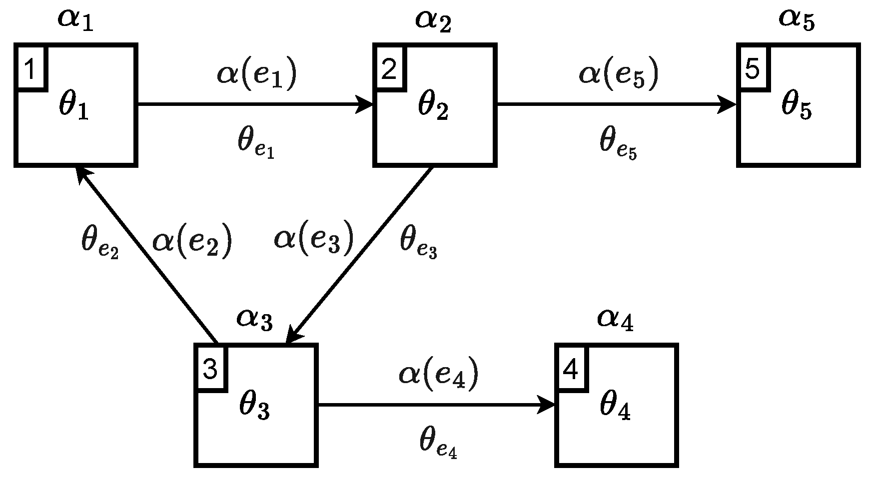
Given $S\subseteq G$, and $Q\in \mathcal{Q}$, we say that S matches Q ($S\vDash Q$), if the following formula holds:

$$Q\left(S\right)=\underset{n\in V_Q}{\bigwedge }{Q}_n^{\alpha \left(n\right)}\left(S\right)$$

where, for each node, $n\in V_Q$:

$$Q_n^{+}=Q_n,Q_n^{-}=\neg Q_n,$$

$$Q_n\left(S\right)=\exists v\in V\left(\underset{e\in \gamma \left(n\right)}{\bigwedge }{Q}_{e^{*}}^{\alpha \left(e\right)}(v,S)\right)$$

and, for each edge, $e\in E_Q$, $\ast \in \{o,i\}$:

$$Q_{e^{*}}^{+}=Q_{e^{*}},Q_{e^{*}}^{-}=\neg Q_{e^{*}},$$

$$Q_{e^o}(v,S)=\exists \rho \in {\mathcal{P}}_v^o\left(G\right)\left({\theta }_e(\rho ,S)\wedge {\theta }_{e^o}({\rho }^o,S)\wedge {\theta }_{e^i}({\rho }^i,S)\right),$$

$$Q_{e^i}(v,S)=\exists \rho \in {\mathcal{P}}_v^i\left(G\right)\left({\theta }_e(\rho ,S)\wedge {\theta }_{e^o}({\rho }^o,S)\wedge {\theta }_{e^i}({\rho }^i,S)\right).$$

A generic query example is shown in Figure 1.

Unlike other previous graph query systems, this system can efficiently satisfy the following requirements: (1) The ability to contain cycles; (2) the capability to evaluate subgraphs; (3) projecting edges in the query onto paths in the graph; (4) evaluating structural and/or semantic characteristics; and (5) the added benefit of specialization through atomic operations (as will be discussed in the next section).

3.3. Refinement Sets

To properly characterize the elements within a graph, it is crucial to utilize computationally effective methods when constructing queries based on basic operations. This section will introduce a query construction method optimized for use in relational learning tasks. To begin, let us first define the concept of relative refinements between queries.

Definition 7.

Given $Q_1,Q_2\in \mathcal{Q}$, we say:

1. 

$Q_1$ refines $Q_2$ in G ($Q_1{⪯}_G{Q}_2$) if: $\forall S\subseteq G(S\vDash Q_1\Rightarrow S\vDash Q_2)$.

2. 

They are equivalent in G ($Q_1{\equiv }_G{Q}_2$) if: $Q_1{⪯}_G{Q}_2$ and $Q_2{⪯}_G{Q}_1$.

Two queries are deemed equivalent when they are confirmed to be exactly the same by identical subgraphs. From this definition, it is straightforward the following result is straightforward (the proof of which may be omitted):

Theorem 1.

${⪯}_G$ is a partial order in $\mathcal{Q}$. That is, for every $Q_1,Q_2,Q_3\in \mathcal{Q}$:

1. 

$Q_1{⪯}_G{Q}_1$.

2. 

$Q_1{⪯}_G{Q}_2\wedge Q_2{⪯}_G{Q}_1\Rightarrow Q_1{\equiv }_G{Q}_2$.

3. 

$Q_1{⪯}_G{Q}_2\wedge Q_2{⪯}_G{Q}_3\Rightarrow Q_1{⪯}_G{Q}_3$.

Next, we examine the relationship between the topological structure of a query and its functionality as a predicate on subgraphs. Generally, extracting the logical properties of the predicate from the structural properties of the graph that represents it is difficult. However, we can obtain useful conditions to manipulate the structures and modify the query’s semantics in a controlled manner.

Definition 8.

Given $Q_1,Q_2\in \mathcal{Q}$, we say that $Q_1$ is a $Q^{-}$-conservative extension of $Q_2$ ($Q_2{\subseteq }^{-}{Q}_1$) if:

1. 

$Q_2\subseteq Q_1$.

2. 

$\forall n\in V_{Q_2}^{-}\forall e\in {\gamma }_{Q_1}\left(n\right)\exists e^{\prime }\in {\gamma }_{Q_2}\left(n\right)(Q_e\equiv Q_{e^{\prime }})$.

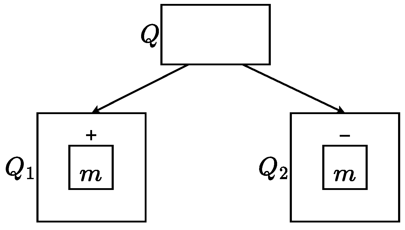
Figure 2 illustrates an example of a $Q^{-}$-conservative extension. The novel element in the right query mandates fresh constraints on the positive node, but it does not introduce any additional constraints to the negative one.

Since negative nodes introduce non-existence constraints to subgraph verification, $Q^{-}$-conservative extensions guarantee that no new constraints are added to them. Therefore,

Theorem 2.

If $Q_2{\subseteq }^{-}{Q}_1$ then $Q_1⪯Q_2$.

Proof. 

Since predicates associated with edges are solely based on the information within the edge itself (which takes into account the value of $\theta$ in its incident nodes, irrespective of their $\alpha$ value), we can assert that:

$$\forall e\in E_{Q_2}({Q_1}_e^{\alpha \left(e\right)}={Q_2}_e^{\alpha \left(e\right)})$$

Considering this fact, we examine the behavior of predicates associated with the nodes for both queries:

• If $n\in V_{Q_2}^{-}$, since $Q_2{\subseteq }^{-}{Q}_1$, then ${Q_1}_n^{-}={Q_2}_n^{-}$.
• If $n\in V_{Q_2}^{+}$, then ${Q_1}_n^{+}\to {Q_2}_n^{+}$, because (${\gamma }_1$, ${\gamma }_2$ are the incidence functions of $Q_1$ and $Q_2$, respectively):

  $$\begin{array}{cc}{Q_1}_n^{+}\hfill & =\exists v\in V\left(\underset{e\in {\gamma }_1\left(n\right)}{\bigwedge }{Q_1}_e^{\alpha \left(e\right)}\right)\hfill \\ \hfill & =\exists v\in V\left(\underset{e\in {\gamma }_1\left(n\right)\cap E_{Q_2}}{\bigwedge }{Q_1}_e^{\alpha \left(e\right)}\wedge \underset{e\in {\gamma }_1\left(n\right)\setminus E_{Q_2}}{\bigwedge }{Q_1}_e^{\alpha \left(e\right)}\right)\hfill \\ \hfill & =\exists v\in V\left(\underset{e\in {\gamma }_2\left(n\right)\cap E_{Q_2}}{\bigwedge }{Q_2}_e^{\alpha \left(e\right)}\wedge \underset{e\in {\gamma }_1\left(n\right)\setminus E_{Q_2}}{\bigwedge }{Q_1}_e^{\alpha \left(e\right)}\right)\hfill \\ \hfill & \to {Q_2}_n^{+}\hfill \end{array}$$

Hence,

$$\begin{array}{cc}{Q}_1\hfill & =\underset{n\in V_{Q_1}}{\bigwedge }{Q_1}_n^{\alpha \left(n\right)}=\underset{n\in V_{Q_2}}{\bigwedge }{Q_1}_n^{\alpha \left(n\right)}\wedge \underset{n\in V_{Q_1}\setminus V_{Q_2}}{\bigwedge }{Q_1}_n^{\alpha \left(n\right)}\hfill \\ \hfill & =\underset{n\in V_{Q_2}^{+}}{\bigwedge }{Q_1}_n^{\alpha \left(n\right)}\wedge \underset{n\in V_{Q_2}^{-}}{\bigwedge }{Q_1}_n^{\alpha \left(n\right)}\wedge \underset{n\in V_{Q_1}\setminus V_{Q_2}}{\bigwedge }{Q_1}_n^{\alpha \left(n\right)}\hfill \end{array}$$

$$\begin{array}{cc}\hfill & \to \underset{n\in V_{Q_2}^{+}}{\bigwedge }{Q_2}_n^{\alpha \left(n\right)}\wedge \underset{n\in V_{Q_2}^{-}}{\bigwedge }{Q_2}_n^{\alpha \left(n\right)}\wedge \underset{n\in V_{Q_1}\setminus V_{Q_2}}{\bigwedge }{Q_1}_n^{\alpha \left(n\right)}\hfill \\ \hfill & =\underset{n\in V_{Q_2}}{\bigwedge }{Q_2}_n^{\alpha \left(n\right)}\wedge \underset{n\in V_{Q_1}\setminus V_{Q_2}}{\bigwedge }{Q_1}_n^{\alpha \left(n\right)}\hfill \\ \hfill & \to Q_2\hfill \end{array}$$

 □

Previous results suggest that a query can be refined by adding nodes (of any sign) and edges to the existing positive nodes, but because of the (negated) interpretation of predicates associated with negative nodes, care must be taken to maintain their neighborhood to be sure that adding more edges does not weaken the imposed conditions (which, consequently, will not provide refined predicates).

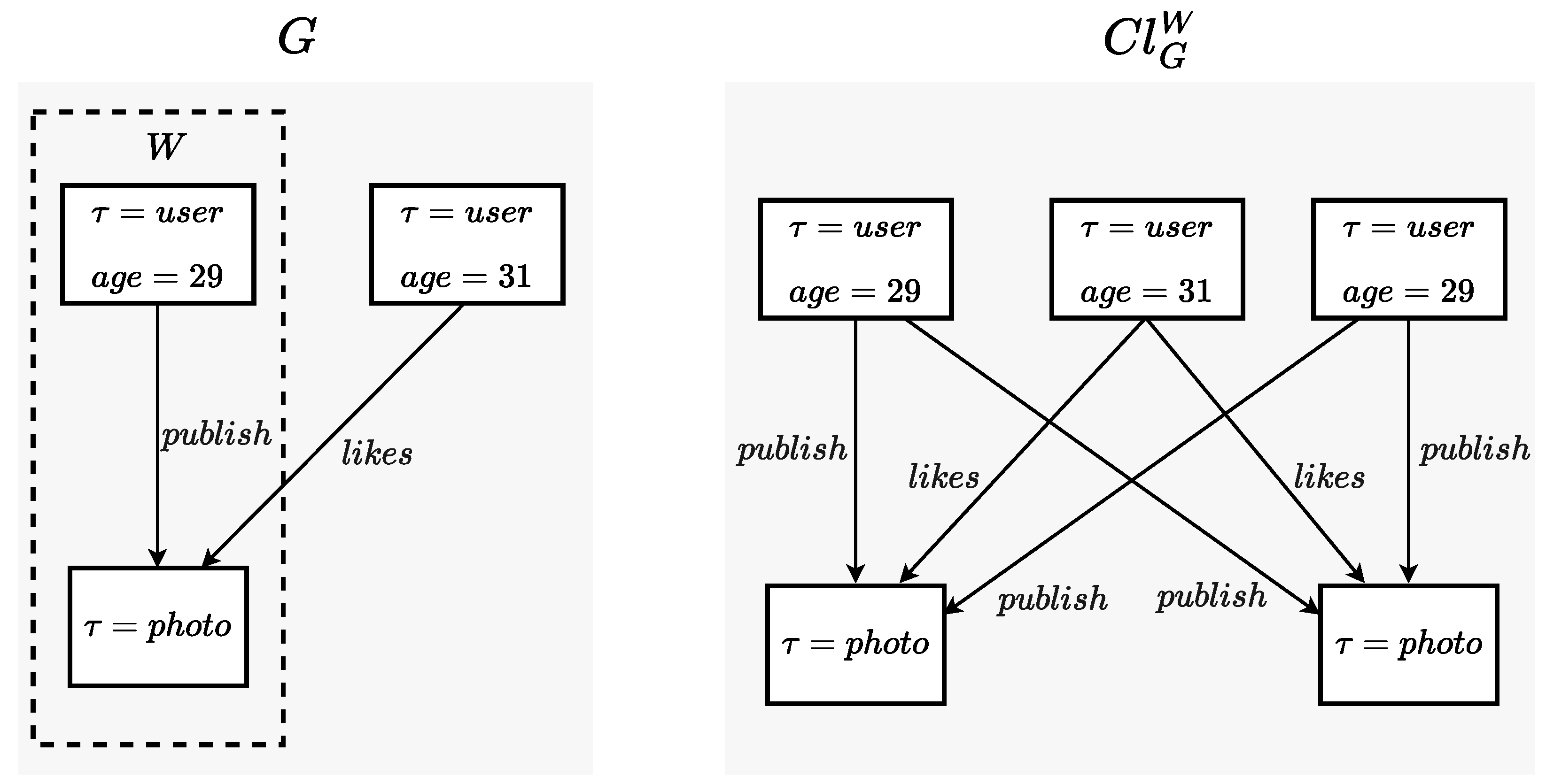
To achieve controlled methods of query generation, we will outline processes for refining queries through unit steps. We will accomplish this by defining the cloning operation, whereby existing nodes are duplicated, and all incident edges (including those between the nodes) on the original graph are also cloned:

Definition 9.

Given $G=(V,E,\mu )$, and $W\subseteq V$, we define the clone of G by duplication of W, $C{l}_G^W$, as:

$$C{l}_G^W=(V\cup W^{\prime },E\cup E^{\prime },\mu \cup {\left\{(n^{\prime },\mu \left(n\right))\right\}}_{n\in W}\cup {\left\{(e^{\prime },\mu \left(e\right))\right\}}_{e^{\prime }\in E^{\prime }})$$

where $W^{\prime }=\{n^{\prime }:n\in W\}$ are new cloned nodes from W, and $E^{\prime }$ is a set of new edges obtained from incident edges on nodes of W, where nodes of W are replaced by copies of $W^{\prime }$ (edges connecting original nodes with cloned nodes and edges connecting cloned nodes are cloned).

Figure 3 shows an example of a cloned graph by duplicating two nodes (in the original graph, left side, the node set to be duplicated is highlighted).

The next result indicates that duplicating positive nodes does not change the meaning of the queries.

Theorem 3.

If $W\subseteq V_Q^{+}$, then $C{l}_Q^W\equiv Q$.

Proof. 

Let us denote $Q_1=C{l}_Q^W$. Then:

$$\begin{array}{cc}{Q}_1\hfill & =\underset{n\in V_{Q_1}}{\bigwedge }{Q_1}_n^{\alpha \left(n\right)}=\underset{n\in V_Q}{\bigwedge }{Q_1}_n^{\alpha \left(n\right)}\wedge \underset{n\in W}{\bigwedge }{Q_1}_{n^{\prime }}^{\alpha \left(n^{\prime }\right)}\hfill \\ \hfill & =\underset{n\in V_Q\setminus {\gamma }_Q\left(W\right)}{\bigwedge }{Q_1}_n^{\alpha \left(n\right)}\wedge \underset{n\in {\gamma }_Q\left(W\right)}{\bigwedge }{Q_1}_n^{\alpha \left(n\right)}\wedge \underset{n\in W}{\bigwedge }{Q_1}_{n^{\prime }}^{\alpha \left(n^{\prime }\right)}\hfill \\ \hfill & =\underset{n\in V_Q\setminus {\gamma }_Q\left(W\right)}{\bigwedge }{Q}_n^{\alpha \left(n\right)}\wedge \underset{n\in {\gamma }_Q\left(W\right)}{\bigwedge }{Q}_n^{\alpha \left(n\right)}\wedge \underset{n\in W}{\bigwedge }{Q}_n^{\alpha \left(n\right)}\hfill \\ \hfill & =Q\hfill \end{array}$$

 □

When refining a query to find complementary sets of selected subgraphs, we define the concept of a refinement set as central:

Definition 10.

Given $Q\in \mathcal{Q}$, $R\subseteq \mathcal{Q}$ is a refinement set of Q in G if:

1. 

$\forall Q^{\prime }\in R\left(Q^{\prime }{⪯}_{G}Q\right).$

2. 

$\forall S\subseteq G(S\vDash Q\Rightarrow \exists !Q^{\prime }\in R(S\vDash Q^{\prime })).$

Let us now introduce refinement sets to enhance simpler queries for expressiveness. $Q\in \mathcal{Q}$ is prefixed, and ⊤ represents a tautology:

Theorem 4.

(Add new node) If $m\notin V_Q$, the set $Q+\left\{m\right\}$, formed by:

$$\begin{array}{cc}{Q}_1\hfill & =(V_Q\cup \left\{m\right\},E_Q,{\alpha }_Q\cup (m,+),{\theta }_Q\cup (m,\top )),\hfill \\ Q_2\hfill & =(V_Q\cup \left\{m\right\},E_Q,{\alpha }_Q\cup (m,-),{\theta }_Q\cup (m,\top ))\hfill \end{array}$$

is a refinement set of Q in G (Figure 4).

Proof. 

We must verify the two necessary conditions for refinement sets:

• Since $Q{\subseteq }^{-}{Q}_1$ and $Q{\subseteq }^{-}{Q}_2$, thus $Q_1⪯Q$ and $Q_2⪯Q$.
• Given $S\subseteq G$ such that $S\vDash Q$. Then:

  $$\begin{array}{cc}{Q}_1\hfill & =Q\wedge Q_m,\hfill \\ Q_2\hfill & =Q\wedge \neg Q_m\hfill \end{array}$$

  where $Q_m=\exists v\in V(\top )$.
  If $G\ne \varnothing$, then $S\vDash Q_1$ and $S⊭Q_2$.
  If $G=\varnothing$, then $S⊭Q_1$ and $S\vDash Q_2$.

 □

Since $G\ne \varnothing$ (usually), $Q_1\equiv Q$. However, although we obtain an equivalent query, this operation is beneficial for adding new nodes and restrictions in the future.

The second refinement allows for the establishment of edges between query nodes that already exist. To obtain a valid refinement set, the inclusion of edges is limited to positive nodes. Subsequently, the nodes marked with a positive/negative sign represent cloned nodes whose $\alpha$ property has been designated as positive/negative.

Theorem 5.

(Add a new edge between + nodes) If $n,m\in V_Q^{+}$, the set $Q+\left\{n\stackrel{e^{*}}{⟶}m\right\}$ ($\ast \in \{+,-\}$), formed by:

$$\begin{array}{cc}{Q}_1\hfill & =(V_{Q^{\prime }},E_{Q^{\prime }}\cup \left\{n^{+}\stackrel{e^{*}}{⟶}{m}^{+}\right\},{\theta }_{Q^{\prime }}\cup (e,\top )),\hfill \\ Q_2\hfill & =(V_{Q^{\prime }},E_{Q^{\prime }}\cup \left\{n^{+}\stackrel{e^{*}}{⟶}{m}^{-}\right\},{\theta }_{Q^{\prime }}\cup (e,\top )),\hfill \\ Q_3\hfill & =(V_{Q^{\prime }},E_{Q^{\prime }}\cup \left\{n^{-}\stackrel{e^{*}}{⟶}{m}^{+}\right\},{\theta }_{Q^{\prime }}\cup (e,\top )),\hfill \\ Q_4\hfill & =(V_{Q^{\prime }},E_{Q^{\prime }}\cup \left\{n^{-}\stackrel{e^{*}}{⟶}{m}^{-}\right\},{\theta }_{Q^{\prime }}\cup (e,\top ))\hfill \end{array}$$

(where $Q^{\prime }=C{l}_Q^{\{n,m\}}$) is a refinement set of Q in G (Figure 5).

Proof. 

• Since $Q^{\prime }$ is a clone of Q, then $Q\equiv Q^{\prime }$. In addition, $Q^{\prime }{\subseteq }^{-}{Q}_1,Q_2,Q_3,Q_4$, thus $Q_1,Q_2,Q_3,Q_4⪯Q^{\prime }\equiv Q$.
• Let us consider the predicates:

  $$\begin{array}{cc}{P}_n\hfill & =\exists v\in V\left(\underset{a\in \gamma \left(n\right)}{\bigwedge }{Q}_a^{\alpha \left(a\right)}\wedge Q_{e^o}^{\alpha \left(e\right)}\right),\hfill \\ P_m\hfill & =\exists v\in V\left(\underset{a\in \gamma \left(m\right)}{\bigwedge }{Q}_a^{\alpha \left(a\right)}\wedge Q_{e^i}^{\alpha \left(e\right)}\right).\hfill \end{array}$$
  If $S\vDash Q_n$ and $S\vDash Q_m$, then we have four mutually complementary options:
  • $S\vDash P_n\wedge S\vDash P_m\Rightarrow S\vDash Q_1$
  • $S\vDash P_n\wedge S⊭P_m\Rightarrow S\vDash Q_2$
  • $S⊭P_n\wedge S\vDash P_m\Rightarrow S\vDash Q_3$
  • $S⊭P_n\wedge S⊭P_m\Rightarrow S\vDash Q_4$

 □

Next, an additional predicate is added to an existing edge through the following operation, limited to positive edges connecting positive nodes.

Theorem 6.

(Add predicate to + edge between + nodes) If $n,m\in V_Q^{+}$, with $n\stackrel{e^{+}}{⟶}m$, and $\phi \in For{m}^2\left(L\right)$, the set $Q+\left\{n\stackrel{e\wedge \phi }{⟶}m\right\}$, formed by:

$$\begin{array}{cc}{Q}_1\hfill & =(V_{Q^{\prime }},E_{Q^{\prime }}\cup \{n^{+}\stackrel{e^{\prime }}{⟶}{m}^{+}\},{\theta }_{Q^{\prime }}\cup (e^{\prime },{\theta }_e\wedge \phi )),\hfill \\ Q_2\hfill & =(V_{Q^{\prime }},E_{Q^{\prime }}\cup \{n^{+}\stackrel{e^{\prime }}{⟶}{m}^{-}\},{\theta }_{Q^{\prime }}\cup (e^{\prime },{\theta }_e\wedge \phi )),\hfill \\ Q_3\hfill & =(V_{Q^{\prime }},E_{Q^{\prime }}\cup \{n^{-}\stackrel{e^{\prime }}{⟶}{m}^{+}\},{\theta }_{Q^{\prime }}\cup (e^{\prime },{\theta }_e\wedge \phi )),\hfill \\ Q_4\hfill & =(V_{Q^{\prime }},E_{Q^{\prime }}\cup \{n^{-}\stackrel{e^{\prime }}{⟶}{m}^{-}\},{\theta }_{Q^{\prime }}\cup (e^{\prime },{\theta }_e\wedge \phi ))\hfill \end{array}$$

(where $Q^{\prime }=C{l}_Q^{\{n,m\}}$) is a refinement set of Q in G (Figure 6).

Proof. 

The proof is similar to the previous ones. □

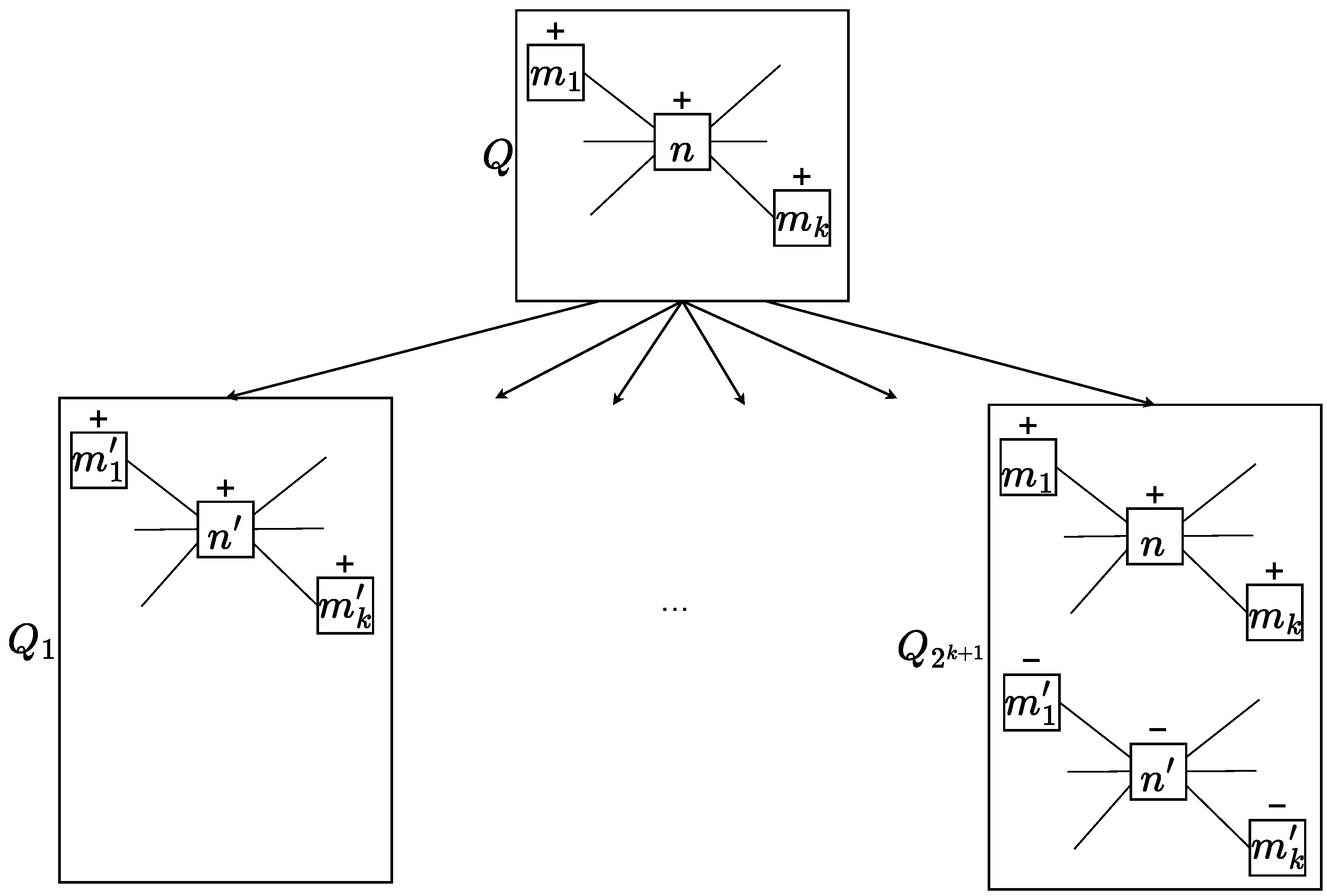
Finally, the last step involves adding predicates to existing nodes. This operation is only permitted when the affected nodes are positive, including the node where the predicate is added and those connected to it.

Theorem 7.

(Add predicate to + node with + neighborhood) If $\phi \in For{m}^2\left(L\right)$, and $n\in V_Q^{+}$ with ${\mathcal{N}}_Q\left(n\right)\subseteq V_Q^{+}$, then the set $Q+\{n\wedge \phi \}$ formed by:

$$\{Q_{\sigma }=(V_{Q^{\prime }},E_{Q^{\prime }},{\alpha }_{Q^{\prime }}\cup \sigma ,{\theta }_{Q^{\prime }}\cup (n^{\prime },{\theta }_n\wedge \phi )):\sigma \in {\{+,-\}}^{{\mathcal{N}}_Q(n)}\}$$

(where $Q^{\prime }=C{l}_Q^{{\mathcal{N}}_Q\left(n\right)}$, and ${\{+,-\}}^{{\mathcal{N}}_Q\left(n\right)}$ is the set of all possible assignments of signs to elements in ${\mathcal{N}}_Q\left(n\right)$) is a refinement set of Q in G (Figure 7).

Proof. 

The proof resembles earlier ones. It is important to consider that modifying node n not only alters the associated predicate but also those of its neighboring nodes. Additionally, the set of functions ${\{+,-\}}^{{\mathcal{N}}_Q\left(n\right)}$ encompasses all feasible sign assignments for the nodes within the neighborhood. □

Also note that simplified versions of the refinement sets are shown in Figure 4, Figure 5, Figure 6 and Figure 7. Section 3.4 explains how to obtain these simplifications.

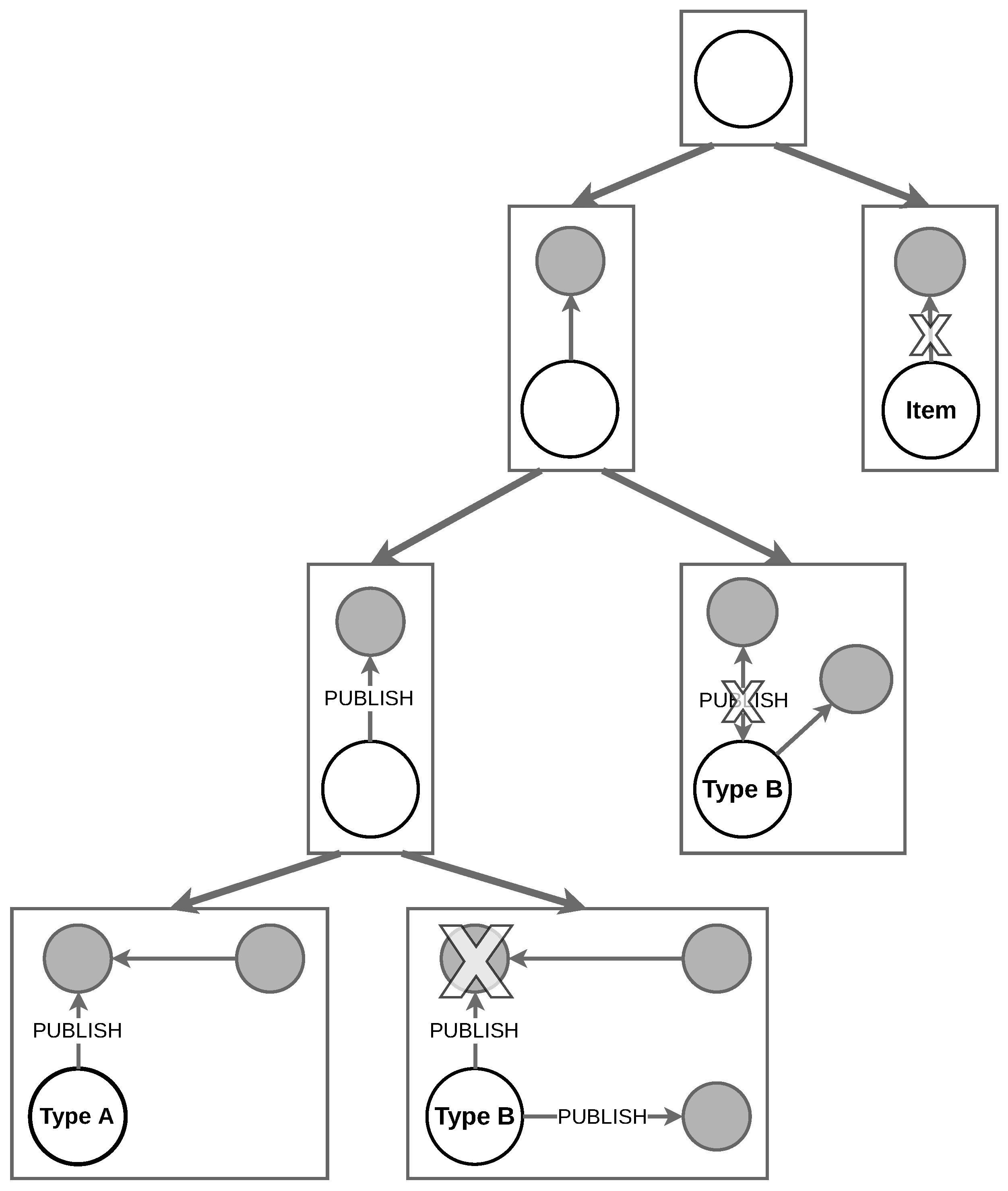
Obtaining a complementary query from the structure is a challenging task. Nonetheless, graph analyses often require sequences of queries to verify properties related to refinement and complementarity. To bridge this gap, this section introduces refinement operations. These operations facilitate the construction of an embedded partition tree, where nodes are labeled as illustrated in Figure 8:

• The root node is labeled with $Q_0$ (some initial query).
• If a node on the tree is labeled with Q, and $R=\{Q_1,\dots ,Q_n\}$ is a set that refines Q, then the child nodes will be labeled with the elements of R.

Refinement sets presented herein offer one approach, rather than the sole approach. For example, we could consider refinements that, instead of adding constraints to positive elements, lighten the conditions over negative elements, for example, by using disjunction of predicates instead of conjunction of them.

3.4. Simplified Refinement Sets

Let us simplify a query into an equivalent one by applying certain operations.

Definition 11.

We define $Q^{\prime }\subseteq Q$ as redundant in Q if $Q\equiv Q-Q^{\prime }$. Here, $Q-Q^{\prime }$ represents the subgraph of Q given by

$$(V_Q\setminus V_{Q^{\prime }},E_Q\setminus (E_{Q^{\prime }}\cup \{\gamma \left(n\right):n\in V_{Q^{\prime }}\}),{\mu }_Q)$$

One initial finding that enables the acquisition of simplified versions of a query by eliminating superfluous nodes is as follows (note that from the following two results, we only give an idea of the proof, which can be very laborious but straightforward from the above constructions):

Theorem 8.

Given a query Q, and $n,m\in V_Q$ verifying:

• $\alpha \left(n\right)=\alpha \left(m\right)$
• ${\theta }_n\equiv {\theta }_m$
• For each $e\in \gamma \left(n\right)$, exists $e^{\prime }\in \gamma \left(m\right)$, with $\alpha \left(e\right)=\alpha \left(e^{\prime }\right)$, ${\theta }_e\equiv {\theta }_{e^{\prime }}$ and $\gamma \left(e\right)\setminus \left\{n\right\}=\gamma \left(e^{\prime }\right)\setminus \left\{m\right\}$

Then, n is redundant in Q.

Proof. 

A query (Q) comprises nodes and their relationships. Each query node imposes constraints on the subgraph that is evaluated, including the presence or absence of nodes and the paths in which they participate. These restrictions should be considered during the evaluation. If there are two nodes, $n,m\in V_Q$, with $\alpha \left(n\right)=\alpha \left(m\right)$ and ${\theta }_n\equiv {\theta }_m$, and for each $e\in \gamma \left(n\right)$, there exists $e^{\prime }\in \gamma \left(m\right)$, with $\alpha \left(e\right)=\alpha \left(e^{\prime }\right)$, ${\theta }_e\equiv {\theta }_{e^{\prime }}$ and $\gamma \left(e\right)\setminus \left\{n\right\}=\gamma \left(e^{\prime }\right)\setminus \left\{m\right\}$, both nodes apply identical restrictions to the subgraph being evaluated. Therefore, deleting one of them will not change the assessment on the subgraph. □

In particular, m is a duplicate of n, but potentially with additional connected edges. A comparable outcome for the edges can be achieved:

Theorem 9.

Given a query Q, and two edges, $e,e^{\prime }\in E_Q$, such that $\alpha \left(e\right)=\alpha \left(e^{\prime }\right)$, $n\stackrel{e}{⟶}m$ and $n\stackrel{e^{\prime }}{⟶}m$ with $n,m\in V_Q^{+}$. If ${\theta }_e\to {\theta }_{e^{\prime }}$ then $e^{\prime }$ is redundant in Q.

Proof. 

Following the same reasoning as the previous theorem, if there are two edges, e and $e^{\prime }$, in $E_Q$, which connect the same two nodes in a query and $\alpha \left(e\right)=\alpha \left(e^{\prime }\right)$ and ${\theta }_e\to {\theta }_{e^{\prime }}$, the constraint imposed by e implies the constraint imposed by $e^{\prime }$. Therefore, eliminating $e^{\prime }$ would maintain the set of matching subgraphs. □

From these two findings, we can streamline the refinement sets that were established in Section 3.3 by removing redundant elements in succession after cloning.

3.5. Graph Query Examples

For illustrative purposes, this section presents a series of queries on a toy graph dataset. Figure 9 illustrates a segment of the Star Wars graph (http://console.neo4j.org/?id=StarWars, accessed on 1 September 2023).

To streamline query and graph representation, we will convert $\tau$, a property denoting node and edge types, into labels for edges or icons for nodes. Additionally, the node properties denoted by name will be written on them, and the undirected edges will be represented by bidirectional arrows. The property $\alpha$ will be represented directly on the query elements using $+/-$ symbols, and we will write the binary predicate $\theta$ directly on the elements (except for tautologies). When expressions such as $\tau \left(\rho \right)=X$ are in the predicate of an edge, X is written directly and interpreted as a regular expression to be verified by the sequence of $\tau$ properties of the links in the associated graph path.

Query 1 (Figure 10) can be interpreted as follows: Two characters are connected by a TEACHES relationship, where the master is over 500 years old and both are devoted to the Jedi. This query utilizes structural constraints through the presence of edges and predicates with properties such as $\tau$, name, and age. For example, in Figure 9, the subgraph comprising Yoda, Luke, and their TEACHES relationship satisfies this query.

Query 2 (Figure 11) outlines a cyclic query that utilizes the FRIENDS relationships. It can be verified on any subgraph containing three characters who are friends with each other (for example, the subgraph formed by Han Solo, Chewbacca, Princess Leia, and the FRIENDS relationships in Figure 9).

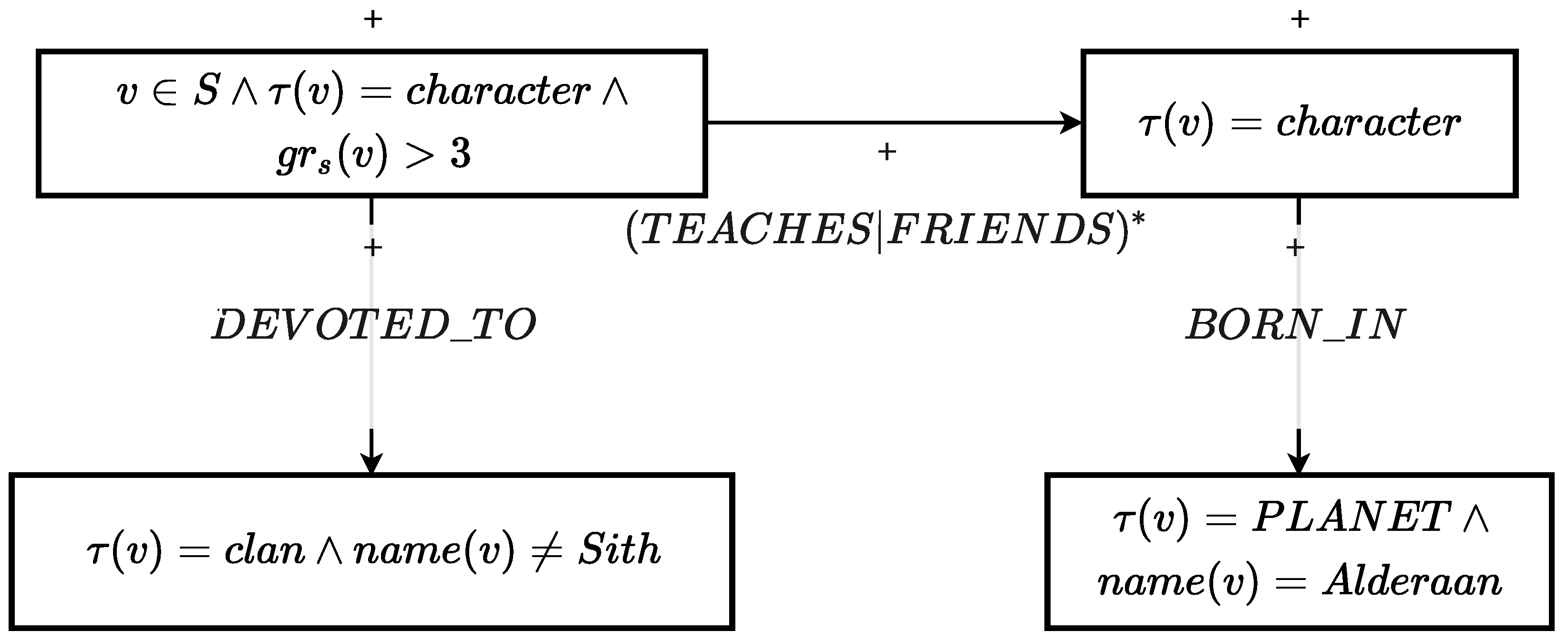
Query 3 (Figure 12) can be interpreted as follows: A character with more than three outgoing relationships, not belonging to the Sith clan, connected through a path consisting of any number of FRIENDS and TEACHES relationships with an individual from Alderaan. In this scenario, a regular expression is employed to denote a path consisting of an unspecified amount of FRIENDS and TEACHES relationships. Additionally, an auxiliary function, $g{r}_s\left(v\right)\in L$, is utilized to reference the outgoing degree of node v. This query will be validated by any subgraph that contains Luke or Obi-Wan Kenobi.

3.6. Computational Complexity

Query systems based on graph isomorphisms (most of the existing ones) face NP-complete complexity [34,35].

The preceding section presented our graph query framework that is reliant on logical predicates. In this section, we will demonstrate that the assessment of queries is polynomial, even in the case of cyclic queries. This is achievable by imposing two constraints. First, the length of paths that are illustrated by links in the query is restricted by the constant k, and second, the complexity of the predicates used in nodes and edges is polynomial.

To verify $S\vDash Q$, it is necessary to examine each predicate $Q_n\left(S\right)$ linked to all nodes $n\in V_Q$. Furthermore, each predicate $Q_n\left(S\right)$ linked to a node in Q requires assessing one $Q_e(v,S)$ predicate for every link $e\in {\gamma }_Q\left(n\right)$. Thus, initially, we focus on evaluating the computational complexity linked with the link predicates $Q_e(v,S)$. Subsequently, we will examine the complexity associated with the node predicates $Q_n\left(S\right)$. Ultimately, we will show that the query complexity is polynomial.

As previously defined, the computational complexity of evaluating predicates attributed to both nodes and edges within a query (Q) is polynomial, denoted by $\mathcal{O}\left(p\right)$. The predicates $Q_e(v,S)$ related to edges in a query verify the existence of a path $\rho$ in the graph G starting/ending in v that satisfies its own predicate ${\theta }_e(\rho ,S)$ and with the source and destination nodes that satisfy the predicates ${\theta }_{e^o}({\rho }^o,S)$ and ${\theta }_{e^i}({\rho }^i,S)$, respectively. Thus, the complexity involved in evaluating a particular path is $\mathcal{O}\left(3p\right)=\mathcal{O}\left(p\right)$.

The computational complexity to verify the existence of a path beginning or ending at a node v in V, satisfying the aforementioned criteria, is $\mathcal{O}(p\times |V{|}^k)$. Here, ${\left|V\right|}^k$ denotes the number of paths that start or end at v under the condition that they are no longer than k in length. As the number of links commencing or ending at a node $n\in V_Q$ is bound by $|E_Q|$, the computational complexity involved in the node predicate $Q_n\left(S\right)$ is $\mathcal{O}(p\times |V{|}^k\times \left|E_Q\right|)$.

Finally, if the query consists of $|V_Q|$ nodes, the complexity of checking the query $Q\left(S\right)$ is $\mathcal{O}(p\times |V{|}^k\times \left|E_Q\right|\times \left|V_Q\right|)$. It is evident that the constant k (path length bound) significantly impacts the execution of such queries, as it determines the exponent of the complexity.

The efficient operation of a graph query framework is crucial when dealing with large-scale datasets that are commonly found in real-world applications. Notably, when such a system is employed as the kernel of relational machine learning algorithms, as we will demonstrate in the following section, the ability to perform query operations in polynomial time, even for cyclic queries, is fundamental.

4. Relational Machine Learning

In this section, we will leverage the advantages of the framework presented to acquire relational classifiers on graph datasets. To elaborate, we will initiate from a labeled subgraph set within a graph dataset and then develop a pattern search technique founded on information gain to obtain typical patterns for each subgraph class.

4.1. Information-Gain Pattern Mining

To obtain characteristic patterns of subgraph classes using the previous graph query framework, a top-down decision tree induction will be conducted to explore the pattern space. Within the trees’ internal nodes, graph queries will serve as test tools. The best refinement sets will be identified during the tree construction process, resulting in queries that define classes within the graph dataset.

The training set, $\mathcal{L}$, consists of pairs $(S_i,y_i)$, where $S_i$ denotes a subgraph of G, and $y_i$ represents its associated class. Every node (n) in the resulting decision tree is linked to:

• A subset of the training set: ${\mathcal{L}}_n\subseteq \mathcal{L}$;
• A query $Q_n$, such that: $\forall S\in {\mathcal{L}}_n(S\vDash Q_n)$.

The tree learning procedure is standard: A tree is initialized comprising one node (the root) linked to the entire set of training, $\mathcal{L}$. The initial query, $Q_0$, corresponds to all its constituents ($\forall S\in \mathcal{L},S\vDash Q_0$). The subsequent stage involves determining which refinement set generates the maximum information gain while separating $\mathcal{L}$, and applying it to $Q_0$. For each query in the refinement set, a corresponding child node is created, and $\mathcal{L}$ samples are transmitted through it. A child with a matching associated query is guaranteed to exist since it is a refinement set of $Q_0$. The recursive process continues for each new node until a stop condition is met. At that point, the node becomes a leaf associated with a class. Note that the decision trees derived from this approach are not predominantly binary, unlike the prevalent trees in the literature.

4.2. Relational Tree Learning Examples

Here, we introduce some practical instances to demonstrate the process of performing relational learning by using the query framework and refinement sets. The refinement operations will be as mentioned in Section 3.3. A critical factor is that all subgraphs in a decision node belong to the same class, which we require as the stopping condition. Initially, we will focus on node classification problems before proceeding to classify more intricate structures.

Consider the small social network illustrated in Figure 13, portraying users and items in a graph. The objective is to classify the nodes based on the patterns extracted from the dataset.

Beginning with a training set composed of all nodes in the graph, Figure 14 displays the relational decision tree acquired through the process elucidated in Section 4.1. Negative nodes/edges are identified with a cross, while nodes with predicate $\theta (v,S):=v\in S$ are larger and white in hue. This tree accurately assigns types (User A, User B, or Item) to all nodes in the graph by exploiting relational information from the network. Furthermore, on the leaves of the tree, distinctive patterns are acquired for each node type, which can be used to directly assess nodes and clarify future classifications.

Similarly, by utilizing each character node in the Star Wars toy graph (Figure 9) and the corresponding species property as a training dataset, the relational decision tree shown in Figure 15 categorizes and explains each character’s species in the graph. The leaf patterns of the tree characterize each species: human characters are born friends of Luke, droids are unborn friends of Luke, Wookiees are those born in Kashyyyk, etc.

5. Conclusions and Future Work

This paper’s main contribution consists of a novel framework for graph queries that permits the polynomial cyclic assessment of queries and refinements based on atomic operations. The framework’s ability to apply refinements in relational learning processes was also demonstrated. In addition, the presented framework fulfills several essential requirements. The system utilizes consistent grammar for both queries and evaluated structures. It allows the assessment of subgraphs beyond individual nodes and supports cyclic queries within polynomial time (where the length of the query path is limited). The system offers a controlled and automated query construction via refinements, and the refinement sets constitute embedded partitions of the evaluated structure set, making them effective tools for top-down learning techniques.

Graph isomorphism-based query systems exhibit exponential complexity when presented with cyclic queries. Additionally, if a projection is necessary for pattern verification, evaluating the non-existence of specific elements becomes difficult or even impossible. However, the query graph framework offered here assesses the existence/non-existence of paths and nodes in a graph rather than demanding isomorphisms, thus enabling the evaluation of cyclic patterns in polynomial time.

After conducting an initial and fully functional proof-of-concept implementation, the graph query framework’s capabilities have been demonstrated through experimentation. This methodology has been explicitly applied in relational learning procedures, as demonstrated in Section 4.2, and the results of these experiments have shown that interesting patterns can be extracted from relational data. This is of great significance in both explainable learning and automatic feature extraction tasks. The results’ graphs were obtained via our proof-of-concept implementation on a graph database and by employing the matplotlib library [36].

Despite the presented query definition utilizing binary graph datasets (rather than hypergraphs), it can be implemented on hypergraph data as well. This is due to the fact that the concept of a path, which connects pairs of nodes, is independent of the edge arity involved. For the sake of simplicity, and due to the absence of true hypergraph databases, our queries are limited to the binary case. Nevertheless, they can be adapted to more universal cases once the usage of hypergraphs becomes more widespread.

Also, in Section 3.3, a basic and reliable set of refinement operations is provided. However, these operations should not be considered as the most suitable solution for all types of learning tasks. To achieve complex queries and to prevent plateaus in the pattern space, more complex refinement families can be established. For example, it is possible to combine the add edge and adding property to an edge operations into one step, thereby reducing the number of steps required. If executed properly, unifying the refinements based on the frequency of structural occurrences in a graph, for instance, can lead to faster versions of learning algorithms at the expense of covering a broader query space. This work provides theoretical tools to support the accuracy of new refinement families. Future research will focus on developing automated methods to generate refinement sets based on a given learning task and the specific characteristics of the graph dataset. Extracting statistics from the graph data for the automatic generation of such sets can result in significant optimizations.

It is concluded that establishing effective techniques for matching graph patterns and learning symbolic relationships is feasible, resulting in a systematic exploration of the pattern space, a high degree of expressiveness in queries, and computational costs of implementations kept within reasonable order.

Patterns associated with the leaves in obtained decision trees can be used to characterize subgraph categories. Moreover, the path from the root node to the corresponding leaf of the decision tree for a particular input can be used to justify decisions; this is a beneficial feature in various sensitive applications, such as decision trees. In addition, patterns obtained from the graph learning procedure presented can serve as features in other machine learning methods. Once the patterns are acquired, they can serve as Boolean features for subgraph modeling, enabling non-relational machine learning methods to learn from them.

Learning of relational decision trees can be utilized by ensemble methods (such as random forest), and although the explanatory power is diluted when multiple trees are combined, their predictive power can be greatly enhanced. Therefore, it is essential to investigate the probabilistic amalgamation of queries to generate patterns that can be interpreted as probabilistic decision tools.

Furthermore, while a relational decision tree learning technique has been employed, additional machine learning algorithms can be evaluated alongside this query framework to investigate more opportunities for relational learning.