


Abstract
Prior research has consistently shown that students’ SAT scores are influenced by factors beyond academic ability, including socioeconomic background and ethnicity. Using aggregated school-level data from Massachusetts and New York City (NYC), this study assesses the quantitative relationships between average SAT scores and school-level demographics, academic preparation, and funding to inform education policy and equity efforts. Three analytical methods, multiple linear regression, relaxed Least Absolute Shrinkage and Selection Operator (LASSO), and decision trees, were applied sequentially to capture the linear and nonlinear associations. Across all three methods, socioeconomic disadvantage exhibited the strongest and most robust correlation of lower SAT scores, with racial composition and academic preparation identified as secondary factors. Schools with high percentages of Black, Hispanic, and low-income students tend to have lower average scores than schools with high percentages of White, Asian, and well-off students. Moreover, schools with higher college attendance rates and greater funding tend to exhibit higher average SAT scores. These findings represent school-level correlations rather than causal effects and indicate that SAT score disparities are closely intertwined with broader structural inequities already embedded within the K–12 education system. Accordingly, while targeted SAT preparation initiatives may offer modest benefits, meaningful reductions in observed disparities likely require broader policy interventions to expand equitable access to educational opportunities.
1. Introduction
The Scholastic Aptitude Test (SAT) was originally adapted from the Army intelligence quotient (IQ) Test. The first exam, administered in 1926, was used to test applicants to West Point and not for college admission. Grounded in the concept of aptitude, the SAT was designed to predict students’ academic performance by assessing their readiness for college-level work rather than mastery of specific curricular content. Its original purpose was to measure intellectual ability independently of school quality or family background.
The SAT entered higher education admissions largely through the influence of James Bryant Conant, who served as president of Harvard University from the 1930s to the 1950s. Conant adopted the SAT, then called the “Harvard Scholarship Test”, and required it for all applicants by 1941. At a time when college admissions heavily favored students from affluent backgrounds, Conant viewed the SAT as a tool to democratize access to elite education. By the late 1930s, the SAT had become a central component of admissions across Ivy League institutions and, by the 1990s, was required by most U.S. colleges and universities.
Criticism of standardized testing intensified in the early 2000s, giving rise to the test-optional movement, as critics argued that the tests were unfair because score gaps reflected racial and socioeconomic disparities. In 2001, the president of the University of California recommended that campuses discontinue using the SAT. Empirical evidence from Bates College played a pivotal role in renewing interest in test-optional policies. Bates adopted a test-optional policy in 1984 but continued to require scores from enrolled students to support long-term institutional research. Analyses of 20 years of data revealed negligible differences in college GPA between students who submitted SAT scores and those who did not, despite substantial differences in test scores (Hiss & Franks, 2014). These findings, alongside reports from organizations such as the National Association for College Admission Counseling (NACAC, 2008), prompted many liberal arts colleges to reconsider the role of standardized testing in admissions.
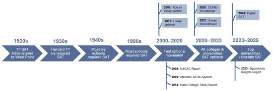
In response to growing criticism, the College Board redesigned the SAT multiple times, first by making the essay section optional in 2005 and eventually eliminating it in 2021. In 2024, the SAT transitioned to a digital format and was shortened. Although the test-optional movement gained momentum prior to 2020, the COVID-19 outbreak accelerated its adoption by forcing most institutions to suspend testing requirements. During this period, almost all universities adopted a test-optional policy due to the difficulty of administering tests safely.
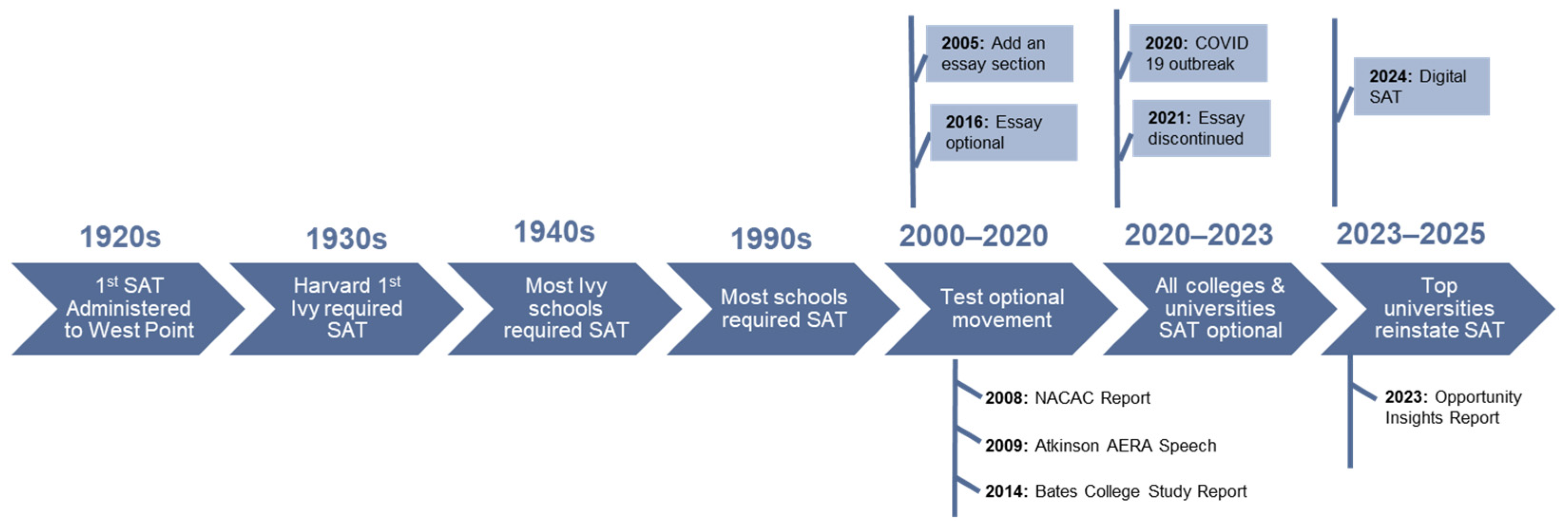
Following the easing of pandemic-related disruptions in 2023, several highly selective universities, including Harvard University and the Massachusetts Institute of Technology (MIT), however, reinstated SAT requirements for undergraduate admissions. In 2024, research from Opportunity Insights, a team of Harvard-based researchers and policy analysts, suggested that SAT scores are more predictive of post-college success than high school grades (Chetty et al., 2023). The major policy reports supporting this movement, along with changes made to SAT testing in response, are shown in Figure 1.
Figure 1.
Significant landmarks in the role of SAT in college and university admissions. Cited report references: 2008 NACAC report (NACAC, 2008), 2009 Atkinsons American Educational Research Association (AERA) Speech (Atkinson, 2009), 2014 Bates College Study Report (Hiss & Franks, 2014), 2025 Opportunity Insights Report (Chetty et al., 2023).
This history raises a fundamental question: are socioeconomic disparities a primary driver of SAT performance, or does the SAT merely reflect underlying inequalities in the education system? Most prior research addressing this question relies on individual-level student data, which is informative, but often overlooks broader school-level contexts. To address this gap, the present study analyzes aggregated school-level data to examine associations between average SAT scores and both compositional factors (e.g., racial/ethnic composition and economic disadvantage) and contextual characteristics (e.g., college attendance rates and school funding). A complementary set of analytical methods, including multiple linear regression, relaxed least absolute shrinkage and selection operator (LASSO), and decision tree models, was applied to identify robust patterns of association across multiple modeling frameworks.
Although the cross-sectional design precludes causal inference, this analysis provides important descriptive insights into how school context, socioeconomic and demographic composition are concurrent with SAT performance. These findings aim to help educators and policymakers understand structural patterns underlying observed score disparities and support broader efforts to promote educational equity and opportunity (Liu et al., 2024).
2. Related Work
The Coleman Report, titled “Equality of Educational Opportunity,” is a landmark study that analyzes the factors contributing to educational achievement (Coleman, 1966/2007). The report found that family background (especially parental education and income) was a stronger predictor of student performance than school facilities or resources. Since then, a substantial interdisciplinary literature has examined the relationship between student’s socioeconomic status (SES) and academic achievement. Research specifically addressing the relationship between family background and SAT performance expanded rapidly in the early 2000s, concurrent with the emergence of the test-optional movement. A list of previous studies on the relationship between family background and SAT performance is shown in Appendix A and their key findings are summarized below.
Studies conducted by the College Board have consistently documented a positive association between socioeconomic status (SES) and SAT scores. The results from Camara and Schmidt indicated that parental income and education are strongly related to performance on various measures, with parental education showing a stronger relationship (Camara & Schmidt, 1999). However, these authors noted that SES is not an isolated determinant but is closely linked to other factors and outcomes related to academic performance, including high school GPA and class rank.
Subsequent work by Sackett and colleagues reinforced the central role of socioeconomic background while highlighting the complexity of its relationship with standardized test outcomes (Sackett et al., 2009a, 2009b). Their analyses demonstrated that students from higher-income backgrounds tend to achieve higher SAT scores and that SAT scores predict subsequent college performance independently of SES (Sackett et al., 2012). These findings suggest that observed SES gradients in SAT performance likely reflect cumulative exposure to differential educational opportunities rather than short-term test preparation alone. This cumulative process may operate through sustained differences in school quality, curriculum rigor, peer environments, and other social factors (Sackett et al., 2012).
Research by Zwick further complicates the interpretation of SES effects by showing that SAT scores exhibit weaker associations with SES than other academic indicators such as high school grades and class rank (Zwick & Green, 2007; Zwick & Himelfarb, 2011). This pattern suggests that standardized test performance may reflect a narrower set of competencies than broader academic achievement, while still remaining sensitive to long-run differences in educational access and preparation.
An extensive literature has examined racial and ethnic disparities in SAT performance, many reporting that race retains an “independent” statistical association even after controlling for family income and parental education. An analysis by Dixon-Roman from a large dataset (781,437 Black and White college-bound high school students who took the SAT in 2003) suggested that students from higher-income families tend to earn higher SAT scores than their lower-income peers, with income-related score disparities being substantially larger among Black students than among White students (Dixon-Román et al., 2013). The findings of the Black–White SAT performance gap were consistent with studies published in The Journal of Blacks in Higher Education, which similarly documented the gap. This research demonstrated that measures of family economic background account for part of this disparity, suggesting that differences in family income alone do not fully account for racial and ethnic disparities in overall SAT scores (JBHE Foundation, 1998).
Large-scale analyses of California high school graduates applying to the University of California system further reinforce the roles of family background and ethnic background. Studies of over 1.6 million California high school graduates who applied to the UC system between 1994 and 2016 confirmed that SAT/ACT scores are most strongly influenced by family background, including low-income status, first-generation college attendance, and minority status (Geiser, 2015, 2017). Geiser’s analysis further demonstrated that race/ethnicity exerts an independent statistical effect on SAT/ACT scores, even after controlling family income and parental education. Conceptually, this “independent” effect is interpreted as a marker of historically produced school arrangements that shape educational opportunity, rather than as an inherent causal attribute.
A smaller but important body of research has incorporated school-level factors into analyses of SAT performance. One study by Kobrin used hierarchical linear modeling (HLM) to investigate student- and school-level predictors of score discrepancies, identifying school-level factors such as economic advantage and school size as significant predictors of a school’s average discrepancy score (Kobrin et al., 2003). Everson and Millsap examined both individual- and school-level contributions to SAT score gaps using multilevel latent variable modeling techniques. Their results indicated that, after accounting for school-level effects, the SAT performance gaps between different socioeconomic classes were reduced by an average of 50 points (Everson & Millsap, 2004). Another 2004 study suggested that differences in school quality may be a significant factor in the explanation (Fryer & Levitt, 2004). These findings suggest substantial disparities in the distribution of educational resources across schools, which in turn contribute to differences in SAT scores.
Despite these advances, we found that most existing studies have focused on individuals’ family backgrounds without accounting for the school environment in their analyses. The school-level factors, such as students’ accessibility to quality education, higher education culture, and school funding, and their impact on SAT scores, are rarely discussed. Furthermore, multicollinearity and interaction effects among socioeconomic and demographic, and school-level factors were, for the most part, not thoroughly examined.
Thus, there remains a need for closer investigation of the association of both compositional and contextual factors with SAT performance using a modeling framework capable of capturing complex interactions among factors. In this study, we aimed to address these gaps by developing a robust analytical approach to identify and quantify relationships between these factors and school SAT performance.
3. Method
The study utilized two SAT score datasets on Kaggle.com: Massachusetts (MA) Public Schools Data (Dalziel, 2017) and Average SAT Scores for New York City (NYC) Public Schools (Larion, 2016). The two datasets, licensed under CC0 (public domain), were chosen for their high usability scores (8.5 for MA data and 8.2 for NYC data) and clear documentation, labeling, and manageable size. The Massachusetts dataset includes student body (demographic distributions such as percentage of gender, ethnicity, economic situation), funding levels (class size, Per Pupil Expenditure), college attendance, and testing (SAT, MCAS, APs), and was compiled from the data in the Massachusetts Department of Education reports in 2017. The NYC dataset includes student races, neighborhoods, and average SAT scores for the 2014–2015 school year and was compiled and published by the New York City Department of Education.
In this study, we use R (R Core Team, 2024), version 4.4.1, for data processing, visualization, and model-based analysis of the actual and predicted data.
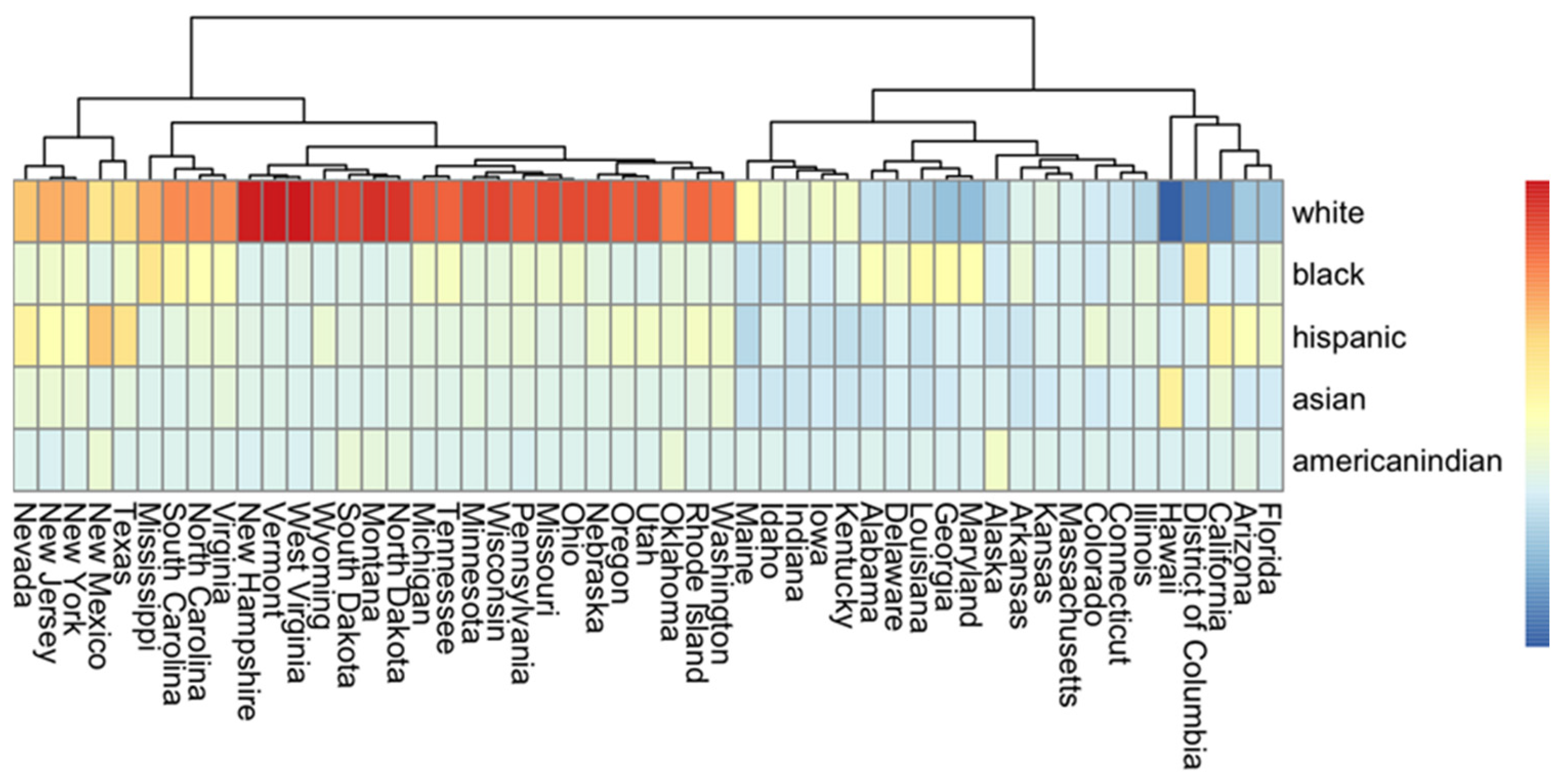
An Ontology heatmap comparing population distribution by race across all 50 states (KFF, 2017) was produced, which justifies our comparison between MA and NYC, as illustrated in Figure 2.
Figure 2.
The population distribution by race across all 50 states. The “pheatmap” function in R creates heat maps by mapping numerical matrix values to colors. The colors represent a relative difference from the state we chose as the center, Massachusetts. Percentages below Massachusetts were dark blue, middle values were white/light, and percentages above Massachusetts were dark red.
Based on the heatmap, states with population distributions similar to MA’s include Illinois, Connecticut, Colorado, Kansas, Arkansas, Alaska, Kentucky, Iowa, Indiana, and Idaho, suggesting we could generalize our MA predictions to these states. To further expand our analysis, we sought to explore a state with a different demographic profile from MA. As seen on the ontology map, New York had a drastically different population. To make data easier to find, we focused solely on NYC.
Data processing steps below were used to construct the analytical dataset for MA:
- Removed data from elementary and middle schools due to a lack of SAT scores.
- Removed irrelevant outcome variables (i.e., AP scores) as the analysis focused solely on SAT scores
- Renamed variables for operational simplicity
- Converted old SAT score (out of 2400) to new SAT score (out of 1600)
- Mutated the percentages to numbers for ease of computing; for example, 35% was represented as 35 rather than 0.35 in the analysis.
For the NYC dataset, we selected only race variables for analysis, removing other variables such as the percentage of students who took the test and school size. However, we kept these variables for data visualization. The NYC dataset did not contain the same variables as the Massachusetts dataset. After data preprocessing, 60 public high schools in NYC were excluded due to missing SAT score reports. The final analytic sample therefore comprised 295 of 295 public high schools in Massachusetts (100%) and 375 of 435 public high schools in New York City (86%).
3.1. Data Visualization
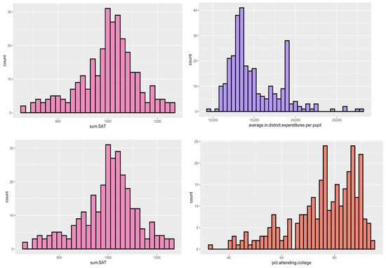
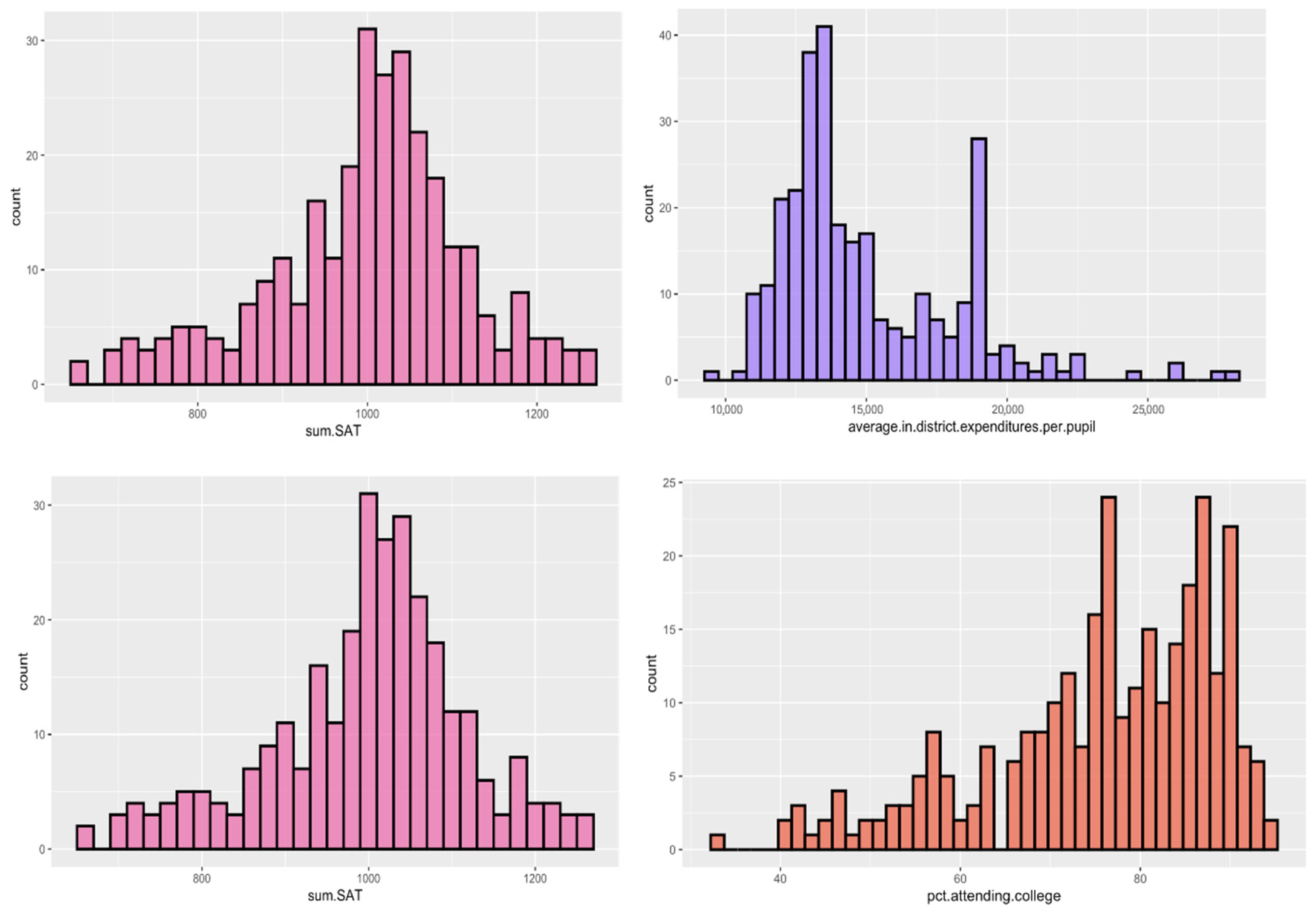
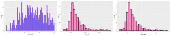
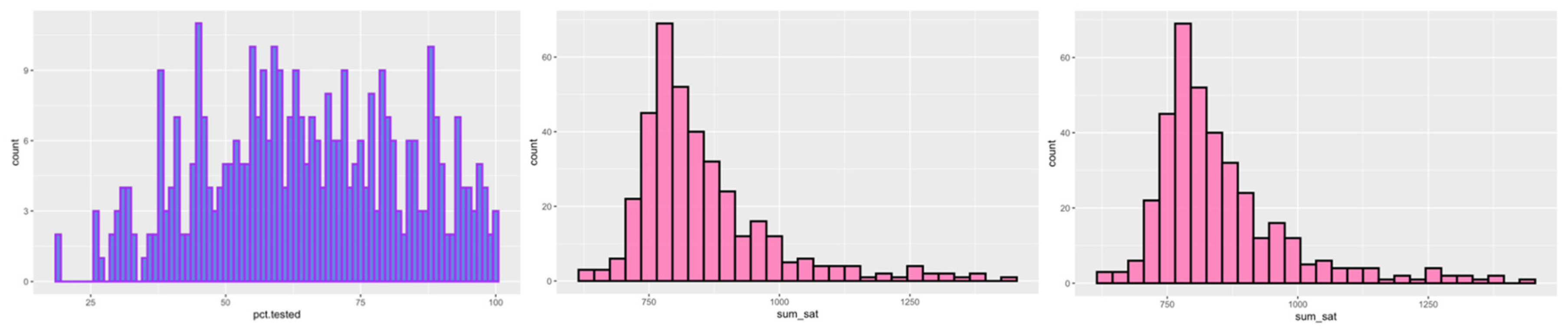
Data visualization tools, such as histograms, box plots, and heatmap analysis, were used to identify central tendencies and outliers in both datasets. First, we produced histograms of SAT scores in MA and NYC, as illustrated in Figure 3 and Figure 4. The mean SAT score for MA was around 1000, and the curve was bell-shaped, indicating a normal distribution. The mean SAT score in NYC was around 750; the curve was slightly right-skewed.
Figure 3.
Distribution of SAT scores and variables in the MA dataset.
Figure 4.
Distribution of SAT scores and variables in the NYC dataset.
For the MA dataset, additional school features, including average in-district expenditures per pupil, the percentage of economically disadvantaged students, and the percentage of people attending college, were also visualized in a histogram (Figure 3). The histogram showing expenditure per pupil at each school was skewed to the right with a mean expenditure around $13,000 and a noticeable outlier just before $20,000; The percentage of students economically disadvantaged was skewed right, meaning most schools had low mean percentage of eco-nomically disadvantaged students, around 10%; the percentage of people attending college was skewed to the right, indicating most schools had a high rate of students attending college, a mean of around 90%.
For the NYC dataset, histograms were also produced for the student enrollment and the percentage of students at the school who took the SAT (Figure 4). Student enrollment was right-skewed, with a mean of about 500 per school. The percentage tested per school followed a relatively normal distribution, with a mean of about 60%. Compared directly, the mean SAT score for MA is noticeably higher (1000 vs. 700). While the other data visualizations cannot be directly compared, they provide good context for the state/region.
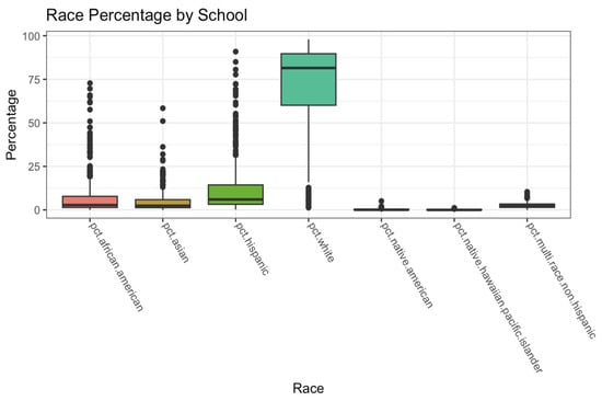
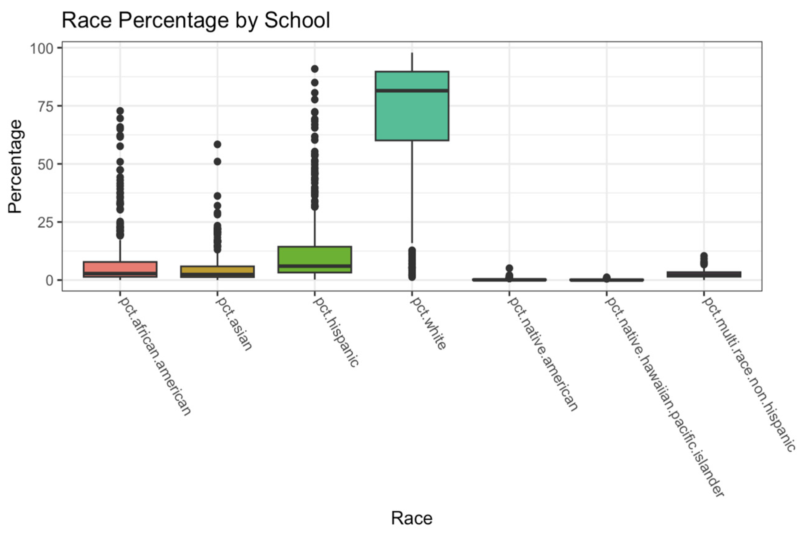
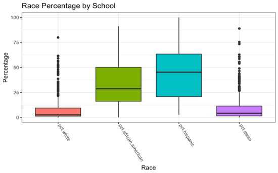
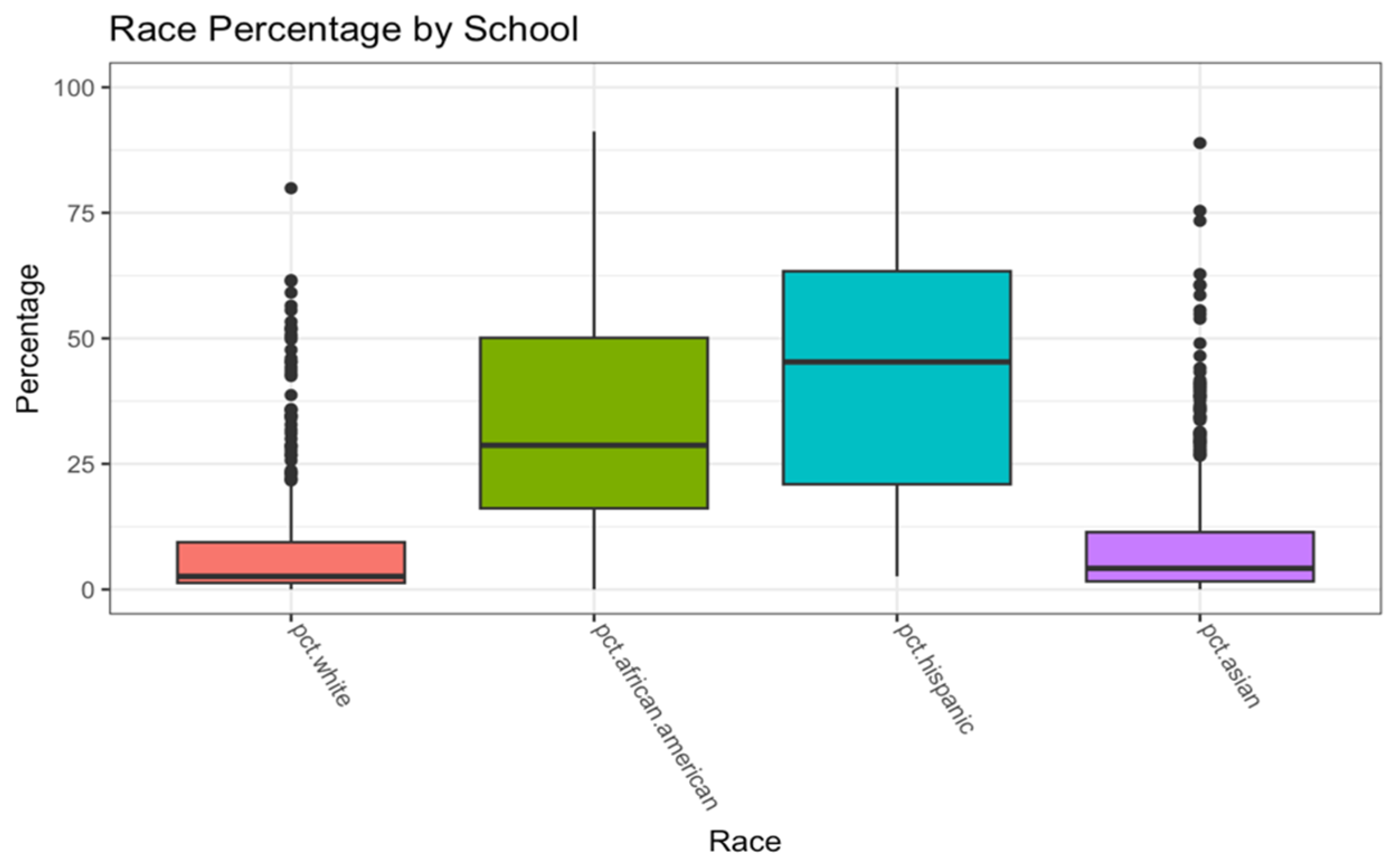
Furthermore, boxplots were generated to compare race percentages across schools in MA and NYC. As shown in Figure 5, MA schools generally have higher percentages of Caucasians than African Americans, Asians, and Hispanics (Figure 5). Conversely, in New York City, the percentages of Hispanics and African Americans are significantly higher than those of Caucasians and Asians (Figure 6).
Figure 5.
Race distribution in the Massachusetts dataset.
Figure 6.
Race distribution in the NYC dataset.
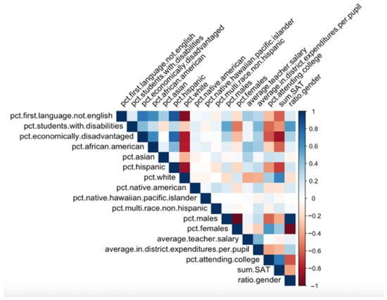
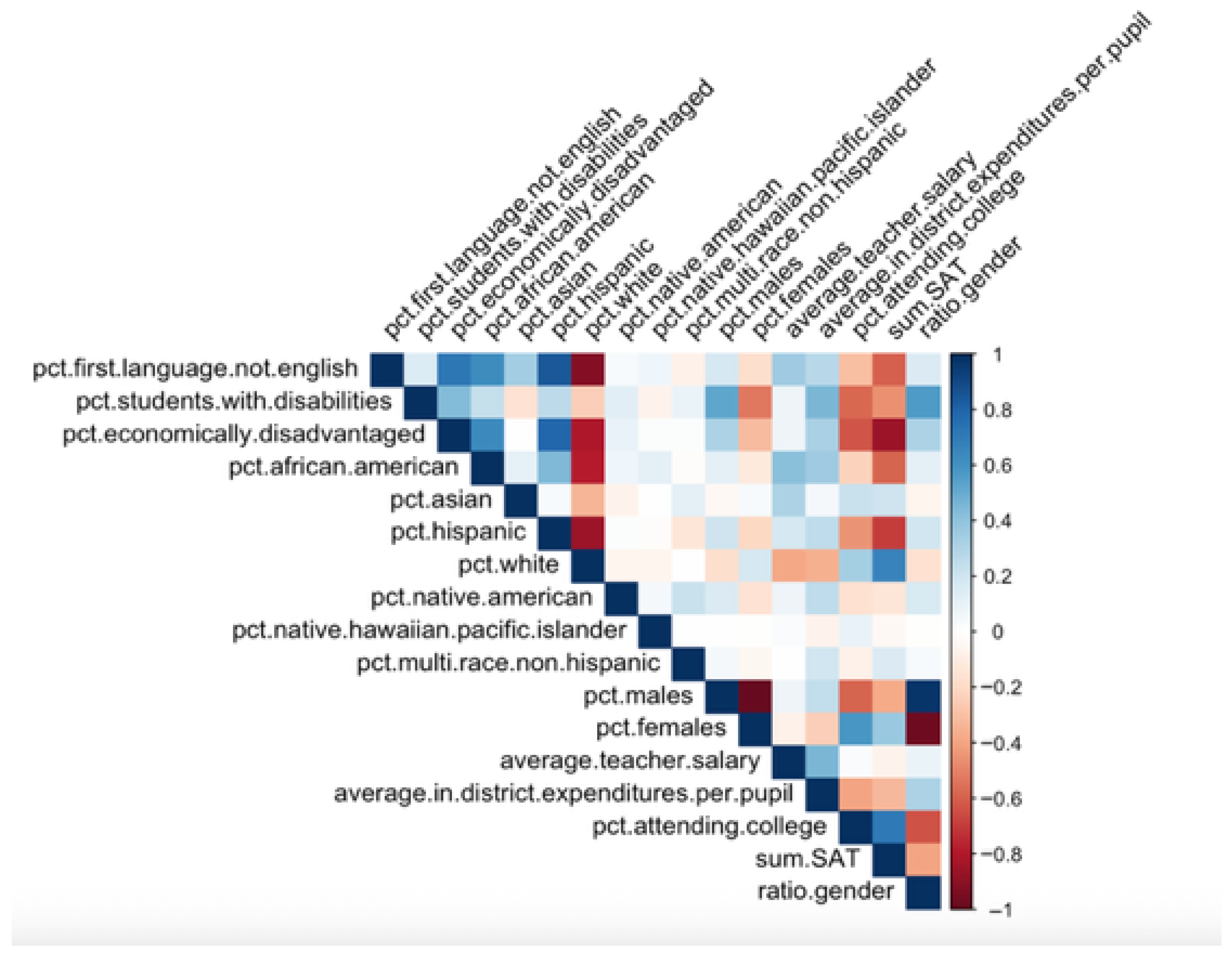
As shown in the MA correlogram (Figure 7), the percentage of economically disadvantaged individuals had a large positive correlation with the percentages of African Americans and Hispanics. This correlogram was not generated for the NYC dataset because it contained only race data.
Figure 7.
Multicollinearity between variables in the Massachusetts dataset.
3.2. Model-Based Analysis
Recognizing the collinearity between demographic factors and other factors on the school level, three analytical methods-multiple linear regression (MLR), relaxed Least Absolute Shrinkage and Selection Operator (LASSO), and decision trees, were applied sequentially to capture the linear and nonlinear associations. By combining these three methods, we leverage their complementary strengths: MLR provides a statistically interpretable baseline; relaxed LASSO performs robust variable selection while mitigating multicollinearity; and decision trees explore nonlinear relationships and higher-order interactions to capture the complexity of school environments with minimal sensitivity to collinearity. Together, these approaches enable a comprehensive, multi-perspective analysis of school-level factors associated with SAT performance.
3.2.1. Multiple Linear Regression (MLR)
MLR is especially useful for estimating the relationship between a single dependent variable (e.g., average SAT score) and multiple independent variables (e.g., race percentages). The coefficients it produces quantify how much the dependent variable is expected to change when the independent variable increases by 1 unit, while holding all other variables constant. We used this analysis first because it provides an interpretable baseline model that indicates the direction and magnitude of correlation. It also enables us to test for statistical significance and identify which predictors are meaningfully related to SAT scores. We used backward selection to retain only statistically significant predictors at the 0.001 level.
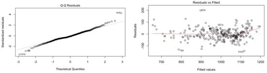
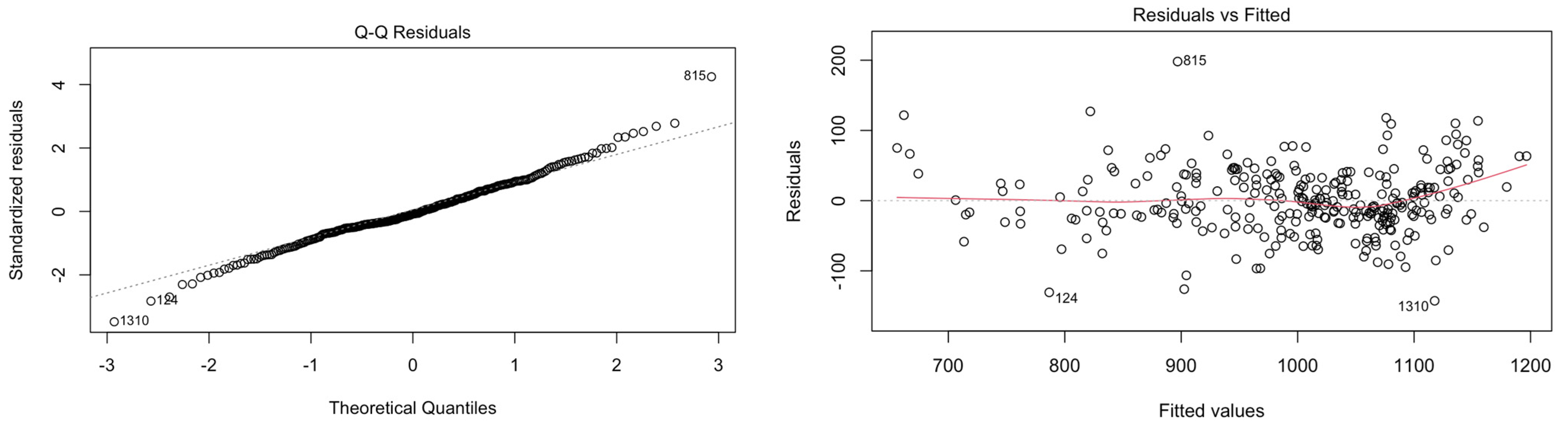
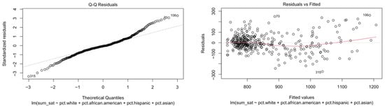
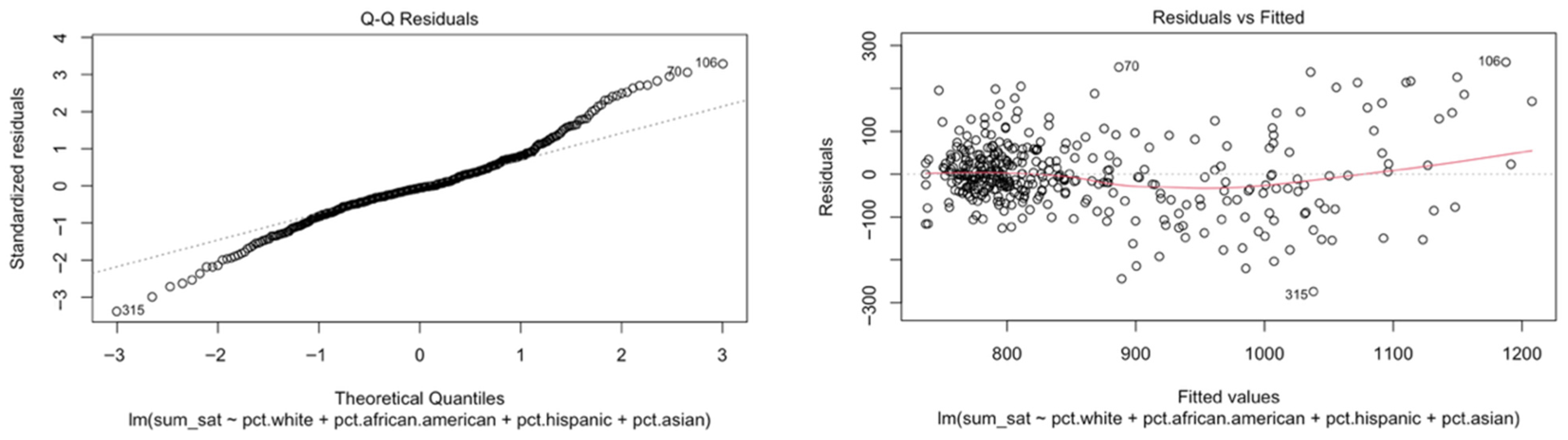
To validate our MLR assumptions, we used the plot function to create a Residual vs. Fitted plot and a normal QQ plot to assess homoscedasticity and linearity (Kim, 2015). For both MA and NYC, the Residual vs. Fitted plot showed an equal distribution of points above and below the line, indicating homoscedasticity. Our Normality QQplot demonstrated a linear relationship, indicating linearity (Figure 8 and Figure 9).
Figure 8.
Goodness of fit plots for the MLR model in the MA dataset.
Figure 9.
Goodness of fit plots for the MLR model in the NYC dataset.
Additionally, for each coefficient in the multiple linear regression model, we calculated a 95% confidence interval to quantify the uncertainty of the estimated effect. This allowed us to assess the magnitude and reliability of each predictor’s impact on SAT scores. Since none of the intervals include zero, this indicates the relationship between all the predictors and the SAT score is statistically significant.
The MLR modeling output and evaluation metrics, such as R2, mean squared error (MSE), root mean squared error (RMSE), variation inflation factor (VIF), and influence diagnostics plots, were reported in Appendix B.
3.2.2. Relaxed LASSO
Since regression models are sensitive to multicollinearity, it is common for demographic variables (e.g., race and economic disadvantages) to overlap. To address this, we used the Relaxed LASSO analytical method. Instead of keeping all correlated variables, it picks one variable from a correlated group, reducing overfitting. The relaxed LASSO also moves less relevant predictors towards zero and refits the model with less shrinkage on the selected variables (Tibshirani, 1996). While MLR outputs effect sizes, relaxed LASSO produces a more parsimonious model.
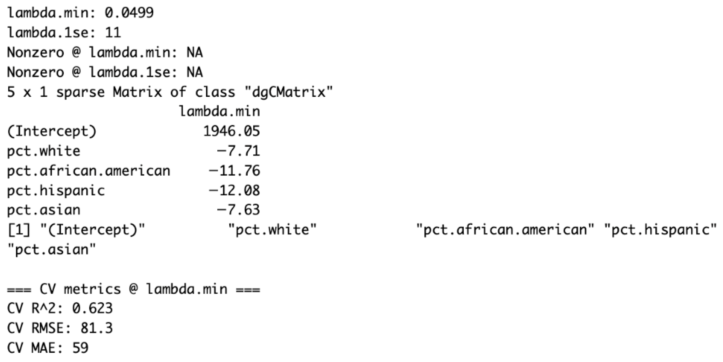
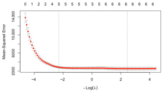
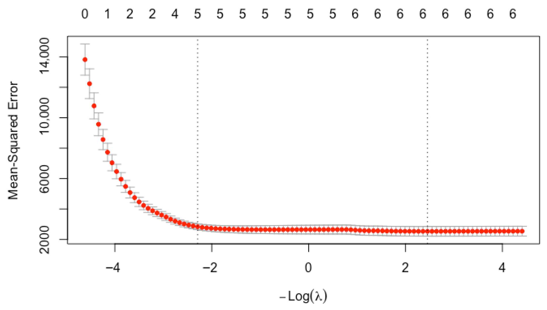
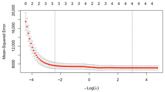
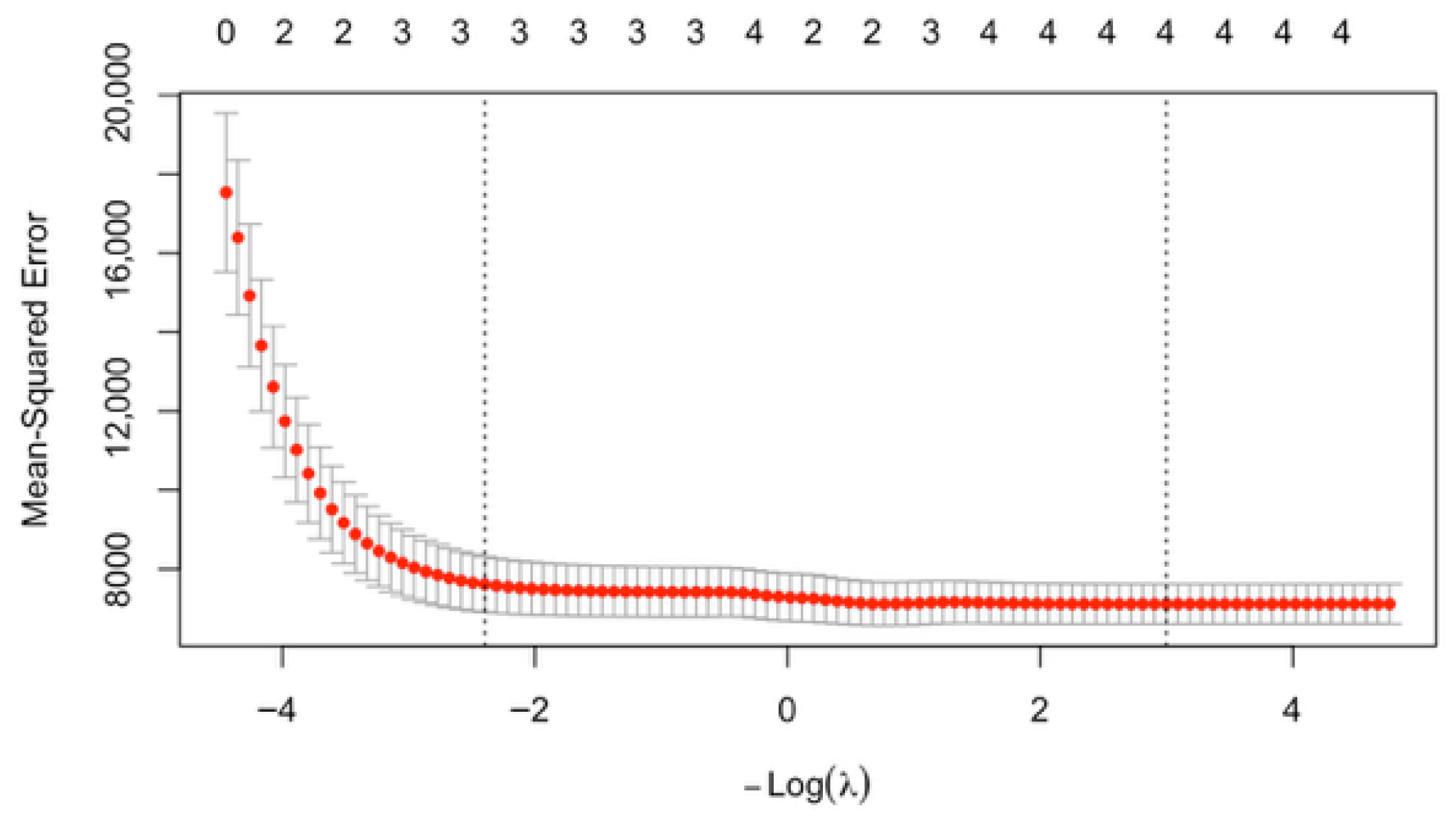
To visualize our relaxed LASSO model, we generated a cross-validation plot showing how predictive error changes across different levels of penalization, represented by the penalty parameter λ (plotted as −log(λ)) (Figure 10 and Figure 11). The x-axis represents the strength of the penalty, with larger values corresponding to more substantial shrinkage. At the same time, the y-axis shows the cross-validated prediction error, measured as mean squared error. This plot illustrates how the model’s complexity varies with λ: larger values produce simpler models with more coefficients shrunk to zero, whereas smaller values produce more complex models with more variables retained (Lockhart et al., 2014). For the MA dataset, the minimum-error model included 6 variables, whereas for the NYC dataset, it included 4 variables. The coefficients of determination and R2 at the best model were reported in Appendix C.
Figure 10.
Cross-validated MSE of LASSO fit and selection of the number of optimal variables in the MA dataset. The first dotted line closest to the y-axis is the lambda (λ) that is within 1 standard error of the minimum mean square error. The second dotted line corresponds to the λ that yields the lowest mean squared error.
Figure 11.
Cross-validated MSE of LASSO fit and selection of the number of optimal variables (LASSO) in the NYC dataset. The first dotted line closest to the y-axis is the lambda (λ) that is within 1 standard error of the minimum mean square error. The second dotted line corresponds to the λ that yields the lowest mean squared error.
3.2.3. Decision Tree
We also used a decision tree, a nonlinear machine learning model that separates data into subgroups based on predictor values. At each node, the algorithm evaluates all candidate predictors. It identifies the variable and threshold that minimizes the prediction error (measured by metrics such as residual sum of squares for regression trees). The selected split produces two child nodes that are more homogeneous with respect to the response variable than the parent node. This process continues iteratively, generating a tree structure composed of decision rules of the form “if condition A, then outcome B.” (Loh & Vanichsetakul, 1988).
Unlike regression models, which assume a linear relationship between predictors and the outcome variable, decision trees capture nonlinearities and interaction effects. For example, in this study, the algorithm may first split schools by the percentage of economically disadvantaged students, then further separate each branch by demographic or college attendance rates. Notably, the same predictor can be used at multiple nodes, each with a different threshold, allowing the tree to model complex relationships across variables. For both the MA and NYC datasets, the decision tree generated graphical tree diagrams, where each split corresponded to a demographic or socio-economic factor, and each terminal node provided a predicted average SAT score for schools within that subgroup. This approach offers interpretable “if–then” rules for predicting school-level SAT scores, highlighting the most influential factors in shaping score disparities. The decision tree provides a straightforward, interpretable approach to predicting a school’s SAT score from its demographic factors, making it a practical, intuitive tool for policymakers (Ripley, 2007).
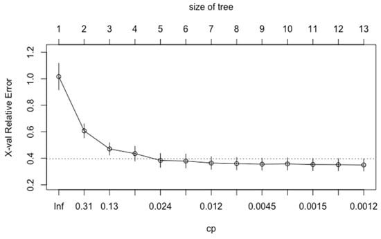
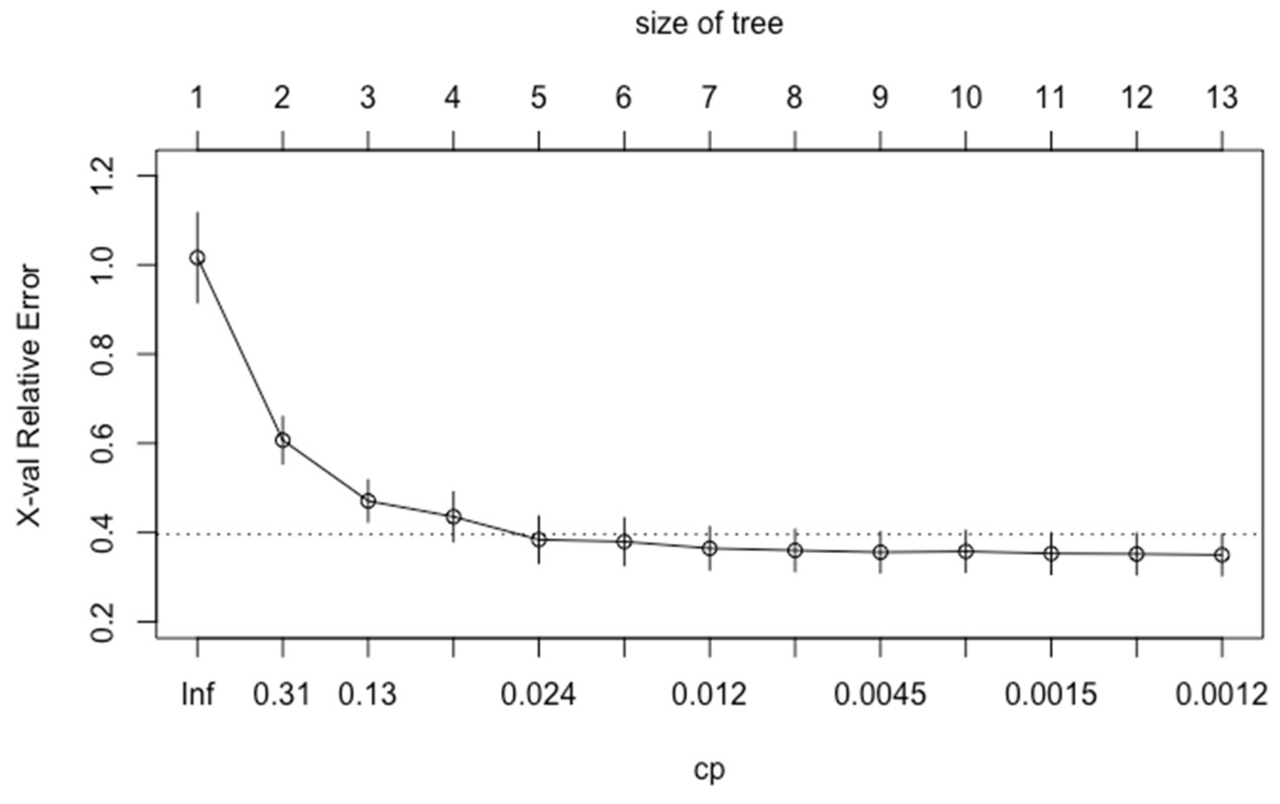
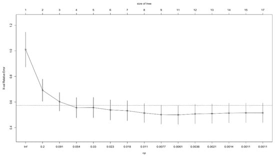
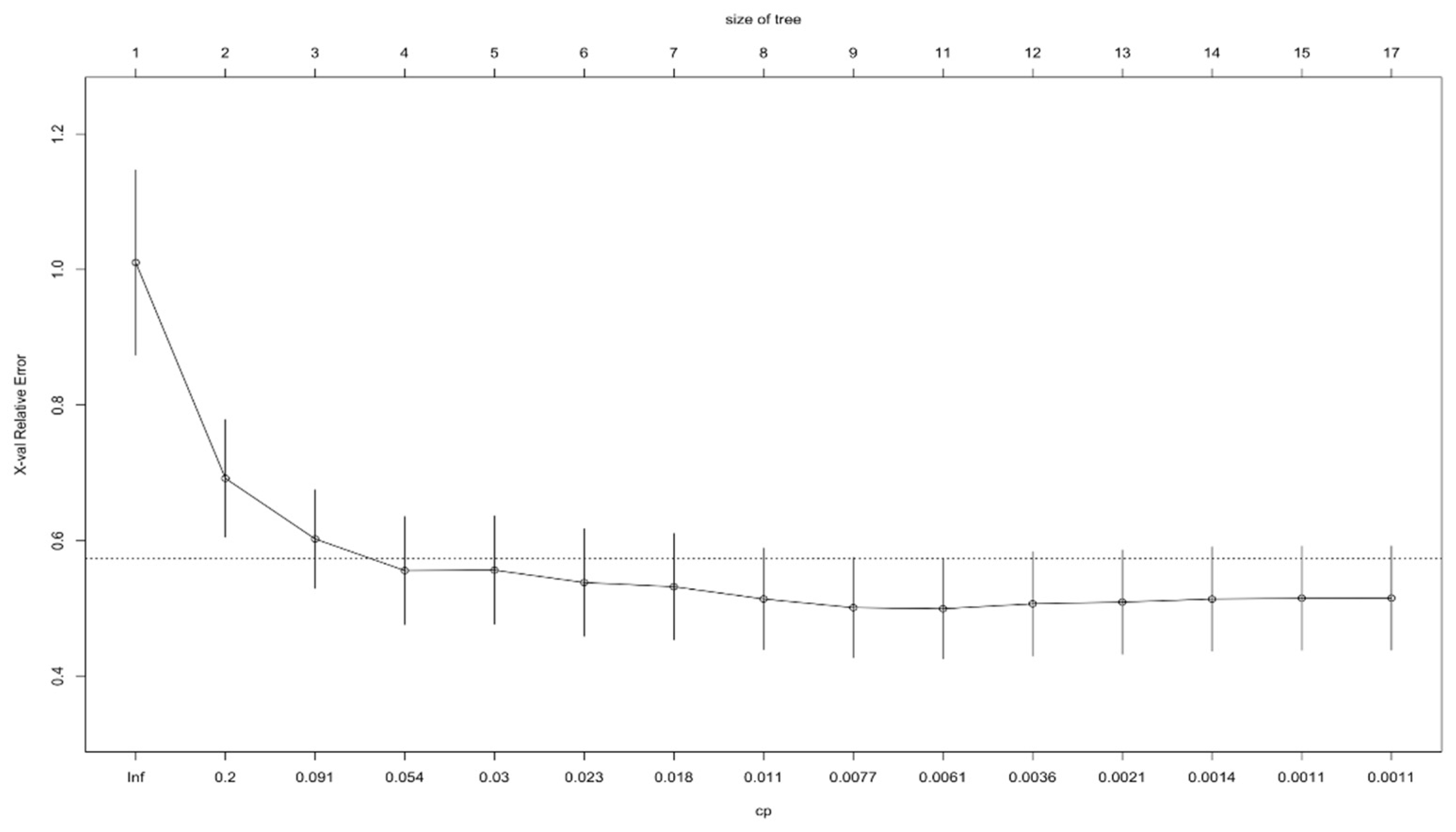
A grid search was implemented to tune the decision tree hyperparameters and mitigate overfitting. The pruning complexity parameter (cp) plots, which illustrate the relative cross-validation error (y-axis) across various cp values (lower x-axis), were shown in Figure 12 (Massachusetts) and Figure 13 (NYC). Smaller cp values correspond to larger trees (upper x-axis). Following Breiman’s one(-standard-error (1-SE) rule (Breiman, 1984), which recommends selecting the smallest tree within one standard error of the minimum cv error, an optimal model with 8–10 terminal nodes was identified for both datasets. The corresponding optimal hyperparameter settings were reported in Appendix D.
Figure 12.
Pruning complexity parameter (cp) plot in MA data. The y-axis is the relative cross-validation (CV) error, the lower x-axis is the complexity parameter (cp) value, the upper x-axis is the number of terminal nodes, and the dashed line represents 1 standard error (SE) of the minimum CV error.
Figure 13.
Pruning complexity parameter (cp) plot in NYC data. The y-axis is the relative cross-validation (CV) error, the lower x-axis is the complexity parameter (cp) value, the upper x-axis is the number of terminal nodes, and the dashed line represents 1 standard error (SE) of the minimum CV error.
4. Results
4.1. Multiple Linear Regression
We used multiple linear regression on both the MA and NYC datasets. For MA data, the model (Table 1) demonstrated that the percent of economically disadvantaged students, the percent of students from racial groups (i.e., Asian, Hispanic, African American, White), and the percent of college matriculation were significant at the 0.001 level. The percentages of economically disadvantaged individuals and of individuals from all racial groups showed negative correlations with the SAT score. The percentage of Asians had the least negative correlation, whereas the percentage of African Americans had the most significant negative correlation. The percentage of students attending college had a positive correlation.
Table 1.
Variables correlated to SAT scores in Massachusetts Public Schools and NYC Public Schools using the Relaxed LASSO approach.
For the NYC dataset, the MLR (Table 1) showed that all variables were statistically significant at the 0.001 level. These variables included the percentage of students from specific racial groups (e.g., White, African American, Hispanic, Asian). All races were negatively correlated with SAT scores, with the percentage of Hispanic students showing the highest negative correlation and the percentage of Asian students showing the lowest.
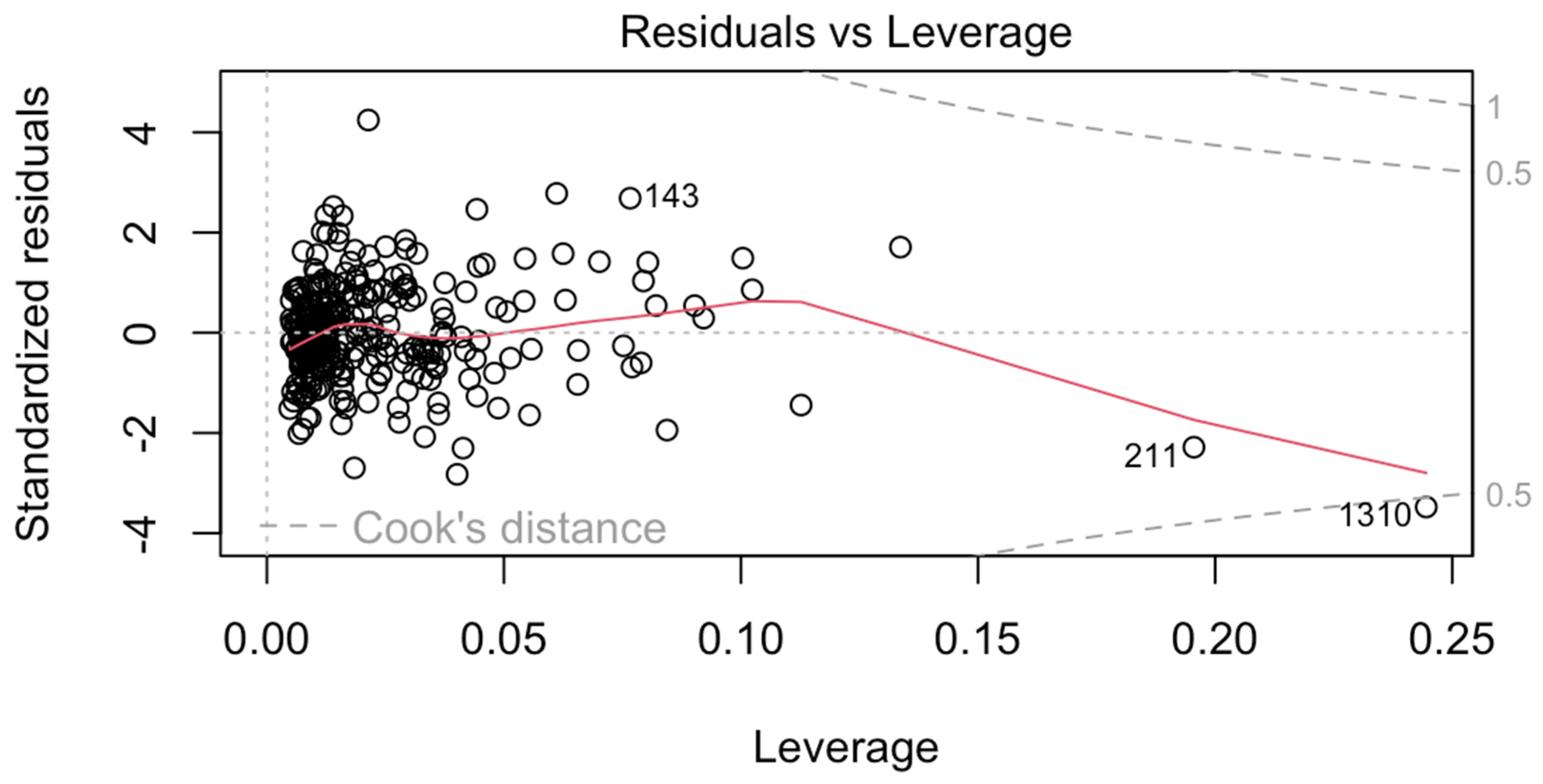
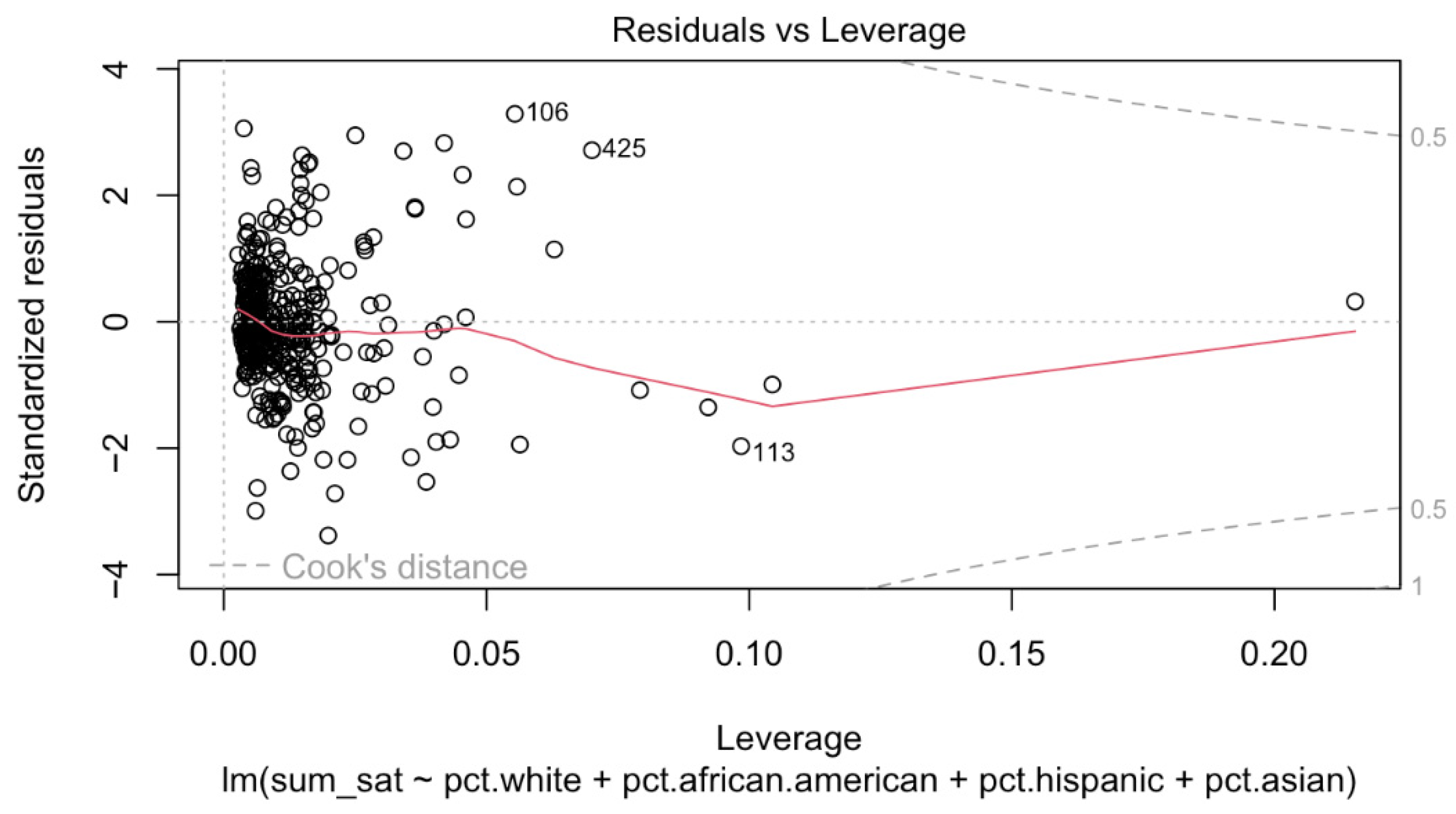
Influence diagnostics based on residuals versus leverage revealed no influential observations in either dataset, as all cases fell well within Cook’s distance thresholds (Appendix B). In contrast, variance inflation factor (VIF) estimates for racial composition variables substantially exceeded conventional thresholds (VIF > 5), indicating severe multicollinearity (Belsley et al., 1980). This result is expected given the compositional structure of the data, in which racial percentages necessarily sum to approximately 100%, inherently inducing strong interdependence among racial groups. Accordingly, MLR was used primarily as an exploratory tool to characterize overall association patterns, while relaxed LASSO—better suited for handling correlated factors—was applied subsequently to assess the stability of these relationships under regularization.
4.2. LASSO Results
As shown in Table 1, the relaxed LASSO regression identified 6 significant variables associated with school-level SAT performance in Massachusetts: the percentage of economically disadvantaged students, the percentage of students from specific racial groups (Asian, Hispanic, African American, and White), and the percentage of students attending college. All racial composition variables were negatively associated with average SAT scores, with the percentage of Asian students showing the weakest negative association and the percentage of African American students showing the strongest negative association. The percentage attending college was positively correlated with SAT performance, while the percentage of economically disadvantaged individuals was negatively correlated.
In the NYC dataset, the relaxed LASSO selected all four racial composition variables (Table 1). Each was negatively correlated with SAT scores, with the percentage of Asians showing the least negative correlation and the percentage of Hispanics the most.
Comparison of results across multiple linear regression and relaxed LASSO revealed highly consistent patterns in the direction and relative magnitude of associations. Despite substantial differences in demographic composition between Massachusetts and New York City, the results consistently showed weaker negative associations for Asian student representation and stronger negative associations for Hispanic and African American students. Similar coefficient estimates and model fit statistics across methods further support the robustness of these findings.
4.3. Decision Tree Analysis
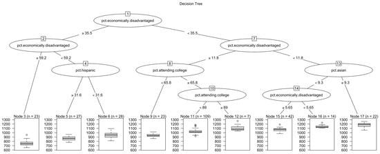
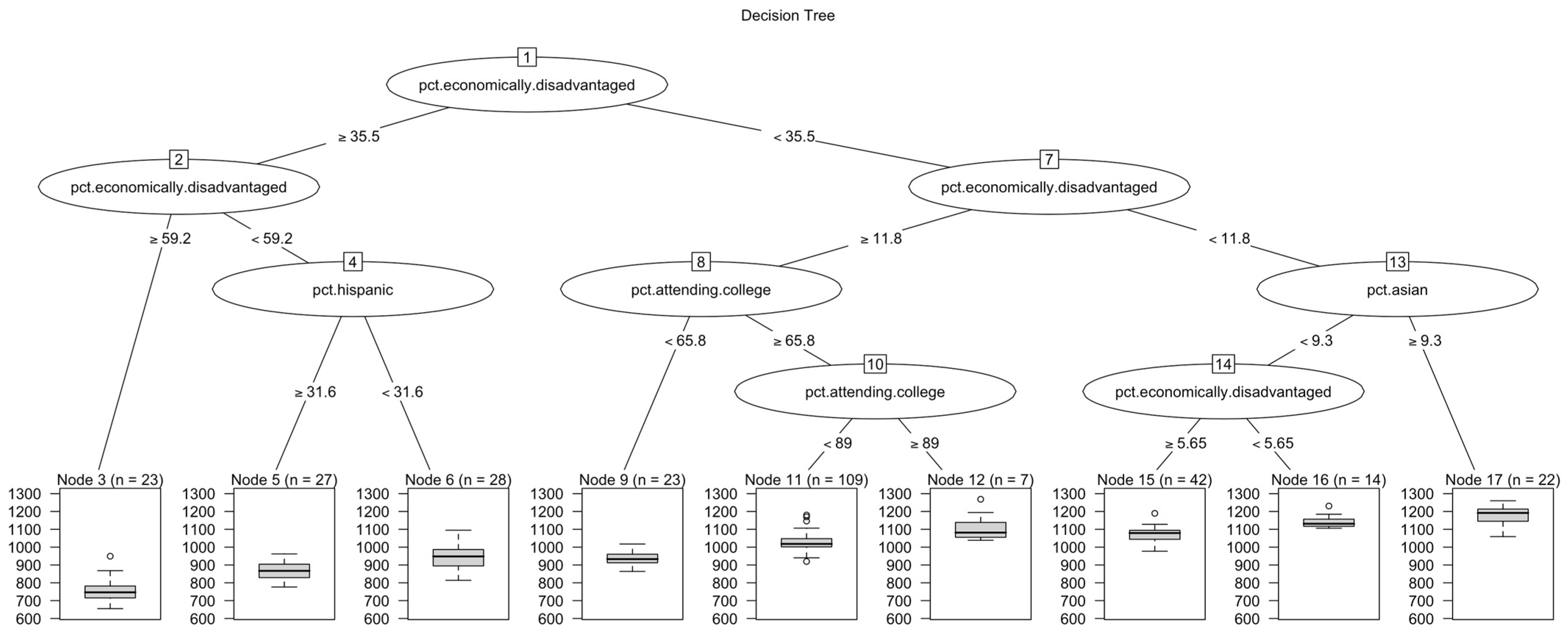
In Massachusetts, the decision tree analysis further illuminated the hierarchical structure of factors associated with school-level SAT performance (Figure 14). The first and most important split was based on the percentage of economically disadvantaged students, indicating that socioeconomic status is the most strongly correlated factor with SAT outcomes.
Figure 14.
The decision tree model of SAT scores and predictors in the MA dataset.
Schools with ≥35.5% economically disadvantaged students consistently had lower average SAT scores, while those with lower proportions performed more competitively. Within the high-poverty group, further splits occurred on % economically disadvantaged (at 59.2%) and subsequently on % Hispanic (at 31.6%). This indicates that, among schools already serving predominantly low-income populations, racial composition has additional influence; schools with higher percentages of Hispanic students had lower SAT scores. For schools with <35.5% disadvantaged students, the next major split was again by % economically disadvantaged (11.8%), highlighting that even moderate differences in poverty levels create meaningful score gaps. Within this branch, splits on college matriculation rates (65.8% and 89%) revealed that schools sending higher proportions of graduates to college have higher SAT averages.
At schools with <11.8% disadvantaged, the model split on % Asian students (at 9.3%), suggesting that at schools with more well-off students, racial composition has a positive effect on SAT scores. Schools with higher percentages of Asian students had the highest predicted average SAT scores in the dataset.
This MA decision tree highlights three main findings. First, economic disadvantage is the highly correlated factor of SAT score, appearing repeatedly at multiple thresholds. Second, race functions as a secondary, conditional factor. For example, the percentage of Hispanic students is featured within high-poverty schools, while the percentage of Asian students is featured within low-poverty schools. Third, school culture, as defined by college attendance rates, is a strong factor in schools with a moderate proportion of low-income students. Together, these patterns indicate that a student’s economic status at a school accounts for most score disparities, while race and college-going culture refine those outcomes.
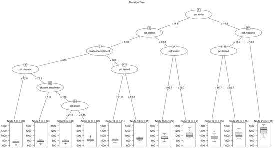
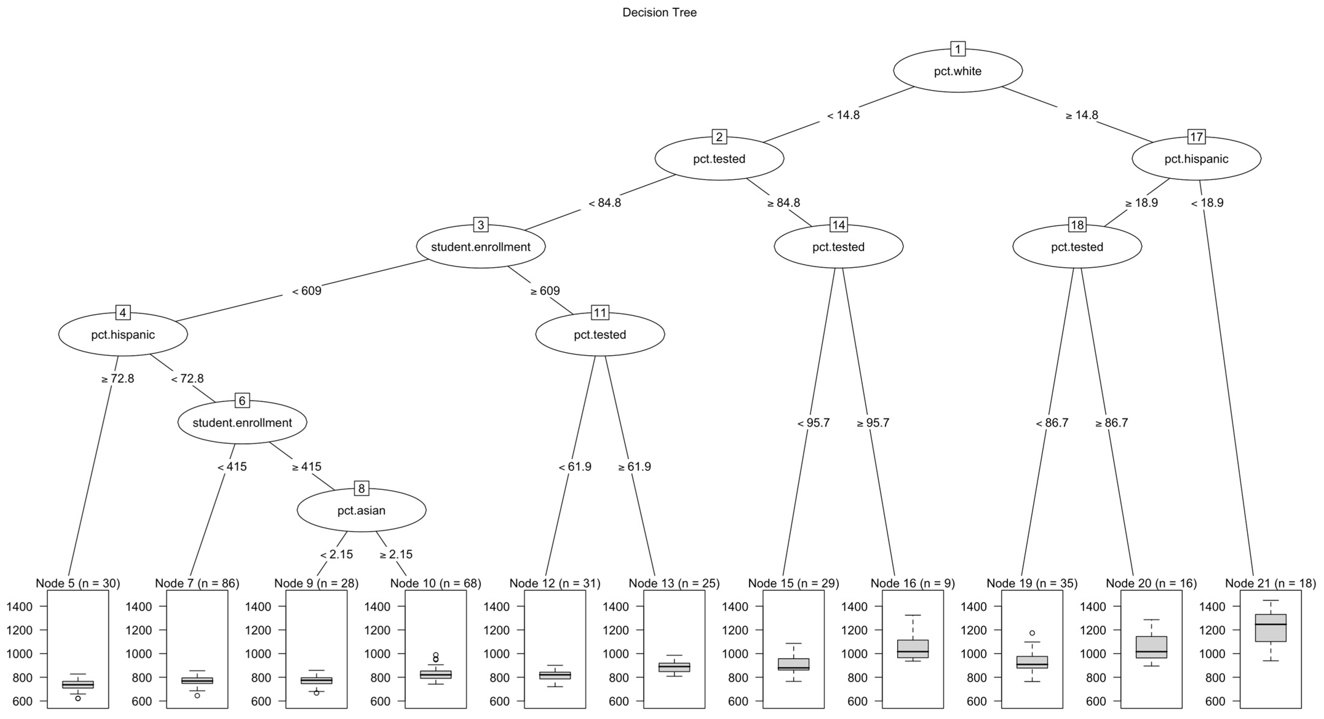
The decision tree for NYC was based solely on racial composition (Figure 15). The first split was based on the percentage of White individuals (14.8%), suggesting that the White demographic is the most important feature associated with SAT scores. Schools with fewer than 14.8% White students generally scored lower, while schools with a higher percentage of White students performed better.
Figure 15.
The decision tree model of SAT scores and predictors in the NYC dataset.
Within the low-White branch (<14.8%), the tree is further split by percent Asian (18.8%). Schools with very low Asian representation (<2.5%) scored the lowest overall, while those with moderate Asian representation (≥2.5%) performed better, especially when combined with low Hispanic enrollment (<9.1%).
Within the high-White branch (≥14.8%), the model next split on the percentage of Hispanic individuals (18.9%). Schools with higher Hispanic enrollment scores tended to score lower, while those with lower Hispanic enrollment scores tended to score higher. Among schools with lower Hispanic enrollment, the final split was again based on the percentage of White students (26.2%), with higher White representation associated with the highest predicted SAT averages.
Although the NYC decision tree produced clear splits by racial composition (percentage of Whites, Hispanics, and Asians), these results should be interpreted cautiously. Unlike the Massachusetts dataset, the NYC dataset lacked socioeconomic and cultural variables, such as the percentage of economically disadvantaged residents and the percentage attending college. So, although the NYC decision tree reflects racial patterns, it is less informative.
5. Discussion
This study employed multiple complementary statistical methods to examine school-level associations between compositional factors such as demographic and socioeconomic distributions and contextual characteristics, including academic preparation, with average SAT performance, using aggregated data from Massachusetts and New York City. Given substantial multicollinearity among key factors, particularly between socioeconomic status and racial composition variables, a sequential modeling strategy integrating multiple linear regression (MLR), the relaxed least absolute shrinkage and selection operator (LASSO), and decision tree analyses was used to identify robust and stable patterns.
Multiple linear regression was first used to characterize broad association trends rather than to estimate isolated marginal effects. Relaxed LASSO was subsequently employed for variable selection and coefficient regularization, thereby improving model stability under multicollinearity. The consistency between MLR and LASSO results strengthened confidence in the robustness of the observed relationships. Because LASSO may arbitrarily select among highly correlated factors, decision tree models were incorporated as a final step to capture hierarchical and nonlinear associations while remaining less sensitive to multicollinearity and independent of linear additivity assumptions.
Across all methods, consistent school-level correlations emerged linking average SAT performance with the school’s socioeconomic composition, racial distribution, and academic preparation. The percentage of economically disadvantaged students exhibited the strongest and most robust negative association with average SAT scores and was consistently identified as the primary factor in MLR, LASSO, and decision tree models. Although economic disadvantage was highly correlated with the proportions of Hispanic and African American students, these racial composition variables were independently selected in both MLR and LASSO and demonstrated stronger negative associations than Asian and White student proportions. Due to the compositional structure of racial variables, near-perfect multicollinearity produced negative coefficients across all racial groups and inflated intercepts; nonetheless, the relative patterns were highly consistent across methods and regions. In both Massachusetts and New York City, Asian and White student proportions showed the weakest negative associations, whereas Hispanic and African American proportions showed stronger negative associations, suggesting more stable relationships across distinct demographic contexts.
Academic preparation, measured by the percentage of students attending college, was also positively associated with SAT performance across models, indicating that schools with stronger college-going cultures tend to achieve higher average scores.
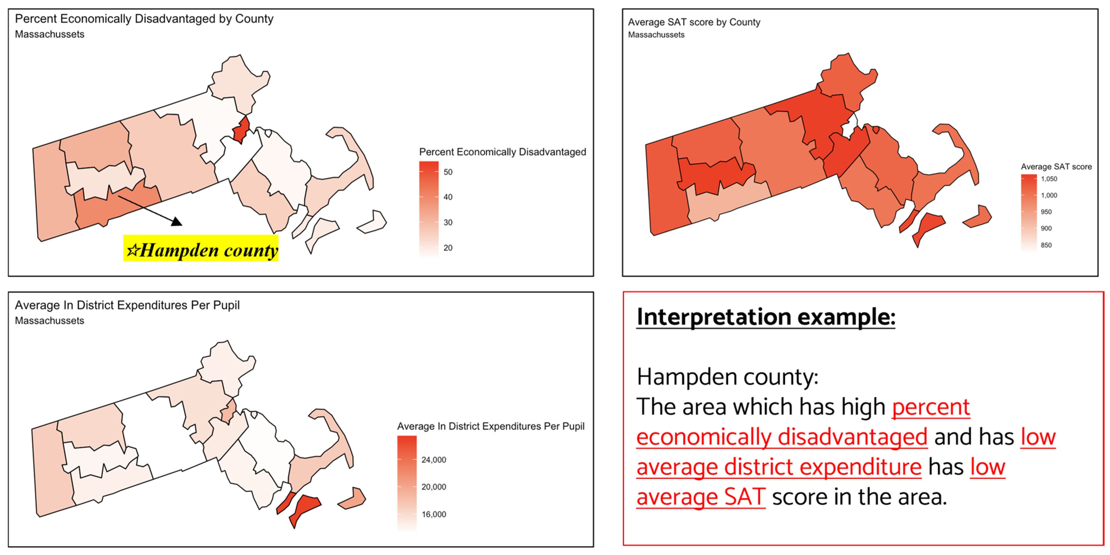
To further assess the robustness of these findings, heat map analyses were conducted for Massachusetts. Counties with higher proportions of economically disadvantaged students consistently exhibit lower average SAT scores, as seen in Hampden County. Additionally, schools with lower SAT performance generally had lower per-pupil expenditures, a trend observed across nearly all counties except Boston (Figure 16), where distinct funding structures and demographic dynamics may be at play.
Figure 16.
SAT scores are associated with economic disadvantages and school expenditure, as shown in a heat map analysis.
6. Study Limitation
6.1. Dataset Limitations
All analyses in this study are conducted using aggregated school-level data, relating average SAT scores to average demographic and socioeconomic characteristics. Because the unit of analysis is the school rather than the individual student, hierarchical linear modeling was not feasible; under these data constraints, multilevel models would reduce mathematically to single-level school models, offering no additional inferential advantage.
The use of aggregated data introduces the risk of ecological fallacy (Robinson, 1950), whereby school-level associations may differ in magnitude or direction from individual-level relationships. Accordingly, observed associations such as the negative relationship between a school’s proportion of economically disadvantaged students and its average SAT score should not be interpreted as evidence of individual-level effects. The study’s findings are therefore limited to between-school patterns, contributing to an understanding of how SAT performance varies across schools with differing demographic and socioeconomic profiles.
Additional limitations arise from dataset asymmetry. The absence of socioeconomic and college-attendance variables in the NYC data limits both interpretation and cross-regional comparability. Nonetheless, the consistency of racial composition patterns observed across Massachusetts and New York City, despite their distinct population structures, provides complementary descriptive evidence supporting the overall findings.
The datasets analyzed were collected in 2014–2015 (New York City) and 2017 (Massachusetts) and obtained from Kaggle. Although there is a gap between data collection and the current study, the analysis focuses on school-level aggregated data and structural educational and socioeconomic variables that are typically stable over time. As a result, this temporal limitation does not undermine the analysis’s relevance to understanding persistent patterns of interest to today’s educators and policymakers.
6.2. Limits of Causal Inference
The analyses presented here rely on cross-sectional, school-level data and therefore do not support causal inference. Because exposure variables (e.g., socioeconomic disadvantage, racial composition, and college-going rates) and outcomes (average SAT scores) are measured simultaneously, temporal precedence cannot be established (Murnane & Willett, 2011). All identified relationships in this study were interpreted as statistical associations.
In particular, variables selected by regression, regularization, and decision tree models reflect explanatory relevance within the observed data rather than causal influence. For example, the association between economic disadvantages and lower average SAT scores does not imply that reducing disadvantage alone would directly raise scores in the absence of broader structural changes. Similarly, the associations between racial composition and SAT performance should not be understood as evidence of direct racial effects. Decision tree splits identify statistical thresholds that optimize data partitioning rather than causal tipping points. Accordingly, these models describe how SAT performance varies across schools with differing demographic and economic profiles, rather than predicting responses to hypothetical interventions.
Despite these limitations, correlational analyses remain valuable for identifying robust, policy-relevant patterns. The convergence of findings across linear, regularized, and nonlinear methods strengthens confidence in the stability of observed relationships and supports broad, evidence-based policy discussions, such as prioritizing resources for schools serving higher proportions of economically disadvantaged students.
7. Implications and Policy Recommendations
The decision tree models identified socioeconomic disadvantage as the dominant school-level correlation of SAT performance, ahead of racial composition and academic preparation. This finding closely aligns with the central conclusions of the Coleman Report (Coleman, 1966/2007), which established that family background characteristics, including parental education, income, and social capital, account for a larger share of variation in academic achievement than differences in school resources alone. In this context, the present results reflect the cumulative effects of unequal educational opportunities across schools, rather than short-term academic differences, and extend Coleman’s core insight to standardized college admissions testing.
At the same time, the observed association between academic preparation (as measured by college-going rates) and SAT performance warrants more explicit theoretical interpretation. A strong college-going culture may operate through multiple pathways. First, it may exert direct peer effects, shaping student motivation, academic norms, and expectations about postsecondary education, which in turn influence engagement with college preparatory coursework and standardized testing. Second, college-going culture likely correlates with school characteristics such as curriculum rigor, availability of advanced coursework, guidance counseling capacity, and teacher experience. In this sense, college-going rates may function as a reinforcing mechanism that amplifies existing disparities. These pathways are consistent with sociological theories of cultural capital (Bourdieu, 1986), in which familiarity with dominant academic norms and expectations confers advantages that are unevenly distributed across schools.
Importantly, “independent” racial composition coefficients after accounting for socioeconomic disadvantage are not evidence of inherent or direct “racial effects” on SAT performance. Rather, these coefficients likely capture a constellation of unmeasured and structurally patterned influences. These could include family- and community-level factors not fully captured by school-level economic disadvantage measures, differential allocation of educational resources across racially segregated districts, cumulative exposure to unequal schooling conditions, and psychosocial mechanisms such as racial paranoia that may affect test performance. From a structural racism framework, race operates as a social and institutional marker that reflects historically produced inequalities in housing, school funding, and access to educational opportunity, rather than a causal attribute of students themselves. Thus, the persistence of race-associated patterns across schools underscores the durability of these structural processes rather than suggesting individual-level racial effects.
The Boston exception in the funding–performance relationship, as illustrated in Figure 16, further highlights the importance of contextual factor under particular conditions. Despite relatively high per-pupil expenditures, Boston schools exhibit lower average SAT scores than would be predicted based on funding alone. This pattern suggests that financial inputs may interact with student need, service provision, and demographic composition in complex ways. In high-need urban districts, increased funding may be directed toward remedial instruction, special education, language support services, or social services that are essential for equity but do not immediately translate into higher standardized test scores. Rather than undermining the importance of school funding, this exception points to the necessity of theorizing how resources are deployed and under what conditions they influence measured academic outcomes.
Taken together, these findings suggest that disparities in SAT performance are best understood as the product of long-standing and cumulative inequities in K–12 educational opportunity, reinforced through interacting mechanisms of socioeconomic disadvantage and contextual mechanisms, including peer composition (Sacerdote, 2001), curriculum tracking (Gamoran, 1987), access to advanced coursework (Klopfenstein, 2004), and school-level college-going culture (McDonough, 1997).
Accordingly, efforts to reduce observed disparities should extend beyond test-specific interventions and instead prioritize policies that address structural inequities in educational access and quality. While targeted SAT preparation programs may provide marginal benefits, they are unlikely to substantially narrow score gaps in the absence of broader reforms (Briggs, 2001; Hardison & Sackett, 2008).
A growing body of empirical evidence points to several policy strategies with demonstrated potential to improve educational outcomes and reduce inequality:
- Sustained tutoring and instructional support, particularly when aligned with grade-level curricula, have been shown to yield substantial gains in academic achievement, especially for low-income students (Cook et al., 2014; Fryer, 2017; Nickow et al., 2020).
- High-quality early childhood education, which produces durable improvements in cognitive development, academic performance, and long-term socioeconomic outcomes for disadvantaged students (Schweinhart et al., 2005; Heckman et al., 2010; Chetty et al., 2011; Duncan & Magnuson, 2013).
- Progressive and sustained school funding in low-income school districts that reduce disparities in instructional resources, class sizes, teacher quality, and access to advanced coursework (Jackson et al., 2016; Lafortune et al., 2018).
- Policies aimed at reducing school segregation, which remains a central mechanism through which socioeconomic and racial inequalities are reproduced across educational institutions (Reardon & Owens, 2014; Rucker & Alexander, 2019).
- Comprehensive community school models, which integrate academic instruction with health, social, and family support services to address non-academic barriers to learning (Maier et al., 2017).
Collectively, these approaches emphasize that meaningful reductions in SAT score disparities require sustained investments in educational equity across the full developmental trajectory, rather than narrowly focused interventions at the point of college admissions. By situating standardized test outcomes within broader structural contexts, these findings support policy frameworks that prioritize expanding opportunities, redistributing resources, and early intervention as central mechanisms for promoting educational equity.
8. Conclusions
Using aggregated school-level data from Massachusetts and New York City (NYC), this study examines the quantitative relationships between average SAT scores and school-level demographics, academic preparation, and funding to inform education policy and equity efforts. Multiple linear regression, relaxed LASSO, and decision tree models were applied as complementary analytical tools. Across all three methods, a consistent pattern emerged: socioeconomic disadvantage showed the strongest and most robust association with lower SAT performance, while racial composition and academic preparation (measured by college-going rates) served as secondary correlates.
Across both regions, schools with higher proportions of Black, Hispanic, and low-income students tended to have lower average SAT scores, whereas schools with higher proportions of White, Asian, and economically advantaged students had higher average SAT scores. Moreover, higher college attendance rates and greater school funding were consistently associated with higher average SAT scores.
These findings represent school-level correlations rather than causal effects and indicate that SAT disparities are closely intertwined with broader structural inequities embedded within the K–12 education system. Accordingly, while targeted SAT preparation initiatives may offer modest benefits, meaningful reductions in observed disparities likely require broader policy interventions to expand equitable access to educational opportunities.
9. Future Work
Future research could benefit from incorporating richer contextual variables into the Massachusetts dataset, including measures of instructional quality, access to tutoring, teacher experience, and curriculum rigor. These additions would allow for a more detailed investigation of the observed Boston anomaly, in which high per-pupil funding coincides with comparatively low average SAT performance, and may help disentangle the institutional and demographic mechanisms underlying this pattern.
For New York City, expanding data availability to include socioeconomic and academic preparation variables comparable to those in the Massachusetts dataset would enable more rigorous cross-regional comparisons and improve the generalizability of findings. Harmonizing variable definitions and measurement frameworks across regions would further facilitate robust comparative analyses.
Because the present study relies on aggregated school-level data, it cannot distinguish within-school variation from between-school differences or separate individual-level processes from institutional dynamics. Future studies incorporating student-level data within hierarchical or mixed-effects modeling frameworks would enable multilevel variance decomposition and provide more precise insights into the mechanisms driving observed disparities.
Finally, the use of longitudinal data and quasi-experimental research designs would allow for establishing temporal ordering and more rigorous evaluation of potential causal pathways. Such approaches would strengthen causal inference and support the development of evidence-based policy interventions grounded in dynamic educational processes.
Author Contributions
Conceptualization, M.L. and W.L.; methodology, M.L. and W.L.; software, M.L.; validation, M.L.; formal analysis, M.L.; investigation, M.L.; resources, M.L. and W.L.; data curation, M.L.; writing—original draft preparation, M.L.; writing—review and editing, M.L. and W.L.; visualization, M.L.; supervision, W.L.; project administration, W.L. All authors have read and agreed to the published version of the manuscript.
Funding
This research received no external funding.
Institutional Review Board Statement
Ethical review and approval were waived for this study because it involved the secondary analysis of publicly available data obtained from Kaggle. The dataset used in this research is open-access, contains no direct or indirect personal identifiers, and is fully de-identified. The authors did not recruit participants, interact with human subjects, or collect any new private or sensitive information. As such, this study does not constitute human subjects research under applicable institutional and federal guidelines, and IRB review was not required.
Informed Consent Statement
Informed consent was waived because the research used open-access data downloaded from Kaggle that are fully de-identified and contain no personally identifiable information. The study did not involve contact with individuals, and obtaining consent from original data contributors was not practicable given the public, anonymized nature of the dataset.
Data Availability Statement
Data is available upon request via email.
Conflicts of Interest
The authors declare no conflicts of interest.
Appendix A
Table A1.
List of prior studies to examine individual and school-level effects on SAT score gaps.
Appendix B
Documentation for MLR and Evaluation—Equation (A1) (MA data) and Equation (A2) (NYC data).
Appendix B.1. Massachusetts
MA data—MLR Equation (A1)
Figure A1.
MA data—MLR Output.
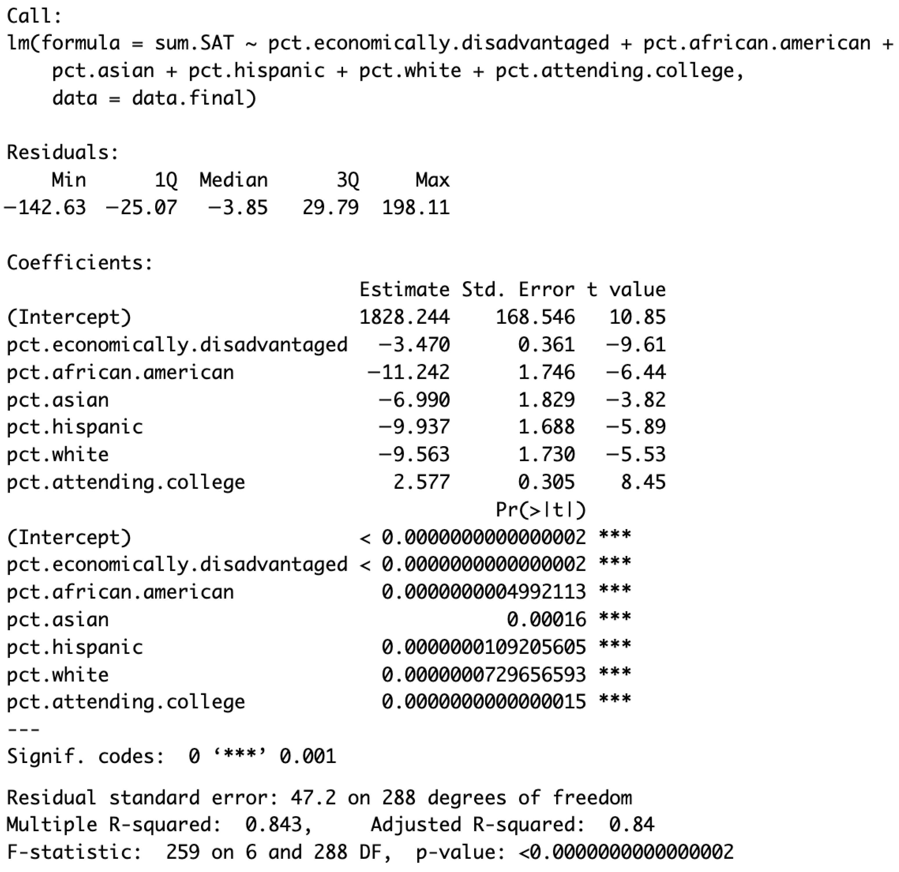
Figure A2.
MA data MLR—VIF (Variance Inflation Factor) Output.
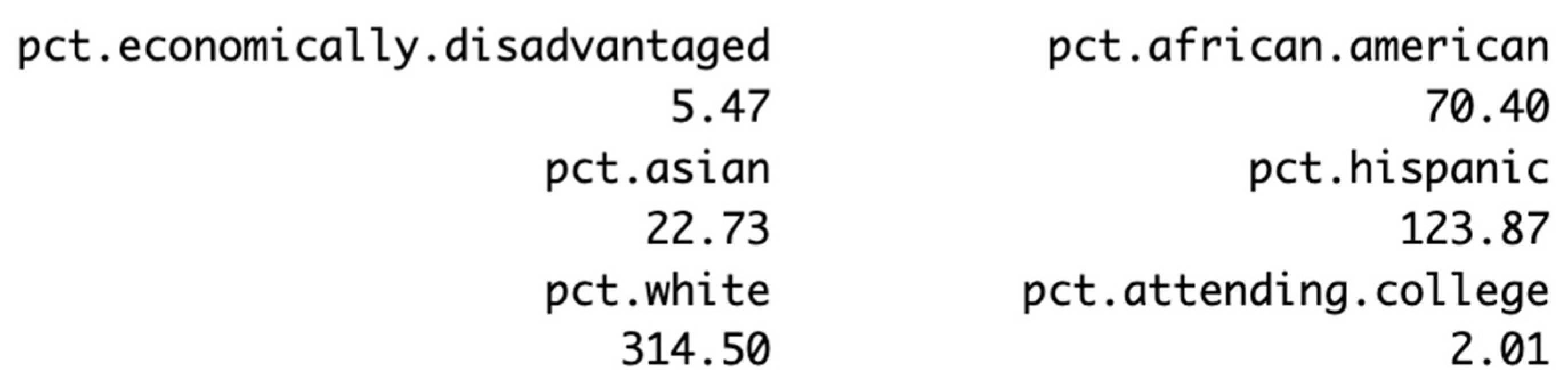
Figure A3.
MA data MLR—Residual vs. Leverage plot for influence diagnostics.
Appendix B.2. NYC
NYC data—MLR Equation (A2)
Figure A4.
NYC data—MLR Output.
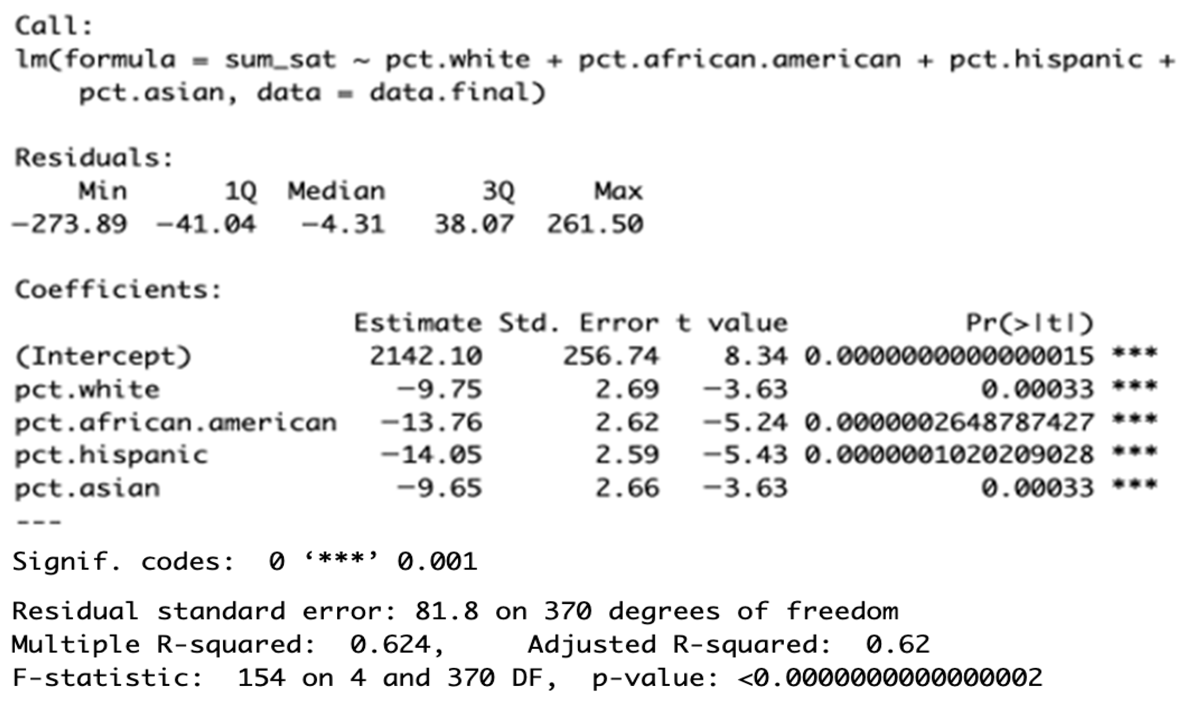
Figure A5.
NYC data MLR—VIF (Variance Inflation Factor) Output.

Figure A6.
NYC data MLR—Residual vs. Leverage plot for influence diagnostics.
Appendix B.3
Table A2.
Evaluation Metrics for MLR Modeling.
Appendix C
Documentation for LASSO Output and Evaluation Metrics Table 1.
Figure A7.
Massachusetts—LASSO Output.
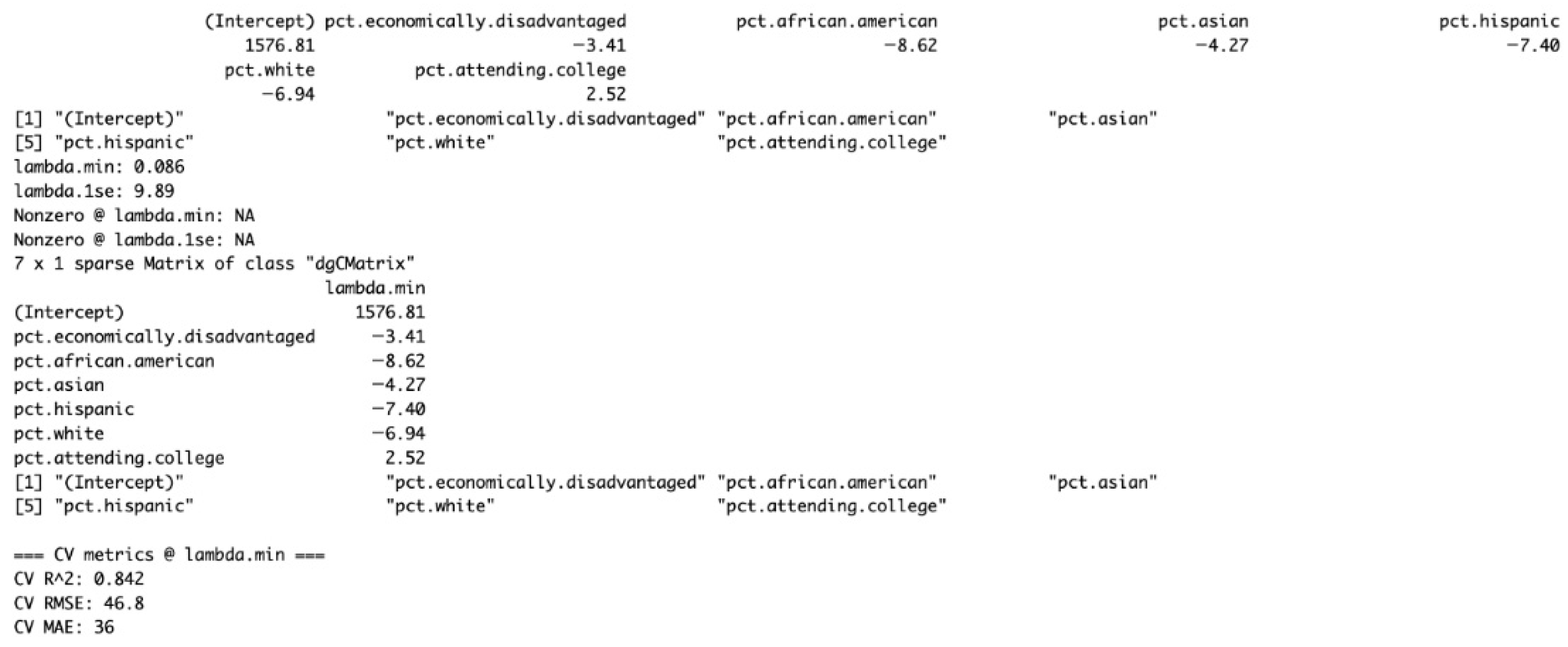
Figure A8.
NYC—LASSO Output.
Appendix D
Documentation for Decision Tree Evaluation Metrics.
Figure A9.
Massachusetts—Hyperparameters Output for Decision Tree.

Figure A10.
NYC—Hyperparameters Output for Decision Tree.

References
- Atkinson, R. C. (2009, April 13–17). The new SAT: A test at war with itself. Annual meeting of the American Educational Research Association, San Diego, CA, USA. [Google Scholar]
- Belsley, D. A., Kuh, E., & Welsch, R. E. (1980). Regression diagnostics: Identifying influential data and sources of collinearity. Wiley. [Google Scholar]
- Bourdieu, P. (1986). The forms of capital. In J. G. Richardson (Ed.), Handbook of theory and research for the sociology of education (pp. 241–258). Greenwood Press. [Google Scholar]
- Breiman, L. (1984). Classification and regression trees. Routledge. [Google Scholar]
- Briggs, D. C. (2001). The effect of admissions test preparation: Evidence from NELS:88. Chance, 14(1), 10–18. [Google Scholar] [CrossRef] [Scilit]
- Camara, W. J., & Schmidt, A. E. (1999). Group differences in standardized testing and social stratification. (College Board Research Report 1999, No. 99-5). The College Board. [Google Scholar]
- Chetty, R., Deming, D. J., & Friedman, J. N. (2023). Diversifying society’s leaders? The determinants and causal effects of admission to highly selective private colleges. (NBER Working Paper 2023, No. 31492). National Bureau of Economic Research. [Google Scholar]
- Chetty, R., Friedman, J. N., Hilger, N., Saez, E., Schanzenbach, D. W., & Yagan, D. (2011). How does your kindergarten classroom affect your earnings? Evidence from Project Star. The Quarterly Journal of Economics, 126(4), 1593–1660. [Google Scholar] [CrossRef] [Scilit] [PubMed]
- Coleman, J. S. (2007). Equality of educational opportunity (COLEMAN) study (EEOS). Inter-University Consortium for Political and Social Research [distributor]. (Original work published 1966). [Google Scholar] [CrossRef] [Scilit]
- Cook, P. J., Dodge, K., Farkas, G., Fryer, R., Guryan, J., Ludwig, J., Mayer, S., Pollack, H., & Steinberg, L. (2014). The (surprising) efficacy of academic and behavioral intervention with disadvantaged youth: Results from a randomized experiment in Chicago. (NBER Working Paper No. w19862). NBER. Available online: https://ssrn.com/abstract=2386403 (accessed on 24 January 2026).
- Dalziel, N. (2017). Massachusetts public schools data. Kaggle. Available online: https://www.kaggle.com/datasets/ndalziel/massachusetts-public-schools-data (accessed on 24 January 2026).
- Dixon-Román, E. J., Everson, H. T., & McArdle, J. J. (2013). Race, poverty, and SAT scores: Modeling the influences of family income on black and white high school students’ SAT performance. Teachers College Record, 115, 1–33. [Google Scholar] [CrossRef] [Scilit]
- Duncan, G. J., & Magnuson, K. (2013). Investing in preschool programs. Journal of Economic Perspectives, 27(2), 109–132. [Google Scholar] [CrossRef] [Scilit]
- Everson, H. T., & Millsap, R. E. (2004). Beyond individual differences: Exploring school effects on SAT scores. Educational Psychologist, 39, 157–172. [Google Scholar] [CrossRef] [Scilit]
- Fryer, R. G. (2017). The production of human capital in developed countries: Evidence from 196 randomized field experiments. (NBER Working Paper No. 22130). National Bureau of Economic Research. Available online: https://www.nber.org/papers/w22130 (accessed on 24 January 2026).
- Fryer, R. G., & Levitt, S. D. (2004). Understanding the black–white test score gap in the first two years of school. Review of Economics and Statistics, 86, 447–464. [Google Scholar] [CrossRef] [Scilit]
- Gamoran, A. (1987). The stratification of high school learning opportunities. Sociology of Education, 60(3), 135–155. [Google Scholar] [CrossRef] [Scilit]
- Geiser, S. (2015). The growing correlation between race and SAT scores: New findings from California. (Research & Occasional Paper Series: CSHE.10.15). Center for Studies in Higher Education, University of California. [Google Scholar]
- Geiser, S. (2017). Norm-referenced tests and race-blind admissions: The case for eliminating the SAT and ACT at the University of California. (Research & Occasional Paper Series 2017, CSHE.15.17). Center for Studies in Higher Education, University of California. [Google Scholar]
- Hardison, C. M., & Sackett, P. R. (2008). Use of writing samples on standardized tests: Susceptibility to rule-based coaching and the resulting effects on score improvement. Applied Measurement in Education, 21(3), 227–252. [Google Scholar] [CrossRef] [Scilit]
- Heckman, J. J., Moon, S. H., Pinto, R., Savelyev, P. A., & Yavitz, A. (2010). The rate of return to the HighScope Perry Preschool Program. Journal of Public Economics, 94(1–2), 114–128. [Google Scholar] [CrossRef] [Scilit] [PubMed]
- Hiss, W. C., & Franks, V. W. (2014). Defining promise: Optional standardized testing policies in American college and university admissions. National Association for College Admission Counseling (NACAC). [Google Scholar]
- Jackson, C. K., Johnson, R. C., & Persico, C. (2016). The effects of school spending on educational and economic outcomes. Quarterly Journal of Economics, 131(1), 157–218. [Google Scholar] [CrossRef] [Scilit]
- JBHE Foundation. (1998). Why Family Income Differences Don’t Explain the Racial Gap in SAT Scores. The Journal of Blacks in Higher Education, 20, 6–8. [Google Scholar] [CrossRef] [Scilit]
- KFF. (2017). State health facts. Population distribution by race/ethnicity. Available online: https://www.kff.org/state-health-policy-data/state-indicator/distribution-by-raceethnicity/?currentTimeframe=6&sortModel=%7B%22colId%22:%22Location%22,%22sort%22:%22asc%22%7D (accessed on 24 January 2026).
- Kim, B. (2015). Understanding diagnostic plots for linear regression analysis. UVA Library StatLab. Available online: https://library.virginia.edu/data/articles/diagnostic-plots (accessed on 24 January 2026).
- Klopfenstein, K. (2004). Advanced placement: Do minorities have equal opportunity? Economics of Education Review, 23(2), 115–131. [Google Scholar] [CrossRef] [Scilit]
- Kobrin, J. L., Milewski, G. B., Everson, H. T., & Zhou, Y. (2003). An investigation of school-level factors for students with discrepant high school GPA and SAT scores. (ERIC Document Reproduction Service No. ED476921). ERIC. [Google Scholar]
- Lafortune, J., Rothstein, J., & Schanzenbach, D. W. (2018). School finance reform and the distribution of student achievement. American Economic Journal: Applied Economics, 10(2), 1–26. [Google Scholar] [CrossRef] [Scilit]
- Larion, A. (2016). Average SAT scores for NYC public schools. Kaggle. Available online: https://www.kaggle.com/datasets/nycopendata/high-schools (accessed on 24 January 2026).
- Liu, M., Lu, W., & Zhao, L. (2024, March 9). Decoding SAT scores: A multifaceted analysis of socioeconomic and educational influences across diverse regions. IEEE Integrated STEM Education Conference (ISEC 2024) (pp. 1–2), Princeton, NJ, USA. [Google Scholar] [CrossRef] [Scilit]
- Lockhart, R., Taylor, J., & Tibshirani, R. J. (2014). A significance test for the lasso. The Annals of Statistics, 42(2), 413–468. [Google Scholar] [CrossRef] [Scilit]
- Loh, W. Y., & Vanichsetakul, N. (1988). Tree-structured classification via generalized discriminant analysis. Journal of the American Statistical Association, 83(403), 715–725. [Google Scholar] [CrossRef]
- Maier, A., Daniel, J., Oakes, J., & Lam, L. (2017). Community schools as an effective school improvement strategy: A review of the evidence. Learning Policy Institute. [Google Scholar]
- McDonough, P. M. (1997). Choosing colleges: How social class and schools structure opportunity. SUNY Press. [Google Scholar]
- Murnane, R. J., & Willett, J. B. (2011). Methods matter: Improving causal inference in educational and social science research. Oxford University Press. [Google Scholar]
- National Association for College Admission Counseling (NACAC). (2008). Report of the commission on the use of standardized tests in undergraduate admission. NACAC. [Google Scholar]
- Nickow, A., Oreopoulos, P., & Quan, V. (2020). The impressive effects of tutoring on PreK-12 learning: A systematic review and meta-analysis of the experimental evidence. (NBER Working Paper No. 27476). National Bureau of Economic Research. [Google Scholar] [CrossRef] [Scilit]
- R Core Team. (2024). R: A language and environment for statistical computing (Version 4.4.1). R Foundation for Statistical Computing. Available online: https://www.R-project.org/ (accessed on 14 July 2024).
- Reardon, S. F., & Owens, A. (2014). 60 years after Brown: Trends and consequences of school segregation. Annual Review of Sociology, 40, 199–218. [Google Scholar] [CrossRef] [Scilit]
- Ripley, B. D. (2007). Pattern recognition and neural networks. Cambridge University Press. [Google Scholar]
- Robinson, W. S. (1950). Ecological correlations and the behaviour of individuals. American Sociological Review, 15(3), 351–357. [Google Scholar] [CrossRef] [Scilit]
- Rucker, J., & Alexander, N. (2019). Children of the dream: Why school integration works. Basic Books. [Google Scholar]
- Sacerdote, B. (2001). Peer effects with random assignment: Results for Dartmouth roommates. Quarterly Journal of Economics, 116(2), 681–704. [Google Scholar] [CrossRef] [Scilit]
- Sackett, P. R., Kuncel, N. R., Arneson, J. J., Cooper, S. R., & Waters, S. D. (2009a). Does socioeconomic status explain the relationship between admissions tests and postsecondary academic performance? Psychological Bulletin, 135, 1–22. [Google Scholar] [CrossRef] [Scilit]
- Sackett, P. R., Kuncel, N. R., Arneson, J. J., Cooper, S. R., & Waters, S. D. (2009b). Socioeconomic status and the relationship between the SAT® and freshman GPA: An analysis of data from 41 colleges and universities. (College Board Research Report 2009, No. 2009-1). The College Board. [Google Scholar]
- Sackett, P. R., Kuncel, N. R., Beatty, A. S., Rigdon, J. L., Shen, W., & Kiger, T. B. (2012). The role of socioeconomic status in SAT–grade relationships and in college admissions decisions. Psychological Science, 23(9), 1000–1007. [Google Scholar] [CrossRef] [Scilit]
- Schweinhart, L. J., Montie, J., Xiang, Z., Barnett, W. S., Belfield, C. R., & Nores, M. (2005). Lifetime effects: The HighScope perry preschool study through age 40. (Monographs of the HighScope Educational Research Foundation, 14). HighScope Press. [Google Scholar]
- Tibshirani, R. (1996). Regression shrinkage and selection via the lasso. Journal of the Royal Statistical Society: Series B (Methodological), 58, 267–288. [Google Scholar] [CrossRef] [Scilit]
- Zwick, R., & Green, J. G. (2007). New perspectives on the correlation of SAT scores, high school grades, and socioeconomic factors. Journal of Educational Measurement, 44(1), 23–45. [Google Scholar] [CrossRef] [Scilit]
- Zwick, R., & Himelfarb, I. (2011). The effect of high school socioeconomic status on the predictive validity of SAT scores and high school grade-point average. Journal of Educational Measurement, 48(2), 101–121. [Google Scholar] [CrossRef] [Scilit]

Disclaimer/Publisher’s Note: The statements, opinions and data contained in all publications are solely those of the individual author(s) and contributor(s) and not of MDPI and/or the editor(s). MDPI and/or the editor(s) disclaim responsibility for any injury to people or property resulting from any ideas, methods, instructions or products referred to in the content. |
© 2026 by the authors. Licensee MDPI, Basel, Switzerland. This article is an open access article distributed under the terms and conditions of the Creative Commons Attribution (CC BY) license.