


Abstract
This study forecasts inbound tourism demand for the United Kingdom, using monthly data from February 1989 to February 2020. In the empirical analysis, we evaluate and compare the performance of five machine learning models (decision trees, random forests, XGBoost, and support vector regression with the RBF and linear kernels) against a more traditional linear SARIMA regression model. Forecasting performance metrics included MSE, RMSE, MAE, R2, and MAPE. The SVR RBF kernel model achieves the highest accuracy, with an MAPE of 0.014% on the training set. To enhance model interpretability, feature importance analysis is applied to identify the most influential predictors of tourist arrivals. This research offers significant policy implications, aiding government policymakers and private industry stakeholders in optimizing their planning and decisions, deploying better long-term business strategies and tourism-related services, and optimizing the allocation of public and private resources to support the tourism sector.
1. Introduction
Tourism has long been recognized as a major contributor to economic activity through job creation, investment stimulation, increasing foreign exchange reserves, and regional development. Internationally, tourism demand has played a significant role in supporting and boosting national economies. Tourism is a complex industry incorporating social, cultural, political, educational, and economic dimensions. Furthermore, in recent decades, people’s ability to travel has significantly improved due to the rising real disposable income, more efficient and less expansive transport infrastructure, and increased need for international mobility. These factors have contributed to the increased frequency of international travel. These economic and social changes have encouraged and sustained the growth of the tourism industry (Haryanto, 2020). According to the World Tourism Organization (UNWTO), the tourism industry is internationally the third-largest export industry, and in many developing countries, it is the top export category, contributing up to 20% of the Gross Domestic Product.
Globally, in 2025, the tourism sector accounted for $11.7 trillion or 10.3% of world GDP and supported 371 million jobs or 10.9% of total global employment, reflecting the sector’s strong link to rising middle-class income and increased consumer spending (World Travel & Tourism Council, 2025). Specifically for the UK, a study by the Office for National Statistics shows that the travel and tourism industries contributed 6.7% of all gross added value for the United Kingdom in 2018 (ONS, 2020). Given the apparent economic importance of tourism, forecasting tourism demand has become one of the most extensively researched areas in tourism economics. This line of research is significant for planning and investment decisions, marketing strategies, and central or regional public policy.
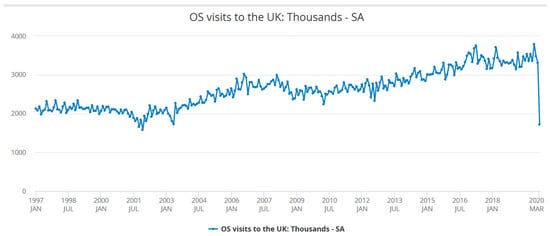
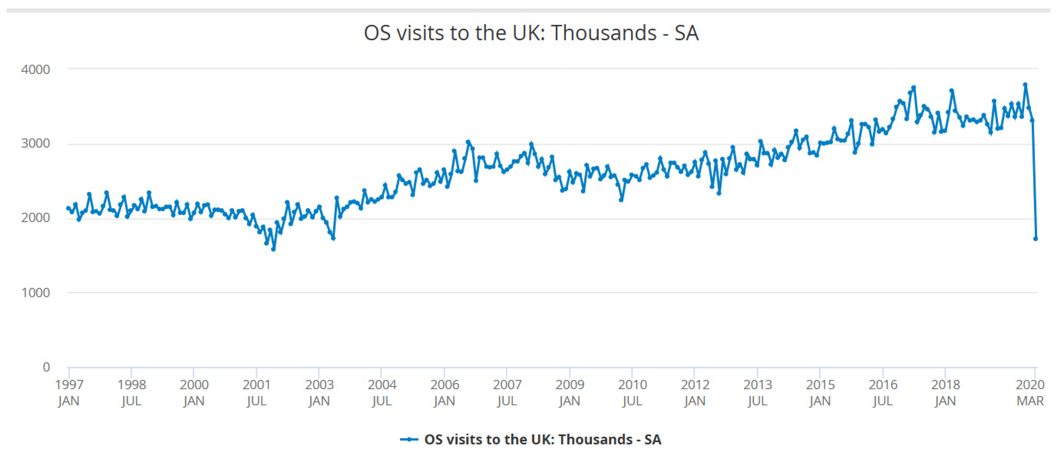
Figure 1 illustrates the seasonally adjusted monthly international inbound visits to the UK. Despite some breakpoints, e.g., July 2001 and January 2009, the data show a clear long-term positive trend in inbound tourism for the UK. Our dataset, which covers more than 20 years and thus includes a series of major global economic events, such as the dot-com crisis and the 2008 global financial crisis, offers a long and rich time frame for analysing tourism demand.
Figure 1.
Seasonally adjusted monthly overseas visits to the UK (in thousands), 1997–2020. Source 1, Office for National Statistics.
Accurate forecasting of tourism demand is essential to government agencies, large tourism operators, and small local businesses, enabling more efficient resource allocation, designing targeted marketing strategies and adequate infrastructure planning and development (Song & Li, 2008; J. Zhang & Gao, 2025; Khatibi et al., 2022; Dimitriadou et al., 2024). The need for reliable forecasts is further enhanced by the fragile nature of tourism and hospitality services, where unused capacity—such as empty hotel rooms or unsold event tickets—cannot be recovered once the sales opportunity has passed, resulting in a permanent loss of the relevant revenue (Song, 2003). In this research, we employ machine learning (ML) models, since they can capture linear and non-linear relationships and complex interactions between the variables, unlike conventional linear econometric time series models. In these ML models, a rich set of independent variables is used that includes domestic economic conditions as described by the Consumer Price Index (CPI) and inflation, the real GDP, exchange rates, and major financial market indicators over the period 1997–2020 (we exclude the period affected by the COVID-19 pandemic). The goal is to see how these variables affect inbound travel to the United Kingdom. The frequency of the data is monthly, and a cross-validation technique with grid search is applied to efficiently tune the ML models’ hyperparameters. With cross-validation, we manage to optimize the bias and variance trade-off and ensure that our optimal model is able to describe the real underlying data-generating mechanism and not noise or sample-specific characteristics.
Within this framework, we make two key contributions to the tourism demand literature: First, we employ a long-term perspective by studying UK tourism demand over three decades, offering insights into the evolving relationship between economic conditions and tourism. Second, we uncover individual links between economic indicators and tourism flows, illustrating the marginal effects of the most influential variables.
The rest of the paper is organized as follows: Section 2 describes the methodologies used in our study. Section 3 provides an overview of our data. Section 4 presents our empirical results. Finally, Section 5 concludes and discusses the implications of our findings.
Literature Review
Machine learning (ML) techniques have been successfully used to forecast tourist demand (TD) in the past, resulting in significantly improved forecasting accuracy. For instance, K.-Y. Chen and Wang (2007) tested the performance of a GA-trained SVR in forecasting tourism demand, by comparing it to Artificial Neural Networks (ANNs) and the Autoregressive Integrated Moving Average (ARIMA) model. Their results revealed the superiority of the GA-SVR model, reaching 2.457% MAPE, over the other methodologies. These results offer evidence that combining evolutionary optimization with SVR can produce consistently accurate forecasts for series with significant seasonality and variability.
Claveria and Torra (2014) forecasted tourist demand by comparing the performance of alternative ANN architectures. Using monthly tourist arrivals to Catalonia by country of origin over the period 2001–2012, they assess forecasting accuracy across different horizons and memory structures. Their findings show that the ANN model performed particularly well over the 12-month forecasting horizon, with a Root Mean Square Error of 1.94. However, in some counties, the Autoregressive Integrated Moving Average (ARIMA) model consistently outperformed across all horizons.
R. Chen et al. (2015) forecast holiday tourist daily flows based on the SVR model coupled with the Adaptive Genetic Algorithm and the Seasonal Index Adjustment (AGA-SSVR). They compared the forecasting performance of their model against benchmark models using standard error metrics. Their findings showed that, compared to standard SVR without adaptive parameter tuning and other conventional forecasting techniques, the AGA-SSVR model achieved significantly higher accuracy in predicting daily tourist flows during the holidays. Similarly, B. Zhang et al. (2017) explicitly address the problem of tourism volume forecasting, which they characterize as a non-linear process. Using monthly tourist arrival data from China, the authors propose a hybrid model that combines the support vector regression (SVR) with the Bat Algorithm (BA) to optimize SVR parameters. Their results demonstrate that the BA-SVR model significantly outperforms traditional benchmark models.
Moreover, deep learning (DL) has been applied in the tourism industry to enhance economic analysis and marketing strategies formulation by leveraging advanced modelling techniques to predict economic impact and visitor behaviour. J. Zhang and Gao (2025) proposed a Tourism Variable Recurrent Neural Network (TourVaRNN) to predict tourism demand, visitor spending patterns and behaviour, and economic impact, enabling more effective marketing strategies through visitor segmentation, prediction of spending patterns, and optimized budget allocation. Their results showed improvements in segmentation efficiency by 15.7%, a reduction in inference time by 17.5% and an increase in budget allocation utilization by 13.4%, supporting real-time decision-making and operational efficiency in tourism management.
Building on these machine learning approaches, recent studies have increasingly adopted deep learning techniques and multi-source data to further enhance tourism demand forecasting accuracy. For example, a recent study conducted by Z. Zhang et al. (2025) suggested a PCA-STL-LSTM model that combined seasonal trend decomposition with multi-source data such as search engine data, weather data, and holiday data, predicting daily tourist arrivals at Jiuzhaigou and Mount Siguniang. The results showed that the model performed better over a variety of forecast horizons than state-of-the-art forecasting models, machine learning techniques, and conventional time series models. More effective tourism management and targeted marketing tactics are supported by this increased forecast accuracy.
Recent advances in tourism demand forecasting have been focused on increasing predictive accuracy during both normal and crisis periods. Liu et al. (2026) presented the BayesBag method combining bootstrap-aggregating and Bayesian forecasting techniques. The authors showed that the suggested approach performed better than the Autoregressive Distributed Lag (ADL) models in both pre-COVID-19 and pandemic periods using monthly tourism data from Europe. The study emphasizes the significance of sentiment-based and psychological indicators in tourism predictions.
Machine learning (ML) algorithms in tourism demand forecasting often face challenges related to data volume. Most conventional ML algorithms, such as neural networks, random forests, and support vector machines, are designed to extract complex non-linear patterns from large datasets. Their predictive strength typically increases with the volume and diversity of training observations (Li & Law, 2020).
However, tourist demand is typically reported at relatively low frequencies, e.g., monthly, quarterly or even annually, limiting the number of available observations. Several studies address this issue by exploring methods to enhance forecasting accuracy despite these limitations. For example, Havranek and Zeynalov (2021) demonstrate that incorporating weekly Google Trends data improves the prediction of monthly tourist arrivals. They show that high-frequency information improves forecast accuracy compared to models based only on monthly data using mixed data sampling (MIDAS) models. This suggests that the limitations of low-frequency tourism demand data can be mitigated by high-frequency variables.
Overfitting and bias-variance compensation are challenges associated with small sample sizes in both machine learning and conventional econometric models. Limited data can cause machine learning models to overfit the training set, capturing noise instead of underlying patterns, which hinders the models’ ability to generalize to new data. Noise, a small training set, and model complexity are the causes of this overfitting (Ying, 2019).
In forecasting, using either ML or traditional econometric models, small datasets often lead to poor forecasting accuracy. ML algorithms, being highly non-linear, if not trained correctly, can overfit the data, especially when they are trained with a small number of observations. They will produce models that fit the in-sample (training) data very well, but their performance in new out-of-sample data will be poor. In relevant terminology, this issue reflects the trade-off between bias and variance of the trained models. Bias refers to the in-sample accuracy of the models, while variance refers to the discrepancy in accuracy between in-sample and out-of-sample data.
In response to similar forecasting challenges, econometric models have evolved to incorporate dynamic elements that capture the temporal behaviour of tourism demand. Advanced econometric methodologies such as general-to-specific modelling, cointegration, vector autoregressive regression (VAR), time-varying parameter (TVP) models, panel data analysis, and demand equation systems such as the Almost Ideal Demand System (AIDS) have been introduced to improve tourism demand analysis (Song et al., 2008).
2. Methodology
2.1. Support Vector Regression (SVR)
Vapnik (1998) developed the SVR model as a direct extension of the classic support vector machine for solving non-linear regression estimation problems (Martin & Witt, 1989). The foundational SVM algorithm was introduced by Boser et al. (1992) and was later refined by Cortes and Vapnik (1995), emerging from the realm of statistical learning theory.
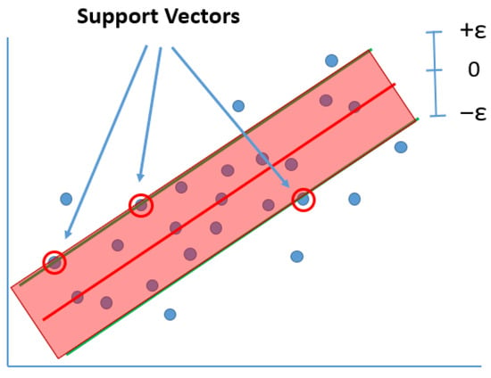
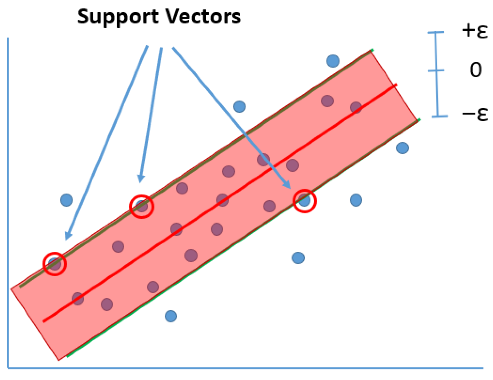
The SVR produces a convex minimization problem, avoiding local minima, which is one of its key advantages over other machine learning algorithms (Boser et al., 1992); thus, the main goal of SVR, as shown in Figure 1, is to find a function that approximates the given data points while minimizing the function’s deviation from the actual values. Moreover, deviations below a specific level, represented as ε (epsilon), are considered acceptable and are not penalized by the SVR optimization algorithm. The area defined by ε is called the error tolerance band. It describes the data so that only deviations outside this threshold ε are penalized.
The error tolerance band is critical to SVR operation. The data points that reside on or outside the boundaries of this band are called “support vectors”. To handle non-linear relationships, SVR employs kernel functions that project the original data from the initial variable space to a higher-dimensional space, called feature space, where a “linear” regression can effectively capture complex patterns. This kernel-induced transformation allows SVR to perform linear regression in the transformed space while maintaining non-linear flexibility in the original input space. In our model, we used the non-linear Radial Basis Function kernel (RBF).
The optimal model parameters are identified in a training and testing step scheme. Most of the dataset is used to train the model (identify the optimal parameters), while a smaller, separate subset is reserved to test the generalization ability of the model in unseen data (Figure 2).
Figure 2.
Support vector regression. The upper and lower error tolerance threshold are represented by the letter ε. Support vectors are the data points that lie on or outside this error tolerance band. Forecasting values greater than ε incur a penalty according to their distance from the allowed tolerance band.
2.2. Decision Trees (DTs)
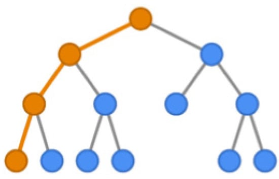
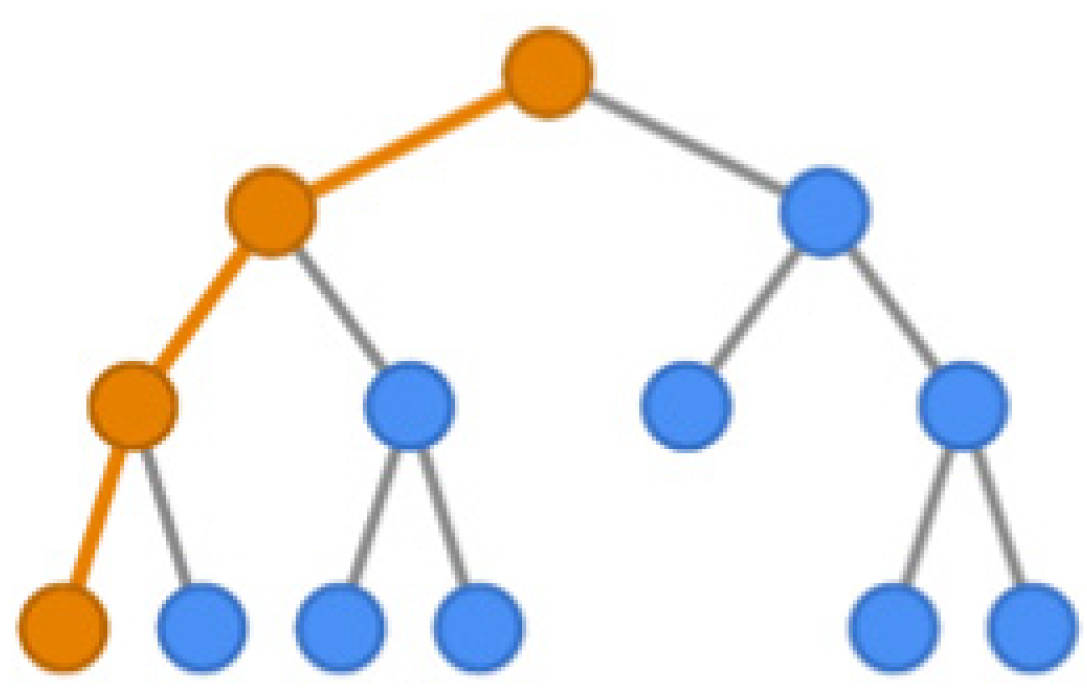
The decision tree algorithm was proposed by Breiman et al. (1984) as a forecasting modelling tool in statistics, data mining, and machine learning. While the classification trees are designed mainly for predicting categorical or discrete variables, the regression trees are tailored for predicting a continuous numerical value (typically real numbers) for the target variable. In regression prediction, a decision tree generates predictions for a new observation (new instance) by travelling over the tree’s branches based on the observation’s independent variable values. When it reaches a leaf node (end-node), the predicted value is typically computed using a statistical measure—most commonly the mean of the training instances contained within that leaf (Figure 3).
Figure 3.
Decision tree structure.
2.3. Random Forests (RFs)
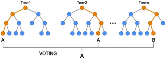
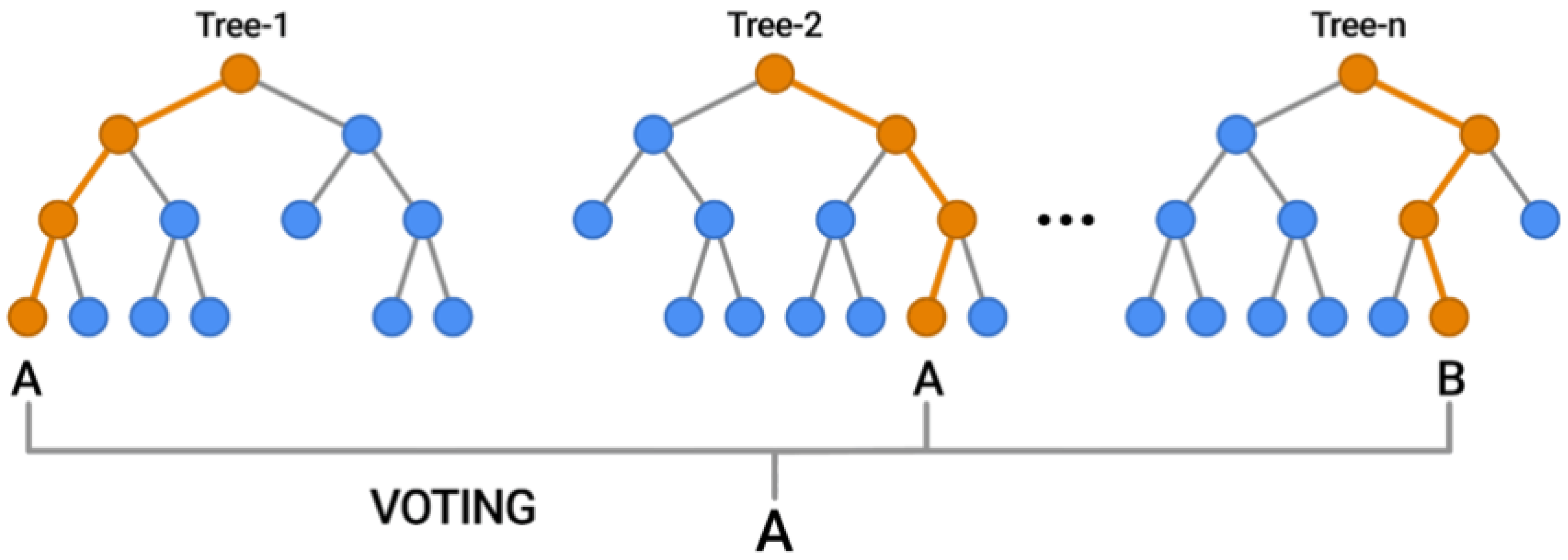
Random forests (RFs) are a supervised machine learning algorithm that is used widely in classification and regression problems. They combine the concept of decision trees with the process of bagging, i.e., bootstrapping and aggregating (Breiman, 1996). Mishina et al. (2015) recommend this method for solving the problem of overfitting by combining numerous decision trees into a single model. If our dataset has observations, for each decision tree, we create a new sample of size by randomly selecting observations from the initial dataset with replacement. The observations not selected in a tree are called “out-of-bag” observations, and they are used to test the generalization ability of the trained model; they are similar to the “out of sample” or validation set used in the SVR algorithm. Each decision tree uses a randomized subset of explanatory variables. Both the bootstrapped sets and the subset of explanatory variables used for each tree introduce randomness and thus add to the robustness of the random forest model predictions. In classification tasks, the final prediction of the random forest is usually decided by a majority vote among the trees, while in regression tasks, it is usually the average of the predictions made by each individual tree (Figure 4).
Figure 4.
Random forest capture.
2.4. Time Series Cross-Validation (TSCV) Using a Rolling (Expanding) Forecast Horizon
Before conducting any empirical analysis, we first split the whole dataset into two subsets: an 80% training sample (221 observations) and a 20% validation sample (56 observations). All model estimation, hyperparameter optimization and cross-validation (CV) is used in the training sample only to prevent the issue of overfitting.
The standard cross-validation process divides the training observations into subsamples called folds. The model is iteratively trained on n − 1 folds, using the remaining fold for testing. The performance across n test folds is then averaged using the chosen evaluation metric, the Mean Absolute Error (MAE). The optimal model is chosen as the hyperparameter configuration that produces the lowest MAE. This technique is known as “n-fold cross-validation”. However, for time series data, where observations are ordered chronologically, random shuffling is not appropriate.
In this study, we applied the time series cross-validation (TSCV) technique, also known as walk-forward validation or rolling-origin evaluation, as it is described by Armstrong et al. (1972) and Armstrong (1985), which preserves the temporal order of the data and evaluates the model on multiple sequential periods. We used a 3-fold TSCV. The training set starts with the oldest 25% of the observations, while the next 25% is used as the test fold. In the next iteration, the model is retrained on the first 50% of the observations and is tested on the subsequent 25%. This procedure is repeated across the dataset, allowing the model to be tested on multiple future periods while ensuring that future information is never used to predict past observations.
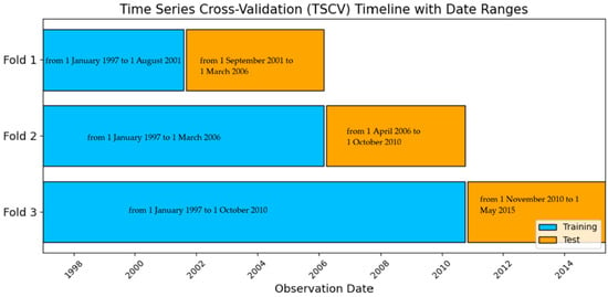
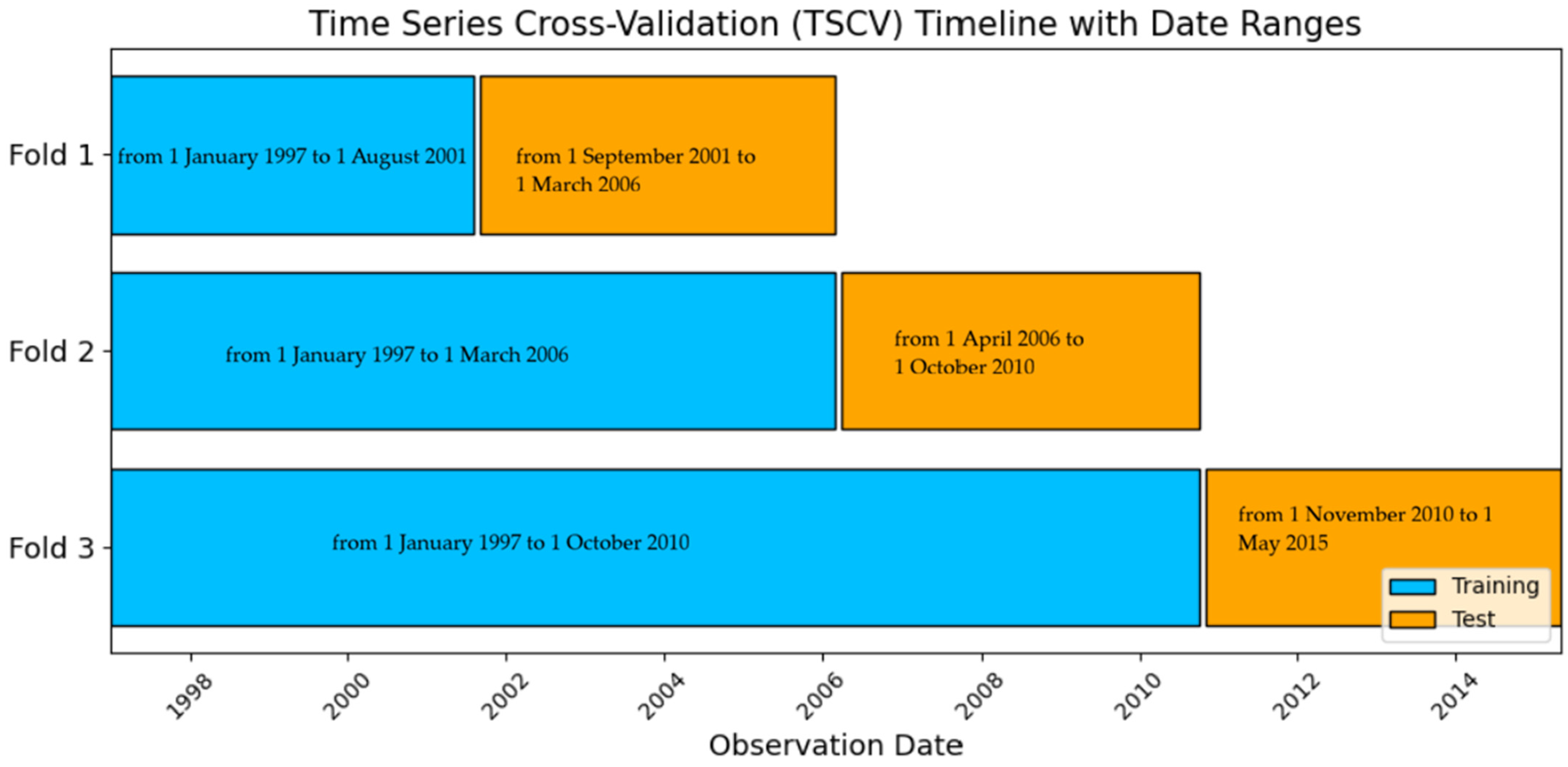
Figure 5 illustrates the start and end dates of the training and test folds of the TSCV procedure, providing a clear overview of how the data were sequentially split for model evaluation. Based on the first fold, the model is training for the first 56 observations (training: from 1 January 1997 to 1 August 2001) and tested on the next 54 observations (test: from 1 September 2001 to 1 March 2006), ensuring that the model is only using past data to predict the immediate future. Next, the training window is extended to include both folds 1 and 2, including more historical information (training: from 1 January 1997 to 1 March 2006), and the model’s performance is tested on the next 54 observations (test: from 1 April 2006 to 1 October 2010). Finally, the training window further extends to include folds 1, 2 and 3 (training: from 1 January 1997to 1 October 2010), and the performance is tested on the final 54 observations (test: from 1 November 2010 to 1 May 2015).
Figure 5.
Time series cross-validation (TSCV) for the dataset from 1997 to 2015 (80% of the total dataset). Each horizontal bar represents a fold: blue indicates the training period; orange indicates the test period.
The generalization ability of the optimized models was further assessed using the validation set, not included in any training or test set. Model performance on the training set was evaluated using various forecasting metrics: the Mean Absolute Error (MAE), the Mean Absolute Percentage Error (MAPE), the Root Mean Squared Error (RMSE), the Coefficient of Determination (R2), Symmetric Mean Absolute Percentage Error (sMAPE), and the Mean Absolute Scaled Error (MASE).
2.5. Hyperparameter Tuning
For each machine learning model, we performed hyperparameter optimization using a grid search approach combined with the time series cross-validation (TSCV) to ensure robust performance across data splits. For example, a moderately complex tree structure appears to have produced the highest predictive accuracy for the decision tree model, according to the selected hyperparameters (maximum depth of 10, no restriction on leaf nodes, and minimal sampling thresholds). The combinations show that the model gains from capturing fine-grained patterns and non-linear correlations in the data while preserving its capacity for generalization. The remaining models followed similar optimization processes.
The best hyperparameters tuned for each machine learning model are the following:
| MODEL | HYPERPARAMETERS TUNED |
| DECISION TREES | ‘max_depth’: 10, ‘max_leaf_nodes’: None, ‘min_samples_leaf’: 1, ‘min_samples_split’: 2 |
| RANDOM FOREST | ‘model max_depth’: 10, ‘model_min_samples_leaf’: 1, ‘model_min_samples_split’: 5, ‘model_n_estimators’: 100 |
| XGBOOST | ‘colsample_bytree’: 1.0, ‘gamma’: 0, ‘learning_rate’: 0.1, ‘max_depth’: 3, ‘n_estimators’: 100, ‘subsample’: 0.7 |
| SVR_RBF | model__C’: 1, ‘model__epsilon’: 0.001, ‘model_gamma’: ‘scale |
| SVR_LINEAR | ‘svr__C’: 0.1, ‘svr__epsilon’: 0.1 |
2.6. Feature Scaling
Feature scaling is a vital step in preparing the data for machine learning algorithms. Many machine learning algorithms are sensitive to characteristics on different scales because they calculate the distances between data points. Similar-scale features can enhance these algorithms’ performance. In this paper, we scale the independent variables via standardization. Standardization transforms the independent variables so that they follow a distribution with zero mean and unit variance:
where Z is the standardized value, x is the original variable value, μ is the mean of the variable, and σ is its standard deviation.
2.7. SARIMA
Seasonal Autoregressive Integrated Moving Average (SARIMA) is a variation of the standard ARIMA model that is used to forecast time series data exhibiting seasonal patterns. These models are designed to capture both non-seasonal and seasonal components, making them suitable for datasets with periodic fluctuations. We account for possible non-stationarity by using the following specification:
where p, d, and q describe the orders of the non-seasonal AR, the differencing, and the MA. Similarly, P, D, and Q describe the orders of the seasonal relevant parameters. Finally, s is the length of the seasonal cycle (e.g., 12 for monthly data with annual seasonality). The trend and seasonal components’ non-stationarity are appropriately addressed through the differencing orders d and D.
SARIMA(p, d, q) (P, D, Q, s)
2.8. Forecast Evaluation Metrics
The accuracy of our models is evaluated using several forecasting metrics: the Mean Absolute Percentage Error (MAPE), the Root Mean Squared Error (RMSE), the Mean Absolute Error (MAE), the Coefficient of Determination (R2), the Symmetric Mean Absolute Percentage Error (sMAPE), and the Mean Absolute Scaled Error (MASE).
Τhe Mean Absolute Error (MAE) and Root Mean Squared Error (RMSE) are employed to quantify the average magnitude of the prediction errors in the same units as the target variable. MAE measures the average absolute deviation between observed and predicted values, treating all errors (positive or negative) equally, while RSME is the square root of the mean square error, which makes the scale of errors equal to the scale of targets.
They are calculated in the following standard way:
where is the actual value, is the predicted value i, and n is the total number.
Percentage-based error measures, namely the Mean Absolute Percentage Error (MAPE) and Symmetric Mean Absolute Percentage Error (sMAPE), are used to assess forecasting accuracy in relative terms. MAPE is a measure for regression models which provides the error as a percentage, allowing for a more accurate estimate of error, and it offers a scale-independent metric of the error. This is especially beneficial in situations where it is critical to understand the extent of the error in relation to the real value. However, in some cases MAPE could become undefined or unstable when actual values get close to zero. To address this limitation, sMAPE is also considered. By symmetrically normalizing the absolute error using both actual and predicted values, sMAPE reduces sensitivity to outliers and avoids division by zero issues, making it more reliable for time series data with low (close to zero) or unstable observations.
MAPE and sMAPE are calculated in the following standard way:
where denotes the actual observed value of the target variable at time t, represents the corresponding forecasted value generated by the model, and n is the number of observations.
The Mean Absolute Scaled Error (MASE) is employed as a scale-independent performance metric that benchmarks the forecasting model against a naïve in-sample forecasting method. MASE is computed as the ratio between the model’s MAE and the MAE obtained from a naïve one-step-ahead forecast applied to the training data.
Finally, the R2 calculates what percentage of the variance in the target (dependent) variable is explained by the forecasting model. It is computed as follows:
where:
(Residual Sum of Squares) is the unexplained variance. It is the sum of the squares of the differences between the actual values and the predicted values ().
(Total Sum of Squares) is the total variation in the data. It is the sum of the squares of the differences between each actual value and the mean of the actual values (.
For all error-based metrics (MAPE, RMSE, MAE, sMAPE, and MASE), smaller values indicate better forecast accuracy, with zero representing a perfect prediction. The use of MASE provides a scale-independent measure that can be applied across different seasonal and trend patterns (Lima et al., 2024). In contrast, when R2 values are close to 1, this indicate that the model explains a higher proportion of the variance in the observed data (Nakagawa et al., 2013).
3. The Data
We have compiled a dataset with monthly frequency spanning from February 1989 to February 2020, containing a total of 277 observations and 58 variables We did not collect any data after February 2020 due to the COVID-19 pandemic and the relevant government policies that effectively prohibited transportation and tourism at an international and national level. The initial dataset was selected to cover multiple dimensions potentially influencing UK tourism demand. In addition to the Office for National Statistics (ONS) data, we included additional variables not routinely covered by official statistics, aiming to enhance the analysis and provide a more comprehensive view of factors influencing inbound tourism arrivals. Thus, our variable selection was based on the following factors: (a) the relevant literature on tourism demand, (b) availability of the data, and (c) an exploratory study to include a wide range of possible other determinants of tourism demand and their interrelations that were not directly used, explored or empirically tested previously in the literature.
Our rich dataset includes variables from five different groups:
- (a)
- Macroeconomic indicators: Macroeconomic indicators reflect the overall economic health and stability of the country, which can have a significant impact on tourism demand.
- (b)
- Leisure and travel metrics: These provide a thorough overview of the country’s tourism activity by describing the movements of visitors, spending habits and their travel preferences.
- (c)
- Consumer goods and services indicators: Since travel is typically viewed as a luxury or non-essential activity, these variables capture trends in discretionary spending, which is closely linked to tourism spending. Increased spending on jewellery, watches, durable goods, or personal hygiene products is often an indicator of better economic conditions and rising consumer confidence, all of which are associated with a greater desire to travel (Tkalec & Vizek, 2016). As a result, these measures act as proxies for more general consumption patterns that change in line with households’ propensity to spend on travel.
- (d)
- Climate and weather conditions: The variables related to climate and weather conditions reflect the country’s attractiveness as a tourist destination and its ability to cater to the preferences and needs of travellers (Falk & Lin, 2018).
- (e)
- Exchange rates and financial markets: Exchange rates and their volatility affect tourism demand, as tourists prefer stable exchange rates when planning trips (Rookayyah et al., 2024; Webber, 2001). Stock market indices, such as the NASDAQ-100 and the EURO STOXX 50, serve as indicators of market sentiment.
To avoid redundancy and multicollinearity, we examined the correlations in our dataset and removed highly correlated variables, keeping only one representative variable from each correlated cluster/category. This refinement resulted in a clean dataset that retains most of the information content of the original dataset, while improving the robustness and interpretability of the models. The variables removed during this refinement step include CPI transport; minimum temperature; S&P 500; passenger transport by railway; passenger transport by air; passenger transport by road; passenger transport by sea and inland waterway; package holidays; restaurants and hotels; restaurants—cafés and the like; accommodation services; TargeT + 11; and CAC 40 (^FCHI).
In Table 1, we present the full list of the variables used in our dataset.
Table 1.
Description of explanatory variables.
4. Empirical Results
4.1. Machine Learning Algorithms
The goal of our study is to create a model that accurately forecasts overseas tourist arrivals in the U.K. To achieve this, we trained the optimal model for each algorithm using 80% of the full sample as the training set, while keeping the remaining 20% as the validation sample, which does not take part in the training process. The optimal model for each algorithm was selected using the MAPE metric in the training set. To avoid over-fitting, we used a three-fold rolling time series cross-validation scheme. To assess the generalization ability of each model, we present the forecasting metrics of both the training and the validation sets.
In the case of the random forests, as the validation set, we use the relevant out-of-bag (OOB) subset instead of a predefined validation (out-of-sample) subset. The OOB subset includes all observations that were not selected during the bootstrapping step inherent in the random forest algorithm. Table 2 presents the forecasting metrics for all trained algorithms, both in the training (in-sample) and the validation (out-of-sample) subsets.
Table 2.
Performance comparison of forecasting methodologies for machine learning models.
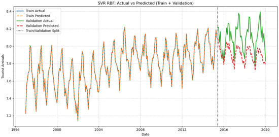
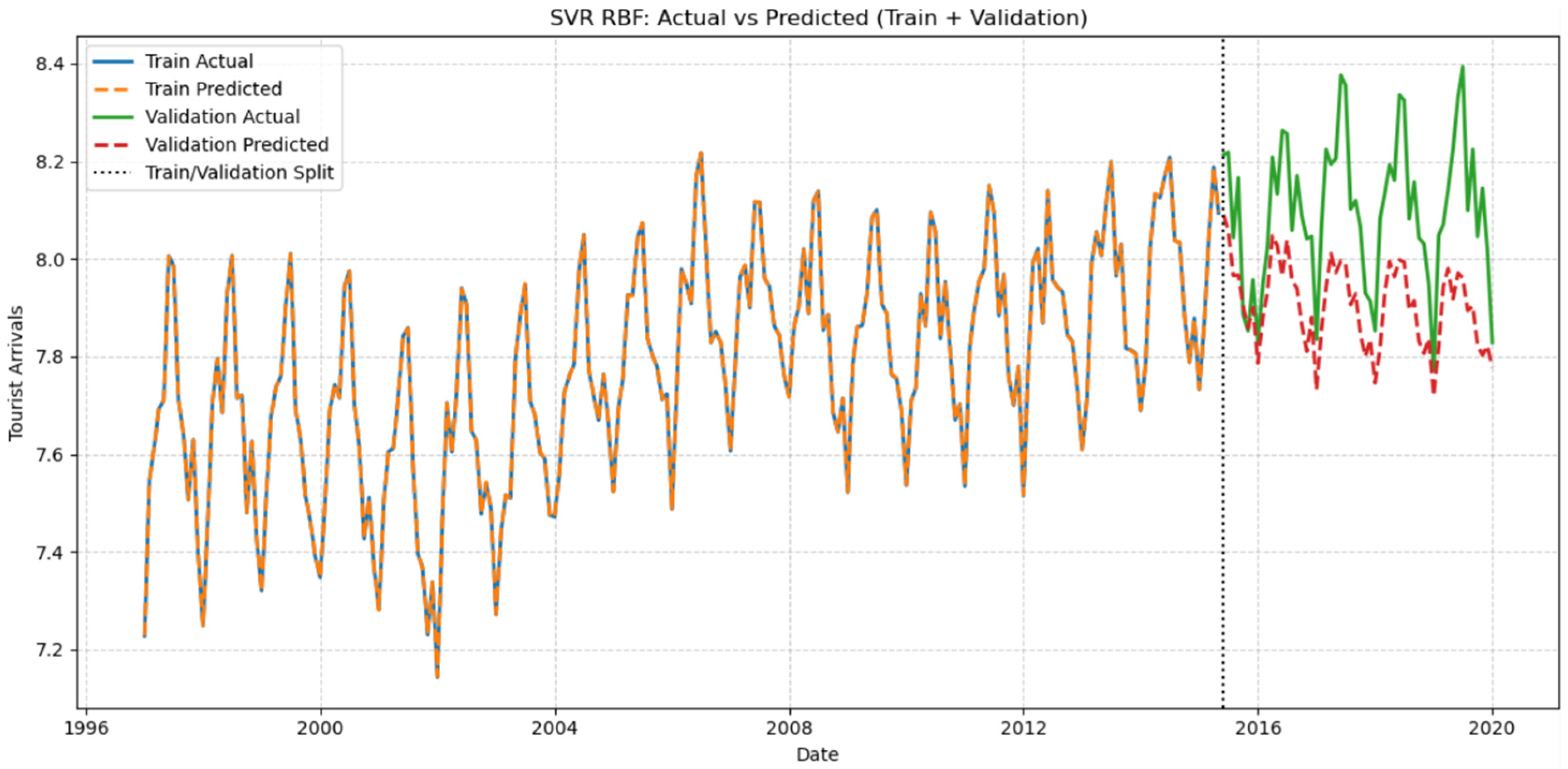
The results on the training (in-sample) highlight that all the machine learning models substantially outperform the traditional SARIMA model on the training data, as demonstrated by the matrix values significantly lower than one. A low MAPE but negative R squared value is a common pattern in models fitted to difference series, where the reduction in variance leads to smaller percentage error, while R2 may become negative. The best model is the SVR-RBF which achieves an MAPE of 0.014%, an RMSE of 0.001, an MAE of 0.192, R2 of 1.00, an sMAPE of 0.014%, and an MASE of 0.009, indicating a very strong fit in the training data.
These results imply that machine learning techniques can greatly increase the precision of tourism demand forecasting in the UK from an economic and tourism management perspective. For tourism stakeholders, accurate demand estimation offers crucial information that facilitates decision making, allowing them to create and successfully execute policies. Moreover, hospitality providers, destination management organizations and policymakers can effectively plan personnel levels, infrastructure needs, and resource allocation. More accurate forecasting can facilitate better workforce management, hotel capacity planning and transportation service scheduling for periods of high tourism. Furthermore, accurate tourism demand predictions play a crucial role in developing targeted marketing campaigns and strategies by enabling businesses and policymakers to anticipate future visitor trends (Khatibi et al., 2022).
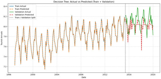
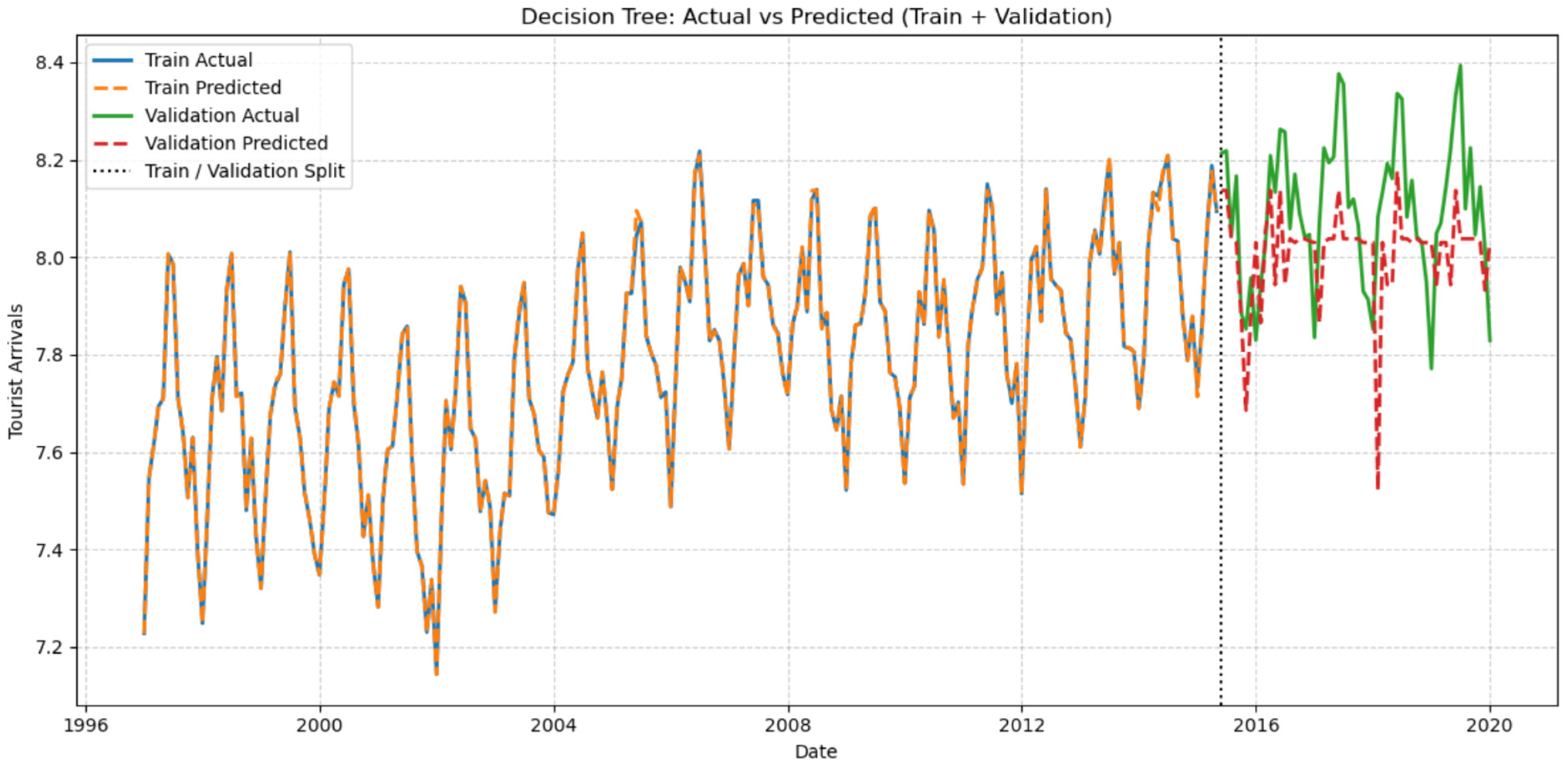
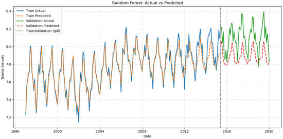
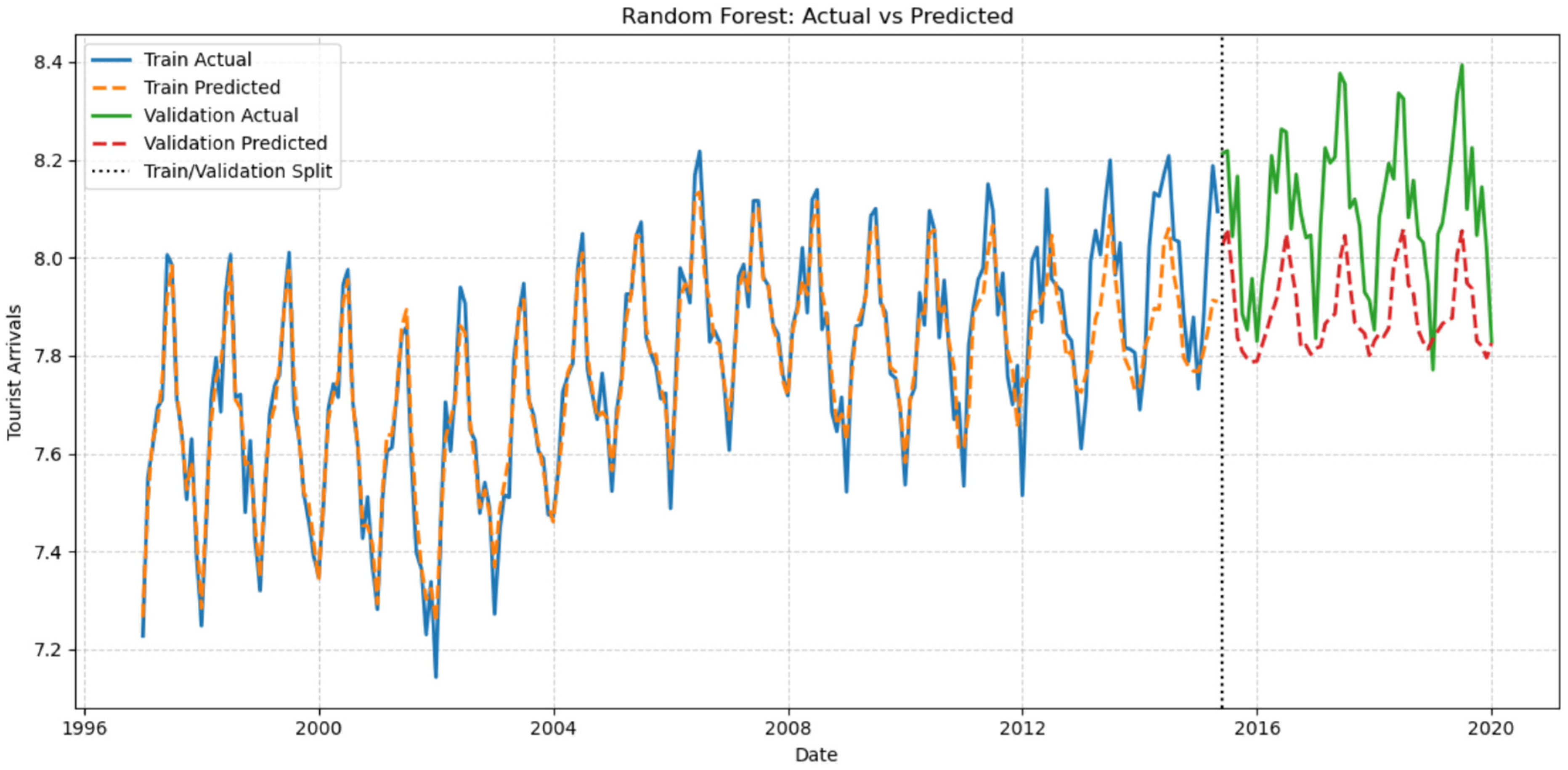
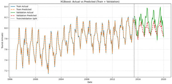
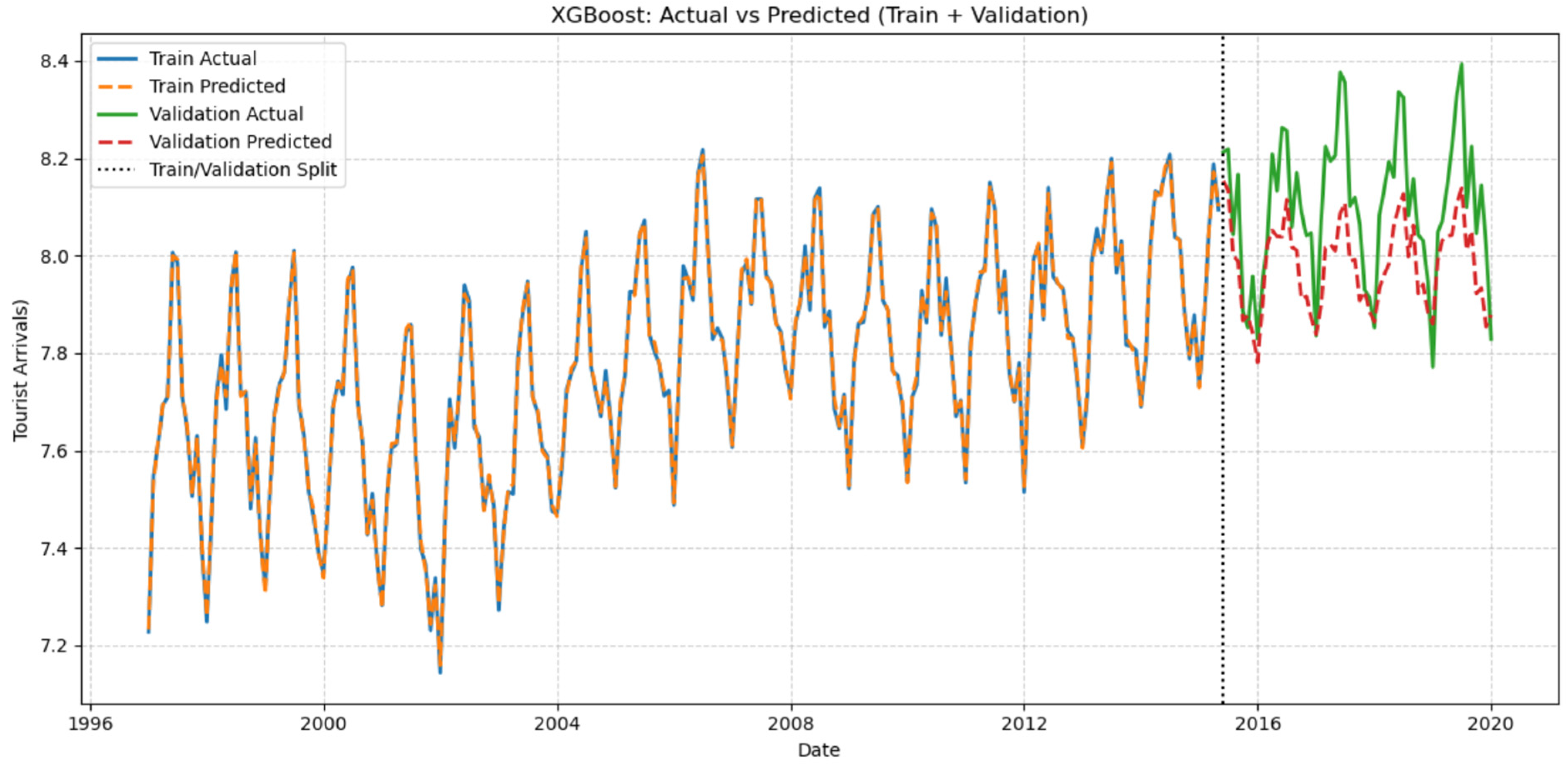
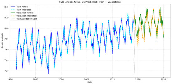
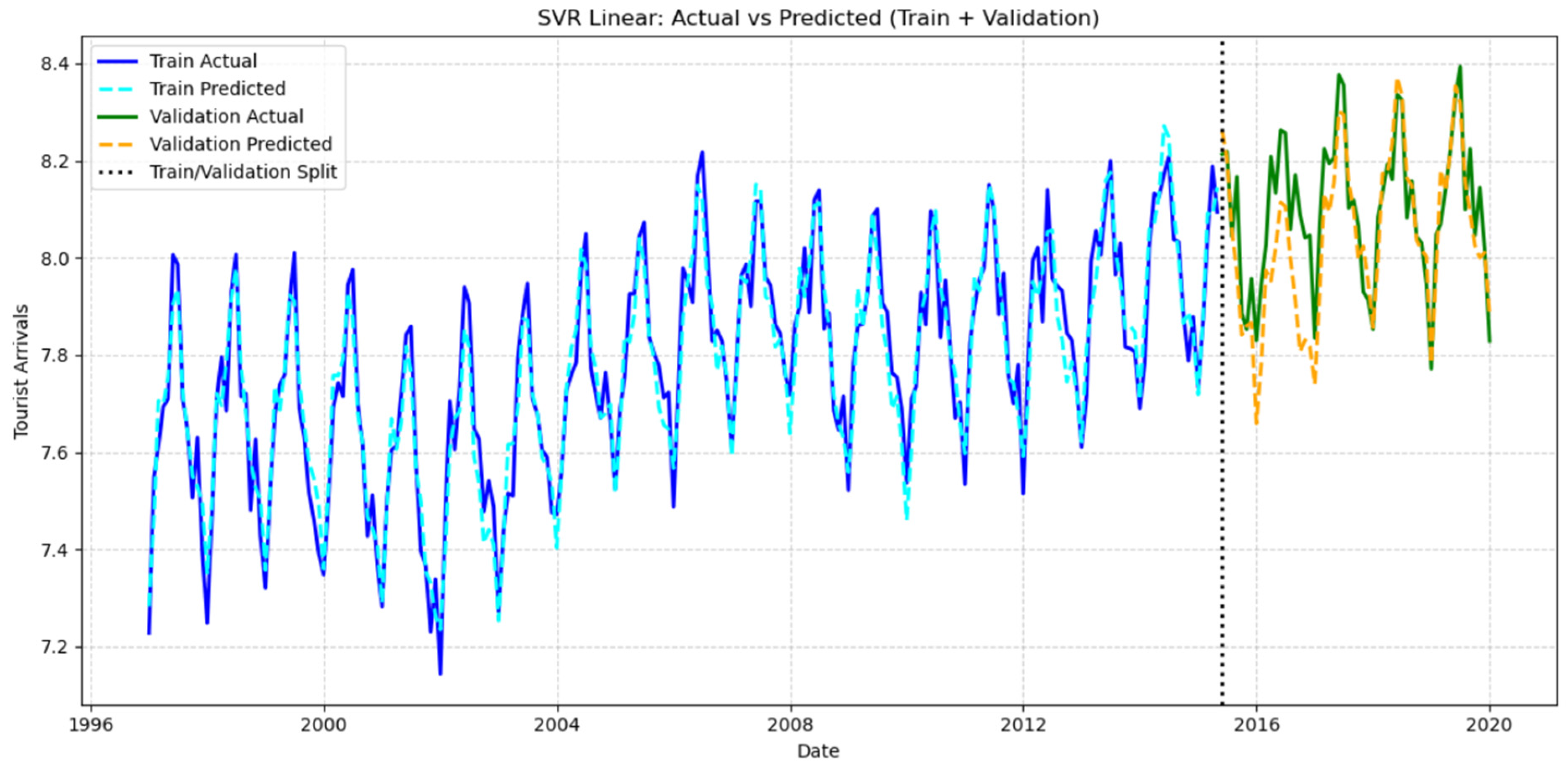
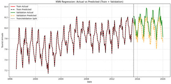
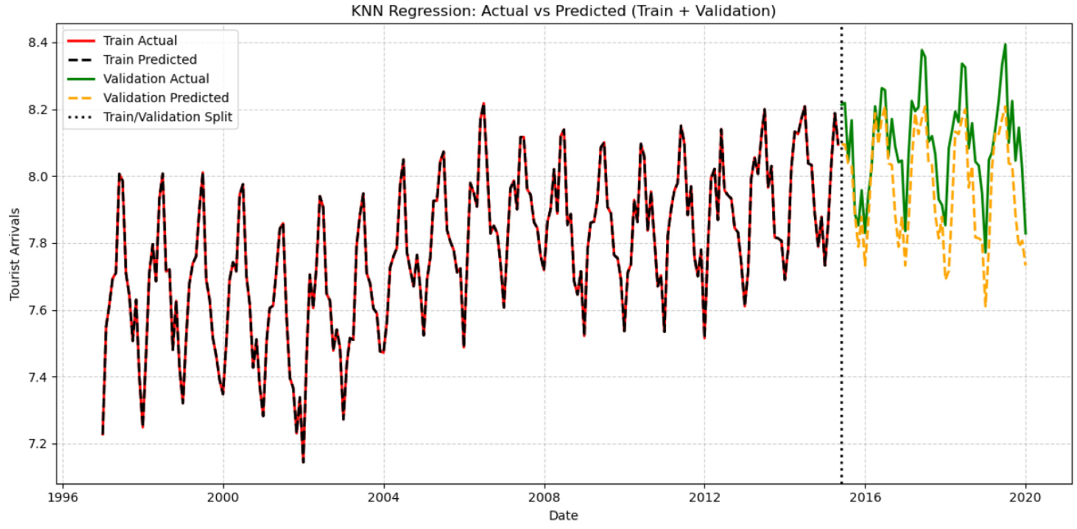
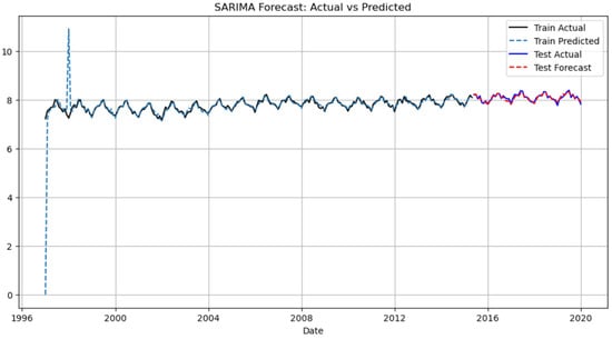
A visual depiction the performance of our models can be found in Figure 6, Figure 7, Figure 8, Figure 9, Figure 10, Figure 11 and Figure 12. These figures include both the forecasted values and the actual inbound tourism demand. The first part, on the left of the vertical line, refers to the training (in-sample) set, and the last part to the validation (out-of-sample) set.
Figure 6.
Actual vs. predicted tourist arrival values—decision tree model (applying grid search) on both the training and validation samples.
Figure 7.
Actual vs. predicted tourist arrival values—random forest model (applying grid search) on both the training and validation samples.
Figure 8.
Actual vs. predicted tourist arrival values—XGBoost model (applying grid search) on both the training and validation samples.
Figure 9.
Actual vs. predicted tourist arrival values—SVR-RBF model (applying grid search) on both the training and validation samples.
Figure 10.
Actual vs. predicted tourist arrival values—SVR linear kernel (applying grid search) on both the training and validation samples.
Figure 11.
Actual vs. predicted tourist arrival values—K-neighbours regression model (applying grid search) on both the training and validation samples.
Figure 12.
Actual vs. predicted tourist arrival values—SARIMA model on the training sample.
4.2. SARIMA Results
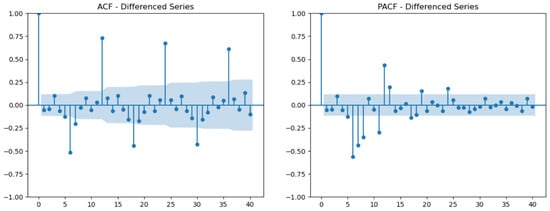
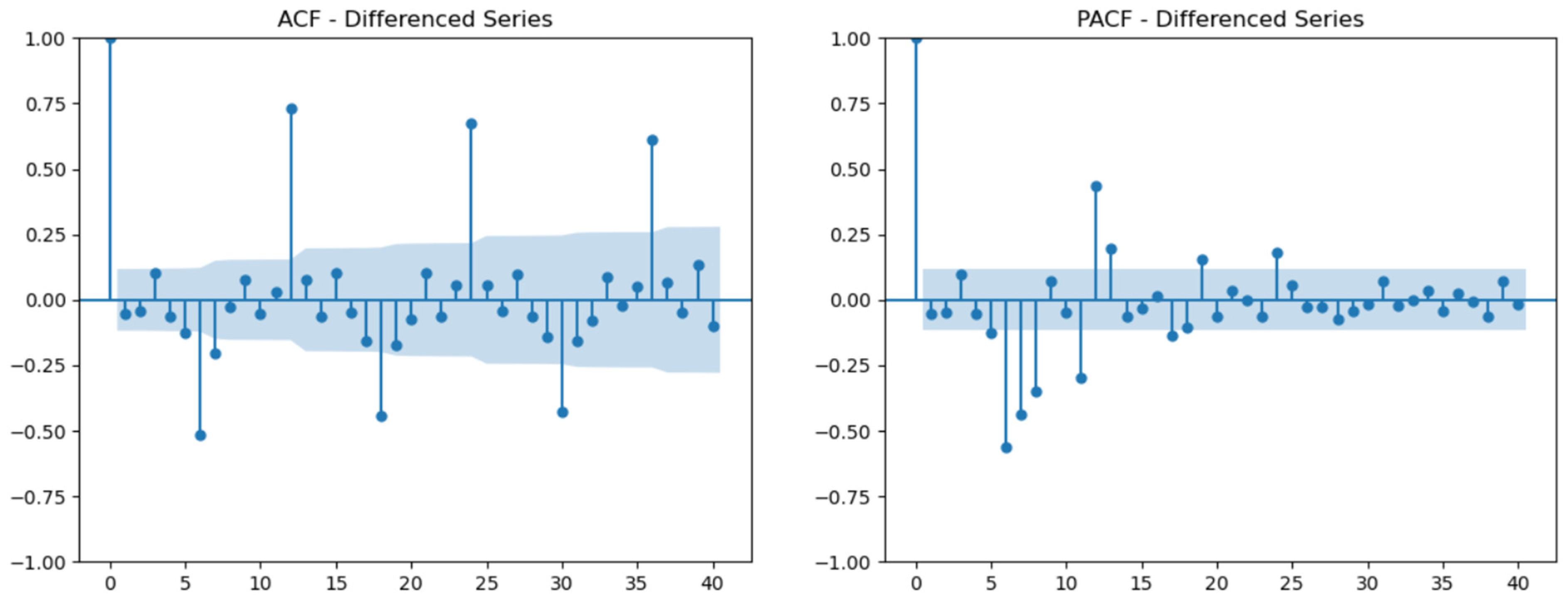
Figure 13 illustrates the autocorrelation (ACF) and partial autocorrelation (PACF) of the differenced series following first-order (d = 1) and seasonal (D = 0) differencing with a 12-month period (s = 12). The ACF illustrates both short-run and seasonal moving-average behaviour, characterized by a notable negative spike at lag 1 and a strong positive seasonal spike at lag 12. The PACF also shows a significant spike at lag 1 and a seasonal influence at lag 12, consistent with autoregressive structure in both non-seasonal and seasonal components. Most of the autocorrelation values fall within the 95% confidence bounds, indicating that the series has reached stationarity. These patterns are characteristic of seasonal time series processes and support the inclusion of a seasonal moving-average (Q = 1) and seasonal autoregressive (P = 1) component in the SARIMA specification. Based on the ACF/PACF diagnosis and the lowest Akaike Information Criterion (AIC) (—525.56), the SARIMA (0, 1, 1) (1, 0, 1, 12) model was selected as the optimal specification for capturing the seasonal dynamics of the series.
Figure 13.
ADF and PACF differenced series.
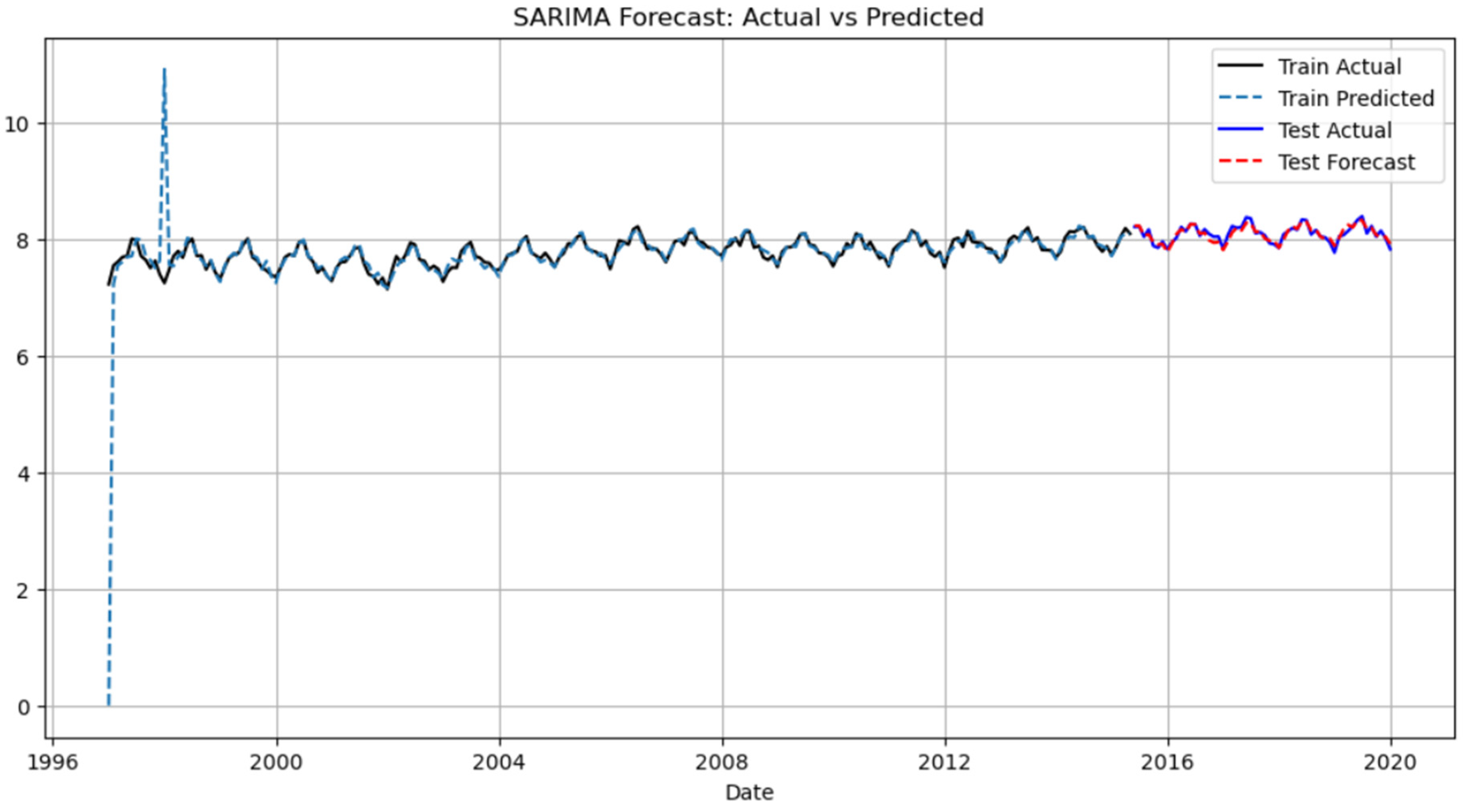
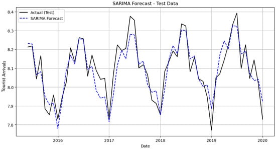
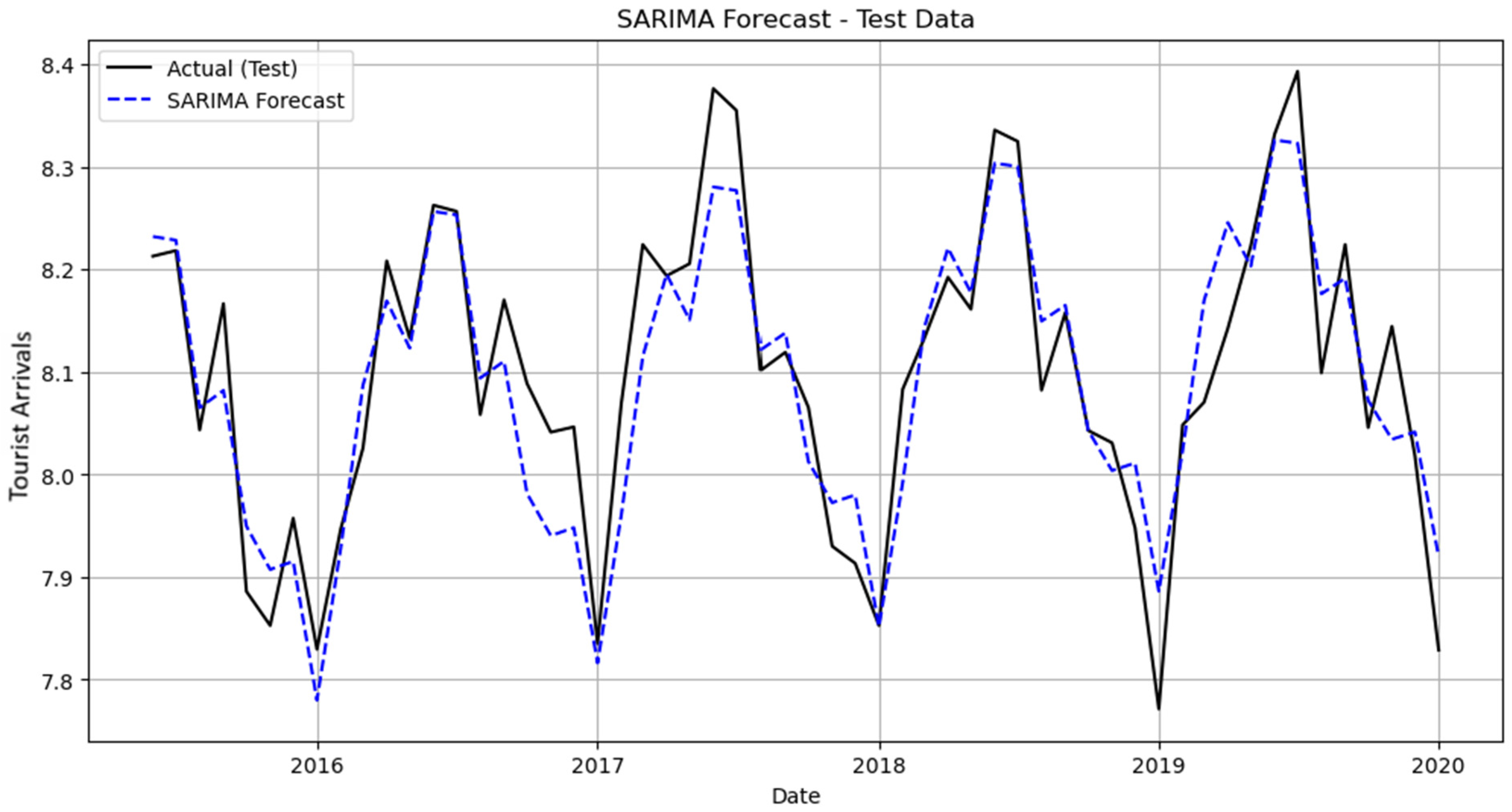
Figure 14 illustrates the out-of-sample forecasts for the test period. In the out-of-sample period, the model maintains strong predictive alignment with actual values, successfully reproducing seasonal peaks and troughs over multiple years. The strong generalization of the model beyond the testing data is confirmed by the robust validation metrics (MAPE, RMSE, MAE, R2, sMAPE, and MASE), which further support the visual evidence.
Figure 14.
Actual vs. predicted tourist arrival values—SARIMA model on the test sample (out-of-sample validation).
4.3. Feature Importance
Next, we apply the feature importance technique, which provides insights into the contribution of each of the features to the forecasting ability of our model, offering a deeper understanding of the drivers of the UK inbound tourism demand. The top 15 variables, based on their feature importance coefficients, are presented in Table 3 (The full list with all independent variables can be found in Appendix A). The findings show that several macroeconomic, environmental, and seasonal factors are important in explaining UK inbound tourism demand. It is important to note that the weather indicators used in this study refer to the observed values of the current month, rather than forecasts for the following month. This distinction is important since weather forecasts for longer time horizons are usually highly imprecise, making them unrealizable predictors of tourism demand.
Table 3.
Top 15 variables ranked by feature importance. The full list with all independent variables can be found in Appendix A.
The most significant variable is “JANS04” (FI = 0.1368) providing evidence that seasonal effects of winter, especially January, have a major impact on tourism demand. Studies have shown that seasonality has a strong impact on tourist arrivals, with a significant amount of the volatility in visitors attributed to seasonal variation. For example, Hossen et al. (2021) found that both winter and summer play a major role in the seasonality of tourism demand.
The findings indicate that current conditions significantly influence travel planning decisions for the subsequent month. Table 3 shows that the variables “Sun” (FI = 0.0996) and “Tmax” (FI = 0.0612) indicate that favourable weather conditions, such as more sunshine and higher temperatures have a beneficial impact on tourism demand, appearing as the second and fourth most important variables, respectively. These results are consistent with the existing literature, which indicates that weather-related variables—temperature, sunshine, rainfall, and climate conditions—in origin countries are among the important predictors influencing tourist arrivals, affecting both the timing and volume of tourism demand (Becken, 2013; Baig et al., 2021; Gricar et al., 2021).
Additionally, seasonality effects remain important, consistent with the previous tourism demand literature. Lagged values of the dependent variable, TargeT-5, TargeT-4, and TargeT-6, contribute significantly to forecasting performance, ranked third, fifth, and sixth, respectively. This implies that visitor arrivals show temporal persistence, which means that demand for travel today is greatly influenced by historical tourism levels. Furthermore, macroeconomic variables, such as UK Inflation and USA Inflation (lagged), appear in the top-ranked variables, as 9th, 10th, 11th, and 13th in variable importance. Inflation has a detrimental effect on tourism arrivals as higher inflation can weaken traveller’s purchasing power and raise travel expenses, which could result in fewer visitors arriving, especially among low-budget tourists or price-sensitive tourists and in places where there is political or economic uncertainty (Pernas et al., 2025; Raifu & Afolabi, 2026).
5. Conclusions
Given that tourism is a significant component of the UK GDP, accuracy in forecasting monthly visitor arrivals is important for economic resource planning, especially at the macroeconomic level. Overestimated or underestimated forecast values have an impact on the optimal distribution of relevant adequate tourism resources in terms of capital and labour. Tourism demand has sparked a growing interest in employing new and advanced forecasting approaches, such as ML techniques. In this paper, we evaluated the performance of various machine learning algorithms and compared them to the more traditional econometric SARIMA model. The data used are in monthly frequency from February 1989 to February 2020, for a total of 277 observations. The machine learning algorithms that we employed were decision trees, random forests, support vector regression using both the RBF and the linear kernel, and XGBoost. Moreover, we also employed a more traditional econometric model, the SARIMA. We include a wide collection of explanatory variables (55) that are based on the relevant tourism demand literature. The results show that from all the models used, the support vector regression coupled with the RBF kernel model is the best one as it provides the minimum MAPE metric at 0.014% when evaluated within the time series cross-validation (TSCV) procedure. The second best was the XGBoost model, with an MAPE of 0.101%.
To shed more light in the so-called “black-box” limitation of machine learning models, we also employed the feature importance ranking technique to provide a more transparent and comprehensive framework for understanding how each independent variable contributes to the model’s predictions. The results show that seasonality, trends, weather conditions and macroeconomic factors play a significant role in tourism demand. This is evidenced by relevant variables appearing in the top 15 ranking. This feature importance ranking suggests that seasonality plays an important role as five out of the top 15 independent variables are monthly seasonal dummies. Tourist demand demonstrated significant seasonal regularity, consistent with established findings in the tourism forecasting literature. Moreover, historical trends in tourist arrivals, are ranked in third, fifth and sixth place as the most important indicators of future tourist arrivals. This result suggests a medium-term memory of tourism demand that is possibly the result of current trends, marketing strategies and other such factors. Furthermore, weather conditions such as sunshine hours and maximum temperature appear as the second and fourth most important variables, respectively, suggesting that tourist arrivals in the UK are significantly driven by weather conditions. Finally, the effects of both the UK and the US lagged inflation rates seem to be significant predictors of tourism demand, as they rank in 9th, 10th, 11th and 13th place in variable feature importance.
These results provide significant information needed for short-to-medium-term economic planning and facilitation of tourism demand in the UK for macroeconomic stakeholders, e.g., the central and local governments. Relevant policymakers and other tourism stakeholders can more accurately predict changes in visitor demand, which have a direct impact on tourism-related income, employment, and infrastructure utilization, facilitating more effective workforce planning, transit services, and accommodation capacity allocation during peak and off-peak seasons. Given the significant contribution of tourism to the UK economy, the improved forecasting performance of the machine learning models provides valuable support for data-driven decision-making and sustainable tourism development.
Furthermore, the study contributes to the literature by employing a long-term perspective, studying UK tourism demand over three decades and offering insights into the evolving relationship between economic conditions and tourism. This study also uncovers individual links between economic indicators and tourism flows, illustrating the marginal effects of the most influential variables.
Despite these contributions, this study has some limitations. Because the study is based on monthly data, it may overlook extremely short-term fluctuations in tourism demand, i.e., weekly or daily, and also longer-term frequences, i.e., quarterly or annual tourism arrivals. Also, another avenue to pursue future research in this area would be to apply the proposed methodology to more disaggregated tourism data, such as leisure and business travel, or visitors from different geographic origins, including demographic data to better capture differences in travel behaviour and improve forecasting accuracy at the microeconomic level, aiding tourism operators, hotels and other related firms.
Overall, this study provides useful information for policymakers by highlighting the effectiveness of machine learning techniques in predicting tourist arrivals in the UK on a monthly basis. Since policymakers rely on accurate predictions of tourist arrivals, the findings of this study have important implications for strategic decision-making in the tourism industry, as it provides insights into future trends in developing appropriate tourism support strategies.
Author Contributions
Conceptualization, A.D.; Methodology, A.D., T.P. and P.G.; Validation, A.D., T.P. and P.G.; Formal analysis, A.D., T.P. and P.G.; Investigation, T.P. and P.G.; Data curation, A.D.; Writing—original draft, A.D.; Writing—review & editing, A.D., T.P. and P.G.; Visualization, A.D. and P.G.; Supervision, T.P. and P.G.; Project administration, T.P. and P.G. All authors have read and agreed to the published version of the manuscript.
Funding
This research received no external funding. The APC was funded by the University of Lancashire Open Access Fund.
Data Availability Statement
The data presented in this study are available on request from the corresponding author.
Conflicts of Interest
The authors declare no conflict of interest.
Appendix A
Table A1.
All variables ranked by feature importance.
References
- Armstrong, J. S. (1985). Long-range forecasting: From crystal ball to computer (2nd ed.). John Wiley & Sons. [Google Scholar]
- Armstrong, J. S., & Grohman, M. C. (1972). A comparative study of methods for long-range market forecasting. Management Science, 19(2), 211–221. [Google Scholar] [CrossRef] [Scilit]
- Baig, S., Khan, A. A., & Khan, A. A. (2021). A time series analysis of causality between tourist arrivals and climatic effects for nature-based tourism destinations: Evidence from Gilgit-Baltistan, Pakistan. Environment, Development and Sustainability, 23(4), 5035–5057. [Google Scholar] [CrossRef] [Scilit]
- Becken, S. (2013). Measuring the effect of weather on tourism: A destination- and activity-based analysis. Journal of Travel Research, 52(2), 156–167. [Google Scholar] [CrossRef] [Scilit]
- Boser, B. E., Guyon, I. M., & Vapnik, V. N. (1992). A training algorithm for optimal margin classifiers. ACM. [Google Scholar]
- Breiman, L. (1996). Bagging predictors. Machine Learning, 24, 123–140. [Google Scholar] [CrossRef] [Scilit]
- Breiman, L., Friedman, J., Stone, C. J., & Olshen, R. A. (1984). Classification and regression trees (1st ed.). Taylor & Francis. [Google Scholar]
- Chen, K.-Y., & Wang, C.-H. (2007). Support vector regression with genetic algorithms in forecasting tourism demand. Tourism Management, 28(1), 215–226. [Google Scholar] [CrossRef] [Scilit]
- Chen, R., Liang, C.-Y., Hong, W.-C., & Gu, D.-X. (2015). Forecasting holiday daily tourist flow based on seasonal support vector regression with adaptive genetic algorithm. Applied Soft Computing, 26, 435–443. [Google Scholar] [CrossRef] [Scilit]
- Claveria, O., & Torra, S. (2014). Forecasting tourism demand to Catalonia: Neural networks vs. time series models. Economic Modelling, 36, 220–228. [Google Scholar] [CrossRef] [Scilit]
- Cortes, C., & Vapnik, V. (1995). Support-vector networks. Machine Learning, 20(3), 273–297. [Google Scholar] [CrossRef] [Scilit]
- Dimitriadou, A., Gogas, P., & Papadimitriou, T. (2024). Tourism and uncertainty: A machine learning approach. Current Issues in Tourism, 28(14), 2278–2298. [Google Scholar] [CrossRef] [Scilit]
- Falk, M., & Lin, X. (2018). Sensitivity of winter tourism to temperature increases over the last decades. Economic Modelling, 71, 174–183. [Google Scholar] [CrossRef] [Scilit]
- Gricar, S., Baldigara, T., & Šugar, V. (2021). Sustainable determinants that affect tourist arrival forecasting. Sustainability, 13(17), 9659. [Google Scholar] [CrossRef] [Scilit]
- Haryanto, T. (2020). Editorial: COVID-19 pandemic and international tourism demand. JDE (Journal of Developing Economies), 5(1), 1–4. [Google Scholar] [CrossRef] [Scilit]
- Havranek, T., & Zeynalov, A. (2021). Forecasting tourist arrivals: Google trends meets mixed-frequency data. Tourism Economics: The Business and Finance of Tourism and Recreation, 27(1), 129–148. [Google Scholar] [CrossRef] [Scilit]
- Hossen, S. M., Ismail, M. T., Tabash, M. I., & Anagreh, S. (2021). The impact of seasonality on tourist’s arrival in Bangladesh by using Sancova model. Geo Journal of Tourism and Geosites, 38(4), 1118–1124. [Google Scholar] [CrossRef] [Scilit]
- Khatibi, A., Couto da Silva, A. P., Almeida, J. M., & Gonçalves, M. A. (2022). A quantitative analysis of the impact of explicit incorporation of recency, seasonality and model specialization into fine-grained tourism demand prediction models. PLoS ONE, 17, e0278112. [Google Scholar] [CrossRef] [Scilit]
- Li, X., & Law, R. (2020). Forecasting tourism demand with decomposed search cycles. Journal of Travel Research, 59(1), 52–68. [Google Scholar] [CrossRef] [Scilit]
- Lima, S., Gonçalves, A. M., & Costa, M. (2024). Predictive accuracy of time series models applied to economic data: The European countries retail trade. Journal of Applied Statistics, 51(9), 1818–1841. [Google Scholar] [CrossRef] [Scilit] [PubMed]
- Liu, X., Liu, A., Chen, J. L., Li, G., & Song, H. (2026). Tourism demand forecasting in normal and crisis times: Combining bootstrap-aggregating and Bayesian approaches. Journal of Hospitality & Tourism Research, 50(3), 323–340. [Google Scholar] [CrossRef] [Scilit]
- Martin, C. A., & Witt, S. F. (1989). Forecasting tourism demand: A comparison of the accuracy of several quantitative methods. International Journal of Forecasting, 5(1), 7–19. [Google Scholar] [CrossRef] [Scilit]
- Mishina, Y., Ryuei, M., Yuji, Y., Takayoshi, Y., & Hironobu, F. (2015). Boosted random forest. IEICE Transactions on Information and Systems, 98(9), 1630–1636. [Google Scholar] [CrossRef] [Scilit]
- Nakagawa, S., Schielzeth, H., & O’Hara, R. B. (2013). A general and simple method for obtaining R2 from generalized linear mixed-effects models. Methods in Ecology and Evolution, 4, 133–142. [Google Scholar] [CrossRef] [Scilit]
- Office for National Statistics (ONS). (2020). UK tourism satellite account 2018. ONS. Available online: https://cy.ons.gov.uk/releases/uktourismsatelliteaccount2018 (accessed on 7 April 2026).
- Pernas, J. B., Oya, J. V., & González, J. A. P. (2025). What if prices change? Analysis of international tourist market segments’ composition in the face of inflation fluctuations. Cuadernos de Turismo, (55), 91–115. [Google Scholar] [CrossRef] [Scilit]
- Raifu, I. A., & Afolabi, J. A. (2026). Does rising inflation affect the tourism industry? Evidence from Nigeria. Journal of Policy Research in Tourism, Leisure and Events, 18(1), 167–183. [Google Scholar] [CrossRef] [Scilit]
- Rookayyah, I., Seetanah, B., Nunkoo, R., & Jaffur, Z. K. (2024). The impact of exchange rate and exchange rate volatility on tourism demand using disaggregated data. The International Journal of Tourism Research, 26(2), e2640. [Google Scholar] [CrossRef] [Scilit]
- Song, H. (2003). Forecasting tourism demand: Methods and strategies by Douglas C. Frechtling. Butterworth Heinemann, Oxford, 2001. no. of pages: 274. price L49.99. ISBN 0-7506-5170-9. The International Journal of Tourism Research, 5(1), 69. [Google Scholar] [CrossRef] [Scilit]
- Song, H., & Li, G. (2008). Tourism demand modelling and forecasting—A review of recent research. Tourism Management, 29(2), 203–220. [Google Scholar] [CrossRef] [Scilit]
- Song, H., Witt, S. F., & Li, G. (2008). The advanced econometrics of tourism demand. Routledge. [Google Scholar] [CrossRef] [Scilit]
- Tkalec, M., & Vizek, M. (2016). The price tag of tourism: Does tourism activity increase the prices of goods and services? Tourism Economics: The Business and Finance of Tourism and Recreation, 22(1), 93–109. [Google Scholar] [CrossRef] [Scilit]
- Vapnik, V. N. (1998). Statistical learning theory. Wiley. [Google Scholar]
- Webber, A. G. (2001). Exchange rate volatility and cointegration in tourism demand. Journal of Travel Research, 39(4), 398–405. [Google Scholar] [CrossRef] [Scilit]
- World Travel & Tourism Council (WTTC). (2025). Economic impact 2025, global travel & tourism. WTTC. Available online: https://wttc.org/research/economic-impact-research (accessed on 7 April 2026).
- Ying, X. (2019). An overview of overfitting and its solutions. Journal of Physics. Conference Series, 1168, 22022. [Google Scholar] [CrossRef] [Scilit]
- Zhang, B., Huang, X., Li, N., & Law, R. (2017). A novel hybrid model for tourist volume forecasting incorporating search engine data. Asia Pacific Journal of Tourism Research, 22(3), 245–254. [Google Scholar] [CrossRef] [Scilit]
- Zhang, J., & Gao, M. (2025). The application of deep learning in economic analysis and marketing strategy formulation in the tourism industry. PLoS ONE, 20, e0321992. [Google Scholar] [CrossRef] [Scilit]
- Zhang, Z., Xu, Z., & Yu, W. (2025). Tourism demand forecasting with multi-source data: A hybrid model incorporating seasonal-trend decomposition. Annals of Operations Research, 1, 1. [Google Scholar] [CrossRef] [Scilit]

Disclaimer/Publisher’s Note: The statements, opinions and data contained in all publications are solely those of the individual author(s) and contributor(s) and not of MDPI and/or the editor(s). MDPI and/or the editor(s) disclaim responsibility for any injury to people or property resulting from any ideas, methods, instructions or products referred to in the content. |
© 2026 by the authors. Licensee MDPI, Basel, Switzerland. This article is an open access article distributed under the terms and conditions of the Creative Commons Attribution (CC BY) license.