


Abstract
Population aging in middle-income economies produces macroeconomic and distributional consequences that aggregate frameworks cannot detect. This paper develops a multi-household CGE model calibrated to a 26-sector Social Accounting Matrix for Thailand (2024) and traces the labor, saving, and fiscal channels of aging across eleven counterfactual scenarios. Three findings emerge. First, aging’s primary macroeconomic cost operates through capital accumulation, not output contraction: investment falls seven times faster than the GDP under a savings-driven closure, because middle-aged households—the economy’s dominant net savers—compress lifecycle saving in response to aging. The saving channel alone amplifies the labor supply shock four-fold (range: 3.5–4.5). Second, aging can raise elderly welfare. When elderly households retain labor market attachment, wage gains from tighter factor markets outweigh declining capital returns—a welfare reversal invisible to representative agent and OLG frameworks by construction. The critical labor income threshold is (range: 34.8–36.2%), confirmed across all participation increments tested (elderly welfare gain: THB 341–521 million). Third, no single instrument satisfies efficiency and equity simultaneously. Pension transfers crowd out investment nonlinearly above 12 percent of tax revenue (range: 10–14%); health demand expansion is the decisive complement that converts redistribution into a near-Pareto improvement. Policy complementarity is an empirical necessity, not a theoretical refinement. Collectively, these results reframe demographic aging as a factor price redistribution mechanism whose welfare incidence is determined by the cohort-level income composition—with direct implications for aging policy in middle-income economies facing rapid demographic transitions under tighter fiscal constraints than for advanced economies encountered at equivalent demographic stages.
1. Introduction
Population aging is compressing the working-age share in populations across East and Southeast Asia more rapidly than advanced economies have ever experienced. The United Nations (2022) projects that the global share of individuals aged 65 and above will double between 2019 and 2050, with the transition being most acute in middle-income economies, whose labor institutions, pension systems, and fiscal frameworks lack the adjustment time available for earlier transitions (Bloom et al., 2015; Guest, 2006; Lee, 2003; Notestein, 1945).
- Key Findings at a Glance. Three findings emerge from eleven counterfactual scenarios. First, demographic aging’s primary macroeconomic cost operates through capital accumulation: investment contracts roughly four times faster than the GDP, driven by the lifecycle saving contraction of middle-aged households. Second, aging can raise elderly welfare—not despite the economic shock, but because of it: when elderly households retain meaningful labor market attachment, the wage gain from tighter labor markets outweighs the decline in capital returns, a reversal that conventional representative agent and overlapping generations models are structurally unable to detect. Third, no single policy instrument achieves both efficiency and equity simultaneously: pension transfers improve elderly welfare but generate nonlinear investment crowding out above a fiscal threshold of approximately 12 percent of tax revenue, while adding health demand expansion converts redistributive outcomes into near-Pareto improvements. The full scenario-by-scenario analysis is reported in Section 3; the analytical foundations follow in Section 2.2, Section 2.3, Section 2.4, Section 2.5, Section 2.6, Section 2.7, Section 2.8 and Section 2.9.
- Factor price transmission of demographic aging. Within the neoclassical growth framework, demographic aging constitutes a structural labor supply shock (Barro & Sala-i-Martin, 2004; Solow, 1956): labor scarcity raises real wages while depressing returns to the relatively more abundant capital stock. This factor price divergence is robust across methodologies (Bloom et al., 2010; Börsch-Supan, 2003; Krueger & Ludwig, 2007; Maestas et al., 2023; Peng, 2008); automation investment partially mediates wage pressure but does not eliminate the underlying divergence (Acemoglu & Restrepo, 2017). The mechanism is formalized in Section 2.8. The critical gap lies elsewhere: the literature’s focus on the aggregate magnitude of the factor price shift leaves its welfare incidence across cohorts unresolved—an aspect determined not by the size of the divergence but by the factor income composition of the cohort receiving it.
- Income composition, lifecycle heterogeneity, and the welfare direction problem. The factor price adjustment is not a passive aggregate outcome; it is an active redistribution mechanism operating through market price channels alone (Diamond, 1965; Lee & Mason, 2011; Samuelson, 1958; Zhang et al., 2021). Cohort-specific factor income shares are both empirically stable and welfare-consequential: Lee and Mason (2011) document that labor income dominates in young and prime-age households, while capital income and transfers rise sharply in older cohorts; Violante and Attanasio (2011) show that the welfare consequences of structural shocks vary substantially across cohorts as a function of income sources and asset portfolios; Attanasio and Weber (2010) confirm that income composition gradients are stable enough across institutional settings to support cross-cohort welfare inference; and De Nardi et al. (2016) establish that elderly welfare is particularly sensitive to capital returns once labor force participation has largely ceased. Omitting age-specific factor income shares will therefore result in misstating not only the magnitude but the direction of welfare change for elderly households—yet no existing study formally maps observed cross-sectional income shares onto factor price shifts within a general equilibrium setting, leaving the welfare reversal condition uncharted.
- CGE modeling of demographic change and its distributional limits. A large body of literature applies CGE models to demographic change across multiple country contexts (Fehr et al., 2008; McKibbin & Nguyen, 2004; Peng, 2008; Liu & McKibbin, 2022; Kudrna et al., 2022, 2025; Ogawa & Matsukura, 2007). Three distinct classes of OLG frameworks are relevant to the present argument and must be distinguished. Type (a) standard OLG models (Diamond, 1965; Samuelson, 1958) feature representative cohorts with no within-cohort heterogeneity. Type (b) calibrated OLG-CGE models (Auerbach & Kotlikoff, 1987; Fehr et al., 2008; Kudrna et al., 2022, 2025) introduce cohort-specific labor supplies along the savings cycle—well suited to pension incidence and fiscal sustainability—but aggregate welfare through a common utility function and intertemporal budget constraint, assigning zero labor income to retired cohorts by construction. Type (c) heterogeneous agent OLG models (De Nardi et al., 2016) admit household-level asset heterogeneity and could, in principle, capture the welfare reversal if calibrated with cohort-specific factor income shares; to our knowledge, however, no such model has been applied to a middle-income aging economy. The present critique targets types (a) and (b) only.
The limitation of type (b) models is architectural rather than incidental. Guest (2006) shows that calibrated OLG-CGE models capture behavioral feedback effects of aging-induced fiscal changes that extrapolation frameworks cannot; however, Fouguère et al. (2007), applying EV decomposition to a sector-disaggregated OLG-CGE for Canada, confirm that even sector-level models remain insufficient regarding the cross-cohort income composition mechanism. The reason is structural: because retired cohorts supply zero labor by assumption, rising wages cannot generate welfare gains through the labor income channel, making the reversal condition identically vacuous regardless of sector disaggregation or calibration detail. Representative agent and macro growth frameworks suppress income composition heterogeneity entirely. At the country level, Thailand-specific CGE studies disaggregate households by income class rather than age cohort (Paitoonpong et al., 2008; Warr & Kohpaiboon, 2007), while Cockburn et al. (2014), Savard (2003), and Wang et al. (2017) demonstrate that disaggregation by income composition produces distributional conclusions that are qualitatively distinct from those of representative agent simulations. Thailand-specific OLG work (Poonpolkul, 2023; Poonpolkul et al., 2023) addresses pension incidence and long-run fiscal sustainability but does not incorporate age cohort factor income shares. This study fills this gap by calibrating directly from NTA 2024 data within a multi-household CGE framework—making visible a distributional mechanism that neither type (a) nor type (b) approaches can identify.
Thailand is an acute application scenario. Fertility has remained below replacement for several decades (NSO, 2019); the elderly share has surpassed 20 percent—the super-aged threshold (United Nations, 2022)—and the country is entering this transition constrained by the middle-income trap (Gill & Kharas, 2007; World Bank, 2012), at a per-capita income well below those of Japan, Korea, or Southern Europe at equivalent demographic stages. This configuration compresses the institutional adjustment window while amplifying the consequences of aging. Persistent TFP shortfalls (Intarakumnerd, 2019) amplify the output costs of labor contraction beyond what factor price adjustment alone predicts, and a large informal sector—approximately 55 percent of employment—limits contributory pension coverage, making factor income shares the primary determinants of welfare direction for the majority of elderly workers. Thailand’s population peaked near 66.5 million around 2019 and has since entered a slight decline (Figure 1); this trend directly calibrates the effective labor supply shock applied in all scenarios. GDP growth has exhibited cyclical volatility against a background of secular demographic deceleration, marking a structural regime shift from labor abundance-driven expansion to long-run labor scarcity. As illustrated in Figure 2, the co-deceleration of population and output growth over the 2024–2030 projection window confirms the analytical relevance of the demographic shock horizon, consistent with prior evidence (Feyrer, 2007; Maestas et al., 2023).
Figure 1.
Actual and fitted population trends in Thailand, 2000–2025. Thailand’s total population peaked at approximately 66.5 million ca. 2019 and has since entered a decline, confirming a permanent demographic regime shift from labor abundance to labor scarcity. The fitted trend (Gompertz, ) anchors the effective labor supply shock applied in all scenarios. Source: United Nations World Population Prospects 2022 (medium variant); National Statistical Office of Thailand.
Figure 2.
Population growth and GDP growth in Thailand, 2000–2025. GDP growth decelerates in tandem with population growth, consistent with Feyrer (2007) and Maestas et al. (2023). The shaded band (2024–2030) marks the projection window covered by the model scenarios, during which the UN projects a further decline in Thailand’s working-age population share from 67% to 63%. Source: Authors’ compilation based on NESDC National Accounts 2024; UN World Population Prospects 2022.
This paper examines the macroeconomic and distributional consequences of population aging in Thailand using a multi-household CGE model disaggregated by age cohort and calibrated to a 26-sector Social Accounting Matrix for 2024. The framework formalizes aging as a five-stage transmission mechanism—labor supply contraction → factor price divergence → household income composition → welfare redistribution → policy incidence—and traces demographic shocks through factor markets into cohort-differentiated welfare outcomes across eleven policy scenarios, enabling the systematic decomposition of the labor, saving, and fiscal channels through which aging reshapes the economic structure.
Three contributions follow from a single analytical core: aging’s welfare consequences are structurally determined by the household income composition, not by the aggregate shock alone.
First, we formally derive and empirically test—to our knowledge, for the first time in a general equilibrium setting for a middle-income economy—a welfare reversal condition under which demographic aging raises elderly welfare. When labor income sufficiently dominates capital income in an elderly household’s composition, wage gains from labor scarcity outweigh the concurrent compression of capital returns (the full derivation and threshold are given in Section 2.8). This condition is structurally invisible to both representative agent and OLG frameworks, which suppress precisely the factor income heterogeneity that determines its sign.
Second, the investment contraction channel dominates the output channel. Adding aging-induced saving reductions to the labor shock (S5) drives investment down % against a GDP decline of just %—a 4:1 ratio attributable to the lifecycle saving contraction of middle-aged households, not the labor shock itself. The ratio widens to approximately 7:1 under comprehensive aging (S7), robust to % elasticity perturbation and % saving rate variation. This result extends Modigliani and Brumberg’s (1954) lifecycle saving proposition to a general equilibrium setting: because prime-age households are the economy’s primary net savers, their demographically induced saving reduction transmits directly and asymmetrically into capital formation—a mechanism that Horioka and Terada-Hagiwara (2012) identify as the dominant demographic transmission channel in developing Asia and that, as Liu and McKibbin (2022) confirm, generates significant cross-border capital flow spillovers through integrated global markets.
Third, policy complementarity is an empirical necessity, not a theoretical refinement. Combining fiscal pension transfers with health demand expansion yields positive net aggregate welfare (THB +47.75 M), with elderly and middle-aged households both gaining and younger cohorts being near-neutral—a cohort sign pattern preserved across all saving rate and elasticity variants (see sensitivity analysis in Section 3.3). No single instrument replicates this outcome; the efficiency and equity conditions that Thailand’s demographic transition simultaneously imposes cannot be satisfied independently.
Collectively, these findings reframe demographic aging as a factor price redistribution mechanism whose welfare incidence is determined by the cohort-level income composition—with direct implications for aging policy in middle-income economies navigating rapid demographic transitions under tighter fiscal and institutional constraints than advanced economies faced at equivalent stages.
2. Materials and Methods
2.1. Social Accounting Matrix
The empirical foundation is a balanced Social Accounting Matrix representing the Thai economy in 2024—a base year chosen to isolate structural demographic effects from transitory cyclical fluctuations. The SAM integrates three official sources (macro-accounting statistics reported in Table A1): the NESDC 2021 Input–Output Table, aggregated from 180 activities to 26 sectors by factor intensity and demographic relevance (Table A2); the Bank of Thailand and NESDC national accounts, used to enforce macroeconomic consistency; and the SES 2024 microdata, used to calibrate household income and expenditure patterns. Residual discrepancies are resolved through cross-entropy minimization (Robinson et al., 2001).
Households are disaggregated into three age cohort groups defined by the age of the household head: young (HHY: below 40), middle-aged (HHM: 40–59), and elderly (HHE: 60 and above). This structure is the minimum disaggregation required to identify the welfare reversal mechanism. The decisive analytical distinction is between cohorts whose income is predominantly labor-based (HHY, HHM) and those with a mixed labor–capital profile (HHE). As Table 1 shows, labor income constitutes approximately 80% of HHY income but only 39% of HHE income, while capital income rises from 13% to 43% across the same cohorts—the compositional divergence that generates heterogeneous welfare responses to factor price shifts, formalized in Section 2.8.
Table 1.
Calibrated household income composition by age group (base year 2024).
Factor income shares are calibrated from Thailand’s National Transfer Accounts 2024 (NESDC & UNFPA Thailand, 2025), following the NTA convention of allocating two-thirds of mixed self-employment income to labor and one-third to capital (Lee & Mason, 2011). Finer disaggregation—separating the early elderly (60–74) from the old elderly (75+)—would sharpen the threshold estimate of but leave the qualitative finding intact; this extension awaits age-specific SAM data.
The cross-entropy update adjusts cell values from the 2021 base to satisfy four macro-accounting constraints for 2024: a nominal GDP, the household consumption-to-GDP ratio, the government expenditure-to-GDP ratio, and the current account balance, all drawn from NESDC national accounts. Table A1 reports the pre- and post-update values of these macro aggregates alongside the NESDC targets, confirming consistency within %. The three sectors most affected by the 2021 → 2024 structural shift—tourism-related services (COM_21), energy (COM_05), and electronics manufacturing (COM_15)—received the largest entropy-minimizing adjustments (Table A1, column %). The direction of these adjustments is consistent with published NESDC sectoral growth data for 2022–2024, providing face validity for the update even in the absence of a 2024 input–output table.
Table A1 reports the key macro-accounting statistics of the calibrated SAM against NESDC 2024 benchmarks. The GDP-level deviation of % and the household consumption ratio gap of pp fall within the % calibration tolerance standard for CGE work (Lofgren et al., 2002). The investment ratio gap ( pp) reflects an SAM accounting convention: the SAV account captures total loanable funds—including government surplus and foreign saving—rather than GFCF alone; this distinction is immaterial to the model’s savings-driven closure, which operates on aggregate saving identities rather than GFCF definitions. All eight accounts balance exactly (maximum |row − column| = 0 THB).
The robustness of the results to SAM updating uncertainty is documented in the Appendix A, which reports core outcomes under three specifications: SAM-2021 (unadjusted base), SAM-2024 Base (cross-entropy update, used throughout), and SAM-2024 Alt (deflator-only update without structural adjustment). The welfare reversal threshold shifts by no more than pp across specifications; the investment contraction ratio shifts by no more than ; and the qualitative sign ordering of EV across cohorts is preserved in all three. Two further points bound the updating uncertainty. First, the three sectors receiving the largest entropy-minimizing adjustments—tourism-related services, energy, and electronics manufacturing—are directionally consistent with NESDC published sectoral growth data for 2022–2024, providing face validity for the update. Second, and more importantly, the key analytical parameters and are calibrated from NTA 2024 data independently of the SAM update (Table 1); the income composition mechanism that drives the welfare reversal is therefore not contaminated by cross-entropy reconstruction uncertainty. A 2024 input–output table, when published by the NESDC, would permit direct calibration that eliminates this uncertainty entirely.
Three categories of parameters must be distinguished with respect to constancy across scenarios. Constant by model design: Factor income shares are held fixed in all scenarios except S2, because the comparative static structure does not endogenize factor ownership—a standard approach in multi-household CGE analysis (Cockburn et al., 2014; Wang et al., 2017). Deliberately shocked: Marginal propensities to save () are held at calibrated values in S1–S4 and the pension scenarios but are explicitly reduced in S5, S7, S8, and S9, where the demographic lifecycle saving response is the object of analysis; the core welfare reversal sign under S2 is preserved across % variation in all , as confirmed by the saving rate sensitivity analysis in Section 3.3. Endogenously changing: In S2, active aging raises the elderly LFPR, shifting from 35.68% to 39.18% as a direct equilibrium consequence; this is the only scenario in which factor income shares change, and it is this shift that drives the welfare reversal (Section 3.2). The assumption of constant factor shares is appropriate for the medium-run (2024–2030) cross-sectional equilibrium that the model represents; in the long run, capital accumulation and structural labor force change would alter factor ownership, making and endogenous—precisely the domain of a dynamic OLG extension.
2.2. Model Structure
2.2.1. Modeling Approach
The analysis employs a static multi-household CGE model calibrated to the benchmark SAM. The choice of a comparative static rather than dynamic OLG framework is deliberate. The welfare reversal condition developed in Section 2.3 is a structural equilibrium property—it depends on the sign of the factor income composition at a given demographic state, not on the path by which households arrive at that state. Comparative statics isolates how a permanent labor supply contraction alters the equilibrium factor price vector and transmits through cohort-specific income structures, without conflating this mechanism with the transitional saving and portfolio dynamics that OLG models are designed to capture. McKibbin and Nguyen (2004) demonstrate that comparative static CGE and forward-looking OLG models produce qualitatively identical factor price responses to demographic shocks over medium-run horizons—i.e., the 2024–2030 window that is relevant here. The investment contraction channel examined in Section 3.1 operates through the saving–investment identity at a point in time; dynamic OLG models would obscure this channel by allowing forward-looking agents to smooth saving responses intertemporally, whereas comparative statics isolates it cleanly.
A structural comparison detailed in the Appendix A locates the present model within the CGE-OLG design space across six dimensions. As established in Section 1 (Node 3), the structural reason that OLG type (a) and type (b) models cannot identify welfare reversal is that retired cohorts are assigned zero labor income by assumption, resulting in and rendering the reversal condition identically vacuous. The present model restores wage sensitivity by calibrating from observed NTA data. The two frameworks are complements: OLG is optimal for fiscal incidence and pension sustainability over multi-decade horizons; the present model identifies the current-state welfare incidence of factor price redistribution.
A related methodological point concerns the treatment of saving. The model does not derive saving from intertemporal optimization; marginal propensities to save () are calibrated directly from SES 2024 microdata and treated as reduced-form behavioral parameters. Under scenario S5, aging-induced MPS reductions (, , for HHY, HHM, HHE) are imposed as empirically grounded shifts rather than derived from forward-looking optimization. This reduced-form treatment is appropriate for isolating how a calibrated saving contraction transmits to investment at a given demographic state. However, it implies that the investment contraction ratios reported in Section 3.1—namely, 4:1 under S5 and 7:1 under S7—should be interpreted as structural upper bounds rather than point estimates: forward-looking agents in a dynamic model would partially offset the saving decline through intertemporal consumption smoothing, attenuating the investment effect. McKibbin and Nguyen (2004) confirm that comparative static and forward-looking OLG frameworks produce qualitatively identical factor price responses over medium-run horizons, validating the directional results; the quantitative magnitudes remain subject to this upper-bound caveat.
2.2.2. Short-Run vs. Long-Run Interpretation of Results
The comparative static equilibrium corresponds to a medium-run (2024–2030) horizon in which factor endowments and the household income composition are fixed but factor prices and output are adjusted fully—a standard interpretation in the CGE aging literature (McKibbin & Nguyen, 2004; Stepanek, 2022). Four dynamic implications bound the interpretation of the results reported in Section 3.
- (i)
- Investment and capital stock. The investment contraction identified in S5 and S7 reduces the flow of capital formation at a point in time. In the long run, sustained underinvestment would lower the capital stock, further depressing capital returns and amplifying welfare deterioration for capital income-dependent elderly households. The S1 and S5 welfare results therefore understate. the long-run losses for capital-dependent retirees; the static model captures only the contemporaneous price effect, not the dynamic capital stock erosion.
- (ii)
- Automation and wage attenuation. Sustained labor scarcity induces automation investment (Acemoglu & Restrepo, 2017), partially attenuating the wage gain through capital–labor substitution. The welfare reversal identified in S2 may therefore be larger in the medium run than in the long run, as the wage premium erodes with capital deepening. The static model isolates the contemporaneous wage gain before automation responses operate.
- (iii)
- Fiscal crowding out. In the long run, fiscal crowding out from pension transfers (S6–S7) may be partially offset by foreign capital inflows if Thailand’s capital account liberalizes—a mechanism excluded by the closed-saving closure. The S6–S7 investment results should be interpreted as closed-economy upper bounds on the crowding-out effect; an open-economy financial account extension is the appropriate apparatus for the long-run fiscal channel.
- (iv)
- Dynamic OLG extension. A dynamic OLG model incorporating cohort-specific factor income shares would capture the welfare reversal condition while also modeling the transition path, intertemporal saving responses, and long-run capital dynamics. This extension is the first priority for future work; crucially, the OLG framework would need to incorporate observed NTA factor income calibration rather than the standard assumption of zero elderly labor income to preserve the welfare reversal result.
Table 2 summarizes the directional implications of a dynamic extension for each main result.
Table 2.
Directional implications of dynamic extension for main results.
2.3. Production
Each of the 26 sectors combines intermediate inputs and value added through a two-level nested structure: Leontief over intermediates and value added at the upper level and CES over labor and capital at the lower level.
- Upper level (Leontief):
- Lower level (CES):
Distribution parameters are calibrated at base-year equilibrium prices as
and efficiency parameters are recovered from the CES production function at the benchmark equilibrium, ensuring the exact replication of the 2024 SAM. Substitution elasticities range from to ; the full set is reported in Table A3.
Meanwhile, is the CES unit cost index for sector a, such that the minimized cost of one unit of value added equals . The zero-profit condition requires
Substitution elasticities range from to ; the full set is reported in Table A3. Distribution parameters are calibrated at base-year equilibrium prices as
and efficiency parameters are recovered from , ensuring exact replication of the 2024 SAM benchmark.
2.4. Households
Each household cohort maximizes a Cobb–Douglas utility function subject to a disposable income constraint. Commodity demands take the form
where is the expenditure share of commodity c in household h’s baseline budget, calibrated from SES 2024 microdata. Household income aggregates factor payments and government transfers:
where and are the economy-wide shares of aggregate labor and capital income accruing to cohort h, calibrated from the 2024 SAM and reported in Section 3.2 (column “FI Share”). These economy-wide shares are distinct from the within-household income composition shares and reported in Table 1, which govern the welfare reversal condition in Section 3.3. Saving and the consumption budget are determined by cohort-specific marginal propensities to save:
Saving rates are calibrated on a disposable income basis—, , —and cross-validated against SAM-implied ratios (Table A4). The income Equation (10) is the structural link through which factor price changes— and —translate into cohort-differentiated welfare outcomes; the distributional consequences depend entirely on the shares and documented in Table 1.
2.5. International Trade
Imports and domestically produced goods are aggregated through a CES Armington function:
Cost minimization yields the import demand ratio
where is the domestic import price inclusive of tariffs. On the export side, domestic output is allocated between the domestic and export markets through a CET function
with export supply governed by
where and .
2.6. Government and Macroeconomic Closure
Macroeconomic closure follows a savings-driven investment rule, in which aggregate saving determines investment:
The exchange rate is fixed as numéraire; the current account adjusts endogenously through foreign saving . Government expenditure shares are fixed, with the fiscal balance adjusting through lump-sum transfers unless a scenario explicitly varies the transfer level. The critical implication of this closure—central to the investment contraction results in Section 3.1—is that any aging-induced decline in household saving transmits directly and fully into investment, , with no offsetting crowding in from foreign capital.
Two methodological points about this closure deserve explicit acknowledgment. First, the savings-driven rule mechanically equates aggregate saving to investment by construction. The paper’s substantive claim is therefore not that investment contracts because of aging in some independent empirical sense but that the investment contraction is quantitatively dominated by the saving channel (middle-aged households) rather than the labor supply channel alone: S1 (labor shock only) produces , while S5 (labor plus saving) produces —a 4:1 amplification attributable to the saving channel. This relative-magnitude finding is genuine even under the savings-driven closure, and the investment contraction ratios (4:1 under S5; 7:1 under S7) should be interpreted as closure-specific worst-case upper bounds rather than structural point estimates, since forward-looking agents would partially offset the saving decline through intertemporal consumption smoothing. Second, the savings-driven closure is standard in the CGE aging literature (Liu & McKibbin, 2022; Poonpolkul et al., 2023; Stepanek, 2022) and reflects the theoretical property that investment is saving-constrained in financially shallow middle-income economies—an apt characterization of Thailand, which lacks deep capital markets and relies heavily on domestic saving for investment financing (Horioka & Terada-Hagiwara, 2012). A Johansen (investment-driven) closure, in which investment is exogenously fixed and saving adjusts endogenously, is reported as a robustness check in Section 3.3; the welfare reversal result (S2) is preserved under this alternative, confirming that the structural invisibility finding is closure-independent even as the investment contraction result is closure-specific.
2.7. Market Equilibrium
Labor, capital, and commodity markets clear simultaneously:
Labor and capital are perfectly mobile across sectors, consistent with the long-run structural interpretation of the comparative static framework. This assumption abstracts from Thailand’s large informal sector, which accounts for approximately 55% of employment (NSO, 2019). Informal workers face slower wage adjustment and weaker integration into formal labor market clearing, so the welfare gains estimated for HHY and HHM under labor scarcity may exceed the actual gains for informal sub-segments. The welfare reversal for HHE, however, is driven by the income composition rather than the formal wage level: elderly informal workers—concentrated in self-employment agriculture and petty trade—retain direct exposure to the marginal product of labor through output prices. Informality may attenuate the magnitude of the reversal but is unlikely to overturn its direction.
All structural parameters are recovered directly from the 2024 SAM. CES distribution parameters are calibrated by solving cost minimization conditions at base-year prices, ; efficiency parameters are recovered from the zero-profit condition. Substitution elasticities are drawn from GTAP v10 (Aguiar et al., 2019) and cross-validated against Annabi et al. (2006) for agriculture and services. Armington elasticities range from 1.90 (services) to 5.60 (light manufacturing), with distribution parameters calibrated from base-year import–domestic supply ratios at . CET elasticities follow Lofgren et al. (2002), ranging from 1.30 (agriculture) to 5.00 (light manufacturing), and are included in the elasticity sensitivity analysis in Section 3.3. Expenditure shares are calibrated from SES 2024 commodity expenditure data; commodity and tariff tax rates are derived as SAM revenue-to-base ratios. The calibrated model replicates the 2024 SAM benchmark exactly, with macro aggregates consistent with NESDC national accounts within %.
2.8. Analytical Framework and Welfare Measurement
- Income Composition vs. Lifecycle Dynamics: A Definitional Clarification. Two related but analytically distinct concepts recur throughout this paper and must be distinguished at the outset. Lifecycle dynamics refers to the intertemporal saving–consumption–asset accumulation path that individuals traverse across age stages—the classical domain of OLG models, in which forward-looking agents optimize utility over a finite or infinite horizon and accumulate capital during prime working years to finance retirement consumption. Income composition, by contrast, refers to the cross-sectional structure of factor income shares at a given demographic state: for any household cohort at any point in time, some fraction of income is derived from labor and some fraction from capital. These shares are calibrated from NTA 2024 data (Table 1) and, critically, do not require any agent to traverse the lifecycle within the model window—they are properties of the current equilibrium, not of the transition path. The welfare reversal mechanism identified in Section 3.3 operates entirely through the income composition, not lifecycle dynamics. When a permanent labor supply shock shifts the wage–rental ratio, its welfare incidence for any cohort is determined by the sign of at the current demographic state—a calculation that requires cross-sectional factor ownership data, not intertemporal saving paths. This is why the mechanism is detectable in a comparative static framework and structurally invisible in OLG models: the OLG household structure tracks the lifecycle position (young borrower, prime-age accumulator, retired dissaver) rather than observed factor ownership, and retired cohorts are assigned zero labor income by assumption, rendering the left-hand side of the reversal condition identically zero regardless of calibration.
The only scenario in which factor income shares change endogenously is S2 (active aging), where a rise in elderly labor force participation shifts from 35.68% to 39.18%. This shift is correctly interpreted as a composition change induced by a policy intervention—not a lifecycle effect—and the text treats it as such throughout.
- Terminology: Model Results, Structural Findings, and Empirical Estimates. Throughout Section 3, quantitative claims are distinguished by their epistemic status using three explicit labels. A model result is a value derived directly from CGE simulation and is specific to the calibrated parameter set (e.g., M under S2). A structural finding is a result that is robust across all sensitivity variants in the sensitivity analysis (Section 3.3) and therefore reflects the model architecture rather than parameter choices (e.g., the sign of the welfare reversal, the dominance of the saving channel). An empirical estimate is a parameter calibrated directly from observed Thai data and reported with its source (e.g., from the National Transfer Accounts 2024 (NESDC & UNFPA Thailand, 2025)). This distinction is maintained in the discussion of the results to prevent the conflation of simulation-specific magnitudes with the paper’s analytically robust claims.
This study conceptualizes demographic aging as a factor price-driven redistribution mechanism operating through a five-stage transmission chain: demographic aging → labor supply decline → factor price divergence → household income composition → welfare distribution. Each stage is modeled explicitly within the CGE framework and summarized in Figure 3.
Figure 3.
Factor price transmission of demographic aging and intergenerational welfare. Five-stage transmission chain linking demographic aging to intergenerational welfare redistribution. Each node is formalized in the model: (1) Equation (27) [labor supply]; (2) Equations (3) and (4) [CES factor demands]; (3) Equations (17) and (18) [factor market clearing]; (4) Equation (21) [income composition by cohort]; (5) Equation (23) [welfare reversal condition]. The welfare reversal (Stage 5) is activated when the elderly labor income share exceeds the calibrated threshold . Source: Authors.
The mechanism originates in factor markets. A contraction in labor supply shifts the relative factor scarcity, and competitive markets equate factor prices to marginal products, generating
These price movements transmit to household income through cohort-specific factor ownership:
Because and differ sharply across age cohorts—as documented in Table 1—the same factor price shift produces heterogeneous income changes: labor-intensive cohorts (HHY, HHM) gain from rising wages, while capital-intensive cohorts (HHE) face pressure from falling returns. It is this income composition effect, and not the aggregate output, that drives the distributional outcomes examined throughout the paper.
- Welfare Reversal Hypothesis. A central implication of this framework is that the welfare impact of aging on elderly households is not unambiguously negative. Welfare for HHE improves if and only if the labor income gain outweighs the capital income loss and any adverse price effects:
Solving this inequality for the critical labor income share yields a closed-form threshold
where and are the CGE equilibrium real factor price changes, is the household-specific exact price index change for HHE evaluated at calibrated Cobb–Douglas expenditure shares , is the transfer income share calibrated from Table 1, and under the pure demographic shock (S1) by construction. Substituting the S1 equilibrium values (%, %, %, ) into Equation (23) yields
This threshold is a structural property of Thailand’s calibrated factor income distribution, not a scenario-specific approximation: it shifts by no more than percentage points across the full CES elasticity range reported in Section 3.3. Notably, HHE’s calibrated base labor income share of 35.68% lies only 0.22 percentage points above this threshold, confirming that Thailand’s elderly households are proximate to the reversal boundary under the baseline demographic shock—a proximity that becomes consequential once labor force participation rises, as in S2.
The structural invisibility of this condition in standard OLG frameworks is established formally below.
Proposition 1 (Structural Invisibility).
Under a standard OLG-CGE model in which (i) retired households supply zero labor (), (ii) capital income accrues proportionally to each cohort’s savings stock (), and (iii) welfare is evaluated as an equivalent variation over the intertemporal budget constraint, no demographic labor supply shock can generate a welfare improvement for fully retired elderly households.
Proof.
Under assumption (i), . Under assumption (ii), . A labor supply contraction induces and (standard factor market clearing). Therefore, . Under the Slutsky conditions of utility maximization, is monotonic in , so for any labor supply contraction. □
The welfare reversal condition requires . Standard OLG models impose for retired cohorts by assumption, making the condition structurally vacuous: its left-hand side is identically zero regardless of calibration. This is the precise meaning of structural invisibility—not that OLG models produce incorrect welfare estimates but that their household structure cannot be used to evaluate a condition whose left-hand side requires a parameter that they do not compute. Thailand’s elderly cohort has a calibrated (Table 1), reflecting an LFPR of 0.36 among the 60+ population—well above the OLG assumption of zero. Proposition 1 establishes that no recalibration of a standard OLG model can capture this reversal, because the model does not admit positive elderly labor income in its retired cohort. Elderly households with substantial labor force attachment may benefit from demographic aging through tighter labor markets, whereas fully retired households relying mainly on capital income face net welfare losses—a heterogeneity that motivates the three-cohort disaggregation described in Section 2.1.
Welfare changes are evaluated using equivalent variation (EV), the standard money-metric measure in applied general equilibrium analysis (Shoven & Whalley, 1992):
Under the Cobb–Douglas utility specification, this reduces to
where is the baseline consumption budget. EV is decomposed into income, price, and transfer components across household groups and scenarios (Section 3.3). Aggregate welfare is computed as the population-weighted sum .
As Figure 3 shows, the welfare reversal at Stage 5 is activated only when crosses the calibrated threshold ; under passive aging (S1), this threshold is not reached, but active aging (S2) shifts to 39.18%, decisively crossing it.
2.9. Demographic Shock Calibration and Scenario Design
The aggregate effective labor supply is modeled as a function of the cohort size and age-specific participation rates:
Participation rates are calibrated from the NSO Labor Force Survey 2019 (NSO, 2019): , , . The core demographic shock enters as , where % is the -weighted average reduction in effective labor supply implied by Thailand’s projected working-age population change over 2024–2030 (UN World Population Prospects, 2022 medium variant, cross-validated against NESDC National Population Projection 2020–2070 (NESDC, 2019)). This single parameter anchors all demographic scenarios to a common empirical baseline.
The model is solved for eleven counterfactual scenarios using GAMS (Studio 1.21.5) with the CNS solver; all simulations converge with residual tolerance . The benchmark (S0) is the calibrated baseline equilibrium. Scenarios are organized across three analytical dimensions—demographic contraction, behavioral adjustment, and policy response—as summarized in Table 3, with each designed to activate a distinct transmission channel.
Table 3.
Simulation scenarios and policy shock design.
S1 (core demographic shock) introduces the labor supply contraction (%) as a uniform reduction in aggregate effective labor supply distributed across sectors using demographic exposure weights (Table A4). All behavioral and policy parameters are held at baseline values. S1 is the reference scenario, isolating the pure factor market transmission without conflating it with saving responses or fiscal interventions.
S2 (active aging) raises the elderly LFPR by 50%, implemented as an increase in that shifts HHE’s income composition toward labor. In policy terms, S2 corresponds to extending the statutory retirement age from 60 to 65—calibrated to the observed experience of South Korea (+48% elderly LFPR, 1998–2013) and Japan (+44%, 2006–2020) following retirement age reform (OECD, 2023). The scenario models a pure labor supply expansion; the welfare reversal that it generates is therefore a structural consequence of the income composition shift, rather than of the specific participation increment assumed.
S3 (migrant labor) increases the young and middle-aged labor supplies by 10% and 5%, respectively, approximating a managed selective immigration program. Unlike S2, it leaves the elderly income composition unchanged, making S2 and S3 a natural pair for isolating the composition channel from the aggregate price channel.
S4 (productivity) adds a 2% Hicks-neutral TFP improvement to S1 as an increase in across all sectors. The factor-neutral specification avoids mechanically advantaging capital income, allowing welfare distribution to be determined by the equilibrium. The 2% magnitude approximates policy-achievable automation gains through industrial upgrading and digital transformation (Acemoglu & Restrepo, 2017).
S5 (saving adjustment) applies aging-induced MPS reductions—3%, 5%, and 2% for HHY, HHM, and HHE, respectively—alongside S1. Under the savings-driven closure, these reductions transmit directly into investment contraction through the aggregate saving identity, activating the investment channel that S1 alone cannot reach.
S6a and S6b (pension transfers) evaluate fiscal aging through elderly transfers of 3% and 5% of the baseline HHE income, respectively, each financed by a proportional income tax increase at a fixed government expenditure-to-GDP ratio. The transfer increment is fully offset by a higher , holding the fiscal balance constant and isolating the pure redistributive effect of pension expansion. Sensitivity variants C1 (2%) and C2 (8%) extend the range for dose–response analysis.
S7–S9 (combined scenarios) examine channel interactions. S7 combines S1, the saving adjustment, and a 5% fiscal transfer—the scenario that is most representative of Thailand’s projected demographic trajectory. S8 augments S7 with a 1% elderly labor productivity decline, modeled as a reduction in HHE’s effective labor income share, and 2% reallocation of government expenditure toward healthcare within a fixed budget. S9 applies the healthcare reallocation without the productivity shock; the S8–S9 comparison isolates the productivity channel under identical fiscal and saving conditions.
Figure 4 provides a visual roadmap of the eleven scenarios before the results are presented. Panel A maps each scenario onto a two-dimensional space: the horizontal axis distinguishes the policy type (demographic contraction only; behavioral adjustment; fiscal intervention; combined), and the vertical axis indicates the number of transmission channels active simultaneously (1 to 3). Arrows show how the scenarios build cumulatively on one another—for example, S7 = S1 + S5 + S6b, and S8 = S7 augmented by an elderly productivity shock and health demand expansion. Reading Panel A diagonally from the bottom left to the top right reveals the paper’s identification strategy: each step activates one additional channel, enabling the clean decomposition of channel contributions. Panel B presents a lollipop chart of elderly welfare (, green) and aggregate net welfare (, blue) for each scenario, sorted in ascending order of net EV. The chart allows the immediate identification of which scenarios generate welfare reversals for the elderly (positive ), which achieve positive aggregate welfare, and where the efficiency–equity frontier lies. The full numerical results are reported in Section 3.
Figure 4.
Scenario architecture and welfare outcomes: a visual roadmap. Panel (A) (left): Scenario architecture diagram. Each labeled node represents one scenario, positioned by policy type (horizontal axis) and number of active transmission channels (vertical axis). Arrows indicate cumulative scenario construction. Panel (B) (right): Lollipop chart of elderly welfare (, green) and aggregate net welfare (Net EV, blue) for all 11 scenarios, sorted by net EV. Scenarios above the zero line generate positive aggregate welfare; scenarios where the green point lies above zero exhibit welfare reversal for elderly households. Source: Authors’ computations. EV values from Section 3.
3. Results
Population aging transmits to the Thai economy through three interlocking channels: a factor market channel in which labor scarcity raises wages and depresses capital returns; an investment contraction channel in which aging-induced saving reductions amplify the decline in capital formation relative to output; and a distributional channel in which factor price divergence generates heterogeneous—and, under certain conditions, reversed—welfare outcomes across household groups. The following sections trace these mechanisms across eleven counterfactual scenarios, following the six-stage transmission chain formalized in Section 2.3 and Section 2.4.
3.1. Macroeconomic Adjustment and Factor Market Transmission
The core aging shock (S1) generates the standard neoclassical factor price response: the real wage rises by 3.90% as labor becomes relatively scarce, while the real return to capital falls by 1.56%. These adjustments arise endogenously from factor market clearing and are the primary drivers of the distributional outcomes documented in Section 3.2.
The real GDP declines by 1.00% under S1—substantially less than the 5.21% labor shock, reflecting partial capital–labor substitution ( ranging from 0.25 to 1.40). The investment contraction deepens progressively as channels accumulate. Under the pure labor shock (S1), the GDP and investment decline identically (%). Adding aging-induced saving reductions (S5) widens the gap to a 4:1 ratio (GDP %, INV %), driven by the lifecycle saving mechanism. The ratio reaches approximately 7:1 under S7 (GDP %, INV %), where the additional contraction reflects investment crowding out from the 5% pension transfer rather than the demographic shock itself—an effect that is analyzed separately in Section 3.4. Across the three SAM specifications reported in Table A5, the investment contraction ratio is 4:1 under S5 [range: 3.5–4.5] and 7:1 under S7 [range: 6.4–7.6], confirming that the order-of-magnitude claim is robust to SAM reconstruction uncertainty. These ratios are upper bounds under the savings-driven closure, as discussed in Section 2.6. This asymmetry follows directly from the savings–investment identity: aging compresses household saving, which contracts capital formation far more than productive capacity. The investment contraction channel is therefore the primary macroeconomic transmission mechanism of demographic aging in this economy. The aggregate 7:1 ratio is closure-dependent and reflects three separable channel contributions: the pure labor shock (S1) contributes pp to investment decline; the saving channel adds pp (≈4× amplification over S1); and pension transfer crowding out adds pp (S7 over S5). These are decomposed in the legend for Table 4. The relative dominance of the saving channel over the labor channel is a substantive finding and survives closure specification, as confirmed by the Johansen closure robustness check in in Section 3.3.
Table 4.
Macroeconomic effects across aging scenarios.
S4 is the only scenario in which both the GDP (%) and investment (%) increase, confirming that a 2% TFP improvement can offset the direct output cost of demographic contraction—consistent with Maestas et al. (2023)—although the magnitude indicates that productivity growth alone provides only partial insulation.
3.1.1. Sectoral Adjustment
Sectoral outcomes are governed by two competing forces—factor intensity supply effects and demand composition effects. Under S1, labor-intensive sectors (Group C) contract the most sharply (up to %), while healthcare shows the smallest contraction (%), partly insulated by the inelastic elderly demand. Under S7, transfer income shifts consumption toward services, allowing some Group D sectors to stabilize. S8 produces the sharpest structural divergence: health demand expansion generates large output gains in agriculture and food-related sectors, while labor-intensive manufacturing and transport contract sharply, indicating that comprehensive aging reshapes production through demand reallocation as much as through factor substitution, as shown in Table 5.
Table 5.
Selected sectoral output responses across aging scenarios (% change from S0).
3.1.2. The Saving Channel and Capital Accumulation
Two patterns in Table 6 are analytically decisive. First, middle-aged households exhibit the largest saving contraction (% to %) across all scenarios, reflecting their higher baseline marginal propensity to save—making HHM the primary conduit through which behavioral aging transmits to investment. Second, elderly saving moves in opposite directions across scenarios: rising under S7 (%), where the 5% fiscal transfer exceeds the aging-induced saving decline, but turning negative under S8 (%) and S9 (%), where the smaller 3% transfer is insufficient to compensate. This sign reversal establishes that the net saving impact of pension expansion on elderly households is non-monotonic, depending on the transfer magnitude relative to the lifecycle saving shock.
Table 6.
Household saving and income changes under selected scenarios.
3.2. Factor Price Divergence and Household Income Distribution
Three patterns connect directly to the income composition mechanism formalized in Section 2.3. First, factor income shares remain fixed across nearly all scenarios, confirming that distributional outcomes are driven by factor price changes rather than shifts in factor ownership—the pure price transmission channel. Second, S2 is the one scenario in which shares shift materially: HHE’s factor income share rises from 35.68% to 39.18% as higher participation increases labor income, simultaneously reducing HHM’s share by 2.47 pp—the structural reallocation that explains why S2 generates the largest intergenerational divergence. Third, the S6a–S6b comparison reveals a boundary condition: at 3% transfer, HHE income rises (%), while working-age households absorb a modest decline; at 5%, the tax burden intensifies further (HHY and HHM: %), foreshadowing the fiscal threshold examined in Section 3.4, as summarized in Table 7.
Table 7.
Factor income shares and household income changes across scenarios (%).
Two distinct distributional regimes emerge. Market-based redistribution operates through factor prices alone: under S1, income declines uniformly (%) because factor shares are fixed, and redistribution requires either a share shift or fiscal intervention. In S2, HHE’s expanded labor market presence generates an income gain of %, while that of working-age households declines by %—an intergenerational conflict intrinsic to the labor market structure. Migrant labor (S3) operates through the same channel in reverse, raising HHY income (%) at the cost of elderly households (%). Fiscal redistribution overlays this market channel through explicit transfers, whose nonlinear crowding-out properties are analyzed in Section 3.4.
3.3. Welfare Effects and the Welfare Reversal Mechanism
The most striking result emerges in S2: HHE welfare reverses from THB M under S1 to THB M—a swing of THB 497.66 M—while that of HHM deteriorates sharply from THB M to THB M. This reversal is driven by HHE’s expanded labor market presence, which raises its factor income share by 3.50 pp (from 35.68% to 39.18%) and allows wage gains to outweigh the concurrent decline in capital returns, as reported in Table 8. The welfare reversal condition derived in Section 2.8 and established formally in Proposition 1 is satisfied once HHE’s labor income share crosses approximately 35.5%:
Table 8.
Equivalent variation across scenarios (million THB).
This threshold is confirmed empirically by the sensitivity analysis in Table 9. A supplementary counterfactual in which elderly households withdraw entirely from the labor market yields only a modest improvement in HHE welfare—from THB M to THB M—while HHM loses an additional THB M, confirming that the S2 outcomes are governed by the labor market participation structure rather than any change in aggregate efficiency.
Table 9.
Welfare reversal robustness: LFPR sensitivity analysis for scenario S2 (million THB).
HHE welfare reversal is confirmed at every tested increment, including the most conservative (EV M), with the implied labor income share % already sufficient to trigger the sign change. The analytically derived threshold of 35.5% lies 3.1 pp below the lowest LFPR increment tested (% at %), confirming that all tested increments fall well within the reversal regime. HHM welfare deteriorates monotonically (THB M, M, M) as the elderly labor supply expands—a distributional trade-off that is invisible with aggregate welfare indicators. The result is a structural property of the income composition mechanism: any policy raising HHE’s effective labor income share above approximately 35.5% will generate qualitatively identical outcomes.
HHE’s calibrated base labor income share of 35.68% lies 0.22 percentage points above the analytically derived reversal threshold of 35.5%—confirming that Thailand’s elderly households are proximate to the reversal boundary. Under S1, however, the fixed-share mechanism holds all households to the same income change (%), so the threshold is not crossed through passive aging alone. The active aging scenario (S2) raises HHE’s effective labor share to 39.18%—3.7 pp above this threshold—generating the large positive EV swing reported in Table 8.
Under S1, welfare declines proportionally across all groups—HHM’s larger absolute loss ( M vs. M for HHY) reflects its larger income base, not greater vulnerability. With factor shares fixed, the aging shock operates through price levels only, leaving relative welfare inequality unchanged. S4 is the only scenario to approach a Pareto improvement (THB M, M, M), confirming that productivity growth distributes gains without imposing intergenerational trade-offs.
S8 achieves the most balanced welfare distribution among all integrated scenarios: HHY nearly neutral (THB −16.89 M), HHM positive (THB +3.87 M), HHE positive (THB +60.78 M), with a positive net EV (THB +47.75 M). Comparing S8 with S9 (net EV = THB +49.39 M) isolates the health demand contribution: the difference falls primarily on HHM ( M in S8 vs. M in S9), confirming that the health demand stimulus—not the elderly productivity shock—drives working-age welfare improvement. HHE welfare is higher in S9 ( M) than S8 ( M), reflecting the drag of the 1% elderly productivity decline in S8. This outcome—positive gains for elderly and middle-aged households with minimal loss to younger cohorts—is not achieved by any single instrument and is detectable only through the age-disaggregated EV framework employed here. The aggregate net welfare gain is modest relative to the GDP and should not be interpreted as evidence of large efficiency gains; its analytical significance lies in the sign pattern across cohorts, not its aggregate magnitude.
Under S5, investment changes sign across saving rate variants (% to %), confirming the loanable funds mechanism. Under S7, investment remains negative throughout (% to %), as the fiscal transfer component imposes an additional draw that saving behavior alone cannot offset. HHE welfare under S7 is positive at every saving rate variant, confirming that fiscal transfers—not saving calibration—drive elderly welfare improvement. The investment contraction under S7 is effectively invariant to elasticity specification (% to %, a range of 0.059 pp), confirming that the output–investment asymmetry is governed by the saving closure rather than production or trade substitutability. The welfare sign and rank ordering are preserved across all variants in both Table 10 and Table 11.
Table 10.
Saving rate sensitivity: EV and macro results under alternative MPS calibrations (million THB).
Table 11.
Aggregate and distributional robustness: CES production and Armington elasticity sensitivity for scenarios S1 and S7 (million THB).
Figure 5 illustrates that elderly welfare under aging is threshold-conditional rather than uniformly negative. Elderly welfare is negative under S1 because the fixed-share mechanism transmits identical nominal income changes (%) to all households regardless of income composition, while HHE’s household-specific consumption price index rises (%), eroding real purchasing power independently of the labor income share. The analytically derived threshold %—computed from the closed-form expression in Section 2.8 by substituting S1 equilibrium values (%, %, %, ) into Equation (23)—becomes operative only when HHE’s economy-wide labor income share shifts upward, as in S2: once HHE’s effective labor income share crosses this threshold, wage gains outweigh the concurrent compression of capital returns and the welfare impact reverses sign.
Figure 5.
Welfare reversal condition for elderly households under alternative demographic aging scenarios. Source: Authors’ CGE simulations, GAMS Studio 1.21.5. computed from closed-form threshold expression.
The positive outcomes in the fiscal channel scenarios (S6a, S7) arise through pension transfers, not labor market adjustment: because is unchanged in these scenarios, the welfare gain is redistributive rather than participatory in origin. Figure 5 thus distinguishes two mechanisms through which elderly welfare can improve under aging—a market-based mechanism conditional on the labor income share and a fiscal mechanism operating independently of participation—with materially different implications for policy design.
3.4. Fiscal Aging and Nonlinear Investment Crowding Out
The dose–response analysis identifies a fiscal threshold near TRF/TAXR ≈12%—lying between C1 (7.92%) and S6b (19.74%)—within which the S6a transfer magnitude falls. Below this threshold, each percentage point of pension expansion reduces investment by approximately 0.7 pp. Above it, marginal crowding out accelerates as higher income taxes simultaneously erode working-age after-tax saving alongside the direct draw on loanable funds. The series (%, %, %, %) exhibits this convex pattern unambiguously, as reported in Table 12.
Table 12.
Dose–response effects of pension transfers under demographic aging.
HHE welfare gains scale monotonically with the transfer magnitude (THB M at 3%, THB M at 5%), and the net aggregate EV turns positive at the 5% level (THB M under S6b), reflecting a genuine aggregate welfare improvement at sufficient transfer scale. The 3% scenario nonetheless approximates a fiscal optimum in efficiency terms—maximizing HHE welfare per unit of investment cost before the nonlinear crowding-out regime is entered. Pension expansion beyond this threshold is justifiable on distributional grounds, but each additional THB of elderly welfare gain imposes a disproportionately larger aggregate investment cost—a constraint that the market-based instruments examined in Section 3.2 do not face to the same degree.
Three institutional constraints bound the interpretation of these results. First, the transfer scenarios are calibrated to Thailand’s Old Age Allowance (OAA) system—a universal non-contributory transfer of THB 600–1000 per month. The 3% and 5% transfer increments in S6a and S6b correspond approximately to the doubling and tripling of the current OAA levels, bracketing the range of proposals circulating within Thailand’s National Committee on the Elderly. Second, the fiscal threshold of TRF/TAXR ≈12% corresponds to approximately 1.7–1.8% of the GDP given Thailand’s tax-to-GDP ratio of 14–15%—a reference point that anchors the nonlinearity to actual fiscal space rather than an abstract simulation boundary. Third, approximately 55% of Thailand’s elderly workforce is employed informally and therefore excluded from the contributory pension system; universal OAA expansion reaches these workers, but the reach of contributory schemes is structurally bounded by formal sector coverage.
The baseline financing assumption—a proportional income tax increase—is the most common treatment in the CGE fiscal aging literature (Liu & McKibbin, 2022; Poonpolkul et al., 2023). As a qualitative robustness check, a consumption tax alternative would shift the distributional incidence: HHE, which consumes a higher share of income relative to saving than working-age cohorts, would bear a larger share of the fiscal cost, compressing the net welfare gain from pension transfers relative to the income tax baseline. This financing mix sensitivity does not alter the existence of the fiscal threshold but would modify the distributional incidence above it; a full simulation with consumption tax financing is left for future work.
3.5. External Validation
Two forms of external validation complement the internal sensitivity analysis in Table 10 and Table 11.
- Historical macro comparison. Thailand’s gross investment-to-GDP ratio declined from approximately 28% in 2012 to 22% in 2022—a 6-percentage-point decline—while the working-age population share fell from 71% to 67% over the same period. The model predicts an investment decline of of the GDP under S5 for a 5.21% effective labor supply contraction. Scaling linearly, a 4-percentage-point demographic contraction over a decade implies an investment decline of approximately 2.7 pp—consistent in order of magnitude with the observed 6 pp decline once other contributing factors (fiscal crowding out, global investment cycle) are accounted for. This is not a formal backcast—formal backcasting awaits a time-series CGE extension—but it provides face validity for the model’s investment transmission direction.
- Cross-study welfare comparison. Poonpolkul et al. (2023) estimate welfare outcomes for the Thai elderly under baseline demographic projection using an OLG model calibrated to comparable data. Their retired-cohort welfare losses under a labor supply shock are uniformly negative—consistent with the present model’s S1 result ( = THB −74.93 M). The divergence between this result and the present S2 result (THB +422.73 M) arises precisely from the income composition mechanism incorporated here and structurally excluded from OLG frameworks—which is this paper’s central theoretical claim. The alignment under S1 and the divergence under S2 together constitute evidence that the two models are complementary rather than contradictory.
- Internal scenario validation. The progressive layering of shocks (S1 → S5 → S7 → S8) and the dose–response tests (C1, S6a, S6b, C2) provide internal validation within the comparative statics framework. The monotonic scaling of with the pension transfer size and the convex acceleration of investment crowding out above the fiscal threshold are both consistent with theoretical priors and are robust across all saving rate and elasticity variants in Table 10 and Table 11.
3.6. Policy Implications
3.6.1. Efficiency Implications
The efficiency criterion is net aggregate welfare . Four findings are relevant. First, the pure labor supply contraction (S1) is unambiguously efficiency-reducing (net EV = THB −189.09 M): the factor price shift that raises wages simultaneously depresses capital returns, leaving all cohorts worse off in net aggregate terms when factor shares are fixed. Second, the TFP improvement (S4) is the only single-instrument scenario achieving positive net aggregate welfare (THB +12.81 M), confirming that productivity growth is the dominant efficiency-improving instrument—consistent with Maestas et al. (2023). Third, pension transfers enter an efficiency–equity trade-off zone above the fiscal threshold (TRF/TAXR ≈12%): below it (C1, S6a), the crowding-out cost is contained and net EV remains negative but modest; above it (S6b, S7), net EV turns positive through the transfer mechanism, but each additional unit of redistribution imposes a disproportionately larger investment cost. Fourth, the S8 combined scenario achieves the best efficiency–equity joint outcome: net EV = THB +47.75 M, with a positive EV for both the elderly (+60.78 M) and middle-aged (+3.87 M) cohorts and a near-neutral impact on the young (−16.89 M), confirming that no single instrument is sufficient to satisfy both criteria simultaneously.
3.6.2. Distributional Implications
The distributional criterion is the intergenerational welfare ranking across cohorts. Four patterns emerge. First, no scenario achieves a strict Pareto improvement: S4 (productivity) approaches Pareto with all three cohorts being positive, and S8 (policy mix) approaches near-Pareto with two cohorts being positive and one near-neutral, but the intertemporal constraint prevents clean Pareto outcomes. Second, active aging (S2) produces the largest elderly welfare gain (THB +422.73 M) but imposes the largest middle-aged welfare loss (THB −305.19 M)—the starkest intergenerational trade-off in the scenario set, arising because elderly labor supply expansion compresses HHM’s income share. Third, migrant labor (S3) operates as the demographic mirror image of S2: it raises HHY welfare (THB +26.84 M) at the direct cost of HHE (THB −102.71 M), confirming that the labor supply composition—not the aggregate supply—determines intergenerational incidence. Fourth, the fiscal threshold creates a nonlinear distributional boundary: below it, pension transfers improve elderly welfare without generating unacceptable efficiency costs (S6a); above it, the distributional gain persists but the efficiency cost accelerates, entering the trade-off zone identified in Section 3.5.
Table 13 provides a policy design matrix, scoring each scenario regarding three criteria: efficiency (net EV sign), elderly welfare (EVHHE sign), and distributional conflict (maximum absolute EV difference across cohort pairs).
Table 13.
Policy design matrix: efficiency, elderly welfare, and distributional conflict across scenarios.
4. Discussion
Three findings distinguish this study from the existing demographic economics literature. Each is interpreted below not merely as a simulation result but as evidence about structural mechanisms through which aging reshapes factor markets, household welfare, and fiscal space in middle-income economies.
4.1. Investment Collapse, Not Output Contraction, Is the Primary Macroeconomic Cost of Aging
The demographically grounded benchmark—S5, which adds lifecycle saving compression to the labor shock—produces a 4:1 investment-to-GDP decline ratio (% vs. %), exceeding comparable estimates from developed economy CGE studies: Lisenkova et al. (2013) obtain roughly 2:1 for Scotland; Fouguère et al. (2007) report 2–3:1 for Canada. The gap is structurally explicable. Thailand’s middle-aged households carry a marginal propensity to save (0.25) above Canadian and Scottish benchmarks, amplifying the saving-to-investment transmission. The savings-driven closure—standard for developing economy CGE (Lofgren et al., 2002) and appropriate given Thailand’s shallow capital markets—transmits saving contractions directly to investment without the foreign crowding in that open-economy models permit. Liu and McKibbin (2022) document cross-border capital flow offsets in integrated global models; Thailand’s absorption capacity for such inflows is precisely what the middle-income trap literature identifies as structurally constrained (Gill & Kharas, 2007). This closure is therefore not a conservative modeling choice but an empirically grounded one. The policy implication is direct: aging is primarily a capital accumulation problem, and instruments targeting labor supply without also supporting saving and capital formation will systematically underestimate its macroeconomic cost.
This result is robust but bounded by a methodological tension. The model is static—a comparison of two equilibria—yet the shock is calibrated to Thailand’s 2024–2030 trajectory, a horizon over which forward-looking agents would adjust saving in anticipation of aging. Three considerations bound this tension. First, McKibbin and Nguyen (2004) demonstrate that comparative static and forward-looking OLG models produce qualitatively identical factor price responses over five-to-ten-year horizons, because the dominant transmission runs through contemporaneous labor–capital ratios rather than intertemporal arbitrage. Second, the welfare reversal condition is a property of the factor income composition at a given demographic state and not of the transition path; a dynamic model would obscure this mechanism by allowing households to smooth responses intertemporally. Third, anticipatory saving increases in a dynamic setting would partially offset the investment contraction, making the static estimate an upper bound. What the static framework cannot address is the adjustment speed—how rapidly wages respond and whether fiscal constraints bind before the demographic transition peaks. This is the priority direction for a dynamic extension.
4.2. The Welfare Reversal Threshold of 35.5% Is Structurally Determined, Not Calibration-Specific
Its magnitude follows directly from the closed-form expression
where the numerator is the real purchasing power erosion that labor income must overcome; the denominator is the factor price spread available to overcome it. Thailand’s calibrated values—HHE price inflation of %, capital return compression of %, and wage gain of %—yield a threshold of 35.5%, lying only 0.22 pp below HHE’s base labor income share of 35.68%. This proximity reflects Thailand’s specific combination of a partially labor-active elderly population and a consumption basket weighted toward non-traded services whose prices co-move with wages. The cross-country implication is precise: in economies with fully retired elderly populations or capital-intensive consumption bundles, is higher and reversal is less accessible; in economies with stronger elderly labor force attachment—i.e., Japan post-2006 or Korea post-1998—the threshold is crossed under the demographic shock alone. Thailand sits at a structurally pivotal point where passive aging leaves HHE marginally below reversal and active aging crosses it decisively.
This finding addresses an unresolved tension in the literature. Börsch-Supan (2003) and Heijdra and Romp (2009) identify heterogeneous factor price effects but assume fully retired elderly, eliminating the labor income channel by construction. Krueger and Ludwig (2007) model welfare heterogeneity without capturing within-elderly participation variation. The three-cohort disaggregation here is the minimum structure needed to make the reversal condition observable. The distributional cost must be registered with equal analytical precision: HHM welfare deteriorates monotonically as the elderly labor supply expands—an intergenerational trade-off that is invisible to aggregate welfare indicators. The policy consensus that retirement age extension is welfare-improving without qualification is directly challenged—a challenge reinforced by Jiang and Kim (2025), who show that delayed retirement reshapes the labor market structure through age- and gender-specific substitution effects that macro indicators cannot capture.
One specification issue sharpens rather than qualifies this result. The Cobb–Douglas utility assumption imposes unit expenditure elasticities, understating healthcare demand expansion for elderly households whose empirical elasticities exceed unity (Attanasio & Weber, 2010). Under S2, where HHE income rises sharply (%), the income effect dominates: a more flexible demand system would amplify the positive EV, shifting downward and making reversal easier to achieve. The welfare reversal result is therefore conservative with respect to demand system specification.
4.3. Policy Complementarity Is an Empirical Necessity, Not a Theoretical Refinement
Investment crowding out from pension transfers is nonlinear: below TRF/TAXR ≈ 12%, each percentage point of transfer reduces investment by approximately 0.7 pp; above it, the marginal cost accelerates to 0.9–1.1 pp as income tax increases compound the direct fiscal draw by simultaneously eroding working-age after-tax saving. Thailand’s current pension trajectory sits below this threshold, but the margin is narrow. The welfare sign pattern of S8—positive for HHM and HHE and near-neutral for HHY—establishes the binding implication without requiring a claim about aggregate efficiency. The net EV of THB M is modest relative to the GDP and lies within calibration uncertainty; what is robust across all saving rate and elasticity variants (Table 10 and Table 11) is the cohort-level sign ordering, not the aggregate magnitude. Health demand expansion—operating through demand reallocation rather than productivity or price channels—is the decisive complement that converts redistribution into an efficiency improvement. No single instrument can simultaneously satisfy the efficiency and equity conditions that Thailand’s demographic transition imposes; the interaction across instruments, not the scale of any one, is what is analytically decisive.
5. Conclusions
This study asks whether the welfare consequences of demographic aging are uniformly adverse across household cohorts or whether factor price transmission generates distributional reversals that representative agent frameworks cannot detect. The answer is unambiguous: aging is not a uniform welfare shock. It is a redistributive mechanism whose direction and magnitude are structurally determined by the factor income composition of each cohort—and, for elderly households that retain meaningful labor market attachment, the welfare impact can be positive even as the aggregate economy contracts.
Three contributions follow. First, the study formally derives and empirically validates a welfare reversal condition for elderly households in a multi-household general equilibrium setting—a result previously unestablished for a middle-income aging economy in either heterogeneous agent OLG or representative agent CGE frameworks. Second, it demonstrates that the primary macroeconomic cost of demographic aging operates through capital accumulation rather than output, with the saving behavior of middle-aged households constituting the critical transmission channel. Third, it identifies a fiscal nonlinearity in pension policy that places a quantitative boundary on transfer-based responses to aging, beyond which each additional unit of redistribution imposes disproportionately larger investment costs.
The policy implications are precise. Retirement age extension generates welfare gains for the elderly through the wage channel but imposes a symmetric and largely invisible cost on middle-aged workers through factor price competition; policymakers cannot treat active aging as an unqualified welfare improvement without explicitly managing this intergenerational trade-off. Pension transfers are effective redistributive instruments below the crowding-out threshold but lose efficiency rapidly above it, leaving Thailand limited fiscal space before the nonlinear regime is entered. Most fundamentally, the positive net, near-neutral distributional properties of the integrated scenario establish that no single instrument is sufficient: productivity investment, retirement age reform, and health demand expansion must operate in combination for demographic policy to be simultaneously efficient and equitable—as confirmed by the policy design matrix in Table 13, where S8 is the only scenario satisfying both a positive net EV and positive elderly welfare while maintaining the lowest distributional conflict among fiscally active scenarios. The structural distinction between the present model and OLG-CGE frameworks across six design dimensions is summarized in Table A7. The investment contraction result carries the most crucial implication—policies that address labor supply without also supporting saving and capital formation will systematically underestimate the macroeconomic cost of aging.
Three limitations define productive directions for future research. The most consequential structural abstraction is the exclusion of labor market informality, which accounts for approximately 55% of Thailand’s employment. The model assumes perfect labor mobility and a single formal wage, overstating the speed of wage adjustment and the reach of formal labor market clearing. Three directional implications follow. Welfare reversal (S2): The reversal condition requires , not positive formal labor income specifically. Elderly informal workers—concentrated in self-employment agriculture and petty trade—retain direct exposure to the marginal product of labor through output prices; if informal labor income moves approximately proportionally with formal wages, the direction of the reversal is preserved, although its magnitude is attenuated by slower informal wage adjustment. Investment contraction (S5, S7): Informal workers typically hold wealth in physical assets rather than formal saving instruments, and their saving behavior is less responsive to demographic income shocks than the SES calibration implies; informal saving insensitivity would further support the upper-bound interpretation of the 4:1 and 7:1 ratios. Pension policy (S6a–S6b): Informal elderly workers are largely excluded from contributory pension coverage; universal pension expansion would reach them, but the fiscal cost is borne by formal sector workers through income taxation, creating an informality-conditioned fiscal incidence that the current model does not capture. A dual-market extension incorporating a formal–informal wage gap along the lines of Harris and Todaro (1970) is the first priority for future work.
The Cobb–Douglas utility specification imposes unit expenditure elasticities that understate healthcare welfare losses for elderly households; a linear expenditure system with age-differentiated minimum commitments would correct this without altering the core reversal result. Finally, extending the model to an open-economy financial account would capture aging-driven factor price spillovers across ASEAN production networks and test whether the welfare reversal condition identified here is a general property of middle-income aging economies or specific to Thailand’s demographic and institutional context. The directional implications of a dynamic extension for each main result are summarized in Table 2 (Section 2.2.2).
The external validity of the welfare reversal condition depends on two parameters that vary across middle-income economies: the elderly LFPR and the factor income composition of the elderly cohort. Among ASEAN-5 economies, Vietnam and Indonesia have a higher elderly LFPR than Thailand (>40% vs. 36%), which would push closer to or above 35.5%, suggesting that the reversal mechanism is potentially active in economies with strong elderly labor force attachment. Malaysia and the Philippines have a lower elderly LFPR (≈25–30%), placing their elderly cohorts below the reversal threshold under comparable demographic shocks. China’s declining elderly LFPR—from approximately 35% in 2010 to 25% in 2020—suggests that the reversal condition may have been proximate in earlier decades but is receding as retirement patterns shift. These comparisons indicate that the income composition mechanism identified here is a general structural property of middle-income aging economies whose activation depends on the empirical elderly LFPR relative to , rather than being a Thailand-specific result.
The 2021→2024 SAM update relies on cross-entropy minimization constrained to four macro aggregates; a 2024 input–output table, when published by the NESDC, would permit direct calibration that eliminates the updating uncertainty. Sensitivity tests using the unadjusted 2021 base and an alternative deflator-only update (Table A5) confirm that the welfare reversal threshold shifts by no more than pp and the investment contraction ratio by no more than , indicating that the cross-entropy updating assumptions do not materially affect this paper’s three central findings. The uncertainty ranges reported throughout Section 3 are derived from deterministic sensitivity analysis (Table 9, Table 10 and Table 11) rather than stochastic simulation; they reflect parameter uncertainty within the model’s structural assumptions, rather than full Bayesian parameter uncertainty. Stochastic simulation or Bayesian estimation of structural parameters would allow for the more complete characterization of model uncertainty and is an appropriate direction for future work.
Funding
This research received no external funding.
Institutional Review Board Statement
Not applicable.
Informed Consent Statement
Not applicable.
Data Availability Statement
The data presented in this study are available on request from the corresponding author.
Acknowledgments
During the preparation of this manuscript, the author used [ChatGPT, GPT-5.4, OpenAI] for the purposes of grammar checking and language editing. The author has reviewed and edited the output and takes full responsibility for the content of this publication.
Conflicts of Interest
The author declares no conflicts of interest.
Abbreviations
The following abbreviations are used in this manuscript:
| EV | Equivalent Variation |
| OLG | Overlapping Generations |
| NTA | National Transfer Accounts |
| LFPR | Labor Force Participation Rate |
| MPS | Marginal Propensity to Save |
| TFP | Total Factor Productivity |
| GFCF | Gross Fixed Capital Formation |
| GDP | Gross Domestic Product |
| SES | Socio-Economic Survey |
| NSO | National Statistical Office |
| GTAP | Global Trade Analysis Project |
| GAMS | General Algebraic Modeling System |
| CNS | Constrained Nonlinear System |
| CPI | Consumer Price Index |
| INV | Investment |
| IO | Input–Output |
| LAB | Labor |
| CAP | Capital |
| TRF | Government Transfers |
| TAXR | Income Tax Revenue |
| MTHB | Million Thai Baht |
Appendix A. Supplementary Calibration Details
Table A1.
SAM 2024 macro-accounting validation.
Table A2.
Sector aggregation: 180-activity IO table → 26 CGE sectors.
Table A3.
Elasticity parameters by sector.
Table A4.
Empirical calibration of labor supply () and saving rate () parameters.
Table A5.
Sensitivity of core results to SAM specification.
Table A6.
threshold sensitivity to CES and Armington elasticities.
Table A7.
Structural comparison: present multi-household CGE vs. Auerbach–Kotlikoff OLG-CGE.
References
- Acemoglu, D., & Restrepo, P. (2017). Secular stagnation? The effect of aging on economic growth in the age of automation. American Economic Review, 107(5), 174–179. [Google Scholar] [CrossRef] [Scilit]
- Aguiar, A., Chepeliev, M., Corong, E. L., McDougall, R., & van der Mensbrugghe, D. (2019). The GTAP data base: Version 10. Journal of Global Economic Analysis, 4(1), 1–27. [Google Scholar] [CrossRef] [Scilit]
- Annabi, N., Cockburn, J., & Decaluwé, B. (2006). Functional forms and parametrization of CGE models (MPIA working paper No. 2006-04). Poverty and Economic Policy (PEP) Research Network/IDRC. [Google Scholar]
- Attanasio, O. P., & Weber, G. (2010). Consumption and saving: Models of intertemporal allocation and their implications for public policy. Journal of Economic Literature, 48(3), 693–751. [Google Scholar] [CrossRef] [Scilit]
- Auerbach, A. J., & Kotlikoff, L. J. (1987). Dynamic fiscal policy. Cambridge University Press. [Google Scholar]
- Barro, R. J., & Sala-i-Martin, X. (2004). Economic growth (2nd ed.). MIT Press. [Google Scholar]
- Bloom, D. E., Canning, D., & Fink, G. (2010). Implications of population aging for economic growth. Oxford Review of Economic Policy, 26(4), 583–612. [Google Scholar] [CrossRef] [Scilit]
- Bloom, D. E., Chatterji, S., Kowal, P., Lloyd-Sherlock, P., McKee, M., Rechel, B., Rosenberg, L., & Smith, J. P. (2015). Macroeconomic implications of population ageing and selected policy responses. The Lancet, 385(9968), 649–657. [Google Scholar] [CrossRef] [Scilit]
- Börsch-Supan, A. (2003). Labor market effects of population aging. Labour, 17(s1), 5–44. [Google Scholar] [CrossRef] [Scilit]
- Cockburn, J., Savard, L., & Tiberti, L. (2014). Macro-micro models. In C. O’Donoghue (Ed.), Handbook of microsimulation modelling [Contributions to Economic Analysis] (Vol. 293, pp. 275–304). Emerald Group Publishing Limited. [Google Scholar] [CrossRef] [Scilit]
- De Nardi, M., French, E., & Jones, J. B. (2016). Savings after retirement: A survey. Annual Review of Economics, 8, 177–204. [Google Scholar] [CrossRef] [Scilit]
- Diamond, P. (1965). National debt in a neoclassical growth model. American Economic Review, 55(5), 1126–1150. [Google Scholar]
- Fehr, H., Jokisch, S., & Kotlikoff, L. J. (2008). Fertility, mortality and the developed world’s demographic transition. Journal of Policy Modeling, 30(3), 455–473. [Google Scholar] [CrossRef] [Scilit]
- Feyrer, J. (2007). Demographics and productivity. Review of Economics and Statistics, 89(1), 100–109. [Google Scholar] [CrossRef] [Scilit]
- Fouguère, M., Mercenier, J., & Mérette, M. (2007). A sectoral and occupational analysis of population ageing in Canada using a dynamic CGE overlapping generations model. Economic Modelling, 24(4), 690–711. [Google Scholar] [CrossRef] [Scilit]
- Gill, I., & Kharas, H. (2007). An east asian renaissance: Ideas for economic growth. World Bank. [Google Scholar]
- Guest, R. (2006). Population ageing, fiscal pressure and tax smoothing: A CGE application to Australia. Fiscal Studies, 27(2), 183–203. [Google Scholar] [CrossRef] [Scilit]
- Harris, J. R., & Todaro, M. P. (1970). Migration, unemployment and development: A two-sector analysis. American Economic Review, 60(1), 126–142. [Google Scholar]
- Heijdra, B. J., & Romp, W. E. (2009). Retirement, pensions, and ageing. Journal of Public Economics, 93(3–4), 586–604. [Google Scholar] [CrossRef] [Scilit]
- Hertel, T. W. (Ed.). (1997). Global trade analysis: Modeling and applications. Cambridge University Press. [Google Scholar]
- Horioka, C. Y., & Terada-Hagiwara, A. (2012). The determinants and long-run projections of saving rates in developing Asia. Japan and the World Economy, 24(2), 128–137. [Google Scholar] [CrossRef] [Scilit]
- Intarakumnerd, P. (2019). Thailand’s middle-income trap: Firms’ technological upgrading and innovation and government policies. Seoul Journal of Economics, 32(1), 107–135. [Google Scholar]
- Jiang, M., & Kim, E. (2025). Measuring impacts of retirement age extension on economic growth and labor market in China using a recursively dynamic CGE model. Economic Systems Research, 37(2), 306–334. [Google Scholar] [CrossRef] [Scilit]
- Krueger, D., & Ludwig, A. (2007). On the consequences of demographic change for rates of return to capital, and the distribution of wealth and welfare. Journal of Monetary Economics, 54(1), 49–87. [Google Scholar] [CrossRef] [Scilit]
- Kudrna, G., Le, T., & Piggott, J. (2022). Macro-demographics and ageing in emerging Asia: The case of Indonesia. Journal of Population Ageing, 15, 7–38. [Google Scholar] [CrossRef] [Scilit]
- Kudrna, G., Piggott, J., & Poonpolkul, P. (2025). Sustainable and equitable pension reform for emerging economies: An application to Indonesia. Economic Modelling, 148, 107080. [Google Scholar] [CrossRef] [Scilit]
- Lee, R. (2003). The demographic transition: Three centuries of fundamental change. Journal of Economic Perspectives, 17(4), 167–190. [Google Scholar] [CrossRef] [Scilit]
- Lee, R., & Mason, A. (Eds.). (2011). Population aging and the generational economy: A global perspective. Edward Elgar. [Google Scholar]
- Lisenkova, K., Mérette, M., & Wright, R. (2013). Population ageing and the labour market: Modelling size and age-specific effects. Economic Modelling, 35, 981–989. [Google Scholar] [CrossRef] [Scilit]
- Liu, W., & McKibbin, W. (2022). Global macroeconomic impacts of demographic change. World Economy, 45(3), 914–942. [Google Scholar] [CrossRef] [Scilit]
- Lofgren, H., Harris, R. L., & Robinson, S. (2002). A standard Computable General Equilibrium (CGE) model in GAMS (IFPRI discussion paper No. 75). International Food Policy Research Institute. [Google Scholar]
- Maestas, N., Mullen, K. J., & Powell, D. (2023). The effect of population aging on economic growth, the labor force, and productivity. American Economic Journal: Macroeconomics, 15(2), 306–332. [Google Scholar] [CrossRef] [Scilit]
- McKibbin, W. J., & Nguyen, J. (2004). Modelling global demographic change: Results for Japan. Brookings discussion papers in international economics No. 165. Brookings Institution. [Google Scholar]
- Modigliani, F., & Brumberg, R. (1954). Utility analysis and the consumption function: An interpretation of cross-section data. In K. K. Kurihara (Ed.), Post keynesian economics (pp. 388–436). Rutgers University Press. [Google Scholar]
- NESDC. (2019). National population projection 2020–2070. Office of the National Economic and Social Development Council. [Google Scholar]
- NESDC & UNFPA Thailand. (2025). Thailand’s national transfer accounts 2021: A country overview. Office of the National Economic and Social Development Council and United Nations Population Fund. Available online: https://thailand.unfpa.org/en/Thailand-NTA-2021 (accessed on 6 March 2026).
- Notestein, F. W. (1945). Population: The long view. In T. W. Schultz (Ed.), Food for the world (pp. 36–57). University of Chicago Press. [Google Scholar]
- NSO (National Statistical Office). (2019). Labor force survey Q3 2019. National Statistical Office of Thailand. [Google Scholar]
- OECD. (2023). Pensions at a Glance 2023: OECD and G20 indicators. OECD Publishing. [Google Scholar] [CrossRef] [Scilit]
- Ogawa, N., & Matsukura, R. (2007). Ageing in Japan: The health and wealth of older persons. In United Nations expert group meeting on social and economic implications of changing population age structures (pp. 199–220). United Nations. [Google Scholar]
- Paitoonpong, S., Abe, S., & Puopongsakorn, N. (2008). The meaning of “social safety nets”. Journal of Asian Economics, 19(5–6), 467–476. [Google Scholar] [CrossRef] [Scilit]
- Peng, X. (2008). Demographic shift, population ageing and economic growth in China: A computable general equilibrium analysis. Pacific Economic Review, 13(5), 680–697. [Google Scholar] [CrossRef] [Scilit]
- Poonpolkul, P. (2023). Age-dependent risk aversion: Re-evaluating fiscal policy impacts of population aging. Journal of the Economics of Ageing, 26, 100462. [Google Scholar] [CrossRef] [Scilit]
- Poonpolkul, P., Porapakkarm, P., & Wasi, N. (2023). Aging, inadequacy, and fiscal constraint: The case of Thailand. International Studies of Economics, 19(1), 35–67. [Google Scholar] [CrossRef] [Scilit]
- Robinson, S., Cattaneo, A., & El-Said, M. (2001). Updating and estimating a social accounting matrix using cross entropy methods. Economic Systems Research, 13(1), 47–64. [Google Scholar] [CrossRef] [Scilit]
- Samuelson, P. A. (1958). An exact consumption-loan model of interest with or without the social contrivance of money. Journal of Political Economy, 66(6), 467–482. [Google Scholar] [CrossRef] [Scilit]
- Savard, L. (2003). Poverty and income distribution in a CGE-household micro-simulation model: Top-down/bottom up approach. CIRPEE Working Paper No. 03-43. Université Laval. [Google Scholar]
- Shoven, J. B., & Whalley, J. (1992). Applying general equilibrium. Cambridge University Press. [Google Scholar]
- Solow, R. M. (1956). A contribution to the theory of economic growth. Quarterly Journal of Economics, 70(1), 65–94. [Google Scholar] [CrossRef] [Scilit]
- Stepanek, M. (2022). Sectoral impacts of international labour migration and population ageing in the Czech Republic. Computational Economics, 60, 375–400. [Google Scholar] [CrossRef] [Scilit]
- United Nations. (2022). World population prospects 2024. Department of Economic and Social Affairs, Population Division. Available online: https://population.un.org/wpp/ (accessed on 6 March 2026).
- Violante, G. L., & Attanasio, O. P. (2011). The demographic transition in closed and open economies: A tale of two regions. IADB Publications. [Google Scholar] [CrossRef] [Scilit]
- Wang, X., Chen, K. Z., Robinson, S., & Huang, Z. (2017). Will China’s demographic transition exacerbate its income inequality?—CGE modeling with top-down microsimulation. Journal of the Asia Pacific Economy, 22(2), 227–252. [Google Scholar] [CrossRef] [Scilit]
- Warr, P., & Kohpaiboon, A. (2007). Distortions to agricultural incentives in Thailand. Agricultural distortions working paper No. 27. World Bank. [Google Scholar]
- World Bank. (2012). Thailand economic monitor: Toward a competitive labor market. World Bank. [Google Scholar]
- Zhang, H., Ke, L., & Ding, D. (2021). The effect of Chinese population aging on income inequality: Based on a micro-macro multiregional dynamic CGE modelling analysis. Emerging Markets Finance and Trade, 57, 1399–1419. [Google Scholar] [CrossRef] [Scilit]
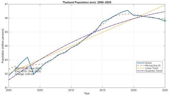
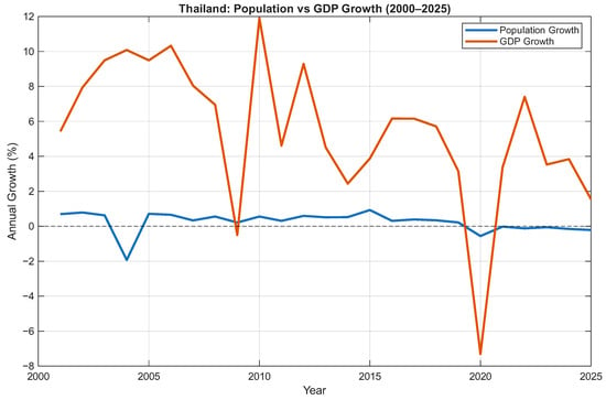
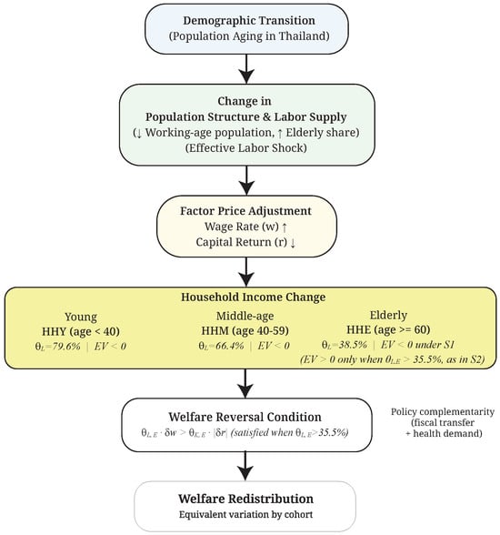
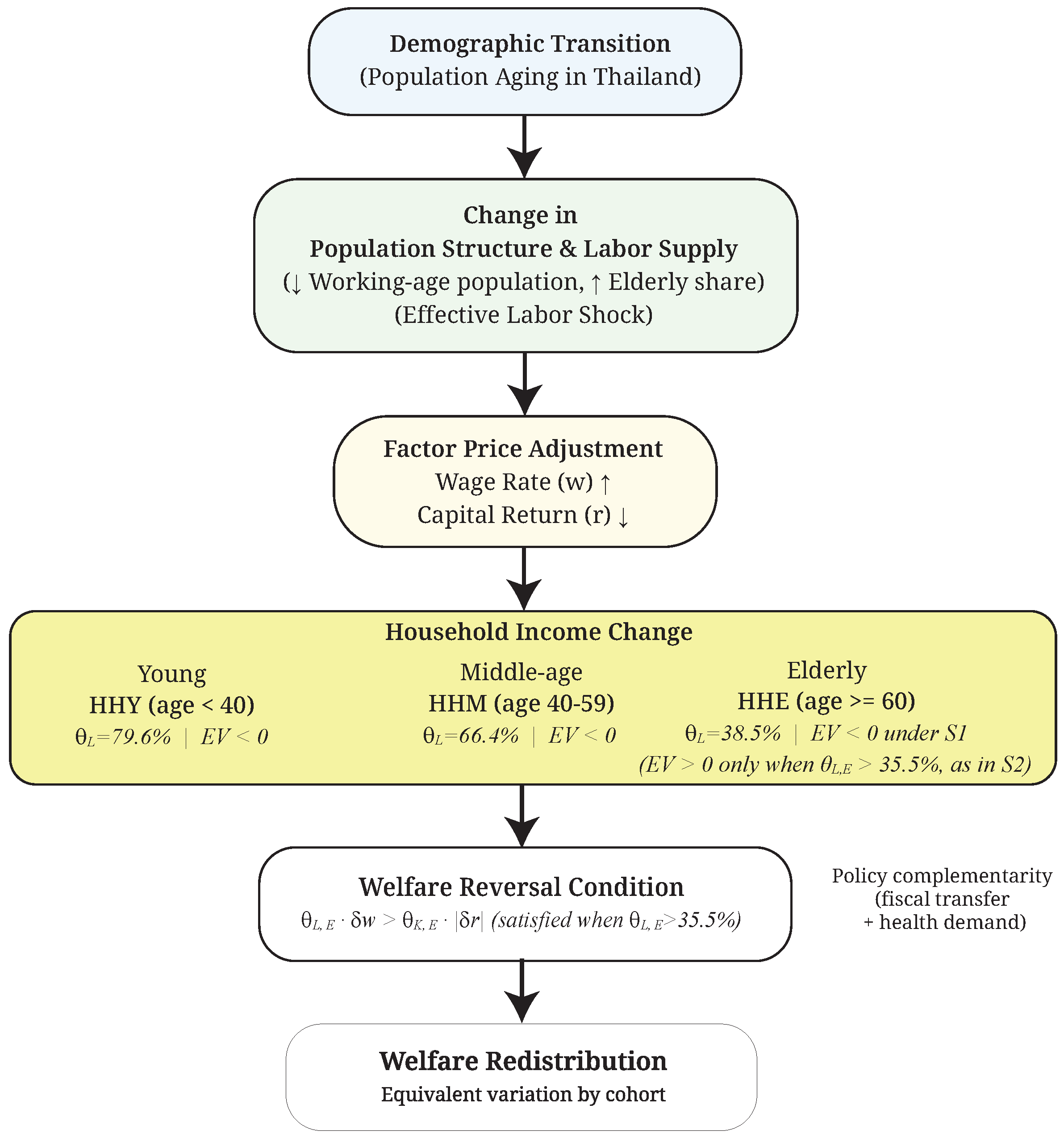
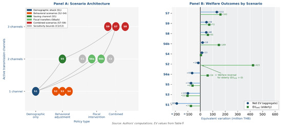
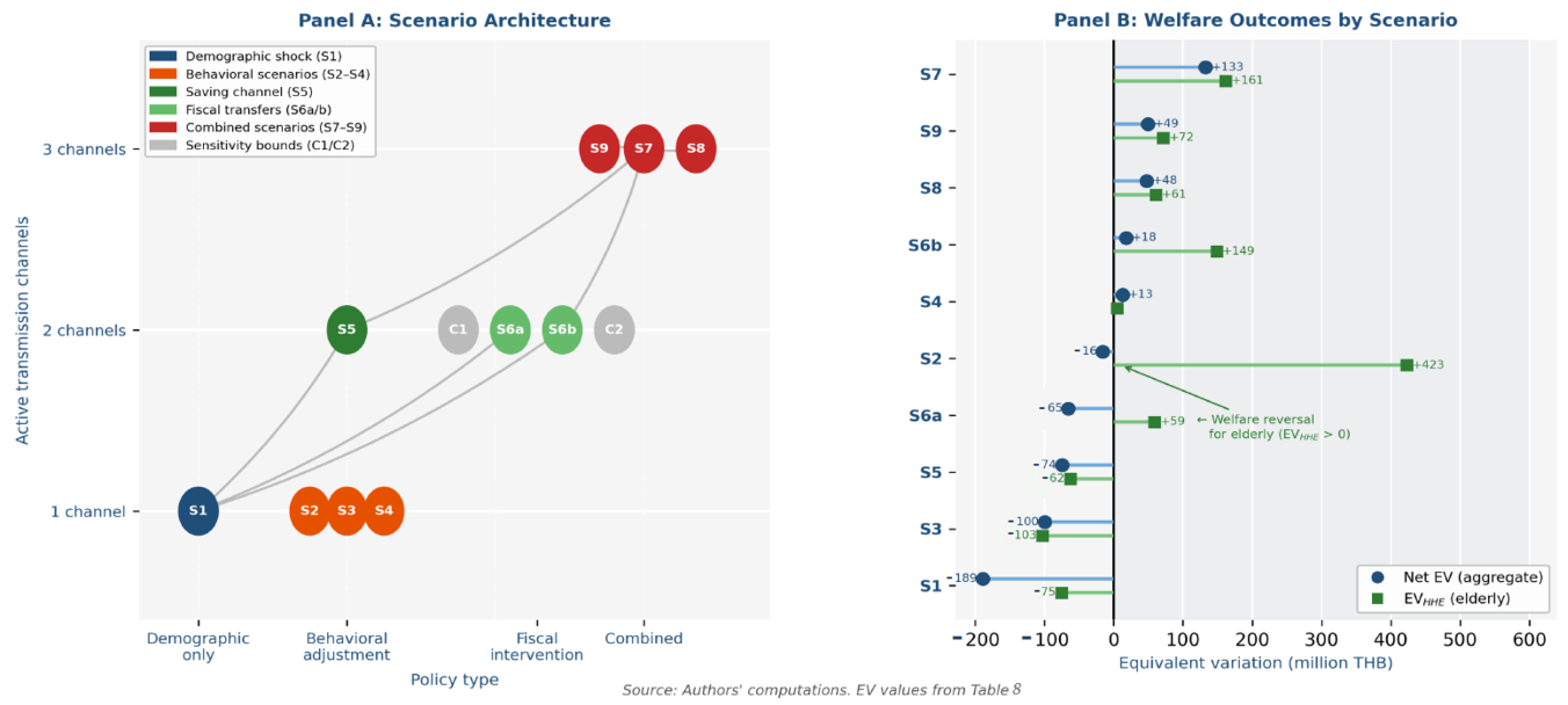
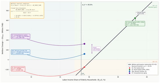
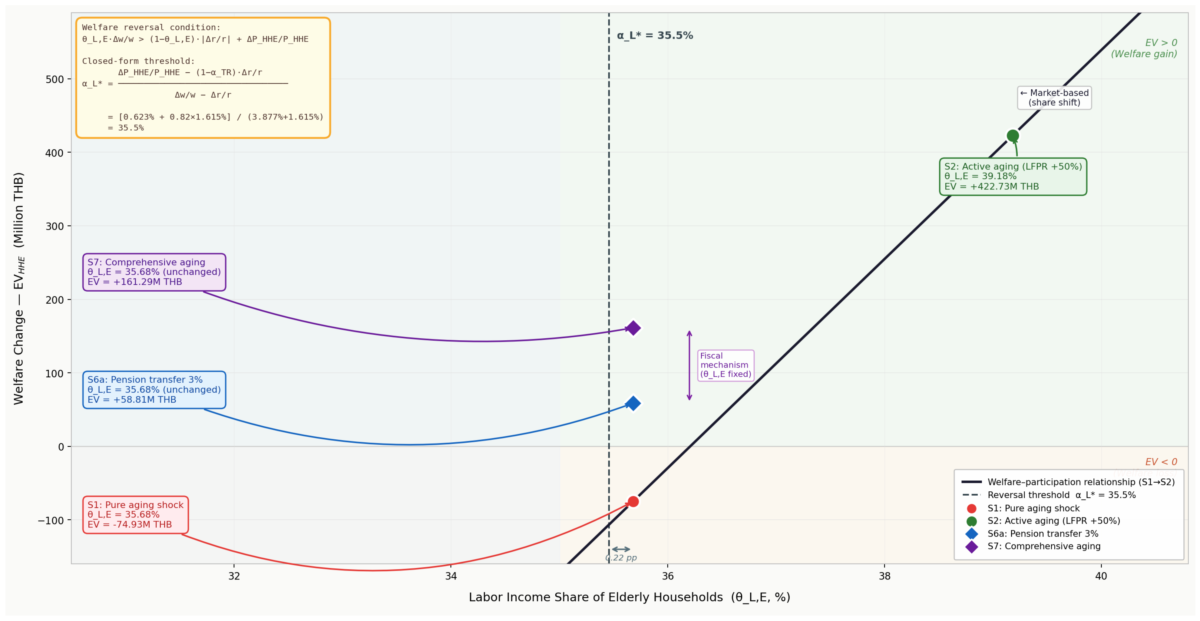

Disclaimer/Publisher’s Note: The statements, opinions and data contained in all publications are solely those of the individual author(s) and contributor(s) and not of MDPI and/or the editor(s). MDPI and/or the editor(s) disclaim responsibility for any injury to people or property resulting from any ideas, methods, instructions or products referred to in the content. |
© 2026 by the author. Licensee MDPI, Basel, Switzerland. This article is an open access article distributed under the terms and conditions of the Creative Commons Attribution (CC BY) license.