


Abstract
This work presents a reproducible YOLO-based pipeline for bottle detection in sandy environments, emphasizing dataset integrity, leakage-free evaluation, and deployment-oriented model selection. A one-class dataset of 1585 images and 3167 annotated bottles was audited to identify annotation-format defects and near-duplicate contamination between training and validation partitions. Sequence membership was reconstructed through perceptual-image similarity and used to assign complete image components to a sequence-aware train/validation split, eliminating the near-duplicate pairs found in the initial random partition. A controlled ablation holding model, seed, and corrected labels fixed showed that the random split reports 0.040 higher mAP@0.5:0.95 than the sequence-aware split (0.787 vs. 0.747), quantifying the leakage risk directly rather than only asserting it. Five YOLO configurations were then benchmarked under three independent seeds each; the observed mAP@0.5:0.95 differences among models (0.004–0.008) were small in absolute magnitude and, given only three seeds per model, are interpreted descriptively rather than as evidence of statistical equivalence or significance, so yolo11n_bottle was selected through a joint accuracy-parity, compactness, and exportability criterion (precision 0.982, recall 0.985, mAP@0.5 0.992, mAP@0.5:0.95 0.748), using approximately ten times fewer parameters than the largest configuration and producing a 5.2 MB checkpoint. ONNX export preserved detection geometry closely (100% count agreement, mean matched IoU ), without meeting strict metric-parity tolerances. A stratified sample of 108 frames from operational RealSense BAG footage was manually annotated by an independent reviewer and evaluated quantitatively: mAP@0.5 remained close to the internal validation figure (0.927 vs. 0.992), while mAP@0.5:0.95 fell substantially (0.483 vs. 0.747), revealing a localization gap between the curated benchmark and operational conditions that this manuscript reports transparently. Together, these results show that dataset auditing, sequence-aware partitioning, multiseed benchmarking, and manually annotated operational evidence are each necessary to interpret a detection benchmark built from continuous video acquisition, providing a traceable, reproducible workflow for selecting and evaluating compact visual-perception models for resource-constrained environmental applications.
1. Introduction
Reliable benchmarking of object detectors depends on the integrity of the dataset used to train and validate them. When a reported benchmark is built on a dataset with annotation defects, near-duplicate samples, or an uncontrolled train/validation split, the resulting accuracy figures can substantially overstate real detector performance rather than reflect it.
This vulnerability is particularly acute for datasets derived from video sequences. Consecutive or near-consecutive frames extracted from the same recording session are visually near-identical, and a naive random train/validation split routinely assigns near-duplicate frames to both partitions, inflating validation metrics through leakage rather than genuine generalization. This risk applies broadly to visual datasets built from recorded video rather than independently sampled images, which is increasingly common in applied computer-vision projects that rely on onboard or handheld RGB-D sensors, such as Intel RealSense cameras, to collect training data.
A further practical requirement, beyond raw accuracy, is deployment-oriented model selection: choosing a detector configuration is rarely a matter of maximizing a single accuracy metric. It requires balancing accuracy against model compactness, parameter count, and exportability to portable inference formats, since the most accurate configuration in a benchmark table is not necessarily the most suitable one to carry forward toward a resource-constrained target.
This paper addresses these three issues, dataset integrity, leakage-free evaluation, and deployment-oriented selection, through a reproducible workflow for one-class bottle detection using YOLO-family object detectors. The dataset used here is drawn from a beach-cleaning robot project [1,2], in which visual detection of discarded plastic bottles on sandy terrain provides the motivating application; the robot platform is treated strictly as the application context for the visual perception subsystem, not as the object of evaluation. Working from this dataset, the manuscript reports a dataset audit that identifies and corrects an annotation-format defect and near-duplicate train/validation contamination, a sequence-aware, leakage-free re-partitioning strategy whose effect on reported accuracy is directly quantified through a controlled ablation, a multiseed benchmark of five YOLO configurations under the corrected split, and a compact-model selection with controlled-latency and export-format analysis of the resulting detector, yolo11n_bottle (Section 6.2). The reported evidence is offline in scope: held-out validation-image inference, recorded-sequence (RealSense BAG) replay, and a manually annotated operational sample drawn from that same recording, rather than closed-loop robot operation, which remains future work. This offline scope applies to every result in this manuscript and is not restated section by section.
The main contributions are as follows:
- Dataset auditing, visual-sequence reconstruction, and leakage-free train/validation partitioning for a one-class bottle-detection dataset, with a controlled ablation quantifying the leakage effect of the initial random, frame-level split against the corrected sequence-aware split.
- A multiseed benchmark of five YOLO configurations on the corrected split, with yolo11n_bottle selected through an explicit accuracy-parity–compactness–exportability trade-off rather than by mAP@0.5:0.95 alone, supported by a controlled single-frame latency benchmark and an ONNX export-parity analysis.
- Offline evaluation of the selected detector through held-out validation-image inference, unannotated RealSense BAG replay of a recorded RGB sequence, and a manually annotated, human-verified 108-frame operational sample drawn from that same recording.
- A deployment-oriented export analysis of the selected detector (TorchScript, ONNX FP32/FP16), with TensorRT limitations explicitly reported.
2. Related Work
2.1. Object Detection and YOLO-Based Perception
Visual object detection is a central component of many robotic perception pipelines because it converts image streams into spatial hypotheses about task-relevant objects. Two-stage detectors such as Faster R-CNN established strong detection accuracy through region proposal and classification stages [3]. For robotic and embedded applications, however, single-stage detectors are often attractive because they reduce the complexity of the inference pipeline and can provide lower latency.
YOLO-family detectors are representative single-stage methods. Earlier single-stage detectors such as SSD also showed the importance of unified detection architectures for efficient inference [4]. The original YOLO formulation reframed object detection as a single regression problem, predicting bounding boxes and class probabilities directly from full images in one forward pass and enabling real-time detection at the time of its introduction [5]. YOLOv3 emphasized a practical speed–accuracy trade-off for real-time object detection [6], while YOLOv4 further explored architectural and training improvements to improve accuracy at real-time speed [7]. More recently, YOLOv8 has been applied to detection tasks well beyond litter and environmental monitoring, for example, to human motion detection and movement measurement on mobile devices in combination with R-CNN and augmented reality [8], illustrating that the same detector family is being adapted across markedly different application domains rather than remaining specific to any one of them. Comparative, multi-model evaluation is likewise common practice beyond object detection: a recent comparison of Random Forest and support-vector-machine classifiers for food-image recognition [9] follows the same general principle applied in the present manuscript, benchmarking several models on a common task rather than reporting a single configuration, although that work addresses image classification rather than object detection and does not consider dataset leakage or split design. The present work follows this practical, application-oriented motivation: the detector is not evaluated as an isolated benchmark only, but as part of a visual perception subsystem intended for later deployment-oriented use.
2.2. Litter, Waste, and Bottle Detection
Waste detection in unconstrained outdoor scenes remains challenging because objects may be small, partially occluded, deformed, reflective, or visually similar to the background. The TACO dataset was introduced to support litter detection and segmentation in context, including diverse real-world scenes and manually annotated waste instances [10]. Marine-debris and underwater-trash studies similarly emphasize the need for domain-specific datasets and visual detection pipelines for waste-like objects [11,12,13]. Floating-plastic detection studies using vessel-mounted cameras also show that outdoor litter detection depends strongly on acquisition conditions and visual context [14]. These works highlight a common limitation for trash detection: larger and more diverse annotations are needed for robust deployment in the wild.
Closer to the present target class, prior work has applied instance segmentation specifically to plastic bottles as a waste category, using a small manually annotated dataset and transfer learning from a Mask R-CNN model pretrained on MS COCO [15]. That study reports strong segmentation performance on its own dataset, but it uses a different task formulation (instance segmentation rather than bounding-box detection), a different model family, and a different sensor and annotation protocol than the one-class YOLO detection benchmark reported here, so its metrics are not directly comparable to the present results.
The accuracy–compactness–latency trade-off motivating the present model-selection criterion is not specific to beach litter: a compact YOLOv8 detector has similarly been benchmarked for real-time recyclable-material detection inside reverse vending machines, trained on a combination of a public dataset and a study-specific dataset, and compared against several YOLO variants under real-time operational constraints [16]. That operational-recycling setting shares the present work’s emphasis on compact, real-time YOLO inference for bottle-like targets, but it differs in acquisition context: reverse vending machines present controlled indoor lighting and a constrained object presentation, whereas the present sandy-beach domain introduces variable outdoor illumination, a textured and partially occluding sand background, and robotic (rather than fixed-station) image acquisition, all of which motivate the dataset-auditing and sequence-aware evaluation steps described in Section 6.2 and are not addressed by that or other adjacent waste-detection studies.
Beach environments add additional difficulty because sand texture, shadows, and object burial can reduce visual contrast. The present study therefore focuses on a narrower and traceable task: one-class bottle detection using a project-specific dataset and offline replay of recorded RealSense imagery. This scope allows the detector behavior to be evaluated consistently before further application-level testing is attempted.
2.3. Dataset Integrity, Annotation Quality, and Leakage-Free Evaluation
The reliability of a reported detection benchmark depends not only on the detector but on the integrity of the dataset and split used to evaluate it. Barz and Denzler showed that near-duplicate images shared between training and test partitions in CIFAR-10 and CIFAR-100 inflate reported classification accuracy, and that purging such duplicates raises the measured error rate by roughly 9–14% [17]. A comparable pattern has been documented outside image classification: in large-scale geospatial building-footprint datasets, near-duplicate and augmented-duplicate images shared between training and validation splits were found to affect the large majority of one benchmark’s validation images, together with a corresponding drop in accuracy on genuinely unseen data [18]. Beyond duplication, annotation quality itself measurably affects object-detection and instance-segmentation performance: incorrect class labels, missing annotations, and localization noise each degrade mAP, with incorrect labels producing the largest effect [19]. Dedicated noise-resistant training and annotation-refinement methods have also been proposed to mitigate label and bounding-box noise during detector training [20,21]; the present work does not implement these training-time correction methods and instead performs an explicit dataset audit and correction step prior to training.
These findings motivate treating dataset auditing and leakage-free evaluation as a methodological prerequisite rather than an optional check. Consistent with this view, the dataset used in this manuscript was audited before the final benchmark, a spurious sixth label column was identified and corrected, and the train/validation partition was rebuilt as a sequence-aware, leakage-free split to remove near-duplicate-frame contamination between partitions (Section 6.2).
Near-duplicate detection for this purpose can be approached with several families of methods, including perceptual hashing, CNN-embedding similarity, and structural pixel-level metrics such as SSIM, and the choice among them is not neutral to the resulting split. This manuscript compares three perceptual-hash variants empirically rather than selecting one by convention: a average hash (aHash), a difference hash (dHash), and a DCT-based perceptual hash (pHash), all applied at the same Hamming-distance threshold of 5 to the same image pool (Section 6.2.2). The three methods disagree on which specific image pairs they flag, consistent with each emphasizing a different low-level image statistic (average intensity for aHash, local gradient direction for dHash, frequency-domain content for pHash), which argues against treating any single hash family as a uniquely correct leakage detector. Average hash was retained as the primary method because it produced the most conservative (largest) near-duplicate estimate at the chosen threshold among the three, so a split built to satisfy it is, by construction, at least as strict with respect to the other two. A structural-similarity (SSIM) check was additionally used, not as an alternative deduplication criterion, but to test whether the shared sandy background specifically, rather than genuine frame duplication, could explain residual cross-split similarity at larger Hamming distances (Section 8). A comparison against CNN-embedding-based near-duplicate detection, which can capture higher-level semantic similarity that pixel- and hash-based methods miss, was not performed in this work and is identified as a direction for further methodological comparison.
2.4. RealSense Replay and Deployment-Oriented Considerations
RGB-D sensors such as Intel RealSense cameras are commonly used in robotics because they support synchronized visual acquisition and recorded-sequence replay [22]. The Intel RealSense SDK supports recording a streaming session to a .bag file and later loading that file for offline playback [23], and the SDK’s official Python examples illustrate how recorded .bag files can be loaded and processed frame by frame through the same pipeline API used for a live device [24]. In this manuscript, RealSense BAG replay is used as an offline validation mechanism following this pattern: each recorded RGB frame is processed by the selected detector, and detection counts, confidence, and timing are logged. This improves repeatability, but it does not measure navigation, collection, or other closed-loop robot behavior.
Embedded deployment often requires converting trained models into formats that can be loaded efficiently outside the original training script. Efficient neural-network families for mobile vision, such as MobileNet and MobileNetV2, illustrate the broader need to balance model capacity, speed, and deployment constraints [25,26]. ONNX provides an open representation intended for model interoperability across frameworks, tools, runtimes, and compilers [27]. TorchScript provides a serializable PyTorch representation that can be loaded and executed outside ordinary Python training code paths [28]. TensorRT is designed to optimize and accelerate trained models on NVIDIA GPUs with support for reduced precision and hardware-specific inference optimizations [29]. An empirical benchmark of deep object-detection models converted for two embedded co-processor platforms found that many models could not be converted or executed without modification, that measured inference time depended strongly on model architecture and target hardware, and that co-processor acceleration relative to CPU-only inference varied by roughly 5× to more than 30× across models [30]; this reinforces that export success and measured latency are runtime- and hardware-dependent outcomes rather than guaranteed properties of a given export format. Recent edge-device benchmarking work further reinforces that export format, runtime, and target hardware can substantially affect measured inference behavior [31]. These tools and findings motivate the export analysis reported in this work, while the TensorRT result is explicitly limited by the absence of the tensorrt module in the Windows environment used for export, and target-hardware deployment (e.g., on a Jetson-class device) is treated as future work rather than a reported result.
2.5. Beach-Cleaning and Environmental Robotics Context
Robotic platforms for beach and litter cleaning have been explored both as engineering-design efforts and, more recently, as integrations with real-time visual detection. The robot platform used in this project, Beach-O, was previously described as a mechanical-design and preliminary-validation effort [1,2]; the present manuscript narrows its scope to an offline evaluation of the visual-perception subsystem and does not reuse those prior outputs as new experimental evidence.
Recent published work has reported an autonomous beach-cleaning robot prototype that applies a real-time YOLO-family detector for waste classification, illustrating a broader application trend toward integrating visual detection into beach-cleaning platforms [32]; this reference is cited only for that contextual trend, since its full text was not accessible beyond the published abstract and bibliographic metadata, and it is not used as a basis for numerical or hardware-level comparison with the present results. Environmental-monitoring studies further motivate the underlying problem: accelerated beach-litter survey protocols have been proposed to make pollution-hotspot monitoring more practical at heavily used urban beaches [33], reinforcing that visible beach litter, including bottles, is a persistent monitoring and mitigation target independent of any particular robotic platform.
Beyond beach-specific platforms, autonomous litter-picking robots have combined deep-learning-based detection with soft robotic manipulation for roadside litter collection [34], and a comparative benchmarking study of deep object detectors—including YOLOv5 variants under mobile-device constraints—has been reported specifically for litter detection in natural environments [35]. These studies illustrate a broader research trend toward integrating YOLO-family detectors into environmental and litter-collection robotics, but none of them evaluate the present dataset, sensor, or robot platform. They are cited here only to situate the present offline perception evaluation within that broader context, and not as evidence supporting closed-loop validation, navigation, or physical collection by the present system.
3. Application Context and Visual Perception Pipeline
The application context for this study is a beach-cleaning robot equipped with visual sensing for bottle detection; the robot supplies the operating scenario for the visual perception subsystem evaluated in this manuscript. The perception pipeline processes RGB imagery, detects bottles, records bounding boxes and confidence values, and prepares model artifacts for deployment-oriented export.
The Beach-O robot platform was previously described as a mechanical-design, prototype-development, and preliminary-validation effort: the Convergencia Mecatrónica 2024 book chapter reported the design proposal, mechanical concept, and preliminary validation, and the ICECET 2025/IEEE paper reported the design and implementation of the autonomous prototype [1,2]. Those prior works are used here only as platform background and are not reused as new experimental evidence; the present manuscript instead reports the offline YOLO perception-subsystem evaluation, dataset audit, benchmark, RealSense BAG replay, and embedded-export analysis summarized throughout Section 6.2, Section 6.3, Section 6.4, Section 6.5, Section 6.6, Section 7 and Section 8.
Figure 1 shows the physical prototype that defines the application context for the study; the visual perception subsystem evaluated in this manuscript was developed for this platform.
Figure 1.
Beach-cleaning robot prototype used as the application context for the YOLO-based visual perception subsystem.
Figure 2 summarizes the evaluated perception flow from RGB acquisition to detector outputs, offline logging, replay products, and export formats.
Figure 2.
Architecture of the YOLO-based visual perception subsystem evaluated in this work, from RealSense RGB acquisition to the yolo11n_bottle detector, detection outputs, offline logging and replay products, and deployment-oriented export formats.
The reported results comprise dataset validation, held-out validation-image inference, RealSense BAG replay, and deployment-oriented export analysis; together they constitute an offline evaluation of the visual perception subsystem rather than a claim of closed-loop robot behavior.
4. YOLO Perception System
The detector was formulated as a one-class object detector for bottles, trained and benchmarked using the Ultralytics YOLO implementation [36]. The valid class mapping used in the final experimental pipeline is class 0: bottle. The perception system uses the selected yolo11n_bottle detector for held-out validation-image inference, RealSense BAG replay, and deployment-oriented export analysis.
4.1. Dataset Construction and Annotation Protocol
The dataset was prepared as a YOLO-format object-detection dataset for a single target class. Each annotation file follows the normalized YOLO bounding-box format:
where x_center, y_center, width, and height are normalized with respect to the image width and height. Positive images contain at least one bounding box for class 0. Negative images are represented by existing empty .txt label files. Empty label files are valid in YOLO workflows and indicate images with no bottle instances; this distinction prevents negative images from being misinterpreted as missing annotations.
Consistent with evidence that annotation quality and dataset integrity directly affect measured detection performance [19], the dataset audit checked image counts, label counts, total bounding boxes, empty labels, images without labels, orphan labels, invalid classes, and coordinates outside the normalized range. System or editor artifacts such as ._*.txt files were ignored during the audit so that they did not affect annotation integrity checks. Table 1 summarizes the annotation and audit protocol. Figure 3 summarizes the annotation workflow, and Figure 4 shows representative dataset examples used in the one-class detection task.
Table 1.
Dataset annotation and audit protocol.
Figure 3.
Dataset preparation and YOLO annotation workflow. Positive images contain normalized bottle bounding boxes, whereas negative images are represented by empty label files and were preserved during the audit.
Figure 4.
Representative examples from the audited bottle-detection dataset, including positive and negative images used for one-class YOLO training and validation: (a–c) positive examples with a detected bottle; (d) a negative example without a detected bottle; (e,f) additional dataset examples with a detected bottle.
The preliminary dataset version was audited before the final benchmark. This audit identified two correctable defects: (i) a subset of label files carried a spurious sixth column (a leftover confidence score from an earlier inference pass) that is not part of the standard YOLO label format and is silently dropped by common training pipelines, and (ii) an initial random image-level train/validation partition allowed a small number of exact-duplicate images to appear on both sides of the split. The dataset was then curated by correcting the label-format defect and rebuilding the train/validation partition with the sequence-aware strategy described in Section 6.2. All main results reported in this manuscript use this final sequence-aware split.
4.2. Dataset Audit
The final dataset audit identified 1585 images, 1585 label files, and 3167 annotated bounding boxes across the sequence-aware training and validation splits (Section 6.2). Table 2 summarizes the audited dataset. Missing labels and orphan labels were both zero in the final audit, and no label file retained the six-column confidence-score defect described above.
Table 2.
Dataset summary for the final sequence-aware, leakage-free split used in the final benchmark.
4.3. YOLO Benchmark Models
Five YOLO benchmark runs were evaluated: yolov8n_bottle, yolov8s_bottle, yolov8m_bottle, yolo11n_bottle, and yolo11s_bottle, on a sequence-aware, leakage-free validation configuration (Section 6.2). The final model-selection criterion was a trade-off between accuracy (mAP@0.5:0.95, precision, recall), model compactness (parameter count, checkpoint size), exportability, and real-time offline performance under RealSense BAG replay, rather than mAP@0.5:0.95 alone.
yolov8m_bottle achieved the highest mAP@0.5:0.95 among the benchmarked models, but by a marginal margin. The selected model, yolo11n_bottle, matched or exceeded yolov8m_bottle on precision and recall while requiring roughly 10× fewer parameters and producing substantially smaller deployment artifacts; it is therefore used for held-out validation-image inference, RealSense BAG replay, and deployment-oriented export analysis.
5. Methods: Offline Evaluation and Deployment Pipeline
The final experimental pipeline is organized in the data_jcr directory. It includes dataset checks, model training, benchmark validation, test-image prediction, RealSense BAG replay, embedded export, and article-table/figure generation. The reported values come from generated CSV files and figures. As shown in Figure 5, the methodology is organized into dataset preparation, dataset audit, benchmark/model selection, offline replay/export, and future target-system validation.
Figure 5.
Methodological pipeline used in the present study. The workflow separates dataset preparation, dataset audit (including the six-column label check and the sequence-aware split), YOLO benchmarking with yolo11n_bottle as the selected model, offline validation through test-image prediction and RealSense BAG replay, and embedded export analysis. Future target-system validation is shown only as a subsequent research step and is not claimed as a result of this manuscript.
5.1. Dataset Audit and Benchmark Inputs
The dataset audit verifies image counts, label counts, bounding-box totals, empty label files, missing labels, and orphan labels before the benchmark results are interpreted. This step is important because the study uses a one-class bottle detector, and unlabeled negative images can be valid only when they are intentionally represented by empty label files. The audit also confirmed that no label file retained the spurious six-column confidence-score defect found during preliminary dataset review, and that the final sequence-aware split (Section 6.2) contains no exact-duplicate images shared between training and validation. The final dataset summary contains 1585 images, 1585 label files, and 3167 bounding boxes (1267/318 train/validation split).
5.2. Model Benchmarking
Each benchmark model is trained and validated using the frozen data_jcr configuration on a sequence-aware, leakage-free train/validation split (Section 6.2). The final comparison uses the validation metrics exported by the benchmark script, including precision, recall, mAP@0.5, mAP@0.5:0.95, preprocessing time, inference time, postprocessing time, and validation time. The benchmark table is sorted by mAP@0.5:0.95 in descending order. yolov8m_bottle obtains the highest mAP@0.5:0.95 by a marginal margin; the selected detector is yolo11n_bottle, chosen through a trade-off between accuracy, model compactness, parameter count, exportability, and real-time offline performance.
5.3. Held-Out Validation-Image Inference and Qualitative Inspection
The offline validation path has two stages. First, the selected model is applied to the validation/test image folder, producing annotated images, per-image summaries, and detection-level CSV logs. The annotated images are used only for qualitative inspection and for visual examples in the article; quantitative validation metrics are taken from the benchmark validation CSV files.
5.4. RealSense BAG Data Acquisition
The RealSense BAG sequence used for offline replay was recorded on a controlled sandy-terrain test area at Zigzag, the interactive science and technology center associated with the COZCyT science-dissemination ecosystem in Zacatecas, Mexico [37,38]. This setting was used to emulate the visual conditions of the beach-cleaning scenario, including a sandy background and a single bottle target. During acquisition, the platform followed a zigzag traversal pattern around the target bottle, intended to introduce visual variability in distance, viewing angle, relative position, sandy-background appearance, and partial occlusion where present. An Intel RealSense camera recorded the corresponding RGB stream to a single .bag file using the SDK’s record-and-playback mechanism [23]. This recorded file was subsequently used as a fixed input for offline replay, allowing the same visual sequence to be reprocessed repeatedly and detections, confidence, inference time, and detection geometry to be logged consistently. The complete RealSense BAG file is included in the archived dataset release and documented through the public dataset repository cited in the Data Availability Statement. This acquisition and replay procedure evaluates the offline visual-perception subsystem; it does not constitute validated autonomous navigation, closed-loop robot control, or validated physical waste collection.
5.5. RealSense BAG Replay
Second, the same model is applied to the recorded RealSense BAG sequence, following the record-and-playback workflow and Python playback pattern documented for the Intel RealSense SDK [23,24]. The recorded sequence corresponds to the COZCyT sandy-terrain zigzag acquisition protocol described above (Section 5.4). During BAG replay, each RGB frame is processed offline, and the pipeline stores frame index, timestamp, number of detections, maximum confidence, inference time, and detection geometry. The BAG summary reports detection activity and timing under repeated replay of the same visual sequence, constituting the recorded-sequence evaluation of the acquisition described above.
5.6. Deployment-Oriented Model Export
The deployment-oriented export path exports the selected best.pt checkpoint to portable formats: TorchScript [28] and ONNX FP32/FP16 [27]. TorchScript, ONNX FP32, and ONNX FP16 were successfully generated. TensorRT FP16 and TensorRT INT8 were attempted as planned deployment targets using the NVIDIA TensorRT toolchain [29], but they are reported as failed in the current Windows environment because the tensorrt Python module was not available. Therefore, no successful TensorRT deployment claim is made. This mirrors the broader observation that portable model export and acceleration success are runtime- and hardware-dependent outcomes rather than guaranteed properties of a given format [30].
6. Experimental Configuration
All final metrics reported in this manuscript were generated from the data_jcr pipeline using the curated dataset and its final sequence-aware split. The dataset summary, benchmark metrics, BAG summary, embedded-export summary, and article-ready tables were read from the generated CSV files in the sequence-split dataset summaries and final article-asset directories.
The benchmark was sorted by mAP@0.5:0.95 in descending order and evaluated on a sequence-aware, leakage-free train/validation split (Section 6.2). yolov8m_bottle obtained the highest mAP@0.5:0.95, by a marginal margin; the selected model was yolo11n_bottle, chosen through a trade-off between accuracy, model compactness, parameter count, exportability, and real-time offline performance. The RealSense BAG file used for offline replay was the recorded sequence 20241128_133505.bag, stored in the project data directory. A confidence threshold of 0.50 was used in the final BAG summary. Figure 6 and Table 3 summarize the experimental flow and final protocol.
Figure 6.
Experimental flow from dataset audit, through the sequence-aware split, to model selection (yolo11n_bottle), offline replay, and embedded export analysis. The future target-system validation branch is included only to show the next research step and is not part of the reported results.
Table 3.
Experimental protocol summary.
Article-ready tables and figures were generated by the table/figure generation script in data_jcr/scripts. The figures follow a clean journal style with labeled axes, 300 dpi export, and direct correspondence to the final CSV summaries. The qualitative detection panel was generated from annotated outputs of the test-image prediction script, and its source-image provenance is stored with the final article tables.
6.1. Training Protocol and Training-Time Measurement
All five benchmarked models (yolov8n_bottle, yolov8s_bottle, yolov8m_bottle, yolo11n_bottle, yolo11s_bottle) were trained on the sequence-aware split (Section 6.2) with the same recorded configuration: Ultralytics 8.4.80 with PyTorch 2.5.1+cu121, image size 640, a maximum of 100 epochs with an early-stopping patience of 20, device index 0, a fixed random seed of 42, deterministic mode enabled, zero dataloader workers, and Ultralytics AutoBatch (batch = −1), which selects a batch size automatically per model from available GPU memory. Data augmentation used Ultralytics’ documented default pipeline without custom overrides, summarized in Table 4 for exact replication. This configuration was held identical in everything that was recorded; as detailed next, the one exception is the effective batch size resolved by AutoBatch, which was not logged and cannot be confirmed as identical across models.
Table 4.
Data augmentation parameters used for all training runs (Ultralytics default pipeline, no custom overrides).
Zero dataloader workers (workers = 0) was used to keep data loading single-threaded and execution order deterministic on the Windows/GPU workstation described below; this choice favors run-to-run reproducibility over maximum data-loading throughput and may therefore not minimize wall-clock training time relative to a multi-worker configuration. Because Ultralytics AutoBatch was enabled, the effective batch size may also differ across models depending on GPU memory availability at run time; the resolved per-model batch size was not captured by the original training logs and could not be reliably recovered retrospectively without retraining, which was outside the scope of this revision. This is reported here as a methodological limitation rather than omitted silently, and it is restated in Section 8: complete comparability of training conditions across the five models should not be assumed on this specific point, even though every other recorded element of the protocol was identical.
Training was performed on a Windows 11 Pro 64-bit workstation equipped with an AMD Ryzen 7 5800X CPU, 64 GB of RAM, and an NVIDIA GeForce RTX 4060 Ti GPU with 8 GB of dedicated VRAM. This hardware description is provided to contextualize the training times reported in Table 5, which should be interpreted as platform-specific computational-cost measurements rather than hardware-independent properties of the detector architectures.
Table 5.
Training time for the five benchmarked models on the sequence-aware, leakage-free split.
Training time was measured with Python’s perf_counter(), started immediately before and stopped immediately after the complete model.train(...) call for each model. This training-time figure therefore includes Ultralytics’ own end-of-training validation and plotting overhead in addition to the epoch loop, and it is distinct from the controlled per-frame inference latency reported in Section 7.8; the two should not be interpreted as the same quantity. Table 5 reports the completed epochs, total training time, and mean time per completed epoch for each model. Early stopping (patience 20) triggered before the 100-epoch budget for yolov8n_bottle, yolov8s_bottle, and yolov8m_bottle; yolo11n_bottle and yolo11s_bottle completed the full 100-epoch budget. Mean time per epoch is therefore computed over each model’s own completed-epoch count, not over a common denominator.
6.2. Sequence-Aware Train/Validation Split
After the preliminary dataset version had been corrected for YOLO label-format defects, an initial random frame-level train/validation split was inspected for visual leakage. This inspection showed that near-duplicate video frames crossed the two partitions: a perceptual average-hash check (16 × 16 grayscale, 256-bit) showed that 128 of 318 validation images (40%) were hash-identical to a training image, and 220/318 (69%) fell within a Hamming distance of 5 bits. Pixel-level mean-squared error confirmed these pairs were near-identical frames (MSE 1.7–40.2 on a 0–255 scale), consistent with consecutive or near-consecutive extraction from continuous video rather than independently sampled scenes. Training on such a split inflates validation metrics because the model is effectively evaluated on samples it has already seen a near-copy of, consistent with near-duplicate leakage effects documented in other visual benchmarks [17,18].
Because the dataset carries no ground-truth video- or sequence-identifier metadata, sequence membership was reconstructed directly from visual content. All 1585 images (train and validation pooled) were hashed as above, and an undirected graph was built with an edge between any two images at Hamming distance ; each connected component was treated as one indivisible sequence. The threshold was chosen empirically: at distance , the largest component contained 101/1585 images (6.4%), while at distance , a single component absorbed roughly one third of the dataset (a shared static background bridging unrelated frames), which was rejected as unworkable. Components were then assigned whole to train or validation with a deterministic greedy packing (largest components first) targeting the original 80/20 image-count ratio (1267/318) so that no sequence straddled the split boundary.
The resulting final sequence-aware split was re-checked with the same near-duplicate procedure: the minimum Hamming distance between any validation image and its nearest training neighbor rose from 0 to 6, and the 220 previously flagged near-duplicate pairs dropped to 0. Residual matches at a distance of 6–10 were verified to have pixel MSE of 22–690 (5–30× higher than the true near-duplicates removed), confirming they share only the common beach background and not frame identity. This final sequence-aware split is the one used for all results reported in Section 7.3.
6.2.1. Random-vs.-Sequence-Aware Split Ablation
To isolate the effect of the train/validation split from the effects of the annotation-format correction and dataset curation described above, a controlled ablation trained yolo11n_bottle twice, with an identical model, seed (42), image size, epoch budget, and corrected (six-column-defect-free) label set, differing only in which split it used: (a) the original random, frame-level split, or (b) the final sequence-aware split. Both runs used the same checkpoint architecture and training configuration described in Section 6.1. This ablation directly answers the question of how much of the benchmark’s headline accuracy is attributable to split design alone, holding data quality and architecture fixed. Results are reported in Section 7.1.
6.2.2. Hash-Threshold Sensitivity
The Hamming-distance threshold of 5 used to define near-duplicate clusters (Section 6.2) was chosen as an operational design boundary rather than derived from a single universally correct value. To characterize how sensitive the resulting split composition is to this choice, the same average-hash clustering procedure was repeated at every integer threshold from 3 to 7, recording the number of validation images that would remain cross-split-adjacent to a training image, the number of cross-split edges, and the number of connected components spanning both partitions. As a secondary check, two alternative perceptual-hash methods, difference hash (dHash) and DCT-based perceptual hash (pHash), both , were applied at the same threshold of 5 to test whether the choice of hashing method itself changes the qualitative conclusion. Results are reported in Section 7.2.
6.3. Multiseed Benchmark Protocol
To assess whether the benchmark ranking in Section 7.3 is stable across training stochasticity, each of the five models was retrained on the same sequence-aware split under three independent random seeds (42, 123, 2026), holding every other training argument in Table 4 and Section 6.1 fixed. This treats the training seed, not the image, as the unit of repeated observation: each of the three runs per model is an independent full training-and-validation cycle on the same fixed 1267/318 split, so the resulting variability reflects training stochasticity (weight initialization, data shuffling order, and CUDA non-determinism where applicable) rather than sampling variability across images. Results are reported as the mean ± standard deviation over the three seeds in Section 7.4.
6.4. Controlled Latency Protocol
The single-frame BAG-replay timing reported for yolo11n_bottle in Section 7.6 and the preliminary yolov8s_bottle figure retained for historical context both originate from sequential model.predict() calls during BAG replay without a dedicated warm-up phase, repeated timing, or explicit GPU synchronization, and they are not directly comparable across models trained under different dataset versions. To obtain a directly comparable, controlled figure for all five models, a dedicated single-frame latency benchmark was run for each final best.pt checkpoint on the same GPU: model weights were loaded once, a fixed number of warm-up inferences discarded, followed by repeated timed single-image inference calls with explicit CUDA synchronization before and after each call, at image size 640, FP32 precision, batch size 1. Both end-to-end latency (preprocessing, forward pass, and postprocessing/NMS) and forward-pass-only latency were recorded separately, since the two answer different deployment questions. Results are reported in Section 7.8.
6.5. ONNX Export-Parity Protocol
Each final best.pt checkpoint was exported to ONNX (opset compatible with the installed onnx/onnxruntime-gpu versions) at FP32 precision and loaded with ONNX Runtime’s CUDAExecutionProvider. Output parity with the source PyTorch checkpoint was verified at two levels on a fixed held-out image subset: (i) detection-level parity, matching predicted boxes between the PyTorch and ONNX outputs by intersection-over-union (IoU) and comparing detection counts, matched-box IoU, and confidence differences; and (ii) metric-level parity, re-running the standard Ultralytics validation protocol (Section 7.3) through the exported ONNX graph and comparing precision, recall, mAP@0.5, and mAP@0.5:0.95 against the original PyTorch validation figures. A single-frame latency benchmark analogous to Section 6.4 was also run through the ONNX Runtime session. Results are reported in Section 7.9.
6.6. Operational BAG Evaluation Protocol
Two distinct evaluations use the RealSense BAG recording described in Section 5.4, and they must not be conflated. The first is the unannotated operational replay already described in Section 7.6: every one of the 1333 frames is processed and detection activity is logged, but since no frame carries a ground-truth label, this replay can only report descriptive quantities such as the fraction of frames producing at least one prediction (a prediction-positive frame rate), never an accuracy, recall, or validation figure. The second is a quantitative evaluation on a stratified sample of 108 frames drawn from the same recording, manually annotated by a human reviewer independent of the detector: the reviewer started from the model’s own predictions at a confidence threshold of 0.25 as a visual aid, then accepted, adjusted, removed, or added bounding boxes for every frame, and confirmed frames with zero visible bottles as true negatives. This produced 253 ground-truth boxes across 105 positive and 3 negative frames. Standard Ultralytics validation (precision, recall, mAP@0.5, mAP@0.5:0.95) was then computed against this human ground truth, together with a fixed-operating-point (confidence 0.25) manual box-matching pass to obtain per-image true/false positive/negative counts, and an image-level stratified bootstrap (2000 resamples, seed 42) for precision and recall confidence intervals. Because this 108-frame sample originates from the same acquisition session as the rest of the BAG evidence in this manuscript (Section 5.4), rather than an independently captured session or site, it is reported as a manually annotated operational sample, not as an independent external-validation dataset. Results are reported in Section 7.7.
7. Results
7.1. Random-vs.-Sequence-Aware Split Ablation
Table 6 reports the controlled ablation described in Section 6.2.1: the same yolo11n_bottle architecture, seed, and corrected label set, trained once under the original random frame-level split and once under the final sequence-aware split. Moving from the random split to the sequence-aware split reduced mAP@0.5:0.95 by 0.040 absolute (0.787 to 0.747, a 5.1% relative decrease), while precision, recall, and mAP@0.5 each decreased by less than 0.02 absolute. This isolates the split-design effect from the separate, larger effect of the annotation-format correction discussed in Section 8: the random-split condition already uses the corrected labels, so the entire 0.040 gap is attributable to near-duplicate leakage between train and validation, not to label quality. Because the random split’s validation set still contained 128/318 hash-identical and 220/318 near-duplicate images relative to training (Section 6.2), its higher reported accuracy is interpreted as leakage-inflated rather than as evidence of superior generalization.
Table 6.
Controlled ablation: yolo11n_bottle, same seed and corrected labels, random vs. sequence-aware split.
7.2. Hash-Threshold Sensitivity
Table 7 reports the sensitivity analysis described in Section 6.2.2. On the sequence-aware split, no validation image has a cross-split neighbor at Hamming distance ; at distance 6, 28/318 (8.8%) validation images become adjacent to a training image, spanning 47 cross-split edges across 20 connected components. This confirms the threshold of 5 is not an arbitrary cut in the middle of a dense region: the split composition changes sharply, not gradually, at the threshold boundary. At the same threshold (5), the two alternative hash methods, dHash and pHash, found three and eleven cross-split pairs respectively (vs. 0 for aHash), with no strong agreement between methods on which specific pairs are flagged; this is consistent with the three methods emphasizing different low-level image statistics (average intensity, gradient direction, and frequency-domain content, respectively) rather than one method being uniformly stricter than the others. A comparison against CNN-embedding-based deduplication was not performed in this work and is noted as a direction for further methodological comparison rather than claimed as covered.
Table 7.
Cross-split near-duplicate sensitivity to the Hamming-distance threshold, sequence-aware split.
7.3. YOLO Benchmark
Table 8 reports the final benchmark on the sequence-aware, leakage-free split (Section 6.2), sorted by mAP@0.5:0.95. yolov8m_bottle obtained the highest mAP@0.5:0.95 (0.752), but the margin over the other four configurations is marginal (0.4–0.8 percentage points); Section 7.4 reports that this margin is small in absolute terms and that non-zero run-to-run variability was observed when each model was retrained under three independent seeds, so, given the limited number of repetitions, this single-seed ranking is not relied upon as the basis for model selection. yolo11n_bottle was selected as the final detector under the following criterion hierarchy: (1) accuracy parity, defined as matching or exceeding the top-ranked model on precision and recall within the observed multiseed variability, which yolo11n_bottle satisfies (precision 0.982 vs. 0.978, recall 0.985 vs. 0.983 relative to yolov8m_bottle); (2) model compactness and exportability (Section 7.9), where yolo11n_bottle requires roughly 10× fewer parameters (2.59 M vs. 25.86 M) and produces a 5.2 MB checkpoint versus 49.6 MB; and (3) controlled inference latency (Section 7.8) as a tie-breaker among otherwise comparable candidates. This ordering was applied qualitatively rather than through a numeric weighted score. Under the standard batch = 16 Ultralytics validation protocol, yolo11n_bottle reported a mean inference time of 1.29 ms; this batch-throughput figure characterizes the validation benchmark only and is not representative of single-frame streaming latency (see Section 7.8 for the controlled operational figure).
Table 8.
Final YOLO validation benchmark on the sequence-aware, leakage-free split. yolov8m_bottle obtains the highest mAP@0.5:0.95 by a marginal margin; yolo11n_bottle (bold) is the selected model.
The selection of yolo11n_bottle is therefore justified by the multicriteria trade-off above, not by maximum mAP@0.5:0.95 or by an absolute speed advantage.
Figure 7 visualizes the final validation metrics and batch-inference-time comparison across all five benchmarked configurations.
Figure 7.
Sequence-aware split validation benchmark for all five models: (a) mAP@0.5:0.95, (b) precision and recall, (c) batch = 16 validation inference time. yolo11n_bottle (selected model) is highlighted in panels (a,c). Panel (c) reports validation-protocol throughput, not single-frame operational latency (see Section 7.8 for the controlled operational figure).
7.4. Multiseed Benchmark
To assess how the ranking in Table 8 behaves under training stochasticity, each model was retrained under three independent seeds (Section 6.3). Table 9 reports the resulting mean ± standard deviation over the three seeds. The observed mean differences among models were small in absolute magnitude (0.004–0.008 mAP@0.5:0.95, Table 8), while non-zero run-to-run variability was observed across the three seeds (standard deviation 0.001–0.005 per model). Given the limited number of repetitions (three seeds per model), these results are interpreted descriptively and are not used to establish either statistical equivalence or statistically significant differences among the five architectures; no formal statistical test was performed. This is why model selection in Section 7.3 does not rely exclusively on the single-seed mAP@0.5:0.95 ranking, and instead uses the multicriteria procedure described there.
Table 9.
Multiseed benchmark (mean ± SD over seeds 42, 123, 2026), sequence-aware split.
The yolo11n_bottle row of Table 9 corresponds to a specific, hash-verified seed-42 training run that is used consistently as the “selected checkpoint” for every subsequent result in this manuscript: the controlled latency benchmark (Section 7.8), the ONNX export and parity analysis (Section 7.9), and the human-annotated BAG-sample evaluation (Section 7.7). It is a distinct training execution from the single-run yolo11n_bottle checkpoint reported in Table 8, which was used for the held-out validation-image inference (Section 7.5) and the unannotated operational BAG replay (Section 7.6); both runs share the same architecture, sequence-aware split, and nominal training configuration, and their validation metrics agree to within the across-seed variability reported above, but they are not byte-identical checkpoints. This distinction is stated explicitly here, rather than merging the two into a single reported number, to keep every downstream figure traceable to the specific checkpoint that produced it.
7.5. Held-Out Validation-Image Inference
The selected yolo11n_bottle detector (Table 8 checkpoint) was applied to the 318 held-out validation images of the sequence-aware split (Section 6.2) using a confidence threshold of 0.50. Detections were produced in 317 of 318 images (697 total detections), with mean detection confidence of 0.839 (range 0.512–0.956). Single-frame inference time, measured under the same model.predict() call pattern used for the operational BAG replay, averaged 15.65 ms per image—confirming that the batch = 16 validation figure (Section 7.3) is not representative of single-frame latency; the controlled, warm-up-and-synchronization-corrected latency figure is reported separately in Section 7.8. Figure 8 shows representative qualitative detections. These visual outputs support inspection of the selected detector, but they do not replace the quantitative validation metrics reported in Table 8.
Figure 8.
Qualitative examples of yolo11n_bottle detections on the sequence-split validation images at a confidence threshold of 0.50. The panel spans a range of detection confidences, including one no-detection case, and is intended for visual inspection of detector behavior; it is not a substitute for the validation metrics in Table 8.
7.6. Operational BAG Replay (Unannotated)
The selected yolo11n_bottle model was run offline over the full RealSense BAG recording used throughout this manuscript (20241128_133505.bag), processing every frame and logging detection activity. This replay processed 1333 frames, producing at least one detection in 1311 frames (a prediction-positive frame rate of 98.4%) and 3353 total detections. The mean detection confidence was 0.861, and single-frame inference averaged 15.714 ms per frame, corresponding to an inference-only throughput of 63.6 FPS. Because no frame in this recording carries a ground-truth label, this replay is reported strictly as descriptive detection activity, not as validation, accuracy, or recall: the 98.4% figure counts frames with at least one prediction, not correctly detected frames. A quantitative evaluation against human-verified ground truth on a sample of this same recording is reported separately in Section 7.7.
For transparency, a preliminary benchmark configuration (yolov8s_bottle) had produced 73.3 FPS under the same single-frame BAG-replay protocol on the same hardware, before the dataset-curation and sequence-aware splitting steps were completed; that comparison is uncontrolled (different dataset version, no warm-up or synchronization) and is retained here only as historical context, not as a latency claim. The controlled, directly comparable latency figures for all five models are reported in Section 7.8.
Table 10.
Operational (unannotated) RealSense BAG replay summary for yolo11n_bottle (final model). Descriptive detection activity only; no ground truth exists for this recording.
Figure 9.
Operational (unannotated) RealSense BAG replay summary for yolo11n_bottle (final model): processed frames, frames with at least one prediction, and total detections. This is descriptive detection activity, not an accuracy or validation figure.
7.7. Human-Annotated BAG Sample Evaluation
Following the protocol in Section 6.6, a stratified sample of 108 frames from the same BAG recording was manually annotated, yielding 105 positive and 3 negative frames and 253 ground-truth bounding boxes. Table 11 reports the resulting metrics for the seed-42 checkpoint identified in Section 7.4. Precision, recall, and mAP@0.5 remain close to the internal validation figures of Table 9 (mAP@0.5: 0.927 vs. 0.992), while mAP@0.5:0.95 shows a larger gap (0.483 vs. 0.747), interpreted further in Section 8. At the fixed operating point (confidence 0.25) used to seed the annotator’s review, manual box matching against the human ground truth gave 235 true positives, 24 false positives, and 18 false negatives; the bootstrapped 95% confidence intervals were [0.870, 0.940] for precision and [0.899, 0.958] for recall. A confidence interval for mAP was not estimated, because re-running the standard validation protocol on 2000 image-level resamples was judged computationally prohibitive and of uncertain statistical validity for this metric, and no interval is reported rather than an unreliable one being fabricated. Across the three human-confirmed negative frames, the detector produced zero false detections at every tested confidence threshold from 0.05 to 0.75; given that only three negative frames exist in the sample, this is reported descriptively and is not treated as a validated specificity estimate.
Table 11.
Human-annotated BAG sample evaluation (N = 108: 105 positive, 3 negative frames; 253 ground-truth boxes).
This sample originates from the same acquisition session as the rest of the BAG evidence in this manuscript (Section 5.4), not from an independently captured session or site; it is reported as a manually annotated operational sample providing limited, sampled external evidence, and it is not described as a full external validation, and its metrics are not extrapolated to the remaining 1225 unannotated frames of the recording.
7.8. Controlled Latency
Table 12 reports the controlled single-frame latency benchmark described in Section 6.4 for all five models at FP32 precision. Under this protocol, yolov8n_bottle is the fastest end-to-end (34.4 ms) and forward-pass-only (20.3 ms) configuration, followed closely by yolo11n_bottle (35.5 ms end-to-end, 23.2 ms forward-only); yolov8m_bottle is the slowest in both measures. This directly supersedes the single uncontrolled comparison reported in Section 7.6: under matched warm-up, synchronization, and dataset conditions, yolo11n_bottle is not the fastest model, but it remains close to the fastest and is well within real-time requirements for offline perception, while offering the compactness and exportability advantages discussed in Section 7.3.
Table 12.
Controlled single-frame FP32 latency, all five models, same hardware and protocol.
7.9. ONNX Deployment Parity and Latency
Table 13 summarizes the ONNX export-parity results described in Section 6.5 for all five models at FP32 precision. Detection-level geometric parity is very high: all five models achieve 100% detection-count agreement between the PyTorch and ONNX outputs, zero unmatched detections, and a mean matched-box IoU of at least 0.9998. Metric-level parity is close but not exact: mAP@0.5:0.95 computed through the ONNX graph is lower than the PyTorch figure by 0.003–0.009 absolute across the five models, so strict parity at a tolerance is not achieved, even though the detected boxes themselves are essentially identical. ONNX Runtime’s CUDAExecutionProvider single-frame end-to-end latency ranged from 26.8 ms (yolov8s_bottle, fastest) to 28.2 ms (yolo11n_bottle); core (forward-pass-only) latency ranged from 5.0 ms (yolov8n_bottle, fastest) to 6.1 ms (yolo11n_bottle).
Table 13.
ONNX FP32 export parity and latency, all five models (CUDAExecutionProvider).
Table 14 summarizes the deployment-format export outcomes for yolo11n_bottle. TorchScript, ONNX FP32, and ONNX FP16 were generated successfully; every successful export format is substantially smaller than the corresponding format previously reported for the preliminary yolov8s_bottle configuration (e.g. ONNX FP32: 10.1 MB vs. 42.67 MB), consistent with the ∼10× parameter-count reduction discussed in Section 7.3. TensorRT FP16 and INT8 were not produced in the Windows environment used for this study because the tensorrt Python module was not installed; this is reported as an environment limitation rather than a benchmark failure, and no TensorRT latency or accuracy claim is made. Figure 10 compares the file sizes of the successful exports.
Table 14.
Deployment-format export outcomes for the selected yolo11n_bottle model.
Figure 10.
File-size comparison for successful embedded exports of yolo11n_bottle (final model).
8. Discussion
Why did the random split perform better? The controlled ablation in Section 7.1 isolates the answer: holding the model, seed, and corrected labels fixed, the random split’s validation mAP@0.5:0.95 (0.787) exceeds the sequence-aware split’s (0.747) by 0.040 absolute. This gap is not attributable to label quality, since both conditions use the same corrected labels, nor to architecture, since both use the same yolo11n_bottle configuration. It is attributable to leakage: the random split’s validation set retained 128/318 hash-identical and 220/318 near-duplicate images relative to its own training partition (Section 6.2), so part of what that split reports as generalization is the model recognizing frames it was effectively also trained on. The wider change from the preliminary benchmark value of 0.136 mAP@0.5:0.95 (uncorrected labels, yolov8s_bottle) to the final 0.748 (corrected labels, sequence-aware split, yolo11n_bottle) combines this leakage effect with the effect of the broader dataset sanitation procedure described in Section 4.1, of which recovering roughly two-thirds of the label files that a naive pipeline would silently drop – by correcting the spurious sixth annotation column – was one part. The split-design choice accounts for the smaller, precisely quantified shown in Table 6, and architecture choice changes mAP@0.5:0.95 by at most 0.008 across all five models (Table 8), both materially smaller than the remaining gap. That remaining gap is not further decomposed here: no ablation in this study holds the sixth-column correction as the sole varying factor while fixing split design and architecture, so the individual contribution of that specific correction, as opposed to the sanitation procedure as a whole, was not experimentally isolated and should not be read as quantified by this manuscript.
Why do the differences among models remain small? Table 9 shows that the observed mean differences among models were small in absolute magnitude (0.004–0.008 mAP@0.5:0.95, Table 8), while non-zero run-to-run variability was observed across the three training seeds (standard deviation 0.001–0.005 per model). Given the limited number of repetitions (three seeds per model), these results are interpreted descriptively and are not used to establish either statistical equivalence or statistically significant differences among the architectures; no formal statistical test was performed, and none is claimed. This descriptive picture is consistent with a task that is close to saturated for all five architectures on this dataset: precision and recall exceed 0.97 for every configuration, leaving little headroom for one architecture to distinguish itself from another. Because the five models are all recent YOLO-family single-stage detectors sharing similar receptive fields and training recipes, and because the target class (a single rigid, texturally consistent object against a comparatively uniform background) is visually simple relative to multi-class benchmarks, near-saturated top-line accuracy across architectures is an expected outcome rather than an anomaly, and it is the reason model selection in this work does not rely exclusively on the single-seed mAP@0.5:0.95 ranking (Section 7.3).
Why select yolo11n_bottle if yolov8n_bottle is faster? Under the controlled latency protocol (Section 7.8), yolov8n_bottle is in fact marginally faster end-to-end (34.4 ms vs. 35.5 ms) and on the forward pass alone (20.3 ms vs. 23.2 ms) than yolo11n_bottle; the uncontrolled BAG-replay comparison against a preliminary yolov8s_bottle configuration reported in Section 7.6 is retained only as historical context and is superseded by this controlled figure for any latency claim. Both compact models are well within real-time requirements for this offline perception task, and the roughly 1 ms difference between them is small relative to the per-call overhead that dominates single-frame streaming latency at this model scale on desktop GPU hardware. yolo11n_bottle was selected because the accuracy-parity and compactness criteria in Section 7.3 were applied before latency, which functioned as a tie-breaker among already-compact, already-accurate candidates rather than as the dominant criterion; a selection procedure that instead prioritized raw latency first would have chosen yolov8n_bottle. Whether either model’s compactness advantage translates into a larger latency gap on embedded hardware, where fixed per-call overhead is a smaller fraction of the compute budget, remains untested and is left for target-hardware evaluation.
Why does BAG mAP@0.5 remain high while mAP@0.5:0.95 falls substantially? On the 108-frame human-annotated BAG sample (Section 7.7), mAP@0.5 (0.927) is close to the internal validation figure (0.992), but mAP@0.5:0.95 (0.483) is far below its internal counterpart (0.747). Because mAP@0.5 only requires 50% box overlap while mAP@0.5:0.95 averages over stricter thresholds up to 0.95, this pattern is consistent with the detector continuing to find and roughly localize bottles under the appearance changes present in the BAG recording (viewing angle, distance, partial occlusion, and illumination introduced by the platform’s zigzag traversal, Section 5.4), while the precision of the box boundaries themselves degrades relative to the training/validation distribution. This is offered as an interpretation of a plausible mechanism, not as a proven causal claim; localization robustness under viewpoint and illumination change was not independently instrumented in this work. We do not read this gap as evidence that the detector fails, nor as evidence that the internal validation benchmark is invalid: the internal figures remain an accurate characterization of performance on the sequence-aware validation partition, and the BAG-sample figures are an accurate characterization of performance on a temporally separated, harder operational sample. Read together, they show that a high internal benchmark score is, by itself, an insufficient predictor of operational localization quality, which is precisely the motivation for reporting both.
Residual background similarity. The sequence-aware split’s minimum cross-split Hamming distance is 6, not the theoretical maximum, and the residual matches at distances 6–10 were verified to have pixel MSE of 22–690 (Section 6.2), five to thirty times higher than the 1.7–40.2 range measured for the true near-duplicates that the split removed. This confirms the residual pairs share the common beach background rather than frame identity, but it does not rule out a smaller, harder-to-quantify contribution from shared background statistics to the reported validation metrics. The hash-threshold sensitivity analysis (Section 7.2) shows this is not a knife-edge artifact of the specific threshold chosen: the split composition is stable across thresholds 3–5 and changes sharply only at 6, which is consistent with treating as a defensible operational boundary rather than as a value tuned to produce a particular result. The human-annotated BAG sample (Section 7.7) is the closest available evidence toward an independently sourced test, since it is temporally separated from the training/validation image pool by the recording session itself; however, it was captured during the same acquisition campaign and location as part of the underlying project data, not at an independent site, so it does not fully resolve the shared-background question and residual background-similarity risk is best described as reduced but not eliminated.
Implications of zero validation negatives. The sequence-aware split places all 14 negative (bottle-free) images in the training partition and none in validation, a side effect of how whole visual-sequence components were assigned to partitions (Section 6.2) rather than a deliberate design choice. Consequently, the validation split in Table 8 cannot measure false-positive behavior on backgrounds without a bottle. An in-sample diagnostic on the 14 training negatives, at the operating confidence used elsewhere in this work (0.25), found at least one false detection in 7/14 images (50%), falling to 0/14 (0%) at a confidence of 0.75; because these are training images the model has already seen, this is reported as an in-sample diagnostic only, not as an external false-positive rate. The 3 human-confirmed negative frames in the BAG sample (Section 7.7), by contrast, are held out from training, but at n = 3 they are too few to support a stable specificity estimate; the detector produced zero false detections on all three across every tested threshold, which is a favorable but statistically weak observation.
What this means for robotic perception datasets more broadly. These results argue that dataset auditing, sequence-aware splitting, and multiseed or operational-sample evaluation are not incidental checks but a necessary part of interpreting a detection benchmark whenever the underlying imagery originates from continuous acquisition rather than independently sampled scenes, which is increasingly the norm for onboard RGB-D and RGB streams in mobile robotics. A single train/validation split and a single training seed, evaluated only on in-distribution imagery, can substantially overstate the accuracy a detector will exhibit outside the exact conditions of that split, even when the dataset itself is correctly labeled.
Limitations
The evaluation reported here remains offline and scoped to a single acquisition context: all curated-dataset images and the BAG recording originate from one location, one camera, and one bottle prop, and the perception subsystem was not evaluated in closed-loop operation with the robot platform. Within this scope, five further limitations qualify the reported evidence. First, the human-annotated BAG sample (Section 7.7) covers 108 of the 1333 recorded frames and only 3 negative frames, so its negative-side statistics and its precision/recall confidence intervals should be read as indicative rather than tightly bounded, and its metrics are not extrapolated to the remaining unannotated frames. Second, the curated dataset’s validation partition contains zero negative images, and the 14 negative images in the training partition were not independently re-reviewed by a second annotator beyond the automated audit reported in Section 4.2. Third, perceptual hashing (average hash, difference hash, perceptual hash) is a proxy for visual similarity, not a ground-truth measure of scene identity; the Hamming threshold of 5 used throughout this work is an empirically justified operational boundary (Section 7.2), not a universally optimal value, and a comparison against CNN-embedding-based deduplication was not performed. Fourth, all reported latency and throughput figures (Section 7.8 and Section 7.9) are specific to the desktop GPU workstation described in Section 6.1 and to the PyTorch/ONNX Runtime versions used; TensorRT export was not evaluated because the corresponding module was unavailable in this environment, and no embedded or edge-hardware measurement is reported. Fifth, all five models were trained with Ultralytics AutoBatch (batch = −1, Section 6.1) enabled, but the effective per-model batch size it resolved at run time was not captured by the original training logs and could not be reliably recovered retrospectively without retraining, which was outside the scope of this revision; training conditions were therefore standardized in terms of the recorded configuration—Ultralytics and PyTorch versions, image size, epoch budget and early-stopping patience, device, random seed, deterministic mode, dataloader workers, and the augmentation pipeline in Table 4—but complete comparability of the effective batch size across models cannot be claimed. Closing the perception–control loop and evaluating physical collection outcomes, end-to-end system latency, and task-level success on target hardware remain the natural next steps beyond the offline perception evaluation reported in this manuscript.
9. Conclusions
This manuscript audited a video-derived, one-class bottle-detection dataset and showed that the choice of train/validation split is not a neutral implementation detail: a controlled ablation, holding model, seed, and corrected labels fixed, found that a random frame-level split reports 0.040 higher mAP@0.5:0.95 than a sequence-aware split (0.787 vs. 0.747) purely because of near-duplicate video frames shared across partitions, a form of leakage documented directly rather than assumed. Of the larger change from the preliminary, uncorrected benchmark (0.136 mAP@0.5:0.95) to the final benchmark (0.748), split-design leakage and architecture choice account for separately quantified, ablation-verified contributions of 0.040 and at most 0.008, respectively; the remainder followed a broader dataset sanitation procedure applied between the two benchmarks, which included correcting a spurious sixth annotation column that silently discarded roughly two-thirds of the intended labels, but no dedicated ablation isolated that single correction from the rest of the sanitation procedure, so its individual contribution is not quantified here. Benchmarking five YOLO configurations under three independent seeds each showed mean mAP@0.5:0.95 differences of 0.004–0.008 alongside non-zero run-to-run variability across seeds (standard deviation 0.001–0.005); given the limited number of repetitions (three seeds per model), these results are interpreted descriptively and are not used to establish either statistical equivalence or statistically significant differences among the models, so yolo11n_bottle was selected through an explicit accuracy-parity, compactness, and exportability criterion rather than through this ranking.
Deployment-oriented evidence reinforces that this selection is defensible without being absolute: under a controlled latency protocol, yolov8n_bottle is marginally faster than yolo11n_bottle, and ONNX export preserves detection geometry almost exactly (100% count agreement, mean matched IoU across all five models) while not meeting a strict metric-parity tolerance (mAP@0.5:0.95 shifts of 0.003–0.009). Most notably, a stratified sample of 108 frames from operational RealSense BAG footage, manually annotated by a reviewer independent of the detector, showed mAP@0.5 remaining close to the internal validation figure (0.927 vs. 0.992) while mAP@0.5:0.95 fell substantially (0.483 vs. 0.747), a nontrivial localization gap between the curated benchmark and a temporally separated operational sample that this manuscript reports transparently rather than omits.
Together, these results support three conclusions beyond the specific bottle-detection case study. A single random split and a single training seed can materially overstate detector performance whenever the underlying imagery is derived from continuous video rather than independently sampled scenes; near-saturated benchmark accuracy across several modern detector architectures is expected once dataset and task difficulty are held fixed, so model selection should weigh compactness, exportability, and deployment behavior alongside accuracy rather than accuracy alone; and even a leakage-free internal validation benchmark is not a substitute for operational, human-verified evidence, which here revealed a localization gap that internal metrics alone did not show. The sequence-aware auditing and multiseed, deployment-aware evaluation workflow reported here is offered as a reproducible template for identifying and reporting these effects in future object-detection datasets built from continuous robotic image acquisition, ahead of closing the perception–control loop in future field-deployment work.
Author Contributions
Conceptualization, R.R.-M.; methodology, R.R.-M.; software, R.R.-M. and S.B.-S.; validation, R.R.-M., S.B.-S., H.G.-R., M.N.R.-P., and C.L.-S.; formal analysis, R.R.-M.; investigation, R.R.-M. and S.B.-S.; resources, R.R.-M., H.G.-R., H.L.-G., J.M.C.-P., S.C.-T., and H.M.-M.; data curation, R.R.-M. and S.B.-S.; writing—original draft preparation, R.R.-M.; writing—review and editing, R.R.-M., S.B.-S., H.G.-R., H.L.-G., J.M.C.-P., S.C.-T., H.M.-M., M.N.R.-P., C.L.-S., F.D.M.-D., and U.A.H.-G.; supervision, R.R.-M., H.G.-R., H.L.-G., and J.M.C.-P.; project administration, R.R.-M. and H.G.-R.; funding acquisition, H.G.-R. and R.R.-M. All authors have read and agreed to the published version of the manuscript.
Funding
This research was funded by the Secretaría de Investigación y Posgrado del Instituto Politécnico Nacional (SIP-IPN), through project SIP-20250370.
Data Availability Statement
The YOLO-format bottle-detection dataset, metadata, checksums, and access documentation are available in the project data repository: https://github.com/rrevelesm/beach-o-yolo-bottle-perception-data (accessed on 21 August 2026). The archived dataset release is available on Zenodo at https://doi.org/10.5281/zenodo.21209356 (accessed on 21 August 2026) [39]. The full image dataset and RealSense BAG files are also distributed through the public OneDrive data folder linked from the repository (accessed on 21 August 2026).
Acknowledgments
The authors acknowledge the support of UPIIZ-IPN and the Secretaría de Investigación y Posgrado del Instituto Politécnico Nacional (SIP-IPN) for the development context of the beach-cleaning robot project.
Conflicts of Interest
The authors declare no conflicts of interest.
Abbreviations
The following abbreviations are used in this manuscript:
| CI | Confidence interval |
| FPS | Frames per second |
| IoU | Intersection over union |
| mAP | Mean average precision |
| ONNX | Open Neural Network Exchange |
| PET | Polyethylene terephthalate |
| RGB | Red, green, and blue color image |
| SD | Standard deviation |
| SSIM | Structural similarity index measure |
| TensorRT | NVIDIA Tensor Runtime |
| YOLO | You Only Look Once |
References
- Burciaga-Sosa, S.; Reveles-Martínez, R. Design and Implementation of an Autonomous Robot Beach Cleaner. In Proceedings of the 2025 International Conference on Electrical, Computer and Energy Technologies (ICECET), Paris, France, 3–6 July 2025. [Google Scholar] [CrossRef] [Scilit]
- Reveles Martínez, R.; Burciaga Sosa, S.; Hernández Esquivel, J.E.; Romo Castañeda, F.E.; Jaramillo Martínez, R.; Moreno Castro, A.S. Diseño y Validación de un Robot Autónomo Limpiador de Playa. In Convergencia Mecatrónica; Asociación Mexicana de Mecatrónica A.C.: Querétaro, Mexico, 2024; Chapter 5; pp. 47–58. ISBN 978-607-9394-30-1. [Google Scholar]
- Ren, S.; He, K.; Girshick, R.; Sun, J. Faster R-CNN: Towards Real-Time Object Detection with Region Proposal Networks. Adv. Neural Inf. Process. Syst. 2015, 28, 91–99. [Google Scholar]
- Liu, W.; Anguelov, D.; Erhan, D.; Szegedy, C.; Reed, S.; Fu, C.-Y.; Berg, A.C. SSD: Single Shot MultiBox Detector. In Computer Vision–ECCV 2016; Springer: Cham, Switzerland, 2016; pp. 21–37. [Google Scholar] [CrossRef] [Scilit]
- Redmon, J.; Divvala, S.; Girshick, R.; Farhadi, A. You Only Look Once: Unified, Real-Time Object Detection. In Proceedings of the IEEE Conference on Computer Vision and Pattern Recognition (CVPR), Las Vegas, NV, USA, 27–30 June 2016; pp. 779–788. [Google Scholar]
- Redmon, J.; Farhadi, A. YOLOv3: An Incremental Improvement. arXiv 2018, arXiv:1804.02767. [Google Scholar]
- Bochkovskiy, A.; Wang, C.-Y.; Liao, H.-Y.M. YOLOv4: Optimal Speed and Accuracy of Object Detection. arXiv 2020, arXiv:2004.10934. [Google Scholar]
- Baker, O.; Li, W.; Yuan, Q. Advanced Human Motion Detection and Precision Movement Measurement via Mobile Devices Using YOLOv8, R-CNN, and Augmented Reality. In Proceedings of the 2024 International Symposium on Networks, Computers and Communications (ISNCC), Washington, DC, USA, 22–25 October 2024; pp. 1–6. [Google Scholar] [CrossRef] [Scilit]
- Chen, E.Y.Y.; Subaramaniam, K.; Islam, S.; Baker, O.; Kolandaisamy, R. Comparative Performance Analysis of Random Forest and SVM Classifiers in Food Image Recognition. In Proceedings of the International Conference on Artificial Life and Robotics (ICAROB 2026); ALife Robotics Corporation Ltd.: Oita, Japan, 2026; Volume 31, pp. 93–96. [Google Scholar] [CrossRef] [Scilit]
- Proença, P.F.; Simões, P. TACO: Trash Annotations in Context for Litter Detection. arXiv 2020, arXiv:2003.06975. [Google Scholar]
- Fulton, M.; Hong, J.; Islam, M.J.; Sattar, J. Robotic Detection of Marine Litter Using Deep Visual Detection Models. In Proceedings of the 2019 International Conference on Robotics and Automation (ICRA), Montreal, QC, Canada, 20–24 May 2019; pp. 5752–5758. [Google Scholar] [CrossRef] [Scilit]
- Hong, J.; Fulton, M.; Sattar, J. TrashCan: A Semantically-Segmented Dataset Towards Visual Detection of Marine Debris. arXiv 2020, arXiv:2007.08097. [Google Scholar]
- Đuraš, A.; Wolf, B.J.; Ilioudi, A.; Palunko, I.; De Schutter, B. A Dataset for Detection and Segmentation of Underwater Marine Debris. Sci. Data 2024, 11, 921. [Google Scholar] [CrossRef] [Scilit] [PubMed]
- Armitage, S.; Awty-Carroll, K.; Clewley, D.; Martinez-Vicente, V. Detection and Classification of Floating Plastic Litter Using a Vessel-Mounted Video Camera and Deep Learning. Remote Sens. 2022, 14, 3425. [Google Scholar] [CrossRef] [Scilit]
- Jaikumar, P.; Vandaele, R.; Ojha, V. Transfer Learning for Instance Segmentation of Waste Bottles Using Mask R-CNN Algorithm. In Intelligent Systems Design and Applications (ISDA 2020); Springer: Cham, Switzerland, 2021; pp. 140–149. [Google Scholar] [CrossRef] [Scilit]
- Kestane, B.B.; Guney, E.; Bayilmis, C. Real-Time Recyclable Waste Detection Using YOLOv8 for Reverse Vending Machines. J. Ilm. Tek. Elektro Komput. Inform. 2024, 10, 345–358. [Google Scholar] [CrossRef] [Scilit]
- Barz, B.; Denzler, J. Do We Train on Test Data? Purging CIFAR of Near-Duplicates. J. Imaging 2020, 6, 41. [Google Scholar] [CrossRef] [Scilit] [PubMed]
- Adimoolam, Y.K.; Poullis, C.; Averkiou, M. Data Leakage Detection and De-duplication in Large Scale Geospatial Image Datasets. arXiv 2023, arXiv:2304.02296. [Google Scholar]
- Agnew, C.; Scanlan, A.; Denny, P.; Grua, E.; Van De Ven, P.; Eising, C. Annotation Quality Versus Quantity for Object Detection and Instance Segmentation. IEEE Access 2024, 12, 140958–140977. [Google Scholar] [CrossRef] [Scilit]
- Li, J.; Xiong, C.; Socher, R.; Hoi, S.C.H. Towards Noise-Resistant Object Detection with Noisy Annotations. arXiv 2020, arXiv:2003.01285. [Google Scholar]
- Mao, J.; Yu, Q.; Yamakata, Y.; Aizawa, K. Noisy Annotation Refinement for Object Detection. In Proceedings of the British Machine Vision Conference (BMVC), Online, 22–25 November 2021. [Google Scholar] [CrossRef] [Scilit]
- Intel Corporation. Intel RealSense Depth Camera D435 Product Family. Available online: https://www.realsenseai.com/products/stereo-depth-camera-d435/ (accessed on 28 June 2026).
- Intel RealSense. Record and Playback in Intel RealSense SDK (Legacy ROS1 .bag Format). Available online: https://github.com/IntelRealSense/librealsense/blob/master/doc/record-and-playback-legacy-ros1.md (accessed on 3 July 2026).
- Intel RealSense. read_bag_example.py: pyrealsense2 Python Examples. Available online: https://github.com/IntelRealSense/librealsense/blob/master/wrappers/python/examples/read_bag_example.py (accessed on 3 July 2026).
- Howard, A.G.; Zhu, M.; Chen, B.; Kalenichenko, D.; Wang, W.; Weyand, T.; Andreetto, M.; Adam, H. MobileNets: Efficient Convolutional Neural Networks for Mobile Vision Applications. arXiv 2017, arXiv:1704.04861. [Google Scholar]
- Sandler, M.; Howard, A.; Zhu, M.; Zhmoginov, A.; Chen, L.-C. MobileNetV2: Inverted Residuals and Linear Bottlenecks. In Proceedings of the IEEE/CVF Conference on Computer Vision and Pattern Recognition, Salt Lake City, UT, USA, 18–22 June 2018; pp. 4510–4520. [Google Scholar]
- ONNX Community. ONNX 1.23.0 Documentation. Available online: https://onnx.ai/onnx/ (accessed on 4 July 2026).
- PyTorch. TorchScript. Available online: https://pytorch.org/docs/stable/jit.html (accessed on 4 July 2026).
- NVIDIA. NVIDIA TensorRT Documentation. Available online: https://docs.nvidia.com/deeplearning/tensorrt/latest/index.html (accessed on 28 June 2026).
- Cantero, D.; Esnaola-Gonzalez, I.; Miguel-Alonso, J.; Jauregi, E. Benchmarking Object Detection Deep Learning Models in Embedded Devices. Sensors 2022, 22, 4205. [Google Scholar] [CrossRef] [Scilit] [PubMed]
- Alqahtani, D.K.; Cheema, M.A.; Toosi, A.N. Benchmarking Deep Learning Models for Object Detection on Edge Computing Devices. arXiv 2024, arXiv:2409.16808. [Google Scholar]
- Talaat, F.M.; Morshedy, A.; Khaled, M.; Salem, M. EcoBot: An Autonomous Beach-Cleaning Robot for Environmental Sustainability Applications. Neural Comput. Appl. 2026, 38, 244. [Google Scholar] [CrossRef] [Scilit]
- Ben Slimane, E.; Haseler, M.; Ben Abdallah, L.; Mhiri, F.; Nassour, A.; Schernewski, G. Efficient Beach Litter Monitoring: Accelerated Surveys of Pollution Hotspots—A North African Case Study. J. Mar. Sci. Eng. 2025, 13, 71. [Google Scholar] [CrossRef] [Scilit]
- Almanzor, E.; Anvo, N.R.; Thuruthel, T.G.; Iida, F. Autonomous Detection and Sorting of Litter Using Deep Learning and Soft Robotic Grippers. Front. Robot. AI 2022, 9, 1064853. [Google Scholar] [CrossRef] [Scilit] [PubMed]
- Córdova, M.; Pinto, A.; Carrozzo Hellevik, C.; Alaliyat, S.A.-A.; Hameed, I.A.; Pedrini, H.; da S. Torres, R. Litter Detection with Deep Learning: A Comparative Study. Sensors 2022, 22, 548. [Google Scholar] [CrossRef] [Scilit] [PubMed]
- Jocher, G.; Chaurasia, A.; Qiu, J. Ultralytics YOLO. 2023. Available online: https://github.com/ultralytics/ultralytics (accessed on 28 June 2026).
- Gobierno del Estado de Zacatecas. Zigzag, 21 Años de Hacer que la Ciencia Sea Cercana, Divertida y Transformadora. Available online: https://www.zacatecas.gob.mx/zigzag-21-anos-de-hacer-que-la-ciencia-sea-cercana-divertida-y-transformadora/ (accessed on 5 July 2026).
- Gobierno del Estado de Zacatecas. Consejo Zacatecano de Ciencia, Tecnología e Innovación de Zacatecas. Available online: https://www.zacatecas.gob.mx/gobierno/dependencias/cozcyt/ (accessed on 5 July 2026).
- Reveles-Martínez, R. Beach-O YOLO Bottle Perception Dataset, version v1; Zenodo: Cern, Switzerland, 2026. [Google Scholar] [CrossRef]
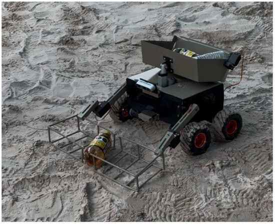
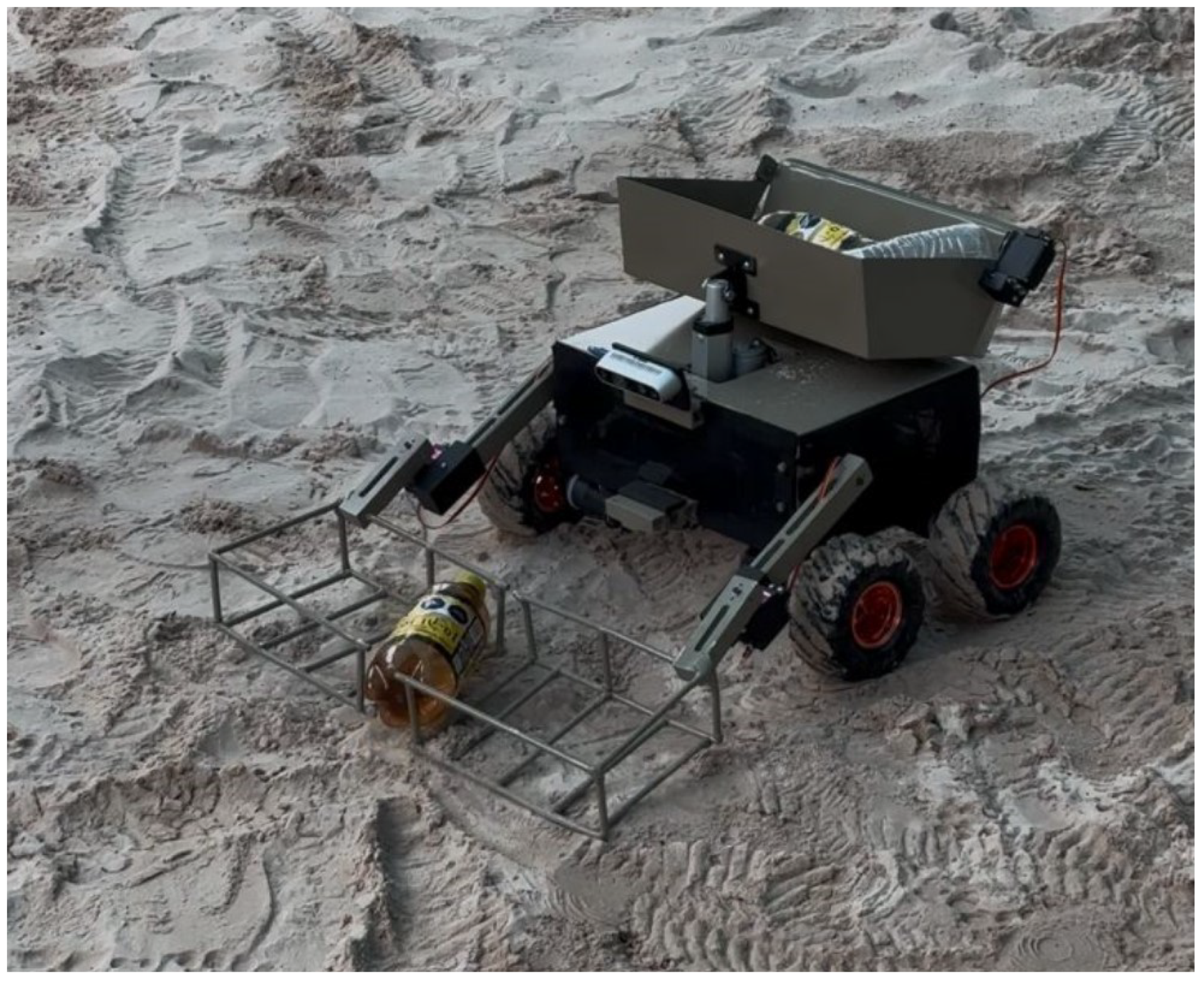
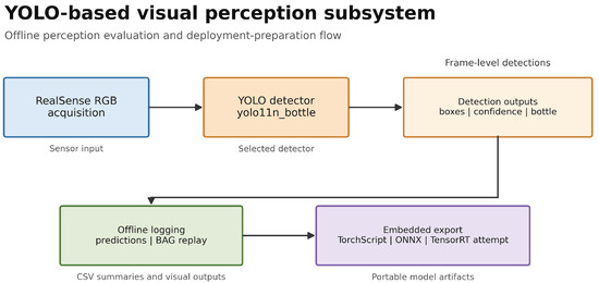
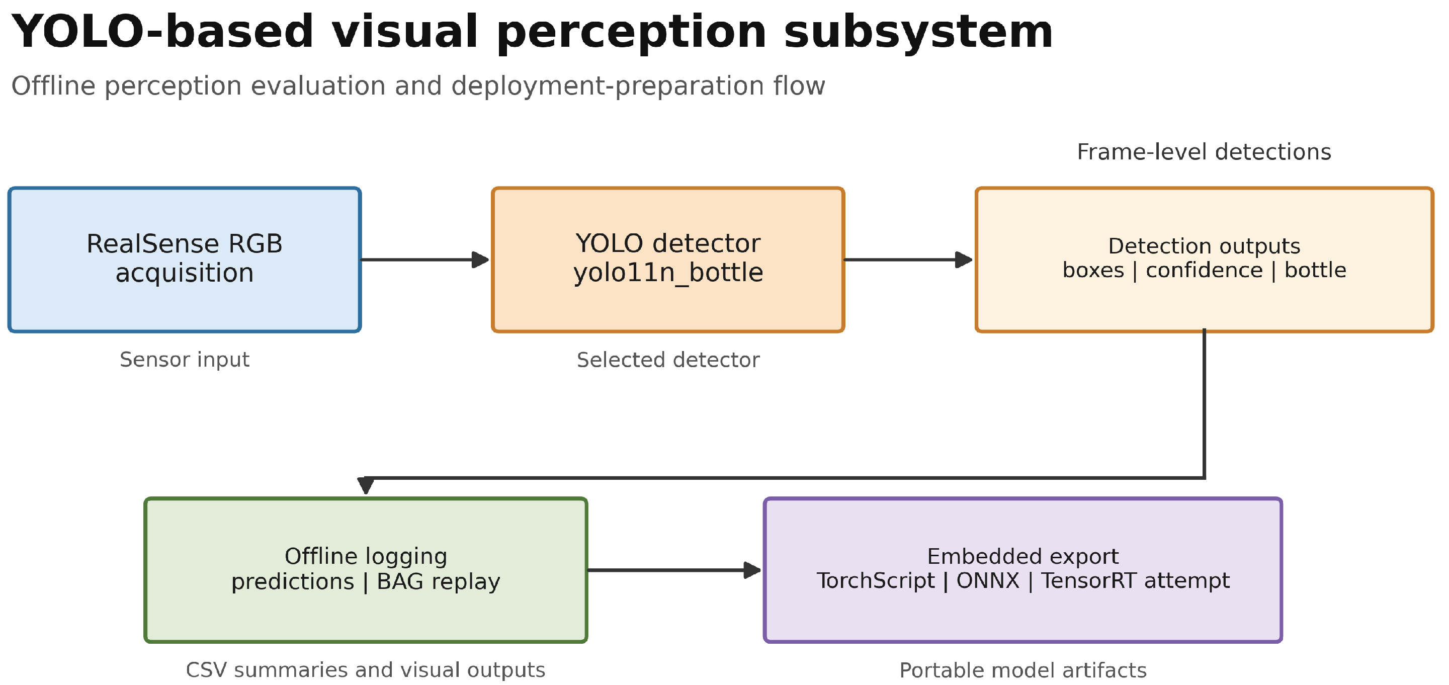


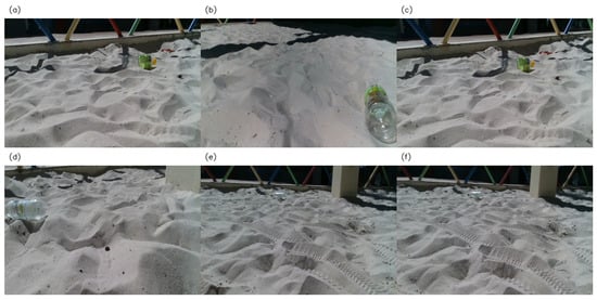
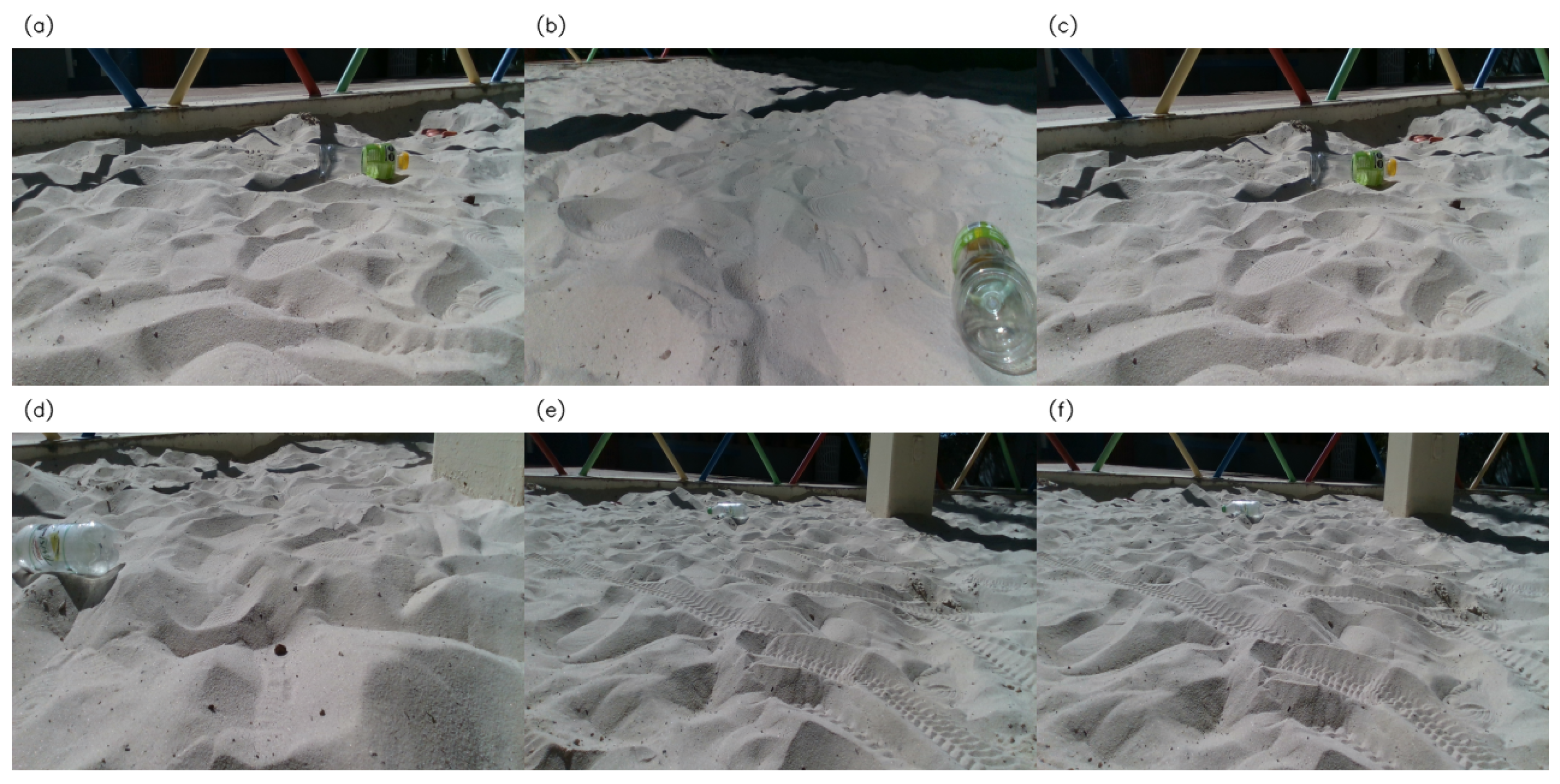
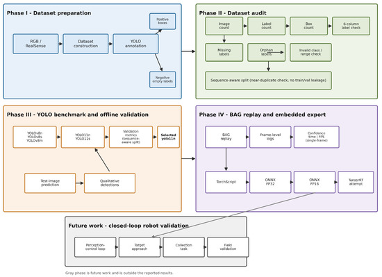
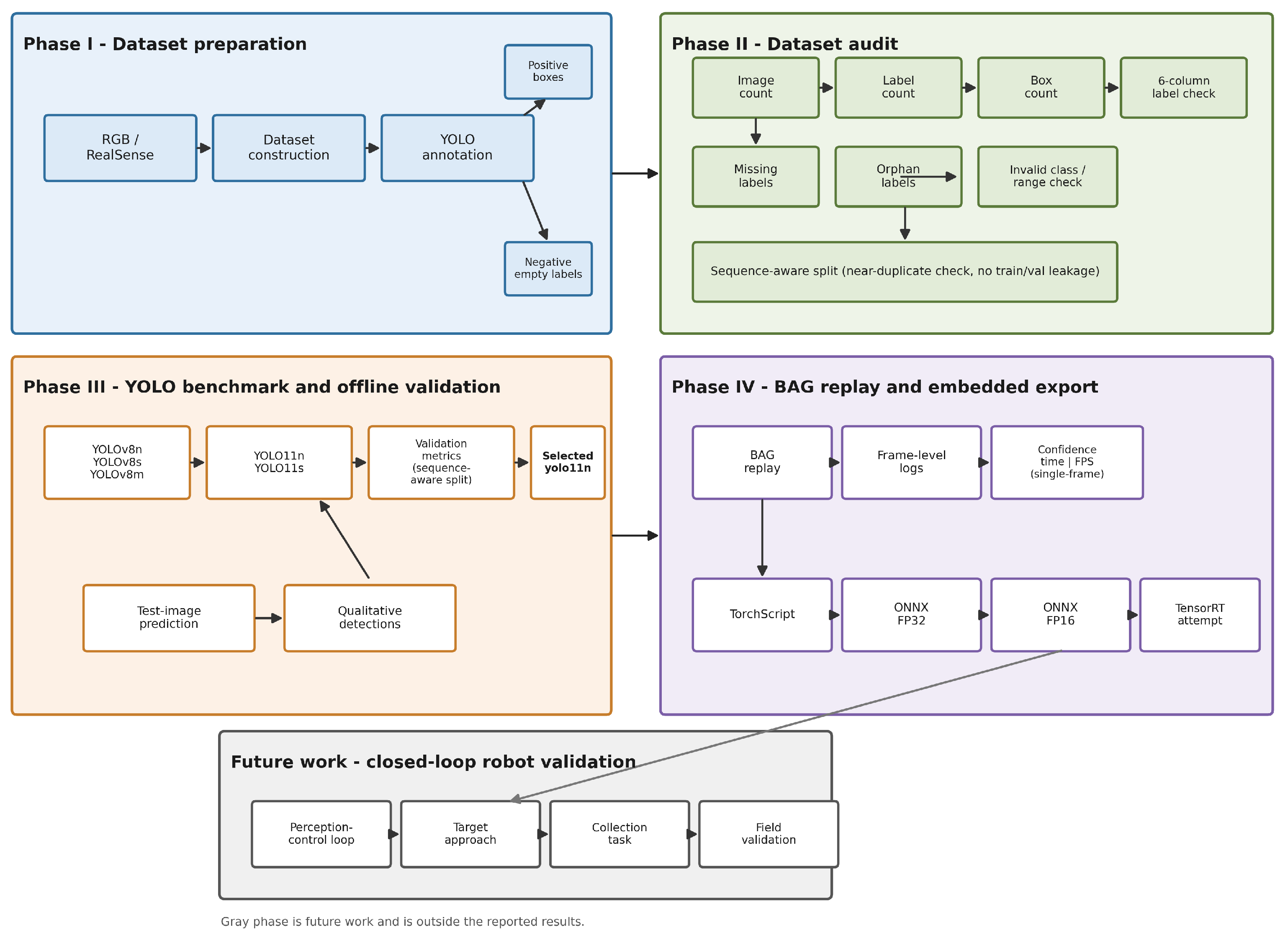


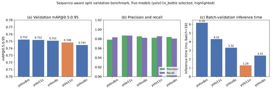
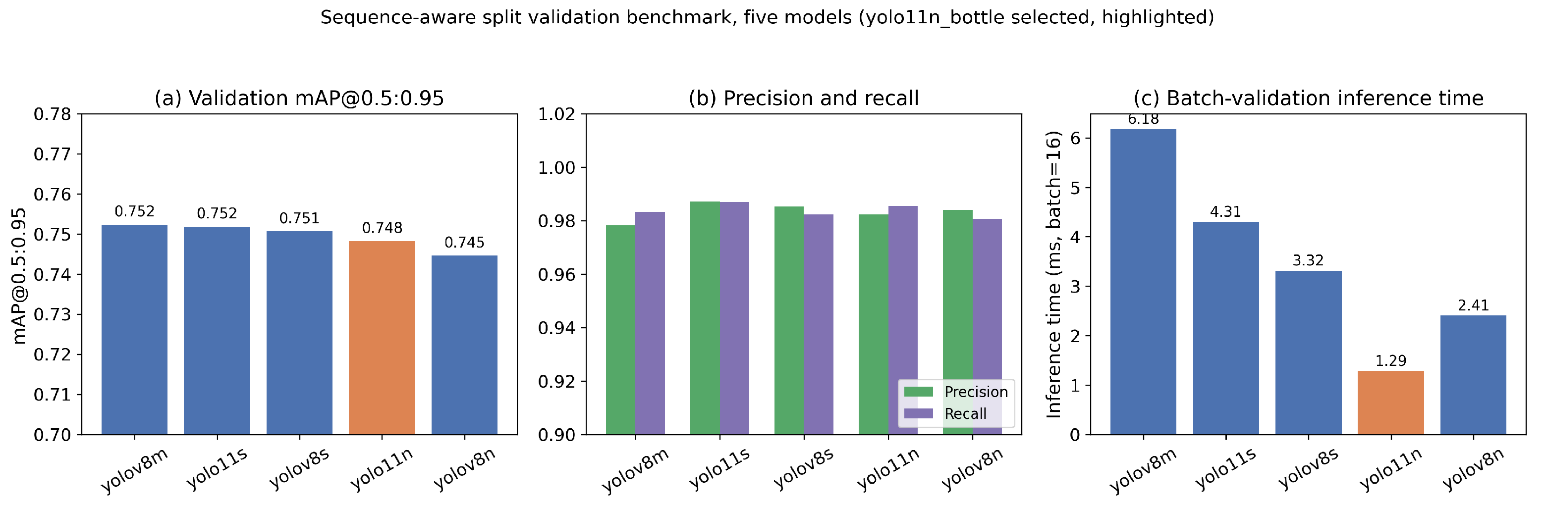
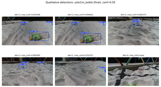
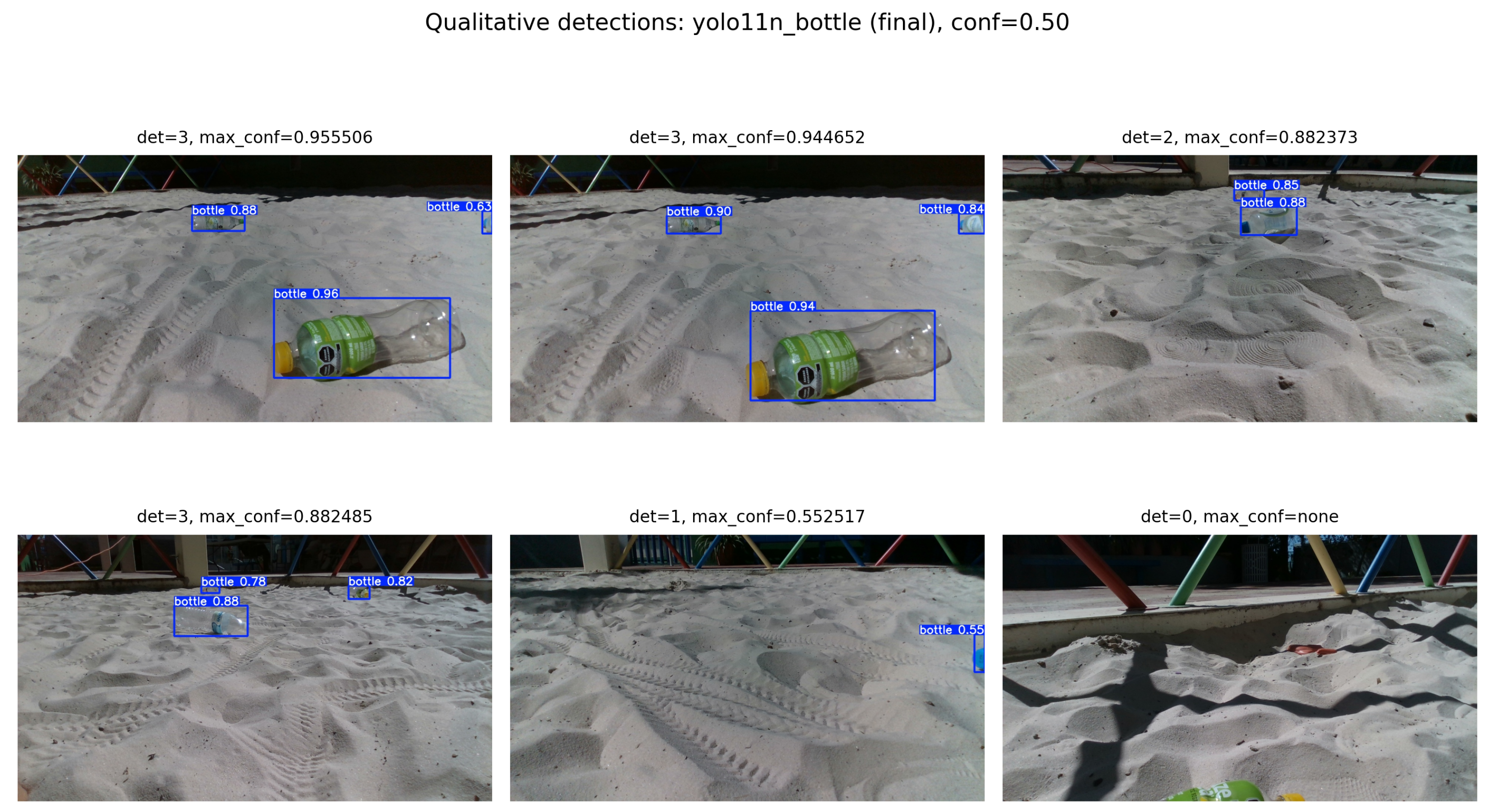
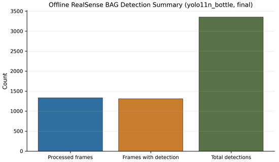
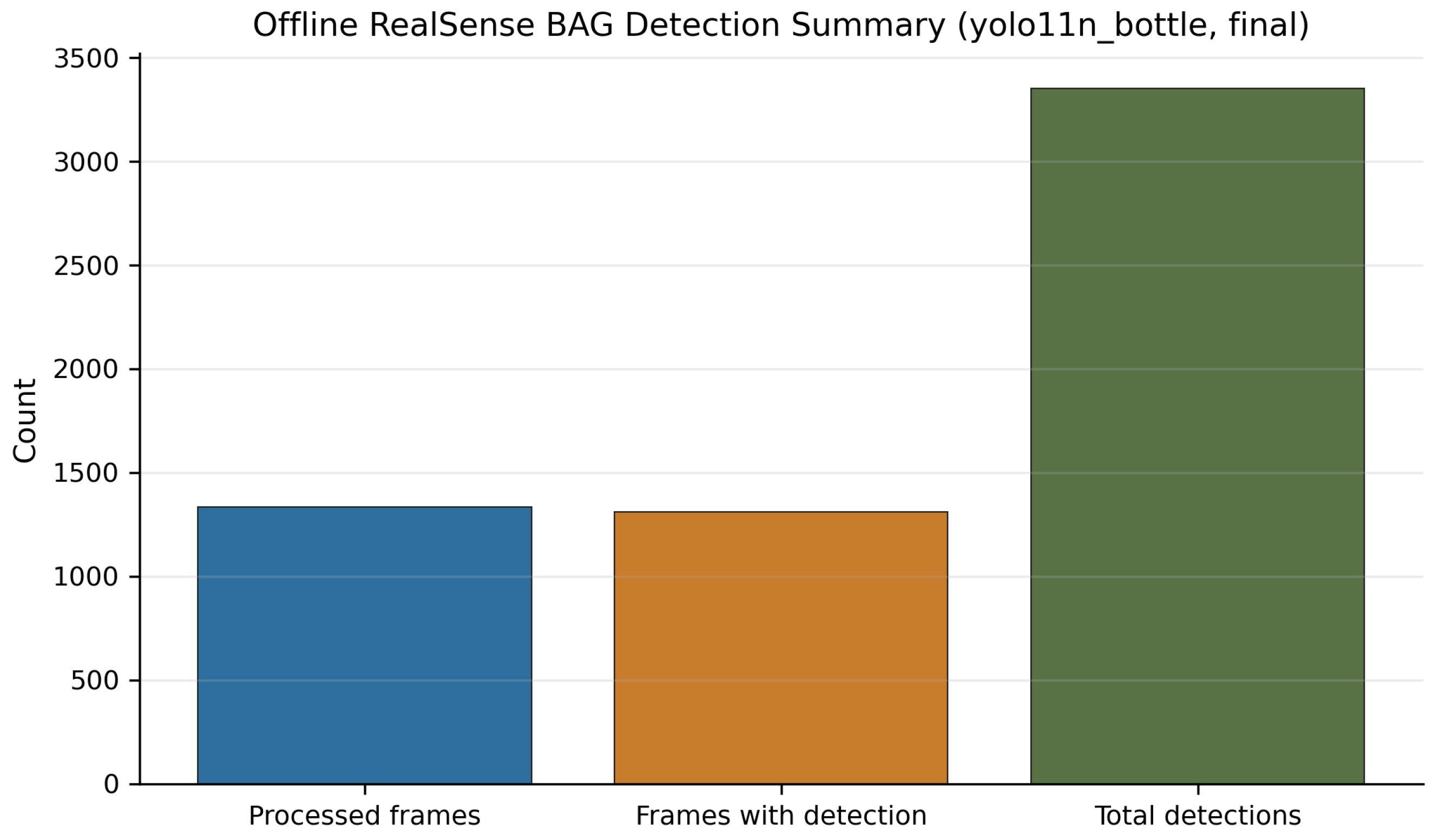
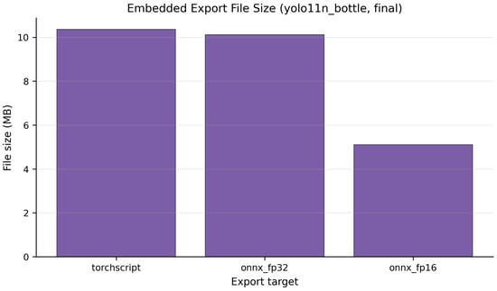
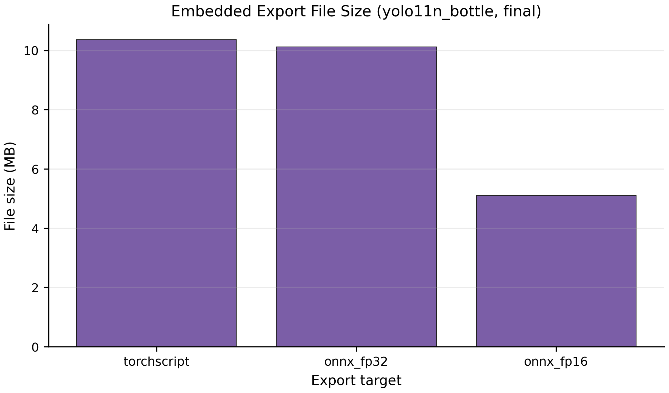

Disclaimer/Publisher’s Note: The statements, opinions and data contained in all publications are solely those of the individual author(s) and contributor(s) and not of MDPI and/or the editor(s). MDPI and/or the editor(s) disclaim responsibility for any injury to people or property resulting from any ideas, methods, instructions or products referred to in the content. |
© 2026 by the authors. Licensee MDPI, Basel, Switzerland. This article is an open access article distributed under the terms and conditions of the Creative Commons Attribution (CC BY) license.