


Abstract
Heart rate variability (HRV) forms the basis of non-invasive autonomic nervous system assessment. However, its analysis is constrained by the non-stationary nature of physiological signals. Standard analytical methods, which assume stationarity within fixed time windows, fail to capture dynamical effects of interest, such as the response to a physiological stressor. This limitation obstructs the development of mechanistic hypotheses about autonomic control. Here, we address this challenge by introducing a probabilistic framework for modeling non-stationary HRV dynamics during transient, single-event perturbation-recovery paradigms. We propose a hypothesis-driven, generative model that transforms the physiological response into a continuous-time stochastic process controlled by a double-logistic function. This approach deconstructs the R-R interval (RRi) series into a set of interpretable parameters representing the latency, rate, and magnitude of distinct response and recovery phases. Through simulation, we show that the model achieves high-fidelity parameter recovery and describes these dynamics more accurately than conventional fixed-time window methods under conditions matching its own generative assumptions. We then apply the framework to an empirical exercise-recovery recording, generating a precise, falsifiable hypothesis of “dissonant autonomic recovery”, where the baseline RR interval and its variability recover to distinct extents. The biphasic autonomic non-stationary decomposition (BAND) framework provides a formal methodology for translating RRi time series into quantitative, testable estimates of their generative processes.
1. Introduction
A major goal of contemporary biomedical science is to mechanistically connect the dynamic behavior of physiological systems to outcomes in human health and disease. The primary obstacle to this goal is the inferential gap between what can be measured with high temporal resolution via wearable sensors and the underlying neurobiological processes that generate these measurements [1]. This inverse problem is particularly evident in the study of the autonomic nervous system (ANS), where heart rate variability (HRV) has become the dominant non-invasive marker [2,3,4]. The R-R interval (RRi) time series is a highly informative signal, yet it presents a substantial analytical challenge, as it reflects the integrated and dynamic interplay of multiple regulatory systems [5]. Addressing this challenge requires formal methodologies capable of deconstructing the composite signal into quantitative, interpretable, and testable estimates of its underlying generative processes. The urgency of this task is highlighted by the central role of autonomic dysregulation in conditions ranging from cardiovascular diseases [6,7] to anxiety and post-traumatic stress [8,9,10], where precise characterization of system dynamics is essential for diagnosis and treatment.
The analytical tools most widely employed in this field remain poorly suited to the task, as the prevailing paradigm relies on calculating summary statistics within fixed temporal windows, thereby imposing a static and linear worldview on a system that is inherently dynamic and non-linear. These methods assume stationarity, an assumption routinely disrupted during physiological transitions of scientific or clinical interest [11,12]. As a result, they can produce misleading or uninterpretable outcomes. For example, by averaging across stress recovery, such methods conflate the initial sympathetic surge with the subsequent parasympathetic rebound, yielding a single opaque number that obscures the system’s adaptive capacity [11,12]. In this way, the unavoidable distortion of RRi signals under non-stationary conditions may mask critical differences between a resilient individual, characterized by rapid recovery, and a vulnerable one, marked by dampened recovery, thereby concealing an essential biomarker of pathology [13]. As a result, the “discretize-and-summarize” approach discards the temporal structure of the data and precludes direct estimation of core mechanistic properties such as response latencies, rates of change, and adaptive magnitudes, which represent the essential features that define the physiological process [14].
More sophisticated approaches have been proposed, but a substantial gap remains in methods that combine explicit non-stationary modeling with a structure suited to parameterizing discrete, transient physiological events. Time–frequency decompositions such as the wavelet transform provide detailed visualizations of spectral dynamics, making them valuable for exploratory analysis [15]. Yet they remain fundamentally descriptive, unable to instantiate a generative model of the underlying biology. These methods can demonstrate that a change has occurred, yet they are unable to provide a parameterized and testable explanation of the underlying nature of that change [16]. Modeling traditions like state-space models (SSMs) offer mathematical sophistication for tracking and forecasting system evolution [17,18]. While powerful, these models frequently sacrifice physiological fidelity for mathematical convenience, as their latent states are often defined by statistical rather than biological properties [18,19]. A further body of work, including point-process models of heartbeat timing and time-varying autoregressive (TVAR) spectral estimators, occupies an intermediate position: these approaches explicitly accommodate non-stationarity and, in some formulations, retain a link to physiological interpretation, but they are not typically structured to parameterize the discrete onset-and-recovery phases of a single, transient perturbation [20,21]. Even in these tailored applications, none of the above traditions are explicitly structured to parameterize the discrete phases of physiological events, such as onset rate, recovery latency, or adaptive magnitude in response to stress [18,19]. The field thus remains only partially served by these tools, which variously trade off non-stationary flexibility, physiological interpretability, and explicit event-level parameterization, rather than offering all three simultaneously.
Bridging this gap requires a conceptual shift from model-agnostic data description to the construction of hypothesis-driven frameworks grounded in generative modeling. Instead of simply characterizing what the data looks like, the focus should be on constructing explicit, testable, and quantitative models of the biological processes that generate the data. Here, we introduce and validate the biphasic autonomic non-stationary decomposition (BAND) framework, which reframes physiological analysis as a form of formal hypothesis testing. We hypothesize that autonomic responses to acute perturbations constitute structured, dynamic processes that can be effectively modeled as continuous-time stochastic process. Specifically, we employ a double-logistic function as a parsimonious hypothesis for biphasic dynamics, capturing the characteristic onset and recovery phases [22]. This representation translates raw signals into a small set of interpretable parameters, including the latency, rate, and magnitude of each phase, thereby providing direct insight into autonomic reactivity and resilience. This double-logistic formulation builds directly on our earlier work establishing its use for the time-domain trend of a single physiological signal [22]. The present framework extends that foundation in three specific ways: it jointly parameterizes the location (mean RRi) and dispersion (SDNN-scale) trajectories under a shared timing structure, enabling direct, quantitative contrasts between their recovery extents; it embeds a full spectral decomposition, partitioning structured variance across physiological frequency bands via Gaussian-process oscillators; and it unifies both the time-domain and frequency-domain components within a single, jointly estimated Bayesian model with complete posterior uncertainty quantification, rather than treating trend estimation as a standalone curve-fitting exercise.
2. Results
We propose a framework based on a generative Bayesian model that yields robust parameter estimates with full uncertainty quantification and, owing to its Bayesian formulation, is naturally extensible to hierarchical inference across individuals and groups in future work. The model decomposes the RRi series into a time-varying mean, total variance, and a dynamically shifting oscillatory component controlled by a double-logistic latent dynamic. Under conditions matching the model’s own generative assumptions, this formulation provides a more accurate and physiologically interpretable representation of autonomic dynamics than conventional fixed-window methods, offering quantitative indices of reactivity and recovery and a principled means to translate complex time series into mechanistic, falsifiable hypotheses.
After its construction, we test the BAND model’s internal consistency by assessing its ability to recover its own parameters from simulated data. We then benchmark its descriptive fidelity against conventional methods to quantify its effectiveness in characterizing dynamic signals. Finally, we use the framework to generate a structured, phenomenological description of an empirical exercise-response signal, illustrating its potential for developing precise and data-driven hypotheses.
The core components of the model and their relation to the underlying data generation process being modeled are illustrated in Figure 1.
Figure 1.
Core inferential procedure being captured by the model. The data generation process being modeled is a transient stressor or perturbation from a baseline to a recovered state (1). This stimulus is being applied while the R-R intervals (RRis) are being recorded simultaneously (2). Then, the biphasic autonomic non-stationary decomposition (BAND) model takes the RRi data and decomposes the data generation process as a linear combination of time and frequency components that build the underlying observed RRi signal as a dynamical and continuous process (3).
2.1. Model Validation and Parameter Recovery on Synthetic Data
To establish the model’s internal consistency and the identifiability of its parameters, we first assessed its ability to perform inference on synthetic data generated from its own structure. This in silico procedure serves as a necessary check of the model’s self-consistency and the estimation algorithm’s ability to navigate the complex posterior geometry. To test the model’s performance, three distinct scenarios were designed: (A) a canonical response with complete recovery; (B) an incomplete recovery with persistence in both time and frequency domains; and (C) a high-noise condition with a low structured variance fraction ( = 0.6). The ground-truth dynamics are illustrated in Figure 2, with corresponding generative parameter values listed in Table 1. This procedure tests for inferential integrity under the assumption that the model is correctly specified; it does not test for robustness to model misspecification, a challenge inherent to all empirical data.
Figure 2.
Ground-truth dynamics of three synthetic scenarios. The scenarios were designed to test model performance under diverse conditions: (A) a classic sympatho-vagal response, (B) an incomplete recovery with persistence in both time and frequency domains, and (C) a high-noise condition with dissonant (complete time-domain, incomplete spectral) recovery. Panels show the generated RRi data with the true mean signal, the underlying time-domain trajectories for baseline RRi and total SDNN, and the time-varying spectral proportions.
When fit to this synthetic data, the model demonstrated a high-fidelity reconstruction of the generative process across all three scenarios. Figure 3 presents a visual summary of these results, plotting the model’s posterior estimates against the known ground-truth trajectories. The posterior means for the baseline RRi, total SDNN, and the time-varying spectral proportions closely track the true underlying dynamics. The 95% credible intervals, which represent the range of plausible parameter values given the data, consistently envelop the ground-truth trajectories.
Figure 3.
High-fidelity reconstruction of synthetic data by the generative model. The model’s posterior mean estimates (solid lines) and 95% credible intervals (shaded ribbons) are overlaid on the known ground-truth dynamics (dashed lines) for all three scenarios (A–C). The model accurately recovers the continuous trajectories for baseline RRi, total SDNN, and spectral proportions across all conditions.
Table 1.
Ground-truth parameter values for simulation scenarios. Ground-truth parameter values used in the generation of three simulation scenarios. The scenarios correspond to (A) a classic sympatho-vagal response, (B) an incomplete recovery with time-domain and spectral persistence, and (C) an incomplete spectral but complete time-domain recovery with high noise.
Beyond recovering the continuous dynamic trajectories, the model also recovered the discrete parameters that govern the shape and timing of these dynamics. Table 2, Table 3 and Table 4 present the posterior summaries for these key parameters, comparing the posterior median and 95% credible intervals against their true values. For all parameters across all scenarios, the 95% credible intervals successfully contained the ground-truth values. This three-scenario test serves as a proof-of-concept parameter-recovery demonstration, rather than a general claim of practical identifiability; a more systematic characterization, including simulation-based calibration across a broader range of data configurations, is reported below and in the Supplementary Materials.
Table 2.
Posterior recovery of ground-truth parameters—Scenario A (classic sympatho-vagal response). This table compares the known ground-truth parameter values to the model’s posterior estimates (median and 95% credible interval) for Scenario A. The model successfully recovers all parameters, with the true values consistently falling within the credible intervals.
Table 3.
Posterior recovery of ground-truth parameters—Scenario B (incomplete recovery with time-domain and spectral persistence). This table compares the known ground-truth parameter values to the model’s posterior estimates (median and 95% credible interval) for Scenario B. The model successfully recovers all parameters, with the true values consistently falling within the credible intervals.
Table 4.
Posterior recovery of ground-truth parameters—Scenario C (incomplete spectral, complete time-domain recovery, high noise). This table compares the known ground-truth parameter values to the model’s posterior estimates (median and 95% credible interval) for Scenario C. The model successfully recovers all parameters, with the true values consistently falling within the credible intervals.
Benchmarking the Model’s Descriptive Fidelity
Having established the model’s internal consistency, we next benchmarked its descriptive performance against conventional, widely adopted analytical methods. The objective of this comparison was to quantify the core differences in how these analytical frameworks represent and summarize dynamic signals and to highlight the specific conditions under which our proposed model offers a more advantageous description and performance. The same synthetic datasets from the previous section were analyzed using a 60-s sliding-window analysis for time-domain metrics (mean RRi and SDNN) and a Short-Time Fourier Transform (STFT) with a similar window length for characterizing spectral dynamics. The STFT, and similar Fourier methods, allow the decomposition of the signal into frequency bands that compose the complete signal, which helps in the identification of the relative contribution of major frequency bands (which the BAND model mechanistically performs as part of its architecture). As an additional and more robust comparator for spectral reconstruction, we also benchmarked the model against a Continuous Wavelet Transform (CWT) analysis, given that this method does not impose the fixed time–frequency resolution trade-off inherent to sliding-window and STFT-based approaches [15].
The results of this comparative analysis highlight the descriptive distortions that are inherent to any method that relies on assumptions of local stationarity when applied to a continuously varying, non-stationary signal. Figure 4 illustrates the outputs from the windowed methods (the CWT method performance is shown separately in Supplementary Figure S11). Visually, these methods produced a delayed and morphologically blunted approximation of the underlying dynamics. The sharp, non-linear transitions that characterize the onset and recovery phases of the signal are smeared and flattened by the averaging process inherent in the windowed calculation. Consequently, the windowed approach failed to accurately capture both the shape and the precise timing of the recovery process. Instead of reflecting the smooth, logistic curve defined by the ground-truth process, the windowed analysis superimposed the square-wave artifacts of its own computational structure onto the data, a clear instance of the analytical method distorting the phenomenon it is intended to measure.
Figure 4.
Distorted reconstruction of synthetic data by conventional windowed methods. The estimates from a 60-s sliding window (for RRi and SDNN) and an STFT (for spectral proportions) are shown as solid lines overlaid on the ground-truth dynamics (dashed lines). The methods introduce significant lag, blunting, and temporal smearing, failing to capture the true non-linear dynamics. First upper row shows the mean R-R reconstruction, middle row shows time-dependent scale and bottom row shows spectral proportion reconstruction. The three presented scenarios were designed to test model performance under diverse conditions: (A) a classic sympatho-vagal response, (B) an incomplete recovery with persistence in both time and frequency domains, and (C) a high-noise condition with dissonant (complete time-domain, incomplete spec-tral) recovery.
A formal quantitative analysis confirms the descriptive efficiency and accuracy of the generative approach for signals of this particular nature. Table 5 and Table 6 provides a summary of key performance metrics for windowed and wavelet-based methods (Table 5) and BAND framework (Table 6). Across all scenarios and all signal components, the generative model consistently provided a more accurate and parsimonious description of the data. It achieved substantially lower error (RMSE and Bias) and captured a significantly higher proportion of the signal’s variance, with values typically exceeding 0.90. It is important to interpret this result with caution. The model’s performance is, in one sense, expected, as the synthetic data were generated from its own structure. However, it illustrates a core theoretical argument of this work: for signals that are plausibly characterized by smooth, continuous transitions between distinct physiological states, a model whose parametric form explicitly encodes this structure will naturally provide a more efficient, less distorted, and more interpretable quantitative summary than a non-parametric, windowed approach that was designed for stationary or quasi-stationary signals.
Further model diagnostics testing the model’s overall stability and reliability on synthetic data for in silico validation can be found in the Supplementary Materials. Prior predictive checks are shown in Figure S1, prior sensitivity analysis in Figure S2, full posterior distributions in Figure S3, and model fit to asymmetric recovery data from a different data generation process in Figure S4. Additionally, non-Gaussian distributions are presented in Figure S5. Beyond these three fixed scenarios, we also report a pairwise posterior-correlation analysis for , , , and , and replicate the asymmetric-recovery and non-Gaussian misspecification checks quantitatively across repeated simulation runs rather than as single visual examples. We further strengthened the residual diagnostics for all misspecification checks to include autocorrelation, conditional-variance, and tail-behavior assessments, rather than global mean/SD recovery alone. Consistent with the model’s stated scope as a single-event instrument (Section 3.3), we did not extend these checks to multiple or overlapping perturbations.
Table 5.
Quantitative performance metrics for the sliding-window (SW) and wavelet-based (CWT) methods across simulated conditions (A, B and C). This table presents the root mean squared error (RMSE) and mean absolute error (MAE), reported in milliseconds for RRi and SDNN-scale metrics, as a dimensionless proportion for spectral (implied variance-share, ) metrics, as measures of the average magnitude of the estimation error, as bias (mean error, same units) to identify any systematic tendency for over- or underestimation, and as the coefficient of determination (, dimensionless) to assess the proportion of variance in the true signal captured by the estimate. Intervals reported for the SW and CWT comparators are 95% bootstrap intervals obtained by resampling the underlying synthetic record, so that all methods are reported with comparable uncertainty quantification. Decimal precision is unified to three significant figures throughout.
Table 6.
Quantitative performance metrics for the generative model across simulated conditions (A, B and C). This table presents the root mean squared error (RMSE) and mean absolute error (MAE) and SDNN-scale metrics as a dimensionless proportion for spectral (implied variance-share, ) metrics and as measures of the average magnitude of the estimation error, as bias (mean error, same units) to identify any systematic tendency for over- or underestimation, and as the coefficient of determination (, dimensionless) to assess the proportion of variance in the true signal captured by the estimate. Intervals reported for the generative model are 95% posterior credible intervals computed across MCMC draws.
2.2. A Phenomenological Description of an Empirical Exercise Response
To illustrate the framework’s intended application in a real-world context, we analyzed an RRi time series recorded from a single healthy subject undergoing a standardized two-minute submaximal step test. The express purpose of this N-of-1 analysis is to demonstrate how the model translates a complex, high-dimensional, and noisy time series into a concise, low-dimensional, and interpretable set of parameters that form the basis for generating new, quantitative, and ultimately falsifiable hypotheses.
Upon fitting the model to the empirical data, it yields a phenomenological decomposition of the entire exercise-recovery response, as depicted in Figure 5. The framework parses the signal into its constituent components, describing the physiological process as a rapid initial tachycardia (a decrease in the baseline RRi component, panel A and B in Figure 5) and a concurrent suppression of total heart rate variability (a decrease in the SDNN component, panel C in Figure 5). This initial response is followed by a slower, more gradual recovery phase after the cessation of the exercise stimulus. From a spectral perspective, the model attributes the signature of this response to a near-complete withdrawal of power in the high-frequency (HF) band and a corresponding surge in the proportion of very-low-frequency (VLF) power (panel D in Figure 5). The model captures these dynamics as continuous, smooth trajectories, providing an integrated narrative of the entire physiological event.
Figure 5.
Phenomenological decomposition of an empirical exercise-recovery response. The figure illustrates the reconstructed RRi signal (red line in panel A) overlaid on top of the observed RRi signal (gray). In the bottom panel, the biphasic autonomic non-stationary decomposition (BAND) model components appear. First, the time-domain components: the baseline RRi trend (, blue line, panel B) and the total instantaneous variability (, SDNN-scale, orange, panel C). Additionally, the inferred dynamics of the spectral mixture weights, , is also present, describing the evolution of frequency band relative participation across the transient stimulus (panel D). The shaded regions represent the 95% highest density intervals.
The framework’s primary scientific utility, however, lies in generating quantitative, testable claims, which are encapsulated by the posterior distributions of its parameters. A key feature of the model is its separate parameterization of the recovery dynamics of the signal’s location (mean RRi, via the coefficient ) and its dispersion (total variability, or SDNN-scale, via the coefficient ). Because both trajectories share the same underlying timing parameters (, , , ; Equation (6)), and do not describe a difference in recovery rate or timescale; rather, they quantify a difference in recovery extent, the asymptotic fraction of the initial perturbation that is undone. This explicit separation allows for a direct, quantitative description of their potential divergence in extent. In this particular recording, the posterior distributions for these two recovery-extent parameters were credibly distinct; the 95% credible interval for (median of the posterior distribution = 0.69, CI95%[0.66, 0.73]) was clearly separated from that for (median = 1.05, CI95%[0.94, 1.16]). This descriptive feature of the model’s output, which we term model-inferred dissonance, provides a data-driven and falsifiable hypothesis: that the baseline RR interval and its variability can recover to distinct and dissociable extents in response to an acute exercise stressor. This hypothesis is a quantitative statement, grounded in the posterior probability distributions of the model’s parameters.
Empirical and visual model diagnostics can be seen in the Supplementary Materials. Complete traceplots, posterior distributions and MCMC diagnostics can be seen in Figure S6 and Figure S7 and Table S3, respectively. Posterior and distributional predictive checks can be seen in Figures S8 and S9.
3. Discussion
The quantitative analysis of HRV has long been a primary method for the non-invasive study of the autonomic nervous system [2,23]. A persistent challenge in this field is the inherent non-stationarity of physiological signals, which directly conflicts with the foundational assumptions of traditional analytical techniques [11,12,24], which were often adopted due to the computational constraints of their era. This discrepancy necessitates the use of methodological compromises, most notably time-windowing, which can introduce significant analytical artifacts and obscure the very dynamics they seek to quantify [13,25]. The present study was undertaken to develop and evaluate a generative probabilistic model for RRi time series, explicitly designed to represent and infer the parameters of transient physiological events. Our findings, based on a comprehensive suite of simulations and an empirical application, suggest that the BAND framework offers a more accurate and granular characterization of autonomic dynamics compared to what conventional windowed approaches can achieve. Our generative model provides a more detailed characterization of autonomic dynamics; however, its interpretation requires careful consideration of its underlying assumptions.
The primary contribution of this research is the synthesis and application of established Bayesian inference principles to construct a purpose-built, physiologically oriented measurement instrument [26]. The model formalizes a specific, falsifiable hypothesis about the data-generating process underlying dynamic RRi signals. We employ the term generative in its formal statistical sense: the model specifies a complete joint probability distribution over both parameters and observed data, such that synthetic RRi series can, in principle, be simulated forward from any given parameter set, and Bayesian inference can be run in reverse to recover a posterior distribution over those parameters given observed data. This usage should be clearly distinguished from a mechanistic or biophysical generative model of the underlying physiology. BAND does not simulate the coupled dynamics of vagal efferent activity, sympathetic outflow, baroreflex gain, or sinoatrial node pacemaker kinetics; it generates the statistical shape of the RRi signal, not the biological processes that produce it. The double-logistic and spectral-oscillator components should therefore be understood as a flexible, phenomenological description of how the signal’s mean and variance evolve, chosen for its mathematical tractability and interpretability, rather than as a reduced-form representation of any specific physiological circuit. The internal validity and statistical integrity of this inferential process were examined through extensive simulation studies. In these controlled in silico experiments, where the ground truth was known, the model consistently recovered the generative parameters, and its posterior credible intervals were well-calibrated [27,28]. The model’s successful parameter recovery in these controlled simulations provides baseline confidence in its function as a reliable measurement device, but only under conditions where its numerous and restrictive structural assumptions are perfectly met. When benchmarked against conventional methods under conditions matching its own generative assumptions, more accurate performance in tracking dynamic signals was observed. This is an expected consequence of its design, which replaces the crude filtering of windowing with a formal, continuous model of the underlying process. However, the apparent sophistication of this approach belies a series of deep-seated assumptions and conceptual challenges that demand scrupulous consideration.
3.1. Methodological Trade-Offs and the Abandonment of Stationarity
A core assertion of this work is that the analytical shortcomings of traditional HRV analysis are conceptual, not merely technical. Windowed methods are, in essence, digital filters [29]. As such, they inevitably distort the signal they are intended to measure, introducing lag, attenuating amplitudes, and enforcing a false dichotomy between temporal and spectral resolution as dictated by the Heisenberg-Gabor uncertainty principle [30]. The inferential approach adopted here avoids these specific artifacts by modeling the entire time-course of an event holistically. Information from every data point is leveraged to inform the estimate at every other data point, conditioned on the assumed model structure [31].
However, this approach introduces its own set of abstractions. A potentially problematic assumption is the model’s imposition of orthogonality on a non-orthogonal system. The model specifies the observed RRi signal as a linear, additive combination of a baseline trend, several sinusoidal components, and a residual noise term. This mathematical decomposition is elegant and ensures parameter identifiability [32,33]; nonetheless, it is a convenient simplification of cardiovascular physiology.
Similarly, in physiology, the systems underlying these model components are deeply and non-linearly coupled. Baroreflex activity (a major contributor to the low-frequency component) and respiratory sinus arrhythmia (the high-frequency component) are not independent processes that sum together; they are neurologically intertwined within the brainstem and are engaged in a constant, dynamic feedback loop [34,35]. By construction, the model is designed to assign variance to its clean, orthogonal components in a way that may not map cleanly onto the underlying biology. The estimate for the amplitude of the high-frequency component, for instance, should be interpreted as the magnitude of the best-fitting sinusoidal component in that band, assuming it can be linearly and additively separated from all other ongoing dynamics, rather than a pure measure of respiratory sinus arrhythmia. The model’s simplifying assumption of linear, additive separation is an important caveat for physiological interpretation that requires careful consideration [36].
This caveat extends to the standard physiological labels conventionally attached to each frequency band, and we state them explicitly here because they apply throughout this manuscript wherever spectral band proportions are discussed, including the empirical case study in Section 2.2. High-frequency (HF) power is often equated with parasympathetic (vagal) activity, but this equivalence is only secure when respiratory rate and depth are also measured and shown to remain within the canonical HF band; without concurrent respiratory monitoring, HF amplitude should be treated as an index of oscillatory power in that frequency range, not a validated measure of vagal tone [37]. Low-frequency (LF) power is even less specific: it reflects a mixture of sympathetic, parasympathetic, and baroreflex-mediated influences rather than sympathetic activity alone, and the once-common LF/HF ratio as a marker of “sympathovagal balance” is not supported by current evidence [37]. Very-low-frequency (VLF) power is the least well characterized physiologically, and its estimation from short, single-event recordings of the kind analyzed here carries particularly limited interpretability, given the small number of complete VLF cycles such records typically contain [37].
3.2. From Statistical Constructs to Biological Reality
The intended value of this framework is its ability to distill a complex signal into a set of “interpretable” parameters. This claimed interpretability, however, occupies a position between useful abstraction and the risk of equating a parameter with a physical process [38,39]. The very act of assigning a label like “recovery rate” to a parameter () cognitively biases the researcher to perceive it as a distinct, tangible biological process [40]. While the parameter perfectly describes a feature of the fitted mathematical curve, it is an unsubstantiated inferential leap to equate it with a singular neurophysiological mechanism [39,41]. The observed recovery trajectory is the net result of an immensely complex cascade of interacting neural, endocrine, and humoral processes [13,35,42]. The model’s parameterization of this trajectory is a descriptive summary, rather than an elucidation of its constituent parts.
Such interpretive discipline, separating a mathematical parameter from a singular biological process, must be applied to all model outputs. The concept of “dissonant autonomic recovery”, for example, is a statistically identifiable pattern where the baseline RR interval recovers to its resting value far more quickly than measures of heart rate variability recover to theirs [43]. Yet, its proposed link to “lingering sympathetic activation” remains a speculative hypothesis requiring external validation. Could this pattern alternatively reflect differential downregulation rates of adrenergic and cholinergic receptors, or a mismatch in the resetting of central autonomic command versus peripheral feedback? These are precisely the kinds of hypotheses the model allows one to formulate, but it possesses no inherent capacity to adjudicate between them. It provides the tool to quantify the phenomenon with precision, thereby allowing for the examination of such hypotheses [44], but it cannot, on its own, provide definitive causal evidence.
This proposed dissociation is not without physiological precedent, and situating it against known autonomic kinetics helps clarify why it is a plausible hypothesis rather than an ad hoc pattern. The two branches of the autonomic nervous system act on markedly different timescales: parasympathetic (vagal) influence on the sinoatrial node is mediated by acetylcholine acting through fast-activating potassium channels and is rapidly terminated by local acetylcholinesterase activity, producing beat-to-beat changes in heart period within a few cardiac cycles [45,46]. Sympathetic influence, by contrast, is mediated by norepinephrine acting through slower second-messenger cascades and is cleared more gradually through reuptake and diffusion, so its effects unfold over tens of seconds to minutes [45,46]. If the comparatively fast recovery of mean RRi observed here reflects predominantly vagal reactivation, while the slower recovery of total variability reflects a more gradual sympathovagal rebalancing, a dissonant pattern of this kind is broadly consistent with these established differences in autonomic kinetics.
A related candidate mechanism is post-exercise baroreflex resetting. Baroreflex sensitivity is transiently blunted following acute exercise and returns to baseline on its own, comparatively slow timescale, which need not coincide with the return of heart rate to resting values [34,35]. Because baroreflex-mediated buffering contributes substantially to the oscillatory, rhythmic component of RRi variability that the model’s spectral decomposition targets, a lag between baroreflex recovery and heart-period recovery offers a second, non-mutually exclusive physiological candidate for the pattern the model detects. Consistent with the interpretive caution urged throughout this section, we emphasize that the present analysis cannot adjudicate between these or other specific mechanisms; its purpose is to establish that the dissonance hypothesis is grounded in established autonomic physiology rather than a statistical artifact and that it therefore merits the kind of targeted, mechanism-isolating follow-up (e.g., pharmacological blockade studies) proposed in Section 3.4.
Nowhere is this interpretive caution more warranted than with the structured variance fraction, . At its core, is simply the proportion of signal variance captured by a fixed set of sinusoids, and it should be described in no more specific terms than that. A reduction in could plausibly reflect a pathological dysregulation of autonomic rhythms [47]. However, it could equally reflect a plethora of other confounders: an increase in movement artifact, the presence of uncorrected ectopic beats, a change in breathing frequency outside the canonical high-frequency band, or activation of other physiological processes that contribute to RRi variance but are not sinusoidal [12,13,14]. Labeling this or any other model parameter with a specific physiological construct is, at best, premature and risks imbuing it with a degree of certainty that it does not currently warrant.
3.3. Limitations
The model’s architecture is built upon a series of rigid assumptions. The choice of a symmetric double-logistic function is primarily mathematical [22], not a physiological imperative. Many biological recovery processes exhibiting asymmetry, hysteresis, or multi-timescale recovery would be poorly approximated by this functional form. Moreover, the model is a specialist instrument designed for a single, isolated perturbation-recovery event [22]. This makes it highly effective for analyzing clean, stimulus-response experimental paradigms but makes it unsuited for the exploratory analysis of complex, naturalistic data containing multiple, overlapping events of unknown form [12,24]. It is a tool for confirmatory, not exploratory science.
Furthermore, we acknowledge that the empirical validation of this framework is presently confined to a single-subject case study. This was a deliberate choice reflecting the manuscript’s primary aim: to introduce and validate a new methodological framework, not to make a generalizable empirical claim. The N-of-1 analysis serves as a proof-of-concept analysis, demonstrating the model’s ability to perform a deep phenotyping of an individual’s response and, most importantly, to generate precise, falsifiable hypotheses. We contend that establishing this hypothesis-generating capacity is a necessary prerequisite to the much larger, and computationally demanding, task of applying the model hierarchically to a full cohort. This foundational work is offered to empower the broader research community to test these newly generated hypotheses on larger, more diverse datasets.
The adoption of a Bayesian framework, while providing intuitive probabilistic outputs, comes with its own methodological assumptions. The posterior credible interval for a parameter is a statement of subjective belief about its value, conditional on the data, the chosen model structure, and the specified prior distributions [26]. It is not equivalent to a frequentist confidence interval and does not account for structural uncertainty, the possibility that the model itself is misspecified. This leads to what might be termed the “Rashomon effect” in modeling, where multiple, structurally different models can provide equally good fits to the data while telling different and contradictory stories about the underlying process [48]. Without a systematic exploration of this “model space”, the conclusions drawn from this single model must be regarded as highly provisional.
The model’s reliance on Hamiltonian Monte Carlo sampling makes it computationally expensive. The required runtime may not only be a practical barrier for large datasets but could also create an “analytical divide”, where such advanced methods are only accessible to research groups with substantial computational resources. This effectively sidelines the method from deployment in real-time or near-real-time clinical settings, such as intensive care monitoring, where rapid feedback is paramount. Furthermore, the model’s performance is closely tied to the fidelity of upstream data. Uncorrected premature ventricular contractions or excessive measurement noise, for instance, could drastically alter the local mean and variance of model parameters. While the model may be robust to small deviations, its behavior in the face of such gross, non-stationary artifacts is unknown and could lead to biased inference on the entire stress-recovery curve. Finally, the treatment of the residual term as unstructured “noise” is a convenient assumption. In biology, true randomness is rare; the residuals likely contain unmodeled, structured biological processes or deterministic chaos.
3.4. Future Directions
The limitations catalogued above define a necessary line for future research. This line of research should move beyond incremental model refinement and toward the systematic characterization of the model as a scientific instrument.
The most urgent task is to initiate the calibration process for this instrument. Just as a new telescope must have its optical aberrations mapped and its resolution quantified, this model requires a comprehensive characterization of its operational properties. An ideal future study would involve establishing a formal calibration protocol, creating a standardized open-source library of synthetic RRi signals with known complexities, asymmetric responses, overlapping events, various artifact types, and non-Gaussian noise, and then systematically testing the model against this library, following the precedent set by open physiological-signal repositories such as PhysioNet [49]. The results, published as a detailed “specification sheet”, would delineate the model’s biases, sensitivities, and failure modes, defining its safe operating envelope for future users.
Furthermore, future work should focus on utilizing the model for quantitative hypothesis testing and falsification. The framework should be applied in experimental contexts where specific interventions are known to target certain physiological pathways. For instance, testing the effect of beta-blockade on the response amplitude and recovery rate parameters following a cold pressor or exercise-based test would provide crucial external validation, linking the model’s abstract parameters to tangible pharmacological effects. This shifts the focus from “fitting a model” to “using a model to test a theory” [44,48].
The generative framework presented here represents a conceptually powerful alternative to conventional methods for analyzing dynamic HRV. Ultimately, this model should be viewed as a specialized instrument, rather than as a perfect reflection of reality. Its value lies in its ability to translate a complex signal into a set of precise, falsifiable hypotheses. The difficult work of calibrating this instrument, understanding its distortions, and cautiously deploying it to test concrete physiological hypotheses will ultimately determine its lasting contribution to the science of autonomic control.
4. Material and Methods
4.1. Model Formulation
This section details the formulation of the BAND model, a comprehensive generative framework for the RRi signal, observed at a discrete set of time points . The model’s architecture is designed to deconstruct the signal into components that are interpretable in relation to autonomic physiology, providing a phenomenological description, rather than a mechanistic account, of the processes that shape heart rate dynamics (see Section 3 for a full discussion of this distinction). This is achieved by conceptualizing the signal as a probabilistic process controlled by a time-varying mean, , and a partitioned, time-varying standard deviation. This approach moves beyond simple curve-fitting to formalize a structured, testable description of autonomic dynamics and its temporal evolution within a fully Bayesian framework.
A central component of the model is the partitioning of the total signal variance into two distinct, time-dependent components: a structured variance, , which captures the oscillatory, rhythmic patterns of HRV that the model treats as structured, and a residual variance, , which accounts for unstructured, moment-to-moment fluctuations or measurement noise. The complete observation model, which integrates these components, is defined by the Normal likelihood in Equation (1).
The core of the model lies in the construction of the mean and variance components from a shared set of underlying dynamic functions. The mean trajectory, , is a superposition of a smoothly varying baseline trend and the synthesized structured signal itself, as shown in Equation (2).
Here, represents the gross, underlying heart period trajectory. The structured variability signal is synthesized from a set of dynamically evolving spectral oscillators, , which represent activity in different physiological frequency bands ( for VLF, LF, and HF, respectively). These oscillators are weighted by time-varying proportions, , and their overall magnitude is controlled by a scaling amplitude, . This amplitude is deterministically calculated to ensure the signal’s variance exactly matches the target structured variance, .
We partition the total signal variability, denoted (the model’s continuous-time analogue of conventional SDNN; we use this notation, rather than , to make clear that it is a latent, instantaneously defined scale parameter rather than a windowed sample statistic—see Section 3 for further discussion), into two components. This partition is governed by a single parameter, , which represents the fraction of total variance that is considered structured (i.e., oscillatory). The remaining fraction, (), is treated as unstructured residual noise. is estimated once per recording and is constant over its entire duration; it therefore describes the overall, record-level balance between structured and residual variance, rather than a balance that itself evolves over time. This relationship is formalized in Equation (3).
This formulation allows the model to infer how the total amount of HRV changes over time, via , while separately and simultaneously captures the record-level balance between predictable, oscillatory patterns and unpredictable noise. This joint analysis facilitates a deeper understanding of autonomic regulation by capturing phenomena across both time and frequency domains within a single, coherent inferential framework.
4.1.1. Baseline Heart Period and Total Variability Trajectories
The model posits that the primary trends in both the mean heart period and its total variability are driven by a common underlying physiological response to a stimulus. To capture this, both the and trajectories are parameterized using the same flexible double-logistic functional form.
The baseline heart period, , which quantifies the gross, underlying variations in the mean RRi, is defined in Equation (4).
In this formulation, represents the initial, stable heart period. The parameter signifies the magnitude of the decline or increase in RRi induced by the perturbation. The fractional recovery amplitude is denoted by , where indicates an overshoot.
Concurrently, the total instantaneous variability, , follows a parallel dynamic trajectory, as defined in Equation (5).
Here, , , and are analogous to their counterparts in the baseline model, representing the resting total SDNN-scale, the magnitude of its suppression or increase, and its fractional recovery, respectively. The trajectory thus serves as a master controller for the total instantaneous variability in the signal. This total variance is then partitioned into a structured, oscillatory component and an unstructured, residual noise component, as defined in Equation (3).
The dynamics for both trajectories (i.e., and ), are driven by a shared pair of logistic transition functions, and , defined in Equation (6).
The shared timing parameters enforce physiological coupling: is the inflection point of the initial response, with rate . The second transition, representing recovery, is offset by a delay and proceeds at a rate . This shared structure ensures that all dynamic components of the model are driven by a single, unified underlying process.
4.1.2. Generative Model for the Structured Signal
The model partitions the signal into structured components, composed of three standard physiological frequency bands: a very-low-frequency (VLF) band from 0.003 to 0.04 Hz, a low-frequency (LF) band from 0.04 to 0.15 Hz, and a high-frequency (HF) band from 0.15 to 0.4 Hz.
The structured component of the signal is where the model’s spectral properties are defined. Its construction involves three key elements; the dynamic spectral proportions, the latent spectral oscillators (whose amplitudes are governed by a Gaussian Process), and a deterministic amplitude inversion that ties them to the target variance.
4.1.3. Dynamic Frequency Band Proportions
The weights are mixture (amplitude) weights applied to the underlying spectral oscillators ; they are not themselves power or variance proportions. Because the variance contributed by each oscillator, (Section 4.1.6), need not be identical across bands, the actual fractional contribution of band to the structured variance—the quantity properly comparable to power proportions from methods such as the STFT or CWT—is a derived quantity, (Equation (13)), rather than itself. With this distinction in mind, evolves as a smooth transition between two distinct spectral states: a baseline state () and a perturbed state (). The transition is determined by a single master controller function, , as shown in Equation (7). Here, is the 3 × 1 vector of proportions at time , whose j-th element is
Here, and are simplex vectors representing the characteristic spectral distributions at rest and during peak perturbation. The master controller, , is itself built from the same logistic building blocks, ensuring the spectral transition is synchronized with the primary physiological response, as defined in Equation (8).
This function naturally transitions from 0 towards 1, with the parameter allowing for an incomplete spectral recovery.
4.1.4. Latent Spectral Oscillators via a Gaussian Process Prior
A central task of the model is to infer the power of oscillations across a range of frequencies from the observed data. A simple approach might impose a rigid mathematical structure on the spectrum (e.g., a power law) or treat the power at each frequency as independent. However, physiological spectra are rarely so simple; they typically exhibit smooth, continuous shapes with broad peaks.
To capture this realistic structure, we employ a flexible, non-parametric Gaussian Process (GP) prior. A GP is a statistical tool that allows us to place a prior on an unknown function, enforcing the assumption that it is smooth [50]. In this context, it formalizes the intuition that the amplitudes of nearby frequencies should be similar, allowing the model to infer the characteristic shape of the spectrum within each band directly from the data.
Each underlying oscillator, , which contributes to the structured variability, is modeled as a sum of simple sine and cosine waves with pre-specified frequencies () but unknown amplitudes (), as shown in Equation (9).
The key innovation is the GP prior placed on the log-amplitude envelope, a vector denoted . To make the prior on the GP’s smoothness parameter stable and interpretable, the GP is defined over a log-frequency axis that has been scaled to the unit interval for each band. Let this scaled log-frequency be denoted . The log-amplitude envelope is modeled as a single draw from a GP with a zero-mean function and a squared exponential covariance kernel (), also known as a radial basis function (RBF) kernel, defined in Equation (10). The term in the numerator represents the squared Euclidean distance between two points on the scaled log-frequency axis. This kernel is chosen because it formalizes the assumption that the spectral envelope is a smooth, continuous function, which is a strong but reasonable prior for physiological spectra.
The covariance matrix is controlled by a single hyperparameter, the length scale (a parameter controlling smoothness, not to be confused with a correlation coefficient), which determines the smoothness of the spectral envelope. The marginal standard deviation of the GP is fixed to 1. This is because the GP’s role is strictly to define the shape of the spectrum, not its absolute magnitude; the magnitude is handled by downstream normalization and scaling. The length scale is constrained to the [0, 1] interval and controls the smoothness of the function on the unit-scaled input axis. A value near 1 enforces a very smooth, slowly changing shape, while a value near 0 allows for more rapid variations and narrower spectral peaks.
To ensure this model can be estimated efficiently, we use a non-centered parameterization. This is a computational technique that improves the performance of the sampler by reducing correlations between parameters [51]. Instead of estimating the highly correlated vector directly, the model estimates a vector of independent standard normal deviates, . The target log-amplitude envelope is then deterministically constructed via the transformation , where is the Cholesky factor of the covariance matrix (). This approach makes the estimation problem much simpler for the algorithm, leading to more robust and reliable inference.
4.1.5. Normalization for Identifiability
A critical step in the model’s construction is to ensure that its parameters are identifiable, meaning there is a unique set of parameters that explains the data. A potential ambiguity arises because two components of the model control amplitude: the GP’s marginal standard deviation () and the overall signal amplitude, . Without a constraint, the model could achieve the same result by increasing the GP’s amplitude while decreasing , making it difficult to interpret either parameter.
This normalization procedure is a critical step to ensure that the model’s parameters are identifiable. Its purpose is to assign a clear division of labor. The Gaussian Process exclusively determines the relative shape of the spectrum, while the time-varying amplitude exclusively determines its absolute magnitude.
This is achieved by normalizing the amplitude envelope derived from the GP. First, let be the vector of positive amplitudes determined by the GP. We then create a normalized scaling vector, , such that the expected variance of the synthesized oscillator is precisely 1.
Because the final coefficients are generated by scaling standard normal deviates (), the appropriate normalization must be based on the expected variance of this random process. A key property of this process is that the expected value of cross-products between independent random coefficients is zero. Consequently, the total expected variance simplifies to a sum that depends only on the diagonal elements of the pre-computed Gram matrices ( and ). This procedure is formalized in Equation (11).
The final oscillator coefficients are then constructed as and . This procedure ensures that the GP component only informs the spectral shape, normalized to have a unit expected variance, thereby removing the ambiguity and making the model’s parameters clearly interpretable.
4.1.6. Deterministic Amplitude Inversion
The final step is to calibrate a deterministic amplitude envelope, , so that the resulting signal’s variance—computed via the quadratic form below—matches the target structured variance trajectory, . We refer to this as an amplitude-envelope calibration rather than an instantaneous variance guarantee: because (defined below) is a fixed, record-level quantity, scales a single deterministic realization of the oscillator rather than fixing a genuinely local, repeated-sampling variance at each . We validate numerically, by repeatedly redrawing the latent oscillator coefficients under fixed high-level trajectories and examining the resulting cross-realization variance at each , that this construction closely tracks the target variance under repeated sampling; see the Supplementary Materials. A key feature of the model is that it does not assume the sinusoids form an orthogonal basis over the discrete, finite time domain. Instead, it computes the sample variance for each synthesized oscillator, , given the current values of its coefficients. Because each oscillator is subsequently mean-centered before use (so that it represents pure variability rather than a baseline shift), the underlying sine and cosine design matrices are themselves first mean-centered, via a centering operator , before the corresponding Gram matrices are formed; this ensures the resulting quadratic form is exactly the sample variance of the mean-centered signal used downstream, and prevents the misestimation of spectral power that would otherwise arise from the non-orthogonality of sinusoidal basis functions over finite, discretely sampled time intervals.
Let be the diagonal matrix whose entries are these computed variances, . Assuming independence between the bands, the variance of the weighted sum is given by the quadratic form in Equation (12); given the non-overlapping frequency ranges of the three bands, we treat their off-diagonal covariance as negligible and quantify the magnitude of this approximation empirically in the Supplementary Materials by comparison against the full, empirically computed covariance of the realized band signals.
Because is not necessarily proportional to the identity matrix, the mixture weights do not, on their own, equal the fractional contribution of band to the structured variance. The implied variance (power) share of band , , is instead given by Equation (13), and is the quantity we report wherever a direct, like-for-like comparison to STFT- or CWT-derived power proportions is required.
The variance of the complete structured signal is . To match our target, we set this equal to . Solving for yields the inversion formula in Equation (14).
This inversion is essential. It dynamically adjusts the amplitude of the synthesized spectral signal to ensure its contribution to the total variance is exactly as prescribed by the model’s high-level parameters ( and ), thereby connecting the time-domain and frequency-domain components of the model.
4.2. Model Parameterization and Priors
To ensure numerical stability and efficient sampling, all model parameters are estimated on an unconstrained real-valued scale (). Priors are placed on these unconstrained parameters, which are then transformed back to their constrained, physically meaningful scales within the model.
4.2.1. Timing, Rate, and Magnitude Parameters
Parameters constrained to a specific interval are parameterized on the logit scale, while positive parameters are on the log scale. For instance, the timing parameters and are mapped to the observed time interval () and the remaining time, respectively, using the inverse logit transformation, such that and .
The positive rate parameters and are simply log-transformed, i.e., . The recovery coefficients for the time-domain components () are mapped to the interval , while the recovery parameter for spectral components () is mapped to the interval, using a scaled logit function. Similarly, the fraction of structured variance, , is constrained between 0 and 1 via .
The magnitude parameters () are scaled relative to data-derived quantities to create dimensionless parameters whose priors are easier to specify. These transformations ensure the sampler explores a valid and well-behaved parameter space.
The priors placed on the unconstrained timing and rate parameters (, , , ) are deliberately informative, with a standard deviation of 0.2 on their respective logit/log scales, rather than weakly informative or flat. This is an event-informed design choice: for a single-event, stimulus-response protocol of the kind this model targets, the approximate onset and recovery timing can typically be anticipated from the experimental protocol itself or from literature data [22], and using this information meaningfully improves practical identifiability, since a single, comparatively short recording only weakly identifies the timing and rate parameters under a vague prior. All priors, including those induced on the constrained and data-derived scaled parameters by the transformations above, are shown on their natural, interpretable scales in the Supplementary Materials, together with a quantitative sensitivity analysis (posterior mean/median shift in prior-standard-deviation units, and a distributional-overlap statistic) comparing the informative priors used here against wider alternatives. The finding that markedly wider priors induce multimodal posteriors is interpreted as evidence of weak practical identifiability of the timing and rate parameters under vague priors, and thus as motivation for the informative priors adopted, rather than as evidence that the adopted priors are themselves unbiased.
4.2.2. Spectral and Oscillator Parameters
The spectral proportions, and , are mapped from the 3-dimensional simplex to 2-dimensional real vectors using the additive log-ratio (ALR) transformation. The model estimates the unconstrained vectors, which are mapped back to the simplex via the softmax function.
The GP length scale, , is constrained to the [0, 1] interval to correspond with the scaled log-frequency input. This is achieved by parameterizing it on the unconstrained logit scale in the sampler. Concretely, we sample , and then deterministically transform it via the inverse logit function, . This prior is weakly informative, allowing the data to determine the appropriate level of smoothness for the spectral envelope in each band.
Finally, the non-centered parameterization is completed by placing standard Normal priors on all latent “z” variables: the GP deviates (), the sine coefficients (), and the cosine coefficients (). This technique is critical for efficient sampling, as it decouples the hierarchical dependencies and removes pathological posterior geometries.
4.3. Simulation Studies
To evaluate the model’s performance, we conducted a series of simulation studies. The objectives were to assess the model’s ability to recover known ground-truth parameters from synthetic data and to quantitatively benchmark its reconstruction of key HRV dynamics against conventional, windowed analysis techniques. Synthetic RRi time series were generated using the model’s own generative structure with pre-specified parameter values. This process provided datasets with perfectly known underlying dynamics for , , and , serving as an objective gold standard for evaluation.
We designed three distinct scenarios to probe the model’s capabilities under diverse and challenging conditions. These scenarios: (A) a classic sympatho-vagal response, (B) an incomplete recovery with time-domain and spectral persistence, and (C) an incomplete spectral but complete time-domain recovery with high noise, were chosen specifically to test the limitations inherent in standard analysis methods. Each simulated dataset was analyzed with our complete Bayesian model and, for comparison, with conventional techniques: (1) a sliding-window analysis for time-domain metrics and (2) a Short-Time Fourier Transform (STFT) for spectral dynamics.
4.3.1. Time-Domain Trajectory Reconstruction
The capacity to accurately capture time-domain dynamics was evaluated by comparing the model’s continuous estimates of and against the stepwise approximations derived from a standard sliding-window mean and standard deviation. The primary sliding-window and STFT comparators used a 60-s window, chosen to allow direct visual comparison in Figure 4 and to match common practice in the applied HRV literature; to assess the sensitivity of these comparators to this choice, we additionally repeated the analysis using 30-s and 120-s windows, described in Section S4.1 of the Supplementary Materials. To provide a comprehensive evaluation of reconstruction fidelity, model performance was quantified against the ground-truth trajectories using a suite of complementary metrics. The root mean squared error (RMSE) and mean absolute error (MAE) were used to measure the average magnitude of the estimation error, with MAE offering a more robust assessment against sporadic outliers. The model’s bias (mean error) was calculated to identify any systematic tendency for over- or underestimation. Finally, the coefficient of determination () was used to assess the proportion of variance in the true signal captured by the estimate.
4.3.2. Spectral Dynamics Reconstruction
To evaluate the reconstruction of spectral dynamics, our model’s continuous estimates of the spectral proportions, , were compared against those derived from an STFT and, additionally, a Continuous Wavelet Transform (CWT). For a direct comparison, the spectrogram generated by the STFT was normalized at each time step to yield proportional power within the VLF, LF, and HF bands. The CWT was included as a further comparator, given that it does not impose a single, fixed time–frequency resolution trade-off across all frequencies, unlike sliding-window and STFT-based approaches [15]; band-wise power proportions were extracted from the resulting scalogram using the same per-time-step normalization procedure applied to the STFT output. The performance of all methods was then assessed by comparing their estimated trajectories to the known ground-truth proportions using the same comprehensive suite of metrics (RMSE, MAE, Bias, and ). This comparative framework was designed to objectively quantify the trade-offs in temporal and frequency resolution inherent to windowed methods versus the continuous estimation provided by our model, especially in the presence of rapid transitions or low signal-to-noise ratios. As part of the model’s internal validation, we also confirmed that the 95% posterior credible intervals for all generative parameters consistently contained the known ground-truth values, ensuring both inferential accuracy and appropriate uncertainty quantification.
4.4. Empirical Case Study
For a practical demonstration of the framework, we analyzed heart rate variability data (RRi time series) collected from one healthy individual completing a two-minute submaximal step test. This individual-level (N-of-1) analysis was designed explicitly to show how the model simplifies a complex, information-rich, and noisy time series into a few interpretable, low-dimensional parameters. Ethical approval regarding experimental protocols was obtained from the Scientific Ethics Committee of the University of Magallanes, CEC-UMAG (No. 053/SH/2023) and all methods were carried out in accordance with relevant guidelines and regulations. The subject received detailed information regarding the study objectives, procedures, and potential implications. Informed consent was obtained to ensure ethical compliance and participant autonomy.
Empirical Data Acquisition and Preprocessing
The participant was 23 years old, female, with no diagnosed cardiovascular, metabolic, or autonomic disease and no medication use. RRi data were recorded using Polar H10 chest strap, cardiac sensor at a sampling frequency of 130 Hz, with two textured, conductive plastic electrode areas on the inner side; R-peaks were detected using the Polar-proprietary, embedded hardware-level algorithm. The recording comprised a 5 min baseline (rest) period, the 2 min step-test exercise period, and a 5 min recovery period. The step-test protocol used a step height at which the thigh of the participant reached the horizontal line, a self-imposed cadence/workload; the participant maintained seated position throughout resting conditions, and the onset and offset of the exercise stimulus were marked via timing-marker method. Respiratory activity was not monitored during this recording; in the absence of concurrent respiratory monitoring, the high-frequency spectral caveats discussed in Section 3.1 apply directly to the empirical results reported here. Caffeine, medication, time-of-day, and environmental controls applied. Ectopic-beat and artifact detection/correction procedure applied using the R package CardioCurveR [52].
The RRi series analyzed by the model corresponds to the genuine, irregularly timed sequence of beat-to-beat intervals. The event-informed priors described in Section 4.2.1 used prior means of , , , and , derived from [22].
4.5. Computational Implementation and Reproducibility
All models were implemented in Stan and fit via Hamiltonian Monte Carlo. Sampling seeds, chain initialization strategy, adapt_delta, and max_treedepth settings, together with the hardware specification and wall-clock runtime for each model fit, are reported in the Supplementary Materials (Section S1.3). Table S4 additionally reports R-hat, effective sample size, and Monte Carlo standard error not only for the high-level parameters but also for the per-band Gaussian-process length scales () and a summary (minimum, median, and maximum) across the full set of individual non-centered oscillator and GP deviates (, , ). A versioned, archived repository containing the deidentified empirical RR data, the complete Stan and R preprocessing and analysis code, the comparator (sliding window, STFT, and CWT) implementations, and the simulation scripts and fixed seeds used to generate every scenario and figure in this manuscript and its supplement is available at https://github.com/matcasti/2025-08-HRV-model/ (accessed on 16 August 2026).
Supplementary Materials
The following supporting information can be downloaded at: https://www.mdpi.com/article/10.3390/technologies14090528/s1.
Author Contributions
Conceptualization, M.C.-A. and C.N.-E.; Data curation, M.C.-A. and N.B.; Investigation, M.C.-A. and D.M.-C.; Methodology, M.C.-A. and D.M.-O.; Supervision, D.M.-O. and C.N.-E.; Formal analysis, M.C.-A.; Visualization, M.C.-A.; Writing—original draft, M.C.-A., R.M.M. and C.N.-E.; Writing—review & editing, M.C.-A., R.M.M., D.M.-C., A.U.-O., M.A.N. and C.N.-E. All authors have read and agreed to the published version of the manuscript.
Funding
This work was funded by ANID Proyecto Fondecyt Regular No. 1250474 and by the Innovation Fund for Competitiveness of the Regional Government of Magallanes and Chilean Antarctica (BIP Code 40042452-0).
Institutional Review Board Statement
Ethical approval was obtained from the Scientific Ethics Committee of the University of Magallanes, CEC-UMAG (No. 053/SH/2023).
Data Availability Statement
The deidentified empirical RR data, the complete Stan and R preprocessing and analysis code, the comparator implementations, and the simulation scripts and fixed seeds used to generate every scenario and figure in this manuscript and its supplement are available in a versioned, archived repository at https://github.com/matcasti/2025-08-HRV-model/ (accessed on 16 August 2026).
Acknowledgments
The first author (MC-A) would like to personally thank Josefa for sharing a piece of her beautiful heart, allowing it to become part of this work and, in a small way, to live on through it. I am deeply grateful to her, both for this contribution and for everything she means to me.
Conflicts of Interest
The authors declare that the research was conducted without any commercial or financial relationships construed as a potential conflict of interest.
References
- Huber, A.; Koenig, J.; Bruns, B.; Bendszus, M.; Friederich, H.-C.; Simon, J.J. Brain Activation and Heart Rate Variability as Markers of Autonomic Function Under Stress. Sci. Rep. 2025, 15, 28114. [Google Scholar] [CrossRef] [Scilit] [PubMed]
- Shaffer, F.; Ginsberg, J.P. An Overview of Heart Rate Variability Metrics and Norms. Front. Public Health 2017, 5, 258. [Google Scholar] [CrossRef] [Scilit] [PubMed]
- Castillo-Aguilar, M.; Mabe-Castro, D.; Mabe-Castro, M.; Oyarzo, V.; Harris King, K.; Valdés-Badilla, P.; Delgado-Floody, P.; González-Puelma, J.; Núñez-Espinosa, C. Cardiac Autonomic Regulation in Response to Functional Power Threshold Testing in Elite Cyclists. Rev. Andal. Med. Deporte 2023, 16, 8. [Google Scholar] [CrossRef] [Scilit]
- Castillo-Aguilar, M.; Mabe Castro, M.; Mabe Castro, D.; Valdés-Badilla, P.; Herrera-Valenzuela, T.; Guzmán-Muñoz, E.; Lang, M.; Niño Méndez, O.; Núñez-Espinosa, C. Validity and Reliability of Short-Term Heart Rate Variability Parameters in Older People in Response to Physical Exercise. Int. J. Environ. Res. Public Health 2023, 20, 4456. [Google Scholar] [CrossRef] [Scilit] [PubMed]
- Arakaki, X.; Arechavala, R.J.; Choy, E.H.; Bautista, J.; Bliss, B.; Molloy, C.; Wu, D.-A.; Shimojo, S.; Jiang, Y.; Kleinman, M.T.; et al. The Connection Between Heart Rate Variability (HRV), Neurological Health, and Cognition: A Literature Review. Front. Neurosci. 2023, 17, 1055445. [Google Scholar] [CrossRef] [Scilit] [PubMed]
- Orini, M.; van Duijvenboden, S.; Young, W.J.; Ramírez, J.; Jones, A.R.; Hughes, A.D.; Tinker, A.; Munroe, P.B.; Lambiase, P.D. Long-Term Association of Ultra-Short Heart Rate Variability with Cardiovascular Events. Sci. Rep. 2023, 13, 18966. [Google Scholar] [CrossRef] [Scilit] [PubMed]
- Serhiyenko, A.; Baitsar, M.; Sehin, V.; Serhiyenko, L.; Kuznets, V.; Serhiyenko, V. Post-Traumatic Stress Disorder, Insomnia, Heart Rate Variability and Metabolic Syndrome (Narrative Review). Proceeding Shevchenko Sci. Soc. Med. Sci. 2024, 73. [Google Scholar]
- Schneider, M.; Schwerdtfeger, A. Autonomic Dysfunction in Posttraumatic Stress Disorder Indexed by Heart Rate Variability: A Meta-Analysis. Psychol. Med. 2020, 50, 1937–1948. [Google Scholar] [CrossRef] [Scilit] [PubMed]
- Cheng, Y.-C.; Su, M.-I.; Liu, C.-W.; Huang, Y.-C.; Huang, W.-L. Heart Rate Variability in Patients with Anxiety Disorders: A Systematic Review and Meta-Analysis. Psychiatry Clin. Neurosci. 2022, 76, 292–302. [Google Scholar] [CrossRef] [Scilit] [PubMed]
- Tomasi, J.; Zai, C.C.; Pouget, J.G.; Tiwari, A.K.; Kennedy, J.L. Heart Rate Variability: Evaluating a Potential Biomarker of Anxiety Disorders. Psychophysiology 2024, 61, e14481. [Google Scholar] [CrossRef] [Scilit] [PubMed]
- Shaffer, F.; Meehan, Z.M.; Zerr, C.L. A Critical Review of Ultra-Short-Term Heart Rate Variability Norms Research. Front. Neurosci. 2020, 14, 594880. [Google Scholar] [CrossRef] [Scilit] [PubMed]
- Kim, J.W.; Seok, H.S.; Shin, H. Is Ultra-Short-Term Heart Rate Variability Valid in Non-Static Conditions? Front. Physiol. 2021, 12, 596060. [Google Scholar] [CrossRef] [Scilit] [PubMed]
- Lu, L.; Zhu, T.; Morelli, D.; Creagh, A.; Liu, Z.; Yang, J.; Liu, F.; Zhang, Y.-T.; Clifton, D.A. Uncertainties in the Analysis of Heart Rate Variability: A Systematic Review. IEEE Rev. Biomed. Eng. 2023, 17, 180–196. [Google Scholar] [CrossRef] [Scilit] [PubMed]
- Tiwari, R.; Kumar, R.; Malik, S.; Raj, T.; Kumar, P. Analysis of Heart Rate Variability and Implication of Different Factors on Heart Rate Variability. Curr. Cardiol. Rev. 2021, 17, 74–83. [Google Scholar] [CrossRef] [Scilit] [PubMed]
- German-Sallo, Z. Wavelet Transform Based HRV Analysis. Procedia Technol. 2014, 12, 105–111. [Google Scholar] [CrossRef] [Scilit]
- Guo, T.; Zhang, T.; Lim, E.; Lopez-Benitez, M.; Ma, F.; Yu, L. A Review of Wavelet Analysis and Its Applications: Challenges and Opportunities. IEEE Access 2022, 10, 58869–58903. [Google Scholar] [CrossRef] [Scilit]
- Martín-González, S.; Navarro-Mesa, J.L.; Juliá-Serdá, G.; Ramírez-Ávila, G.M.; Ravelo-García, A.G. Improving the Understanding of Sleep Apnea Characterization Using Recurrence Quantification Analysis by Defining Overall Acceptable Values for the Dimensionality of the System, the Delay, and the Distance Threshold. PLoS ONE 2018, 13, e0194462. [Google Scholar] [CrossRef] [Scilit] [PubMed]
- Rosas, F.E.; Candia-Rivera, D.; Luppi, A.I.; Guo, Y.; Mediano, P.A. Bayesian at Heart: Towards Autonomic Outflow Estimation via Generative State-Space Modelling of Heart Rate Dynamics. Comput. Biol. Med. 2024, 170, 107857. [Google Scholar] [CrossRef] [Scilit] [PubMed]
- Liu, S.; Perley, A.S.; Coleman, T.P. An Efficient Framework for Solving a Convex, State-Space Heartbeat Dynamics Model. In Proceedings of the 2024 46th Annual International Conference of the IEEE Engineering in Medicine and Biology Society (EMBC); Orlando, FL, USA, 15–19 July 2024, IEEE: New York, NY, USA, 2024; pp. 1–4. [Google Scholar]
- Barbieri, R.; Matten, E.C.; Alabi, A.A.; Brown, E.N. A Point-Process Model of Human Heartbeat Intervals: New Definitions of Heart Rate and Heart Rate Variability. Am. J. Physiol. Heart Circ. Physiol. 2005, 288, H424–H435. [Google Scholar] [CrossRef] [Scilit] [PubMed]
- Tarvainen, M.P.; Georgiadis, S.D.; Ranta-Aho, P.O.; Karjalainen, P.A. Time-Varying Analysis of Heart Rate Variability Signals with a Kalman Smoother Algorithm. Physiol. Meas. 2006, 27, 225–239. [Google Scholar] [CrossRef] [Scilit] [PubMed]
- Castillo-Aguilar, M.; Mabe-Castro, D.; Medina, D.; Núñez-Espinosa, C. Enhancing Cardiovascular Monitoring: A Non-Linear Model for Characterizing RR Interval Fluctuations in Exercise and Recovery. Sci. Rep. 2025, 15, 8628. [Google Scholar] [CrossRef] [Scilit] [PubMed]
- Malik, M.; Camm, A.J. Heart Rate Variability. Clin. Cardiol. 1990, 13, 570–576. [Google Scholar] [CrossRef] [Scilit] [PubMed]
- Voss, A.; Schulz, S.; Schroeder, R.; Baumert, M.; Caminal, P. Methods Derived from Nonlinear Dynamics for Analysing Heart Rate Variability. Philos. Trans. R. Soc. A Math. Phys. Eng. Sci. 2009, 367, 277–296. [Google Scholar] [CrossRef] [Scilit] [PubMed]
- Rajendra Acharya, U.; Paul Joseph, K.; Kannathal, N.; Lim, C.M.; Suri, J.S. Heart Rate Variability: A Review. Med. Biol. Eng. Comput. 2006, 44, 1031–1051. [Google Scholar] [CrossRef] [Scilit] [PubMed]
- Ghahramani, Z. Bayesian Non-Parametrics and the Probabilistic Approach to Modelling. Philos. Trans. R. Soc. A Math. Phys. Eng. Sci. 2013, 371, 20110553. [Google Scholar] [CrossRef] [Scilit] [PubMed]
- Cook, S.R.; Gelman, A.; Rubin, D.B. Validation of Software for Bayesian Models Using Posterior Quantiles. J. Comput. Graph. Stat. 2006, 15, 675–692. [Google Scholar] [CrossRef] [Scilit]
- Talts, S.; Betancourt, M.; Simpson, D.; Vehtari, A.; Gelman, A. Validating Bayesian Inference Algorithms with Simulation-Based Calibration. arXiv 2018, arXiv:1804.06788. [Google Scholar]
- Sassi, R.; Cerutti, S.; Lombardi, F.; Malik, M.; Huikuri, H.V.; Peng, C.-K.; Schmidt, G.; Yamamoto, Y.; Reviewers, D.; Gorenek, B.; et al. Advances in Heart Rate Variability Signal Analysis: Joint Position Statement by the e-Cardiology ESC Working Group and the European Heart Rhythm Association Co-Endorsed by the Asia Pacific Heart Rhythm Society. EP Eur. 2015, 17, 1341–1353. [Google Scholar] [CrossRef] [Scilit] [PubMed]
- Deka, D.; Deka, B. Detection of Meditation-Induced HRV Dynamics Using Averaging Technique-Based Oversampled Feature Set and Machine Learning Classifiers. IEEE Access 2023, 11, 29576–29590. [Google Scholar] [CrossRef] [Scilit]
- Shashikant, R.; Chaskar, U.; Phadke, L.; Patil, C. Gaussian Process-Based Kernel as a Diagnostic Model for Prediction of Type 2 Diabetes Mellitus Risk Using Non-Linear Heart Rate Variability Features. Biomed. Eng. Lett. 2021, 11, 273–286. [Google Scholar] [CrossRef] [Scilit] [PubMed]
- Hines, K.E.; Middendorf, T.R.; Aldrich, R.W. Determination of Parameter Identifiability in Nonlinear Biophysical Models: A Bayesian Approach. J. Gen. Physiol. 2014, 143, 401–416. [Google Scholar] [CrossRef] [Scilit] [PubMed]
- Hyvärinen, A.; Khemakhem, I.; Monti, R. Identifiability of Latent-Variable and Structural-Equation Models: From Linear to Nonlinear. Ann. Inst. Stat. Math. 2024, 76, 1–33. [Google Scholar] [CrossRef] [Scilit]
- Polanczyk, C.A.; Rohde, L.E.; Moraes, R.S.; Ferlin, E.L.; Leite, C.; Ribeiro, J.P. Sympathetic Nervous System Representation in Time and Frequency Domain Indices of Heart Rate Variability. Eur. J. Appl. Physiol. Occup. Physiol. 1998, 79, 69–73. [Google Scholar] [CrossRef] [Scilit] [PubMed]
- Grégoire, J.-M.; Gilon, C.; Carlier, S.; Bersini, H. Autonomic Nervous System Assessment Using Heart Rate Variability. Acta Cardiol. 2023, 78, 648–662. [Google Scholar] [CrossRef] [Scilit] [PubMed]
- Lundberg, S.M.; Lee, S.-I. A Unified Approach to Interpreting Model Predictions. Adv. Neural Inf. Process. Syst. 2017, 30. [Google Scholar]
- Malik, M. Heart Rate Variability. Curr. Opin. Cardiol. 1998, 13, 36–44. [Google Scholar] [CrossRef] [Scilit] [PubMed]
- Ramstead, M.J.; Seth, A.K.; Hesp, C.; Sandved-Smith, L.; Mago, J.; Lifshitz, M.; Pagnoni, G.; Smith, R.; Dumas, G.; Lutz, A.; et al. From Generative Models to Generative Passages: A Computational Approach to (Neuro) Phenomenology. Rev. Philos. Psychol. 2022, 13, 829–857. [Google Scholar] [CrossRef] [Scilit] [PubMed]
- Thiele, J.A.; Faskowitz, J.; Sporns, O.; Hilger, K. Choosing Explanation over Performance: Insights from Machine Learning-Based Prediction of Human Intelligence from Brain Connectivity. PNAS Nexus 2024, 3, pgae519. [Google Scholar] [CrossRef] [Scilit] [PubMed]
- Navarro, C.L.A.; Damen, J.A.; Takada, T.; Nijman, S.W.; Dhiman, P.; Ma, J.; Collins, G.S.; Bajpai, R.; Riley, R.D.; Moons, K.G.; et al. Risk of Bias in Studies on Prediction Models Developed Using Supervised Machine Learning Techniques: Systematic Review. BMJ 2021, 375. [Google Scholar] [CrossRef] [Scilit] [PubMed]
- Rosenberg, M.D.; Casey, B.; Holmes, A.J. Prediction Complements Explanation in Understanding the Developing Brain. Nat. Commun. 2018, 9, 589. [Google Scholar] [CrossRef] [Scilit] [PubMed]
- Colebank, M.J.; Oomen, P.A.; Witzenburg, C.M.; Grosberg, A.; Beard, D.A.; Husmeier, D.; Olufsen, M.S.; Chesler, N.C. Guidelines for Mechanistic Modeling and Analysis in Cardiovascular Research. Am. J. Physiol. Heart Circ. Physiol. 2024, 327, H473–H503. [Google Scholar] [CrossRef] [Scilit] [PubMed]
- Lee, C.M.; Mendoza, A. Dissociation of Heart Rate Variability and Heart Rate Recovery in Well-Trained Athletes. Eur. J. Appl. Physiol. 2012, 112, 2757–2766. [Google Scholar] [CrossRef] [Scilit] [PubMed]
- Sankaran, K.; Holmes, S.P. Generative Models: An Interdisciplinary Perspective. Annu. Rev. Stat. Its Appl. 2023, 10, 325–352. [Google Scholar] [CrossRef] [Scilit]
- Maltsev, A.V.; Stern, M.D.; Lakatta, E.G.; Maltsev, V.A. A Novel Conceptual Model of Heart Rate Autonomic Modulation Based on a Small-World Modular Structure of the Sinoatrial Node. Front. Physiol. 2023, 14, 1276023. [Google Scholar] [CrossRef] [Scilit] [PubMed]
- Varzideh, F.; Jankauskas, S.S.; Mone, P.; Kansakar, U.; Santulli, G. Autonomic Neurotransmission in Cardiovascular Regulation and Pathophysiology. Front. Neurosci. 2026, 19, 1739330. [Google Scholar] [CrossRef] [Scilit] [PubMed]
- Solís-Montufar, E.E.; Gálvez-Coyt, G.; Muñoz-Diosdado, A. Entropy Analysis of RR-Time Series from Stress Tests. Front. Physiol. 2020, 11, 981. [Google Scholar] [CrossRef] [Scilit] [PubMed]
- Kalinin, S.V.; Ghosh, A.; Vasudevan, R.; Ziatdinov, M. From Atomically Resolved Imaging to Generative and Causal Models. Nat. Phys. 2022, 18, 1152–1160. [Google Scholar] [CrossRef] [Scilit]
- Pollard, T.; Moody, B.E.; Lehman, L.H.; Gow, B.J.; Fernandes, C.; Xie, C.; Johnson, A.; Mark, R.G.; Heldt, T. PhysioNet as a Global Platform for Biomedical Research. Nat. Health 2026, 1, 792–795. [Google Scholar] [CrossRef] [Scilit]
- Binois, M.; Wycoff, N. A Survey on High-Dimensional Gaussian Process Modeling with Application to Bayesian Optimization. ACM Trans. Evol. Learn. Optim. 2022, 2, 1–26. [Google Scholar] [CrossRef] [Scilit]
- Betancourt, M.; Girolami, M. Hamiltonian Monte Carlo for Hierarchical Models. Curr. Trends Bayesian Methodol. Appl. 2015, 79, 2–4. [Google Scholar]
- Castillo-Aguilar, M. CardioCurveR: Nonlinear Modeling of r-r Interval Dynamics. 2025; Available online: https://cran.r-project.org/package=CardioCurveR (accessed on 5 July 2026). [CrossRef] [Scilit] [PubMed]
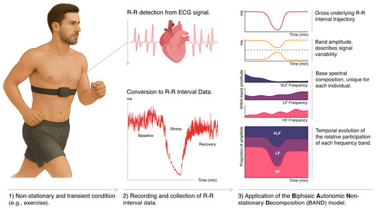
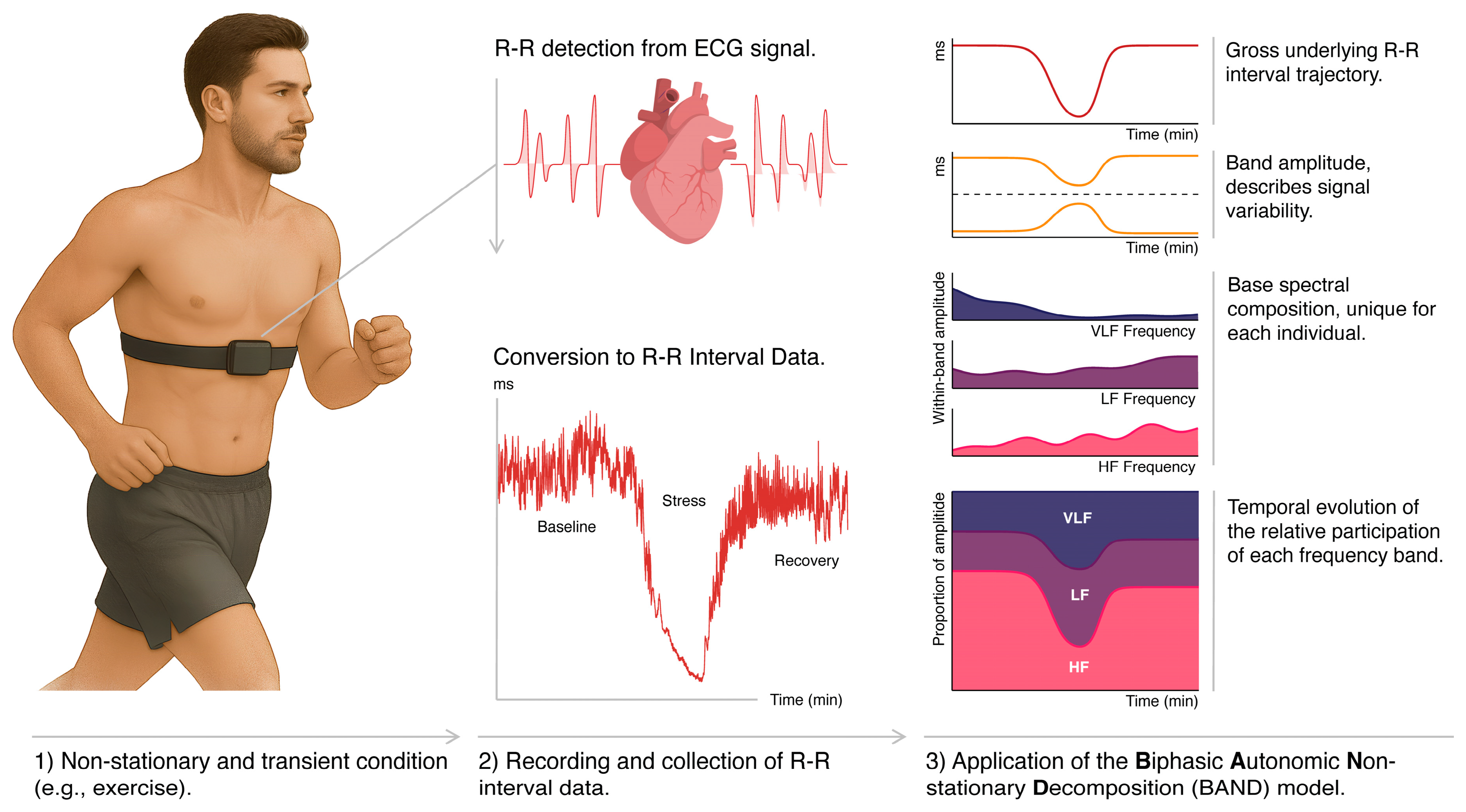
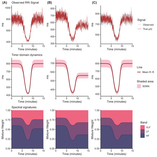
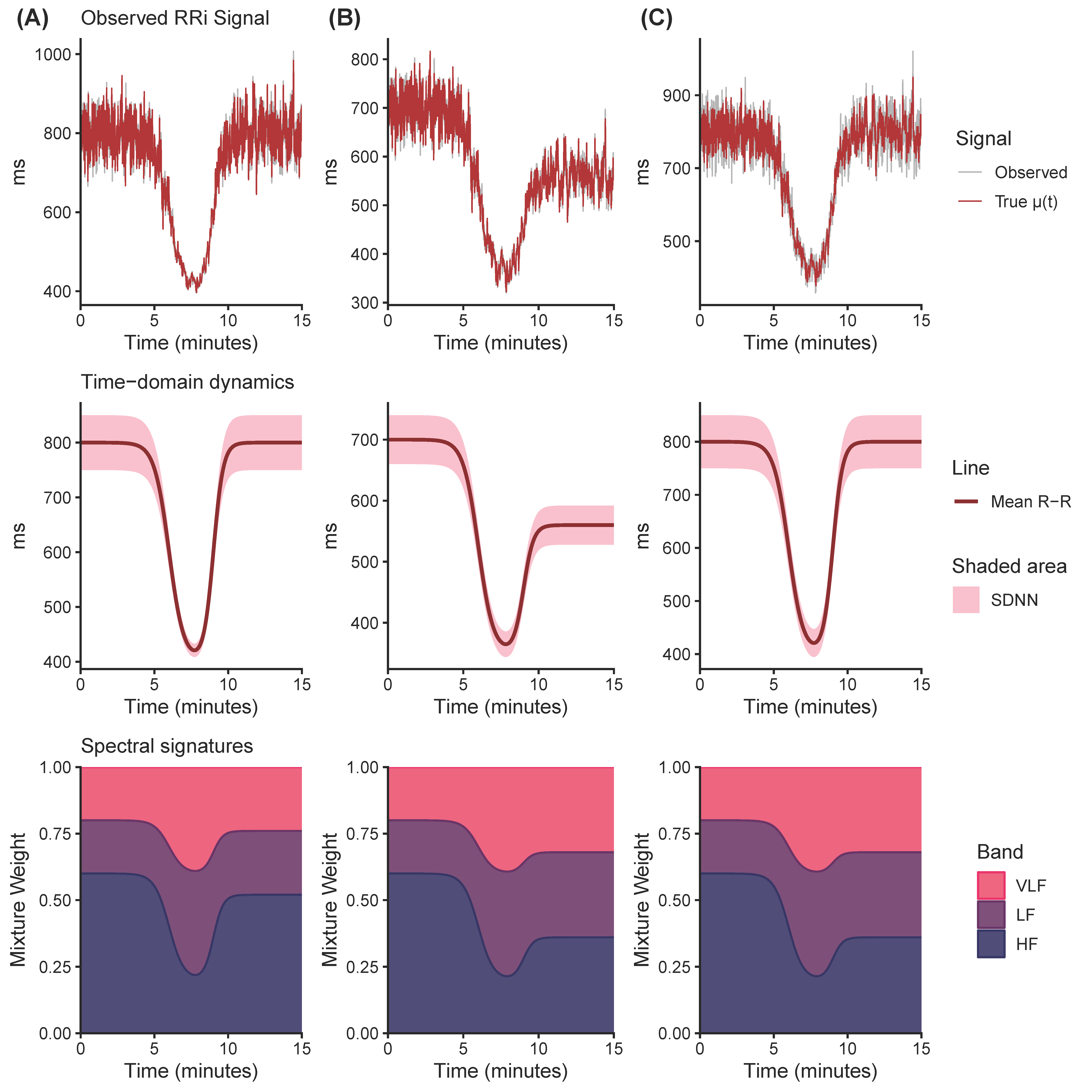
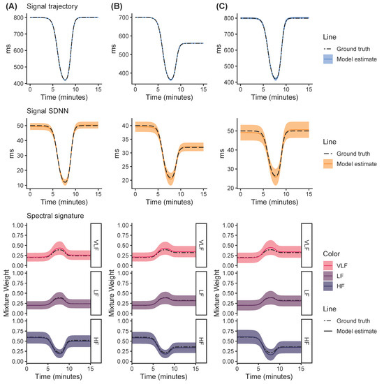
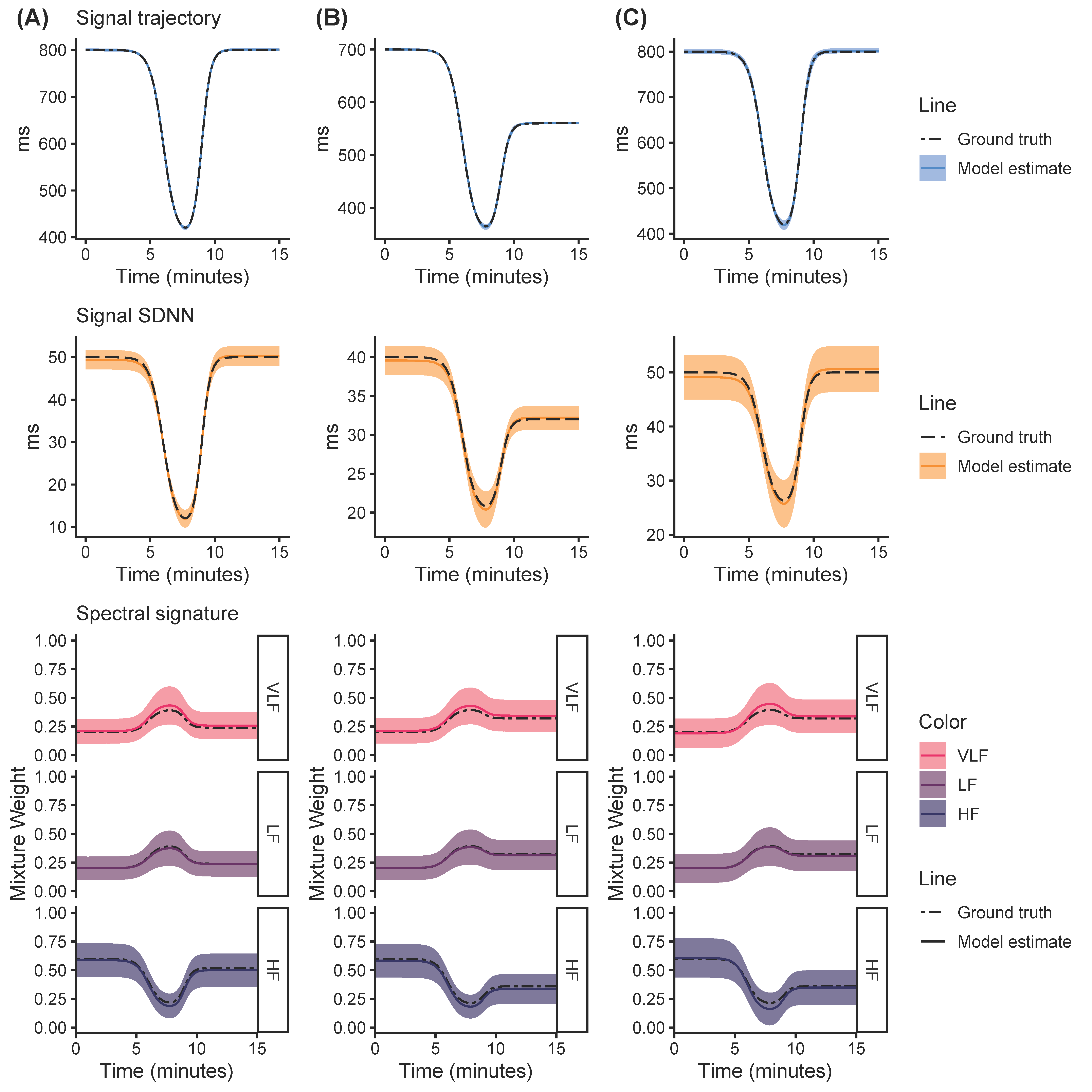
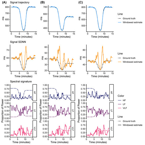
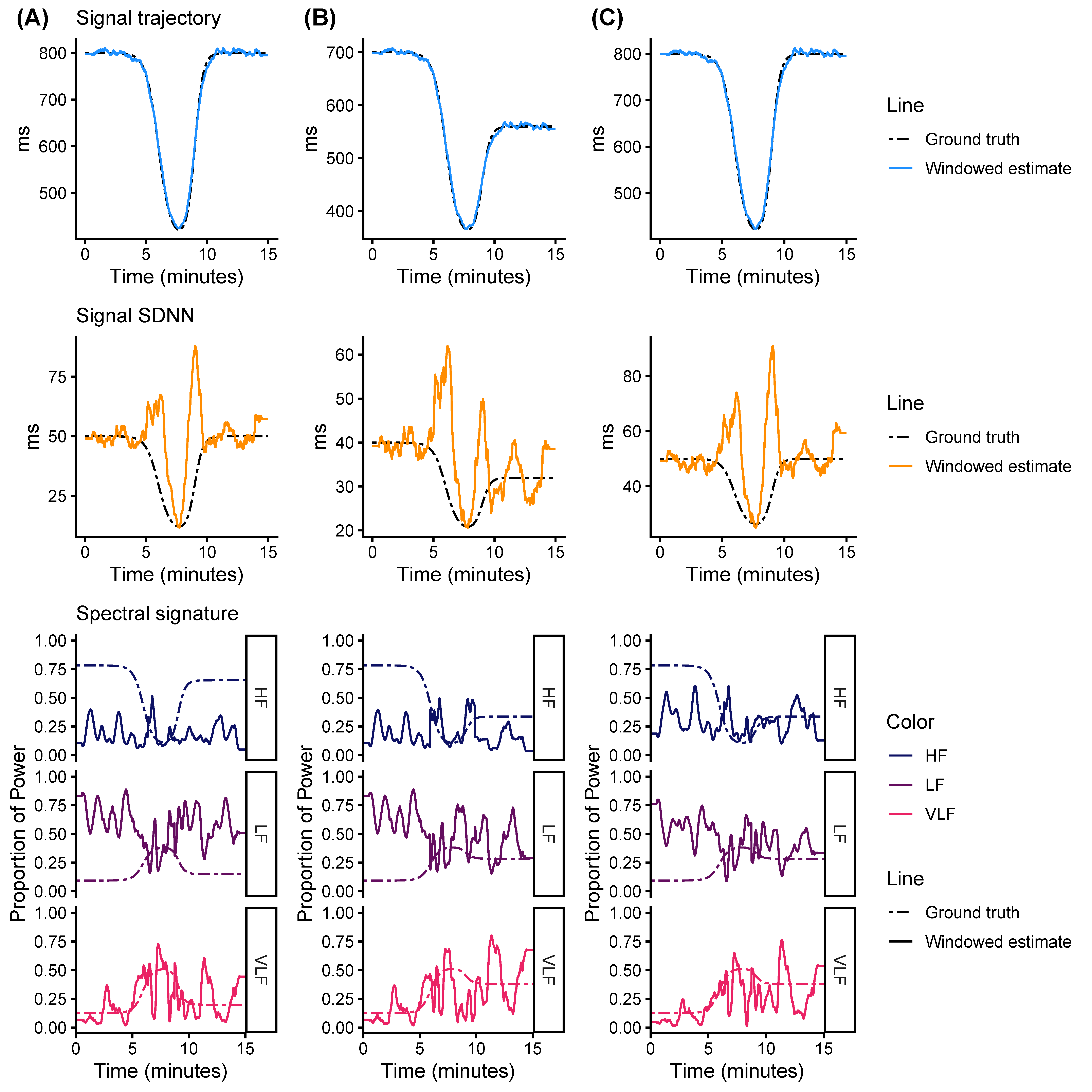
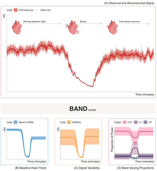
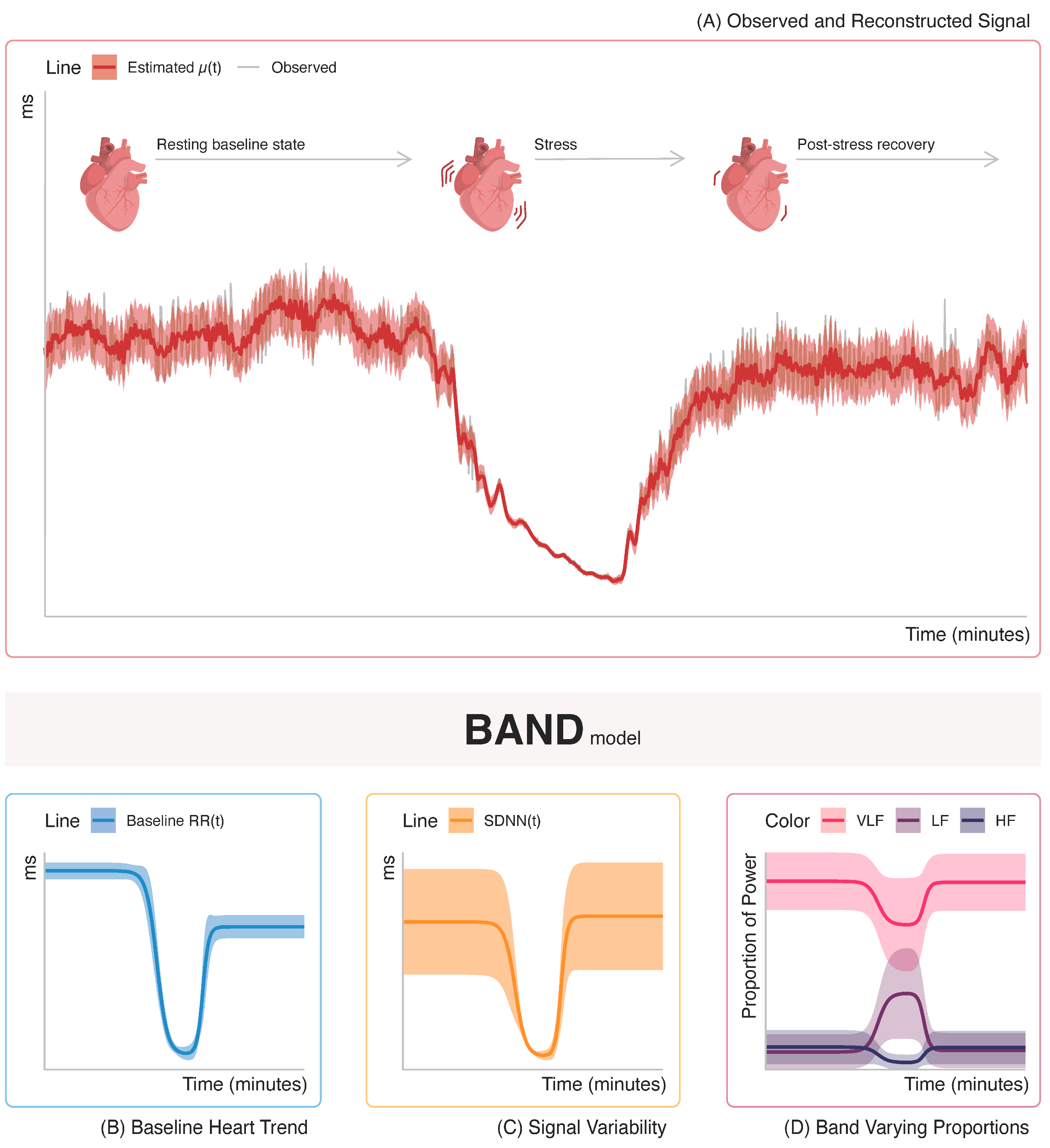
Disclaimer/Publisher’s Note: The statements, opinions and data contained in all publications are solely those of the individual author(s) and contributor(s) and not of MDPI and/or the editor(s). MDPI and/or the editor(s) disclaim responsibility for any injury to people or property resulting from any ideas, methods, instructions or products referred to in the content. |
© 2026 by the authors. Licensee MDPI, Basel, Switzerland. This article is an open access article distributed under the terms and conditions of the Creative Commons Attribution (CC BY) license.