Prediction of Waterjet Cutting Depth Under Multi-Field Coupling Based on Zero-Shot Learning

Abstract

Sudden collapse accidents in mine roadways occur frequently, and post-disaster emergency rescue faces major challenges in terms of safety and efficiency. Therefore, efficient demolition equipment and intelligent prediction methods are urgently needed. Abrasive waterjet technology has considerable potential for complex disaster environments owing to its high efficiency, environmental friendliness, and cold-cutting characteristics. However, its cutting performance is affected by multiple coupled factors, including jet parameters, material properties, and environmental conditions. This makes accurate prediction difficult, especially under extreme or unseen operating conditions where available samples are limited. To address this problem, this study proposes a zero-shot learning-based multi-physics coupling prediction framework for the “jet–material–environment–effect” relationship. The framework is designed to predict abrasive waterjet cutting performance under unseen working conditions. First, a multi-factor cutting-performance dataset is constructed through a hierarchical experimental design. A generative adversarial network (GAN) is then introduced to expand the sample space and compensate for the discrete nature and limited distributional coverage of the experimental data. Second, a lightweight self-attention mechanism is employed to model high-dimensional input features globally, thereby improving the model’s ability to capture complex feature interactions. Finally, a joint loss function is designed to collaboratively optimize the generation and prediction processes. The experimental results show that the proposed model achieves a prediction accuracy of 98.3% on the test set, with a coefficient of determination R² of 0.967, outperforming WOA-SVM, BP neural network, EML, and Transformer models. The inference response time is approximately 3.2 s, indicating good engineering applicability. The results demonstrate that GAN effectively expands the sample space and improves model generalization, while the LightTransformer structure provides advantages in modeling high-dimensional coupled inputs. The proposed method can provide theoretical support and technical reference for intelligent demolition rescue and cutting-depth prediction under mine disaster conditions.

1. Introduction

As the world’s largest producer and consumer of coal, China produced 4.71 billion tons of coal in 2023, accounting for 51.8% of global output. Coal occupies a dominant position in China’s energy structure and supports national economic development, energy security, and the optimization of the industrial structure [1,2,3,4]. With the increase in coal-mining depth, underground geological conditions have become increasingly complex, and accidents such as roof collapses occur frequently, posing serious threats to life safety [5,6]. The country attaches great importance to the development of mine disaster emergency rescue technologies and promotes the research and development of efficient drilling rescue technologies and equipment [7,8]. Abrasive waterjet cutting technology shows application potential in mine emergency rescue owing to its high efficiency, environmental friendliness, and cold-cutting advantages [9]. However, cutting performance is affected by many parameters. The dynamic instability of high-pressure waterjets, nonlinear control difficulties, and the lag of real-time feedback and sensing mechanisms make it extremely difficult to accurately control the cutting path and depth of waterjets at complex rescue sites. This may cause accidental damage to surrounding structures and lead to secondary collapse, thereby limiting its practical application in rescue operations. To improve the application effectiveness of abrasive waterjet cutting technology in mine emergency rescue, it is urgent to establish a cutting-performance prediction model to achieve accurate prediction and control of the cutting depth.

In recent years, abrasive waterjet technology has attracted extensive attention in the fields of complex material cutting and emergency rescue. Existing studies have mainly focused on the cutting mechanism of waterjets, process-parameter optimization, and the construction of intelligent prediction models. Zhang Wenfeng et al. [10] modeled and analyzed abrasive velocity in the external flow field of abrasive waterjet nozzles based on solid–liquid two-phase flow theory and proposed an abrasive velocity solution method combining the displacement segmentation method and an iterative algorithm. Wang Fengchao et al. [11] concluded from experimental results that traverse speed is the most important factor affecting abrasive jet cutting depth. Zhang Yongjiang et al. [12] carried out theoretical modeling of annular slotting depths by high-pressure waterjet, proposed a slotting-depth calculation method integrating the velocity attenuation law with the maximum elongation linear strain criterion, and constructed a theoretical model for annular slotting depth that comprehensively considers jet pressure, nozzle diameter, and coal mechanical parameters. Qiang Zhengrong et al. [13] used the Eulerian method and a discrete particle model, and applied CFD simulation to explore the three-phase flow inside an abrasive waterjet nozzle, establishing a physical model of the nozzle and revealing the influence mechanisms of abrasive shape and outlet velocity on cutting performance. Guo Jiahe et al. [14] systematically investigated the effects of stand-off distance, jet pressure level, and traverse rate on waterjet cutting efficiency through single-factor and orthogonal experiments, and developed an engineering-applicable prediction equation for jet cutting depth using multiple linear regression. Liu Xin et al. [15] derived a model relating the volume removal of rock by abrasive particles to abrasive velocity, constructed a model for the volume removed by abrasive jet cutting of rock by combining mathematical modeling and theoretical derivation, and proposed an annular abrasive jet-cutting-depth calculation model based on the abrasive-jet kerf shape. Although these methods can simulate the motion state of waterjets under complex operating conditions with relatively high accuracy, they entail high computational costs for complex working conditions involving multiple influencing factors and lack real-time capability, making them unsuitable for emergency rescue sites.

To achieve accurate prediction of cutting performance and low-cost processing, researchers have introduced machine learning methods. Deng et al. [16] addressed the shortcomings of BP neural networks, including slow convergence to local optima and susceptibility to stagnation, by using a genetic algorithm to optimize the initial weights and thresholds of the network, thereby realizing cutting-depth prediction and process-parameter optimization for abrasive waterjet cutting of aluminum alloys. Li et al. [17] combined the whale optimization algorithm with support vector machines to achieve an efficient prediction of rock cutting depth, with R² reaching 0.972. Popan et al. [18] introduced an artificial neural network (ANN) model to effectively predict and optimize the best process parameters for abrasive waterjet cutting of carbon-fiber-reinforced polymer (CFRP) materials, thereby improving cutting efficiency. Mogul et al. [19] developed a back-propagation neural network model for adaptive prediction of cutting depth during abrasive waterjet machining of Ti-6Al-4V alloy. Periyappillai et al. [20] proposed a data-driven ensemble machine learning (EML) model that combines k-nearest neighbors, random forests, long short-term memory (LSTM) networks, artificial neural networks (ANNs), and response surface methodology (RSM) to jointly predict surface roughness and the material cutting rate, significantly improving cutting accuracy and stability in abrasive waterjet cutting of composite materials.

However, existing studies still face three key bottlenecks in predictive modeling for abrasive waterjet cutting. First, most existing machine learning models rely on laboratory steady-state working-condition data and are difficult to generalize to the complex environments of emergency rescue sites. Second, current models generally construct prediction systems for a single homogeneous material, such as pure coal rock or metal plates, and are unable to cope with multiphase composite media at mine rescue sites, such as fractured coal–rock masses containing steel supports or concrete–metal hybrid structures. Third, the response time of existing prediction systems generally cannot meet the real-time control requirements of rescue equipment. These limitations essentially arise from the lack of a multi-source heterogeneous data fusion mechanism and insufficient cross-material coupling modeling capability.

To address these challenges, this study proposes a zero-shot learning framework for modeling the multi-physics “jet–material–environment–effect” relationship. Unlike conventional models developed for a single homogeneous material or a fixed parameter range, the proposed framework combines GAN-based training data augmentation with a lightweight self-attention predictor to generalize across laboratory and field-data domains. In this study, zero-shot learning refers to cutting depth regression for materials and complete operating-condition combinations that are absent from the training set. The main contributions are as follows: (i) hierarchical experiments are conducted to cover homogeneous and composite cutting conditions; (ii) GAN-generated samples are used exclusively to augment the training partition; (iii) LightTransformer captures global interactions among process parameters, material properties and categories, and environmental variables using a simplified encoder structure; and (iv) an entirely real, field-measured test set containing unseen materials and operating-condition combinations is retained for independent evaluation. This design enables cross-condition and cross-material zero-shot regression while maintaining practical relevance to abrasive waterjet cutting under complex field conditions.

2. Jet Cutting Experiments

2.1. Experimental Equipment and Materials

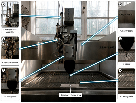
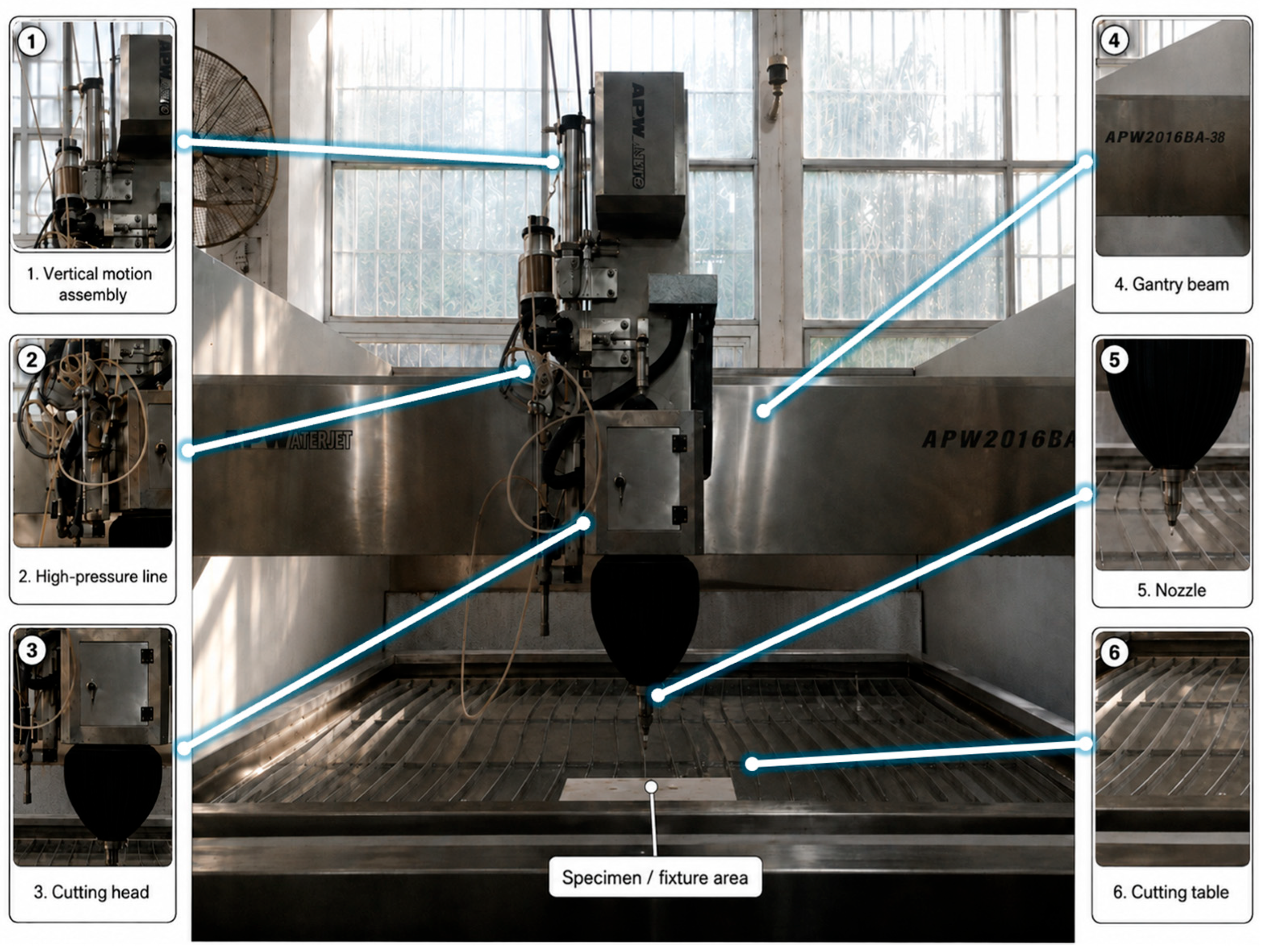
In this study, abrasive waterjet cutting experiments were conducted using an APW2016BA-18 five-axis CNC high-pressure waterjet cutting machine (Shenyang All-Powerful Science & Technology Stock Co., Ltd., Shenyang, China) (Figure 1). The main cutting unit shown in Figure 1 comprises the gantry beam, vertical motion assembly, high-pressure line, cutting head, nozzle, cutting table, and specimen/fixture area. The complete system also includes a high-pressure pump and a CNC control system, which are located outside the field of view of Figure 1. The equipment provides a maximum jet pressure of 420 MPa and is equipped with a 0.33 mm sapphire orifice and a 1.02 mm focusing tube. A post-mixed abrasive waterjet configuration was adopted in the experiments. The principal equipment specifications are summarized in Table 1. The system is capable of conducting controlled cutting tests on different workpiece materials, including metal components and rock specimens.

Figure 1. APW2016BA-18 five-axis abrasive waterjet cutting system.

Table 1. Product specifications of APW2016BA-18 five-axis CNC high-pressure waterjet cutter.

Rated Power (kW)	Maximum Pressure (MPa)	Maximum Flow Rate (L/min)	Pump Frequency (Hz)	Operating Ambient Temperature (°C)
37	420	3.7	50	5–40

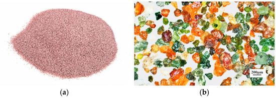
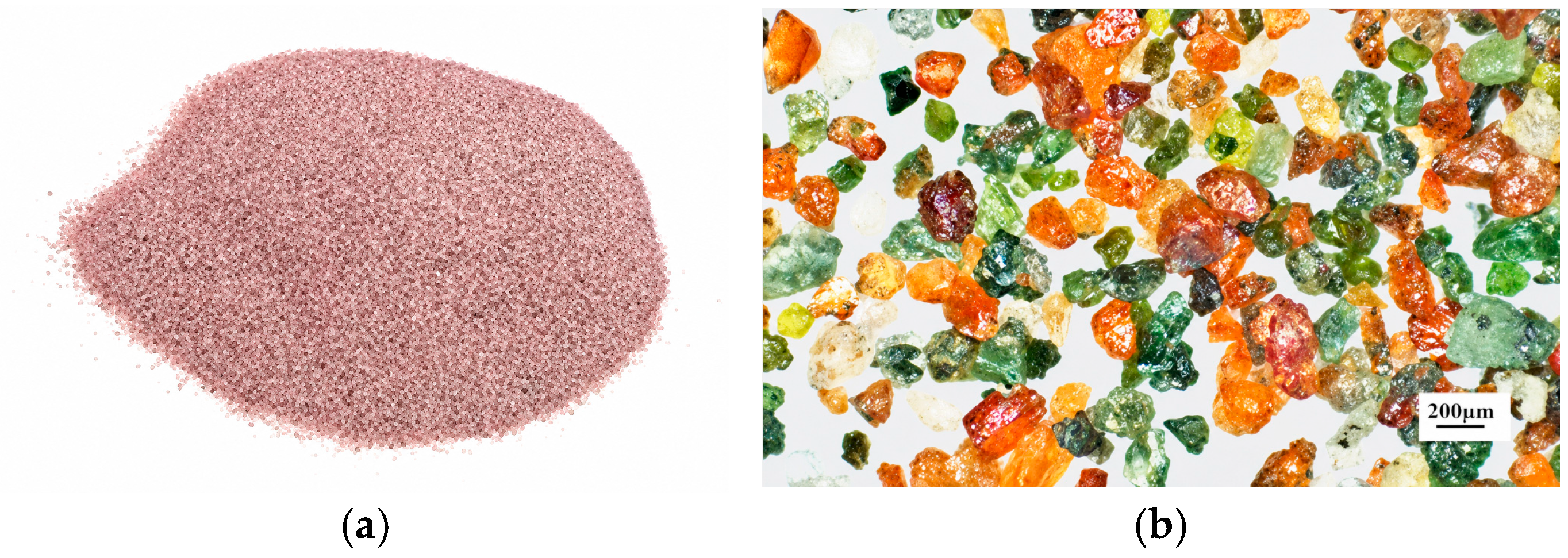
The cutting materials include three types of metal components (I-beam, rock bolt, and anchor cable) and five types of rocks (coal rock, marble, limestone, sandstone, and granite). The abrasive used was 80-mesh garnet particles with an average particle size of approximately 0.18 mm. These particles have sharp edges and irregular morphology (Figure 2), making them suitable for erosion and fragmentation under high-pressure jets.

Figure 2. Schematic diagram of abrasive particle morphology: (a) macroscopic morphology of abrasive particles; (b) microscopic morphology of abrasive particles. Macroscopic appearance and microscopic morphology of the garnet abrasive particles. The reddish-brown, orange, and green colors reflect natural variations in mineral composition and microscopic illumination and do not represent different experimental groups or predefined particle categories.

2.2. Experimental Design

A variety of process parameters are involved in abrasive waterjet cutting. Based on existing studies [21,22,23,24], this study focuses on the influence of cutting passes, traverse speed, abrasive flow rate, cutting angle, and cutting pressure on cutting performance. In addition, considering the effects of cutting materials and environmental factors at emergency rescue sites, variables such as cutting material, stand-off distance, and constraint condition were also set.

Table 2 was constructed as a mixed-level Taguchi design. Cutting passes, traverse speed, abrasive flow rate, and pressure were assigned five levels to cover the available operating range with approximately uniform spacing. Cutting angle was restricted to four physically feasible levels (75°, 80°, 85°, and 90°): angles below 75° caused unstable impingement and excessive lateral splash in preliminary trials, whereas angles above 90° are geometrically equivalent after reversing the traverse direction. The 75° level was therefore repeated in the L25 array to maintain 25 runs and balance the remaining five-level factors. This mixed-level arrangement reflects equipment and safety constraints rather than treating cutting angle as a five-level factor.

Table 2. Orthogonal experiment parameter design table.

Serial Number	Cutting Passes	Traverse Speed (mm/s)	Abrasive Flow Rate (g/min)	Cutting Angle (°)	Cutting Pressure (MPa)
1	1	1	430	75	60
2	1	2	480	80	70
3	1	3	530	85	80
4	1	4	580	90	90
5	1	5	630	75	100
6	2	1	480	85	90
7	2	2	530	90	100
8	2	3	580	75	60
9	2	4	630	80	70
10	2	5	430	85	80
11	3	1	530	80	100
12	3	2	580	85	60
13	3	3	630	90	70
14	3	4	430	75	80
15	3	5	480	80	90
16	4	1	580	90	80
17	4	2	630	75	90
18	4	3	430	80	100
19	4	4	480	85	60
20	4	5	530	90	70
21	5	1	630	85	70
22	5	2	430	90	80
23	5	3	480	75	90
24	5	4	530	80	100
25	5	5	580	85	60

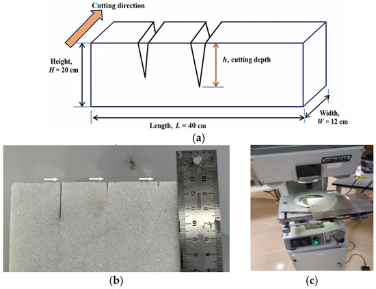
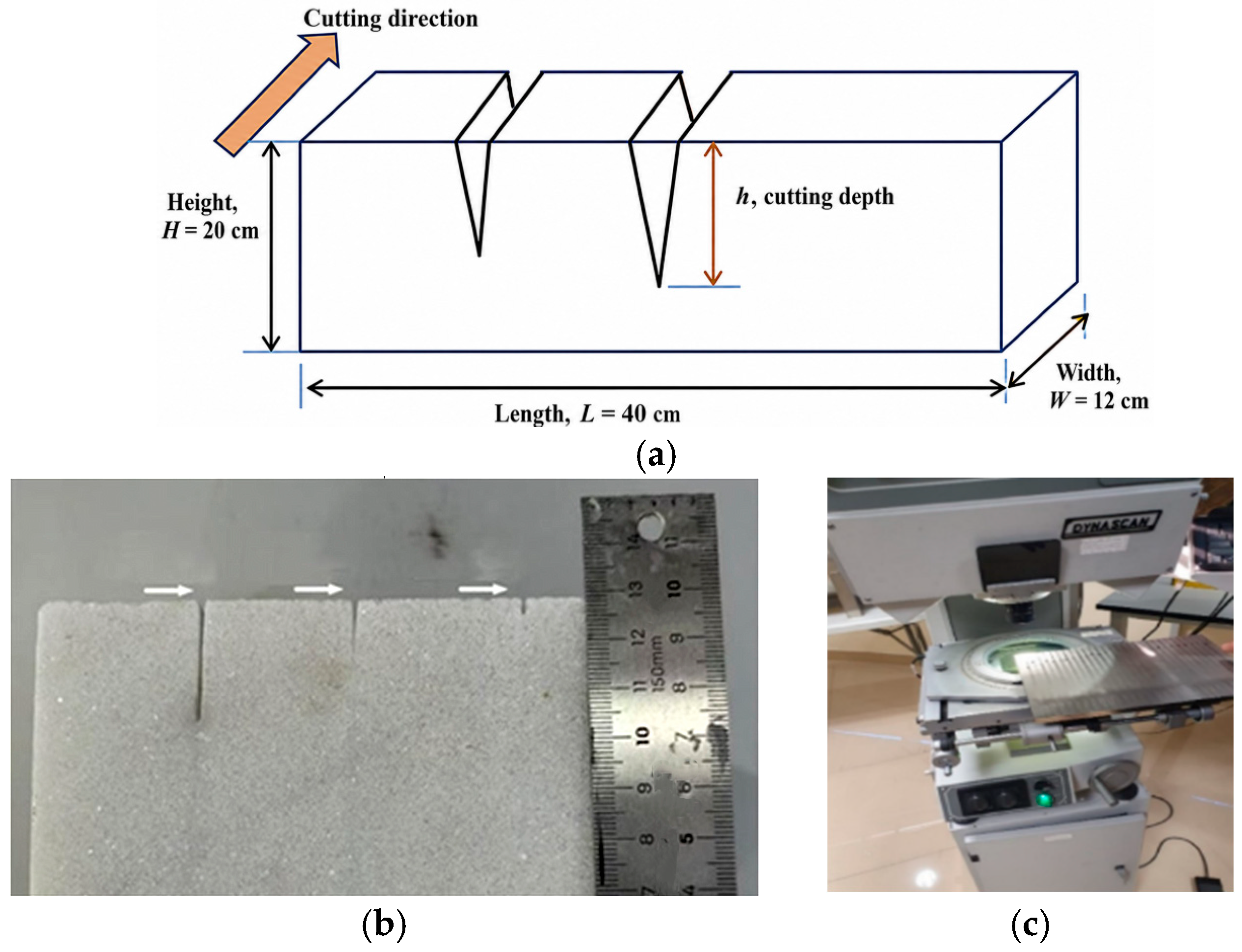
The cutting experiments were conducted using linear slotting. Linear cutting is the most stable cutting mode and helps eliminate interference caused by trajectory complexity under identical working conditions, thereby better revealing the intrinsic influence of key process parameters such as jet pressure, traverse speed, stand-off distance, and cutting angle on cutting depth. All specimens were mounted on the platform using fixing fixtures, and the nozzle impacted the specimen surface vertically or obliquely to achieve stable linear cutting, as shown in Figure 3a. The specimen surfaces were pretreated to remove impurities, and the cutting process was controlled by the CNC system in terms of traverse trajectory and feed speed to ensure experimental repeatability. Three repeated cuts were performed for each parameter configuration, and the cutting depth and profile morphology were recorded and measured. Vernier calipers and a profile projector were used as measurement tools to ensure the accuracy and consistency of the measurement data.

Figure 3. Waterjet cutting experiment: (a) measurement of cutting depth, with the arrows indicating the measurement positions; (b) measurement of cutting depth using vernier calipers; (c) measurement using a profile projector.

Before each run, the pressure was increased from the pump’s unloaded state to the target value and held until the gauge reading stabilized; the traverse speed, abrasive feed, stand-off distance, angle, and number of passes were then entered in the CNC controller according to Table 2 and Table 3. The nozzle origin was calibrated against the specimen surface, the abrasive delivery line was purged, and the fixture was checked for visible displacement. The values in Table 2 were used for the homogeneous material stage, whereas the fixed baseline of 80 MPa, 1 mm/s, 530 g/min, 90°, and one pass in Table 3 was selected as a moderate, repeatable condition for isolating material, distance, and constraint effects.

Table 3. Working condition simulation experiment parameter design.

Condition No.	Material	Environment		Process Parameters
		Stand-Off Distance (mm)	Constraint Condition
1	I-beam + coal rock	5	strong constraint	Cutting passes: 1 Traverse speed: 1 mm/s Abrasive flow rate: 530 g/min Cutting angle: 90° Cutting pressure: 80 MPa Stand-off distance: 5 mm
2	I-beam + marble	5	weak constraint
3	I-beam + limestone	10	strong constraint
4	I-beam + sandstone	10	weak constraint
5	I-beam + granite	15	strong constraint
6	rock bolt + coal rock	15	weak constraint
7	rock bolt + marble	20	strong constraint
8	rock bolt + limestone	20	weak constraint
9	rock bolt + sandstone	25	strong constraint
10	rock bolt + granite	25	weak constraint
11	anchor cable + coal rock	5	strong constraint
12	anchor cable + marble	5	weak constraint
13	anchor cable + limestone	10	strong constraint
14	anchor cable + sandstone	10	weak constraint
15	anchor cable + granite	15	strong constraint
16	I-beam + coal rock	15	weak constraint
17	I-beam + marble	20	strong constraint
18	I-beam + limestone	20	weak constraint
19	I-beam + sandstone	25	strong constraint
20	I-beam + granite	25	weak constraint
21	rock bolt + coal rock	5	strong constraint
22	rock bolt + marble	5	weak constraint
23	rock bolt + limestone	10	strong constraint
24	rock bolt + sandstone	10	weak constraint
25	rock bolt + granite	15	strong constraint
26	anchor cable + coal rock	15	weak constraint
27	anchor cable + marble	20	strong constraint
28	anchor cable + limestone	20	weak constraint
29	anchor cable + sandstone	25	strong constraint
30	anchor cable + granite	25	weak constraint

To ensure that the deep learning model fully learns the complex coupling relationships among the influencing factors from the experimental data and effectively improves prediction accuracy and generalization capability, this study adopts a hierarchical experimental design strategy. The overall experimental process is divided into two stages, namely modeling the parameter influence laws under standard working conditions and training model adaptability under complex working conditions.

The first-stage experiment focuses on the cutting performance of abrasive waterjets on single homogeneous materials, aiming to clarify the influence laws of major process parameters, such as jet pressure, traverse speed, cutting angle, abrasive flow rate, stand-off distance, and cutting passes, on cutting performance. This stage adopts the Taguchi experimental design method [25], a structured experimental design approach that can systematically evaluate the influence of multi-factor and multi-level variables on the output with fewer experimental runs. An L25 orthogonal table was generated using Minitab 19 statistical analysis software, and a test scheme containing 25 experimental combinations was constructed, as shown in Table 2. Each parameter combination was used to perform cutting experiments on eight typical materials, including metal components (I-beam, rock bolt, and anchor cable) and rock materials (coal rock, marble, limestone, sandstone, and granite), thereby obtaining cutting data under different material responses and providing the model with abundant low-noise and high-coverage training samples.

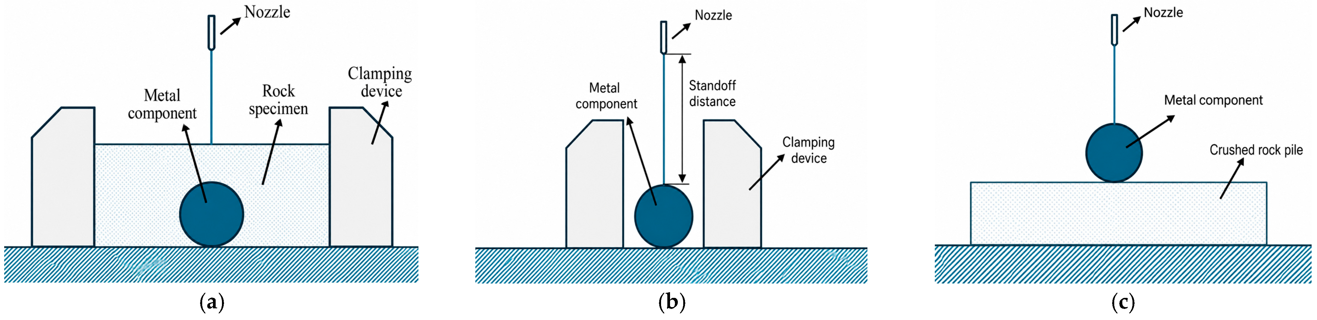
The second-stage experiment targets mine emergency rescue scenarios and simulates cutting tasks under complex environments, thereby further improving the model’s adaptability and prediction stability under real working conditions. Based on the first-stage experiments, this stage introduces material heterogeneity, changes in stand-off distance, and environmental constraint conditions to construct cutting working conditions that are closer to actual rescue needs. The specific experimental combinations for the second stage are shown in Table 3. The design includes three typical scenarios:

(1)

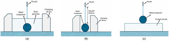
Cross-material cutting: the jet needs to penetrate different types of materials continuously, simulating the situation in which post-disaster support components are mixed and embedded in the collapse body, as shown in Figure 4a;

Figure 4. Schematic diagram of the working condition simulation experiment: (a) cross-material cutting condition; (b) long-distance cutting condition; (c) weak-constraint cutting condition. The blue shaded area represents the cutting platform.

(2)

Long-distance cutting: different stand-off distances are set to simulate the influence of long-distance jetting deep inside boreholes on cutting performance, as shown in Figure 4b;

(3)

Weak-constraint cutting: the cutting specimen is placed in loose sand and gravel piles to simulate a weakly constrained environment in which components in the collapsed area have insufficient supporting force, as shown in Figure 4c.

Through the two-stage experimental design, the parameter influence mechanisms are systematically revealed while the model’s adaptability to complex mine scenarios is enhanced. This ultimately provides comprehensive and reliable experimental data support for constructing a high-precision and robust prediction model for waterjet cutting performance.

3. “Jet-Material-Environment-Effect” Multi-Physics Coupling Prediction Model

3.1. Overall Framework

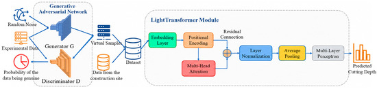
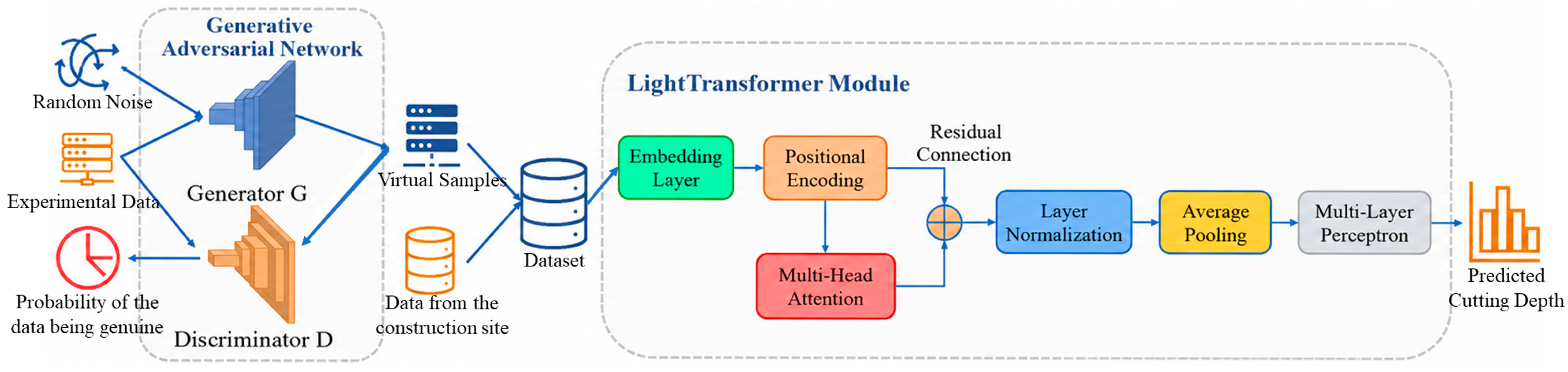
To accurately model and predict the complex nonlinear coupling relationship among “jet-material-environment-effect”, this study constructs a deep learning prediction framework based on a generative adversarial network (GAN) and the LightTransformer model, as shown in Figure 5. The model makes comprehensive use of the rich parameter information and latent distribution features in the experimental data. Through collaborative optimization of generative enhancement and attention mechanism modeling, it improves the prediction accuracy and robustness of cutting performance under different working conditions.

Figure 5. Multi-physics coupling prediction framework of “Jet–Material–Environment–Effect”.

3.2. Generative Adversarial Network (GAN)

Zero-shot learning is a machine learning method that allows a model to make accurate predictions for categories or working conditions that have not appeared during training. Its core idea is to achieve generalization from seen to unseen cases through knowledge transfer and generative modeling, enabling the model to maintain reasonable discriminative ability when facing labels or tasks not covered by the training set, thereby improving adaptability to rare and extreme working conditions.

Due to the limitations of experimental platform conditions and research cost, the sample data obtained from existing simulation experiments are mostly concentrated at discrete parameter-combination points and cannot fully represent the continuously varying process-parameter space in real working conditions. In actual cutting operations, however, key parameters such as jet pressure, traverse speed, and stand-off distance exhibit dynamic and continuous variations, and the corresponding cutting-depth response also has a continuous mapping characteristic. The contradiction between the discrete sampling nature of physical experiments and the continuous prediction demand of practical engineering may lead models trained only on experimental data to exhibit significant prediction deviations in parameter vacancy zones. To break through the limitation of experimental data sparsity, improve the uniformity of sample distribution, and enhance data expression capability, this study innovatively introduces a generative adversarial network (GAN) as a front-end data enhancement module for the prediction model. High-fidelity virtual samples are generated to achieve continuous coverage of the process-parameter space.

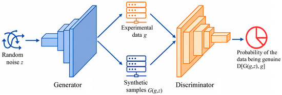
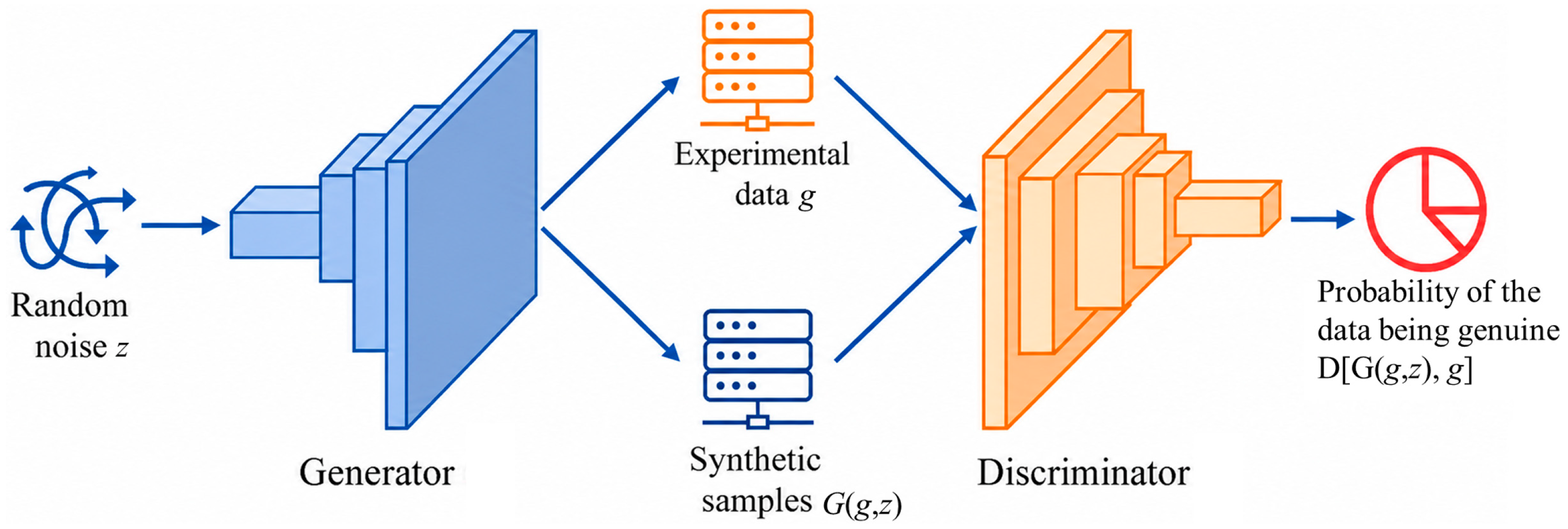
A generative adversarial network consists of a generator and a discriminator and forms an adversarial learning structure, as shown in Figure 6. The generator takes jet parameters, material properties, environmental conditions, corresponding cutting depth, and random noise as inputs, and generates realistic virtual data through a multilayer perceptron neural network. The discriminator receives experimental data and generated virtual data and outputs probability labels indicating whether the data are “real” or “fake”. Through continuous adversarial training, the generator can gradually learn the real distribution characteristics of cutting performance data, thereby generating more representative and diverse samples to expand the model input space and improve overall sample coverage and data diversity. Real laboratory training samples are augmented by the GAN; generated samples remain in the training branch, whereas real-only validation and field-test data are used for model selection and independent evaluation, respectively. The module is designed to address the high-cost and low-throughput sampling limitations in physical experiments while providing broader input combinations for downstream prediction models, which helps the model generalize robustly in complex input spaces. This strategy not only increases the quantity and diversity of training samples, but also theoretically provides data support for cross-condition and cross-material generalization prediction, significantly strengthening the adaptability of the entire prediction framework to complex real-world scenarios.

Figure 6. Schematic diagram of the GAN module structure.

From a physical perspective, the cutting depth depends on both the energy transferred by the abrasive jet and the response of the target material. Increasing jet pressure or abrasive flow generally raises the impact and erosion energy, whereas a higher traverse speed shortens the interaction time between the jet and the target. A longer stand-off distance allows the jet to spread and dissipate energy before reaching the surface, while the cutting angle changes the distribution of normal and tangential impact components. The resulting material removal also varies with thickness, hardness, fracture toughness, and elastic modulus. Harder materials are more resistant to indentation and abrasive erosion, while materials with higher fracture toughness require more energy for crack initiation and propagation. Elastic modulus influences local deformation and load transfer during impact. Under weak constraints, displacement or deformation of the specimen may further reduce the energy effectively used for cutting. These interactions are captured by the attention mechanism from the process parameters, material-property descriptors, stand-off distance, and constraint condition. Here, “multi-physics coupling” refers to a data-driven representation of their combined effects rather than the direct solution of governing physical equations. The physical parameters involved in the paper are shown in Table 4.

Table 4. Physical property descriptors of metal components and rock specimens used in the dataset.

Material	Thickness (cm)	Hardness (HV/Mohs)	KIC (MPa·m1/2)	Elastic Modulus (GPa)
I-beam	10.0	150 HV	75.00	206.0
Rock bolt	22.0	220 HV	55.00	205.0
Anchor cable	17.8	500 HV	40.00	195.0
Coal rock	20.0	2.0 Mohs	0.22	2.5
Marble	20.0	3.0 Mohs	1.20	50.0
Limestone	20.0	3.0 Mohs	0.90	35.0
Sandstone	20.0	6.0 Mohs	0.70	20.0
Granite	20.0	6.5 Mohs	2.20	55.0

3.3. LightTransformer Module

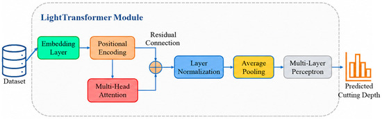
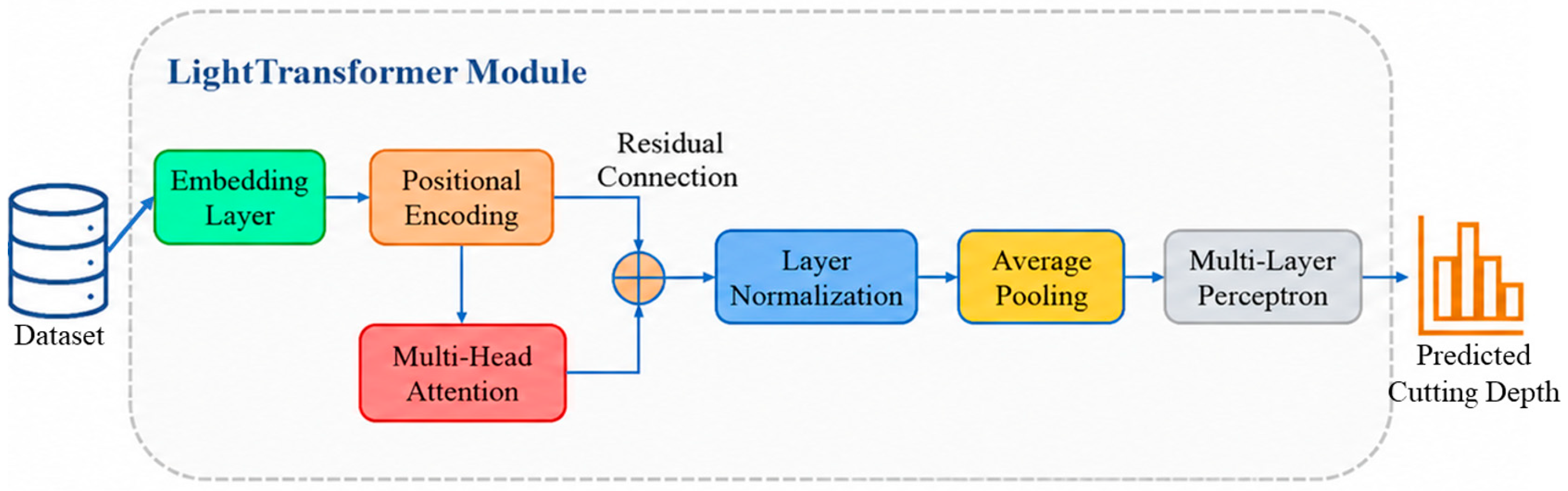
To efficiently model the complex coupling relationships among multi-source inputs such as jet parameters, material properties, and environmental features, this study proposes a LightTransformer module based on a lightweight self-attention mechanism, using the enhanced samples output by the generative adversarial network as input. This module serves as the core prediction network. The LightTransformer module includes an embedding layer, a positional encoding layer, a multi-head attention layer, residual connections, layer normalization, a mean pooling layer, and an output layer. Its network structure is shown in Figure 7.

Figure 7. Schematic diagram of the lightweight self-attention module structure.

The model input is defined as:

$$X=[P,v,q_a,\theta ,s,N_p,c,m_m,t_m,H_m,K_{IC,m},E_m,m_r,t_r,H_r,K_{IC,r},E_r]$$

where $P$, $v$, $q_a$, $\theta$, $s$, and $N_p$ denote cutting pressure, traverse speed, abrasive mass-flow rate, cutting angle, stand-off distance, and number of cutting passes, respectively. $c$ represents the constraint condition. The metal component is described by its encoded type $m_m$, thickness $t_m$, hardness $H_m$, fracture toughness $K_{IC,m}$, and elastic modulus $E_m$. The corresponding rock descriptors are $m_r,$ $t_r,$ $H_r,$ $K_{IC,r},$ and $E_r$.

Retaining the metal and rock properties as separate inputs is particularly important for composite cutting conditions because their distinct mechanical responses cannot be adequately represented by a single material-category code or an averaged equivalent property. The resulting input contains 17 variables, each mapped to a 64-dimensional feature representation. Multi-head attention is implemented using four heads with 16 dimensions per head, allowing the model to capture interactions among the operating parameters, material properties, and constraint conditions. The features of the 17 input tokens are subsequently aggregated by mean pooling and passed to the final linear regression layer. This compact structure avoids the stacked encoder blocks and position-wise feed-forward networks used in a conventional Transformer.

$$\begin{array}{c}{x}^{\prime }=x+PE\end{array}$$

(1)

$$\begin{array}{c}\mathrm{Attention}\left(Q,K,V\right)=\mathrm{softmax}\left({\displaystyle \frac{Q{K}^{\mathsf{{\rm T}}}}{\sqrt{d_K}}}\right)V\end{array}$$

(2)

$$\begin{array}{c}\mathrm{MultiHead}\left(Q,K,V\right)=\mathrm{Concat}\left({\mathrm{head}}_1,\dots ,{\mathrm{head}}_h\right)W^O\end{array}$$

(3)

$$\begin{array}{c}{x}^{″}=LayerNorm\left(x^{\prime }+\mathrm{MultiHead}\left(x^{\prime }\right)\right)\end{array}$$

(4)

$$\begin{array}{c}\overline{x}={\displaystyle \frac{1}{n}}{\displaystyle {\displaystyle \sum }_{i=1}^n}{x}_i\end{array}$$

(5)

$$\begin{array}{c}\widehat{y}=MLP\left(\overline{x}\right)\end{array}$$

(6)

In the equations, x denotes the model input, n denotes the number of variables, and d denotes the embedding dimension of each variable; PE denotes positional encoding; Q, K, and V denote Query, Key, and Value, respectively; $W^O$ is a learnable linear transformation matrix used to map the multi-head attention output back to the original model dimension; $x^{″}$ denotes the output of layer normalization; $\overline{x}$ denotes the output of the mean pooling layer, which is a global feature vector integrating information from all input variables; and $\widehat{y}$ denotes the predicted cutting depth of the waterjet.

While preserving the strong global modeling capability of Transformer, LightTransformer optimizes and prunes the network structure to improve computational efficiency and reduce parameter redundancy. It is especially suitable for industrial prediction tasks with limited experimental data, clear structure, and known semantic positions. Compared with the conventional Transformer, LightTransformer removes the position-wise feed-forward networks and stacked encoder blocks while retaining multi-head self-attention as the main feature-interaction module. Each input variable is mapped to a fixed 64-dimensional representation, and the attention output is combined with the original representation through a residual connection followed by layer normalization. Mean pooling is then applied across the input tokens before the final regression layer. This compact structure reduces the number of repeated feature transformations and lowers the computational costs of both training and inference. This substantially reduces computational complexity and training costs. Such structural simplification not only reduces redundant feature transformations and accelerates convergence, but also avoids overfitting risks, making it particularly suitable for regression prediction tasks with structured inputs.

In addition, because the original Transformer structure lacks awareness of input order and its attention mechanism is essentially position-independent, positional encoding is still needed in the LightTransformer module to supplement sequence-structure information. In this study, the input parameters have clear physical meanings and a fixed order; for example, the first dimension is jet pressure, the second is traverse speed, and so on. Without positional encoding, the model would be unable to identify the position of each input dimension in the sequence and its corresponding physical attribute, leading to insufficient understanding of structural dependencies among input variables by the attention mechanism. Therefore, this paper adopts learnable positional embeddings, enabling the model to automatically acquire semantic position information of each parameter in the input sequence and thereby improve its ability to model causal relationships among variables. Through the above structural optimization, LightTransformer combines a small parameter scale with strong modeling capability. It is suitable for modeling high-dimensional dense input data, has good generalization ability, and can effectively improve the response performance and stability of the multi-physics prediction framework under complex working conditions.

3.4. Joint Loss Function Design

To achieve efficient collaborative optimization of the generation module and the prediction module within a unified training framework, and to improve the model’s ability to represent and predict cutting performance under complex working conditions, this study designs a joint loss function as the overall optimization objective. The joint loss function consists of two parts: the adversarial generation loss for the GAN, which guides the generator to produce virtual samples that better match the real data distribution; and the regression loss for the LightTransformer module, which measures the numerical deviation between the model output and the real cutting performance. Embedding these two types of loss functions in the same training process enables simultaneous optimization of sample distribution learning and functional-mapping learning.

Specifically, the adversarial generation loss uses cross-entropy loss as the core metric. Its objective is to maximize the discriminator’s accuracy in identifying real samples and minimize the probability that generator outputs are classified as fake samples. The generator aims to produce pseudo cutting samples that are as realistic as possible to deceive the discriminator, while the discriminator attempts to distinguish real samples from generated samples, thereby continuously improving the generator’s ability to learn the data distribution. This process encourages the generator to approximate the latent distribution of the real data, alleviates the insufficiency caused by discreteness in the experimental data parameter space, and further enhances the model’s generalization ability under continuous working conditions. The regression loss adopts mean squared error (MSE) as the core metric. Its objective is to minimize the numerical difference between the predicted value and the real cutting performance under given input parameter conditions, thereby improving prediction accuracy in practical tasks.

To balance the optimization weights of the two objectives, the joint loss function is defined as:

$$\begin{array}{c}{L}_{\mathrm{total}}={\lambda }_1·L_{\mathrm{GAN}}+{\lambda }_2·L_{\mathrm{MSE}}\end{array}$$

(7)

$$L_{\mathrm{GAN}}=-E_{z~p_z(z)}[\log D(G(g,z),g)]$$

(8)

$$L_{\mathrm{MSE}}={\displaystyle \frac{1}{N}}{\displaystyle \sum _{i=1}^N{(y_i-{\widehat{y}}_i)}^2}$$

(9)

where L denotes the joint loss function; LGAN is the adversarial generation loss term; LMSE is the regression loss term; and λ1 and λ2 are adjustable weighting coefficients used to control the relative contributions of generation accuracy and prediction accuracy. During training, the weighting coefficients can be dynamically adjusted according to validation-set performance to achieve optimal coupling between the loss terms. E denotes mathematical expectation; g is the sample input to the generator; z is a random noise vector; pz(z) is the noise distribution; G denotes the sample output by the generator; D denotes the discriminator output; N is the number of samples; y is the true value; and ŷ is the model prediction. This joint loss structure not only ensures the distributional rationality of samples generated by the GAN module, but also strengthens the regression prediction capability of the LightTransformer module. Thus, it constructs a deeply integrated model with both generative representation and function-fitting capability, providing effective support for high-precision prediction under complex multi-physics input conditions.

4. Experimental Validation

4.1. Dataset

The dataset contains 2000 waterjet cutting records. Of these, 230 were obtained from laboratory experiments, and 1170 were generated by the GAN. These 1400 samples were used for model training. The remaining 600 records were collected under field conditions and divided into a validation set of 200 samples and a test set of 400 samples. Synthetic samples were restricted to the training set, whereas model selection and final evaluation were performed using field data only.

Here, zero-shot learning refers to cutting-depth prediction for materials and complete operating conditions not encountered during training. The training set covers three metal components and five rock types: coal rock, marble, limestone, sandstone, and granite. The field dataset additionally includes dolomite, mudstone, shale, slate, and basalt, all of which are absent from both the laboratory and GAN-generated training data. These unseen rock types occur in 229 field records, including 77 validation samples and 152 test samples. In addition, no field record has the same complete combination of cutting passes, traverse speeds, abrasive flow rates, cutting angles, pressure, stand-off distance, and constraint conditions as a training record, and several field parameters extend beyond the ranges covered during training. Predictions for these cases rely on numerical descriptors of material thickness, hardness, fracture toughness, and elastic modulus rather than material labels alone. Accordingly, zero-shot learning in this study refers to regression under training-unseen materials and operating-condition combinations, rather than conventional semantic attribute-based zero-shot classification.

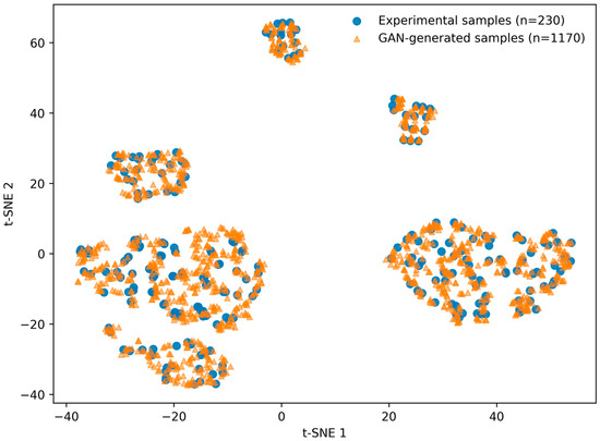
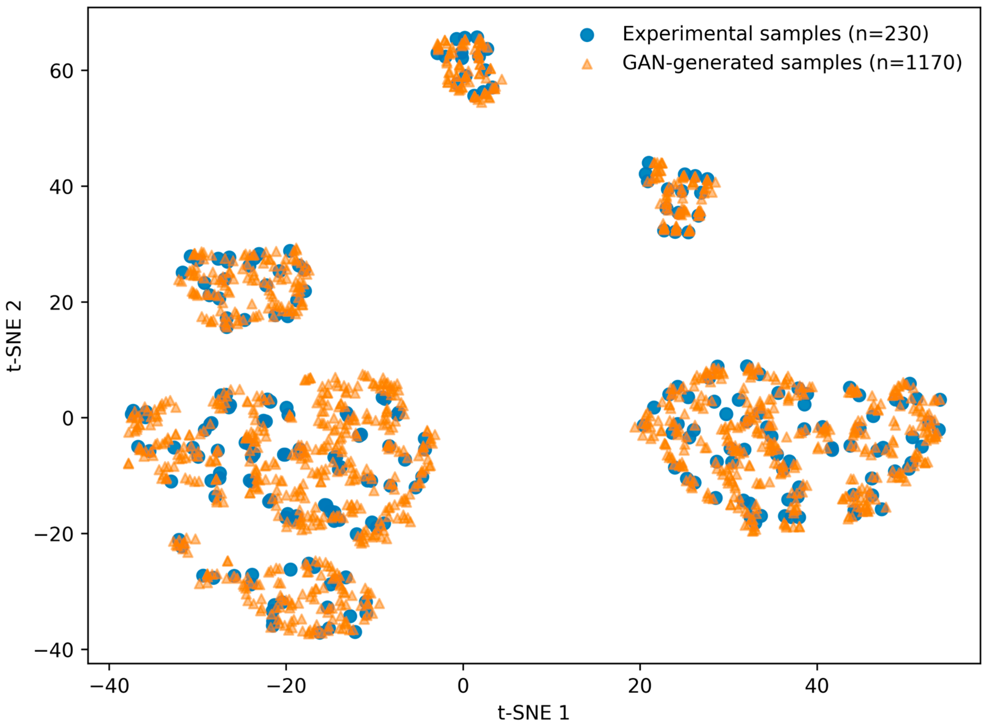
Whether the augmented samples remain close to the experimental data in feature space was examined with t-SNE. The 230 laboratory samples and 1170 GAN-generated samples were standardized and projected into two dimensions using a perplexity of 35, PCA initialization, a fixed random seed of 42, and 1500 iterations. As shown in Figure 8, generated points are interspersed with experimental points across the major local clusters rather than forming a separate synthetic data group. The source-label silhouette coefficient is 0.0039, close to zero, while the trustworthiness score at k = 10 reaches 0.9959. The near-zero source-label silhouette coefficient indicates that the experimental and GAN-generated samples are not clearly separated in the two-dimensional embedding, while the high trustworthiness score suggests that the local neighborhoods of the original feature space are well preserved.

Figure 8. t-SNE visualization of experimental and GAN-generated samples.

4.2. Experimental Settings

The proposed GAN-LightTransformer prediction model was implemented in Python 3.9 based on the PyTorch 1.13.1 framework. The experiments were run on a workstation equipped with an Intel Xeon Gold 6326 processor and two NVIDIA Tesla A100 40 GB GPUs. Model training adopted a staged joint optimization strategy, in which independent hyperparameter settings were configured for the generative adversarial network (GAN) and the LightTransformer prediction module to ensure good convergence and performance for both networks under different learning tasks.

In the first stage, training focuses on the GAN module to learn the latent cutting-performance distribution in the input parameter space. Both the generator and discriminator are trained using the Adam optimizer. The initial learning rate is set to 1 × 10⁻⁴, the β parameters are set to (0.5, 0.999), and the batch size is 64. The discriminator and generator are trained alternately at a 1:1 frequency, and label smoothing and noise perturbation strategies are introduced to improve training stability. This stage ends when the discriminator accuracy for generated samples on the validation set tends to stabilize.

All random seeds and data partitions were fixed before model fitting. GAN training was monitored using the distribution discrepancy between the generated samples and the real validation data. Early stopping was applied when the discrepancy did not improve for a predefined number of consecutive epochs, and the checkpoint with the lowest real-validation distribution discrepancy was retained. The initial weights of the linear layers were initialized using Xavier uniform initialization, while the biases were initialized to zero. Continuous inputs were standardized using the means and standard deviations calculated exclusively from the real training subset, and the same transformation was subsequently applied to the validation and test sets.

In the second stage, training shifts to the LightTransformer module, and the prediction network is jointly trained using real experimental samples and GAN-enhanced samples. This stage also uses the Adam optimizer, with a learning rate of 1 × 10⁻³, weight decay of 1 × 10⁻⁵, batch size of 32, and a total of 300 epochs, as shown in Table 5. An early stopping strategy is enabled to prevent overfitting. Meanwhile, a dropout of 0.2 is introduced in the Transformer encoding module, and learnable positional embeddings are adopted to enhance the model’s structural awareness of the input-parameter order. The prediction output is cutting depth, and the training objective is to minimize the mean squared error (MSE) loss.

Table 5. Training hyperparameter settings of different modules.

Module	Optimizer	Learning Rate	β	Batch Size	Dropout	Epoch
GAN	Adam	1 × 10−4	β = (0.5, 0.999)	64	/	Dyn.
LightTransformer	Adam	1 × 10−3	Decay = 1 × 10−5	32	0.2	300

To comprehensively evaluate the prediction performance of the proposed model, this paper adopts four types of regression metrics as performance evaluation criteria. Mean absolute error (MAE) measures the average deviation between predicted and true values; mean squared error (MSE) reflects the model’s sensitivity to samples with large errors; the coefficient of determination (R²) evaluates the model’s ability to explain data variance; and mean absolute percentage error (MAPE) reflects the overall stability of the model across multi-scale samples. Comparing these metrics among different models on the test set enables a comprehensive verification of the effectiveness and superiority of the proposed method.

4.3. Comparative Experiments

To verify the effectiveness and advantages of the proposed GAN-LightTransformer model in multi-physics cutting-performance prediction, the following five comparison models are selected for evaluation:

WOA support vector machine (WOA-SVM) [18]: a support vector machine combined with the whale optimization algorithm to improve the parameter optimization ability of traditional SVM.

Back-propagation neural network (BPNN) [19]: a classical multilayer perceptron neural network without an attention mechanism, with certain nonlinear fitting capability.

Ensemble learning model (EML) [20]: a model that improves prediction stability and accuracy by integrating multiple base learners.

Transformer [26]: a complete Transformer Encoder structure retaining the encoder and FFN layers, used to evaluate the performance difference between the lightweight model and the original Transformer.

LightTransformer: the prediction model based on the lightweight self-attention mechanism proposed in this study.

All models were developed from the same 230 real laboratory observations and evaluated using the same real-only validation and field-test partitions. To eliminate the influence of unequal training-set sizes, the training set for each model was controlled to contain 1400 samples. For the proposed GAN-LightTransformer, the 230 real laboratory observations were supplemented with 1170 GAN-generated samples. For the other comparison models, the same 230 laboratory observations were expanded to 1400 samples using conventional data augmentation. Conventional augmentation was performed by interpolation between neighboring real samples, followed by small Gaussian perturbations within the experimentally observed parameter ranges. This strategy maintained an equal number of training samples across all models, thereby preventing differences in dataset size from affecting the performance comparison. It also enabled the effectiveness of GAN-based distribution learning to be evaluated against conventional interpolation-and-perturbation augmentation. In particular, the comparison between LightTransformer and GAN-LightTransformer, which share the same prediction-network structure, isolates the contribution of GAN-based augmentation more directly. All generated or conventionally augmented samples were confined to the training set, whereas the validation and test sets consisted entirely of real field data.

All neural network-based predictors, including BPNN, Transformer, LightTransformer, and GAN-LightTransformer, were trained using the Adam optimizer with an initial learning rate of 1 × 10⁻³, a batch size of 32, and a maximum of 300 epochs. Early stopping was applied based on validation MSE, and the checkpoint with the lowest validation MSE was retained for final evaluation on the independent test set. For WOA-SVM and EML, the learning rate, batch size, and epoch settings are not directly applicable; their algorithm-specific hyperparameters were selected using the same validation set and a predefined search procedure. Therefore, comparison fairness was controlled through the same real-data basis, equal training-set size, identical validation and test partitions, consistent preprocessing, and a common model selection protocol.

4.4. Experimental Results and Discussion

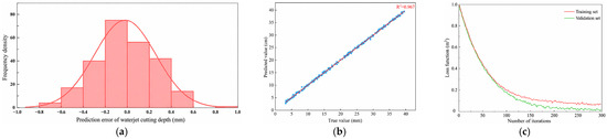
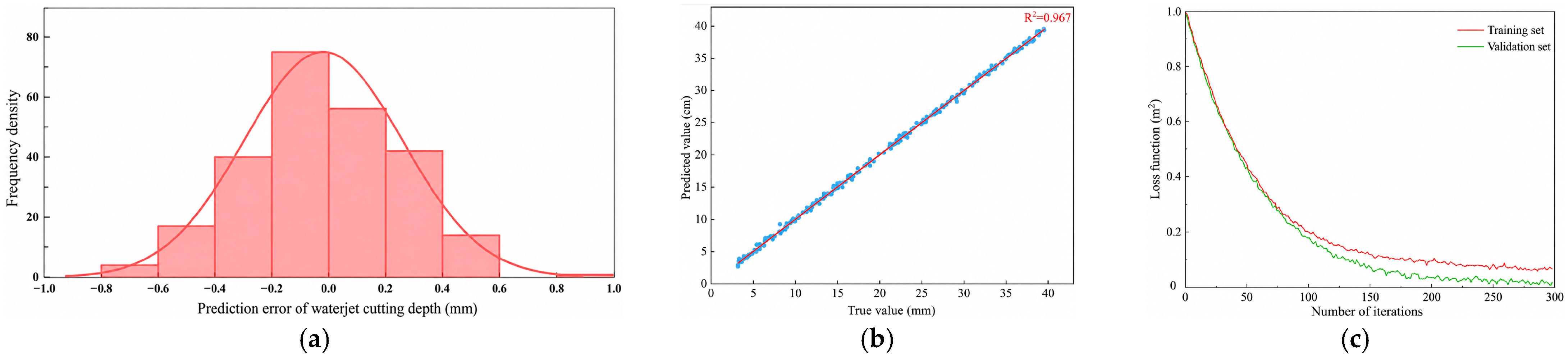
After model training, this paper first systematically evaluated the prediction capability of the proposed GAN-LightTransformer model on the test set to verify its performance in practical applications. Figure 9a shows the error histogram of the model on the test set; the residuals are mainly concentrated within ±1.5 mm, showing good concentration and indicating a stable error distribution. Figure 9b presents the correlation analysis between predicted values and true cutting depths. The coefficient of determination R² of the fitted curve reaches 0.967, demonstrating strong linear consistency. Figure 9c shows the loss convergence curve during training. From the overall trend, the model reaches a stable state within approximately 150 epochs, indicating good training efficiency and convergence of the network structure. In addition, the loss curve of GAN-LightTransformer shows that the trained model’s loss is around 0.08, indicating that both L_GAN and L_MSE remain at relatively low levels. The convergence behavior therefore supports stable joint optimization, while the similarity between generated and experimental sample distributions is assessed independently by the t-SNE analysis in Figure 8.

Figure 9. Prediction performance of GAN-LightTransformer: (a) error histogram, (b) correlation analysis between predicted and true values, and (c) loss function curve.

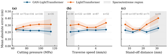
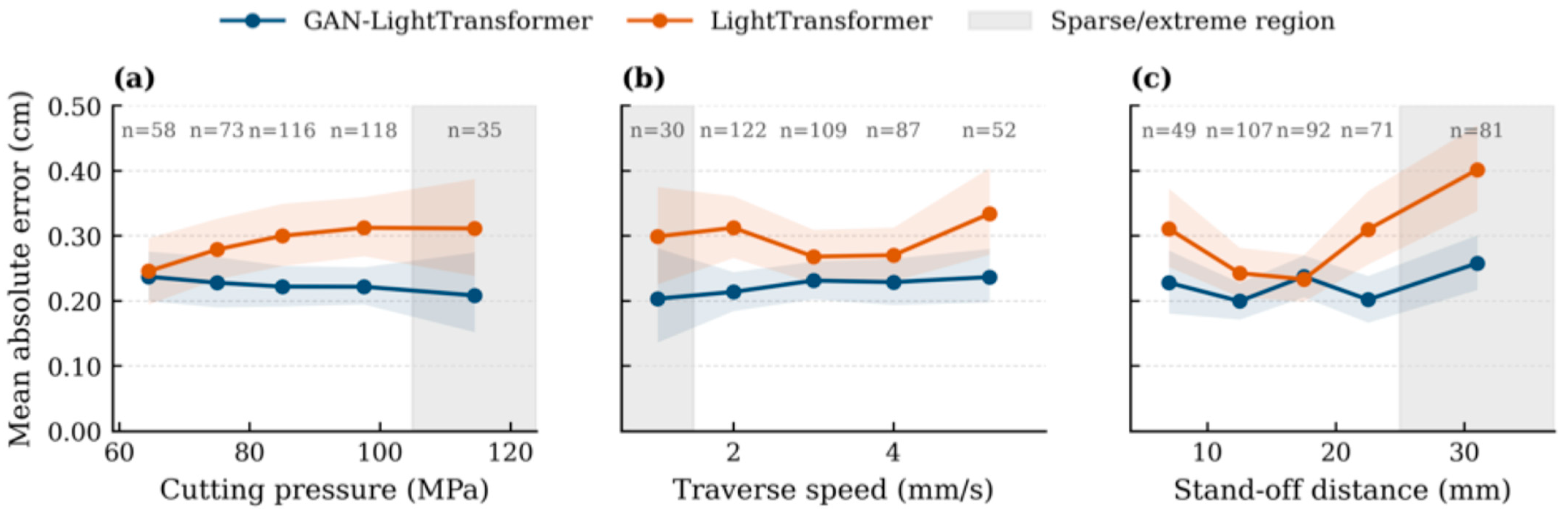
Figure 10 shows how the mean absolute error (MAE) varies with cutting pressure, traverse speed, and stand-off distance. The solid curves represent the mean errors of GAN-LightTransformer and LightTransformer within each parameter interval, while the surrounding shaded bands indicate the corresponding 95% bootstrap confidence intervals. The light gray areas mark relatively sparse or extreme operating regions, including high cutting pressure, low traverse speed, and long stand-off distance. The values of n denote the number of test samples in each interval. GAN-LightTransformer maintains a comparatively stable error level across the three parameters and generally produces a lower MAE than LightTransformer. The difference becomes more apparent in the highlighted regions. Under high-pressure conditions, the error of LightTransformer remains above that of the proposed model, whereas GAN-LightTransformer shows no evident deterioration. A similar pattern appears at low traverse speeds, where the increased cutting intensity and limited sample coverage lead to greater uncertainty for LightTransformer. The influence of stand-off distance is particularly clear: beyond 25 mm, the MAE of LightTransformer rises noticeably, while the increase observed for GAN-LightTransformer is smaller. This behavior suggests that GAN-based augmentation improves the coverage of sparsely sampled operating conditions and reduces the sensitivity of the predictor to shifts in key process parameters. Although some confidence intervals overlap because of the limited number of samples in the tail regions, the overall trends consistently support the improved robustness of GAN-LightTransformer under extreme field conditions.

Figure 10. Relationship between prediction error and key operating parameters in the test set: (a) cutting pressure, (b) traverse speed, and (c) stand-off distance.

In terms of quantitative evaluation, Table 6 compares the performance of the proposed model on the training, validation, and test sets. The model achieved an MSE of 0.052 mm², an MAE of 0.178 mm, a MAPE of 1.21%, and an R² of 0.982 on the training set. On the validation set, the corresponding values were 0.071 mm², 0.213 mm, 1.57%, and 0.971, respectively. When evaluated on the independent test set, the MSE increased slightly to 0.078 mm², while the MAE and MAPE reached 0.224 mm and 1.68%, respectively; the resulting R² remained high at 0.967. Although prediction performance declined gradually from the training set to the validation and test sets, the differences were limited. In particular, the MAE increased by 0.035 mm from the training set to the validation set and by a further 0.011 mm on the test set. The corresponding decrease in R² was 0.011 and 0.004, respectively. This pattern indicates that the model retained most of its predictive capability when transferred from the augmented training distribution to independent field-condition data.

Table 6. Performance of the proposed model on the training, validation, and test sets.

Dataset	MSE (mm2)	MAE (mm)	MAPE (%)	R2
Training set	0.052	0.178	1.21	0.982
Validation set	0.071	0.213	1.57	0.971
Test set	0.078	0.224	1.68	0.967

The observed differences can largely be attributed to the composition and intended use of the three subsets. The training set combined 230 controlled laboratory observations with 1170 GAN-generated samples, providing relatively dense coverage of the parameter combinations used during model fitting. Consequently, these samples were more consistent with the distribution learned by the model and produced the lowest prediction errors. The validation and test sets, in contrast, consisted entirely of real field samples. Variations in material thickness, hardness, fracture toughness, elastic modulus, stand-off distance, and constraint condition introduced a broader and less regular input distribution than that represented by the laboratory data. Field measurements may also contain additional variability arising from specimen heterogeneity, changes in support conditions, and measurement uncertainty. These factors explain the moderate increase in MSE, MAE, and MAPE on the two field-data subsets.

The slightly better performance on the validation set than on the test set is also reasonable because validation data were used to monitor training and select the final model configuration, whereas the test set remained isolated from model development. Moreover, the test set contained 400 samples, twice the size of the validation set, and therefore covered a broader range of field conditions and difficult material combinations. Despite these differences, the test-set R² remained above 0.96 and its MAPE remained below 2%, suggesting that the model did not suffer from a substantial loss of predictive performance when applied to unseen field samples. The relatively small training-to-test performance gap also indicates that restricting GAN-generated samples to the training set did not lead to an unrealistically optimistic evaluation on synthetic data.

Table 7 lists the four major evaluation metrics of this model on the test set, including the mean absolute error (MAE), mean squared error (MSE), mean absolute percentage error (MAPE), and coefficient of determination (R²). The results show that the GAN-LightTransformer model achieves an MAE of 0.224 mm, an MSE of 0.078 mm², a MAPE of 1.68%, and an R² of 0.967, all significantly better than mainstream deep learning and ensemble learning methods. This demonstrates its advantages in modeling the relationship between complex multi-physics input conditions and cutting-performance responses.

Table 7. Evaluation metrics of each model.

Model	MSE (mm2)	MAE (mm)	MAPE (%)	R2
Proposed	0.078	0.224	1.68	0.967
WOA-SVM	0.312	0.425	6.11	0.802
BPNN	0.243	0.388	5.26	0.845
EML	0.184	0.331	4.42	0.891
LightTransformer	0.131	0.293	3.94	0.903
Transformer	0.119	0.256	3.65	0.927

To further compare model performance, this paper selects five representative comparison models: WOA-SVM (whale optimization support vector machine), BP neural network (BPNN), ensemble learning model (EML), Transformer, and LightTransformer. Table 7 lists the four performance metrics of each model on the test set. The results show that the proposed GAN-LightTransformer model performs best in terms of R², MSE, MAE, and MAPE. Specifically, the R² of GAN-LightTransformer is improved by approximately 7.09% compared with LightTransformer, 4.3% compared with Transformer, 8.5% compared with EML, and 20.6% and 14.4% compared with WOA-SVM and BPNN, respectively. In terms of the MSE, it is reduced by 34.5% compared with Transformer and by 75% compared with WOA-SVM, indicating that the model’s error control capability is significantly enhanced. From the perspective of network structure, traditional models such as WOA-SVM and BPNN exhibit obvious underfitting because they lack the ability to model complex nonlinear interactions among high-dimensional input variables. Although EML integrates multiple learners, its sub-models do not form a unified feature-interaction mechanism, and its ability to deeply fuse input information is limited. In contrast, the Transformer model introduces a multi-head self-attention mechanism, substantially improving its ability to capture global dependencies among inputs. GAN-LightTransformer further combines the expansion of the training-sample space by the GAN generation module with the pruning and optimization of structural redundancy by LightTransformer. This not only enhances the diversity of the input distribution but also improves model convergence efficiency and generalization capability. This structural design gives it stronger fitting accuracy and error suppression capability when facing high-dimensional multi-physics inputs.

Table 8 presents the results of the ablation experiment. The complete Transformer achieved the lowest prediction errors, with an MSE of 0.119 mm², an MAE of 0.256 mm, a MAPE of 3.65%, and an R² of 0.927, but required 4.5 s for a single forward prediction. Removing only the FFN reduced the inference time to 3.6 s, a decrease of 20.0%, while the MSE and MAE increased moderately to 0.123 mm² and 0.269 mm, respectively. Its R² remained above 0.91, indicating that multi-head attention and the remaining encoder structure preserved most of the predictive information after the FFN was removed. Further simplifying the network to the LightTransformer reduced the inference time to 2.6 s. Compared with the complete Transformer, this represents a 42.2% reduction in inference time, while the MAPE increased by only 0.29 percentage points and R² decreased by 0.024. The LightTransformer therefore retains useful regression performance despite its substantially shallower structure.

Table 8. Ablation results for the structural simplification of LightTransformer.

Model	MSE (mm2)	MAE (mm)	MAPE (%)	R2	Inference Time (s)
Transformer	0.119	0.256	3.65	0.927	4.5
Transformer without FFN	0.123	0.269	3.77	0.916	3.6
LightTransformer	0.131	0.293	3.94	0.903	2.6

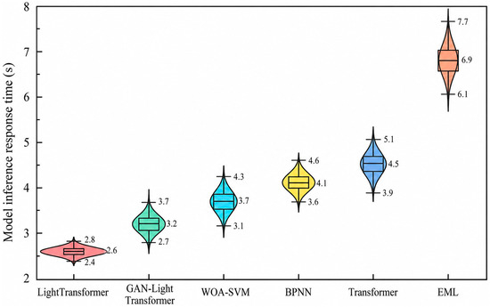
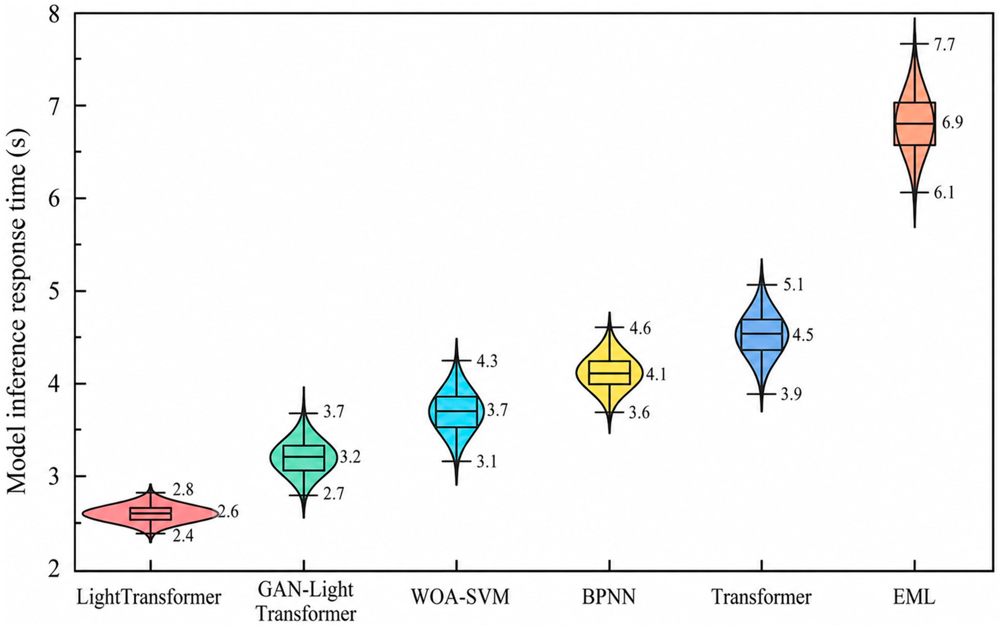
Figure 11 compares the single-sample forward-inference times of the six models using violin plots with embedded summary statistics. The width of each violin reflects the relative density of the measured inference times, with wider regions indicating that more observations are concentrated within that interval. The central horizontal line and its numerical label represent the mean inference time, whereas the lower and upper horizontal markers indicate the 10th and 90th percentiles, respectively. The distance between these two percentile markers therefore provides an intuitive measure of inference time variability. The results show that GAN-LightTransformer has a very fast response speed during inference, with the response time concentrated at 3.2 ± 0.5 s. It is second only to the structurally simple LightTransformer (2.6 ± 0.2 s), slightly faster than WOA-SVM (3.7 ± 0.6 s) and the BP neural network (4.1 ± 0.5 s), and significantly better than the more complex Transformer (4.5 ± 0.6 s) and EML (6.9 ± 0.8 s).

Figure 11. Boxplot of prediction model response time.

The relatively narrow distribution of GAN-LightTransformer shows that its inference time remains stable across repeated predictions. A single prediction takes 3.2 s on average, and 80% of the recorded values lie between 2.7 and 3.7 s. In the intended rescue workflow, the model is used to select cutting parameters before each cutting pass and to revise them when the material combination, stand-off distance, or constraint condition changes. Such adjustments are normally made over periods of seconds or minutes rather than milliseconds. A cutting-depth prediction obtained within approximately 3–4 s should therefore be fast enough to support parameter adjustment without noticeably delaying the cutting operation.

The values in Figure 11 are forward-inference times measured on the computing platform described above; preprocessing, data transmission, and input/output delays were not included. Since the model uses a compact set of numerical process and material descriptors, preprocessing mainly involves data acquisition, encoding, and normalization, without computationally intensive image or signal analysis. The actual end-to-end response time will nevertheless depend on the sensors, communication conditions, and edge-computing hardware available at the rescue site. These factors will be examined in subsequent deployment tests under representative underground conditions. The current results suggest that model inference is unlikely to become the main computational bottleneck and that the predicted cutting depth can be returned within a practical time window for cutting assessment and parameter adjustment.

In summary, GAN-LightTransformer achieves the best prediction accuracy in this task and also has a significant advantage in response speed. Its excellent performance is attributable to two aspects. First, the GAN module enhances the continuity of the data distribution through generated samples and effectively alleviates the discreteness of experimental samples. Second, the LightTransformer structure adopts a lightweight self-attention modeling mechanism, which retains a certain capability for extracting global dependency features while significantly reducing network complexity. This framework shows broad application potential for abrasive waterjet cutting prediction in complex mine environments.

5. Conclusions

Focusing on the problem of cutting-performance prediction in abrasive waterjet demolition operations under mine roadway emergency rescue conditions, this paper proposes a “jet–material–environment–effect” multi-physics coupling prediction framework integrating a generative adversarial network (GAN) and a lightweight self-attention mechanism (LightTransformer). First, cutting-performance data under different materials, parameters, and constraint conditions are obtained through hierarchical experiments, and the GAN module is used for data enhancement to improve input-space coverage. On this basis, a simplified LightTransformer structure is introduced for multi-source feature modeling, and a joint loss function is designed to realize collaborative optimization of generation and regression.

The experimental results show that the proposed GAN-LightTransformer model outperforms the comparison models in both prediction accuracy and inference efficiency. The model achieves a prediction accuracy of 98.3% on the test set and a coefficient of determination R² of 0.967, fully verifying the prediction accuracy and robustness of the proposed method under high-dimensional input parameters. Meanwhile, the average response time of the model during inference is 3.2 ± 0.5 s, showing good lightweight characteristics and engineering deployment potential. Comparative analysis further confirms the important role of GAN-generated samples in alleviating experimental data discreteness and improving model generalization capability. The model’s performance on real tunnel rescue scenario data also demonstrates its strong multi-physics coupling modeling capability and its suitability for predicting complex working conditions in practical engineering.

The principal findings are summarized as follows:

(1)

A hierarchical laboratory-to-field dataset was established to represent interactions among jet parameters, material category, stand-off distance, and constraint states.

(2)

GAN augmentation confined to the training set improved input-space coverage, while real-only validation and field-test partitions preserved independent evaluation.

(3)

The proposed GAN-LightTransformer achieved an MAE of 0.224 mm, MSE of 0.078 mm², MAPE of 1.68%, and R² of 0.967 on the field test set, with an average inference time of approximately 3.2 s on the stated workstation.

(4)

The proposed model can be regarded as a zero-shot learning-based predictor and decision-support tool, as it can estimate cutting depth for materials and operating conditions not represented in the training set. The present results demonstrate its generalization capability under unseen-material scenarios and unseen process-parameter conditions.

The proposed framework provides a basis for modeling the nonlinear relationship among operating conditions, material properties, environmental constraints, and cutting depth in abrasive waterjet rescue operations. Future work will address task-specific scenarios, including steel-support cutting, heterogeneous coal–rock penetration, long stand-off borehole cutting, and weakly constrained collapse debris. Pressure and abrasive-flow signals will be used to monitor jet energy fluctuations, while acoustic, vibration, visual, and depth measurements will support the identification of material transitions, crack development, breakthrough, kerf evolution, and target displacement. These signals can be incorporated at successive cutting stages to update depth predictions and adjust pressure, traverse speed, or cutting passes. Further studies will also examine prediction uncertainty, out-of-distribution inputs, layered metal–rock targets, cross-material generalization, and end-to-end latency on edge devices, supporting the development of an uncertainty-aware decision-support system for mine emergency demolition.

References

- Yuan, L.; Zhang, P. Development Status and Prospects of Geological Guarantee Technology for Precise Coal Mining. J. China Coal Soc. 2019, 44, 2277–2284. [Google Scholar] [CrossRef]
- Xie, H.P.; Ren, S.H.; Xie, Y.C.; Jiao, X.M. Development Opportunities for the Coal Industry under Carbon Neutrality Goals. J. China Coal Soc. 2021, 46, 15. [Google Scholar]
- Wang, S.; Liu, L.; Zhu, M.; Shen, Y.; Shi, Q.; Sun, Q.; Fang, Z.; Ruan, S.; He, W.; Yang, P.; et al. New Ideas for Green and Low-Carbon Development of Coal under the “Dual Carbon” Goals. J. China Coal Soc. 2024, 49, 152–171. [Google Scholar] [CrossRef]
- Cheng, C.; Gao, D.; Zhang, H.; Huang, J.; Xu, Z. Integration Development Scenarios and Key Technologies of Coal and New Energy. Chin. Eng. Sci. 2024, 26, 52–62. [Google Scholar] [CrossRef] [Scilit]
- Sun, T.; Han, J. Coal Mine Dynamic Disaster Accidents and Prevention Measures. Inn. Mong. Coal Econ. 2022, 94–96. [Google Scholar] [CrossRef]
- Li, G.; Cheng, G.; Li, Z.; Zhu, W.; Wu, F. Visualization Analysis of Emergency Rescue Research for Chinese Mines Based on Bibliometrics. Coal Mine Saf. 2023, 54, 253–259. [Google Scholar] [CrossRef]
- Chen, Y.; Yang, W.; Zhang, D. Research Status and Development Trend of Regional Mine Emergency Rescue Systems. China Coal 2020, 46, 57–61. [Google Scholar] [CrossRef]
- Zhou, J. Study on Drilling Technology of Life Guarantee Boreholes for Mine Disaster Emergency Rescue. Drill. Eng. 2022, 49, 128–134. [Google Scholar]
- Zhang, X.; Ma, H.; Chen, G. Research Status and Development Trend of Intelligent Rescue Demolition Technology and Equipment. China Saf. Sci. J. 2025, 21, 211–218. [Google Scholar]
- Zhang, W.; Li, Y.; Tang, J. Abrasive Velocity Model and Analysis of Abrasive Jet Nozzle External Flow Field. J. China Coal Soc. 2017, 42, 576–584. [Google Scholar] [CrossRef]
- Wan, F. Study on Dynamic and Static Stress-Strain Distribution of Abrasive Slurry Jet Impacting Rock. Ph.D. Thesis, China University of Mining and Technology, Xuzhou, China, 2018. [Google Scholar]
- Zhang, Y.; Guo, S. Theoretical Model and Application of Depth for High-Pressure Water Jet Annular Cutting. J. China Coal Soc. 2019, 44, 126–132. [Google Scholar] [CrossRef]
- Qian, Z.; Ma, Y.; Ma, X. Study on Particle Roundness Effect in Abrasive Water Jet Processing Based on CFD. Lubr. Seal. 2020, 45, 62–67. [Google Scholar]
- Guo, J.; Qi, X.; Wang, D.; Zhu, G.; Chen, L. Influencing Factors and Cutting Depth Prediction Model of Abrasive Water Jet Cutting. J. China Saf. Sci. 2020, 30, 101–106. [Google Scholar] [CrossRef]
- Li, X.; Xu, H.; Gao, H. Depth Calculation Model of Abrasive Water Jet Rotational Cutting of Rock. J. Army Eng. Univ. 2022, 1, 77–85. [Google Scholar]
- Deng, S.S.; Guo, L.H.; Guan, J.F.; Guo, G.D.; Yang, X. Research on the prediction model for abrasive water jet cutting based on GA-BP neural network. Chem. Eng. Trans. 2016, 51, 1297–1302. [Google Scholar]
- Li, Z.; Ge, Z.; Deng, Q.; Zhou, Z.; Zhu, C.; Liu, L.; Yao, Z. Predicting the depth of rock cutting by abrasive water jet using support vector machine optimized with whale optimization algorithm. Phys. Fluids 2024, 36, 126633. [Google Scholar] [CrossRef] [Scilit]
- Popan, I.A.; Bocăneț, V.I.; Softic, S.; Popan, A.I.; Panc, N.; Balc, N. Artificial Intelligence Model Used for Optimizing Abrasive Water Jet Machining Parameters to Minimize Delamination in Carbon Fiber-Reinforced Polymer. Appl. Sci. 2024, 14, 8512. [Google Scholar] [CrossRef] [Scilit]
- Mogul, Y.I.; Mogul, I.; Quadros, J.D.; Mohin, M.; Aabid, A.; Baig, M.; Malik, M.A. Prediction of cutting depth in abrasive water jet machining of Ti-6AL-4V alloy using back propagation neural networks. Results Eng. 2025, 25, 104520. [Google Scholar] [CrossRef] [Scilit]
- Periyappillai, G.; Subbarayan, S.; Sengottaiyan, S. Advanced ensemble machine learning prediction to enhance the accuracy of abrasive waterjet machining for biocomposites. Mater. Chem. Phys. 2025, 333, 130175. [Google Scholar] [CrossRef] [Scilit]
- Wei, J.P.; Xiao, P.W.; Zhang, H.D.; Chen, C.J.; Liu, Y. Research on Optimal Parameter Matching Model for Abrasive Water Jet Rotational Cutting of Coal and Rock. Coal Sci. Technol. 2025, 53, 192–202. [Google Scholar]
- Zhu, J.; Tang, K.; Zhang, J.; Li, Y.; Jiang, W. Design Study of an Internal-Curl Cutting Robot for Offshore Rock-Socketed Steel Pipe Piles. Pet. Mach. 2024, 52, 48–59. [Google Scholar] [CrossRef]
- Perec, A. Desirability Function Analysis (DFA) in Multiple Responses Optimization of Abrasive Water Jet Cutting Process. Rep. Mech. Eng. 2022, 3, 11–19. [Google Scholar] [CrossRef] [Scilit]
- Karmiris-Obratański, P.; Karkalos, N.E.; Kudelski, R.; Papazoglou, E.L.; Markopoulos, A.P. On the Effect of Multiple Passes on Kerf Characteristics and Efficiency of Abrasive Waterjet Cutting. Metals 2021, 11, 74. [Google Scholar] [CrossRef] [Scilit]
- Quadros, J.D.; Khan, S.A.; Antony, A. Base Pressure Behaviour in a Suddenly Expanded Duct at Supersonic Mach Number Regimes using Taguchi Design of Experiments. Mech. Mech. Eng. 2018, 22, 1077–1097. [Google Scholar] [CrossRef] [Scilit]
- Vaswani, A.; Shazeer, N.; Parmar, N.; Uszkoreit, J.; Jones, L.; Gomez, A.N.; Kaiser, L.; Polosukhin, I. Attention is All You Need. In Proceedings of the 31st Conference on Neural Information Processing Systems (NIPS 2017), Long Beach, CA, USA, 4–9 December, 2017; Curran Associates Inc.: Red Hook, NY, USA, 2017; Volume 30, pp. 5998–6008. [Google Scholar]
Disclaimer/Publisher’s Note: The statements, opinions and data contained in all publications are solely those of the individual author(s) and contributor(s) and not of MDPI and/or the editor(s). MDPI and/or the editor(s) disclaim responsibility for any injury to people or property resulting from any ideas, methods, instructions or products referred to in the content. |
© 2026 by the authors. Licensee MDPI, Basel, Switzerland. This article is an open access article distributed under the terms and conditions of the Creative Commons Attribution (CC BY) license.