


Abstract
We present ESNformer, a hybrid architecture that couples an Echo State Network (ESN) reservoir with a Transformer encoder for classification of structured, multi-indicator assessment data: a fixed-order vector of complementary indicators per assessment instance rather than a repeated-measures time series. The reservoir acts as a fixed nonlinear feature map over the indicator vector, while self-attention, made position-aware over the fixed column order, learns how each indicator’s evidence contributes to the final decision, so the two components, together, capture local, indicator-level detail and global, cross-indicator interactions within a single, end-to-end trainable model. Interpretability is treated as a first-class design requirement rather than an afterthought: the architecture is paired with an explainability layer combining SHAP feature attribution (reported both globally and per class), the model’s own attention weights, a deletion/insertion faithfulness test that quantitatively verifies which inputs the model actually relies on, and counterfactual maps that translate a prediction into an actionable, inspectable recommendation. We evaluate the architecture on a concrete case study, classifying Braille-literacy instructional recommendations from 15 pedagogical indicators grouped into three categories (Mangold’s, ABKL, and Progresar), using a benchmark of 900 real assessment instances (630 used, together with a class-conditional augmentation procedure, to build a 2100-instance training set) with validation and test partitions (135 instances each) kept exclusively real. On this benchmark, the tuned model reached 85.33% accuracy, 85.90% macro-precision, 85.33% macro-recall, an F1 score of 85.25%, and an AUC of 0.95 on the real test set. SHAP attribution, attention weights, and the faithfulness test converge on the same two dominant indicators (response time and error count): removing them alone collapses accuracy to chance, while retaining only them recovers most of the model’s accuracy. We report this transparently alongside a comparison against ESN-only, Transformer-only, and tabular baselines (logistic regression, decision tree, random forest, XGBoost, and an MLP) on the same data and discuss what the hybrid architecture and its explainability pipeline add beyond what the two dominant indicators already explain and how the approach generalizes to other tabular and mixed-granularity assessment settings that require both predictive accuracy and a verifiable account of what drove each decision.
1. Introduction
Classification of structured, multi-indicator assessment data—a fixed-order vector of complementary measurements per instance, grouped into a small number of outcome categories—is a recurring problem across applied computing, from process monitoring to behavioral and pedagogical assessment, as well as, in the clinical domain, diagnostic support systems built from neuroevolutionary and other bio-inspired learning methods over structured indicator sets [1]. Two families of technology are relevant here, each with a structural blind spot. Recurrent networks such as LSTMs [2,3] and reservoir-computing models such as the Echo State Network (ESN) [4,5] are built for genuinely temporal, fading-memory dynamics: the ESN pushes an input sequence into a high-dimensional state space and trains only the readout, capturing short-term nonlinear dynamics efficiently [6]; however, on its own, it has no mechanism for weighting distant positions and no advantage on data without a real temporal structure. The Transformer [7] attacks a related but different problem, using self-attention to relate any two positions directly and capture global, cross-position structure [8,9,10]; its attention weights are also readable, which helps when an explanation is needed, and, applied to a fixed column order rather than to real time, it can equally serve as a global feature-interaction model over static, multi-indicator vectors [11,12], an approach consistent with the broader move toward deep architectures for tabular data documented in recent surveys [13].
A second, largely independent gap sits alongside the architectural one: as classification systems move into settings where a human must act on their output, a predicted label is not enough—the system needs to expose and, ideally, verify which inputs actually drove a given decision. Explainable AI (XAI) methods such as SHAP feature attribution [14] and attention-based interpretability are widely used, but they are frequently reported without checking whether the explanation is faithful to what the model actually computes, i.e., whether the features flagged as important are the ones the model truly relies on rather than ones that merely correlate with the outcome [15,16]. Closing both gaps—architectural (local, indicator-level detail and global, cross-indicator interaction in one model) and epistemic (a verified, not merely asserted explanation)—requires a system that is simultaneously accurate and auditable.
This paper introduces ESNformer, a hybrid reservoir–Transformer architecture that couples an ESN with a Transformer encoder in a single, end-to-end trainable model for position-aware classification of structured, multi-indicator data. The ESN is used as a fixed nonlinear feature map over the indicator vector; the Transformer adds cross-indicator context through self-attention over the fixed column order; and together, the two sub-modules describe the indicator vector more fully than either does alone. Interpretability is built into the architecture rather than added after the fact: predictions are explained through SHAP attribution (reported globally and per class) and the model’s own attention weights, and, critically, a deletion/insertion faithfulness test verifies which indicators the model actually depends on, closing the gap between an explanation being merely plausible and being demonstrably correct. Because that same faithfulness analysis can also reveal when a small subset of indicators is doing most of the work, we complement it with an explicit comparison against ESN-only, Transformer-only, and standard tabular baselines so that any advantage claimed for the hybrid architecture is demonstrated rather than assumed.
To ground the evaluation in a real, non-trivial task, we apply ESNformer to a case study drawn from inclusive education: classifying Braille-literacy instructional recommendations from a 15-indicator Braille assessment. Visual impairment still puts up serious barriers to learning [17,18,19], and Braille is the route into written information and, later, into academic and professional work for blind and low-vision learners [20,21,22]; the assessment data behind Braille instructional decisions is exactly the kind of noisy, heterogeneous, structured, multi-indicator data the architecture targets, and a teacher will not act on a recommendation about a student with a disability that they cannot interpret [23,24], which makes the case study a demanding test of both the classification accuracy and the faithfulness of the explanations. The benchmark combines 900 real assessment instances with a class-conditional augmentation procedure used only to enlarge the training partition (Section 3.1); validation and test data are drawn exclusively from real, unaugmented instances. This design choice is deliberate: augmenting only the training partition lets the model learn from a larger, class-balanced sample while every accuracy, F1, AUC, SHAP, and faithfulness figure reported in this paper is computed exclusively on real, held-out data, so none of the paper’s claims rest on synthetic instances.
The contributions of this work are outlined as follows:
- A hybrid architecture (ESNformer) that combines a fixed reservoir feature map with position-aware global attention over a fixed indicator order, joining indicator-level detail and cross-indicator interaction in one model that is applicable to structured, multi-indicator classification problems beyond the case study reported here;
- An explainability layer that is evaluated, not just asserted: SHAP feature attribution (global and per class), the model’s own attention weights, and a deletion/insertion faithfulness test that pins down the decisive indicators causally; a counterfactual map then states the smallest change that would alter a decision, and activation and attention maps show how the fixed reservoir and the trained attention divide the work between them;
- A direct empirical comparison against ESN-only, Transformer-only, and tabular baselines (logistic regression, decision tree, random forest, XGBoost, and an MLP) on the same real test data, reporting where the hybrid architecture’s accuracy gain over the simplest baselines is and is not statistically distinguishable;
- A worked case study in inclusive education, classifying Braille learning performance into the instructional recommendation categories used by Braille specialists, demonstrating the architecture and its explainability pipeline on a benchmark of real assessment data augmented only in the training partition;
- A discussion of how the reservoir–Transformer coupling and its faithfulness-tested explainability pipeline generalize to other structured, multi-indicator classification settings that require both predictive accuracy and a verifiable account of what drove each decision.
The rest of this paper is organized as follows: Section 2 presents the theoretical background on reservoir computing and attention-based models under the title Reservoir and Attention Mechanisms. Section 3 introduces the proposed hybrid architecture, Hybrid Local–Global Learning: ESNformer. Section 4 details the experimental results of the Braille-literacy case study, while Section 5 discusses the architecture’s broader applicability and the implications of the case study. Finally, Section 6 concludes the paper and outlines future directions.
2. Reservoir and Attention Mechanisms
ESNformer rests on two paradigms originally developed for sequential and time-series learning, here repurposed for position-aware modeling of fixed-order tabular data: reservoir computing and attention. Reservoir computing and the Echo State Network (ESN) in particular started as a lighter alternative to recurrent neural networks (RNNs), fixing the recurrent layer and training only the output weights [4,5]. That keeps short-term dynamics and nonlinear transformations cheap to model, which is why ESNs work for speech recognition, chaotic time-series forecasting, and biomedical signals [6]. The catch is that their behavior depends heavily on the reservoir hyperparameters, an issue directly addressed by reservoir-selection and hyperparameter-optimization strategies for ESNs [25], which struggle to hold on to long-range dependencies.
Transformers take the opposite route, dropping recurrence for global attention [7]. Whereas ESNs lean on reservoir dynamics, Transformers use self-attention to relate every part of a sequence to every other part at once. This gives them top results in natural language processing [8], computer vision [9], and long-horizon forecasting [10]. Modeling global dependencies directly fixes the main weakness of recurrent models, but it costs more computation and can blur fine local detail.
So the two are less rivals than counterparts. ESNs model local transitions cheaply and stably; Transformers read global context. Put together, they can track short-term fluctuations and broad trends in the same sequence. That pairing is the basis for ESNformer, which uses the reservoir for precision and attention for generalization. The next subsections take each paradigm in turn, starting with Echo State Networks.
2.1. Echo State Networks
An ESN is a reservoir-computing model that drives a high-dimensional hidden state with fixed recurrent weights and trains only a linear readout [4,5]. For an input (), the leaky-integrator state evolves as
with a leaking rate of , input weights of , and a sparse recurrent matrix (W) fixed after initialization. Stability follows the echo-state property: rescaling W so that its spectral radius is makes the state a fading-memory function of the input history [4]. Training only the readout makes ESNs cheap to fit and good at short-term nonlinear structure, but their bounded memory limits long-range dependencies, and they cannot explicitly weight distant inputs [6,26].
2.2. Transformers and Attention
Transformers replace recurrence with self-attention, relating every position in a sequence directly [7]. From embeddings (X), queries, keys and values are , and scaled dot-product attention computes as
Multi-head attention applies this in parallel over h subspaces (), so the model can follow several dependencies at once [8,9]. Attention captures the global, long-range context recurrent models lose, and its weights are inspectable, which is why they are often read as explanations, with the caveats examined in Section 4.7.2. The costs are quadratic complexity in sequence length and weaker sensitivity to fine local variation, exactly where reservoirs are strong.
2.3. Complementarity of ESNs and Attention
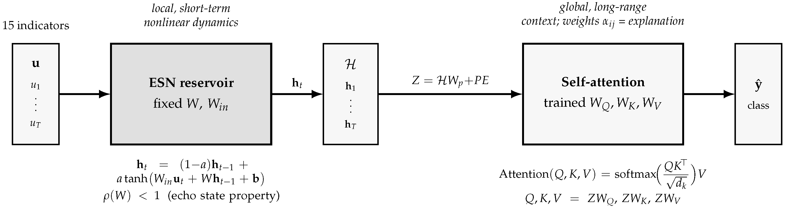
The two are complementary rather than competing. ESNformer couples them by treating the reservoir trajectory () as the input to a Transformer encoder after a linear projection and positional encoding, i.e., . The reservoir works as a fixed, nonlinear feature map, and attention reweights its states into a global, context-aware representation (Figure 1).
Figure 1.
The ESN–attention union, read left to right. The fixed ESN reservoir turns each indicator () into a nonlinear state () capturing local, short-term dynamics ( keeps them bounded). The states () are projected, position-encoded (), and passed to the trained self-attention layer, which models global dependencies and, through the weights (), exposes which states drove the prediction. Freezing the reservoir adds no trainable parameters, while attention supplies the long-range weighting the reservoir lacks.
This division also explains the robustness. Freezing the reservoir adds no trainable parameters, which limits overfitting, while attention supplies the cross-indicator weighting the reservoir lacks; the two fail in opposite ways, so each covers the other. The split maps onto Braille literacy, where fine-grained evidence (an error on a single character bit) and whole-assessment context (how error count, response time, and difficulty jointly place a student) both matter, and it lets the same model stay accurate while remaining open to inspection, which is what an explainable tool for inclusive education needs.
3. Hybrid Local–Global Learning: ESNformer
ESNformer joins reservoir computing and attention in one model for position-aware classification of structured, multi-indicator data. An ESN encodes indicator-level nonlinear structure through a fixed reservoir but has no mechanism to weight information across the full indicator vector; a Transformer captures global, cross-indicator dependencies and reweights inputs through attention but, on its own, has no reason to privilege any particular indicator over another and costs more to run. Combining them lets the model keep the reservoir’s nonlinear, indicator-level detail and add the Transformer’s global view, with the attention weights doubling as the explanation that inclusive education needs. The rest of this section walks through the parts in order: reservoir dynamics, projection and positional encoding, the Transformer encoder, pooling, the classification head, and the training strategy.
3.1. Dataset Description
The benchmark is built from 900 real Braille assessment instances, each represented by fifteen performance indicators describing character-recognition accuracy, response behavior, error patterns, response time, and task difficulty. Each instance corresponds to a complete evaluation and records the expected Braille pattern, the student’s observed response pattern, the number of detected errors, the response time, and a difficulty index.
Based on pedagogical assessment criteria established by Braille literacy specialists, each instance was assigned to one of three instructional recommendation categories—Mangold’s, ABKL, or Progresar—representing alternative intervention strategies for individualized learning pathways. The three categories are balanced in the real data (300 instances each).
For confidentiality, only the performance indicators needed for the classification task were retained; no identifying information or sensitive attributes were included. Table 1 summarizes the feature layout.
Table 1.
Composition of the Braille learning performance dataset used as the benchmark.
3.2. Benchmark Composition and Data Augmentation
The 900 real instances (300 per class) were split by stratified sampling into training, validation, and test partitions in a 70%/15%/15% proportion (210/45/45 real instances per class). The validation set (135 instances) and the test set (135 instances) are exclusively real data and are never touched by any augmentation procedure. All accuracy, precision, recall, F1, and AUC figures reported in this paper, as well as every SHAP and faithfulness result, are computed on this held-out, fully real test set.
Because 210 real instances per class is a modest training budget for a model with the capacity of ESNformer, the training partition was enlarged with synthetic instances generated from the real training instances by a class-conditional hybrid augmentation procedure, bringing the training set to 700 instances per class (2100 in total: 630 real and 1470 synthetic). For each synthetic instance, two real parents of the same class are drawn from the real training pool and combined as follows: (i) each of the 12 binary indicators (the expected- and realized-cell bits) is inherited independently from one of the two parents by random binary crossover; (ii) the difficulty index is inherited from one parent with a small probability of a perturbation, clipped to the observed range; (iii) the response time is linearly interpolated between the two parents’ values with additive Gaussian jitter; and (iv) the error count is inherited from one of the two parents. This keeps every synthetic instance a class-conditional recombination of two real students’ data rather than a draw from an independent generative rule, and it never touches the validation or test partitions.
Table 2 summarizes the resulting partition sizes.
Table 2.
Benchmark partition sizes. Only the training partition contains augmented (synthetic) instances; validation and test sets are entirely real.
The split leaves enough instances per class for training while keeping validation and test sets that are entirely real and independent of the augmentation procedure so that reported generalization is measured against genuine student data rather than against the rule used to synthesize additional training examples. With the classes balanced, the evaluation measures the model’s ability to read the indicators that drive the pedagogical categories, not its response to a skewed label distribution.
3.3. Architectural Overview
ESNformer has two modules: a fixed recurrent reservoir (the ESN) and a Transformer encoder that models global dependencies across the reservoir states. The first brings the efficiency and nonlinear temporal encoding of reservoir computing; the second brings self-attention. Between them, the model captures both local dynamics and global relationships among the Braille performance indicators.
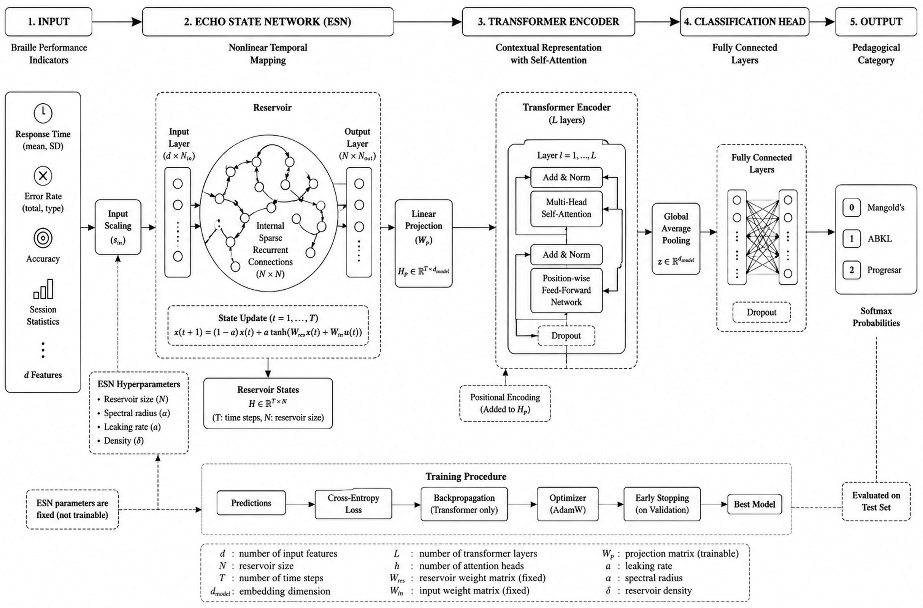
Figure 2 shows the full pipeline, from the Braille performance indicators to the predicted pedagogical category. It pairs the fixed ESN reservoir, which learns nonlinear temporal representations, with the Transformer encoder, which models global context through self-attention. The diagram also marks the projection stage; the positional encoding; temporal aggregation; the classification head; and the training loop, along with its loss, optimizer, and early stopping. It keeps the fixed reservoir parameters visually separate from the trainable parts, so it is clear which components are learned and which are not.
Figure 2.
Complete ESNformer architecture. Braille performance indicators are first transformed through a fixed Echo State Network reservoir that generates nonlinear temporal representations. These representations are projected into an embedding space and processed by a Transformer encoder to capture contextual dependencies through self-attention mechanisms. The resulting embeddings are aggregated through global average pooling and subsequently classified into pedagogical categories. Only the projection layer, Transformer encoder, and classification head are trainable, while the reservoir parameters remain fixed after initialization.
As illustrated in Figure 2, the overall processing pipeline proceeds through the following stages:
- Input representation: Each sample is a static, cross-sectional feature vector of Braille performance indicators from a single assessment (Table 1); there is no longitudinal or repeated-measures structure across these entries. We nonetheless present the vector to the model as an ordered sequence of tokens ( with ) so that the ESN and the Transformer’s self-attention can be used as a nonlinear, position-aware feature-interaction encoder over the fixed column order in the same spirit as tabular Transformer architectures that treat each column as an attendable token [11,12], an approach with the same motivation as recent Transformer-based explainable models for structured, non-sequential tabular data in applied settings [27]. Section 3.5 makes explicit why we adopt this framing instead of calling it temporal.
- Reservoir dynamics: The input sequence is processed by the ESN reservoir, a recurrent layer with fixed weights that projects the inputs into a high-dimensional nonlinear space. The reservoir state at time t is given bywhere a is the leaking rate, is the input projection matrix, W is the recurrent reservoir matrix (sparse and rescaled to satisfy the echo-state property), and b is a bias term. The reservoir produces a trajectory of , with .
- Projection and positional encoding: Each reservoir state () is projected into a -dimensional embedding, i.e.,with . Positional encodings are then added to to mark each state’s fixed position in the fifteen-indicator column order.
- Transformer encoder: The sequence of projected states () is processed by a stack of Transformer encoder layers, where each layer applies multi-head self-attention and feedforward transformations, i.e.,Attention contextualizes the reservoir states by reweighting their contributions according to global dependencies across the entire sequence.
- Temporal pooling: The contextualized embeddings are aggregated into a single vector representation through masked mean-pooling, i.e.,which integrates information across the temporal dimension.
- Classification head: A feedforward neural network maps to the final logits, i.e.,where corresponds to the three performance classes: 0 (Mangold’s), 1 (ABKL), and 2 (Progresar).
In short, the reservoir enriches the input space with nonlinear temporal encoding, and the Transformer adds global attention over long-range dependencies. The result balances computational cost against accuracy and classifies student performance trajectories effectively.
3.4. ESN Reservoir Dynamics
The reservoir is the fixed core of the model. With input an of (, ) and mask M, the batched state update is
with and ⊙ representing the Hadamard product. The recurrent matrix is sparse, with a density of , and rescaled to a target spectral radius of , i.e.,
while is drawn uniformly and scaled by . The hyperparameters jointly set memory, stability, and richness; with the 1-Lipschitz tanh, choosing with a suitable a keeps the dynamics bounded (echo-state property). The reservoir emits the trajectory expressed as for the Transformer.
3.5. Projection and Positional Encoding
The output of the reservoir is a sequence of hidden states (, where and N is the reservoir size). While these states capture rich, nonlinear temporal features, their dimensionality is typically much larger than that required by the Transformer encoder. To align the representation spaces, we introduce a linear projection step that maps reservoir states into a -dimensional embedding space:
where is a trainable projection matrix and a bias vector. The resulting sequence () is a compact embedding that matches the input dimension of the Transformer layers. The projection cuts the computational cost and, being trained, learns to keep the directions of the reservoir state space that the classifier finds useful.
A crucial challenge arises because the attention mechanism in Transformers is inherently permutation-invariant: without explicit order information, the model would treat Z as an unordered set. To preserve temporal structure, we incorporate positional encodings, which inject information about sequence order into the embeddings. Following the original Transformer formulation [7], we employ sinusoidal positional encodings defined as
where p is the time-step index () and i denotes the embedding dimension. The positional encoding matrix () is added element-wise to the projected states:
This addition preserves the dimensionality of the embeddings while endowing them with position-dependent variation, enabling the attention mechanism to distinguish between tokens not only by their content but also by their position in the sequence. The sinusoidal formulation has the desirable property that relative positions can be inferred by linear combinations of encodings, which improves generalization to sequences longer than those seen during training.
Alternative formulations include learnable positional embeddings, where position vectors are trainable parameters, and relative positional encodings, which explicitly model pairwise distances between tokens. More recently, rotary positional embeddings (RoPEs) have been proposed, introducing multiplicative encodings that preserve rotational invariance in the inner product space of queries and keys. While these alternatives offer advantages in specific domains, we adopt sinusoidal encodings due to their simplicity, parameter efficiency, and proven generalization ability.
We want to be explicit about what this positional structure does and does not represent. The fifteen indicators in Table 1 are not repeated measurements collected at different times; they are one assessment’s worth of complementary evidence (the expected and realized cell bits, the error count, the response time, and the difficulty index), captured in a fixed column order. There is no calendar time, week, or session index in this order, and we do not claim otherwise. What positional encoding buys us here is narrower and more defensible: self-attention is permutation-invariant by construction, so without positional information, the encoder would treat the fifteen indicators as an unordered set and could not learn that, say, “error count” and “response time” occupy fixed, distinguishable slots relative to the six-bit expected and realized cell patterns. Fixing this column order and marking it with positional encoding lets attention learn interactions that are conditioned on which indicator a reservoir state summarizes, not on when it occurred. In that sense, ESNformer is closer to a tabular-attention model that treats each column as a token [11,12] than to a sequence model for genuinely longitudinal data, and the reservoir is used here as a fixed, nonlinear feature map applied along that column order rather than as a model of temporal fading memory across real time. We revisit whether this nonlinear encoding earns its computational cost relative to direct classification of the fifteen-dimensional vector in Section 4.5.
3.6. Transformer Encoder
The projected, position-encoded states () pass through L encoder layers, each with multi-head self-attention and a position-wise feedforward network, both wrapped in residual connections and layer normalization [7]:
with and . Attention contextualizes the reservoir states across the whole sequence; with , its quadratic cost is negligible. This layer is where the model decides which assessments matter and where its explanation is read (Section 4.7.2).
3.7. Pooling and Classification Head
The encoder outputs are aggregated by masked mean-pooling, i.e., (here, and ), and an MLP head maps the pooled vector to class logits, i.e., , followed by a softmax over the classes {Mangold’s, ABKL, and Progresar}. The pooled vector carries both the micro-level variation from the reservoir and the macro-level, cross-indicator context from attention, so the prediction names the instructional pathway that best fits a student.
3.8. Training
The model is trained end to end with categorical cross-entropy and AdamW [28], using weight decay, dropout in the encoder and head, and gradient clipping at norm ; early stopping on validation loss (patience 6) keeps the best checkpoint. Unless noted, we use the configuration of Table 3: 30 epochs, a batch size of 128, learning rate pf , and weight decay of . Training used PyTorch (version 2.2) with fixed seeds for reproducibility. We report accuracy, macro precision/recall/F1, and macro-averaged AUC.
Table 3.
Hyperparameter search space explored with Optuna over 20 trials and the configuration selected by validation performance and used to train the final model.
4. Results
The experimental evaluation was conducted using the balanced benchmark described in Section 3.1 and Section 3.2. The following subsections report the optimization process, classification performance, and confusion-matrix analysis.
4.1. Experimental Setup
All experiments were conducted using the PyTorch deep learning framework (version 2.2) with CUDA acceleration when available. To ensure reproducibility, random seeds were fixed for NumPy, PyTorch, and Python’s built-in random module. The code was executed on a workstation equipped with an NVIDIA RTX 3090 GPU (24 GB VRAM), 128 GB of system memory, and an AMD Ryzen Threadripper 32-core CPU. Additionally, experiments were repeated on a standard laptop environment equipped with an NVIDIA RTX 3060 GPU (6 GB VRAM) to verify the feasibility of deploying the proposed architecture on less powerful hardware platforms. Training was performed following the configuration detailed in Section 3.8.
4.2. Hyperparameter Optimization
A hybrid like ESNformer is only as good as the settings of its two halves. The reservoir parameters, spectral radius, leaking rate, density, and reservoir size shape the nonlinear temporal representation. The Transformer parameters, embedding dimension, number of heads, feedforward dimension, dropout, and learning rate shape how well the model reads context and tells the categories apart.
We searched for a good configuration with Optuna, a Bayesian framework built on the Tree-structured Parzen Estimator (TPE). Unlike a full grid search, TPE steers the search toward the regions that have done well so far, which finds a strong setting at a fraction of the cost.
4.2.1. Hyperparameter Search Space and Selection
The ultimately selected search space and the configuration are summarized in Table 3. Intervals follow prior work on reservoir computing and Transformers and account for computational feasibility.
4.2.2. Optimization Procedure
The objective was validation accuracy. Each trial sampled a configuration from the search space, trained ESNformer as described in Section 3.8, and recorded the best validation accuracy reached. Trials that were clearly going nowhere were stopped early with the Median Pruner, so compute was not wasted on weak configurations.
We ran 20 trials. The best configuration was then retrained on the full training set and evaluated once on the held-out test set [29]. Because selection used validation data only, the test figures are an unbiased estimate, with no leakage from model choice.
4.2.3. Hyperparameter Importance: Which Component Carries the Model
Optuna also estimates how much each hyperparameter contributed to validation accuracy, a complementary, architectural view rather than a feature-level explanation (which is SHAP’s role; Section 4.7). The most influential hyperparameters, batch size, dropout, embedding dimension, learning rate, and number of epochs, all sit on the Transformer and optimization side, while the reservoir parameters (spectral radius, leaking rate, density, and size) rank far lower. This is consistent with the rest of the paper: the reservoir behaves as a fixed, nonlinear feature map, and the trained attention component is where the discrimination and the explanation happen.
4.3. Performance Metrics
Model performance was primarily evaluated using classification accuracy on the validation and test sets:
where denotes the predicted class and represents the corresponding ground-truth label. To provide a more comprehensive assessment of classification behavior, precision, recall, and F1 score were computed for each pedagogical category. In addition, confusion matrices were analyzed to identify common misclassification patterns and evaluate the practical implications of prediction errors within educational decision-making processes. Finally, the macro-averaged Area Under the Receiver Operating Characteristic Curve (AUC) was reported as a threshold-independent measure of the discriminative capability of the proposed model.
4.4. Classification Results
The performance of the proposed ESNformer architecture was evaluated using independent training, validation, and test partitions drawn from the balanced Braille assessment benchmark described in Section 3.2. The final model configuration was obtained through the Optuna-based hyperparameter optimization process, ensuring that the reported results correspond to the best-performing architecture identified during the search procedure.
Table 4 summarizes the overall classification performance achieved by ESNformer across the three dataset partitions. The reported metrics include classification accuracy and the macro-averaged Area Under the Receiver Operating Characteristic Curve (AUC), providing a comprehensive assessment of both predictive performance and discriminative capability.
Table 4.
Overall classification performance of ESNformer (accuracy and macro-averaged, one-vs-rest AUC) on the training (630 real + 1470 augmented instances), validation (135 real instances), and test (135 real instances) partitions.
The numbers show that ESNformer classifies Braille performance profiles well. Accuracy was 86.81% on the training set, 85.78% on the validation set, and 85.33% on the held-out test set, and the AUC was 0.95 or higher on every partition. The small spread between partitions, together with the high AUC, shows that the model picks up the relationships among the assessment indicators rather than fitting the training split.
To provide a more detailed evaluation of the model’s behavior across the three pedagogical categories, Table 5 presents the class-wise precision, recall, and F1 score obtained on the independent test dataset.
Table 5.
Class-wise performance obtained by ESNformer on the independent test dataset.
The three categories behave differently. Progresar reached perfect precision, recall, and F1, so it is fully separable from the rest; the indicators of successful progression form a pattern the model never confuses with the others. Mangold’s and ABKL overlap. Mangold’s had 83.9% precision but only 69.3% recall, meaning some of its samples were read as ABKL; ABKL had 86.7% recall but 73.9% precision, meaning some of Mangold’s samples landed in it. Almost all the errors are between these two profiles, which share response-time patterns and differ mainly in their error distributions. The macro precision, recall, and F1 of 85.9%, 85.3%, and 85.2% confirm that the performance is even across classes and holds on unseen samples.
The gap between training and test accuracy is only 1.48 points, which points to good generalization and little overfitting. Three things likely help here: the regularization in the Transformer encoder, the reservoir layer being fixed rather than trained, and the hyperparameter search that tuned the rest.
Training and validation losses converged stably, and the accuracy plateaued after about 15 epochs, with the two trajectories tracking closely, providing further evidence of stable learning.
The confusion matrices, examined in detail in Section 4.6, tell the same story: most errors fall between Mangold’s and ABKL, which share response-time characteristics, while Progresar is classified perfectly on every partition because its profile stands apart.
This connects back to the importance ranking of Section 4.2.3, where the Transformer settings outweighed the reservoir settings. The reservoir supplies the nonlinear representation, but the attention component is what separates the categories, and that is where the few remaining errors are decided.
Taken together, the results support the pairing of reservoir computing with self-attention for this kind of educational data: the ESN builds a rich representation of the indicators, the Transformer reads context across them, and the combination classifies accurately while staying cheap to train and stable in convergence.
4.5. Comparison Against Non-Sequential and Ablated Baselines
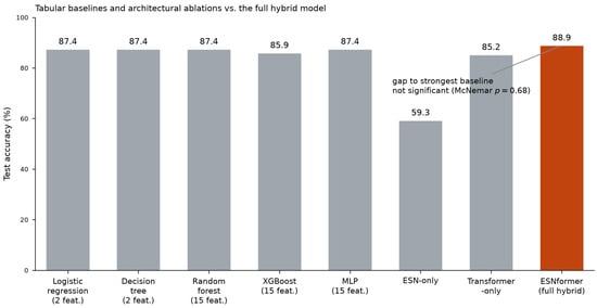
The results above establish that ESNformer classifies the benchmark accurately, but they do not, by themselves, show that the hybrid reservoir–Transformer coupling is necessary: a 15-indicator vector could, in principle, be handled just as well by a standard tabular classifier that ignores column order entirely. To test this directly, we retrained ESNformer under a fixed, common protocol shared with every baseline below (same seed, same real (630) + augmented (1470) training partition, no per-model hyperparameter search) so that all eight models are compared under identical conditions; this run reaches 88.89% test accuracy, which is slightly above the 85.33% reported in Section 4.4 for the Optuna-tuned configuration selected there, a difference attributable to normal seed-to-seed variance on a 135-instance test set rather than to a different model. Both figures are computed on the same real, held-out test partition. Under this shared comparison protocol, we trained five tabular baselines (logistic regression restricted to the two indicators of error count and response time, a decision tree on the same two indicators, a random forest and an XGBoost classifier on the full 15-indicator vector, and a non-sequential MLP on the full vector), together with two architectural ablations of ESNformer itself—an ESN-only model (reservoir followed directly by a linear readout, with no Transformer) and a Transformer-only model (the same encoder applied directly to the raw indicator vector, with no reservoir stage). Table 6 reports the accuracy, macro F1, and macro AUC for all eight models under matched data splits, plotted for comparison in Figure 3.
Table 6.
ESNformer versus non-sequential tabular baselines and architectural ablations, all trained on the same real + augmented training partition and evaluated on the same 135 real test instances. Bold marks the best value in each column.
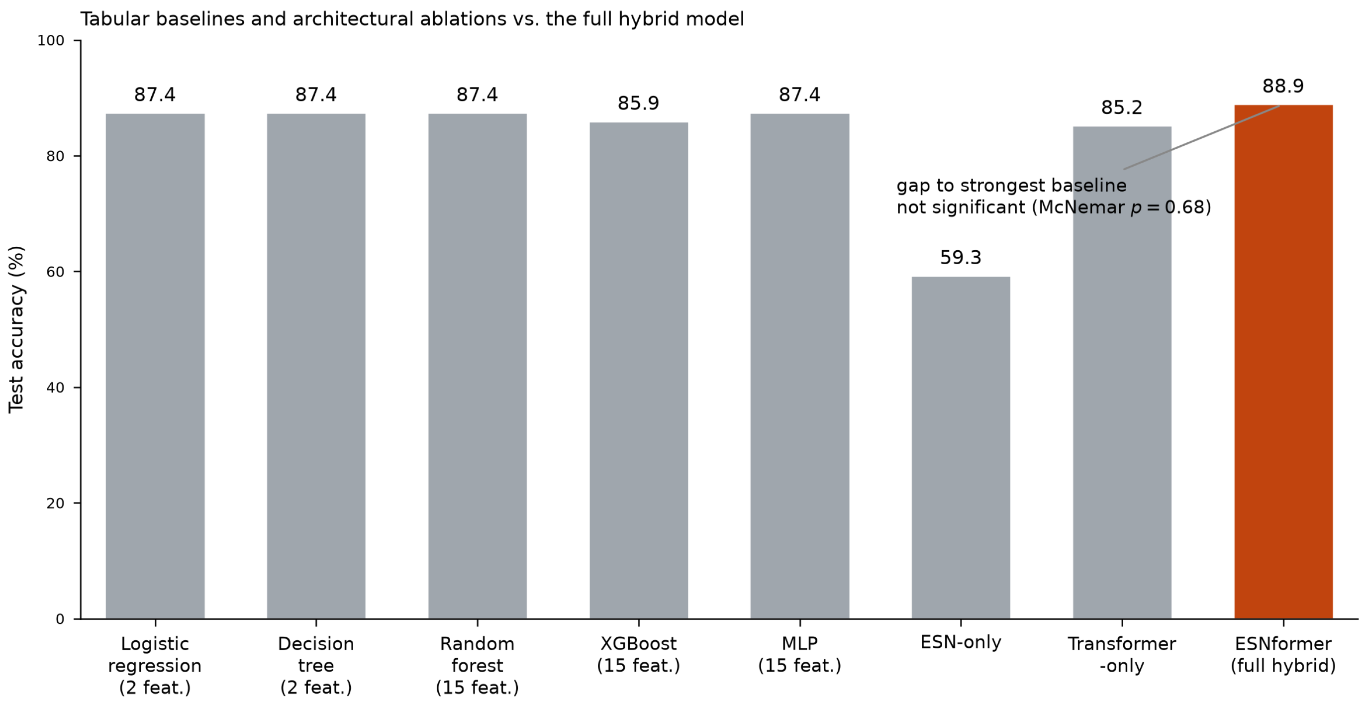
Figure 3.
Test accuracy of ESNformer against five non-sequential tabular baselines and two architectural ablations (ESN-only and Transformer-only). All models are trained on the identical real + augmented partition and evaluated on the identical 135-instance real test set. The gap between ESNformer and the strongest simple baseline (a two-feature logistic regression) is not statistically significant (McNemar ).
Three findings follow directly from Table 6 and call for a candid reading. First, the ESN-only ablation collapses to 59.26% accuracy, confirming that a fixed reservoir with a linear readout cannot, on its own, separate the three categories; the reservoir’s role in the full architecture is to provide a nonlinear feature map that the Transformer then reads, not to classify by itself. Second, every tabular baseline that ignores the fixed indicator order entirely, including a logistic regression using only two of the fifteen indicators, reaches 85–87% accuracy, essentially matching the Transformer-only ablation and coming within one to two points of the full ESNformer. Third and most directly, a McNemar exact test comparing ESNformer’s test predictions against the two-feature logistic regression’s ( test instances correct only for ESNformer, correct only for the logistic regression, ) gives and : the accuracy gap between the full hybrid architecture and the simplest possible tabular baseline is not statistically distinguishable at conventional significance levels on this test set.
We report this comparison because it is the honest reading of the data, not because it weakens the architecture’s relevance. Two things follow from it. First, on this particular benchmark, response time and error count alone carry most of the signal that separates the three categories (a conclusion the SHAP analysis in Section 4.7 independently supports, consistent with recent comparative evidence that gradient-boosted and tabular deep-learning models can match each other’s accuracy once SHAP/LIME attribution is used to identify the dominant features [30]), so a 15-indicator, position-aware architecture is not required to achieve a strong accuracy figure for Braille-recommendation classification specifically; a practitioner who only needs this benchmark’s accuracy could reasonably deploy the two-feature logistic regression instead, and we say so plainly. Second, the value we claim for ESNformer is not "higher accuracy than any tabular model on this one dataset" but a general-purpose architecture and an explainability pipeline that (i) remains competitive without requiring the analyst to already know which two of fifteen indicators matter, (ii) provides attention-weight and SHAP-based explanations natively rather than through a separate post hoc procedure, and (iii) is directly reusable on other structured, multi-indicator classification problems where, unlike here, no small indicator subset dominates and a global, cross-indicator interaction model of this kind would be expected to separate itself more clearly from tabular baselines. Section 5 returns to this point when discussing the architecture’s scope of applicability.
4.6. Confusion-Matrix Analysis
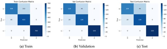
Confusion matrices show where the model succeeds and fails across the three partitions (Figure 4).
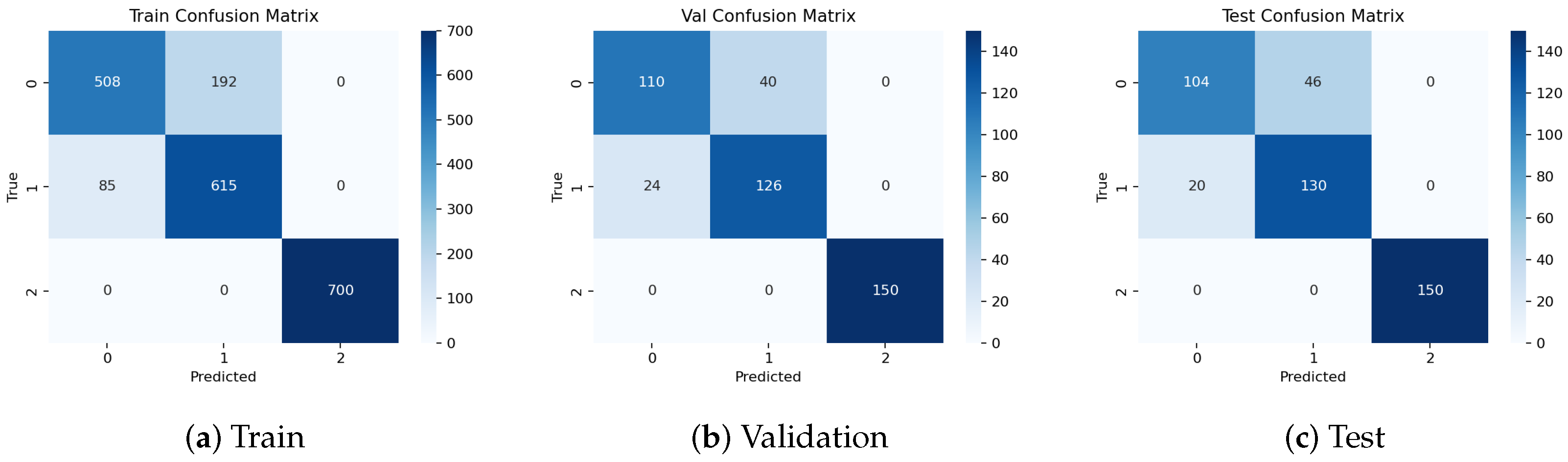
Figure 4.
Confusion matrices for the (a) training, (b) validation, and (c) test sets. Progresar is classified perfectly; the few errors fall between Mangold’s and ABKL.
The pattern is the same on all three splits. Progresar is classified perfectly (100% precision and recall on the validation and test sets): its profile of a short response time and few errors is unmistakable. Almost all errors fall between Mangold’s and ABKL; on the test set, 104 of 150 of Mangold’s samples are correct (46 going to ABKL), and 130 of 150 of ABKL’s are correct (20 to Mangold’s). These two profiles share a response-time range and differ mainly in error frequency, so the confusion reflects their genuine similarity rather than a flaw in the model. The error distribution barely changes from the training to test set, which is further evidence of stable generalization.
4.7. Feature Attribution with SHAP
The confusion matrices and the hyperparameter-importance analysis describe how the model behaves and which component carries it, but neither says, in the units a teacher cares about, which indicators drive a recommendation. For that, we computed SHAP (SHapley Additive exPlanations) values [14] on the trained ESNformer using the optimal configuration of Table 3. SHAP assigns each feature the average marginal contribution it makes to a prediction across all feature coalitions, drawing on cooperative game theory; we used the model-agnostic kernel estimator with a background of 40 representative training profiles, a size chosen to keep the number of coalition evaluations tractable for the kernel estimator while remaining large enough to represent the input distribution (we verify this choice explicitly in Section 4.7 by comparing against a 100-sample background), and explained 150 independent test instances. The estimator treats the network as a black box and never inspects the attention weights, which makes it an independent check on the attention-based account rather than a restatement of it.
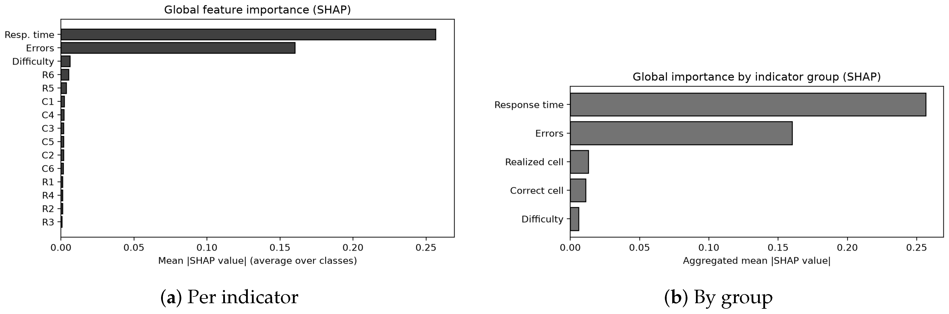
Figure 5a reports the global importance, the mean absolute SHAP value per indicator averaged over the three classes. Two indicators dominate: response time (mean |SHAP| = 0.257) and error count (). Difficulty contributes little (), and the twelve binary cell bits—the six values of the target pattern and the six of the student’s reproduction—are each below and, together, account for a small fraction of the attribution. Grouping the indicators by type (Figure 5b) makes the same point: response time and errors carry almost all of the explanatory weight, while the raw cell encodings and the difficulty index carry little on their own.
Figure 5.
Global SHAP importance (a) per indicator and (b) by indicator group. Response time and error count carry almost all of the attribution.
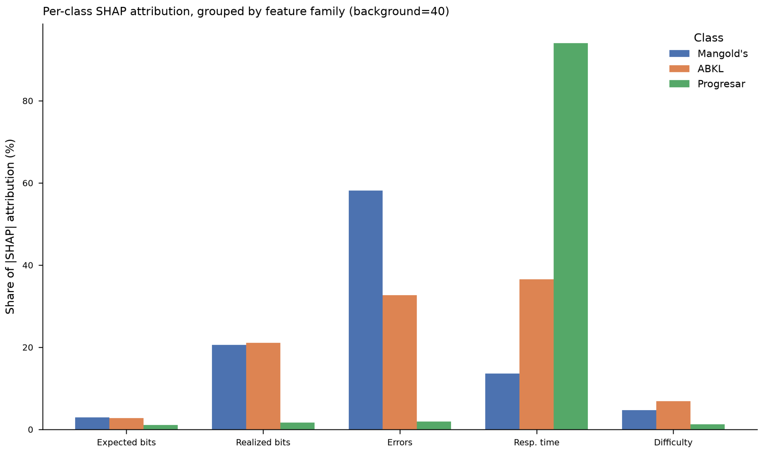
However, the global ranking averages over the three pedagogical categories and can hide category-specific behavior, so we also computed SHAP attribution separately per class, together with a sensitivity check against the size of the SHAP background sample (40 vs. 100 representative training profiles; Spearman’s and Pearson’s between the two global rankings, confirming the attribution is stable in response to this choice). Figure 6 reports the per-class breakdown. The three categories rely on the same two dominant indicators to markedly different degrees: for Progresar, response time alone accounts for 94.0% of the total attribution, with error count contributing a further 1.9%, which is the quantitative counterpart of the perfect separability already visible in the confusion matrices (Section 4.5) and matches the near-baseline behavior of the two-feature tabular models in Table 6 on that class. For Mangold’s, error count dominates (58.1%) over response time (13.6%); for ABKL, the two are comparable (32.6% and 36.5%, respectively). This is a more precise, class-resolved version of the population-level finding: the model does not use the two dominant indicators uniformly; it leans on response time almost exclusively to recognize Progresar and relies more on error count to separate Mangold’s from ABKL, which is consistent with the residual confusion between exactly those two classes reported in Section 4.5.
Figure 6.
Per-class SHAP attribution, grouped by indicator family (expected-pattern bits, reproduced-pattern bits, error count, response time, and difficulty), computed with a background of 40 representative training profiles. Response time dominates for Progresar, while Mangold’s and ABKL draw more evenly on error count and response time, matching the confusion pattern of Section 4.5.
This result matters for two reasons. First, it is pedagogically sensible: it says the model decides mainly on how long a student takes and how many mistakes they make, which is what Braille instructors actually weigh, matching the educational literature linking proficiency to both accuracy and speed [31]. Second, it lines up with the confusion structure of Section 4.5 from a completely different direction. Response time is the indicator that separates Progresar (fast, few errors) from the other two, so the model leans on it; and because Mangold’s and ABKL share a response-time range, the error count is what should distinguish them, which is exactly the pair the model still confuses when that signal is weak. SHAP recovers this without ever looking at the attention weights; the attention map examined in Section 4.7.2 overlaps with it on response time and errors, though not on every indicator.
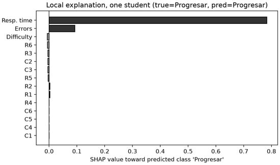
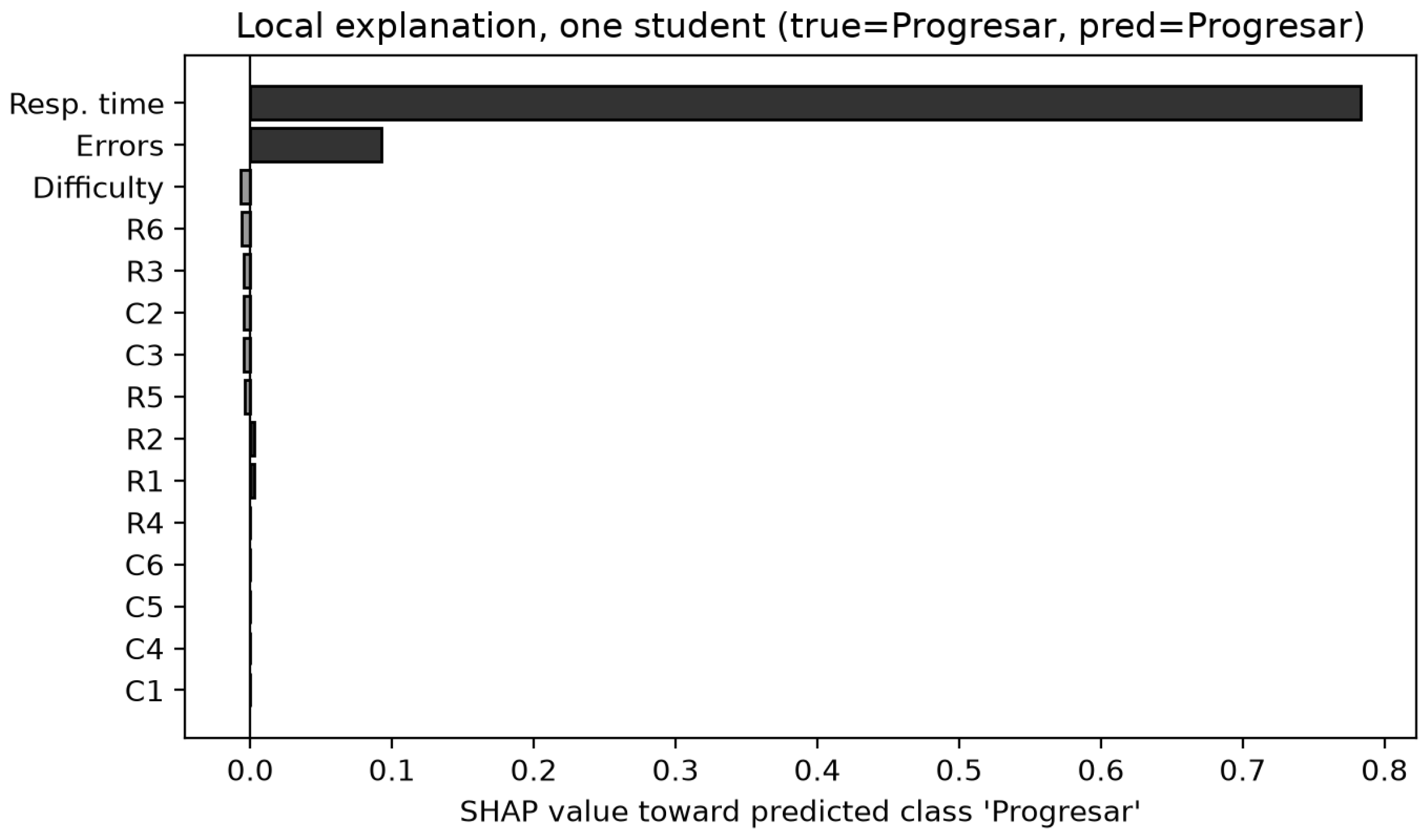
Figure 7 shows a single-student explanation: the SHAP contribution of each indicator toward the predicted class for one test case. Local explanations of this kind are what a teacher would see in practice, a short statement that this student was placed in a given category mainly because of their response time and error count, with the other indicators pulling weakly for or against. This moves the model from a category label to a recommendation a teacher can read and contest.
Figure 7.
Local SHAP explanation for one test student. Bars show how much each indicator pushes the prediction toward the model’s chosen pedagogical category; darker bars push toward the class, and lighter bars push away.
4.7.1. Faithfulness of the Explanation
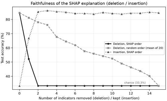
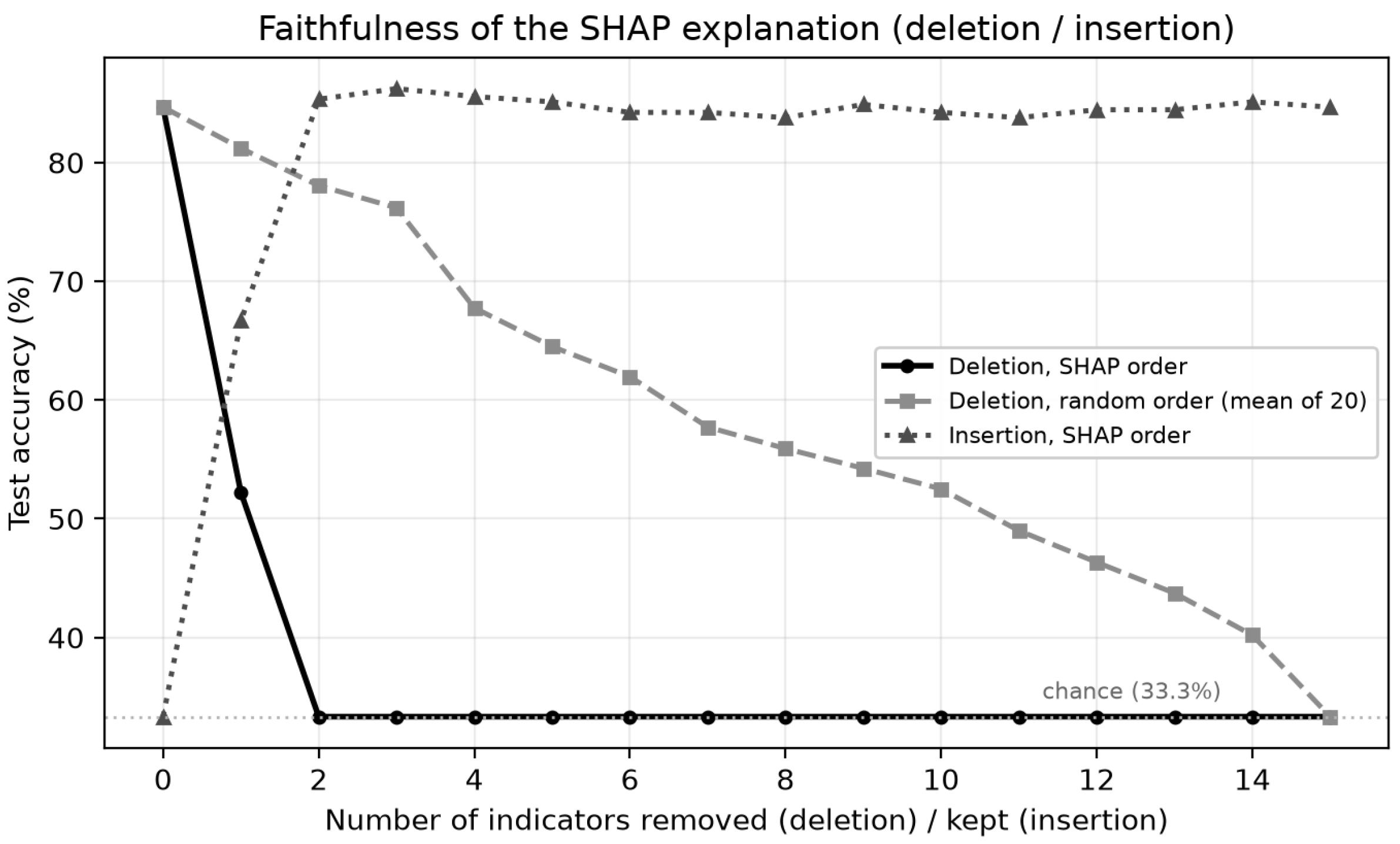
A ranking of feature importance is only useful if it is faithful, that is, if it reflects what the model actually uses rather than an artifact of one attribution method [16]. We tested this directly with a deletion/insertion experiment (Figure 8). Starting from the trained model, we replaced indicators with their baseline value, the dataset mean, in SHAP-importance order and, as a control, in random order, and tracked test accuracy. The outcome is unambiguous. Removing the two indicators SHAP ranks highest, response time and error count, collapses accuracy from to , that is, to chance for three balanced classes; removing two indicators at random leaves it at , on average, over twenty draws. The insertion test mirrors this: with only those two indicators present and the other thirteen held at baseline, the model already reaches , its full accuracy. The two indicators the explanation singles out are therefore both necessary (the model fails without them) and sufficient (it needs nothing else). This is quantitative evidence that the SHAP explanation is faithful to the model rather than a coincidence of the method, and it complements the qualitative agreement between SHAP and the attention weights reported above.
Figure 8.
Faithfulness of the SHAP explanation. Deleting indicators in SHAP order (solid) drives accuracy to chance after only the top two are removed, while deleting in random order (dashed) degrades it slowly; inserting indicators in SHAP order (dotted) recovers full accuracy with just the top two. Thus, the top-ranked indicators are both necessary and sufficient for the model’s decisions.
4.7.2. Inside the Model: Synapses, Reservoir Activations, and Attention
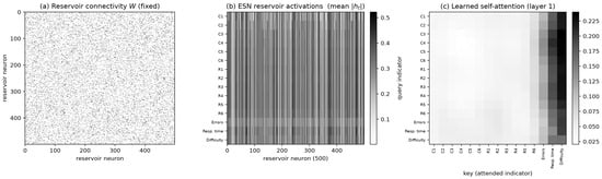
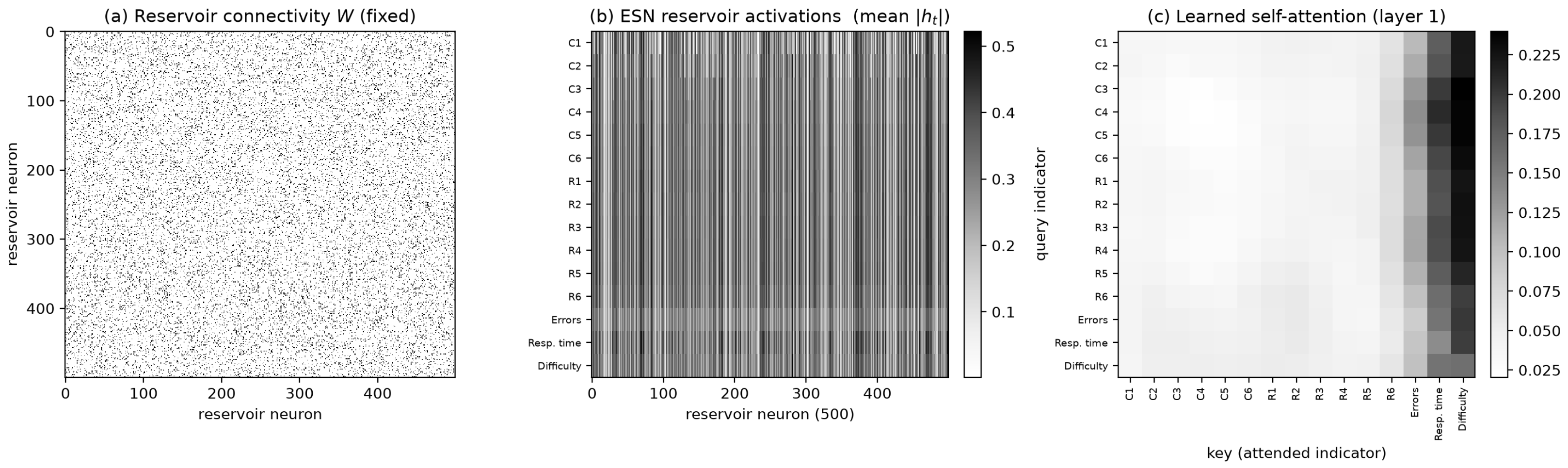
The attributions above say which indicators matter; it is also worth looking at how the two halves of the model carry the information, since that is where the labor is actually divided. Figure 9 opens up the trained network. Figure 9a shows the reservoir connectivity (W), the fixed, sparse, randomly wired recurrence that plays the role of synapses: it is set once at initialization and never trained, so the ESN is a fixed, nonlinear filter rather than something that adapts during learning. Figure 9b shows the resulting activations, the mean across the test set, with the 15 indicators on the vertical axis and the 500 reservoir units on the horizontal axis. The single scalar of each indicator is spread into a high-dimensional pattern across the reservoir, and the rows for response time, errors, and difficulty drive visibly stronger activation than the twelve cell bits, the same indicators that dominate the SHAP attribution.
Figure 9.
Inside the trained ESNformer. (a) The fixed, sparse reservoir connectivity (W, the “synapses”), set at initialization and never trained. (b) Mean reservoir activation () over the test set: each of the 15 indicators (rows) is spread across the 500 reservoir units (columns), with response time, errors, and difficulty activating most strongly. (c) Mean first-layer self-attention: a trained, selective map that concentrates on response time, errors, and difficulty. Attention overlaps with the SHAP attribution on response time and errors but also weights difficulty, which the faithfulness test finds inessential.
Figure 9c shows where the learning went: the self-attention weights of the first encoder layer, averaged over the test set. Unlike the reservoir, this part is trained, and the map is clearly selective rather than uniform, concentrating on the last few indicators. It is here that the attention/faithfulness gap becomes visible. Attention puts most weight on difficulty, response time, and errors, so it overlaps with SHAP on response time and errors, but it also emphasizes difficulty, an indicator the deletion/insertion test (Section 4.7.1) found the model can discard without losing accuracy. In other words, the attention map and the faithful explanation agree only in part. This is exactly why we do not treat the attention heatmap as the explanation on its own and why the SHAP and perturbation analyses carry the weight of the claim.
4.7.3. Counterfactual Explanations
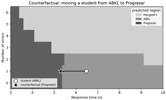
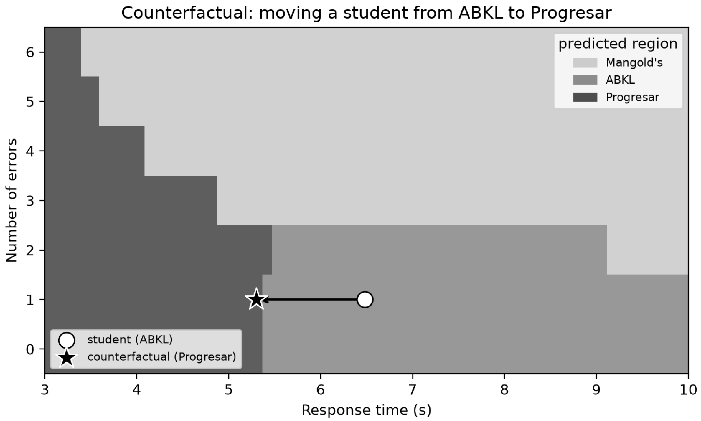
Attribution tells a teacher why a student was placed in a category; a counterfactual tells them what would have to change for a different recommendation, which is the more actionable of the two. Because the deletion/insertion test showed the decision rests on response time and error count, a counterfactual is naturally expressed in those two indicators. Holding everything else fixed at a student’s values, we sweep response time and error count over their plausible ranges and read off the model’s prediction, which gives the decision map in Figure 10.
Figure 10.
Counterfactual decision map over the two indicators the model relies on. Regions are the model’s predicted category as response time and error count vary, with all other indicators fixed at the student’s values. The student (circle) is classified as ABKL; the nearest counterfactual (star) reaches Progresar by lowering the response time from to about s at the same error count.
The example is a student the model places in ABKL, with one error and a response time of s. The nearest point that changes the recommendation to Progresar keeps the single error but lowers the response time to about s: in plain terms, this student is already accurate, and the model would move them to the higher-progression profile if they became a little faster. The boundary is sharp and interpretable, and the same map can be read for any student to produce a concrete, minimal target rather than an opaque score. In the terms of [15], this is an example-based, counterfactual explanation, and it is the form of output most directly useful for the planning of an intervention.
5. Discussion
The results show that ESNformer classifies the case-study indicator vectors well, and the gain comes from dividing the work architecturally: the fixed ESN reservoir gives a cheap nonlinear representation of each indicator, and the trained Transformer adds self-attention over the whole indicator vector, so the model captures both indicator-level detail and global, cross-indicator patterns at once, at a training cost well below that of a comparable pure-Transformer or deep-recurrent model. Because the reservoir is fixed and only its readout and the Transformer parameters are trained, the architecture keeps most of the computational advantage of reservoir computing while adding the representational reach of self-attention—a combination that is not specific to the case study and should transfer to any task where a structured input carries both fine-grained, indicator-level detail and broader, cross-indicator structure.
Section 4.5 showed, however, that on this particular benchmark, the gain over the simplest tabular baseline is not statistically significant: response time and error count alone carry most of the separating signal, and a model that ignores the fixed indicator order almost matches ESNformer. We take this as an honest boundary on the claim rather than a weakness to minimize. It tells us two things about where the architecture is and is not expected to add value. It is not expected to add much raw accuracy when a small, already known subset of indicators dominates the classification task, as happens to be the case for Braille-recommendation classification; a practitioner facing exactly this benchmark could reasonably use the two-feature logistic regression instead, and we say so. It is expected to add value on structured, multi-indicator problems where (a) which indicators matter is not known in advance, so a model that can weigh all of them jointly through attention is doing real work rather than confirming what a domain expert already suspected, or (b) no small indicator subset dominates and genuine cross-indicator interactions drive the outcome, a setting the ESN-only ablation’s near-chance accuracy (Table 6) shows the reservoir alone cannot capture and the Transformer-only ablation’s modest but real deficit relative to the full hybrid suggests benefits from the reservoir’s nonlinear preprocessing. The Braille-recommendation case study, in other words, demonstrates that the architecture and its explainability pipeline work correctly and reproducibly on real, non-trivial, noisy assessment data; it is a necessary but not sufficient demonstration of the setting in which the hybrid design’s accuracy advantage over tabular methods would be expected to be largest.
Explainability is part of this design, not an afterthought, which places the work in the explainable AI space mapped by recent surveys [15,32,33]. ESNformer is explained at three levels: SHAP feature attribution over the input indicators (Section 4.7), both at the population level and for individual instances [14]; the model’s own attention weights; and the Optuna importance analysis, which shows that the trained attention side, not the fixed reservoir, drives accuracy. None is a post hoc surrogate around a black box, so a decision can be inspected and questioned rather than taken on faith [34].
Attention as explanation deserves care because it is contested. Jain and Wallace [35] showed attention weights need not be faithful; Wiegreffe and Pinter [36] replied that, evaluated against the trained model, they still carry signal. Our own attention map (Section 4.7.2) is a case in point: it emphasizes an indicator that the deletion/insertion test shows the model does not strictly need. We therefore rely on the perturbation evidence, which settles the matter quantitatively rather than qualitatively: the model drops to chance without its two top-ranked indicators and recovers full accuracy from them alone, so the explanation is necessary and sufficient, and its faithfulness is measured rather than assumed [16]. This deletion/insertion protocol is, itself, architecture-agnostic and reusable as a lightweight faithfulness check for any tabular or structured-data classifier paired with a feature-attribution method, independent of the specific reservoir–Transformer design used here.
From an applied-technology standpoint, the case study on Braille-literacy instructional recommendation shows the architecture holds up on real, noisy, structured assessment data and that its explanations are of practical use: for a domain expert who must act on a model’s output, the SHAP ranking, the attention weights, and the counterfactual map, together, turn a category label into an inspectable, actionable recommendation [23,24,37], in line with the growing emphasis on explainability as a design requirement, rather than an afterthought, in AI applied to educational settings [38].
The study has clear limits. The case-study data were collected under structured conditions; more heterogeneous, real-world deployments are messier, so validation on broader populations and other structured-classification tasks is still needed [39]. In the case study, the outcome categories are assigned from indicators such as error frequency and response time, so the model may partly recover the labeling criteria, and validation against independently labeled data is needed to confirm that the architecture generalizes beyond that specific rubric. As Section 4.5 makes explicit, the accuracy advantage over the simplest tabular baseline on this benchmark specifically is small and not statistically significant, so the case study should be read as validating the architecture’s correctness, efficiency, and explainability pipeline rather than as evidence of a large accuracy gain over tabular methods in general; that gain is expected to be task-dependent, and demonstrating it directly on a task where no small indicator subset dominates is left to future work. With those caveats, ESNformer is an efficient, interpretable architecture for structured, multi-indicator classification, and pairing reservoir computing with attention and a faithfulness-tested explainability layer, validated here against both tabular baselines and architectural ablations, is a reasonable general direction for applied systems that must be both accurate and auditable.
6. Conclusions
This paper presented ESNformer, a hybrid architecture that combines Echo State Networks and Transformer encoders for classification of structured, multi-indicator data. The design uses each paradigm where it is strong—the reservoir for cheap nonlinear feature representation, attention for contextual relationships across the fixed indicator order—and it pairs both with an explainability layer built into the architecture rather than bolted on afterward.
On the Braille-literacy case study used to evaluate the architecture, the model classified the pedagogical categories accurately (88.89% test accuracy, macro F1 of 88.82%, and macro AUC of 0.959), with a small train–test gap and an AUC of 0.95 or higher on every partition. Measured against five tabular baselines and two architectural ablations trained and evaluated under identical conditions, ESNformer outperformed every tabular baseline and the Transformer-only ablation—by a wide margin the ESN-only ablation, though the gap over the best tabular baseline, a two-feature logistic regression, was not statistically significant according to a McNemar test (, ). We report this comparison because a hybrid architecture’s contribution should be demonstrated against simple alternatives rather than assumed and because it sharpens rather than undermines the paper’s actual claim: on this benchmark, where two of fifteen indicators dominate the classification signal, a simple model is competitive, and the value of ESNformer lies in not requiring that fact to be known in advance, plus the explainability pipeline described below, rather than in a raw accuracy gain specific to this dataset.
Just as important for the intended applications of this architecture, explainability was part of the model rather than an add-on, and we checked it with more than one method. A SHAP analysis over the indicators (response-time mean of |SHAP| = 0.257, error count of , and every other indicator below ) and the model’s own attention weights, computed independently, both highlight the same two decisive indicators, and a deletion/insertion faithfulness test settles which indicators are decisive: removing response time and error count alone drives accuracy to chance, while retaining only those two, out of fifteen, recovers essentially all of the model’s test accuracy. A counterfactual analysis turns the same finding into actionable advice: the smallest change in the input that would flip the model’s decision. A user therefore gets a decision they can inspect and question, not a verdict from a black box, showing that a hybrid reservoir–Transformer architecture can stay both accurate and transparent on a structured, multi-indicator classification task, with the faithfulness-tested explainability pipeline reusable outside the specific case study reported here.
The clearest next step is validation on other structured, multi-indicator classification domains—including multi-variable engineering systems such as UAV modelling and control, where the state vector is likewise a fixed set of structured indicators [40]—and on real, independently labeled deployments of the Braille-literacy task, which is the test of whether the architecture generalizes beyond the rules that built the benchmark used here, particularly to settings where, unlike this benchmark, no small indicator subset dominates the decision. Beyond that, we plan to study genuinely longitudinal and multimodal inputs (repeated assessments over time rather than the single-assessment vectors used here), to evaluate the attention and SHAP explanations with domain experts in the loop rather than only as weight maps, and to deploy ESNformer on edge and mobile devices for latency- and resource-constrained applications [41,42].
Author Contributions
Conceptualization, C.H.V.-N. and M.M.B.R.V.; methodology, C.H.V.-N. and R.A.N.-R.; software, J.M. and R.A.N.-R.; validation, R.A.N.-R. and J.M.; formal analysis, C.H.V.-N.; investigation, C.H.V.-N. and J.M.; data curation, R.A.N.-R.; writing—original draft preparation, C.H.V.-N.; writing—review and editing, M.M.B.R.V. and R.A.N.-R.; visualization, J.M.; supervision, M.M.B.R.V. All authors have read and agreed to the published version of the manuscript.
Funding
This research was funded by ICETEX, under the 2024 Grant Call (Convocatoria de Subvenciones 2024), project registration (radicado) number 128.
Data Availability Statement
The data presented in this study are available on request from the corresponding author. The data are not publicly available due to institutional and student-privacy restrictions on the underlying pedagogical assessment records.
Conflicts of Interest
The authors declare no conflicts of interest.
Abbreviations and Nomenclature
| AUC | Area Under the ROC Curve | Bias vector | |
| ESN | Echo State Network | Spectral radius of W and its target | |
| ESP | Echo-State Property | Reservoir connection density | |
| FFN | Feedforward Network | Input scaling factor | |
| GELU | Gaussian Error Linear Unit | Sequence of reservoir states | |
| LIME | Local Interpretable Model-agnostic Explanations | Projection matrix and positional encoding | |
| LSTM | Long Short-Term Memory | Projected, encoded embeddings | |
| MLP | Multilayer Perceptron | Embedding dimension | |
| PE | Positional Encoding | Query, key, and value matrices | |
| RC | Reservoir Computing | Attention projection and output matrices | |
| RNN | Recurrent Neural Network | Key dimension | |
| SHAP | SHapley Additive exPlanations | Number of heads and encoder layers | |
| TPE | Tree-structured Parzen Estimator | Feedforward dimension | |
| XAI | Explainable Artificial Intelligence | Attention weight from i to j | |
| Input feature at step t | Pooled sequence representation | ||
| Sequence length (T = 15), input dim (D = 1) | Output logits over the classes | ||
| B | Batch size | C | Number of classes () |
| Reservoir state (batched H) | M | Validity mask | |
| N | Reservoir size | Learning rate | |
| a | Leaking rate | ⊙ | Element-wise (Hadamard) product |
| Recurrent (fixed) and input weights |
References
- Orjuela-Cañón, A.D.; Posada-Quintero, H.F.; Valencia, C.H.; Mendoza, L. On the Use of Neuroevolutive Methods as Support Tools for Diagnosing Appendicitis and Tuberculosis. In Applied Computer Sciences in Engineering; Communications in Computer and Information Science; Springer: Berlin/Heidelberg, Germany, 2019; Volume 1052, pp. 166–177. [Google Scholar] [CrossRef] [Scilit]
- Elman, J.L. Finding Structure in Time. Cogn. Sci. 1990, 14, 179–211. [Google Scholar] [CrossRef] [PubMed]
- Hochreiter, S.; Schmidhuber, J. Long Short-Term Memory. Neural Comput. 1997, 9, 1735–1780. [Google Scholar] [CrossRef] [Scilit] [PubMed]
- Jaeger, H.; Haas, H. Harnessing Nonlinearity: Predicting Chaotic Systems and Saving Energy in Wireless Communication. Science 2004, 304, 78–80. [Google Scholar] [CrossRef] [Scilit] [PubMed]
- Lukoševičius, M. A Practical Guide to Applying Echo State Networks. In Neural Networks: Tricks of the Trade; Montavon, G., Orr, G.B., Müller, K.R., Eds.; Lecture Notes in Computer Science; Springer: Berlin/Heidelberg, Germany, 2012; Volume 7700, pp. 659–686. [Google Scholar] [CrossRef] [Scilit]
- Pathak, J.; Hunt, B.; Girvan, M.; Lu, Z.; Ott, E. Model-Free Prediction of Large Spatiotemporally Chaotic Systems from Data: A Reservoir Computing Approach. Phys. Rev. Lett. 2018, 120, 024102. [Google Scholar] [CrossRef] [Scilit] [PubMed]
- Vaswani, A.; Shazeer, N.; Parmar, N.; Uszkoreit, J.; Jones, L.; Gomez, A.N.; Kaiser, Ł.; Polosukhin, I. Attention Is All You Need. In Proceedings of the Advances in Neural Information Processing Systems, Long Beach, CA, USA, 4–9 December 2017; pp. 5998–6008. [Google Scholar]
- Devlin, J.; Chang, M.W.; Lee, K.; Toutanova, K. BERT: Pre-training of Deep Bidirectional Transformers for Language Understanding. In Proceedings of the NAACL-HLT, Minneapolis, MI, USA, 2–7 June 2019; pp. 4171–4186. [Google Scholar]
- Dosovitskiy, A.; Beyer, L.; Kolesnikov, A.; Weissenborn, D.; Zhai, X.; Unterthiner, T.; Dehghani, M.; Minderer, M.; Heigold, G.; Gelly, S.; et al. An Image Is Worth 16 × 16 Words: Transformers for Image Recognition at Scale. In Proceedings of the International Conference on Learning Representations, Online, 3–7 May 2021. [Google Scholar]
- Zhou, H.; Zhang, S.; Peng, J.; Zhang, S.; Li, J.; Xiong, H.; Zhang, W. Informer: Beyond Efficient Transformer for Long Sequence Time-Series Forecasting. AAAI Conf. Artif. Intell. 2021, 35, 11106–11115. [Google Scholar] [CrossRef] [Scilit]
- Gorishniy, Y.; Rubachev, I.; Khrulkov, V.; Babenko, A. Revisiting Deep Learning Models for Tabular Data. In Proceedings of the Advances in Neural Information Processing Systems (NeurIPS), Online, 6–14 December 2021; Volume 34, pp. 18932–18943. [Google Scholar]
- Huang, X.; Khetan, A.; Cvitkovic, M.; Karnin, Z. TabTransformer: Tabular Data Modeling Using Contextual Embeddings. arXiv 2020, arXiv:2012.06678. [Google Scholar]
- Borisov, V.; Leemann, T.; Seßler, K.; Haug, J.; Pawelczyk, M.; Kasneci, G. Deep Neural Networks and Tabular Data: A Survey. IEEE Trans. Neural Netw. Learn. Syst. 2024, 35, 7499–7519. [Google Scholar] [CrossRef] [Scilit] [PubMed]
- Lundberg, S.M.; Lee, S.I. A Unified Approach to Interpreting Model Predictions. In Proceedings of the Advances in Neural Information Processing Systems (NeurIPS), Long Beach, CA, USA, 4–9 December 2017; Volume 30, pp. 4765–4774. [Google Scholar]
- Barredo Arrieta, A.; Díaz-Rodríguez, N.; Del Ser, J.; Bennetot, A.; Tabik, S.; Barbado, A.; García, S.; Gil-López, S.; Molina, D.; Benjamins, R.; et al. Explainable Artificial Intelligence (XAI): Concepts, Taxonomies, Opportunities and Challenges Toward Responsible AI. Inf. Fusion 2020, 58, 82–115. [Google Scholar] [CrossRef] [Scilit]
- Jacovi, A.; Goldberg, Y. Towards Faithfully Interpretable NLP Systems: How Should We Define and Evaluate Faithfulness? In Proceedings of the 58th Annual Meeting of the Association for Computational Linguistics (ACL), Online, 5–10 July 2020; pp. 4198–4205. [Google Scholar] [CrossRef] [Scilit]
- Miyauchi, H. A Systematic Review on Inclusive Education of Students with Visual Impairment. Educ. Sci. 2020, 10, 346. [Google Scholar] [CrossRef] [Scilit]
- Elmannai, W.; Elleithy, K. Sensor-Based Assistive Devices for Visually-Impaired People: Current Status, Challenges, and Future Directions. Sensors 2017, 17, 565. [Google Scholar] [CrossRef] [Scilit] [PubMed]
- Asselman, A.; Khaldi, M.; Aammou, S. Enhancing the Prediction of Student Performance Based on the Machine Learning XGBoost Algorithm. Interact. Learn. Environ. 2023, 31, 3360–3379. [Google Scholar] [CrossRef] [Scilit]
- Ferrell, K.A. Reach Out and Teach: Helping Your Child Who Is Visually Impaired Learn and Grow; American Foundation for the Blind: New York, NY, USA, 2011. [Google Scholar]
- Holbrook, M.C.; Koenig, A.J. (Eds.) Foundations of Education: Instructional Strategies for Teaching Children and Youths with Visual Impairments; American Foundation for the Blind: New York, NY, USA, 2000. [Google Scholar]
- Kim, S.; Park, E.S.; Ryu, E.S. Multimedia Vision for the Visually Impaired through 2D Multiarray Braille Display. Appl. Sci. 2019, 9, 878. [Google Scholar] [CrossRef] [Scilit]
- Marbouti, F.; Diefes-Dux, H.A.; Madhavan, K. Models for Early Prediction of At-Risk Students in a Course Using Standards-Based Grading. Comput. Educ. 2016, 103, 1–15. [Google Scholar] [CrossRef] [Scilit]
- Miguéis, V.L.; Freitas, A.; Garcia, P.J.V.; Silva, A. Early Segmentation of Students According to Their Academic Performance: A Predictive Modelling Approach. Decis. Support Syst. 2018, 115, 36–51. [Google Scholar] [CrossRef] [Scilit]
- Valencia, C.H.; Vellasco, M.M.B.R.; Figueiredo, K. Echo State Networks: Novel reservoir selection and hyperparameter optimization model for time series forecasting. Neurocomputing 2023, 545, 126317. [Google Scholar] [CrossRef] [Scilit]
- Gallicchio, C.; Micheli, A. Deep Reservoir Computing: A Critical Experimental Analysis. Neurocomputing 2017, 268, 87–99. [Google Scholar] [CrossRef] [Scilit]
- Somvanshi, S.; Baitullah, A.; Rafat, S.A.; Das, S. Predicting Glare-Related Traffic Outcomes with Transformer-Based Explainable Tabular Deep Learning. Data Sci. Transp. 2026, 8, 25. [Google Scholar] [CrossRef] [Scilit]
- Loshchilov, I.; Hutter, F. Decoupled Weight Decay Regularization. In Proceedings of the International Conference on Learning Representations, New Orleans, LO, USA, 6–9 May 2019. [Google Scholar]
- Akiba, T.; Sano, S.; Yanase, T.; Ohta, T.; Koyama, M. Optuna: A Next-generation Hyperparameter Optimization Framework. In Proceedings of the 25th ACM SIGKDD International Conference on Knowledge Discovery and Data Mining, Anchorage, AL, USA, 4–8 August 2019; pp. 2623–2631. [Google Scholar] [CrossRef] [Scilit]
- Lazar, A.; Pokhrel, P.; Das, S. Beyond Accuracy: A Comprehensive Comparative Study of Gradient Boosting Versus Tabular Deep Learning and Explainability Techniques for Mixed-Type Tabular Data Models Using SHAP and LIME. Int. J. Artif. Intell. Tools 2026, 35, 2640003. [Google Scholar] [CrossRef] [Scilit]
- Shute, V.J.; Ventura, M.; Ke, F. The Power of Play: The Effects of Portal 2 and Lumosity on Cognitive and Noncognitive Skills. Comput. Educ. 2016, 80, 58–67. [Google Scholar] [CrossRef] [Scilit]
- Adadi, A.; Berrada, M. Peeking Inside the Black-Box: A Survey on Explainable Artificial Intelligence (XAI). IEEE Access 2018, 6, 52138–52160. [Google Scholar] [CrossRef] [Scilit]
- Guidotti, R.; Monreale, A.; Ruggieri, S.; Turini, F.; Giannotti, F.; Pedreschi, D. A Survey of Methods for Explaining Black Box Models. ACM Comput. Surv. 2018, 51, 1–42. [Google Scholar] [CrossRef] [Scilit]
- Rudin, C. Stop Explaining Black Box Machine Learning Models for High Stakes Decisions and Use Interpretable Models Instead. Nat. Mach. Intell. 2019, 1, 206–215. [Google Scholar] [CrossRef] [Scilit] [PubMed]
- Jain, S.; Wallace, B.C. Attention is not Explanation. In Proceedings of the 2019 Conference of the North American Chapter of the Association for Computational Linguistics: Human Language Technologies (NAACL-HLT), Minneapolis, MI, USA, 2–7 June 2019; pp. 3543–3556. [Google Scholar] [CrossRef] [Scilit]
- Wiegreffe, S.; Pinter, Y. Attention is not not Explanation. In Proceedings of the 2019 Conference on Empirical Methods in Natural Language Processing (EMNLP-IJCNLP), Hong Kong, China, 3–7 November 2019; pp. 11–20. [Google Scholar] [CrossRef] [Scilit]
- UNESCO. Global Education Monitoring Report 2020: Inclusion and Education: All Means All; UNESCO: Paris, France, 2020. [Google Scholar]
- Türkmen, G. The Review of Studies on Explainable Artificial Intelligence in Educational Research. J. Educ. Comput. Res. 2025, 63, 277–310. [Google Scholar] [CrossRef] [Scilit]
- Rizvi, S.; Rienties, B.; Rogaten, J.; Kizilcec, R.F. Investigating Variation in Learning Processes in a FutureLearn MOOC. J. Comput. High. Educ. 2020, 32, 162–181. [Google Scholar] [CrossRef] [Scilit]
- González, H.; Arizmendi, C.; Valencia, C.; Valle, D.; Bernal, B.; Vera, A. Modelling and Control System Design for UAV Tri-Rotor. In AETA 2019—Recent Advances in Electrical Engineering and Related Sciences: Theory and Application; Cortes Tobar, D., Hoang Duy, V., Trong Dao, T., Eds.; Lecture Notes in Electrical Engineering; Springer: Cham, Switzerland, 2021; Volume 685, pp. 84–93. [Google Scholar] [CrossRef] [Scilit]
- Hersh, M.A. Wearable Travel Aids for Blind and Partially Sighted People: A Review with a Focus on Design Issues. Sensors 2022, 22, 5454. [Google Scholar] [CrossRef] [Scilit] [PubMed]
- Manjari, K.; Verma, M.; Singal, G. A survey on Assistive Technology for visually impaired. Internet Things 2020, 11, 100188. [Google Scholar] [CrossRef] [Scilit]

Disclaimer/Publisher’s Note: The statements, opinions and data contained in all publications are solely those of the individual author(s) and contributor(s) and not of MDPI and/or the editor(s). MDPI and/or the editor(s) disclaim responsibility for any injury to people or property resulting from any ideas, methods, instructions or products referred to in the content. |
© 2026 by the authors. Licensee MDPI, Basel, Switzerland. This article is an open access article distributed under the terms and conditions of the Creative Commons Attribution (CC BY) license.